assessing groundwater quantity and quality variations in
TRANSCRIPT
University of Rhode Island University of Rhode Island
DigitalCommons@URI DigitalCommons@URI
Open Access Dissertations
2018
Assessing Groundwater Quantity and Quality Variations in Arid Assessing Groundwater Quantity and Quality Variations in Arid
Regions Due to Climate Changes and Anthropogenic Factors: Regions Due to Climate Changes and Anthropogenic Factors:
Case Study Saudi Arabia Case Study Saudi Arabia
Othman Abdulrahman Fallatah University of Rhode Island, [email protected]
Follow this and additional works at: https://digitalcommons.uri.edu/oa_diss
Recommended Citation Recommended Citation Fallatah, Othman Abdulrahman, "Assessing Groundwater Quantity and Quality Variations in Arid Regions Due to Climate Changes and Anthropogenic Factors: Case Study Saudi Arabia" (2018). Open Access Dissertations. Paper 738. https://digitalcommons.uri.edu/oa_diss/738
This Dissertation is brought to you for free and open access by DigitalCommons@URI. It has been accepted for inclusion in Open Access Dissertations by an authorized administrator of DigitalCommons@URI. For more information, please contact [email protected].
ASSESSING GROUNDWATER QUANTITY AND QUALITY
VARIATIONS IN ARID REGIONS DUE TO CLIMATE CHANGE
AND ANTHROPOGENIC FACTORS: CASE STUDY SAUDI
ARABIA
BY
OTHMAN ABDULRAHMAN FALLATAH
A DISSERTATION SUBMITTED IN PARTIAL
FULFILLMENT OF THE REQUIREMENTS FOR
THE DEGREE OF DOCTOR OF PHILOSOPHY IN
CIVIL AND ENVIRONMENTAL ENGINEERING
UNIVERSITY OF RHODE ISLAND
2018
DOCTOR OF PHILOSOPHY DISSERTATION
OF
OTHMAN ABDULRAHMAN FALLATAH
APPROVED:
Dissertation Committee
Major Professor Ali S Akanda
Thomas Boving
Dawn Cardace
Todd Guilfoos
Nasser H. Zawia
DEAN OF THE GRADUATE SCHOOL
UNIVERSITY OF RHODE ISLAND
2018
ABSTRACT
In the Kingdom of Saudi Arabia (KSA), water resources are limited in
hyper-arid regions, which are dependent on groundwater (88 percent),
desalination water (8 percent) and wastewater treatment (4 percent). The
management and development of these resources are essential to sustain
population growth and grow the agricultural, industrial, and tourism sectors.
Since the groundwater is the most valued water resource in the country, the
majority of researchers are focused on the water quantity and water quality
in this region in order to find the best solution to face this issue. In 1953 the
Ministry of Agriculture and Water was established and assigned the mission
of identifying and managing the water resources, aiming to ensure their
maximum efficient development and use. The economic future of the
Kingdom and the survival of the its people depend alike on the availability
of water, its prudent use, and its rational development through long-term
program that aim to help fulfill the overriding goal of the government,
which is to establish and maintain a better life for the people of the
Kingdom.
Previous researchers have focused on the groundwater resources in the Saq
aquifer region in northern KSA, where the depletion is the highest, during
the past 10-20 years. However, most studies focused on groundwater
quality, and not quantity, which is very important in the monitoring and
management of water resources, but one the other side monitoring these
resources are significant to sustain and develop our resources. Since the
Kingdom does not have a robust database for continuous monitoring
groundwater, it is critical to find appropriate scientific methods to monitor
the groundwater permanently that can be used to give us a big picture in the
present time and in the future to deal with this issue.
Therefore, the overall objective of this dissertation was to design suitable
methods for an integrated monitoring mechanism of the groundwater
quantity and quality using geophysical and geochemical information of the
aquifers and their water resources, hydrologic modeling, satellite Remote
Sensing data, and Geographic Information systems (GIS). In order to
achieve this, I combined laboratory analysis of water quality variables with
modeling of the water resources patterns, and validated the findings with
field-level water use and withdrawal data, to develop a suitable scenario to
monitor groundwater in this region continuously. The work has been
described in the following three manuscripts, as per the Graduate School
Manual guidelines:
MANUSCRIPT І (published in Hydrological Processes 2017).
The objective of this work was to utilize month-to-month (April 2002 to
April 2015) GRACE (Gravity Recovery and Climate Experiment) data as
well as applicable geologic, hydrologic, and remote sensing datasets to
inspect the spatial and temporal variations in GRACE-derived terrestrial
water and groundwater storage over the Saq aquifer system and to research
the components (i.e., natural and anthropogenic) controlling these varieties.
This study extends the investigation of the individuals who have already
utilized GRACE data to monitor the Saq aquifer region (e.g., Sultan et al.,
2013) by (1) using enhanced state of the art GRACE global mass
concentration solutions (mascons), (2) using yields from an improved
global land surface model, Global Land Data Assimilation System
(GLDAS), to isolate the groundwater storage, (3) developing the area of the
study zone to incorporate the Saq aquifer in the KSA and Jordan, and
(4) Broadening the time traverse utilized by Sultan et al., (2013) by three
years.
MANUSCRIPT ІI (Submitted to Journal of Hydrology).
In this manuscript, we developed and applied an integrated approach to
quantify the recharge rates of the Saq aquifer system. Given the areal
distribution of the Saq transboundary aquifer system, the interaction
between the Saq aquifer and the overlying aquifers was also assessed.
Specifically, we set out to accomplish the following: (1) examine the areal
extent of the Saq aquifer recharge domains using geologic, climatic, and
remote sensing data; (2) investigate the origin of, and modern contributions
to, the groundwater in the Saq aquifer system by examining the isotopic
compositions of groundwater samples collected from, and outside of, the
Saq aquifer; and (3) estimate, to first order, the magnitude of modern
recharge to the Saq aquifer utilizing data from the Gravity Recovery and
Climate Experiment (GRACE) and applying the continuous rainfall- runoff
model, the Soil and Water Assessment Tool (SWAT).
MANUSCRIPT ІII (being prepared for Groundwater journal).
The objective of this Chapter is to quantify the groundwater quality of the
studying area by measuring the ionic compositions, the characterization of
the water quality and radioactive materials by collecting samples and
comparing the results with the Water Health Organization of drinking
water. Since the Kingdom of Saudi Arabia does not have a continuous
water quality control system, it is essential to check the groundwater quality
in the study area and make sure it is suitable for drinking and domestic
uses. In addition, comparing the previous data in the same studying area
with the present data to identify the differences in the groundwater quality
data in between the two periods, and understanding the factors controlling
the groundwater salinity and total dissolved solids distribution in order to
minimize the overexploitation of freshwater resources and to maintain the
livelihood of the population and public health.
In conclusion, groundwater monitoring includes both groundwater quantity
(e.g., groundwater level and recharge rates) and quality monitoring
(analysis of selected physical and chemical variables). The purposes of
groundwater monitoring are to manage and develop the policy of the
groundwater resources and to predict the groundwater quality and quantity
due to natural processes and human impacts in time and space. Therefore,
in this situation we need to have a useful database for assessment of the
current state, anticipating changes and forecasting trends in the future. My
results in this dissertation will contribute to the effective and efficient
utilization of the Saq aquifer water resources and will be used to promote
the sustainable development of the Arabian Peninsula and Middle East’s
natural resources in general. The findings have been and will be shared with
stakeholders and decision makers in relevant governmental agencies to
develop viable management scenarios for the water resources of the Saq
aquifer.
vii
ACKNOWLEDGMENT
First, I would like to thanks, ALLAH Almighty for his Blessing, guidance,
and bounty to complete this work during four years. Thanks are also
regarded to my guide Ali S Akanda, Ph.D. for his excellent supervision,
monitoring and constant encouragement throughout my dissertation. His
help and advice given by him time to time will carry me a long way in the
journey of life on which I am about to embark.
I appreciate the time and efforts of Professors Tom Boving and Dawn
Cardace for the invaluable help and feedback they provided me, as my
course teachers and committee members, and of Professor Todd Guilfoos
for serving as the committee chair for both my comprehensive and the
dissertation defense examinations.
I also take this opportunity to express a broad sense of gratitude to
University of Rhode Island, Graduate School for their cordial support,
valuable information and guidance, which helped me in completing my
dissertation in various stages.
I would like to thank my wife, Amjad, for her love, support and patience
during the past years it has taken me to graduate and my sweet children as
well, Taif, Tariq, and Ayah. I would also like to thank Eng. Yasser
Hausawi for his help and for his cordial support. Lastly, I thank my
parents, brother, sisters, and friends for their constant encouragement
without which this assignment would not be possible.
viii
PREFACE
This dissertation is a final work as a partial fulfillment for the degree of
Ph.D. of Environmental Engineering. Rhode Island University of United
States of America titled “Assessing Ground Water Quality and Quantity due
Climate Change and Anthropogenic Controlling Factors: case study Saudi
Arabia.” The format of this dissertation formatted as Manuscript format,
publication style. The idea is to combine all three papers as a plan to
achieve my objectives in this dissertation.
MANUSCRIPT І: Quantifying temporal variations in water
resources of a vulnerable Middle Eastern transboundary aquifer
system
This manuscript was published in “Hydrological Processes, 2017.”
MANUSCRIPT II: Assessment of Critical Modern Recharge to
Arid Region Aquifer Systems Using an Integrated Geophysical,
Geochemical, and Remote Sensing Approach
This manuscript was submitted to “Journal of Hydrology, 2018.”
MANUSCRIPT III. Investigation Groundwater Quality of the
depletion region in Arabian Shield and Arabian Shelf
This manuscript is in process. (Being prepared for “Groundwater”)
ix
TABLE OF CONTENTS
ABSTRACT .......................................................................................... ii
ACKNOWLEDGMENT...................................................................... vii
PREFACE ........................................................................................... viii
TABLE OF CONTENTS ...................................................................... ix
LIST OF FIGURES ................................................................................x
LIST OF TABLES .............................................................................. xiii
LIST OF ABBREVIATIONS ............................................................. xiv
Manuscript І ............................................................................................1
Manuscript II .........................................................................................49
Manuscript Ш .......................................................................................93
APPENDIX A .....................................................................................125
APPENDIX B .....................................................................................154
x
LIST OF FIGURES
MANUSCRIPT І
Figure 1: (a) Location map showing the spatial distribution of major
aquifer outcrops in theKSA and Jordan, spatial domain of the Saq aquifer
system (red dashed polygon), and distribution of groundwater wells (black
circles) within the KSA's borders………………………………….40
Figure 2: A flowchart showing the main processing steps applied to
Gravity Recovery and Climate Experiment (GRACE) and other relevant
datasets used in this study. JPL = Jet Propulsion Laboratory; NDVI =
normalized difference vegetation index; TWS = terrestrial water storage;
UT‐CSR = University of Texas Center for Space Research……….41
Figure 3: Secular trend images of TWSgrace estimates generated from (a)
UT-CSR mascons, (b) JPL mascons, and (c) UT-CSR spherical harmonics
over the Arabian Peninsula from April 2002 to April 2015………42
Figure 4: (A) Temporal variation in TWSgrace estimates, along with the
associateduncertainties, extracted from the UT-CSR mascons (blue line),
JPL mascons (green line), UT-CSR spherical harmonics (red line), and
average (black line) solutions over the Saq aquifer system. (b) Temporal
variation in the GWSgrace estimates over the Saq aquifer system. All of
the reported TWSgrace and GWSgrace trends are significant at > 0.001%
significance level…………………………………………………43
Figure 5: Secular trend in GWSgrace estimates generated over the Arabian
Peninsula from April 2002 to April 2015………………………..44
Figure 6: Difference in Average Annual Precipitation (AAP, mm)
between 2002-2015 period and 1979-2001 period over the Arabian
Peninsula…………………………………………………………45
xi
Figure 7: Validation of the Gravity Recovery and Climate
Experiment‐derived groundwater storage (GWSgrace) storage
anomalies (black solid thick line) against the available monthlywell
observations (individual well: colored circles; average: blue thick
line) over the Saq aquifer
system…………………………………………………………...….46
Figure 8: (a) Spatial distribution of areas equipped for irrigation with
groundwater expressed as a percentage of the cell area (Siebert et al.,
2017). Also shown is the distribution the irrigation wells (blue cross).
(b)Secular trends in normalized difference vegetation index (NDVI)
estimates over the irrigated area……………………………………47
Figure 9: Temporal variations in the normalized difference vegetation
index (NDVI) estimates (red line) along with their linear trend line
(black line) over the Saq aquifer system……………………………48
MANUSCRIPT ІI
Figure 1: Location map showing the aerial distribution of major
aquifer outcrops in Saudi Arabia. Also shown are the spatial domain
of the Saq aquifer system (red polygon) and the locations of the
groundwater samples (black crosses) examined in this
stud……………………………………………………………….…84
Figure 2: AAR (mm) extracted from TRMM over Saudi. Also shown
are the spatial domain of the administrative regions (black dashed
lines), Saq aquifer system (black polygon), Saq outcrop (black area),
and the recharge domains of the Saq aquifer system (hatched
area)………………………………………………………….……..85
Figure 3: δ2H versus δ18O plot for the groundwater samples
collected from Saq aquifer system. Also shown are the isotopic
composition of modern rainfall and the Global Meteoric Water
Line………………………………………………………………....86
xii
Figure 4: Temporal variations in (a) GRACE-derived TWS estimates,
(b) GLDAS-derived soil moisture estimates, and (c) GRACE-derived
GWS estimates averaged over the Saq aquifer system in Saudi
Arabia. Also shown are the error bars in each time
series………………………………………………………..……87
Figure 5: Comparison between average monthly rainfall estimates
reported from rain gauges and GWD-derived estimates. The degree of
fitness, R2, is also shown for each plot………………..…………88
Figure 6: The spatial distribution of the four watersheds examined by
the SWAT model overlying the SRTM-derived DEM. Also shown are
the GWD network and the spatial distribution of the six rain gauges
shown in Fig. 5…………………………………………………...89
MANUSCRIPT III
Fig. 1 Geological map for Arabian Shield and Arabian Shelf and
samples location….............................................................................119
Fig.2 Correlation between measured conductivity and calculated
TDS………………………………………………………………... 120
Fig. 3 the differences in TDS between 2006 and 2016, showed clearly
the change in TDS of the samples those located in the Arabian
shield………………………………………………………………..121
Fig.4 Piper diagram: Arabian Shelf………………………………...122
Fig.5 Piper diagram: Arabian Shield……123
xiii
LIST OF TABLES
MANUSCRIPT ІI
Table 1: Well information and O and H isotopic compositions for
groundwater samples collected from the Saq aquifer system in Saudi
Arabia…………………………………………………………….90
Table 2: Trends in water budget components averaged over the Saq
aquifer system during the investigated period (April 2002 to
December 2016). Trends that are significant at ≥65% level of
confidence are underlined and at ≥95% level of confidence are
normal…………………………………………………………….91
Table 3: SWAT model results for the four investigated watersheds
during the period from 1998 to 2014……………………………...92
MANUSCRIPT III
Table. 1 Preservation conditions of water
samples……………………………………………………………123
Table.2 Analytical methods…………………………………….124
Tabl.3 Summaries results of water quality data in Arabian Shelf and
Arabian Shield…………………………………………………….125
xiv
LIST OF ABBREVIATIONS
MOWE, Ministry of Water and Electricity
WHO, World Health Organization
SAQ, Saq Aquifer
GRACE, Gravity Recovery, and Climate Experiment
TWS, Terrestrial Water Storage
GWS, Ground Water Storage
NASA, National Space and Aeronautics Administration
GLDAS, Global Land Data Assimilation System
UT‐CSR, University of Texas- Center for Space Research
JPL, Jet Propulsion Laboratory
SM, Soil Moisture
CMAP, Center Merged Analysis of Precipitation
AAP, Average Annual Precipitation
NDVI, Normalized Difference Vegetation Index
SWAT, Soil, and Water Assessment Tool
TRMM, Tropical Rainfall Measuring Mission
NASDA, National Space Development Agency
V- SMOW, Vienna’s standard mean ocean water
SCS, Soil Conservation Service
GWD, Global Weather Data
TDS, Total Dissolved Solids
EC, Electrical conductivity
1
Manuscript І
Published in Hydrological Processes, 2017
Quantifying Temporal Variations in Water Resources of a
Vulnerable Middle Eastern Transboundary Aquifer System
Othman Abdurrahman Fallatah1,2, Mohamed Ahmed3,4,
Himanshu Save5, Ali S. Akanda1*
1) Department of Civil and Environmental Engineering, University
of Rhode Island, Kingston, Rhode Island 02881
2) Faculty of Engineering, Radiation Protection & Training Centre,
King AbdulazizUniversity,
P.O. Box 80204, Jeddah 21589, Saudi Arabia
3) Department of Geosciences, Western Michigan University,
Kalamazoo, Michigan 49008
4) Department of Geology, Faculty of Science, Suez Canal
University, Ismailia 41522, Egypt
5) Center for Space Research, University of Texas at Austin, Austin,
Texas 78759
Key Points
1. Transboundary aquifers in Arabian Peninsula show a drastic
decline in groundwater storage.
2. The observed declines are associated with increasing groundwater
withdrawal forirrigation and decreasing regional rainfall.
3. GRACE data can provide informative and cost-effective ways to
monitor vulnerable aquifers.
2
Abstract
Freshwater resources in the arid Arabian Peninsula, especially
transboundary aquifers shared by Saudi Arabia, Jordan, and Iraq, are of
critical environmental and geopolitical significance. Monthly Gravity
Recovery and Climate Experiment (GRACE) satellite-derived gravity field
solutions acquired over the expansive Saq transboundary aquifer system
were analyzed and spatiotemporally correlated with relevant land surface
model outputs, remote sensing observations, and field data to quantify
temporal variations in regional water resources and to identify the
controlling factors affecting these resources. Our results show substantial
GRACE- derived Terrestrial Water Storage (TWS) and Groundwater
Storage (GWS) depletion rates of - 9.05 ± 0.25 mm/year (-4.84 ± 0.13
km3/year) and -6.52 ± 0.29 mm/year (-3.49 ± 0.15 km3/year), respectively.
The rapid decline is attributed to both climatic and anthropogenic factors;
observed TWS depletion is partially related to a decline in regional rainfall,
while GWS depletions are highly correlated with increasing groundwater
extraction for irrigation and observed water level declines in regional
supply wells.
3
1- Introduction
The scarcity of freshwater is an issue of critical importance in arid and
semi-arid countries (Sultan et al., 2011; 2014). Natural freshwater
resources in the arid Arabian Peninsula, especially the transboundary
aquifers of inland desert regions bordering Saudi Arabia, Syria, Jordan, and
Iraq, carry critical environmental and geopolitical significance, due to the
extreme water scarcity in this region throughout the year and the sensitive
nature of the regional geopolitics, respectively (e.g., Pedraza and Heinrich,
2016). The Kingdom of Saudi Arabia (KSA; Figure 1) is one of the largest
countries in this region that faces chronic water scarcity due to a
burgeoning population and rapid growth in previously uninhabited areas.
Like its neighboring countries, freshwater resources in the KSA are
extremely limited and vulnerable to both climate changes and human
interventions (Ahmed et al., 2014; Sultan et al., 2014). The average annual
rainfall over the entire KSA decreased from 75 mm in 1930 to 65 mm, 52
mm, and 60 mm in 1990, 2000, and 2015, respectively (Sultan et al., 2014).
The population of the KSA is on the rise (population in 1960: 4.0 × 10⁶;
2010:
27.3 × 10⁶; 2050 estimate: 59.5 × 10⁶) (GASTAT, 2016) and as a result,
consumption of freshwater resources is increasing as well (2010: 17.9 × 10⁹
m3; 2050 estimate: 19.5 × 10⁹ m3) (MEWA, 2016). In the KSA, groundwater
is the most important freshwater resource, with precipitation acting as the
recharging source (Kinzelbach et al., 2002; e.g., Scanlon et al., 2002;
4
Sultan et al., 2008). However, the major recharge process occurred only
during the past wet climatic periods and only minimal amounts during the
dry periods, like the current day situation (Bayumi, 2008; Sultan et al.,
2008, 2011; Wagner, 2011; Abouelmagd et al., 2012, 2014; Zaidi et al.,
2015). The management and development of these resources are thus
important to sustain KSA’s population growth and grow the agricultural,
industrial, and tourism sectors. In order to minimize the overexploitation of
freshwater resources and to maintain the livelihood of the population and
development, understanding the natural phenomena (e.g.,
rainfall/temperature patterns, duration, and magnitude) together with
human-related factors (e.g., population growth, over-exploitation, and
pollution) that affect these resources is highly recommended.
Globally, groundwater depletion is a major concern in aquifer systems
across the United States, Australia, Northern Africa, South Asia, and South
America (e.g., Famiglietti and Rodell, 2013; Famiglietti, 2014; Richey et
al., 2015). The KSA-Jordan transboundary aquifer system, also known as
the Saq aquifer (Figure 1), is chosen for this study given its expansive
nature and significance in the inland regions of the northern Arabian
Peninsula. It also provides an opportunity to look at the effects of climatic
and anthropogenic forcing on a land-locked hydrological system in the
KSA-Jordan region and in similar hyper-arid areas worldwide. The Saq
aquifer system covers approximately a total area of 560 × 103 km2, of
which 15% (82 × 103 km2) is situated in Jordan and 85% (478 × 103 km2)
in KSA (MEWA, 2016). In addition, the system is close to the border
5
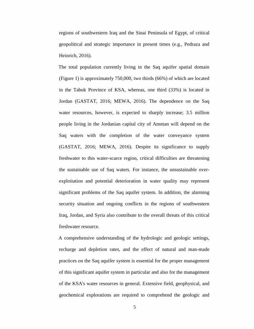
regions of southwestern Iraq and the Sinai Peninsula of Egypt, of critical
geopolitical and strategic importance in present times (e.g., Pedraza and
Heinrich, 2016).
The total population currently living in the Saq aquifer spatial domain
(Figure 1) is approximately 750,000, two thirds (66%) of which are located
in the Tabuk Province of KSA, whereas, one third (33%) is located in
Jordan (GASTAT, 2016; MEWA, 2016). The dependence on the Saq
water resources, however, is expected to sharply increase; 3.5 million
people living in the Jordanian capital city of Amman will depend on the
Saq waters with the completion of the water conveyance system
(GASTAT, 2016; MEWA, 2016). Despite its significance to supply
freshwater to this water-scarce region, critical difficulties are threatening
the sustainable use of Saq waters. For instance, the unsustainable over-
exploitation and potential deterioration in water quality may represent
significant problems of the Saq aquifer system. In addition, the alarming
security situation and ongoing conflicts in the regions of southwestern
Iraq, Jordan, and Syria also contribute to the overall threats of this critical
freshwater resource.
A comprehensive understanding of the hydrologic and geologic settings,
recharge and depletion rates, and the effect of natural and man-made
practices on the Saq aquifer system is essential for the proper management
of this significant aquifer system in particular and also for the management
of the KSA's water resources in general. Extensive field, geophysical, and
geochemical explorations are required to comprehend the geologic and
6
hydrogeological settings of this expansive aquifer system. Additionally,
the development, validation, and calibration of groundwater flow models
are essential for the exploration of the effect of natural and man-made
consequences for this aquifer system. However, the development of such
models, for the most part, requires gathering deep subsurface and field
information, including, but not limited to, temporal water levels, pressure-
driven parameters, and lithological well records. Such data are hard to
acquire for the Saq given its broad spatial distribution, inaccessibility, and
the general absence of local funding to support the required research-
related activities.
The use of recent Earth-observing satellites has greatly facilitated our
ability to observe changes in water resources at large scales (e.g.,
Famiglietti and Rodell, 2013; Famiglietti, 2014). The deployment of the
Gravity Recovery and Climate Experiment (GRACE) mission and the
acquisition of temporal gravity fields provide significant practical
strategies for exploring the temporal mass variations over the Saq and
other expansive aquifer systems across the globe. The joint National Space
and Aeronautics Administration (NASA)/German Aerospace Center
(DLR) GRACE mission was launched on March 2002 to map the Earth's
static and temporal gravity fields (Tapley et al., 2004a, 2004b). GRACE
measures the spatiotemporal variations in the vertically integrated
Terrestrial Water Storage (TWS).
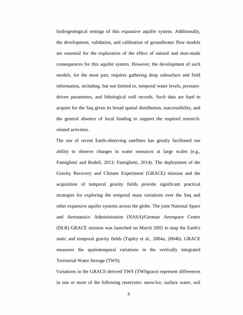
Variations in the GRACE-derived TWS (TWSgrace) represent differences
in one or more of the following reservoirs: snow/ice, surface water, soil
7
moisture, groundwater, and wet biomass (e.g., Wahr et al., 1998). GRACE
data have been extensively used to quantify aquifers recharge and
depletion rates (Ellett et al., 2006; Rodell et al., 2009; Tiwari et al., 2009;
Ahmed et al., 2011, 2014, 2016; Feng et al., 2013; Gonçalvès et al.,
2013; Lenk, 2013; Voss et al., 2013; Joodaki et al., 2014; Wouters et al.,
2014; Castle et al., 2014; Döll et al., 2014; Huang et al., 2015, 2016; Li
and Rodell, 2015; Al-Zyoud et al., 2015; Chinnasamy and Agoramoorthy,
2015; Chinnasamy et al., 2015; Huo et al., 2016; Jiang et al., 2016;
Lakshmi, 2016; Long et al., 2016; Mohamed et al., 2016; Veit and Conrad,
2016; Wada et al., 2016; Yosri et al., 2016; Castellazzi et al., 2016;
Chinnasamy and Sunde, 2016)
In this study, 14 years of monthly (April 2002 to April 2015) GRACE were
utilized and land surface model (LSM) outputs along with the available
geologic, hydrologic, and remote sensing datasets to inspect the spatial and
temporal variations in TWSgrace and GRACE-derived groundwater
storage (GWSgrace) over the Saq aquifer system (Figure 1) to explore the
natural and anthropogenic drivers of these variations. The calculated
GWSgrace estimates were then correlated and validated against field
measurements from 15 groundwater wells distributed across the Saq
aquifer system (Figure 1). Recently, Sultan et al., (2014) used monthly
(January 2003–September 2012) GRACE data to quantify the TWSgrace
depletion over the Saq aquifer. They concluded that excessive groundwater
extraction, not climatic changes, is responsible for the observed TWSgrace
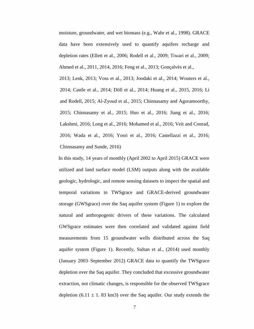
depletion (6.11 ± 1. 83 km3) over the Saq aquifer. Our study extends the
8
investigations of Sultan et al., (2014) by (1) utilizing enhanced state-of-the
art TWSgrace solutions; the global mass concentration solutions
(mascons), (2) utilizing outputs from several LSMs; four versions of the
Global Land Data Assimilation System (GLDAS), to isolate the
GWSgrace, (3) expanding the study area to incorporate the Saq aquifer in
the KSA and Jordan border region, (4) broadening the time interval by
three years, and (5) validating GRACE observations of groundwater
variations with field water level data from regional supply wells.
Study Area
2.1 Geology, Hydrogeology, and Geomorphology
The Arabian Peninsula contains several aquifer systems sitting, in an arc
shape, directly over the Precambrian Arabian Shield (Figure 1). These
aquifer systems could be grouped into (1) Paleozoic (sandstone: Saq, Al-
Wajid, Tabuk; limestone: Khuff) aquifers; (2) Mesozoic (sandstone:
Dhruma, Al-Biyadh and Al-Wasia; limestone/dolomite: Umm-Radmah,
and Al-Dammam) aquifers; and (3) Cenozoic (alluvial deposits) aquifers
(e.g., Al Alawi, J., Abdulrazzak, 1994; Alsharhan and Nairn, 1997).
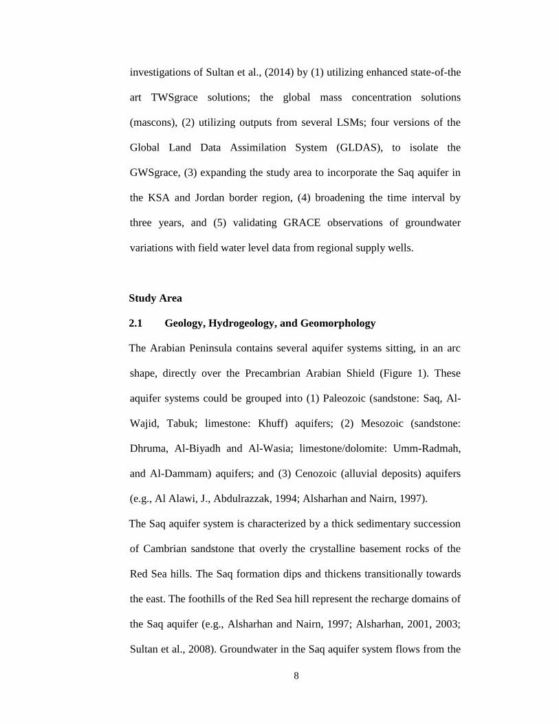
The Saq aquifer system is characterized by a thick sedimentary succession
of Cambrian sandstone that overly the crystalline basement rocks of the
Red Sea hills. The Saq formation dips and thickens transitionally towards
the east. The foothills of the Red Sea hill represent the recharge domains of
the Saq aquifer (e.g., Alsharhan and Nairn, 1997; Alsharhan, 2001, 2003;
Sultan et al., 2008). Groundwater in the Saq aquifer system flows from the
9
west, where the Red Sea Hills are located, towards the east and drains
naturally in and close to the Arabian Gulf. The Saq aquifer is unconfined
in recharge domains in the west and becomes confined towards the
discharge domains in the east (Alsharhan and Nairn, 1997; Alsharhan,
2001, e.g., 2003; Sultan et al., 2008). The water-bearing layer of the Saq
aquifer exhibits a large thickness (400-1200 meters), and high storage
capacity (storage: 258 km3) (BRGM, 2008). The Saq aquifer waters are
believed to have originated, largely, from paleo-precipitation during the
previous wet climatic periods, which recharged the aquifers through
outcrop locations at the foothills of the Red Sea hills. However, recent
studies have also demonstrated that locally, the Saq aquifer is receiving
present- day recharge in regions with moderately high precipitation in
northwestern Red Sea Hills (Beaumont, 1977; Bayumi, 2008; Sultan et al.,
2008, 2011; Wagner, 2011; Abouelmagd et al.,
2012, 2014; Zaidi et al., 2015).
2.2 Shared Water Resources of the Arabian Peninsula
In 1970, the KSA started to use the water of the Saq aquifer for human
consumption; however, the amount of the extracted water increased in
1980 to support wheat production. Wheat is a water- intensive crop, and
this farming effort required a tremendous amount of groundwater
extraction, around 1.0 km3/year (e.g., Ferragina and Greco, 2008). Since
2000, extensive development has been recorded in the region with urban
growth, improved transportation corridors, agricultural expansion, and
associated irrigation projects. These developments have stressed the
10
groundwater resources of the Saq aquifer; in 2000’s the reported
groundwater extraction rates were estimated at 5.7 km3/year (BRGM,
2008).
The Saq is the largest of the shared KSA/Jordan aquifer systems. Unlike
KSA, Jordan has access to renewable surface water via the Jordan River.
Jordan has also planned to dam the Yarmouk, a tributary of the Jordan
River, to form a reservoir with a total capacity of 0.9 km3/year (Ferragina
and Greco, 2008). Jordan uses the Saq aquifer to supply water to the city of
Aqaba and the surrounding areas. Total current Jordanian water
consumption from the Saq aquifer is 0.075 km3/year (Ferragina and Greco,
2008). Jordan, however, plans to increase the exploitation of this aquifer
system, with a project underway to construct a 325-km pipeline from a
well field in the south to the capital city of Amman in the north, which will
supply about 0.1 km3/year to the water- starved region (Ferragina and
Greco, 2008).
3. Data and Methods
A flowchart summarizing the main processing steps applied to GRACE
and other relevant datasets used in this study is shown in Figure 2.
Generally, the soil moisture data were utilized to remove the non-
groundwater storage components from TWSgrace data. Rainfall data used
to explore the climatic controls on the temporal variations in TWSgrace.
Groundwater levels and irrigated areas, among others, were used to
validate GWSgrace results over the Saq aquifersystem.
3.1 GRACE-Derived Total Water Storage (TWSgrace) Data (see
11
Appendix A)
Three sources of GRACE data have been utilized in this study: spherical
harmonics and mascons products of the University of Texas Center for
Space Research (UT-CSR) and mascons solutions from the Jet Propulsion
Laboratory (JPL) in USA. Compared to the spherical harmonic fields, the
mascons solutions provide higher signal-to-noise ratio, higher spatial
resolution, reduced error, and do not require spectral (e.g., de-striping) or
spatial (e.g., smoothing) filtering (Watkins et al., 2015; Save et al., 2016;
Wiese et al., 2016).
The spherical harmonics of UT-CSR GRACE solution (Level 2; Release
05; degree/order: 60) have been utilized in this study. The time-variable
component of the gravity field was obtained by subtracting the temporal
(April 2002 to April 2015) mean from each of the monthly spherical
harmonics values. The systematic and the random errors in the GRACE
datasets were then reduced by describing and Gaussian (200 km) filters,
respectively (Wahr et al., 1998; Swenson and Wahr, 2006). The GRACE
spherical harmonics coefficients were then converted to a TWSgrace grid
of equivalent water thickness (Wahr et al., 1998).
The JPL mascons data (version RL05M_1) provide monthly gravity field
variations for 4,551 equal areas of 3° spherical caps. The Coastline
Resolution Improvement (CRI) filtered data, utilized to determine the land
and ocean fractions of mass inside every land/sea mascon, were used in
this study (Watkins et al., 2015). The UT-CSR mascons solutions (version
v01) approach uses the geodesic grid technique to model the surface of the
12
earth using equal area gridded representation of the earth via 40,962 cells
(40,950 hexagons + 12 pentagons) (Save et al., 2016). The size of each cell
is about equatorial 1°, the number of cells along the equator is 320, and the
average area of each cell is 12,400 km2. The average distance between cell
centers is 120 km. The UT- CSR mascons do not suffer from over-
sampling at the poles like an equiangular grid. No neighboring cells meet
at a single point (Save et al., 2016).
After generating TWSgrace grids from GRACE spherical harmonics and
mascons solutions, trend images were extracted from each of these
solutions by fitting a time series at each grid point using annual and
semiannual sines and cosines, means, and linear trends components
(Figure 3). To examine the temporal variability in TWSgrace over the Saq
aquifer, the TWSgrace grid points lying within the Saq aquifer were
averaged to produce the Saq TWSgrace time series (Figure 4.a). This
rescaling approach, described in Sultan et al. (2014), was used to minimize
the attenuation in the amplitude of the TWSgrace time series due to the
application of GRACE post-processing steps. The uncertainty associated
with the monthly TWSgrace time series among all datasets and TWSgrace
trends were then calculated following the approach advanced by Ahmed et
al., (2016) and Tiwari et al. (2009). In this approach, monthly TWSgrace
time series were fitted using annual, semiannual, and trend terms and
residuals were calculated. These residuals were then smoothed using a 13-
month moving average, a trend was removed, and another set of residuals
were calculated. The standard deviation of the second set of residuals was
13
interpreted as the maximum uncertainty in monthly TWSgrace values. To
calculate the TWSgrace trend errors, Monte Carlo simulations were
performed by fitting trends and seasonal terms for many synthetic monthly
datasets, each with values chosen from a population of Gaussian-
distributed numbers having a standard deviation similar to that of the
second set of residuals. The standard deviation of the extracted synthetic
trends was interpreted as the trend error for TWSgrace. The generated
TWSgrace trend data were then statistically analyzed by using the Student
t-test to identify their significancelevels.
3.2 Land Surface Model-derived TWS Data
Since GRACE has no vertical resolution, the TWS outputs of the GLDAS
model (TWSgldas) were utilized in this studyto enhance the vertical
resolution of TWSgrace data. Compared to other land surface models, the
GLDAS model provides reasonable estimates of soil moisture over an arid
environment of North Africa and Middle East (Ahmed et al., 2016).
GLDAS is a land surface modeling system developed by NASA that
incorporates field and satellite-based observations to drive detailed
advanced simulations of climatic and hydrologic variables (Rodell et al.,
2004). The GLDAS model simulates TWSgldas (summation of soil
moisture, snow, and canopy storages) through four model versions: VIC,
Noah, MOSAIC, and CLM (Koster and Suarez, 1996; Liang et al., 1996;
Koren et al., 1999; Dai et al., 2003). The four GLDAS versions (e.g., VIC,
Noah, Mosaic, and CLM), were used in this study after subtraction of the
temporal (April 2002 to April 2015) mean from each version. Given the
14
fact that the Saq aquifer is located in a hyper-arid region with minimal
vegetation and no surface water reservoirs, the GLDAS-derived snow and
canopy storages were neglected. The mean soil moisture estimates of the
four TWSgldas simulations (e.g., VIC, Noah, Mosaic, and CLM), were
calculated and then subtracted from TWSgrace estimates to quantify the
GWSgrace variability over the Saq aquifer system. Errors in GLDAS-
derived soil moisture (SMgldas) estimates were calculated as the standard
deviations of the soil moisture values computed from the four GLDAS
simulations. The final GWSgrace uncertainties were calculated by
summing, in quadrature, the contributions from TWSgrace errors to
SMgldas errors. The spatial variability in GWSgrace trends are shown in
Figure 5.
3.3 Rainfall Data
Precipitation data were utilized to explore the climatic controls on the
temporal variation in TWSgrace observed over the Saq aquifer system.
The Climate Prediction Center (CPC) Merged Analysis of Precipitation
(CMAP) dataset was utilized in this study. CMAP data provide global
(88.75°N to 88.75°S) merged precipitation estimates from a variety of
satellite and ground-based sources from January 1979 to June 2016 with
spatial and temporal resolutions of 2.5° and one month, respectively (Xie
and Arkin, 1997). The temporal difference in average annual precipitation
(AAP), calculated from CMAP data, for the periods 2002-2015 and 1979-
2001 was calculated and mapped over the entire Arabian Peninsula (Figure
6). AAP data were used to explore the climatic control on TWSgrace given
15
the fact that a rainfall value is already a rate, and so it corresponds to a
trend (i.e., a mass/time) signal in the TWSgrace; a trend in rainfall
corresponds to an increase in mass rate, and so to a quadratic function of
time in the mass.
3.4 Field Data
Water level data of 15 monitoring wells distributed over the entire Saq
aquifer system in the KSA (Figure 1) and maintained by Ministry of
Environment, Water, and Agriculture in theKSA, over the period from
2002 through 2016, were used in this study. Water level data were used to
validate the GWSgrace variability of the Saq aquifer system. The selection
of these wells is justified by their particular characteristics and availability
of data during the study period. Only the monitoring wells that show
nearly continuous monthly water level records were selected.
These wells are located in two KSA provinces: The Tabuk Province (13
wells: 1T052S, 1T058S, 1H060S, 1T063S, 1T072S, 1T074S, 1T075S,
1T097S, 1T098S, 1T099, 1T107S, 1T114S, and 1T3053S; Figure 1) and
the Al Jawf Province (2 wells, SK-624-T and SK-625-P; Figure 1). The
Tabuk and Al Jawf areas represent the most irrigated provinces in KSA. In
these provinces, modern irrigation (e.g., localized and sprinkler) represent
about 89% of the irrigation activities, while the remaining 11% is under
flood irrigation (GASTAT, 2016). Following the approach advanced by
previous similar studies (e.g., Castle et al., 2014), given the lack of specific
yield information from examined wells, the water level time series was
normalized for each monitoring well by its standard deviation with the
16
following method: (1) the mean and the standard deviation for each well
time series were calculated; (2) the mean was subtracted and the mean-
removed water levels were divided by standard deviation to get the
normalized water level value (Jutla et al., 2006) (Figure 7).
3.5 Normalized Difference Vegetation Index (NDVI)
The spatial distribution of irrigated areas (Figure 8a) extracted from the
global map of irrigation areas (Siebert et al., 2017), as well as the spatial
distribution in the NDVI trends (Figure 8b) and the NDVI time series
(Figure 9) were used to validate GWSgrace results over the Saq aquifer.
The Moderate-resolution Imaging Spectroradiometer (MODIS)–derived
NDVI products were used in this study. NDVI data were generated from
global monthly level-3 MODIS Terra (MOD13C2; spatial resolution:
0.05º) (Justice et al. 1998; 2002).
4. RESULTS AND DISCUSSION
4.1 GRACE-derived TWS (TWSgrace) Trend
The TWSgrace secular trends over the Arabian Peninsula are displayed in
Figure 3.The areas in the southern parts of the Arabian Peninsula exhibit
minimal variations in TWSgrace (secular trend ~ 0 mm/year), whereas
areas in the northern parts of the Arabian Peninsula coincide with the
spatial distribution of the Saq aquifer in the KSA and Jordan, exhibiting
strong negative TWSgrace trends (Figure 3). The TWSgrace anomalies
decrease with time over the negative trend anomalies (shades of blue in
Figure 3). The spatial distributions of negative TWSgrace trend anomalies
vary slightly with the source of GRACE data. In the case of the UT-CSR
17
mascons solutions, the negative trend areas are closely centered over the
Saq aquifer, whereas these areas extend beyond the spatial distribution of
the Saq aquifer in the case of the JPL mascons and UT-CSR spherical
harmonic solutions. This is probably related to the way that the TWSgrace
products have been generated. Among others, JPL mascons were generated
from 3° spherical caps, UT-CSR mascons were generated from 1°
hexagons, and UT-CSR spherical harmonics were smoothed using 200 km
Gaussian filter (spatial resolution ~ 125,000 km2).
Temporal variations in the TWSgrace time series generated over the Saq
aquifer system shows a depletion in the TWSgrace estimates extracted
from UT-CSR mascons, JPL mascons, and UT- CSR spherical harmonic
solutions (Figure 4a). Depletion rates of -8.96 ± 0.27 mm/year (-4.79 ±
0.14 km3/year), -9.65 ± 0.26 mm/year (-5.16± 0.13 km3/year), and -8.60 ±
0.31 mm/year (-4.60 ± 0.16 km3/year) were observed in TWSgrace
estimates of UT-CSR and JPL mascons, and UT- CSR spherical harmonic
solutions, respectively. The average depletion rate over the entire Saq
system, as calculated from the mean of the three solutions (black line;
Figure 4.a), is estimated at -9.05 ± 0.25 mm/year (-4.84 ± 0.13 km3/year).
All of the reported TWSgrace trends are significant at the < 0.001%
significance level. Errors in the average of the three solutions (black line;
Figure 4.a) were calculated by adding, in quadrature, errors associated with
each solution.
The question of whether the observed TWSgrace negative trend anomalies
over the Saq aquifer system (Figure 3) are caused by natural factors (such
18
as global warming and associated changes in the amounts, patterns, and
frequencies of precipitation) and/or by anthropogenic factors (such as
increased domestic groundwater withdrawal for urbanization and irrigation
activities) are addressed by examining climatic data over the Arabian
Peninsula. Recent studies (e.g., Bucchignani et al., 2015) have shown that,
in arid and semi-arid areas, precipitation represents one of the primary
climatic forcing parameters, whereas other climatic parameters such as
specific humidity, wind speed, surface pressure, and solar radiation play a
secondary role. Accordingly, the spatial and temporal variability in rainfall
rates over the Arabian Peninsula were examined.
To check the mutual effects of variations in rainfall on the TWSgrace, the
changes of the Annual Average Precipitation (AAP) over the last decade
(2002-2015) were examined relative to that of the previous two decades
(1979-2001) (Figure 6a). Areas that exhibit a decline in rainfall over 2002-
2015 are shown in the shades of blue, whereas areas experiencing an
increase in rainfall over 1979-2001 are shown in the shades of red. If the
TWSgrace negative trend over the Saq aquifer is partially related to
decline in rainfall, one would expect to see significantly reduced AAP
rates throughout the examined time period (2002-2015) compared to the
recorded precipitation for the preceding period (1979-2001) given the fact
that the ground and soil are drying out. Figure 6a shows that the Saq
aquifer system experienced a decline in rainfall over the past decade. The
reduction in rainfall over the Saq aquifer system is also evident from the
analysis of rainfall time series extracted from CMAP data) Figure 6b (.
19
Figures 6a and b indicate that the decline in rainfall rates is apparent in a
comparison of AAP for the investigated period to that of the previous 23
years (AAP for 1979- 2001: 104 mm; AAP for 2002-2015: 60 mm; Figs.
6a, b). Declines are higher in the southern and the central parts of the Saq
aquifer; this could be related to changes in wind regime and/or
atmospheric circulations prevailing these areas (e.g., Alsharhan 2001).
Figure 6a is correlated, to a more significant extent, with the TWSgrace
trends extracted from UT-CSR mascons data (Figure 3a) and, to lesser
extent, with TWSgrace trends extracted from UT-CSR spherical harmonics
(Figure 3c). This might indicate that the observed TWSgrace depletions,
seen in Figures 3a and 3c, are strictly related to climate change. However,
Figure 6a doesn’t seem to match well the TWSgrace trends extracted from
JPL mascons data (Figure 3b). This might be consistent with the
anthropogenic factors (e.g., groundwater extraction) as being a cause of
TWSgrace depletion.
4.2 GRACE-derived GWS (GWSgrace) Trend
The observed TWSgrace depletions over the Saq aquifer are related to
variations in both soil moisture storage and GWS since there are no surface
water inputs. To quantify the GWSgrace variations over the Saq aquifer
system (Figure 5), the SMgldas estimates (average of VIC, Noah, Mosaic,
and CLM versions) are subtracted from the TWSgrace (averaged from UT-
CSR mascons, JPL mascons, and UT-CSR spherical harmonic solutions).
The spatial distribution in GWSgrace (Figure 5) reveals that the entire
Arabian Peninsula is witnessing GWSgrace depletion, except the
20
southwestern parts of Yemen (GWSgrace trend: > 1 mm/yr). Areas in the
northern parts of the Arabian Peninsula coincide with the spatial
distribution of the Saq aquifer in the KSA and Jordan, exhibiting strong
negative GWSgrace trends of up to -8.85 mm/yr.
Errors in GWSgrace were calculated by adding, in quadrature, errors
associated with GWSgrace and SMgldas estimates. Figure 4b shows a
groundwater depletion rate of -6.52 ± 0.29 mm/year, equivalent to -3.49 ±
0.15 km3/year over the Saq aquifer system during the investigated (April
2002 to April 2015) period. The reported GWSgrace trend is significant at
< 0.001% significance level. The GWSgrace depletion rate indicates that
more than 70% of the TWSgrace variability over the Saq aquifer system is
controlled by GWS variabilities.
To validate the GWSgrace variability, the normalized GWSgrace were
compared with groundwater level observations of 15 monitoring wells
(Figure 7) distributed throughout the Saq aquifer (locations shown in
Figure 1). To the best of our knowledge, this is the first-time field data
from water supply wells, within the vulnerable Saq aquifer region, has
been used to directly validate TWSgrace and/or GWSgrace estimates.
Comparisons indicated that the GWSgrace estimates generally capture the
observed groundwater level depletion shown by the analysis of water level
data (Figure 5). The observed GWSgrace depletions over the Saq aquifer
are attributed to extensive groundwater extraction activities mainly from
the Saq aquifer system. These activities were intended to develop
agricultural communities in northern and northwestern parts of the Arabian
21
Peninsula.
Our interpretation is supported by the reported groundwater extraction
rates as well as the observed variations in the areas and the spatial
distribution of the irrigated regions and irrigation wells (Figure 8a). Figure
8a shows that areas that are witnessing GWSgrace depletion (Figure 5)
coincide with a broad part of irrigation and intensive groundwater
extraction (Figure 8a), suggesting that the negative GWSgrace trend is a
result of that extraction. Moreover, in the 1960s, groundwater extraction
from the Saq aquifer in the KSA was as small as 0.1 km3/year and
increased to 2.0 km3 and in the 1980's and to 8.7 km3 in the 2000's
(BRGM, 2008). In the KSA, extraction from the Saq aquifer itself
represents 65% to 70% of the reported extraction rates (BRGM, 2008).
The reported groundwater extraction rates from the Saq aquifer itself were
estimated at 1.4 km3 in the 1980's and 5.7 km3 in the 2000's.
The spatial variations in the NDVI trends (Figure 8b), as well as the
temporal changes in the NDVI (Figure 9), extracted from Landsat TM
data, over the entire Saq aquifer system, supports the fact that the
GWSgrace depletions are related to extensive groundwater extraction
activities for agricultural purposes. Figure 8b reveals positive NDVI trends
correlated with the heavily irrigated areas (Figure 8a) that are witnessing
GWSgrace depletions (Figure 5). Figure 9 shows a moderate decrease in
the NDVI values until the beginning of 2007, and then a bright switch to a
positive trend, which coincides strongly, in trends, with the increase in
TWSgrace and GWSgrace (Figure 4) depletion rates.
22
4.3. Factor driving TWSgrace and GWSgrace depletions
Freshwater resources in the Saq aquifer system are extremely vulnerable to
both climatic and anthropogenic factors. The variations in total and
groundwater storage (TWSgrace and GWSgrace) data over the past
fourteen years (April 2002-April 2015) indicates the following:
(1) The Saq aquifer system is witnessing rapid TWSgrace and GWSgrace
depletion rates of -9.05 ± 0.25 mm/year (-4.84 ± 0.13 km3/year) and -6.52
± 0.29 mm/year (-3.49 ± 0.15 km3/year), respectively, related to both
climatic and anthropogenic factors; (2) the observed TWSgrace depletion
rate is partially related to a decline in rainfall as is evident from a
comparison of AAP for the investigated period to the previous 23 years
(AAP for 1979-2001: 104 mm; AAP for 2002-2015: 60 mm); (3) the
observed TWSgrace depletion rate is largely attributed to groundwater
extraction activities for irrigation; and (4) the observed GWSgrace
depletion is correlated with the observed water level depletion rates in
water supply wells within the aquifer region.
Our findings are in agreement with other researchers’ results that indicate
the Saq aquifer is witnessing TWSgrace depletion. However, the rates of,
and the factors controlling, the observed TWSgrace and GWSgrace
depletions are slightly different. For example, Sultan et al., (2014)
indicated that only excessive groundwater extraction, not climatic changes,
is responsible for the observed TWSgrace depletion (6.11 ± 1. 83 km3/yr)
over the Saq aquifer during the period from January 2003 to September
2012. Similarly, Joodaki et al., (2014) have concluded that during the
23
period from February 2003 to December 2012, the northern KSA region,
has witnessed a decline in TWSgrace that is mainly due to a decline in
GWSgrace (6.0 ± 3.0 km3/yr). The observed differences between the
previous and our findings could be, among others, attributed to the changes
in the investigated time, investigated area, and the data source.
It is worth mentioning that, the mascons solutions, used in our study,
provide higher signal to noise ratio, higher spatial resolution, reduced
error, and do not require spectral and spatial filtering or any experimental
scaling techniques. As a result, our results report far better accuracy and
much smaller error margins (an order of magnitude lower) in the TWS and
GWS estimates. Our GWSgrace depletion rates are highly correlated with
the observed decline in water level measured in water supply wells within
the investigated aquifer system.
The rapid declines in GWSgrace in this extremely arid, strategic, and
geopolitically significant region needs to be carefully monitored and
managed with competing uses within KSA and plans to use the Saq aquifer
to supply freshwater to the Jordanian capital city of Amman. Our results
indicate that the implications of unsustainable groundwater based irrigation
and extraction practices are clear for these fossil aquifers, also warranting
future investigation on the impacts on water quality changes in the
valuable sources. Our study also demonstrates that global monthlyGRACE
24
solutions can provide a practical, informative, and cost-effective method
for monitoring aquifer systems in water-stressed regions across the globe.
5. Conclusion
Water is a valuable resource in the Arabian Peninsula’s current hyper-arid
conditions. In KSA, for example, there are no surface water rivers or
reservoirs. To sustain its growing population, KSA is currently utilizing
more of its groundwater resources and is planning to increase the
groundwater extraction rates in the near future. The lack of an
understanding of the available groundwater resources and the
spatiotemporal depletion rates and locations along with the factors
controlling these depletions are posing enormous challenges to the general
population of KSA. This study included an integrated, cost-effective
approach that combines the state-of-art GRACE data along with other
relevant land surface models, remote sensing, geological, and hydrological
data and GIS techniques to examine the spatiotemporal variations in the
groundwater resources of the Saq aquifer system and to explore the natural
and anthropogenic drivers of these variations. Results of this study will
contribute to the effective and efficient utilization of the Saq aquifer water
resources and will be used to promote the sustainable development of the
Arabian Peninsula’s natural resources in general. The study findings are
being be shared with decision-makers in relevant governmental agencies to
develop sustainable management scenarios for the Saq aquifer water
resources.
25
6. Acknowledgments
This research was supported, in part, by NASA Health and Air Quality
grant (NNX15AF71G). The authors would like to thank the Ministry of
Water and Electricity of the Kingdom of Saudi Arabia, Water Information
Department for providing the field data to support this research.
26
7. References:
1. Abouelmagd A, Sultan M, Milewski A, Kehew AE, Sturchio NC,
Soliman F, Krishnamurthy R V., Cutrim E. 2012. Toward a better
understanding of palaeoclimatic regimes that recharged the fossil
aquifers in North Africa: Inferences from stable isotope and remote
sensing data. Palaeogeography, Palaeoclimatology, Palaeoecology
329–330: 137–149 DOI: 10.1016/j.palaeo.2012.02.024.
2. Abouelmagd A, Sultan M, Sturchio NC, Soliman F, Rashed M,
Ahmed M, Kehew AE, Milewski A, Chouinard K. 2014.
Paleoclimate record in the Nubian Sandstone Aquifer, Sinai
Peninsula, Egypt. Quaternary Research (United States) 81 (1):
158–167 DOI: 10.1016/j.yqres.2013.10.017
3. Ahmed M, Sultan M, Wahr J, Yan E. 2014. The use of GRACE
data to monitor natural and anthropogenic induced variations in
water availability across Africa. Earth-Science Reviews 136:
289–300 DOI: 10.1016/j.earscirev.2014.05.009
4. Ahmed M, Sultan M, Wahr J, Yan E, Milewski A, Sauck W,
Becker R, Welton B. 2011.Integration of GRACE ( Gravity
Recovery and Climate Experiment ) data with traditional data sets for a
better understanding of the time-dependent water partitioning in
African watersheds. (5): 479–482 DOI: 10.1130/G31812.1
5. Ahmed M, Sultan M, Yan E, Wahr J. 2016. Assessing and
27
Improving Land Surface Model Outputs over Africa using
GRACE, Field, and Remote Sensing Data. Surveysin Geophysics
37 (3): 529–556 DOI: 10.1007/s10712-016-9360-8
6. Al-Zyoud S, Rühaak W, Forootan E, Sass I. 2015. Over
Exploitation of Groundwater in the Centre of Amman Zarqa
Basin—Jordan: Evaluation of Well Data and GRACE Satellite
Observations. Resources 4 (4): 819–830 DOI:
10.3390/resources4040819
7. Al Alawi, J., Abdulrazzak M. 1994. Water in the Arabian
Penninsula: problems and perspectives. In Water in the Arab
World; Perspectives and Prognoses., Rogers, P., Lydon P
(ed.).Harvard University Press; 171–202.
8. Alsharhan AS. 2001. Hydrogeology of an arid region : the
Arabian Gulf and adjoining areas. Elsevier.
9. Alsharhan AS. 2003. Petroleum geology and potential
hydrocarbon plays in the Gulf of Suez rift basin, Egypt. AAPG
Bulletin 87 (1): 143–180 DOI: 10.1306/062002870143
10. Alsharhan AS, Nairn AEM. 1997. Sedimentary basins and
petroleum geology of the Middle East. Elsevier.
11. Bayumi T. 2008. Quantitative Groundwater Resources
Evaluation in the Lower Partof Yalamlam Basin, Makkah Al
Mukarramah, Western Saudi Arabia. Journal of King Abdulaziz
University-Earth Sciences 19: 35–56 DOI: 10.4197/Ear.19-1.3
28
12. Beaumont P. 1977. Water and Development in Saudi Arabia. The
Geographical Journal 143 (1): 42 DOI: 10.2307/1796674
13. BRGM. 2008. Bureau de Recherches Géologiques et Minières:
Investigations for updating the groundwater mathematical
model(s) of the Saq and overlyingaquifers (BRGM, ed.).
Ministry of Water and Electricity: Kingdom of Saudi Arabia.
14. Bucchignani E, Cattaneo L, Panitz H-J, Mercogliano P. 2015.
Sensitivity analysiswith the regional climate model COSMO-
CLM over the CORDEX-MENA domain. Meteorology and
Atmospheric Physics DOI: 10.1007/s00703-015-0403-3
15. Castellazzi P, Martel R, Galloway DL, Longuevergne L, Rivera
A. 2016. Assessing Groundwater Depletion and Dynamics Using
GRACE and InSAR: Potential and Limitations. Groundwater 54
(6): 768–780 DOI: 10.1111/gwat.12453
16. Castle S, Thomas B, Reager J, Rodell M, Swenson S, Famiglietti
J. 2014. Groundwater depletion during drought threatens future
water security of the Colorado River Basin. Geophysical
Research Letters 10: 5904–5911 DOI:
10.1002/2014GL061055.Received
17. Chinnasamy P, Agoramoorthy G. 2015. Groundwater Storage
and Depletion Trendsin Tamil Nadu State, India. Water
Resources Management 29 (7): 2139–2152 DOI:
10.1007/s11269-015-0932-z
29
18. Chinnasamy P, Sunde MG. 2016. Improving spatiotemporal
groundwater estimates after natural disasters using remotely
sensed data – a case study of the Indian Ocean Tsunami. Earth
Science Informatics 9 (1): 101–111 DOI: 10.1007/s12145-015-
0238-y
19. Chinnasamy P, Maheshwari B, Prathapar S. 2015. Understanding
groundwater storage changes and recharge in Rajasthan, India
through remote sensing. Water (Switzerland) 7 (10): 5547–5565
DOI: 10.3390/w7105547
20. Dai Y, Zeng X, Dickinson RE, Baker I, Bonan GB, Bosilovich
MG, Denning a. S, Dirmeyer P a., Houser PR, Niu G, et al. 2003.
The common land model. Bulletin of the American
Meteorological Society 84 (8): 1013–1023 DOI: 10.1175/BAMS-
84-8-1013
21. Döll P, Müller Schmied H, Schuh C, Portmann FT, Eicker A.
2014. Global-scale assessment of groundwater depletion and
related groundwater abstractions: Combining hydrological
modeling with information from well observations and GRACE
satellites. Water Resources Research 50 (7): 5698–5720 DOI:
10.1002/2014WR015595
22. Ellett KM, Walker JP, Western AW, Rodell M. 2006. A
framework for assessing the potential of remote-sensed gravity to
provide new insight on the hydrology of the Murray-Darling
30
Basin. Australasian Journal of Water Resources 10: 125–138
23. Famiglietti JS. 2014. The global groundwater crisis. Nature
Climate Change 4 (11): 945– 948 DOI: 10.1038/nclimate2425
24. Famiglietti JS, Rodell M. 2013. Water in the balance. Science
340: 1300–1301 DOI: 10.1126/science.1236460
25. Feng W, Zhong M, Lemoine J-M, Biancale R, Hsu H-T, Xia J.
2013. Evaluation of groundwater depletion in North China using
the Gravity Recovery and Climate Experiment (GRACE) data
and ground-based measurements. Water ResourcesResearch 49
(4): 2110–2118 DOI: 10.1002/wrcr.20192
26. Ferragina E, Greco F. 2008. The Disi project: an internal/external
analysis. Water International 33 (4): 451–463 DOI:
10.1080/02508060802504412
27. GASTAT. 2016. General Authority for Statistics Available at
http://www.stats.gov.sa/en [Accessed 24 December 2016]
28. Gonçalvès J, Petersen J, Deschamps P, Hamelin B, Baba-Sy O.
2013. Quantifying the modern recharge of the ‘fossil’ Sahara
aquifers. Geophysical Research Letters 40 (11): 2673–2678 DOI:
10.1002/grl.50478
29. Huang J, Pavlic G, Rivera A, Palombi D, Smerdon B. 2016.
Mapping groundwater storage variations with GRACE: a case
study in Alberta, Canada. Hydrogeology Journal: 1663–1680
DOI: 10.1007/s10040-016-1412-0
31
30. Huang Z, Pan Y, Gong H, Yeh PJF, Li X, Zhou D, Zhao W.
2015. Subregional-scale groundwater depletion detected by
GRACE for both shallow and deep aquifers in North China Plain.
Geophysical Research Letters 42 (6): 1791–1799 DOI:
10.1002/2014GL062498
31. Huo A, Peng J, Chen X, Deng L, Wang G, Cheng Y. 2016.
Groundwater storage and depletion trends in the Loess areas of
China. Environmental Earth Sciences 75 (16): 1–11 DOI:
10.1007/s12665-016-5951-4
32. Jiang Q, Ferreira VG, Chen J. 2016. Monitoring groundwater
changes in the Yangtze River basin using satellite and model
data. Arabian Journal of Geosciences 9 (7) DOI:
10.1007/s12517-016-2522-7
33. Joodaki G, Wahr J, Swenson S. 2014. Estimating the human
contribution to groundwater depletion in the Middle East, from
grace data, land surface models, and well observations
Gholamreza. Water Resources Research 50: 1–14 DOI:
10.1002/2013WR014633.Received
34. Justice C., Townshend JR., Vermote E., Masuoka E, Wolfe R.,
Saleous N, Roy D., Morisette J. 2002. An overview of MODIS
Land data processing and product status. Remote Sensing of
Environment 83 (1): 3–15 DOI:10.1016/S0034-4257(02)00084-6
35. Justice CO, Vermote E, Townshend JRG, Defries R, Roy DP,
32
Hall DK, Salomonson VV, Privette JL, Riggs G, Strahler A, et al.
1998. The Moderate Resolution Imaging Spectroradiometer
(MODIS): land remote sensing for global change research. IEEE
Transactions on Geoscience and Remote Sensing 36 (4): 1228–
1249 DOI: 10.1109/36.701075
36. Kinzelbach W, Aeschbach W, Alberich C, Baba GI, Beyerle U,
Brunner P, Chiang Wen- Hsing, Rueedi J, Zoellmann K. 2002. A
survey of methods for groundwater recharge in arid and semi-
arid regions | Protos. Nairobi UNEP - United Nations
Environment Programme KE: Nairobi. Available at:
http://www.protos.ngo/en/survey-methods- groundwater-
recharge-arid-and-semi-arid-regions [Accessed 24 December
2016]
37. Koren V, Schaake J, Mitchell K, Duan Q, Chen F, Baker JM.
1999. A parameterization of snowpack and frozen ground
intended for NCEP weather and climate models. Journal of
Geophysical Research 104: 19569–19585 DOI:
10.1029/1999JD900232.
38. Koster RD, Suarez MJ. 1996. Energy and Water Balance
Calculations in the Mosaic LSM. NASA Technical Memorandum
104606, 76
39. Lakshmi V. 2016. Beyond GRACE: Using Satellite Data for
Groundwater Investigations. Groundwater 54 (5): 615–618 DOI:
33
10.1111/gwat.12444
40. Lenk O. 2013. Satellite-based estimates of terrestrial water
storage variations in Turkey. Journal of Geodynamics 67 (March
2003): 106–110 DOI: 10.1016/j.jog.2012.04.010
41. Li B, Rodell M. 2015. Evaluation of a model-based groundwater
drought indicator in the conterminous U.S. Journal of Hydrology
526: 78–88 DOI: 10.1016/j.jhydrol.2014.09.027
42. Liang X, Lettenmaier DP, Wood EF. 1996. One-dimensional
statistical dynamic representation of subgrid spatial variability of
precipitation in the two-layer variable infiltration capacity model.
Journal of Geophysical Research 101 (D16): 21403 DOI:
10.1029/96JD01448
43. Long D, Chen X, Scanlon BR, Wada Y, Hong Y, Singh VP,
Chen Y, Wang C, Han Z, Yang W. 2016. Have GRACE satellites
overestimated groundwater depletion in the Northwest India
Aquifer? Scientific reports 6 (April): 24398 DOI:
10.1038/srep24398
44. MEWA. 2016. Ministry of Environment, Water, and Agriculture
Available at
http://www.mowe.gov.sa/enindex.aspx?AspxAutoDetectCookieS
upport=1 [Accessed 25 December 2016]
45. Mohamed A, Sultan M, Ahmed M, Yan E, Ahmed E. 2016.
Aquifer recharge, depletion, and connectivity: Inferences from
34
GRACE, land surface models, geochemical, and geophysical
data. GSA Bullitin: 1–13 DOI: 10.1130/B31460.1
46. Pedraza L, Heinrich M. 2016. Water Scarcity: Cooperation or
Conflict in the MiddleEast and North Africa? Foreign Policy
Journal Available at
http://www.foreignpolicyjournal.com/2016/09/02/water-scarcity-
cooperation-or-conflict- in-the-middle-east-and-north-africa/
[Accessed 24 December 2016]
47. Richey AS, Thomas BF, Lo M-H, Reager JT, Famiglietti JS,
Voss K, Swenson S, Rodell
48. M. 2015. Quantifying renewable groundwater stress with
GRACE. Water Resources Research 51 (7): 5217–5238 DOI:
10.1002/2015WR017349
49. Rodell M, Houser PR, Jambor U, Gottschalck J, Mitchell K,
Meng C-J, Arsenault K, Cosgrove B, Radakovich J, Bosilovich
M, et al. 2004. The global land data assimilation system. Bulletin
of the American Meteorological Society 85 (3): 381–394 DOI:
10.1175/BAMS-85-3-381
50. Rodell M, Velicogna I, Famiglietti JS. 2009. Satellite-based
estimates of groundwater depletion in India. Nature 460 (7258):
999–1002 DOI: 10.1038/nature08238
51. Save H, Bettadpur S, Tapley B. 2016. High-resolution CSR
GRACE RL05 mascons. Journal of Geophysical Research
35
52. Scanlon BR, Healy RW, Cook PG. 2002. Choosing appropriate
techniques for quantifying groundwater recharge. Hydrogeology
Journal 10 (1): 18–39 DOI: 10.1007/s10040-001-0176-2
53. Sultan M, Ahmed M, Wahr J, Yan E, Emil MK. 2014.
Monitoring Aquifer Depletion from Space : Case Studies from
the Saharan and Arabian Aquifers. In Remote Sensing of the
Terrestrial Water Cycle, Lakshmi, V. (ed.).AGU Geophysical
Monograph # 206; 349–366.
54. Sultan M, Metwally S, Milewski a., Becker D, Ahmed M, Sauck
W, Soliman F, Sturchio N, Yan E, Rashed M, et al. 2011.
Modern recharge to fossil aquifers: Geochemical, geophysical,
and modeling constraints. Journal of Hydrology 403 (1–2): 14–
24 DOI: 10.1016/j.jhydrol.2011.03.036
55. Sultan M, Sturchio N, Al Sefry S, Milewski a., Becker R, Nasr I,
Sagintayev Z. 2008. Geochemical, isotopic, and remote sensing
constraints on the origin and evolution of the Rub Al Khali
aquifer system, Arabian Peninsula. Journal of Hydrology 356 (1–
2): 70–83 DOI: 10.1016/j.jhydrol.2008.04.001
56. Swenson S, Wahr J. 2006. Post-processing removal of correlated
errors in GRACE data. Geophysical Research Letters 33 (8):
L08402 DOI: 10.1029/2005GL025285
57. Tapley BD, Bettadpur S, Ries JC, Thompson PF, Watkins MM.
2004a. GRACE measurements of mass variability in the Earth
36
system. Science (New York, N.Y.) 305 (5683): 503–5 DOI:
10.1126/science.1099192
58. Tapley BD, Bettadpur S, Watkins M, Reigber C. 2004b. The
gravity recovery and climate experiment: Mission overview and
early results. Geophysical Research Letters 31 (9): 1– 4 DOI:
10.1029/2004GL019920
59. Tiwari VM, Wahr J, Swenson S. 2009. Dwindling groundwater
resources in northern India, from satellite gravity observations.
Geophysical Research Letters 36 (18):L18401 DOI:
10.1029/2009GL039401 Veit E, Conrad CP. 2016. The impact of
groundwater depletion on spatial variations in sea level change
during the past century. Geophysical Research Letters 43 (7):
3351– 3359 DOI: 10.1002/2016GL068118
60. Voss K a, Famiglietti JS, Lo M, Linage C, Rodell M, Swenson
SC. 2013. Groundwater depletion in the Middle East from
GRACE with implications for transboundary water management
in the Tigris-Euphrates-Western Iran region. Water resources
research 49 (2): 904–914 DOI: 10.1002/wrcr.20078
61. Wada Y, Lo M-H, Yeh PJ-F, Reager JT, Famiglietti JS, Wu R-J,
Tseng Y-H. 2016. Fate of water pumped from underground and
contributions to sea-level rise. Nature Climate Change IN PRESS
(May): 8–13 DOI: 10.1038/nclimate3001
62. Wagner W. 2011. Groundwater in the Arab Middle East. DOI:
37
10.1007/978-3-642- 19351-4
63. Wahr J, Molenaar M, Bryan F. 1998. Time variability of the
Earth’s gravity field: Hydrological and oceanic effects and their
possible detection using GRACE. Journal of Geophysical
Research 103 (B12): 30205–30229 DOI: 10.1029/98JB02844
64. Watkins MM, Wiese DN, Yuan D, Boening C, Landerer FW.
2015. Improved methods for observing Earth’s time-variable
mass distribution with GRACE using spherical cap mascons.
Journal of Geophysical Research : Solid Earth 120: 2648–2671
DOI: 10.1002/2014JB011547.Received
65. Wiese DN, Landerer FW, Watkins MM. 2016. Quantifying and
reducing leakage errors in the JPL RL05M GRACE mascon
solution. Water Resources Research 52 (9): 7490– 7502 DOI:
10.1002/2016WR019344
66. Wouters B, Bonin J a, Chambers DP, Riva REM, Sasgen I, Wahr
J. 2014. GRACE, time- varying gravity, Earth system dynamics
and climate change. Reports on Progress in Physics 116801 DOI:
10.1088/0034-4885/77/11/116801
67. Xie P, Arkin P a. 1997. Global Precipitation: A 17-Year Monthly
Analysis Based on Gauge Observations, Satellite Estimates, and
Numerical Model Outputs. Bulletin of the American
Meteorological Society 78 (11): 2539–2558 DOI: 10.1175/1520-
0477(1997)078<2539:GPAYMA>2.0.CO;2
38
68. Yosri AM, Abd-Elmegeed MA, Hassan AE. 2016. Assessing
groundwater storage changes in the Nubian aquifer using
GRACE data. Arabian Journal of Geosciences 9 (10): 1–9 DOI:
10.1007/s12517-016-2593-5
69. Zaidi FK, Nazzal Y, Ahmed I, Naeem M, Jafri MK. 2015.
Identification of potential artificial groundwater recharge zones
in Northwestern Saudi Arabia using GIS and Boolean logic.
Journal of African Earth Sciences 111: 156–169 DOI:
10.1016/j.jafrearsci.2015.07.008
39
Figure Legends:
Figure 1: (a) Location map showing the spatial distribution of major aquifer
outcrops in the KSA and Jordan, spatial domain of the Saq aquifer system
(red dashed polygon), and distribution of groundwater wells (black circles)
within the KSA's borders
Figure 2: A flowchart showing the main processing steps applied to
Gravity Recovery and Climate Experiment (GRACE) and other relevant
datasets used in this study. JPL = Jet Propulsion Laboratory; NDVI =
normalized difference vegetation index; TWS = terrestrial water storage;
UT‐CSR = University of Texas Center for Space Research
Figure 3: Secular trend images of TWSgrace estimates generated from (a)
UT-CSR mascons, (b) JPL mascons, and (c) UT-CSR spherical harmonics
over the Arabian Peninsula from April 2002 to April 2015.
Figure 4: (A) Temporal variation in TWSgrace estimates, along with the
associated uncertainties, extracted from the UT-CSR mascons (blue line),
JPL mascons (green line), UT-CSR spherical harmonics (red line), and
average (black line) solutions over the Saq aquifer system. (b) Temporal
variation in the GWSgrace estimates over the Saq aquifer system. All of the
reported TWSgrace and GWSgrace trends are significant at > 0.001%
significance level.
Figure 5: Secular trend in GWSgrace estimates generated over the Arabian
Peninsula from April 2002 to April 2015.
40
Figure 6: Difference in Average Annual Precipitation (AAP, mm)
between 2002-2015 period and 1979-2001 period over the Arabian
Peninsula.
Figure 7: Validation of the Gravity Recovery and Climate
Experiment‐derived groundwater storage (GWSgrace) storage
anomalies (black solid thick line) against the available monthly well
observations (individual well: colored circles; average: blue thick line)
over the Saq aquifer system
Figure 8: (a) Spatial distribution of areas equipped for irrigation with
groundwater expressed as a percentage of the cell area (Siebert et al.,
2017). Also shown is the distribution the irrigation wells (blue cross).
(b)Secular trends in normalized difference vegetation index (NDVI)
estimates over the irrigated areas
Figure 9: Temporal variations in the normalized difference vegetation
index (NDVI) estimates (red line) along with their linear trend line
(black line) over the Saq aquifer system
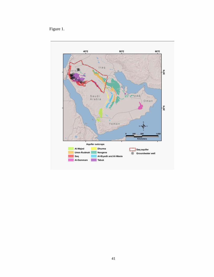
41
Figure 1.
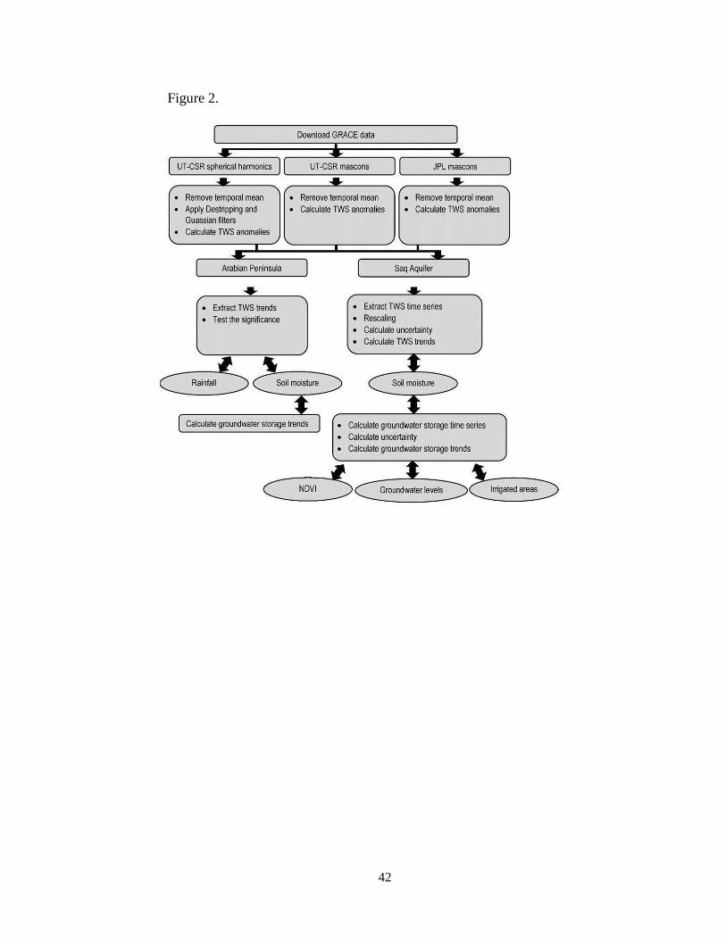
42
Figure 2.
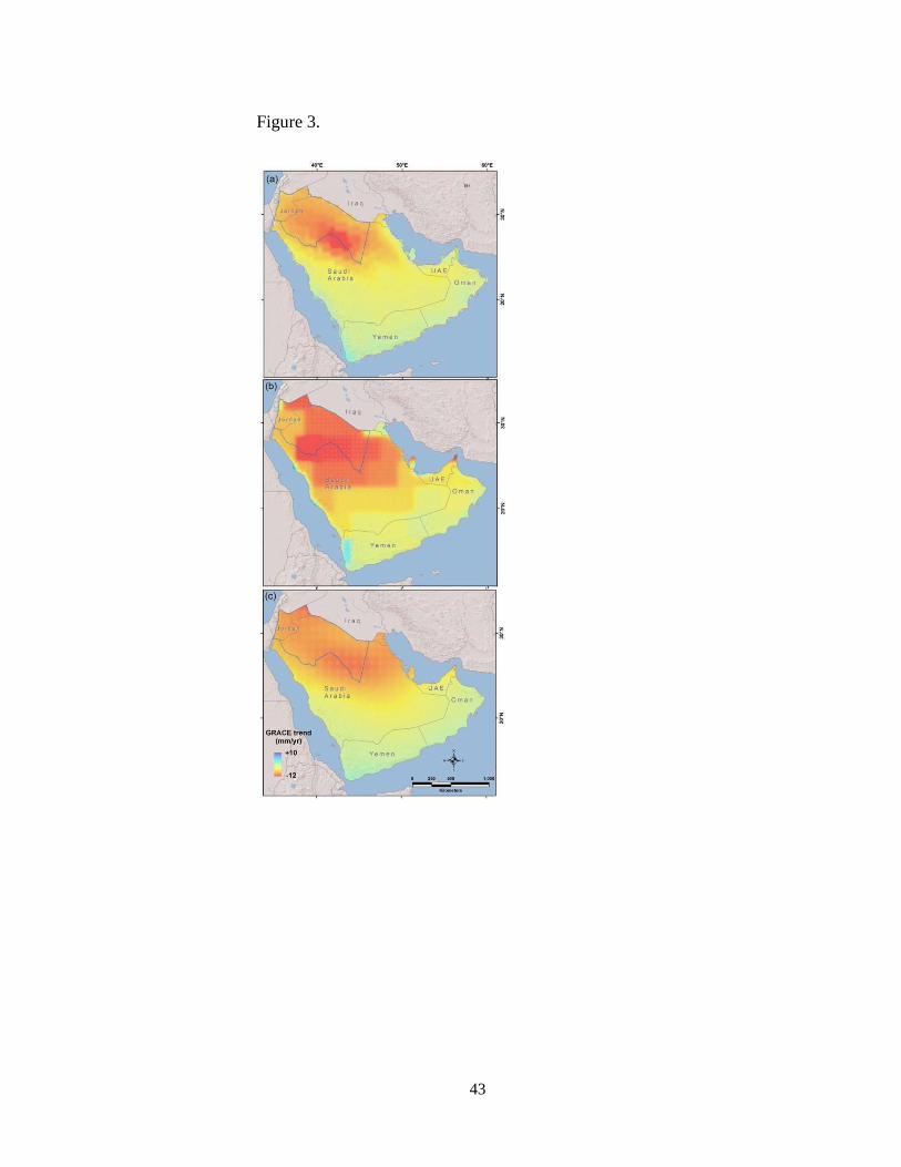
43
Figure 3.
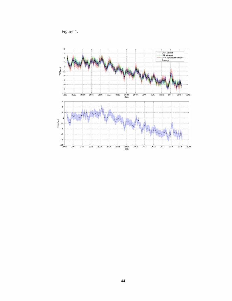
44
Figure 4.
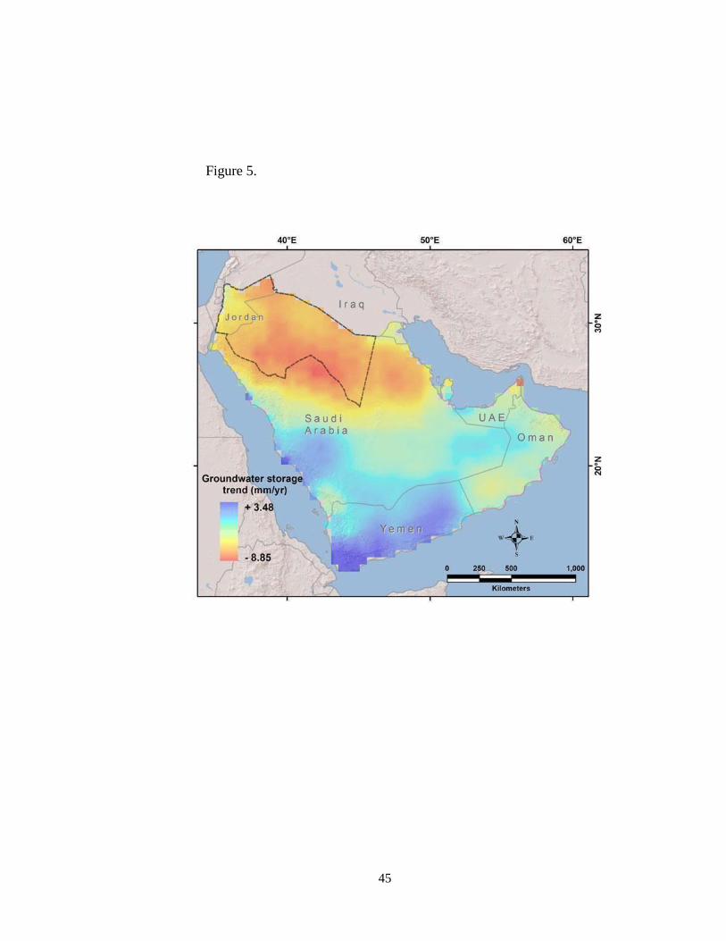
45
Figure 5.
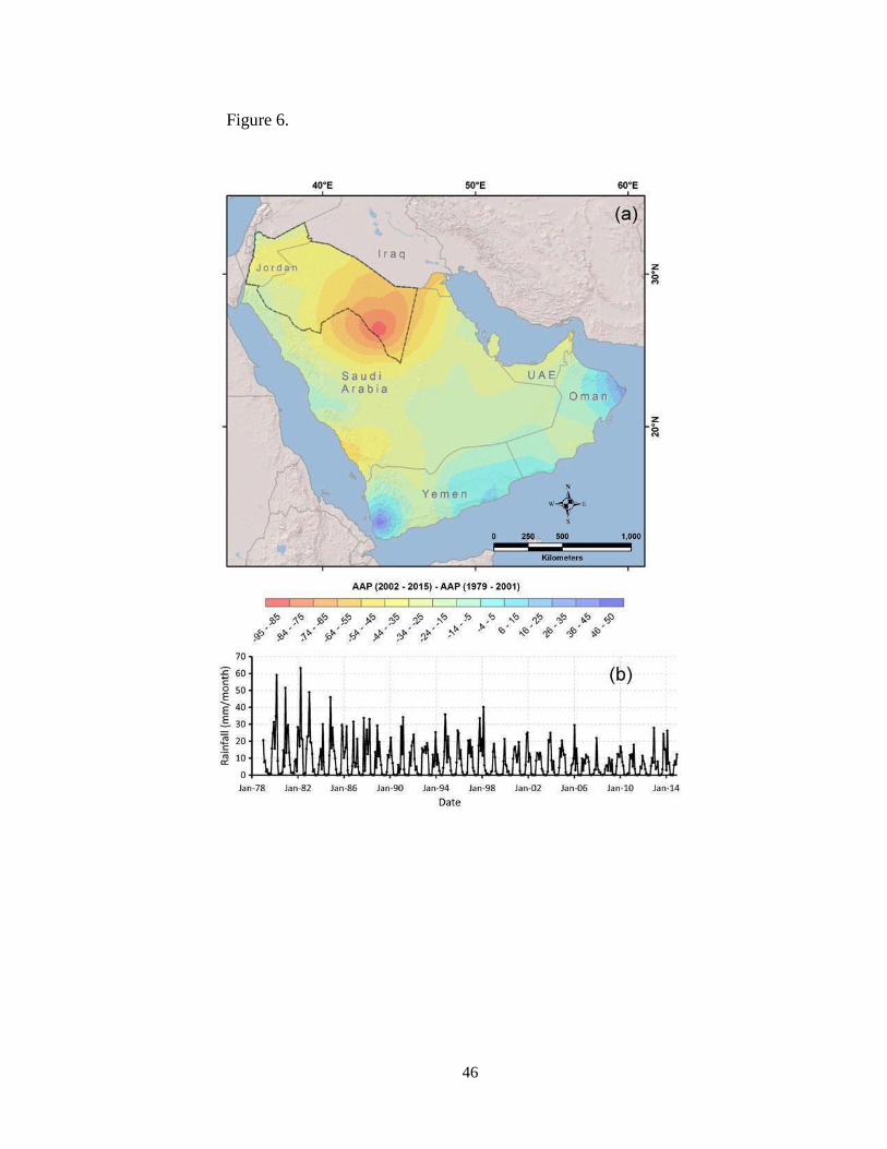
46
Figure 6.

47
Figure 7.
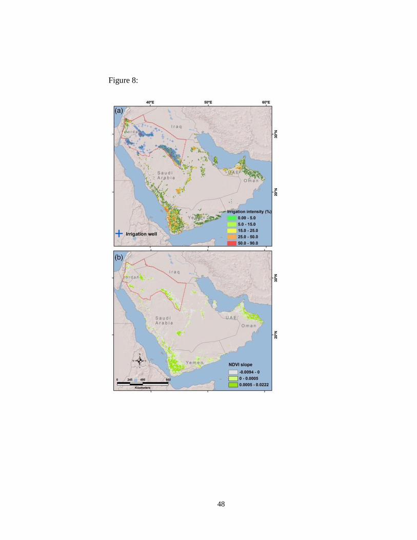
48
Figure 8:
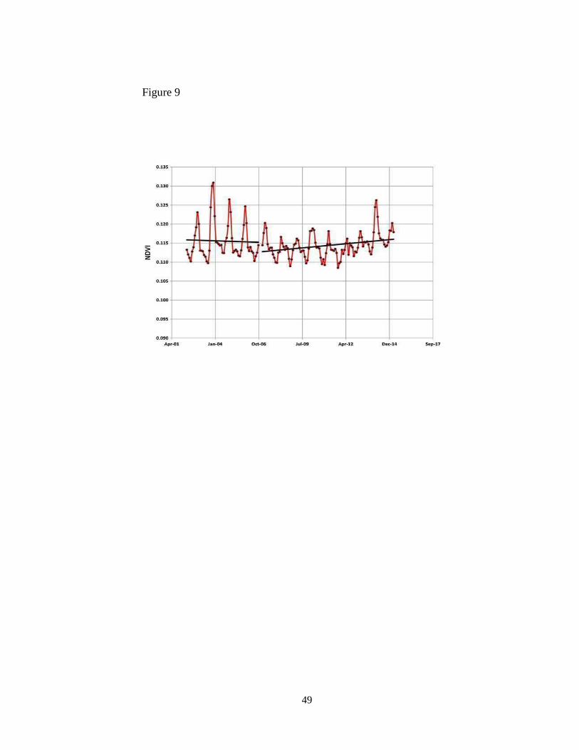
49
Figure 9
50
Manuscript II
Submitted to Journal of Hydrology, 2018
Assessment of Critical Modern Recharge to
Arid Region Aquifer Systems Using an
Integrated Geophysical, Geochemical, and
Remote Sensing Approach
Othman Abdurrahman Fallatah1, 2, Mohamed Ahmed3, 4,
Dawn Cardace5, Thomas Boving1, 5, Ali S. Akanda1
1) Department of Civil and Environmental Engineering, University of
Rhode Island, Kingston, Rhode Island 02881
2) Faculty of Engineering, Radiation Protection & Training Centre, King
AbdulazizUniversity,
P.O. Box 80204, Jeddah 21589, Saudi Arabia
3) Department of Geosciences, Western Michigan University, Kalamazoo,
Michigan 49008
4) Department of Geology, Faculty of Science, Suez Canal University,
Ismailia 41522, Egypt Department of Geosciences, University of Rhode
Island, Kingston, Rhode Island 02881
51
1. Abstract
The arid and semi-arid regions of the world are facing limited freshwater
resources, minimal amounts of rainfall, and increasing population and
water demands. These resources, often groundwater, are vulnerable to
both natural variability and anthropogenic interventions. Here, we
develop and apply an integrated approach using geophysical,
geochemical, and remote sensing observations to quantify the recharge
rates of arid region aquifers that are witnessing rapid groundwater
depletion. Focusing on the Saq aquifer system in the Arabian Peninsula,
our study was three-fold: (1) to examine the areal extent of the aquifer
recharge domains using geologic, climatic, and remote sensing data; (2)
to investigate the origin of, and modern contributions to the aquifer
system by examining the isotopic composition of groundwater samples;
and (3) to estimate the magnitude of contemporary recharge to the aquifer
utilizing Gravity Recovery and Climate Experiment (GRACE) data and
also applying a continuous rainfall-runoff model, the Soil and Water
Assessment Tool (SWAT) model. Isotopic examination of the
groundwater samples from Saq revealed that deeper aquifers (fossil
water) are more depleted compared to shallow reserves (alluvial aquifer;
mixed waters). Analysis of GRACE-derived Terrestrial and groundwater
storage time series indicates that the aquifer system received an annual
recharge rate of 5.21 ± 0.10 km3/yr (11.85 ± 0.22 mm/yr), equal to about
half of groundwater withdrawal rate from wells during the investigation
52
period (April 2002 – December 2016). Analysis of SWAT results
indicates that, during the period from 1998 to 2014, the investigated
watersheds received an average annual precipitation of 19.20 km3, of
which approximately 51% is partitioned as potential recharge. The
temporal variations in storage, depletion, and recharge rates are related to
the changes in regional groundwater extraction, rainfall, and extent of
irrigated areas.
Keywords: Saudi Arabia; Saq Aquifer; Recharge; Soil and Water
Assessment Tool; Gravity Recovery and Climate Experiment; Depletion
53
2. Introduction
The arid and semi-arid parts of the world are currently facing more
difficult problems than ever before when it comes to freshwater resources.
The limited freshwater resources, minimal amounts of rainfall, drought,
and increasing population and living standards are contributing to
environmental and economic devastation in these areas. The freshwater
resources of Saudi Arabia, for example, are primarily those found in
groundwater aquifer systems; only about 5% comes from desalination
plants (Ouda, 2013). These limited resources are extremely vulnerable to
both natural interventions (e.g., rainfall/temperature patterns, duration, and
magnitude) and anthropogenic ones (e.g., population growth, over-
exploitation, and pollution). The average annual rainfall (AAR) over the
entirety of Saudi Arabia decreased from 75 mm in 1930 to 65 mm in 1990,
52 mm in 2000, and 60 mm in 2015. Recent studies have projected that
mean evaporation in that country will increase from 245 mm/yr in 2011 to
368 mm/yr by 2050 (Chowdhury and Al- Zahrani, 2015). On the other
hand, the population growth of Saudi Arabia (1960: 4.0 × 10⁶; 1975: 6.9×
106; 2010: 27.3 × 10⁶) has resulted in a significant increase in freshwater
use. For example, the consumption of freshwater resources in Saudi Arabia
was estimated at 17.9 × 10⁹ m3 in 2010 but expected to be 19.5 × 10⁹ m3
in 2050 (MEWA, 2016). To reduce the pressures on non-renewable
groundwater resources, Saudi Arabia is currently adopting a strategy that
54
introduces advanced irrigation techniques, reduces water-intensive
agricultural production, and uses more desalinated and treated wastewater
and renewable groundwater resources. However, more actions are required
to makeuse the water resources of Saudi Arabia more sustainable. The
most crucial task is to quantify the modern recharge to its principal aquifer
systems.
The Saq aquifer represents one of the most significant transboundary
aquifer systems that extends between northern parts of Saudi Arabia and
southwestern Jordan. The Saq aquifer is witnessing groundwater
overexploitation and is showing severe signs of groundwater decline. For
example, a recent study by Fallatah et al., (2017), indicates that the Saq
aquifer system in Saudi Arabia and Jordan is witnessing groundwater
storage depletions of −6.52 ± 0.29 mm/year (−3.49 ± 0.15 km3/year). The
observed depletion is highly correlated with increasing groundwater
extraction for irrigation and observed water level declines (up to 15 m) in
local supply wells. The major recharge events of the Saq aquifer occurred
only during the past wet climatic periods in Pleistocene ( Abouelmagd et al.
2012; Abouelmagd et al. 2014; Bayumi 2008; Sultan et al. 2008; Sultan et
al. 2011; Wagner 2011; Zaidi et al. 2015). However, the Saq aquifer is
currently receiving minimal recharge under present-day climatic conditions.
Quantifying groundwater recharge of the Saq aquifer is thus key to the
sustainable utilization of the groundwater resources in that system.
Groundwater recharge is generally assessed either by direct or by indirect
55
methods (e.g., Scanlon et al., 2002). Some of the physical and chemical
methods that are used to quantify the recharge are difficult to apply, given
the sizeable areal extent of the Saq aquifer and the absence of field data that
is required for implementing these methods.
In this manuscript, we develop and apply an integrated approach to quantify
the recharge rates of the Saq aquifer system. Given the areal distribution of
the Saq transboundary aquifer system, the interaction between the Saq
aquifer and the overlying aquifers was also assessed. Specifically, we set
out to accomplish the following: (1) examine the areal extent of the Saq
aquifer recharge domains using geologic, climatic, and remote sensing data;
(2) investigate the origin of, and modern contributions to, the groundwater
in the Saq aquifer system by examining the isotopic compositions of
groundwater samples collected from, and outside of, the Saq aquifer; and
(3) estimate, to first order, the magnitude of modern recharge to the Saq
aquifer utilizing data from the Gravity Recovery and Climate Experiment
(GRACE) and applying the continuous rainfall- runoff model, the Soil and
Water Assessment Tool (SWAT).
3. Saq Aquifer System
Saudi Arabia is divided mainly into the Arabian Shield and the Arabian
Shelf. The Arabian Shield, an outcropping along the Red Sea, is principally
composed of Precambrian igneous and metamorphic complexes. On the
other hand, the Arabian Shelf is mainly formed of a sedimentary sequence
lying unconformable on the Arabian Shield and dipping away towards the
56
Arabian Gulf (Fig. 1). The Saq aquifer system is situated in an arc directly
over the Precambrian Arabian Shield, which dips and thickens towards the
Arabian Gulf. This aquifer is characterized by a thick sedimentary
succession of Cambro-Ordovician medium to coarse sandstone that is
unconfined towards the recharge domains and becomes confined towards
the discharge domains. Precipitation that falls along the foothills of the Red
Sea hills feeds the Saq aquifer, and the groundwater flows from the west
towards the east, draining naturally in and close to the Arabian Gulf
(Alsharhan and Nairn 1997; Alsharhan 2001; Alsharhan 2003; Sultan et al.
2008). The water- bearing layer of the Saq aquifer exhibits a large
thickness (400–1200 meters) and high storage capacity (storage: 258 km3;
Abunayyan Trading Corporation and BRGM 2008). The Saq aquifer waters
are believed to have originated, to a great extent, from paleo-precipitation
during the previous wet climatic periods, which recharged the aquifers
through outcrop locations at the foothills of the Red Sea hills (Beaumont
1977; Bayumi 2008; Sultan et al. 2008; Sultan et al. 2011; Wagner 2011;
Abouelmagd et al. 2012; Abouelmagd et al. 2014; Zaidi et al. 2015).
4. Delineating the recharge domains of the Saq aquifer
Two main peak periods characterize seasonal rainfall patterns over Saudi
Arabia. The first peak comes during March and April, followed by almost
no rainfall during June to August, which in turn is followed by a second
peak from October to January. These precipitation events act as the main
sources of recharge to the underlying aquifer systems. Recharge domains of
57
the Saq aquifer system were defined as those areas that are witnessing
annual rainfall and covered by the Saq outcrops. We examined the AAR
data over the Saq aquifer using satellite-based rainfall estimates given the
lack of rain gauges over the monitored area and the discontinuous nature of
rainfall records of the existing stations. The Tropical Rainfall Measuring
Mission (TRMM; version 3B43) dataset (available at
http://mirador.gsfc.nasa.gov/cgi-
bin/mirador/presentNavigation.pl?project=TRMM&tree=project) were
used in this study. TRMM is a joint mission between NASA and the
National Space Development Agency (NASDA) of Japan, launched in
1997. It provides near-global (50°N–50°S) data on rainfall every 3 hours
with a spatial resolution of 0.25° × 0.25° (Huffman et al. 2007). Previous
studies have demonstrated that, over arid and semi-arid regions, TRMM-
derived rainfall estimates provide adequate spatial and temporal
correspondence with steady rainfall and streamflow data (e.g., Adeyewa
and Nakamura 2003; Dinku et al. 2007, 2008; Beighley et al. 2011; Sylla et
al. 2013). The AAR over the entirety of Saudi Arabia is shown in Figure 2.
Examination of Fig. 2 shows that the precipitation is mostly concentrated
over the southern parts of the Red Sea Hills. Generally, over Saudi Arabia,
the precipitation increases from north to south. For example, western and
southwestern areas of Jizan, Asir, Al Bahah, and Makkah receive average
rainfall of up to 300 mm. Al Qasim and the northern parts of the Ar Riyad
and Ash Sharqiyah have an average rainfall of up to 125 mm.
58
Areas that receive average annual rainfall ≥15 mm within the Saq aquifer
domains are believed to represent recharge domains of the Saq aquifer
given the fact that individual precipitation events of <5 mm over arid and
semi-arid areas would produce negligible recharge and/or runoff events
(Mohamed et al., 2016; Milewski et al., 2009). It is worth mentioning that
the Saq aquifer could also receive recharge through the downward and
upward flows from the overlying and underlying aquifer systems,
respectively. The mechanism of this recharging process could, for example,
be through different fault systems existing in the domain (e.g., Sultan et al.,
2007). The recharge domain of the Saq aquifer is shown as the hatched area
in Fig. 2.
5. Geochemical Constraints on the Modern Recharge of the Saq aquifer
The origin of the groundwater in the Saq aquifer, as well as the recharge
timing, are determined from analysis of the isotopic composition of
groundwater samples collected from the aquifer. Twenty-four groundwater
samples, locations shown in Fig. 1, were collected in high-density
polyethylene bottles, which were then tightly capped, and transported from
Saudi Arabia to the United States. The hydrogen (H) and oxygen (O)
isotopic ratios of water samples were analyzed by wavelength scanned
cavity ring-down spectrometry on un-acidified samples by a Picarro L-
1102i WS-CRDS analyzer (Lehmann et al., 2009) at the University of
Massachusetts, Amherst. Samples were vaporized at 110ºC. International
reference standards (IAEA, Vienna, Austria) were used to calibrate the
59
instrument on the VSMOW-VSLAP scale, and working standards were
used with each analytical run. Long-term averages of internal laboratory
standard analytical results yield an instrumental precision of 0.51‰ for δ2H
and 0.08‰ for δ18O. The house reference standards for this particular run
were an instrumental precision of 1.03‰ for δ2H and 0.16‰ for δ18O.
Hydrogen and oxygen stable isotope ratios are reported using conventional
delta (δ) notation, in units of per mil (‰) deviation relative to the Vienna’s
standard mean ocean water (V-SMOW) and PeeDee Belemnite (PDB)
standards (Coplen 1996), where:
δ, ‰ = [(Rsample / Rstandard) − 1]× 103 (1)
and where R = 2H/1H or 18O/16O and the standard is Vienna Standard Mean
Ocean Water (Coplen, 1996).
The isotopic analyses of the collected groundwater samples are listed in
Table 1. Two of these samples are collected from irrigation wells; the
remaining samples are collected from domestic wells. The examined wells
are tapping the Saq and the alluvial aquifer systems. The O and H stable
isotopic ratio of the collected groundwater samples are shown in Figure 3.
Examination of Fig. 3 and Table 1 reveals two main groups of groundwater
samples. Group (I) groundwater samples are collected from wells tapping
the Saq aquifer system (sample ID: 1–12; well depth: 144–607 m), whereas
the Group (II) samples are collected from wells tapping the alluvial aquifer
60
system (sample ID: 13–24; well depth: 12–150 m). The hydrogen (δ2H) and
oxygen (δ18O) isotopic compositions of the groundwater samples collected
from the Saq aquifer (Group I) are more depleted (δ2H: −16.92‰ to
−46.37‰; δ18O: −3.64‰ to −6.05‰) compared to those collected from the
alluvial aquifer system (δ2H: −10.36‰ to +1.38‰; δ18O: 2.96‰ to
+0.10‰). Isotopic compositions of Group I samples could represent either
high elevation recharge from mountainous areas or the Red Sea Hills,
and/or recharge formed mainly of paleo-water "fossil water" precipitated
during moist climate intervals of the late Pleistocene. The fossil water
hypothesis is more acceptable to us given the fact that the isotopic
composition of the most depleted sample (ID: 10; δ2H: −46.37‰; δ18O:
−6.05‰) is similar to that of the fossil water samples collected from similar
geological, environmental, and climatic settings (δ2H: −72‰ to −81‰;
δ18O: −10.6‰ to −11.9‰; Sultan et al., 1997, 2011).
The δ2H and δ18O isotopic compositions of Group II samples and the rest of
the Group I samples represent various degrees of mixing between two
endmembers, one being fossil waters (ID: 10; δ2H: −46.37‰; δ18O:
−6.05‰) and the other being modern precipitation (δ2H: +16.70‰; δ18O:
+0.37‰). This hypothesis is supported by the observed progressive
depletion in the isotopic composition with distance from the recharge areas.
For example, within Group (I), the isotopic compositions of the
groundwater samples collected from, and/or close to, the recharge areas
cropping out at the foothills of the basement outcrops (e.g., sample 9) are
61
less depleted compared to those collected away from the recharge areas
(e.g., sample 10).
6. Quantifying Modern Recharge to the Saq Aquifer
Two independent approaches were used to quantify the amounts and timing
of modern recharge to the Saq aquifer. The first one is based on the
analysis of GRACE data, whereas the second approach focused on rainfall-
runoff modeling using the SWAT model was utilized.
(A) Modern Recharge to the Saq Aquifer: GRACE Constraints
GRACE is a joint NASA/DLR mission that was launched in March
2002 to map the Earth’s static and temporal global gravity fields
(Tapley et al. 2004). The variability in Earth’s gravity field is directly
related to the spatiotemporal variations in the total vertically integrated
terrestrial water storage (TWS; Wahr et al., 1998). The GRACE-
derived Terrestrial Water Storage (TWS) is used
extensively in hydrology, oceanology, cryosphere, and solid Earth
fields (e.g., Ahmed et al. 2011; Famiglietti and Rodell 2013; Ahmed et
al. 2014; Wouters et al. 2014; Famiglietti 2014; Ahmed et al. 2016;
Mohamed et al. 2016).
In this study, the monthly (April 2002 to December 2016) mass
62
concentration (mascons; release 05; version 1; 0.5 º × 0.5º grid)
GRACE-derived TWS solutions generated by the University of Texas
Center for Space Research (UT-CSR) were used. Previous work has
demonstrated that the mascon solutions provide higher signal-to-noise
ratio, higher spatial resolution, and reduced error compared to other
solutions (e.g., spherical harmonics) and do not require spectral (e.g.,
describing) and spatial (e.g., smoothing) filtering or any empirical
scaling techniques (Luthcke et al. 2013; Watkins et al. 2015; Save et al.
2016; Wiese et al. 2016; Scanlon et al. 2016). The UT- CSR mascon
solutions approach uses the geodesic grid technique to model the
surface of Earth using an equal area gridded representation of the planet
via 40,962 cells (40,950 hexagons + 12 pentagons; Save et al. 2012;
Save et al. 2016).
The GRACE-derived TWS time series, generated by spatially
averaging all TWS results over the Saq aquifer, is shown in Figure 4a.
Errors associated with monthly TWS as well as calculated trend values
were then estimated (Tiwari et al. 2009; Scanlon et al. 2016). First, we
fitted the monthly TWSGRACE time series using trend, and we
calculated the seasonal terms and set residuals. We then smoothed these
residuals using a 13-month moving average and removed the trend to
calculate a second set of residuals. Next, we performed Monte Carlo
simulations by fitting trends and seasonal terms for 10,000 synthetic
monthly datasets, each with values chosen from a population of
63
Gaussian-distributed numbers having a standard deviation similar to
that of the second set of residuals. Finally, the standard deviation of the
extracted synthetic trends was interpreted as the trend error for the
GRACE-derived TWS.
We estimated secular trends by simultaneously fitting a trend and
seasonal terms (e.g., annual and semiannual) to the GRACE-derived
TWS time series. The extracted trend values were then statistically
tested adapting the Student’s t-test. The GRACE-derived TWS trend
for the entire period (April 2002 to December 2016) is estimated at
−8.55 ± 0.22 mm/yr (−3.76 ± 0.10 km3/yr). Moreover, piecewise trend
analysis of the GRACE-derived TWS is conducted over three
distinctive periods: April 2002 to March 2006 (Period I), April 2006 to
June 2012 (Period II), and July 2012 to December 2016 (Period III).
The trend results, along with their statistical significance, are shown in
Table 2. Examination of Fig. 4a and Table 2 shows that the Saq aquifer
is witnessing a near-steady state in GRACE-derived TWS during
Period I (Period I: −0.73 ± 0.95 mm/yr [−0.32± 0.42 km3/yr]), a severe
decline in GRACE-derived TWS during Period II (Period II: −11.05
±0.44 mm/yr [−4.86 ± 0.19 km3/yr]), and a modest decrease in
GRACE-derived TWS during Period III (Period III: −4.04 ± 1.62
mm/yr [−1.78 ± 0.71 km3/yr]). The temporal variability in GRACE-
derived TWS is related to temporal variations in one or more of the
TWS compartments (e.g., soil moisture and groundwater).
64
Given the fact that GRACE cannot distinguish between anomalies
resulting from different components of TWS (e.g., soil moisture and
groundwater), the contributions of soil moisture storage need to be
quantified and removed from GRACE-derived TWS (Fig. 4a) to
calculate groundwater storage (GWS). Soil moisture data were
extracted from the Global Land Data Assimilation System (GLDAS).
GLDAS is a NASA-developed land surface modeling system which
performs advanced simulations of climatic and hydrologic variables
using field and satellite-based observations (Rodell et al. 2004). The
GLDAS model simulates soil moisture through four model versions:
VIC, CLM, Noah, and Mosaic (Koster and Suarez 1996; Liang et al.
1996; Koren et al. 1999; Dai et al. 2003; Rodell et al. 2004). The soil
moisture time series (Fig. 4b) over the Saq aquifer was calculated by
averaging the soil moisture estimates from the four GLDAS model
versions. The soil moisture monthly errors were calculated as the mean
monthly standard deviation from the four GLDAS model simulations
(e.g., Tiwari et al. 2009; Voss et al. 2013; Castle et al. 2014; Joodaki et
al. 2014). Trends in soil moisture time series were quantified using the
same approach used for GRACE-derived TWS data.
Fig. 4b shows that the GLDAS-derived soil moisture estimate is
witnessing an overall depletion of −2.21 ± 0.07 mm/yr (−0.97 ± 0.03
km3/yr) during the entire investigated period (April 2002 to December
2016). Inspection of piecewise trend analysis results (Table 2) indicates
65
that the GLDAS-derived soil moisture estimate is always declining
during the three investigated periods but at varying rates (Period I:
−3.23 ± 0.27 mm/yr [−1.42 ± 0.12 km3/yr]; Period II: −2.13 ± 0.13
mm/yr [−0.94 ± 0.06 km3/yr]; Period III: −0.94 ± 0.23 mm/yr [−0.41 ±
0.10 km3/yr]).
The GRACE-derived GWS time series over the Saq aquifer (Fig. 4c) is
generated by subtracting the GLDAS-derived soil moisture storage
(Fig. 4b) from the GRACE-derived TWS (Fig. 4a). The monthly GWS
uncertainties were calculated by summing, in quadrature, the
contributions from GRAC-derived TWS errors to GLDAS-derived soil
moisture errors. Trends in GWS time series were quantified using the
same approach used for GRACE-derived TWS data.
Inspection of Fig. 4c shows that the Saq aquifer is witnessing an overall
GWS decline of −6.34 ± 0.22 mm/yr (−2.79 ± 0.10 km3/yr). Piecewise
trend analysis results (Table 2) shows that the Saq aquifer is
experiencing a GWS increase (+2.50 ± 0.92 mm/yr; +1.10 ± 0.40
km3/yr) during Period I, followed by a sharp GWS decrease (−8.92 ±
0.41 mm/yr; −3.92 ± 0.18 km3/yr) during Period II, then a modest
GWS decline during period III (−3.10 ± 1.59 mm/yr; −1.36 ± 0.70
km3/yr).
To quantify the recharge rates during the investigated periods, we
added the summation of natural discharge and anthropogenic
groundwater extraction to the GWS trends utilizing the following
66
equation:
𝑅𝑒𝑐ℎ𝑎𝑟𝑔𝑒 = ∆𝐺𝑊𝑆 + 𝐷𝑖𝑠𝑐ℎ𝑎𝑟𝑔𝑒 (𝑛𝑎𝑡𝑢𝑡𝑎𝑙𝑛𝑎𝑡𝑢𝑟𝑎𝑙 +
𝑎𝑛𝑡ℎ𝑟𝑜𝑝𝑜𝑔𝑒𝑖𝑐𝑟𝑜𝑝𝑜𝑔𝑒𝑛𝑖𝑐). (2)
The discharge rate of the Saq aquifer system over the last decade was
estimated at ~8.00 km3/yr (18.20 mm/yr; Sultan et al. 2007; Mohamed
et al. 2016). Following Equation 2, the recharge rate for the Saq
aquifer is estimated at 5.21 ± 0.10 km3/yr (11.85 ± 0.22 mm/yr) during
the entire investigated period. The recharge rate of the Saq aquifer
during Periods I, II, and III is estimated at 9.10 ± 0.40 km3/yr, 4.08 ±
0.18 km3/yr, and 6.64 ± 0.70 km3/yr, respectively.
The temporal variations in GRACE-derived TWS and GWS are
related to the temporal variations in groundwater extraction rates and
irrigated areas (e.g., Fallatah et al., 2017; Ahmed et al., 2016). For
example, the total areas for the irrigated lands decreased from 3.56 x
106 hectares during the period from 2000 to 2006 to 2.76 x 10⁶
hectares during the period from 2006 to 2012 (MEWA, 2016).
Moreover, the variations in recharge rates of the Saq aquifer during the
investigated periods are related to the temporal variations in
groundwater extraction and rainfall rates. The AAR was estimated at
79 mm, 51 mm, and 75 mm during Periods I, II, and III, respectively.
Examination of AAR and recharge rates over the Saq Aquifer shows
an obvious correspondence of the recharge rates on the rainfall
amounts. It is worth mentioning that a one-to-one correspondence, in
67
magnitudes between recharge and AAR, is not to be expected, given
that AAR could be redistributed as runoff and evapotranspiration that
could affect the spatial and temporal distribution of the precipitated
water, and hence the recharge locations and magnitudes.
(B) Modern Recharge to the Saq Aquifer: Modeling Constraints
The modern recharge of the Saq aquifer was quantified using SWAT, a
catchment-based, semi- distributed hydrologic model that was
developed for continuous simulation of surface runoff and potential
recharge to the groundwater system. Among other things, the SWAT
model simulates overland flow, channel flow, transmission losses,
evaporation and evapotranspiration, and potential recharge (Arnold &
Fohrer, 2005; Arnold, Srinisvan, Muttiah, & Williams, 1998). SWAT
has been used to quantify the recharge rates in similar geologic
environments and settings, including but not limited to the Eastern
Desert (Milewski et al., 2009) and Sinai Peninsula(Sultan et al., 2011)
of Egypt, the Saudi Red Sea watersheds (Sultan et al., 2015), and
Kuwait (Aldosari et al., 2010).
In our simulations, the SWAT model used the US Department of
Agriculture Soil Conservation Service method (SCS, 1972) to quantify
the initial losses and direct overland flows. We estimated channel
flows using the Muskingum routing method (McCarthy, 1938), and we
used Manning’s coefficient for uniform flow in a channel to calculate
68
the rate and velocity of flow in a reach segment for a given time step.
Evaporation was estimated using the Penman-Monteith method
(Monteith, 1981).
The SWAT model climatic inputs include rainfall, minimum and
maximum temperature, solar radiation, relative humidity and wind
speed. The climatic data were extracted from the Global Weather Data
(GWD) for SWAT database (available at
http://globalweather.tamu.edu/). The GWD-derived rainfall data was
validated against available rain gauge records. A comparison between
monthly GWD-derived rainfall records and the available rain gauges is
shown in Figure 5. Locations of the selected rain gauges are
shown in Figure 6. Examination of Fig. 5 reveals satisfactory general
correspondence (R2: 0.72 to 0.85) between the average monthly
rainfall measured in the field and that obtained from GWD. We should
note that a one-to-one correspondence between GWD and gauge-
derived rainfall measurements is not expected given the fact that GWD
integrates measurements over a large area (~ 38 km × 38 km).
The SWAT topographic data input was extracted from the Shuttle
Radar Topography Mission (SRTM)-derived Digital Elevation Model
(DEM; spatial resolution: 90 m; available at http://dwtkns.com/srtm/).
The SWAT model uses the DEM data to delineate watersheds, extract
channel networks, and calculate the morphometric parameters (e.g.,
slope angle, channel slope, channel length and channel width, etc.).
69
The soil data inputs for SWAT model were extracted from Saudi
Arabia geological maps (SGS, 1990). Five main soil types were
recognized in the study area: alluvial sediments, sandstone, shale,
limestone, and basement rocks. The land use data were extracted from
the Global Land Cover 30-meter database (available at
(http://www.globeland30.org/GLC30Download/index.aspx).
SWAT simulations were performed at daily time steps for the period
from 1998 to 2014 given the input GWD data availability. A manual
calibration routine was applied to calibrate the SWAT model utilizing
the model parameters used in Sultan et al. (2015). Several approaches
have been applied to calculate the recharge rates out of the SWAT
model in similar geologic, environmental, and climatic settings. For
example, Al-Dousari et al. (2010) estimate the recharge as the
summation of transmission losses and 5% of the initial losses;
Milewski et al. (2009) and Sultan et al. (2011) used the transmission
losses as a recharge rate; Milewski et al. (2014) assumed that the
recharge rate equals the initial losses. In this study, we’ve adapted the
approach of Sultan et al. (2015) to calculate potential recharge rates of
the investigated watersheds.
Table 3 lists the model results for the four investigated watersheds.
Streamflow was calculated by subtracting the transmission losses from
the summation of surface runoff, lateral flow, and return flow. The
potential recharge, however, was calculated by subtracting the
70
summation of amounts of water moving from shallow aquifers to
plants/soil by re-evaporation (Revap) and return flow from the
summation of percolation to shallow aquifer and transmission losses.
Finally, the initial losses were estimated by subtracting the summation
of potential recharge and streamflow from precipitation.
Examination of Table 3 indicates that, during the period from 1998 to
2014, the four investigated watersheds, Al Baten, Al Rumah, Al
Sarhan, and Tabuk, shown in Fig. 6, received average annual
precipitation of 19.20 km3. Of this precipitation, an average of 9.83
km3 (51% of the total rainfall) is partitioned as potential recharge. It is
worth mentioning that by increasing the proportion of areas occupied
by basement and/or rising precipitation amounts, the stream flow
proportion is increased. Moreover, the higher the amount of
precipitation and the stream flow, the higher the amount of potential
recharge.
7. Sustainable Utilization and Management of the Saq Aquifer
System
GRACE-based average annual groundwater recharge to the Saq aquifer
system during the period from April 2002 to December 2016 was
estimated at 5.21 ± 0.10 km3, assuming a constant average yearly
groundwater extraction amount of 8.00 km3. Moreover, the SWAT-
based average annual groundwater recharge during the period from
71
January 1998 to December 2014 was estimated at 9.83 km3. The
difference between the recharge rates calculated from the two
independent sources might be related to one or more of the following:
(1) variation in the spatial extent of the examined areas (GRACE area:
0.43 x 10⁶ km2; SWAT area: 0.37 x 10⁶ km2), (2) difference in the
monitored time periods (GRACE: April 2002 to December 2016;
SWAT: January 1998 to December 2014), or (3) difference in the
approach used to calculate recharge in each technique.
Sustainable utilization and management of the water resources of the Saq
aquifer system could be achieved by adopting the following practices.
First, groundwater extraction areas should be located at, or near to, the
center of the aquifer; areas around the aquifer borders are expected to be
depleted first as extraction increases with time. Second, groundwater
extraction rates should be limited to maintain the GWS trend at ≥0;
positive GWS trends means the extraction is less than the recharge, zero
GWS trend implies extraction equals recharge, and negative GWS trends
implies the extraction is greater than the recharge. Third, utilize the well
spacing act such that the effects on the aquifer are not concentrated at any
spot and well yields are sustained. The optimum well spacing is a
function of a total number of wells, aquifer thickness, regional
groundwater velocity, and pumping rate of an extraction well (Ahmed
1995), expressed as:
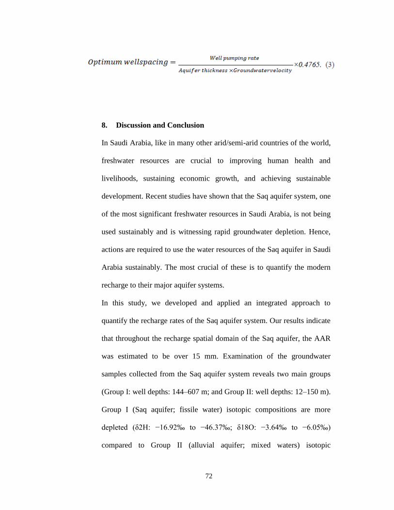
72
8. Discussion and Conclusion
In Saudi Arabia, like in many other arid/semi-arid countries of the world,
freshwater resources are crucial to improving human health and
livelihoods, sustaining economic growth, and achieving sustainable
development. Recent studies have shown that the Saq aquifer system, one
of the most significant freshwater resources in Saudi Arabia, is not being
used sustainably and is witnessing rapid groundwater depletion. Hence,
actions are required to use the water resources of the Saq aquifer in Saudi
Arabia sustainably. The most crucial of these is to quantify the modern
recharge to their major aquifer systems.
In this study, we developed and applied an integrated approach to
quantify the recharge rates of the Saq aquifer system. Our results indicate
that throughout the recharge spatial domain of the Saq aquifer, the AAR
was estimated to be over 15 mm. Examination of the groundwater
samples collected from the Saq aquifer system reveals two main groups
(Group I: well depths: 144–607 m; and Group II: well depths: 12–150 m).
Group I (Saq aquifer; fissile water) isotopic compositions are more
depleted (δ2H: −16.92‰ to −46.37‰; δ18O: −3.64‰ to −6.05‰)
compared to Group II (alluvial aquifer; mixed waters) isotopic
73
compositions (δ2H: −10.36‰ to +1.38‰; δ18O: 2.96‰ to +0.10‰).
Analysis of GRACE-derived TWS and GWS time series indicates that
the Saq aquifer is receiving annual recharge 5.21 ± 0.10 km3/yr (11.85 ±
0.22 mm/yr) during the entire investigated period (April 2002 to
December 2016). Assuming constant groundwater extraction rates (8
km3/yr), the recharge rate of the Saq aquifer is witnessing a temporal
variability. The temporal variations in GRACE-derived TWS, GWS, and
recharge rates are related to the temporal variations in groundwater
extraction rates, rainfall rates, and extent of irrigated regions. Analysis of
SWAT results indicates that, during the period from 1998 to 2014, the
four investigated watersheds (Al Baten, Al Rumah, Al Sarhan, and
Tabuk) received average annual precipitation of 19.20 km3. Of this
precipitation, an average of 9.83 km3 (51% of the total rainfall) is
partitioned as potential recharge.
Our results, we believe, will contribute to the effective and efficient
utilization of the Saq aquifer water resources and will be used to promote
the sustainable development of the Arabian Peninsula's natural resources
in general. This study’s findings are being shared with decision makers in
relevant governmental agencies to develop sustainable management
scenarios for the water resources of the Saq aquifer.
74
9. Acknowledgments
The authors are thankful Ministry of Environment Water and Agriculture in
Saudi Arabia for providing the scientific data to improve this paper. Special
acknowledgments are extended to Ministry of Water Tabuk Branch for
providing all facilities needed to complete this work.
75
10. References
1. Abunayyan, BRGM (2008) Investigations for updating the
groundwater mathematical model(s) of the Saq overlying
aquifers. Ministry of Water and Electricity, Riyadh,Saudi
Arabia. https://www.scribd.com/document/16845648/Saq-
Aquifer-Saudi-Arabia-2008
2. Abouelmagd, A., Sultan, M., Milewski, A., Kehewa, A. E.,
Sturchio, N., Soliman, F., Krishnamurthy, R. V., & Cutrim,
E. (2012). Toward a better understanding of palaeoclimatic
regimes that recharged the fossil aquifers in North Africa:
Inferencesfrom stable isotope and remote sensing data.
Palaeogeography, Palaeoclimatology, Palaeoecology 329–
330, 137–149. doi: 10.1016/j.palaeo.2012.02.024
3. Abouelmagd, A., Sultan, M., Sturchio, N. C.,…Chouinard,
K. (2014). Paleoclimate record in the Nubian Sandstone
Aquifer, Sinai Peninsula, Egypt. Quaternary Research
(United States) 81, 158–167. doi:
10.1016/j.yqres.2013.10.017
4. Adeyewa, Z. D., & Nakamura, K. (2003). Validation of
TRMM radar rainfall dataover major climatic regions in
Africa. Journal of Applied Meteorology 42, 331–347. doi:
10.1175/1520-0450(2003)042<0331:VOTRRD>2.0.CO;2
5. Ahmed, M., Sultan, M., Wahr, J., & Yan, E. (2014). The
76
use of GRACE data to monitor natural and anthropogenic
induced variations in water availability across Africa.
Earth Science Reviews 136:289–300. doi:
10.1016/j.earscirev.2014.05.009
6. Ahmed, M., Sultan, M., Wahr J, Yan, E., Milewski, A.,
Sauck, W., Becker, R., & Welton, B. (2011) Integration
of GRACE (Gravity Recovery and Climate Experiment)
data with traditional data sets for a better understanding
of the time-dependent water partitioning in African
watersheds. Geology 39:479–482. doi: 10.1130/G31812.1
7. Ahmed, M., Sultan, M., Yan, E., & Wahr, J. (2016).
Assessing and improving land surface model outputs over
Africa using GRACE, field, and remote sensing data.
Surveys in Geophysics 37, 529–556. doi:
10.1007/s10712-016-9360-8
8. Ahmed, W. (1995). Optimum spacing of extraction
wells. Hydrogeology 3, 64–74.
9. Al-Dousari, A., Milewski, A., Din, S. U., & Ahmed, M.
(2010). Remote sensing inputs to SWAT model for
groundwater recharge estimates in Kuwait. Advances in
Natural and Applied Sciences, 4(1), 71–77.
10. Alsharhan, A. S., Rizk, Z. A., Nairn, A. E. M., Bakhit, D.
W., & Alhajari, S. A. (Eds.). (2001). Hydrogeology of an
77
arid region: the Arabian Gulf and adjoining areas. Elsevier.
11. Alsharhan, A. S. (2003). Petroleum geology and potential
hydrocarbon plays in the Gulf of Suez rift basin, Egypt.
AAPG bulletin, 87(1), 143-180.
12. Arnold, J. G., & Fohrer, N. (2005). SWAT2000: current
capabilities and research opportunities in applied watershed
modeling. Hydrological Processes, 19(3), 563–572.
13. Arnold, J. G., Srinivasan, R., Muttiah, R. S., & Williams, J.
R. (1998). Large area hydrologic modeling and assessment
part I: model development. Journal of the American Water
Resources Association, 34(1), 73–89.
14. Bayumi, T. (2008). Quantitative Groundwater Resources
Evaluation in the Lower Part of Yalamlam Basin, Makkah
Al Mukarramah, Western Saudi Arabia. Journal of King
Abdulaziz University of Science 19, 35–56. doi:
10.4197/Ear.19–1.3
15. Beaumont, P. (1977). Water and Development in Saudi
Arabia. The Geographical Journal 143, 42. doi:
10.2307/1796674
16. Beighley, R. E., Ray, R. L., He, Y., Shum, C. K.. (2011).
Comparing satellite-derived precipitation datasets using the
Hillslope River Routing (HRR) model in the CongoRiver
Basin. Hydrological Processes 25, 3216–3229. doi:
78
10.1002/hyp.8045
17. Castle, S., Thomas, B., Reager, J., Rodell, M., Swenson, S.
C., & Famiglietti, J. S. (2014). Groundwater depletion
during drought threatens future water security of the
Colorado River Basin. Geophysical Research Letters 10,
5904–5911. doi: 10.1002/2014GL061055.Received
18. Chowdhury, S., & Al-Zahrani, M. (2015). Characterizing
water resources and trends of sector-wise water
consumptions in Saudi Arabia. Journal of King Saud
University- of Engineering Sciences, 27(1), 68–82
19. Coplen, T. B. (1996). New guidelines for reporting stable
hydrogen, carbon, and oxygen isotope-ratio data.
Geochimica et Cosmochimica Acta 60, 3359–3360. doi:
10.1016/0016- 7037(96)00263-3
20. Dai, Y., Zeng, X., Dickinson, R. E., Yang, Z. L. (2003). The
common land model. Bulletin of the American
Meteorological Society 84, 1013–1023. doi:
10.1175/BAMS-84- 8-1013
21. Dinku, T., Ceccato, P., Grover‐Kopec, E., Lemma, M.,
Connor, S. J., & Ropelewski, C. F. (2007). Validation of
satellite rainfall products over East Africa's complex
topography. International Journal of Remote Sensing 28,
1503–1526. doi: 10.1080/01431160600954688
79
22. Dinku, T., Chidzambwa, S., Ceccato, P., Connor, S. J., &
Ropelewski, C. F. (2008). Validation of high‐resolution
satellite rainfall products over complex terrain. International
Journal of Remote Sensing 29, 4097–4110. doi:
10.1080/01431160701772526
23. Famiglietti, J. S. (2014). The global groundwater crisis.
Nature Climate Change 4, 945– 948. doi:
10.1038/nclimate2425
24. Famiglietti, J. S., Rodell, M. (2013). Water in the balance.
Science (80- ) 340, 1300– 1301. doi:
10.1126/science.1236460
25. Fallatah, O. A., Ahmed, M., Save, H., & Akanda, A. S.
(2017). Quantifying temporal variations in water resources
of a vulnerable Middle Eastern transboundary aquifer
system. Hydrological Processes. 2017;1–11.
https://doi.org/10.1002/ hyp.11285
26. Huffman, G. J, Bolvin, D. T., Nelkin, E. J., & Stocker, E. F.
(2007). The TRMM multi- satellite precipitation analysis
(TMPA): Quasi-global, multiyear, combined-sensor
precipitation estimates at fine scales. Journal of
Hydrometeorology 8, 38–55. doi: 10.1175/JHM560.1
27. Joodaki, G., Wahr, J., & Swenson, S. (2014). Estimating the
human contribution to groundwater depletion in the Middle
80
East, from GRACE data, land surface models, and well
observations Gholamreza. Water Resources Research 50, 1–
14. doi: 10.1002/2013WR014633.Received
28. Koren, V., Schaake, J., Mitchell, K., Duan, Q.-Y., Chen, F.,
& Baker, J. M. (1999). A parameterization of snowpack and
frozen ground intended for NCEP weather and climate
models. Journal of Geophysical Research 104, 19569–
19585. doi: 10.1029/1999JD900232.
29. Koster, R. D., & Suarez, M. J. (1996). Energy and water
balance calculations in the Mosaic LSM. National
Aeronautics and Space Administration, Goddard Space
Flight Center, Laboratory for Atmospheres, Data
Assimilation Office: Laboratory for Hydrospheric
Processes.
30. Lehmann, K. K., Berden, G., & Engeln, R. (2009). An
introduction to cavity ring-down spectrometry, in Berden,
G., and Engeln, R., eds., Cavity Ring-Down
SpectrometryTechniques and Applications. London: John
Wiley & Sons Ltd.
31. Liang, X., Lettenmaier, D. P., & Wood, E. F. (1996). One-
dimensional statistical dynamic representation of subgrid
spatial variability of precipitation in the two-layer variable
infiltration capacity model. Journal of Geophysical
81
Research 101, 21403. doi: 10.1029/96JD01448
32. Luthcke, S. B., Sabaka, T. J., Loomis, B. D., Arendt, A. A.,
McCarthy, J. J., & Camp, J. (2013). Antarctica, Greenland,
and Gulf of Alaska land-ice evolution from an iterated
GRACE global mascon solution. Journal of Glaciology 59,
613–631. doi: 10.3189/2013JoG12J147
33. McCarthy, G.T. (1938). The unit hydrograph and flood
routing. Conference of North Atlantic Division, US Army
Corps of Engineers. Providence: Army EngineerDistrict,
Providence.
34. Milewski, A., Sultan, M., Al‐Dousari, A., & Yan, E. (2014).
Geologic and hydrologic settings for development of
freshwater lenses in arid lands. Hydrological Processes,
28(7), 3185–3194.
35. Milewski, A., Sultan, M., Yan, E., Becker, R., Abdeldayem,
A., Soliman, F., & Gelil, K. (2009). A remote sensing
solution for estimating runoff and recharge in arid
environments. Journal of Hydrology, 373(1), 1–14.
36. Ministry of Environment, W. a. A. (Jan 1, 2017).
"Estimated Area and Production by Administrative
Regions.” http://www.data.gov.sa/en/group/agriculture-and-
fishing
37. Mohamed, A., Sultan, M., Ahmed, M., Yan, E., & Ahmed,
82
E. (2016). Aquifer recharge, depletion, and connectivity:
Inferences from GRACE, land surface models,
geochemical, and geophysical data. GSA Bulletin 1–13. doi:
10.1130/B31460.1
38. Monteith, J. L. (1981). Evaporation and surface
temperature. Quarterly Journal of the Royal Meteorological
Society, 107(451), 1–27.
39. Nairn, A. E. M., & Alsharhan, A. S. (1997). Sedimentary
basins and petroleum geology of the Middle East. Elsevier.
40. Ouda, O. K. (2013). Towards an assessment of Saudi Arabia
public awareness of water shortage problem. Resources and
Environment, 3(1), 10–13.
41. Rodell, M., Houser, P. R., Jambor, U.,…Toll, D. (2004) The
global land data assimilation system. Bulletin of the
American Meteorological Society 85, 381–394. doi:
10.1175/BAMS-85-3-381
42. Save, H., Bettadpur, S., & Tapley, B. D. (2016).
High‐resolution CSR GRACE RL05 mascons. Journal of
Geophysical Research: Solid Earth, 121(10), 7547-7569.
43. Save, H., Bettadpur, S., & Tapley, B. D. (2012). Reducing
errors in the GRACE gravity solutions using regularization.
Journal of Geodesy 86, 695–711. doi: 10.1007/S00190-
012-0548-5
83
44. Scanlon, B. R., Healy, R. W., & Cook, P. G. (2002).
Choosing appropriate techniques for quantifying
groundwater recharge. Hydrogeology Journal, 10(1), 18–39.
45. Scanlon, B. R., Zhang, Z., Save, H., Wiese, D. N., Landerer,
F. W., Long, D., Longuevergne, L., & Chen, J. (2016).
Global evaluation of new GRACE mascon products for
hydrologic applications. Water Resources Research 52,
9412–9429. doi: 10.1002/2016WR019494
46. Saudi Geological Survey (SGS). (1990). Geological map of
the main sedimentary rock main types in the eastern and the
northern parts of the kingdom of Saudi Arabia
(http://www.sgs.org.sa/English/Pages/Default.aspx)
47. Sultan, M., Metwally, S., Milewski, A.,…Welton, B.
(2011). Modern recharge to fossil aquifers: Geochemical,
geophysical, and modeling constraints. Journal of
Hydrology 403, 14–24. doi: 10.1016/j.jhydrol.2011.03.036
48. Sultan, M., Sefry, S., & AbuAbdallah, M. (2015). Impacts
of climate change on the Red Sea region and its watersheds,
Saudi Arabia. In The Red Sea (pp. 363–377). Springer:
Berlin.
49. Sultan, M., Sturchio, N., Al Sefry, S., Milewski, A., Becker,
R., Nasr, I., & Sagintayev,
50. Z. (2008). Geochemical, isotopic, and remote sensing
84
constraints on the origin and evolution of the Rub Al Khali
aquifer system, Arabian Peninsula. Journal of Hydrology
356, 70–83. doi: 10.1016/j.jhydrol.2008.04.001
51. Sultan, M., Yan, E., Sturchio, N., Wagdy, A., Abdel Gelil,
K., Becker, R., Manocha, N., & Milewski, A. (2007).
Natural discharge: A key to sustainable utilization of fossil
groundwater. Journal of Hydrology 335, 25–36. doi:
10.1016/j.jhydrol.2006.10.034
52. Sylla, M. B., Giorgi, F., Coppola, E., & Mariotti, L. (2013).
Uncertainties in daily rainfall over Africa: assessment of
gridded observation products and evaluation of a regional
climate model simulation. International Journal of
Climatology 33, 1805–1817. doi: 10.1002/joc.3551
53. Tapley, B. D., Bettadpur, S., Ries, J. C., Thompson, P. F., &
Watkins, M. M. (2004).GRACE measurements of mass
variability in the Earth system. Science 305, 503–505. doi:
10.1126/science.1099192 Tiwari, V. M., Wahr, J., &
Swenson, S. (2009) Dwindling groundwater resources in
northern India, from satellite gravity observations.
Geophysical Research Letters 36, L18401. doi:
10.1029/2009GL039401
54. Voss, K. A., Famiglietti, J. S., Lo, M., de Linage, C.,
Rodell, M., & Swenson, S. C. (2013). Groundwater
85
depletion in the Middle East from GRACE with
implications for transboundary water management in the
Tigris-Euphrates-Western Iran region. Water Resources
Research 49, 904–914. doi: 10.1002/wrcr.20078
55. Wagner, W. (2011). Groundwater in the Arab Middle East.
Springer Science & Business Media.
56. Wahr, J., Molenaar, M., & Bryan, F. (1998). Time
variability of the Earth’s gravityfield: Hydrological and
oceanic effects and their possible detection using GRACE.
Journal of Geophysical Research 103, 30205–30229. doi:
10.1029/98JB02844
57. Watkins, M. M., Wiese, D. N., Yuan, D., Boening, C., &
Landerer, F. W. (2015).Improved methods for observing
Earth's time-variable mass distribution with GRACE using
spherical cap mascons. Journal of Geophysical Research-
Solid Earth 120, 2648– 2671. doi:
10.1002/2014JB011547.Received
58. Wiese, D. N., Landerer, F. W., & Watkins, M. M. (2016).
Quantifying and reducing leakage errors in the JPL RL05M
GRACE mascon solution. Water ResourcesResearch 52,
7490–7502. doi: 10.1002/2016WR019344
59. Wouters, B., Bonin, J. A., Chambers, D. P., et al. (2014).
GRACE, time-varying gravity, Earth system dynamics and
86
climate change. Reports Prog Phys. doi: 10.1088/0034-
4885/77/11/116801
60. Zaidi, F. K., Nazzal, Y., Ahmed, I., Naeem, M., &
KamranJafri, M. (2015). Identification of potential artificial
groundwater recharge zones in Northwestern Saudi Arabia
using GIS and Boolean logic. Journal of African Earth
Science 111, 156–169. doi: 10.1016/j.jafrearsci.2015.07.008
87
Figure Legends:
Figure 1: Location map showing the aerial distribution of major
aquifer outcrops in Saudi Arabia. Also shown are the spatial
domain of the Saq aquifer system (red polygon) and the locations
of the groundwater samples (black crosses) examined in this
study.
Figure 2: AAR (mm) extracted from TRMM over Saudi. Also
shown are the spatial domain of the administrative regions (black
dashed lines), Saq aquifer system (black polygon), Saq outcrop
(black area), and the recharge domains of the Saq aquifer system
(hatched area).
Figure 3: δ2H versus δ18O plot for the groundwater samples
collected from Saq aquifer system. Also shown are the isotopic
composition of modern rainfall and the Global Meteoric Water
Line.
Figure 4: Temporal variations in (a) GRACE-derived TWS
estimates, (b) GLDAS-derived soil moisture estimates, and (c)
GRACE-derived GWS estimates averaged over the Saq aquifer
system in Saudi Arabia. Also shown are the error bars in each
time series.
88
Figure 5: Comparison between average monthly rainfall estimates
reported from rain gauges and GWD-derived estimates. The
degree of fitness, R2, is also shown for each plot.
Figure 6: The spatial distribution of the four watersheds examined
by the SWAT model overlying the SRTM-derived DEM. Also
shown are the GWD network and the spatial distribution of the six
rain gauges shown in Fig. 5.
89
Tables captions:
Table 1: Well information and O and H isotopic compositions for
groundwater samples collected from the Saq aquifer system in
Saudi Arabia.
Table 2: Trends in water budget components averaged over the Saq
aquifer system during the investigated period (April 2002 to
December 2016). Trends that are significant at ≥65% level of
confidence are underlined and at ≥95% level of confidence are
normal.
Table 3: SWAT model results for the four investigated watersheds
during the period from 1998 to 2014.
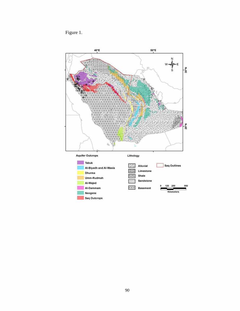
90
Figure 1.
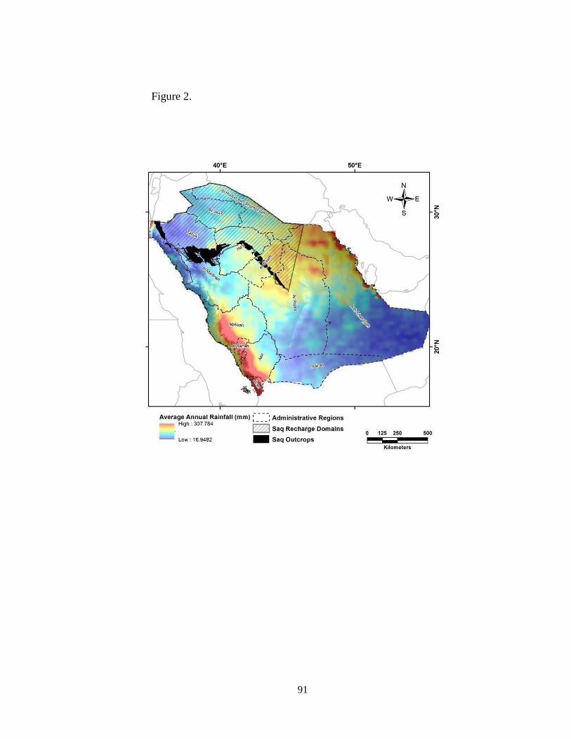
91
Figure 2.
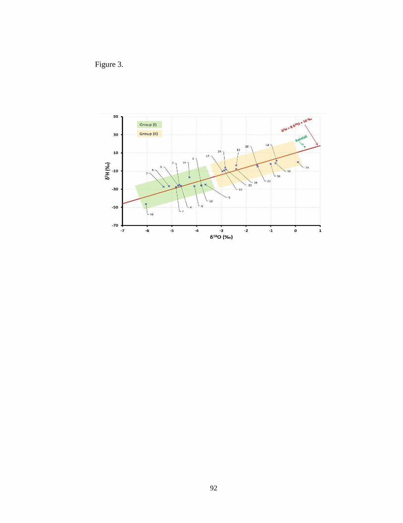
92
Figure 3.
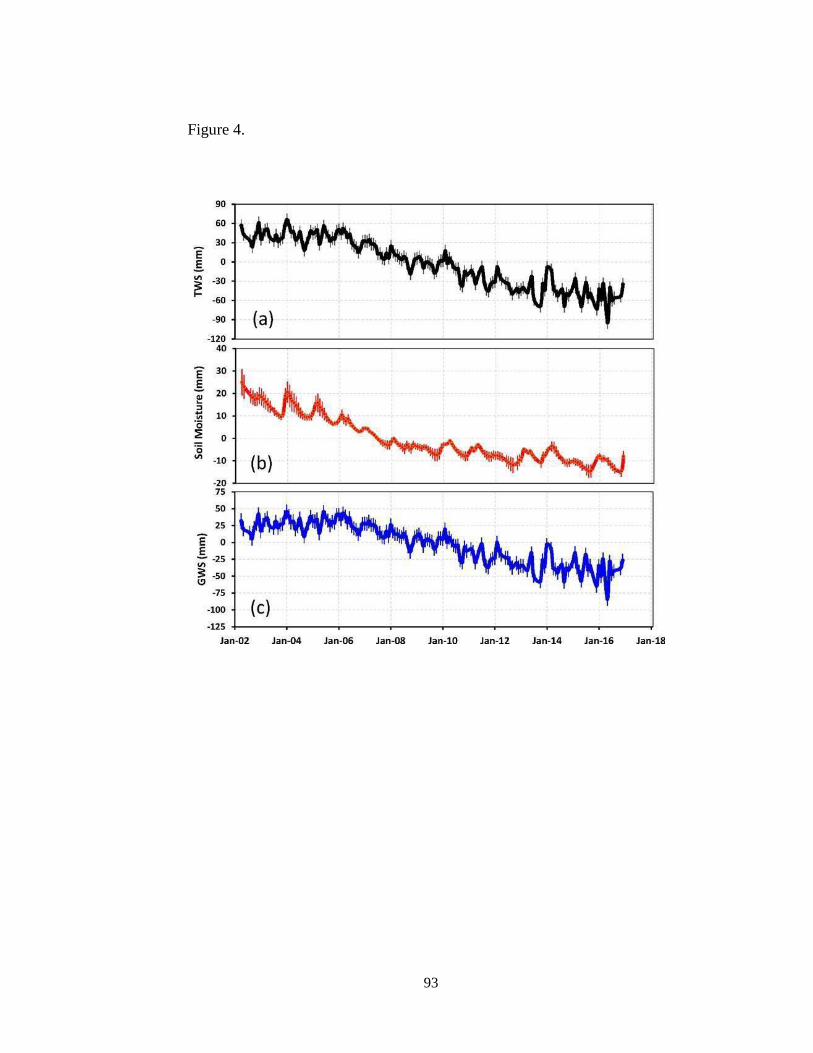
93
Figure 4.
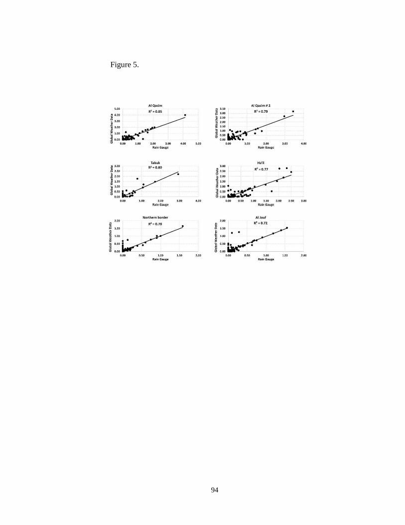
94
Figure 5.
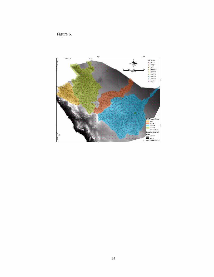
95
Figure 6.
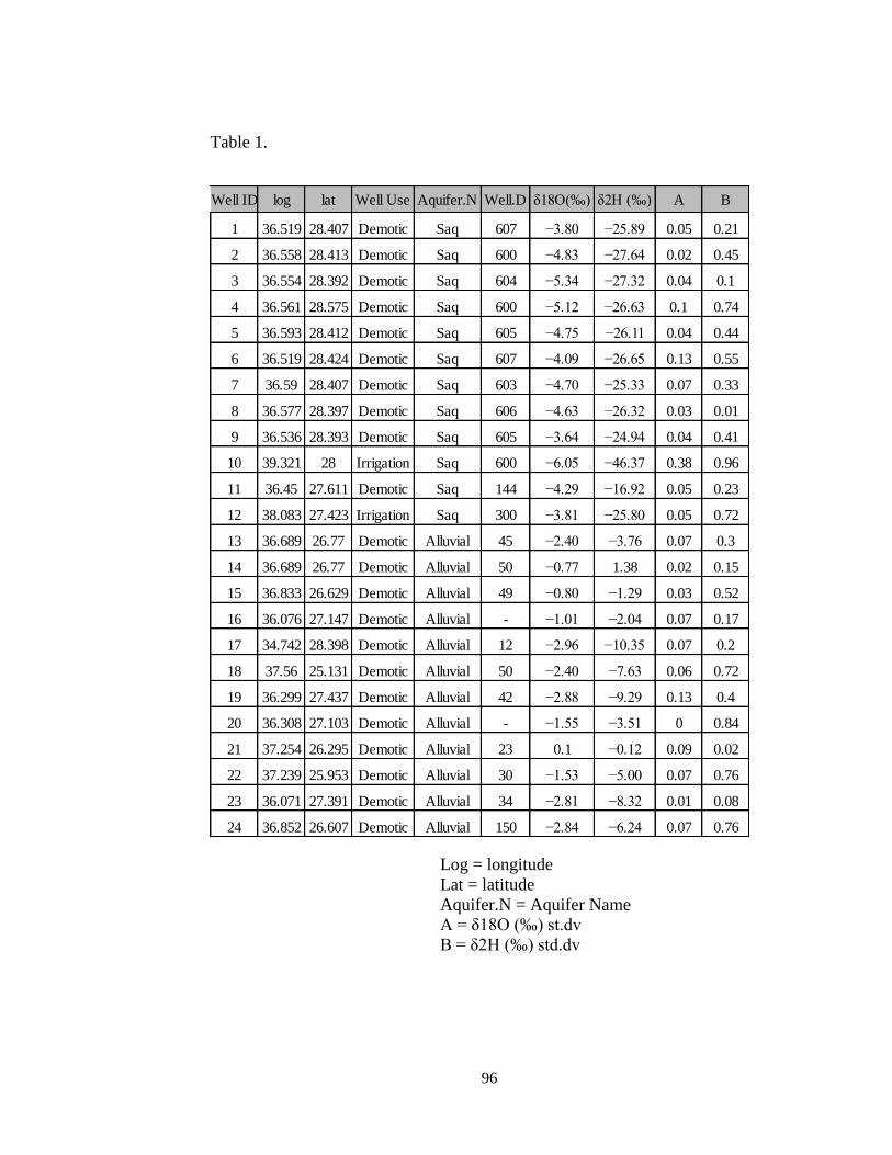
96
Table 1.
Log = longitude
Lat = latitude
Aquifer.N = Aquifer Name
A = δ18O (‰) st.dv
B = δ2H (‰) std.dv
Well ID log lat Well Use Aquifer.N Well.D δ18O(‰) δ2H (‰) A B
1 36.519 28.407 Demotic Saq 607 −3.80 −25.89 0.05 0.21
2 36.558 28.413 Demotic Saq 600 −4.83 −27.64 0.02 0.45
3 36.554 28.392 Demotic Saq 604 −5.34 −27.32 0.04 0.1
4 36.561 28.575 Demotic Saq 600 −5.12 −26.63 0.1 0.74
5 36.593 28.412 Demotic Saq 605 −4.75 −26.11 0.04 0.44
6 36.519 28.424 Demotic Saq 607 −4.09 −26.65 0.13 0.55
7 36.59 28.407 Demotic Saq 603 −4.70 −25.33 0.07 0.33
8 36.577 28.397 Demotic Saq 606 −4.63 −26.32 0.03 0.01
9 36.536 28.393 Demotic Saq 605 −3.64 −24.94 0.04 0.41
10 39.321 28 Irrigation Saq 600 −6.05 −46.37 0.38 0.96
11 36.45 27.611 Demotic Saq 144 −4.29 −16.92 0.05 0.23
12 38.083 27.423 Irrigation Saq 300 −3.81 −25.80 0.05 0.72
13 36.689 26.77 Demotic Alluvial 45 −2.40 −3.76 0.07 0.3
14 36.689 26.77 Demotic Alluvial 50 −0.77 1.38 0.02 0.15
15 36.833 26.629 Demotic Alluvial 49 −0.80 −1.29 0.03 0.52
16 36.076 27.147 Demotic Alluvial - −1.01 −2.04 0.07 0.17
17 34.742 28.398 Demotic Alluvial 12 −2.96 −10.35 0.07 0.2
18 37.56 25.131 Demotic Alluvial 50 −2.40 −7.63 0.06 0.72
19 36.299 27.437 Demotic Alluvial 42 −2.88 −9.29 0.13 0.4
20 36.308 27.103 Demotic Alluvial - −1.55 −3.51 0 0.84
21 37.254 26.295 Demotic Alluvial 23 0.1 −0.12 0.09 0.02
22 37.239 25.953 Demotic Alluvial 30 −1.53 −5.00 0.07 0.76
23 36.071 27.391 Demotic Alluvial 34 −2.81 −8.32 0.01 0.08
24 36.852 26.607 Demotic Alluvial 150 −2.84 −6.24 0.07 0.76
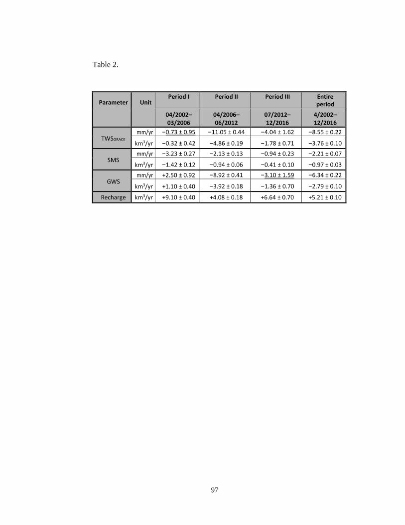
97
Table 2.
Parameter Unit Period I Period II Period III Entire
period
04/2002–03/2006
04/2006–06/2012
07/2012–12/2016
4/2002–12/2016
TWSGRACE mm/yr −0.73 ± 0.95 −11.05 ± 0.44 −4.04 ± 1.62 −8.55 ± 0.22
km3/yr −0.32 ± 0.42 −4.86 ± 0.19 −1.78 ± 0.71 −3.76 ± 0.10
SMS mm/yr −3.23 ± 0.27 −2.13 ± 0.13 −0.94 ± 0.23 −2.21 ± 0.07
km3/yr −1.42 ± 0.12 −0.94 ± 0.06 −0.41 ± 0.10 −0.97 ± 0.03
GWS mm/yr +2.50 ± 0.92 −8.92 ± 0.41 −3.10 ± 1.59 −6.34 ± 0.22
km3/yr +1.10 ± 0.40 −3.92 ± 0.18 −1.36 ± 0.70 −2.79 ± 0.10
Recharge km3/yr +9.10 ± 0.40 +4.08 ± 0.18 +6.64 ± 0.70 +5.21 ± 0.10
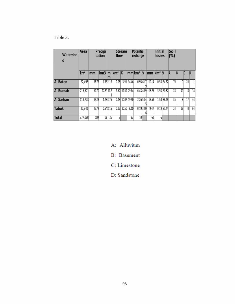
98
Table 3.
Watershed
Area Precipitation
Stream flow
Potential recharge
Initial losses
Soil (%)
km2 mm km3 mm
km3 % mm km3 % mm km3 % A B C D
Al Baten 27,496 55.77 1.53 2.18 0.06 3.91 34.46 0.95 61.79
19.14 0.53 34.32 79 0 20 1
Al Rumah 215,521 59.79 12.89 11.71
2.52 19.59 29.84 6.43 49.91
18.25 3.93 30.52 28 49 8 14
Al Sarhan 113,723 37.23 4.23 3.75 0.43 10.07 19.90 2.26 53.45
13.58 1.54 36.48 35 3 17 44
Tabuk 20,341 26.72 0.54 8.15 0.17 30.50 9.10 0.19 34.06
9.47 0.19 35.44 24 12 0 64
Total 377,080 180 19 26 3 93 10 60 6
99
Manuscript Ш
Groundwater Quality Patterns and Spatio-temporal
Change in the Depletion Regions of Arabian Shield and
Arabian Shelf: Implications of Public Health
Othman Abdurrahman Fallatah1, 2, Dawn Cardace1, Ali S
Akanda1
1) Department of Civil and Environmental Engineering, University of
Rhode Island, Kingston, RI 02881, USA
2) Faculty of Engineering, Radiation Protection & Training Centre,
King Abdul-Aziz University,
P.O. Box 80204, Jeddah 21589, Saudi Arabia
100
1. Abstract:
Groundwater quality is a critical issue in the arid and semi-arid
countries, where it is one of the most reliable sources on which
people depend. Water quality is a vital concern in the Kingdom of
Saudi Arabia (KSA) affecting as it affects the health of its people, the
growth of its agriculture, and its economic development. In this
study: the objectives were to (1) investigate the depletion rate of
Groundwater storage (GWS) in the studying area by using art of
Gravity Recovery and Climate Experiment (GRACE) solution during
(2002-2016); (2) determine the ionic composition of cations and
anions for 24 samples, 12 samples from Arabian Shield, and 12 from
Arabian Shelf in Saudi Arabia. (3) Assess the characterization of the
water quality of the aquifer by using Piper diagram. The results show
GRACE-derived GWS depletion (-2 ± 0.13 km 3/ year). The results
of ionic composition reveal two main groups (Group I: well depths:
144 m – 607 m; Group II: well depths: 12 m – 150 m). The de Group
I (Saq aquifer; fossil water), ionic composition results within limits
for all samples, compared to Group II (alluvial aquifer; mixed water).
The classification of groundwater was done by using Piper diagram,
where most of the samples in Arabian Shelf (85 %) falls in the type
of (Mix Ca-Mg-Cl-SO4). In the Arabian Shield, 50% of the samples
falls in the type of (Ca-Cl). Where most of the samples (98%) are
101
from domestic wells, and the people use it as drinking water, it is
essential to assess the radioactive analysis and the water quality for
those samples which is higher than Water Health Organization
(WHO) standard and understanding its impacts on public health.
KEYWORDS
Groundwater quality, Arabian Shield, Arabian Shelf, GRACE, Hydro
chemical, Cations, Anions
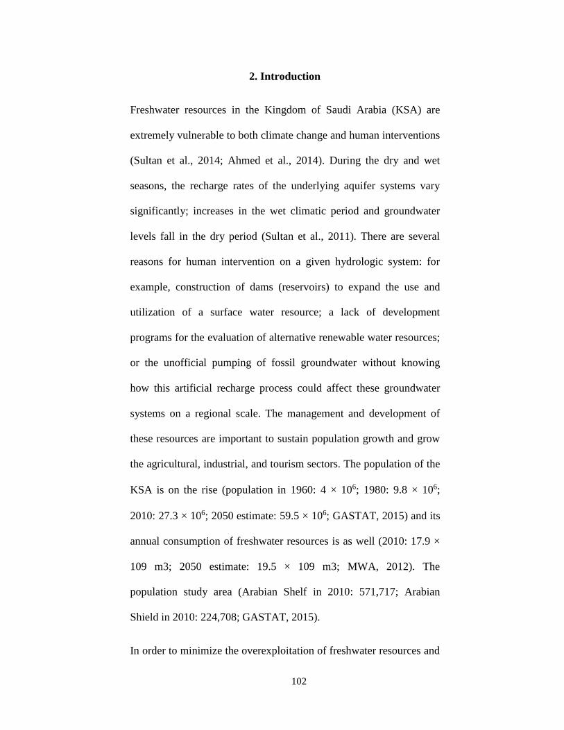
102
2. Introduction
Freshwater resources in the Kingdom of Saudi Arabia (KSA) are
extremely vulnerable to both climate change and human interventions
(Sultan et al., 2014; Ahmed et al., 2014). During the dry and wet
seasons, the recharge rates of the underlying aquifer systems vary
significantly; increases in the wet climatic period and groundwater
levels fall in the dry period (Sultan et al., 2011). There are several
reasons for human intervention on a given hydrologic system: for
example, construction of dams (reservoirs) to expand the use and
utilization of a surface water resource; a lack of development
programs for the evaluation of alternative renewable water resources;
or the unofficial pumping of fossil groundwater without knowing
how this artificial recharge process could affect these groundwater
systems on a regional scale. The management and development of
these resources are important to sustain population growth and grow
the agricultural, industrial, and tourism sectors. The population of the
KSA is on the rise (population in 1960: 4 × 10⁶; 1980: 9.8 × 10⁶;
2010: 27.3 × 10⁶; 2050 estimate: 59.5 × 10⁶; GASTAT, 2015) and its
annual consumption of freshwater resources is as well (2010: 17.9 ×
109 m3; 2050 estimate: 19.5 × 10⁹ m3; MWA, 2012). The
population study area (Arabian Shelf in 2010: 571,717; Arabian
Shield in 2010: 224,708; GASTAT, 2015).
In order to minimize the overexploitation of freshwater resources and
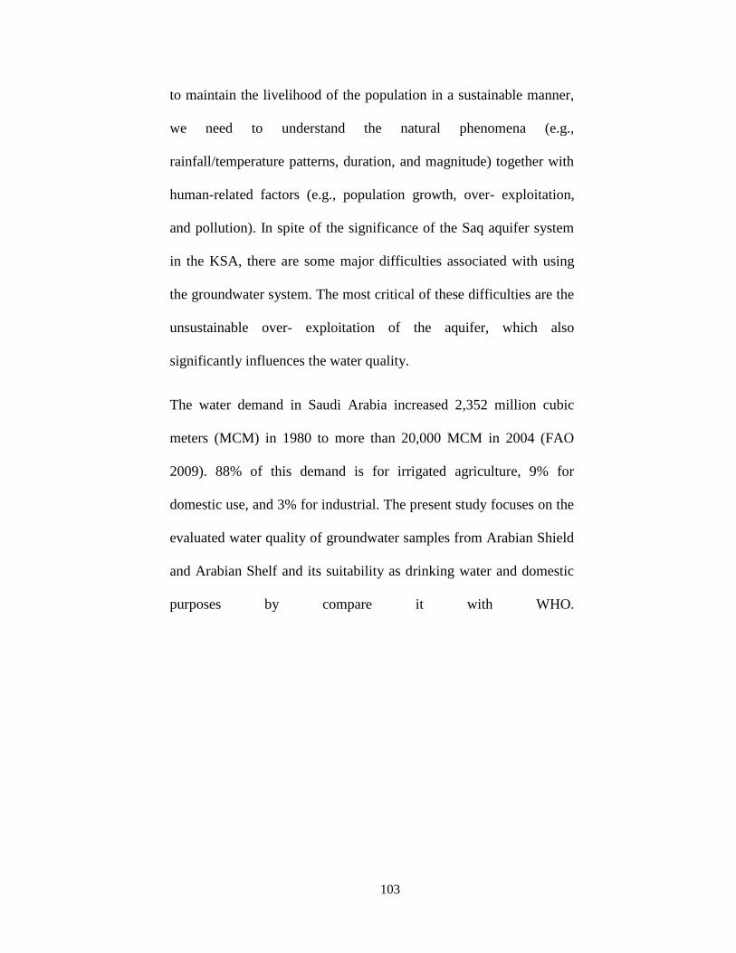
103
to maintain the livelihood of the population in a sustainable manner,
we need to understand the natural phenomena (e.g.,
rainfall/temperature patterns, duration, and magnitude) together with
human-related factors (e.g., population growth, over- exploitation,
and pollution). In spite of the significance of the Saq aquifer system
in the KSA, there are some major difficulties associated with using
the groundwater system. The most critical of these difficulties are the
unsustainable over- exploitation of the aquifer, which also
significantly influences the water quality.
The water demand in Saudi Arabia increased 2,352 million cubic
meters (MCM) in 1980 to more than 20,000 MCM in 2004 (FAO
2009). 88% of this demand is for irrigated agriculture, 9% for
domestic use, and 3% for industrial. The present study focuses on the
evaluated water quality of groundwater samples from Arabian Shield
and Arabian Shelf and its suitability as drinking water and domestic
purposes by compare it with WHO.
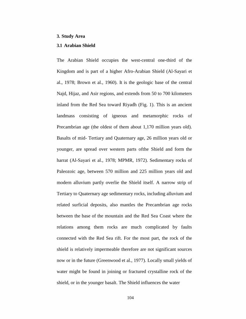
104
3. Study Area
3.1 Arabian Shield
The Arabian Shield occupies the west-central one-third of the
Kingdom and is part of a higher Afro-Arabian Shield (Al-Sayari et
al., 1978; Brown et al., 1960). It is the geologic base of the central
Najd, Hijaz, and Asir regions, and extends from 50 to 700 kilometers
inland from the Red Sea toward Riyadh (Fig. 1). This is an ancient
landmass consisting of igneous and metamorphic rocks of
Precambrian age (the oldest of them about 1,170 million years old).
Basalts of mid- Tertiary and Quaternary age, 26 million years old or
younger, are spread over western parts ofthe Shield and form the
harrat (Al-Sayari et al., 1978; MPMR, 1972). Sedimentary rocks of
Paleozoic age, between 570 million and 225 million years old and
modern alluvium partly overlie the Shield itself. A narrow strip of
Tertiary to Quaternary age sedimentary rocks, including alluvium and
related surficial deposits, also mantles the Precambrian age rocks
between the base of the mountain and the Red Sea Coast where the
relations among them rocks are much complicated by faults
connected with the Red Sea rift. For the most part, the rock of the
shield is relatively impermeable therefore are not significant sources
now or in the future (Greenwood et al., 1977). Locally small yields of
water might be found in joining or fractured crystalline rock of the
shield, or in the younger basalt. The Shield influences the water
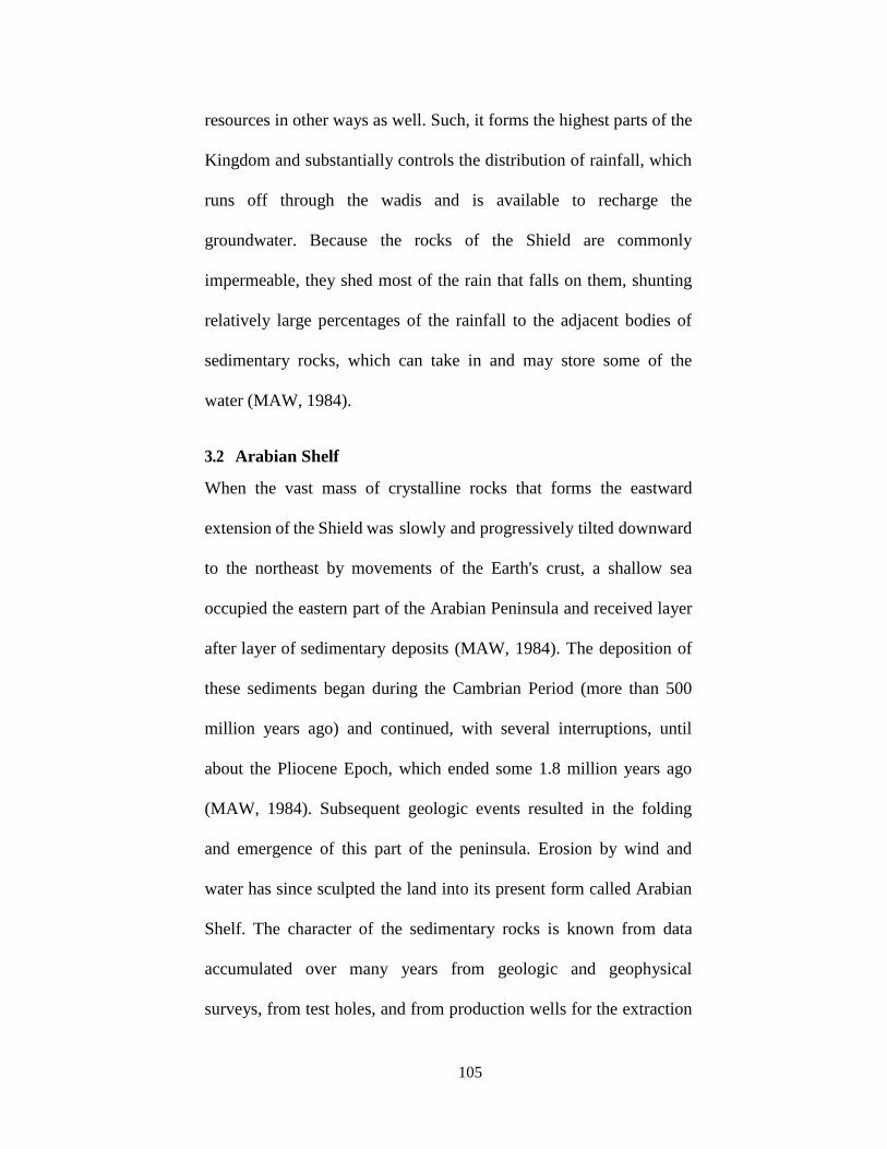
105
resources in other ways as well. Such, it forms the highest parts of the
Kingdom and substantially controls the distribution of rainfall, which
runs off through the wadis and is available to recharge the
groundwater. Because the rocks of the Shield are commonly
impermeable, they shed most of the rain that falls on them, shunting
relatively large percentages of the rainfall to the adjacent bodies of
sedimentary rocks, which can take in and may store some of the
water (MAW, 1984).
3.2 Arabian Shelf
When the vast mass of crystalline rocks that forms the eastward
extension of the Shield was slowly and progressively tilted downward
to the northeast by movements of the Earth's crust, a shallow sea
occupied the eastern part of the Arabian Peninsula and received layer
after layer of sedimentary deposits (MAW, 1984). The deposition of
these sediments began during the Cambrian Period (more than 500
million years ago) and continued, with several interruptions, until
about the Pliocene Epoch, which ended some 1.8 million years ago
(MAW, 1984). Subsequent geologic events resulted in the folding
and emergence of this part of the peninsula. Erosion by wind and
water has since sculpted the land into its present form called Arabian
Shelf. The character of the sedimentary rocks is known from data
accumulated over many years from geologic and geophysical
surveys, from test holes, and from production wells for the extraction
106
of petroleum, or water. The sedimentary rocks consist mainly of
limestone, sandstone, and shale. They have an aggregate
thickness as high as 5,500 meters, 1-5 thinning toward the west
as the basement rocks become shallower. The critical water
controlling role of the geological framework is seen in the fact
that this sequence of sedimentary rocks virtually all the naturally
occurring fresh water that is available in the kingdom
(Greenwood et al., 1977). Some of the sedimentary rock layers,
mainly sandstone and limestone, have considerable
interconnected pore space or other openings that are filled with
fresh water and, they are capable of transmitting the water
readily to wells (Al-Sayari et al., 1978; Brown et al., 1960;
Greenwood et al., 1977; MPMR, 1972; Brown et al., 1978;
MacDonald et al., 1975).
4. Data and Methods:
4.1 Groundwater depletion from GRACE
GRACE is a joint between National Aeronautics and Space
Administration (NASA) and the German Aerospace Center (DLR)
mission that was launched in March 2002 to map the Earth’s static
and temporal global gravity fields (Tapley et al. 2004). The
variability in Earth’s gravity field is directly related to the
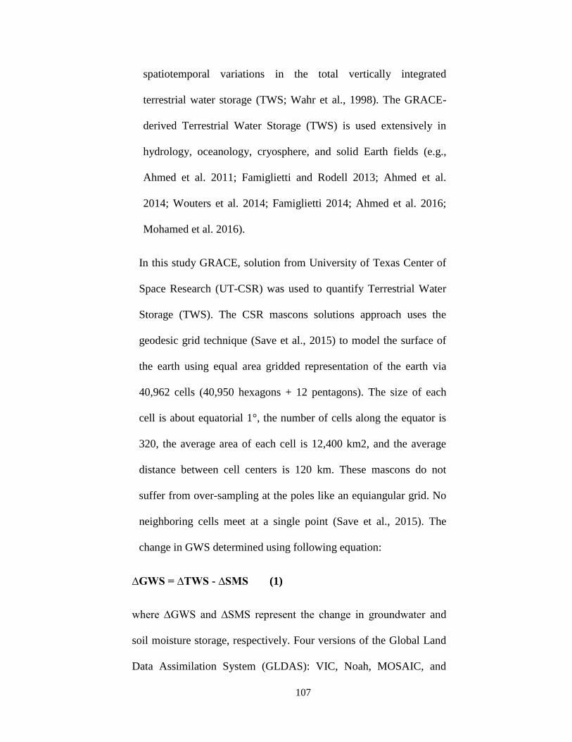
107
spatiotemporal variations in the total vertically integrated
terrestrial water storage (TWS; Wahr et al., 1998). The GRACE-
derived Terrestrial Water Storage (TWS) is used extensively in
hydrology, oceanology, cryosphere, and solid Earth fields (e.g.,
Ahmed et al. 2011; Famiglietti and Rodell 2013; Ahmed et al.
2014; Wouters et al. 2014; Famiglietti 2014; Ahmed et al. 2016;
Mohamed et al. 2016).
In this study GRACE, solution from University of Texas Center of
Space Research (UT-CSR) was used to quantify Terrestrial Water
Storage (TWS). The CSR mascons solutions approach uses the
geodesic grid technique (Save et al., 2015) to model the surface of
the earth using equal area gridded representation of the earth via
40,962 cells (40,950 hexagons + 12 pentagons). The size of each
cell is about equatorial 1°, the number of cells along the equator is
320, the average area of each cell is 12,400 km2, and the average
distance between cell centers is 120 km. These mascons do not
suffer from over-sampling at the poles like an equiangular grid. No
neighboring cells meet at a single point (Save et al., 2015). The
change in GWS determined using following equation:
∆GWS = ∆TWS - ∆SMS (1)
where ∆GWS and ∆SMS represent the change in groundwater and
soil moisture storage, respectively. Four versions of the Global Land
Data Assimilation System (GLDAS): VIC, Noah, MOSAIC, and
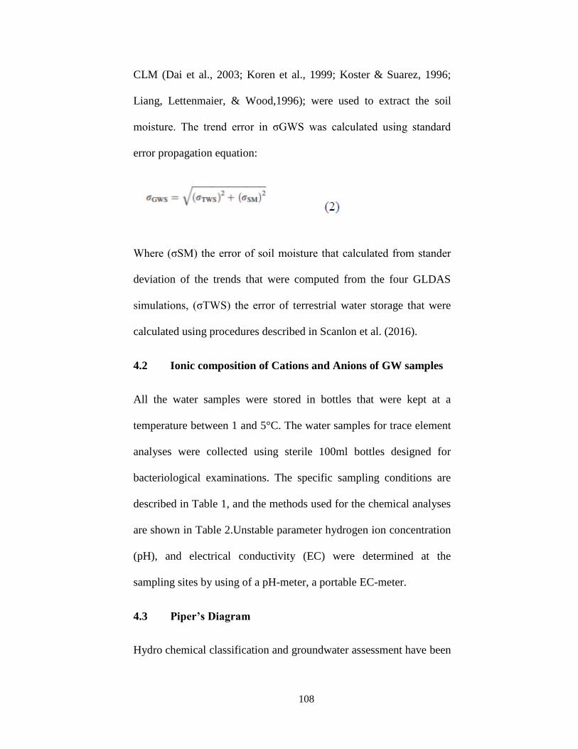
108
CLM (Dai et al., 2003; Koren et al., 1999; Koster & Suarez, 1996;
Liang, Lettenmaier, & Wood,1996); were used to extract the soil
moisture. The trend error in σGWS was calculated using standard
error propagation equation:
Where (σSM) the error of soil moisture that calculated from stander
deviation of the trends that were computed from the four GLDAS
simulations, (σTWS) the error of terrestrial water storage that were
calculated using procedures described in Scanlon et al. (2016).
4.2 Ionic composition of Cations and Anions of GW samples
All the water samples were stored in bottles that were kept at a
temperature between 1 and 5°C. The water samples for trace element
analyses were collected using sterile 100ml bottles designed for
bacteriological examinations. The specific sampling conditions are
described in Table 1, and the methods used for the chemical analyses
are shown in Table 2.Unstable parameter hydrogen ion concentration
(pH), and electrical conductivity (EC) were determined at the
sampling sites by using of a pH-meter, a portable EC-meter.
4.3 Piper’s Diagram
Hydro chemical classification and groundwater assessment have been
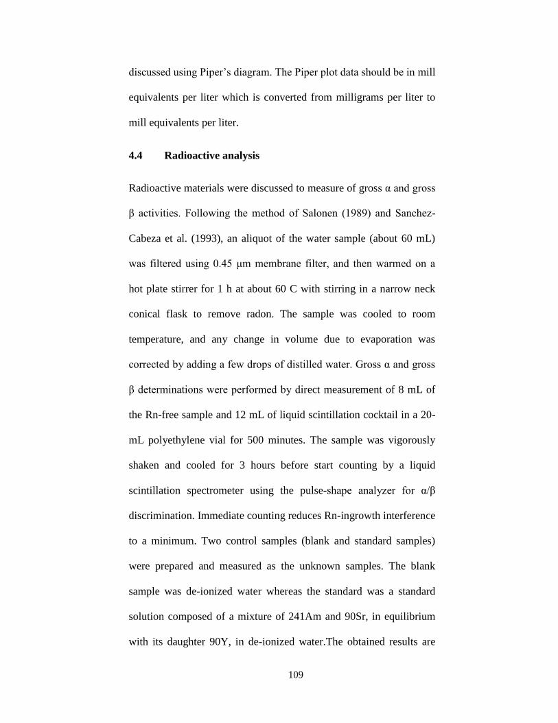
109
discussed using Piper’s diagram. The Piper plot data should be in mill
equivalents per liter which is converted from milligrams per liter to
mill equivalents per liter.
4.4 Radioactive analysis
Radioactive materials were discussed to measure of gross α and gross
β activities. Following the method of Salonen (1989) and Sanchez-
Cabeza et al. (1993), an aliquot of the water sample (about 60 mL)
was filtered using 0.45 μm membrane filter, and then warmed on a
hot plate stirrer for 1 h at about 60 C with stirring in a narrow neck
conical flask to remove radon. The sample was cooled to room
temperature, and any change in volume due to evaporation was
corrected by adding a few drops of distilled water. Gross α and gross
β determinations were performed by direct measurement of 8 mL of
the Rn-free sample and 12 mL of liquid scintillation cocktail in a 20-
mL polyethylene vial for 500 minutes. The sample was vigorously
shaken and cooled for 3 hours before start counting by a liquid
scintillation spectrometer using the pulse-shape analyzer for α/β
discrimination. Immediate counting reduces Rn-ingrowth interference
to a minimum. Two control samples (blank and standard samples)
were prepared and measured as the unknown samples. The blank
sample was de-ionized water whereas the standard was a standard
solution composed of a mixture of 241Am and 90Sr, in equilibrium
with its daughter 90Y, in de-ionized water.The obtained results are
110
compared to the World Health Organization (WHO) guidance levels,
to show a preliminary assessment of the radiological risk attached to
groundwater use.
5. Results
5.1 GWS from GRACE
The observed GRACE-derived TWS depletions over the study area
are related to variations in both soil moisture storage and GWS since
GRACE has no vertical resolution. To quantify the GRACE-derived
GWS variations over the Saq aquifer system, the GLDAS-derived
soil moisture estimates are subtracted from the GRACE-derived TWS
averaged from UT-CSR mascons equation (1). Figure 4 shows the
temporal variations in the GRACE-derived groundwater estimates
over the Saq aquifer. Examination of (Figure 4) reveals a
groundwater depletion rate of−2.11 ± 0.13 km3/yr.
5.2 TDS
Table 3 shows the summary of the ionic composition in Arabian shelf
and Arabian shield. The water samples are somewhat acidic to
neutral with PH values ranging 6.40 to 7.80 in Arabian Shelf, and
from 7.10 to 8 in the Arabian Shield. Electrical conductivity (EC)
ranges from 460 to 1100 μS/cm, with an average of 766.64 μS/cm in
Arabian Shelf. On the other side, 95% of the samples are crossing the
maximum permissible limit of EC (1,500 μS/cm) in the Arabian
111
Shield. The total dissolved solids (TDS) were measured through
summing up all major ions concentrations, which range from 253 to
660 mg/l in Arabian Shelf with an average value of 479.92 mg/l.
Only 20 % of the samples have TDS value <500 mg/l, which is
below the stander 1200 mg/l from WHO. The water samples from
Arabian Shield has high TDS, which is the max 5417.5 mg/l, and the
minimum 942.7 mg/l around 95% of the samples is exceeding the
permeation limit in water use. These high TDS values are probably
linked to a local source of contamination of the aquifer, such as
inadequate well completion and leading to pollution from the soil
surface into the considered well through non-cemented or poorly
cemented annular space (MWA, 2012). TDS distribution shows that
the highest values, i.e., from 1,200 to 5,000 mg/l, are observed in
areas where the geological formations contain aquifers outcrops. The
TDS in deeper groundwater samples is generally below 1,200 mg/l,
and in some places less than 500 mg/l. (MWA, 2012).
5.3 Ionic composition of Arabian Shelf and Arabian Sheild
Investigation focused on cations and anions distributions of Na+,
Ca++, Mg++, K+ and Cl−, SO4−2, HCO3, NO3 respectively.
Investigation Table.3 shows most of the cations and anions in
Arabian Shield are exceeding the stander of WHO due several
reasons that affect the water quality in that region such high
evaporation, high abstraction which is affect the gradients of the
112
aquifer, and industrial activities. On other side, the ionic composition
of Arabian Shelf are within the stander of WHO, but the radioactive
materials of gross alpha and beta are exceeding WHO’s guidance
level.
5.4 Hydrochemical classification
The classification of groundwater analysis was done using Piper’s
diagram (Piper 1944). The ternary diagrams (Fig. 4) are showed three
types of groundwater signed in this study, type (І) in the confined
section near to the outcrops all over the study area, type (ІІ) in the
basaltic area, in the confined section, and to the north of the east part,
and type (Ш) in the outcrops and shallow wells in the west part of the
study area and in some deep wells near the outcrops in the east part.
Most of the samples falls in-group І and ІІ, which show evolved (Ca-
Cl) and (Mix Ca-Mg-Cl- SO4) type where unique chemical masking
is achieved through rock-water interaction, ion exchange, and reverse
ion exchange; reactions within unsaturated zones; increased resident
time; and anthropogenic influences. The group III water type (Ca-
HCO3) representing meteoric signatures or fresh recharged water
constitutes only 5 % of the total samples.
5.5 Comparison of groundwater quality in the depletion
regions between 2006 and 2016
As part of the investigation, we also compared groundwater quality in
113
the depletion regions between groundwater quality data in 2006 that
was provided by MEWA and in 2016 tested in our lab from water
samples directly collected from the area (Fig. 2). The statistical
distributions in the Arabian Shelf of TDS are very similar, and no
significant changes are identified between 2006 and 2016 (Fig. 3).
However, in Arabian Shield samples, there is a significant increase of
TDS in 2016, and that might be related to reverse pumping the
hydraulic gradients resulting increasing dissolved mineral
concentration especially in the coastal aquifers. Therefore most of the
samples located on Arabian Shield have high ionic composition
above drinking water standards (MWA, 2012)
5.6 Radio analysis results
We also performed radiological analysis of the Saq aquifer system
and adjoining waters to investigate links with groundwater patterns
and radioactive quality. Twelve wells samples are located in
basement granite, and related alluvium, along with the edge; and
other 12 wells samples are located in the unconfined sector of the Saq
aquifer. The results showed most of the samples that located in Saq
aquifer area have a high value of Gross α and Gross β exceeding
WHO limit (Table 3). The basement is located below the Saq aquifer
and laterally limits its extension westwards. The Saq aquifer is
overlain by Hanadir shale. The radiological activity of the different
rock types as mentioned in literature (Alabdula’aly, 1999; Iyengar et
114
al., 1990; Michel, 1991; Molinari et al., 1990; Aoudeh, 1994 ) are
summarized as follows:
- Granite basement with an average content of 3 mg/kg of
uranium: 1-190 Bq/kg of Ra-226.
- Sandstones are not known for their high radionuclide
concentration: about 1 mg/kg of uranium and activity of less than 60
Bq/kg of Ra-226.
- Shale with an average content of 3.7 mg/kg of uranium: 10-
2,300 Bq/kg of Ra-226.
Therefore, the origin of radioactivity in the Saq aquifer water seems
more likely related to adjacent layers.
6. Conclusion
The quality of groundwater in the Kingdom of Saudi Arabia plays a
significant role in maintaining the health of people, which is the most
critical source of drinking water in the Kingdom. Therefore, it is
imperative to monitor groundwater quality continuously and make
sure that it meets the stander of drinking water is necessary for the
safety and health of the people.
This study focused on examining the quality of water in two regions
with different geological characteristics, and we found the difference
in water quality used in those regions. Most of the samples collected
115
from the Arabian Shield, from wells used for domestic and drinking
purposes, show that the percentage of TDS is very high and above the
limit allowed globally. According to the WHO, this water is not
suitable for drinking but can be used for others purposes; the high
proportion of salinity in this water related to saltwater encroachment
occur in coastal aquifers where pumping reverses the hydraulic
gradients resulting in increasing dissolved mineral concentrations.
Because of that, most of the cations and anions in the samples have a
high concentration, above the standard limit for drinking water. The
water type for this region was tested by using Piper diagram to
explain the characterization of water quality; most of the water were
related to (Ca-Cl) and (Mix Ca-Mg-Cl-SO4) which is the samples are
in the confined section near to the outcrops all over the study area,
and other falls in the water type of (Ca-HCO3) representing
recharged water.
The results of the radioactive analysis in this region were average and
within the standard limits for drinking water.
The samples collected from Arabian Shelf have a good quality of
ionic compositions of cations and anions and within the standard
limit of drinking water. Piper diagram shows the majority of samples
in Arabian Shelf falls in the type of (Mix Ca-Mg-Cl-SO4) and show
evolved groundwater type that related to the different periods of
climate conditions. Our investigation in this region for radioactive
116
analysis revealed most of the samples that located in Saq aquifer area
have a high value of Gross α and Gross β exceeding the WHO limit.
According to WHO, there is no health concern for using these
samples from both regions in the short term. These study findings are
being shared with decision makers in relevant governmental agencies
and decision makers to manage and develop groundwater quality in
these regions.
7. Acknowledgments
The authors would like to sincerely thank the Ministry of Water and
Environment Tabuk branch for their efforts to analyze the water
quality of the samples that was used in this project. Also great thanks
to King Abdulaziz University for their help and advice on
radiochemical analysis.
117
8. References
1. Ahmed, M., Sultan M., Wahr, J., Yan, E., Milewski, A.,
Sauck, W., Welton, B. (2011).
Integration of GRACE (Gravity Recovery and Climate
Experiment) data with traditional data sets for a better
understanding of the time‐ dependent water partitioning in
African watersheds. (5): 479–482.
https://doi.org/10.1130/G31812.1
2. Ahmed, M., Sultan, M., Wahr, J., & Yan, E. (2014). The use
of GRACE data to monitor natural and anthropogenic induced
variations in water availability across Africa. Earth‐ Science
Reviews, 136, 289–300.
https://doi.org/10.1016/j.earscirev.2014.05.009
3. Ahmed, M., Sultan, M., Yan, E., & Wahr, J. (2016).
Assessing and improving land surface model outputs over
Africa using GRACE, field, and remote sensing data. Surveys
in Geophysics, 37(3), 529–556. https://doi.org/
10.1007/s10712‐016‐9360‐8
4. Al-Sayari, S.S., and Zotl, J.G., eds., 1978, Quaternary Period
in Saudi Arabia: Wien- New York, Springer-Verlag, 334 p.
5. Alabdula’aly, A. I. (1999). Occurrence of radon in the central
region groundwater of Saudi Arabia. Journal of environmental
radioactivity, 44(1), 85-95. ISO 690
118
6. Aoudeh S.M. and Al-Hajri S.A. (1994). Regional distribution
and chronostratigraphy of the Qusaiba Member of the Qalibah
Formation in the Nafud Basin, northwestern Saudi Arabia.
Geo ’94, The Middle East Petroleum Geosciences. Vol. 1. pp
143-154. April 25- 27, 1994, Bahrain. Edited by M.I. Al-
Husseini, published by GulfPetrolLink, Bahrain.
7. Brown, G.F., 1960, Geomorphology of Western and Central
Saudi Arabia: International Geological Congress, 21st,
Copenhagen, 1960, Proceedings, sec. 9, p. 150-159.
8. Brown, G.F., and Jackson, R.O., 1978, an Overview of the
Geology of Western Arabia: U.S. Geological Survey, Saudi
Arabian Project Report 250, 23 p.
9. F. Schonhofer, K. Pock, H. Friedmann, “Radon surveys with
charcoal and liquid scintillation counting,” J. Radioanal. Nucl.
Chem. Articles, 193, 337-346 (1995).
10. Famiglietti, J. S. (2014). The global groundwater crisis.
Nature Climate Change, 4(11), 945–948.
https://doi.org/10.1038/nclimate2425
11. Famiglietti, J. S., & Rodell, M. (2013). Water in the balance.
Science, 340, 1300–
1301.https://doi.org/10.1126/science.1236460
12. Greenwood, W.R., Anderson, R.E., Fleck, R.S., and Roberts
119
R. S., 1977, Precambrian Geologic History and Plate Tectonic
Evolution of the Arabian Shield: U.S. Geological Survey,
Saudi Arabian Project Report 222, 97 p.
13. GASTAT. (2016). General authority for statistics Available at
http://www. stats.gov.sa/en [Accessed 24 December 2016]
14. Iyengar, M. A. R. (1990). The natural distribution of radium.
The environmental behavior of radium, 1, 59-128.
15. MacDonald, M., and Partners, 1975, Final Report V.,
Regional Geology and Geophysical Investigation: Ministry of
Agriculture and Water, Riyadh, Saudi Arabia, no. 18, p. 70-
73.
16. (MAW) Ministry of Agriculture and Water (1984). Water
Atlas of Sandi Arabia. 112 pp.
17. MEWA. (2016). Ministry of environment, water, and
agriculture Available at
http://www.mowe.gov.sa/enindex.aspx?AspxAutoDetectCook
ie Support=1
18. (MPMR) Ministry of Petroleum and Mineral Resources
(1972), Tectonic Map of the Arabian Peninsula: Saudi
Arabian Deputy Ministry for Mineral Resources, Ministry of
Petroleum and Mineral Resources, Arabian Peninsula Map
AP-2, scale
19. Michel, J. (1991). Relationship of radium and radon with
120
geological formations. In: “Radon, Radium, and Uranium in
drinking water,” eds. Richard Cothern C. and Rebers P.A.
20. Mohamed, A., Sultan, M., Ahmed, M., Yan, E., & Ahmed, E.
(2016). Aquifer recharge, depletion, and connectivity:
Inferences from GRACE, land surface models, geochemical,
and geophysical data. GSA Bullitin, 1–13.
https://doi.org/10.1130/B31460.1
21. Molinari J., and Snodgrass W.J. (1990). The chemistry and
radiochemistry of radium and the other elements of the
uranium natural decay series, in: “The environmental
behavior of radium,” Vol.1, IAEA.
22. Piper, A. M. (1944). A graphical procedure in the
geochemical interpretation of water analyses, transactions.
American Geophysical Union, 25, 914–928.
23. S. Chalupnik, J.M. Lebecka, “Determination of 226Ra, 228Ra
and 224Ra in water and aqueous solutions by liquid
scintillation counting”, “Liquid scintillation spectrometry
1992”, Edited by J.E. Noakes, F. Schonhofer and H.A.
Polach, RADIOCARBON 1993, pp. 397-403.
24. Scanlon BR, Zhang Z, Save H et al. (2016) Global evaluation
of new GRACE mascon products for hydrologic applications.
Water Resour Res 52:9412–9429
25. Save, H., Bettadpur, S., & Tapley, B. (2016). High-resolution
121
CSR GRACE RL05 mascons. Journal of Geophysical
Research.
26. Schmidt, D.L., Hadley, D.G., Greenwood, W.R., Gonzalez,
Lewis, Coleman, R.G., and Brown, G.F., 1972, Stratigraphy
and Tectonism of the Southern Part of the Precambrian Shield
of Saudi Arabia: U.S. Geological Survey, Saudi Arabian
Project Report 139, 36 p.
27. Sharaf, M. A., & Hussein, M. T. (1996). Groundwater quality
in the Saq aquifer, Saudi Arabia. Hydrological sciences
journal, 41(5), 683-696.
28. Sultan, M., Metwally, S., Milewski, A.,…Welton, B. (2011).
Modern recharge to fossil aquifers: Geochemical,
geophysical, and modeling constraints. Journal of Hydrology
403, 14–24. doi: 10.1016/j.jhydrol.2011.03.036
29. Sultan, M., Ahmed, M., Wahr, J., Yan, E., & Emil, M. K.
(2014). Monitoring aquifer depletion from space: Case studies
from the Saharan and Arabian aquifers. In V. Lakshmi (Ed.),
AGU Geophysical Monograph # 206. Remote sensing of the
terrestrial water cycle (pp. 349–366).
30. Wahr, J., Molenaar, M., & Bryan, F. (1998). Time variability
of the Earth's gravity field: Hydrological and oceanic effects
and their possible detection using GRACE. Journal of
Geophysical Research, 103(B12), 30205–30229.
122
31. Wouters, B., Bonin, J. A., Chambers, D. P., Riva, R. E. M.,
Sasgen, I., & Wahr J. (2014). GRACE, time‐varying gravity,
Earth system dynamics and climate change. Reports on
Progress in Physics 116801.
https://doi.org/10.1088/0034‐4885/77/11/116801
123
Figure Legends:
Fig. 1 Geological map for Arabian Shield and Arabian
Shelf.
Fig. 2 the differences in TDS between 2006 and 2016,
showed clearly the change in TDS of the samples those
located in the Arabian shield
Fig.3 Secular trend in Gravity Recovery and Climate
Experiment derived groundwater storage estimates
generated over the Arabian Peninsula from April 2002 to
April 2016, and samples locations
Fig.4 Piper diagram: Arabian Shelf and Arabian Shield
124
Table captions:
Table. 1 Preservation conditions of water samples
Table. 2 Analytical methods
Table. 3 Summaries results of water quality data in
Arabian Shelf and Arabian Shield
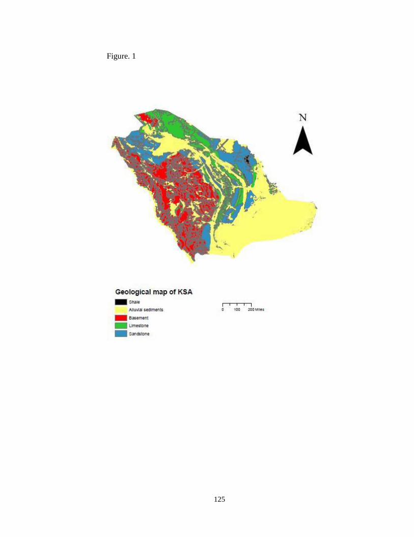
125
Figure. 1
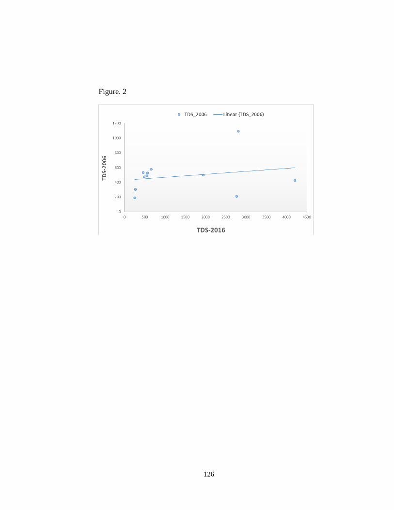
126
Figure. 2
TDS-
20
06
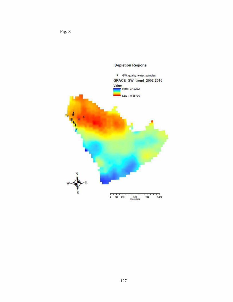
127
Fig. 3
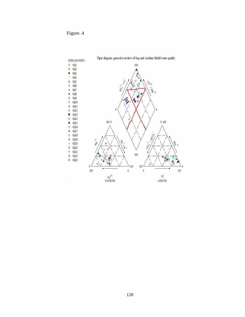
128
Figure. 4
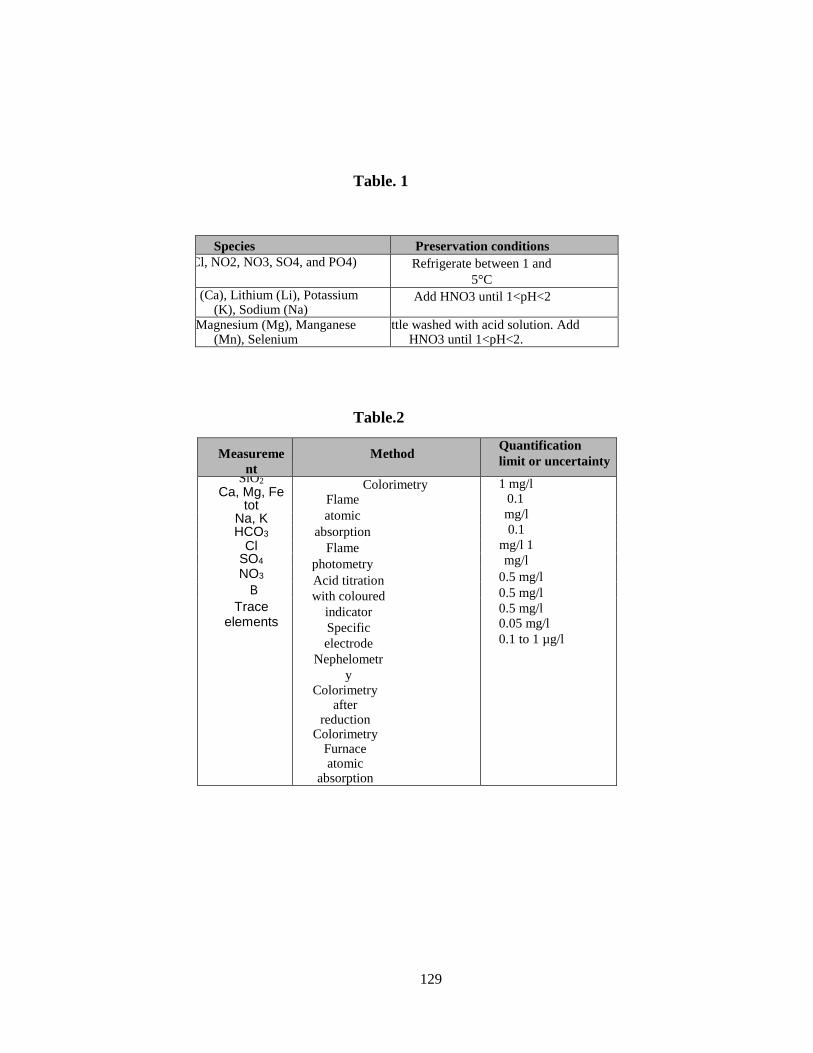
129
Table. 1
Species Preservation conditions
Anions (Br, F, Cl, NO2, NO3, SO4, and PO4) Refrigerate between 1 and
5°C
Calcium (Ca), Lithium (Li), Potassium (K), Sodium (Na)
Add HNO3 until 1<pH<2
Iron (Fe), Magnesium (Mg), Manganese (Mn), Selenium
Plastic bottle washed with acid solution. Add HNO3 until 1<pH<2.
Table.2
Measureme
nt
Method Quantification
limit or uncertainty
SiO2 Colorimetry Flame
atomic
absorption
Flame
photometry
Acid titration
with coloured
indicator
Specific
electrode
Nephelometr
y
Colorimetry after
reduction Colorimetry
Furnace atomic
absorption
1 mg/l 0.1
mg/l
0.1
mg/l 1
mg/l
0.5 mg/l
0.5 mg/l
0.5 mg/l 0.05 mg/l
0.1 to 1 µg/l
Ca, Mg, Fe tot
Na, K HCO3
Cl SO4 NO3
B
Trace elements
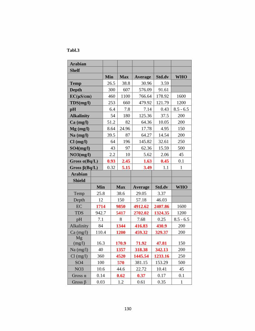
130
Tabl.3
Arabian
Shelf
Min Max Average Std.dv WHO
Temp 26.5 38.8 30.96 3.59
Depth 300 607 576.09 91.61
EC(μS/cm) 460 1100 766.64 178.92 1600
TDS(mg/l) 253 660 479.92 121.79 1200
pH 6.4 7.8 7.14 0.43 8.5 - 6.5
Alkalinity 54 180 125.36 37.5 200
Ca (mg/l) 51.2 82 64.36 10.05 200
Mg (mg/l) 8.64 24.96 17.78 4.95 150
Na (mg/l) 39.5 87 64.27 14.54 200
Cl (mg/l) 64 196 145.82 32.61 250
SO4(mg/l) 43 97 62.36 15.59 500
NO3(mg/l) 2.2 10 5.62 2.06 45
Gross α(Bq/L) 0.93 2.45 1.63 0.45 0.1
Gross β(Bq/L) 0.32 5.15 3.49 1.1 1
Arabian
Shield
Min Max Average Std.dv WHO
Temp 25.8 38.6 29.05 3.37
Depth 12 150 57.18 46.03
EC 1714 9850 4912.62 2407.86 1600
TDS 942.7 5417 2702.02 1324.35 1200
pH 7.1 8 7.68 0.25 8.5 - 6.5
Alkalinity 84 1344 416.83 430.9 200
Ca (mg/l) 110.4 1200 459.32 329.37 200
Mg
(mg/l) 16.3 170.9 71.92 47.81 150
Na (mg/l) 40 1357 318.38 342.13 200
Cl (mg/l) 360 4520 1445.54 1233.16 250
SO4 100 570 381.15 153.29 500
NO3 10.6 44.6 22.72 10.41 45
Gross α 0.14 0.62 0.37 0.17 0.1
Gross β 0.03 1.2 0.61 0.35 1
131
In conclusion
Groundwater monitoring includes both groundwater quantity (e.g.,
groundwater level and recharge rates) and quality monitoring (analysis
of selected physical and chemical variables). The purposes of
groundwater monitoring are to manage and develop the policy of the
groundwater resources and to predict the groundwater quality and
quantity due to natural processes and human impacts in time and
space. Therefore, in this situation we need to have a useful database
for assessment of the current state, anticipating changes and
forecasting trends in the future. My results in this dissertation will
contribute to the effective and efficient utilization of the Saq aquifer
water resources and will be used to promote the sustainable
development of the Arabian Peninsula and Middle East’s natural
resources in general. The findings have been and will be shared with
stakeholders and decision makers in relevant governmental agencies to
develop viable management scenarios for the water resources of the
Saq aquifer.
Future work
Mentoring groundwater quality and quantity characteristics on other
main and secondary aquifers in AP along with water usage,
demand, and demographics data.
To incorporate new data from GRACE-FO satellite, land surface
model, and rainfall data linked with water level data from the
distribution wells temporal variations of groundwater.

132
Development groundwater resources to support socio economic,
agricultural and industrial developments.
133
APPENDIX A
Gravity Recovery and Climate
Experiment (GRACE) Introduction
134
GRACE Mission:
1.1 Earth’s Gravity Field:
The Earth's gravity field is a product of its mass distribution. The
mass included deep within the Earth, at the surface of the Earth and
above the Earth's surface. That mass distribution is continually
changing. Examples include, but not limited to: (1) tides in the ocean
and solid Earth cause large mass variations at 12-hour and 24-hour
periods, (2) atmospheric disturbances associated with synoptic storms
or seasonal climatic differences may lead to variations in the
distribution of mass in the atmosphere, the ocean, and the water
stored on land, (3) mantle convection causes mass (Wahr, 2002).
The temporal variations in the mass distribution are responsible for
the variations in the Earth's gravity field with time. The time-variable
gravity field is successfully measured using either ground-based
instrumentation or satellites. These measurements could be used to
study a wide variety of geophysical processes that involve changes in
mass (Dickey et al., 1997). Most of the time variable signal comes
from the oceans, the atmosphere, the polar ice sheets, and the
variations storage of water and snow on land.
1.2 Time-Variable Gravity Field:
The gravity signals detected from the satellite are due entirely to the
underlying mass distribution. Until the launch of CHAMP

135
(Challenging Microsatellite Payload) in 2001 satellite time-variable
gravity solutions were based entirely on Satellite Laser Ranging
(SLR) observations. The most useful SLR measurements have
involved LAGEOS (launched by NASA
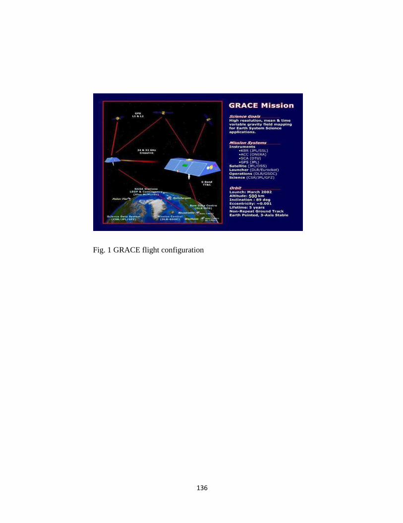
136
Fig. 1 GRACE flight configuration
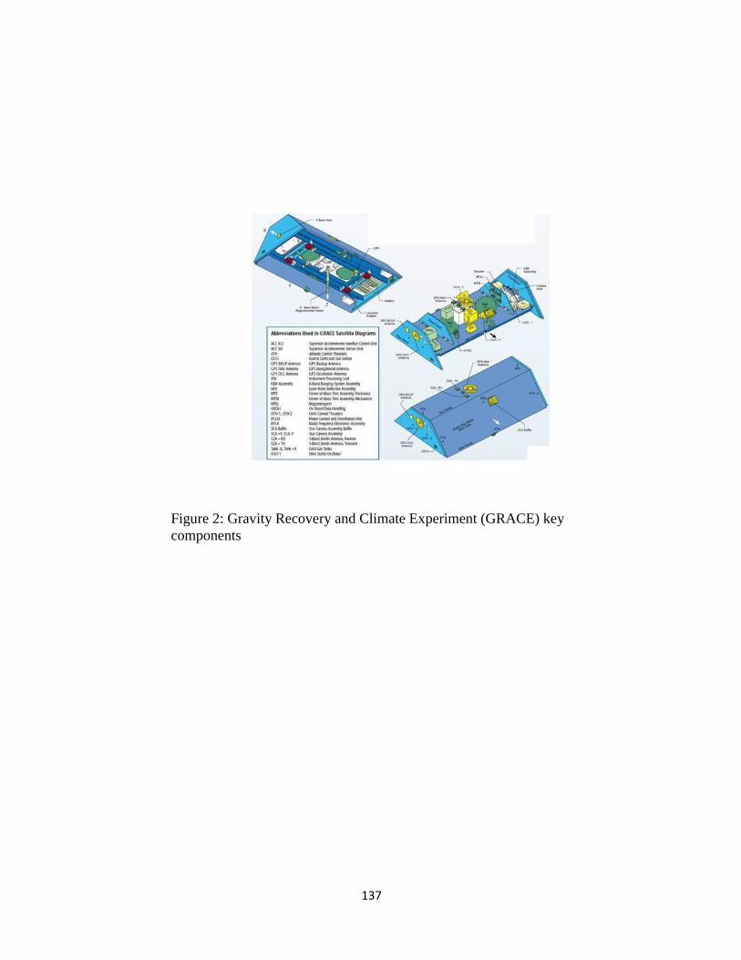
137
Figure 2: Gravity Recovery and Climate Experiment (GRACE) key
components
138
1.3 GRACE Instrumentation:
The critical components of the GRACE twin satellites (Fig. 2) are
listed below:
1- K-Band Ranging (KBR) system: Provides precise (up to 1
micrometer) measurements of the distance change between the two
satellites.
2- Accelerometer: Measures the non-gravitational forces on the
two satellites. 3- Star Camera: Provides the attitude of the
spacecraft.
4- GPS Receivers: Provide continues measurements regarding
satellites position, orbit determination, timing, and atmospheric
contributions.
1.4 GRACE Mission:
The GRACE mission consists of twin (GRACE A and GRACE B)
satellites flying in a polar orbit with an inclination of 89.5° and
altitude of 500 km (at launch) and approximately 200 km apart from
each other (Fig.1). The satellite altitude decays naturally (~30 m/day)
so that the ground track does not have a fixed repeat pattern (Tapley
et al., 2004b). The two satellites follow the same path and are
interconnected by a K-band (frequency: 12 to 63 GHz) microwave
link (Bettadpur, 2006; Flechtner, 2005). The orbits of the two
spacecraft are affected differently due to the spatial and temporal
139
variations in the Earth's gravity field, which can increase or decrease
the distance between them. These distance variations affect the
traveling time of the microwave signals, which are continually being
transmitted and received between satellites. The accuracy of the
measured separation distance is as small as 1 micron, about one over
100th the thickness of a human hair. When approaching an area of
higher gravity/mass, the front satellite, GRACE A, speeds up and
then slows down when flying above it. The second satellite, GRACE
B, on the trail of GRACE A will have the same fate. The GRACE
mission concept is summarized in Figure 3.
The disadvantage of having such a low (500 km) altitude is that
GRACE experiences greater atmospheric drag, which can cause
significant and unpredictable changes in the inter-satellite range
distance(Wahr, 2002). Each GRACE satellite has an onboard
accelerometer to measure non-gravitational accelerations. Those
measurements are transmitted to the ground where they are used to
correct the inter-satellite distance measurements (Wahr, 2002). Each
spacecraft also has an onboard GPS receiver, used to determine the
orbital motion of each spacecraft in the global GPS reference frame
and to improve the gravity field solutions at global-scale wavelengths
(Bettadpur, 2006; Flechtner, 2005; Tapley et al., 2004b).
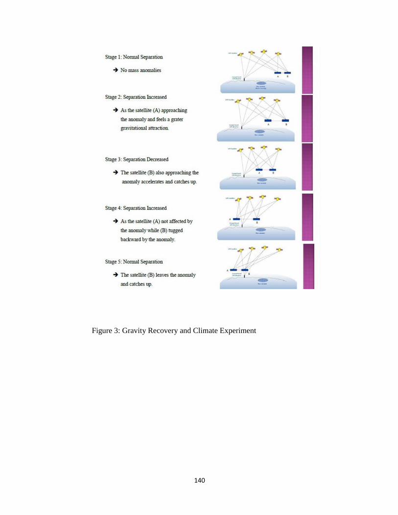
140
Figure 3: Gravity Recovery and Climate Experiment
141
(GRACE) mission concept.
1.5 GRACE Applications:
GRACE data has many applications, among others:
• Tracking water movement
• Tracking changes in ice sheets
• Tracking changes in the solid Earth.
Over the last decade, GRACE data has been successfully used to
monitor the individual components of the TWS. GRACE has been
widely used for:
(1) Estimating regional water storage variations in the Amazon
(Syed et al., 2005), Mississippi (Rodell et al., 2004; Syed et al.,
2005), Oklahoma (Swenson et al., 2008), Ob (Frappart et al., 2006),
and the Yangtze (Hu et al., 2006) River basins;
(2) Monitoring the elements of hydrologic cycles on sub-basin
scale in Africa (Ahmed et al., 2011);
(3) Characterizing terrestrial moisture changes in the Canadian
Prairie (Yirdaw et al., 2008);
(4) estimating the groundwater withdrawal rates in India (Tiwari
et al., 2009; Rodell etal., 2009) and California's Central Valley
(Famiglietti et al., 2011);
(5) Detecting water storage variations in the Three Gorges (Wang
142
et al., 2011) and Lake Victoria (Swenson and Wahr, 2009) reservoirs;
(6) Detecting flooding (Reager and Famiglietti, 2009) and
drought (Andersen et al., 2005; Yirdaw et al., 2008; Leblanc et al.,
2009; Agboma et al., 2009; Chen et al., 2010) potentials;
(1) Estimating the glacier melting rates in Alaska (Chen et al.,
2006), and ice sheet mass loss in Greenland (Velicogna and Wahr,
2005, 2006) and Antarctica (Velicogna et al., 2006; Chen et al., 2009).
1.1 GRACE Partners:
Here we are listing the main GRACE partners:
(1) The University of Texas at Austin-Center for Space Research (UT-
CSR), (2) GeoForschungsZentrum (GFZ), (3) National Aeronautics
and Space Association, Earth System Science Pathfinder Project, (4)
Deutschen Zentrum für Luft-und Raumfahrt (DLR), (5) Amarillo
Independent School District, (6) Analytical Mechanics Associates, (7)
Johns Hopkins University, Applied Physics Laboratory, (8) Astrium,
(9) DJO, DASA, Jena-Optronik, Gm, (10) Elizabeth Board of
Education, (11) Eurockot Launch Services, (12) European Space
Agency, Earth Sciences Division, (13) French Aeronautics and Space
Research Center (ONERA), (14) Killeen Independent School District,
(15) Llano Independent School District, (16) Massachusetts Institute
of Technology, Department of Earth, Atmospheric & Planetary
143
Sciences, (17) Messalonskee School System, (18) Mid Prairie
Community School District, (19) NASA/Goddard Space Flight Center,
(20) NASA Headquarters, (21) NASA/Jet Propulsion Laboratory, (22)
NASA/Kennedy Space Center, (23) NASA/Langley Research Center,
(24)Ohio State University, (25) Civil & Environmental Engineering
and Geodetic Science, (26) Space Systems Loral, (27) Stanford
Telecon, (28) Sunray Independent School District, (29) Technical
University of Denmark, (30) Texas Space Grant Consortium, and (31)
University of Colorado, Physics Department.
2. GRACE Data Products:
2.1 GRACE Data Levels:
As we discussed earlier, the long-term average distribution of the mass
within the Earth system determines its mean "static" gravity field. The
mean and time-variable gravity fields of the Earth affect the motion of
all Earth satellites. The motion of twin GRACE satellites (A and B)
are affected slightly differently since they occupy different positions in
space. These differences cause small relative motions between these
satellites (NASA, 2012, GRACE Mission. from
http://www2.csr.utexas.edu/grace/asdp.html). “The distance changes
are manifested as the change in time-of-flight of microwave signals
between the two satellites, which in turn is measured as the phase
144
change of the carrier signals. The influence of non-gravitational forces
on the inter-satellite range is measured using an accelerometer, and the
orientation of the spacecraft in space is measured using star cameras”
(NASA, 2012, GRACE Mission. from
http://www2.csr.utexas.edu/grace/asdp.html). The onboard GPS
receivers provide Science Data System (SDS) is responsible for
extraction of Earth gravity models is with the GRACE project (Fig. 4).
The SDS is distributed between University of Texas-Center of Space
Research (UT- CSR), Jet Propulsion Laboratory (JPL), and
GeoForschungsZentrum (GFZ). The SDS delivers monthly models of
Earth gravity field. At present, the GRACE data is divided into four
levels.
The raw data, collected from satellites, is calibrated and time-tagged in
a non-destructive (or reversible) sense and labeled Level-1A. Level-
1A data products are not distributed to the public (NASA, 2012,
GRACE Mission. from http://www2.csr.utexas.edu/grace/asdp.html).
These data undergo extensive and irreversible processing, and are
converted to edited and cleaned data products are 1-5 second rates.
The products labeled Level- 1B, include among others, the inter-
satellite range, range-rate, range-acceleration, the non- gravitational
accelerations from each satellite, the pointing estimates, the orbits, etc.
The Level- 1B products are processed to produce the monthly gravity
field estimates in the form of spherical harmonic coefficients. GRACE
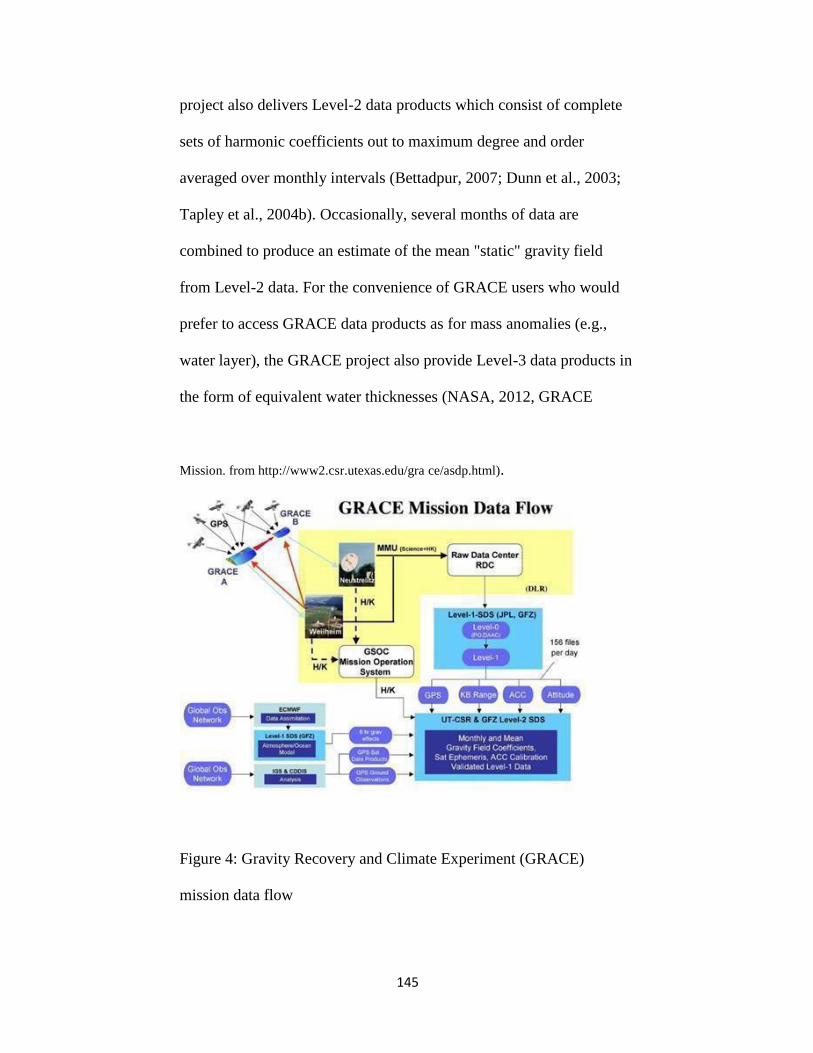
145
project also delivers Level-2 data products which consist of complete
sets of harmonic coefficients out to maximum degree and order
averaged over monthly intervals (Bettadpur, 2007; Dunn et al., 2003;
Tapley et al., 2004b). Occasionally, several months of data are
combined to produce an estimate of the mean "static" gravity field
from Level-2 data. For the convenience of GRACE users who would
prefer to access GRACE data products as for mass anomalies (e.g.,
water layer), the GRACE project also provide Level-3 data products in
the form of equivalent water thicknesses (NASA, 2012, GRACE
Mission. from http://www2.csr.utexas.edu/gra ce/asdp.html).
Figure 4: Gravity Recovery and Climate Experiment (GRACE)
mission data flow
146
2.1 Accessing GRACE Data:
2.1.1 Level-1B and Level-2:
Level-1B, Level-2 data, and GRACE Documentations are available at
1- ftp://podaac.jpl.nasa.gov/allData/grace
2.1.1 Level-3:
Level-3 data are available at:
1- http://grace.jpl.nasa.gov/data/
2- http://geoid.colorado.edu/grace/grace.php
3- http://icgem.gfz-potsdam.de/ICGEM/ICGEM.html
2.2 GRACE Data Format:
Level-2 GRACE data are represented as a complete set of harmonic
coefficients out to maximum degree and order averaged over monthly
intervals. These data represent the GRACE anomalies after
subtracting the background models (Fig. 5). The Background Model
consists of mathematical models and the associated parameter values,
which are used along with numerical techniques to predict the best-
known value for the observable (in this case, the inter-satellite range
or its derivatives). The Background Model encompasses both satellite
dynamics and measurements. This model changes with the evolution
of processing methods. The spherical harmonic coefficient at a given
time is given by:
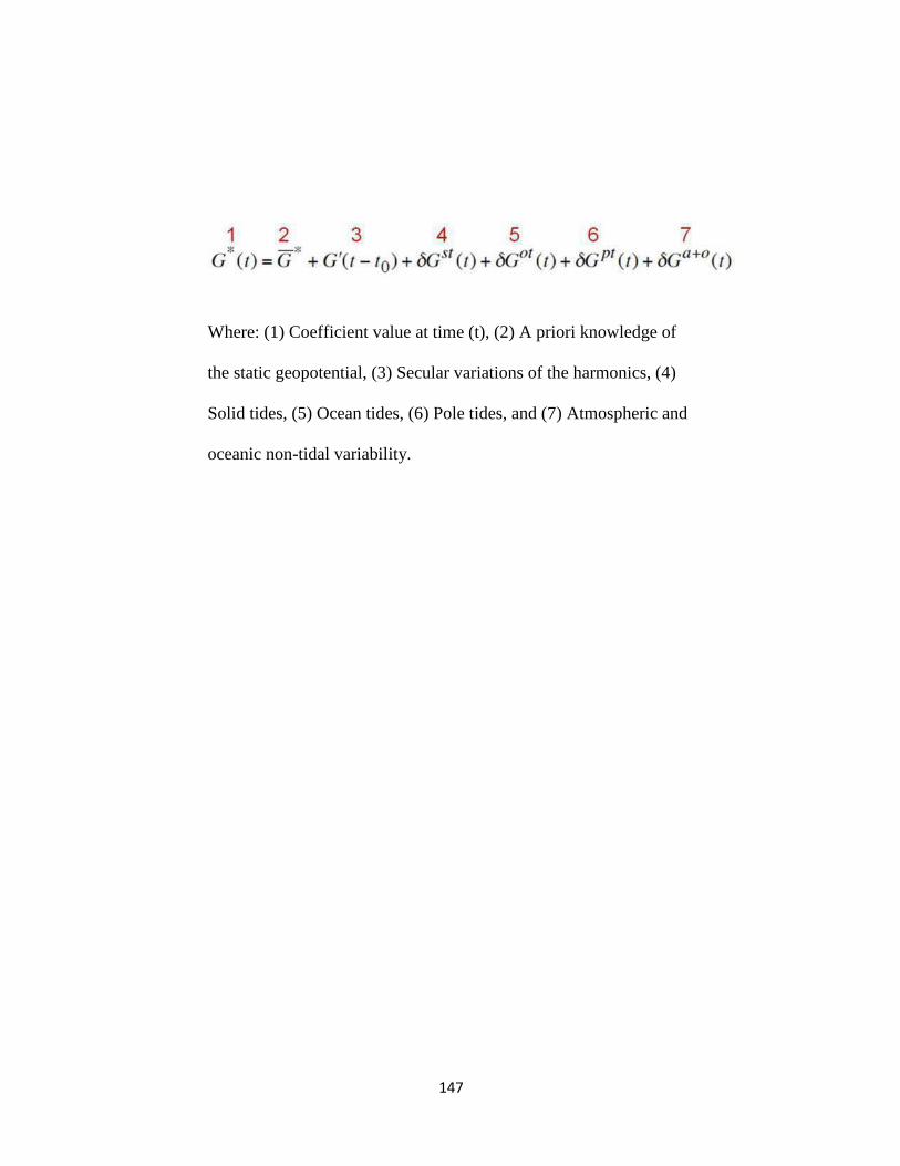
147
Where: (1) Coefficient value at time (t), (2) A priori knowledge of
the static geopotential, (3) Secular variations of the harmonics, (4)
Solid tides, (5) Ocean tides, (6) Pole tides, and (7) Atmospheric and
oceanic non-tidal variability.
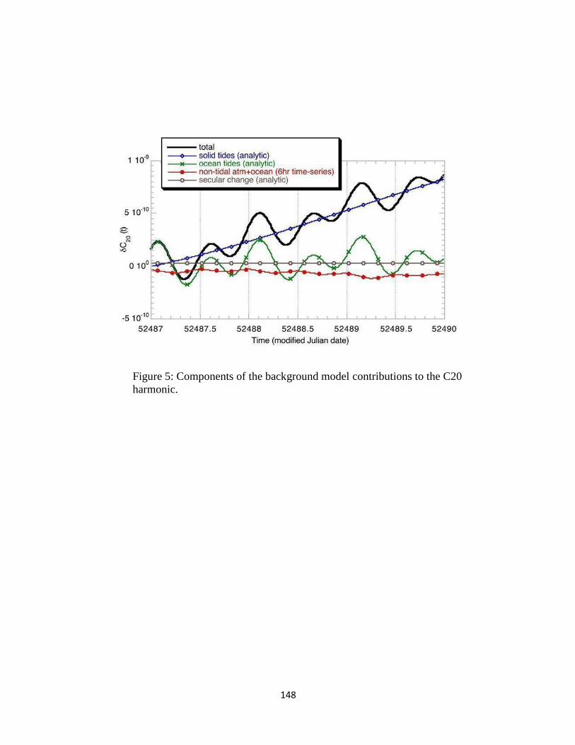
148
Figure 5: Components of the background model contributions to the C20
harmonic.
149
A GRACE Level-2 gravity field product is a set of spherical
harmonic coefficients of the exterior geopotential. Level-2 data are
produced by CSR, JPL and GFZ centers. A product name is specified
as:
PID-2_YYYYDOY-YYYYDOY_dddd_sssss_mmmm_rrrr Where:
PID: is 3-character product identification mnemonic
-2: denotes a GRACE Level-2 product
YYYYDOY-YYYYDOY: specifies the date range (in year and day-of-year
format) of the data used in creating this product.
dddd is the (leading-zero-padded) number of calendar days from which data
was used in creating the product.
sssss is an institution-specific string.
mmmm is a 4-character free string (e.g., used for distinguishing constrained
from unconstrained solutions).
rrrr: is a 4-digit (leading-zero-padded) release number (0000, 0001, … )
The Product Identifier mnemonic (PID) is made up of one of the following
values for each of its three characters:
1st Character:
150
= G: Geopotential coefficients. 2nd Character:
= S: Estimate made from only GRACE data.
=C: Combination estimate from GRACE and terrestrial gravity information.
= E: Any background model specified as a time-series.
= A: Average of any background model over a period. 3rd Character:
= M: Estimate of the Static field.
= U: Geopotential estimate relative to the background gravity model.
= T: Total background gravity model except for static background model.
= A: non-tidal atmosphere.
= B: non-tidal Oceans.
= C: combination of non-tidal atmosphere and ocean.
= D: bottom-pressure over oceans, zero over land. Example of the GSM file
is shown in Figure 6
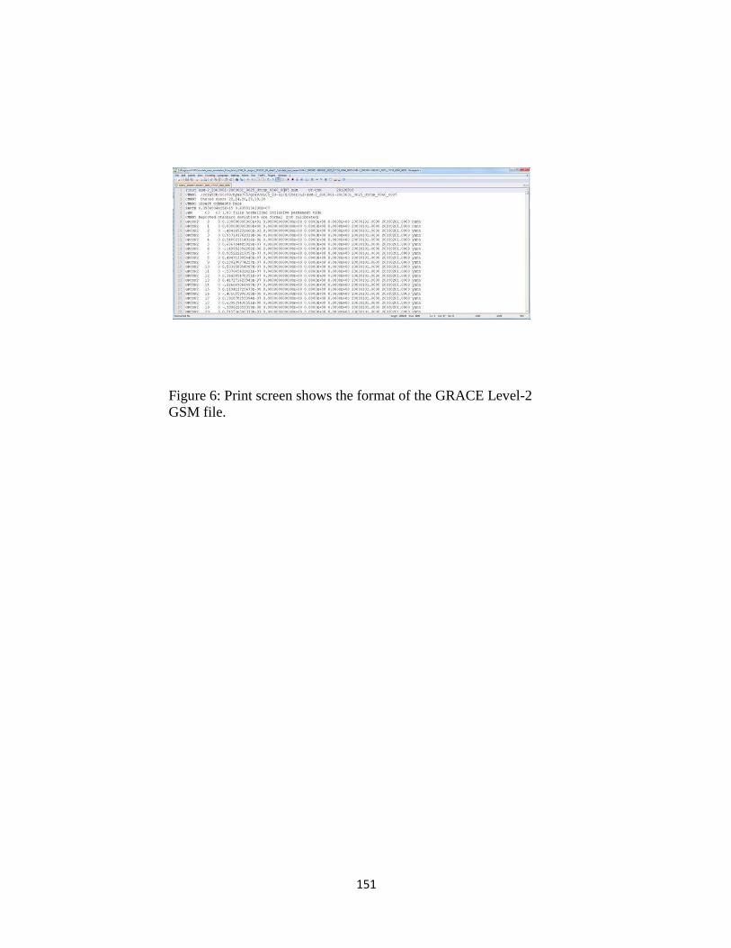
151
Figure 6: Print screen shows the format of the GRACE Level-2
GSM file.
152
2.1 Spherical Harmonics:
GRACE level-2 data are in the form of spherical harmonics.
Spherical harmonics are used to express values that vary sinusoidally
in both latitude and longitude direction. Examples of these include
the gravity and magnetic fields of the Earth, the geoid, earth
topography, electron distribution around the atom, ..). The spherical
harmonic coefficients are given regarding degree (ℓ) and order (m).
m = is the number of nodes (great circles) in the longitudinal
direction, where, angle (ɸ) increases East from the Greenwich, and it
ranges between 0 and 2π. The value (ℓ−m) gives the number of nodes
in the latitudinal sense. Where the angle (θ) increases from the North
Pole, and it ranges from 0 to π (Fig. 7). Visualizations of the spherical
harmonics are given at the GFZ website: http://icgem.gfz-
potsdam.de/ICGEM/potato/Tutorial.html.
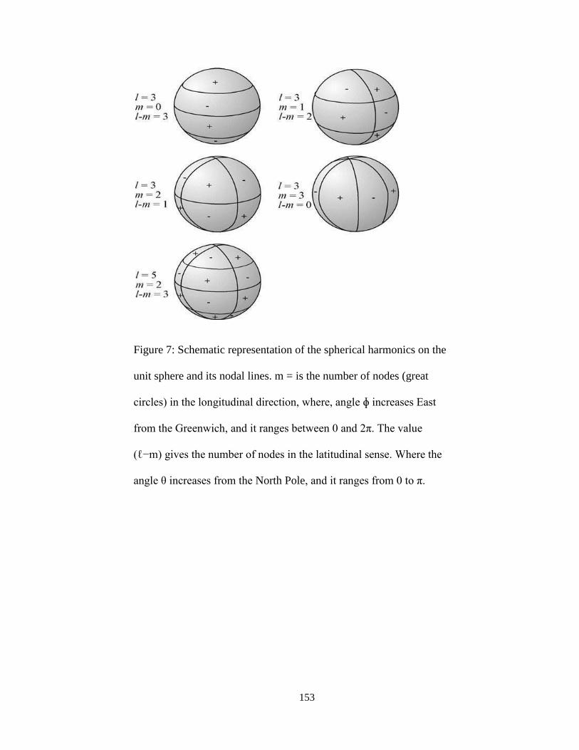
153
Figure 7: Schematic representation of the spherical harmonics on the
unit sphere and its nodal lines. m = is the number of nodes (great
circles) in the longitudinal direction, where, angle ɸ increases East
from the Greenwich, and it ranges between 0 and 2π. The value
(ℓ−m) gives the number of nodes in the latitudinal sense. Where the
angle θ increases from the North Pole, and it ranges from 0 to π.
154
3. Processing of GRACE Data:
In this section, we are introducing, in brief, the general steps that
most of the researchers are using in processing of GRACE level-2
data.
3.1 Removal of the Temporal Mean:
The GRACE level-2 solutions are represented regarding fully
normalized spherical harmonic decompositions up to degree (l) and
order (m) of 60. The time-variable component of the gravity field
solutions should be calculated by removing the long-term mean (Clm
(t), Slm (t)) of the Stokes coefficients from each monthly (Clm (t),
Slm (t)) value to get the temporal variations in these coefficients ( (
Clm (t), Slm (t)) . The reason for removing the mean field is that it is
dominated by the static density distribution inside the solid Earth
(Wahr et al., 1998).
3.2 Spectral Filtering (Destripping):
After the temporal mean removal, the correlated errors (long, linear,
north to south oriented features) also called “stripes” should be
reduced by applying describing methods developed by Swenson and
Wahr (2006). The presence of stripes implies spatial correlations in
the gravity field coefficients at higher degree (short wavelength
components). Swenson and Wahr (2006) show how, at a single
higher (m>8) order, the even (or odd) coefficients values at each
155
degree tend to form smooth curves. Their filter, a moving window
quadratic polynomial, was used to isolate and remove smoothly
varying coefficients of the same parity. In this study, the least square
method was used to fit a 4th order polynomial for the odd degree and
the even degree separately, then to subtract those polynomials from
the original coefficients to leave the residuals (Cˆlm (t), Cˆlm (t)).
3.3 Spatial Averaging (Gaussian Smoothing):
At this point, we have a set of gravity coefficient anomalies for each
month (∆Cˆlm (t),∆Cˆlm (t)) that have been described and ready to
compute mass anomalies. Several studies have used GRACE monthly
solutions to make estimates of water storage variability, both on land
and in the oceans (Chambers et al., 2004; Chen et al., 2005;
Ramillien et al., 2005; Swenson and Milly, 2006; Tamisiea et al.,
2005; Tapley et al., 2004b; Velicogna and Wahr, 2005; Wahr et al.,
2004).
We will compute maps of water storage anomalies over the land ( ∆σ
(θ,φ,t) ) directly as:
156
Where is ρave the average density of the Earth (5517 kg m-3), ae is
the mean equatorial radius of the Earth, θ is the geographic latitude,φ
is the longitude, Plm are the fully-normalized
Associated Legendre Polynomials of degree l and order m and r is the
Gaussian averaging radius, and kl are elastic/load Love numbers of
degree l. The later was calculated via linear interpolation of the
original data computed by Han and Wahr (1995).
The spatial averaging, or smoothing, of GRACE data, is necessary to
reduce the contribution of noisy short wavelength components of the
gravity field solutions. We will generate 0.5° × 0.5° equivalent water
thickness grids using a Gaussian averaging radius of 200 km.
3.4 GRACE Errors:
Errors in GRACE-derived TWS fall into two main categories (Wahr
et al., 2006): (1) Errors in monthly GRACE solutions. These include
measurement and processing errors, aliasing errors related to the
short-period (sub-monthly) variations and errors in the European
Centre for Medium-Range Weather Forecasts (ECMWF) models
used for atmospheric corrections of
GRACE data; (2) Errors due to changes caused by factors other than
continental water storage (i.e., leakage errors).The leakage errors can
come from time-variable mass anomalies either vertically above or
157
below, or from mass anomalies off to the side of the area of interest.
The time variable gravity below the area of interest might include the
gravity signal related to un-modeled mass variations in the Earth’s
interior while that above the area of interest might be related to errors
in the atmospheric models (ECMWF). Leakage errors can also come
from continental water storage signals where it comes from water
storage outside of the region of interest. The measurement errors in
GRACE data (type 1) exhibits a zonally banded pattern and varies
with the Gaussian smoothing function used and with the latitude. At
lower latitudes, a maximum error of ~36 mm (equivalent water
thickness) was obtained with a Gaussian radius of 300 km whereas an
error of ~28 mm was obtained when using a Gaussian radius of 750
km was adopted.
Poleward, the error decreases to <15 mm (Landerer and Swenson,
2012; Wahr et al., 2006).
Estimates of TWS variations suffer from signal degradation due to
noise. The noise is manifested as (1) random errors that increase as a
function of spherical harmonic spectral degree (Wahr et al., 2006),
and (2) systematic errors that are correlated within a particular
spectral order (Swenson and Wahr, 2006).
Several filtering techniques are used to damp or isolate and remove
the GRACE-derived TWS errors. The problem with most of those
158
techniques is that the filters also modify the actual geophysical signal
that the researchers are interested in. The following section explains
the methods used to scale GRACE TWS data to account for the effect
of the filter on the GRACE signal.
3.5 Scaling GRACE TWS Data
The scaling process is supposed to take care of the GRACE TWS
errors that result from applying the following filters and/or
truncations: (1) destriping filter designed to remove systematic errors
that are characterized by correlations between certain spherical
harmonic coefficients (Swenson and Wahr, 2006); (2) Gaussian
smoothing filter when applied, it smoothes, but reduces the spatial
resolution of GRACE observations by damping the higher degree
coefficients (Wahr et al., 1998); and (3) truncation of the monthly
GRACE solutions where GRACE gravity solutions
are typically truncated at a spectral degree (lmax ≤ 60; wavelength of
~330 km). This truncation means that GRACE cannot resolve signals
with spatial variability finer than 330 km (Wahr et al., 1998; Wahr et
al., 2006).
159
References:
• Bettadpur, S., 2006, GRACE level-2 gravity field product
user handbook: Center for Space Research, The University of Texas
at Austin.
• Bettadpur, S., 2007, GRACE Product Specification
Document: Center for Space Research The University of Texas at
Austin.
• Chambers, D.P., Wahr, J., and Nerem, R.S., 2004,
Preliminary observations of global ocean mass with GRACE:
Geophysical Research Letters, v. 31, L13310.
• Chen, J., Wilson, C., Famiglietti, J., and Rodell, M., 2005,
Spatial sensitivity of the Gravity Recovery and Climate Experiment
(GRACE) time-variable gravity observations: Journal of Geophysical
Research, v. 110, B08408, doi: 10.1029/2004JB003536.
• Dunn, C., Bertiger, W., Bar-Sever, Y., Desai, S., Haines, B.,
Kuang, D., Franklin, G., Harris, I., Kruizinga, G., Meehan, T., Nandi,
S., Nguyen, D., Rogstad, T., Thomas, J.B., Tien, J., Romans, L.,
Watkins, M., Wu, S.-C., Bettadpur, S., and Kim, J., 2003, Instrument
of GRACE: GPS Augments Gravity Measurements: GPS World, v.
14, p. 16-28.
• Flechtner, F., 2005, GFZ Level-2 Processing Standards
Document for Level-2Product Release 0003: GeoForschungszentrum

160
Potsdam: Geodesy and Remote Sensing.
• Han, D., and Wahr, J., 1995, The viscoelastic relaxation of a
realistically stratified Earth, and a further analysis of postglacial
rebound: Geophysical Journal International, v. 120, p. 287– 311.
• Ramillien, G., Frappart, F., Cazenave, A., and Gnter, A.,
2005, Time variations of land water storage from an inversion of 2
years of GRACE geoids: Earth and Planetary Science Letters, v.
253, p. 283– 301.
• Schmidt, R., Flechtner, F., Meyer, U., Neumayer, K.H.,
Dahle, C., König, R., and Kusche, J., 2008, Hydrological Signals
Observed by the GRACE Satellites: Survey in Geophysics, v. 29,
p. 319-334, doi: 10.1007/s10712-008-9033-3.
• Swenson, S.C., and Milly, P.C.D., 2006, Climate model
biases in seasonality of continental water storage revealed by
satellite gravimetry: Water Resources Research, v.42, W03201.
• Tamisiea, M.E., Leuliette, E.W., Davis, J.L., and Mitrovica,
J.X., 2005, Constraining hydrological and cryospheric mass flux in
southeastern Alaska using space-based gravity measurements:
Geophysical Research Letters, v. 32, L20501.
• Tapley, B.D., Bettadpur, S., Ries, J.C., Thompson, P.F., and
Watkins, M.M., 2004a, GRACE Measurements of Mass
Variability in the Earth System: Science, v. 305, p. 503–505, doi:
161
10.1126/science.1099192.
• Tapley, B.D., Bettadpur, S., Watkins, M., and Reigber, C.,
2004b, The Gravity Recovery and Climate Experiment: Mission
overview and early results: Geophysical Research Letters, v. 31,
L09607.
• Velicogna, I., and Wahr, J., 2005, Ice mass balance in
Greenland from GRACE: Journal of Geophysical Research, v. 32,
L18505, doi: 10.1029/2005GL023955.
162
APPENDIX B
Scientific Methods
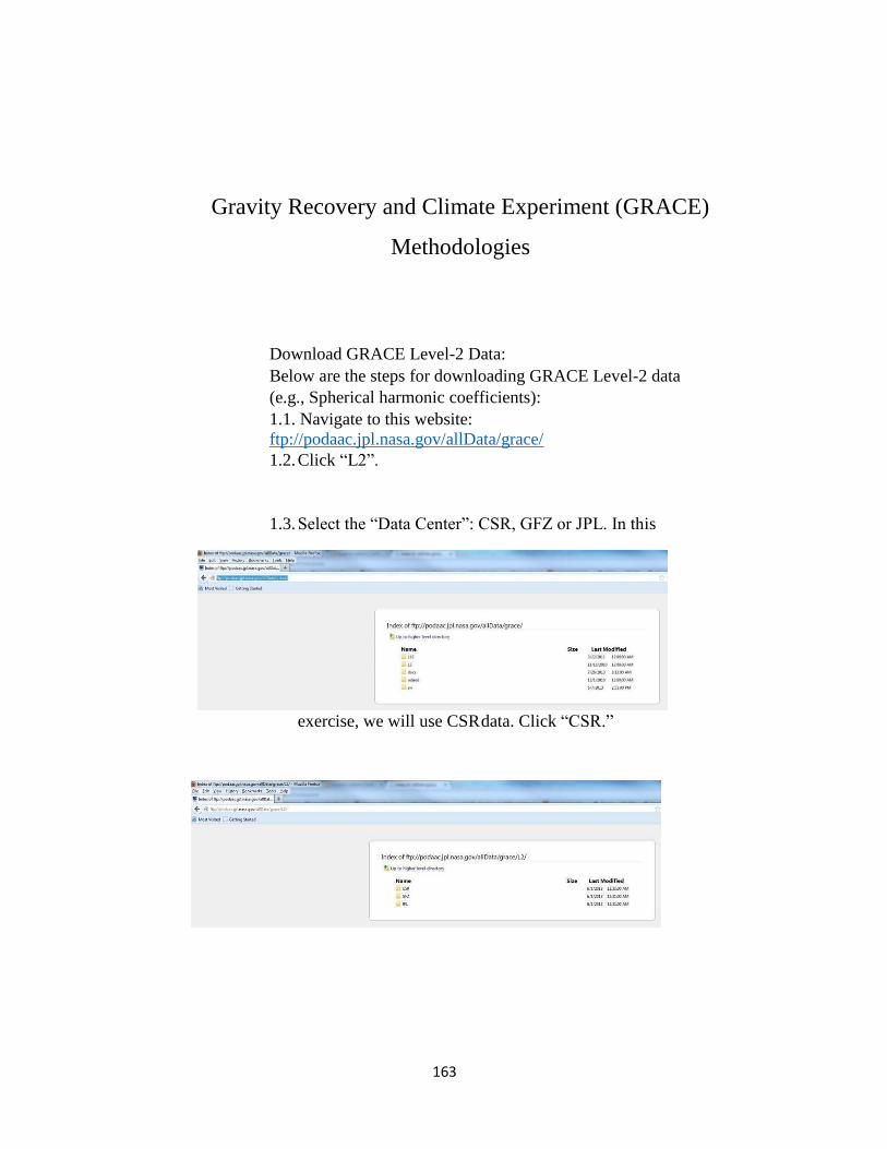
163
Gravity Recovery and Climate Experiment (GRACE)
Methodologies
Download GRACE Level-2 Data:
Below are the steps for downloading GRACE Level-2 data
(e.g., Spherical harmonic coefficients):
1.1. Navigate to this website:
ftp://podaac.jpl.nasa.gov/allData/grace/
1.2. Click “L2”.
1.3. Select the “Data Center”: CSR, GFZ or JPL. In this
exercise, we will use CSR data. Click “CSR.”
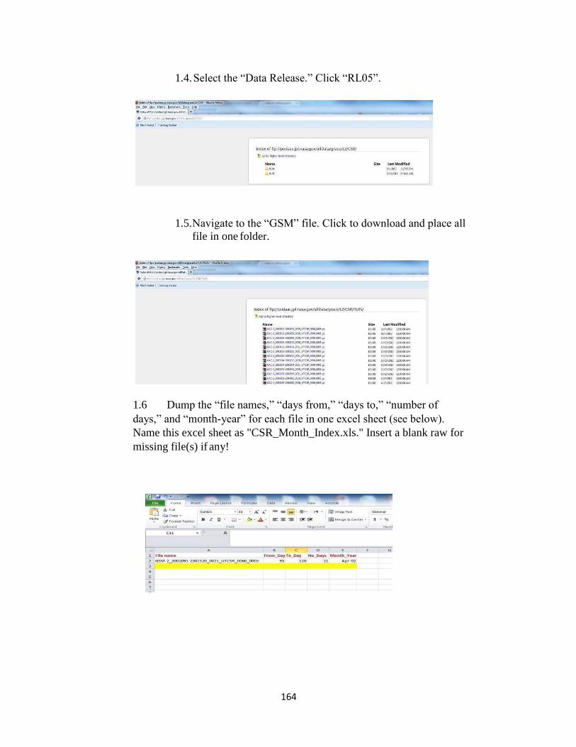
164
1.4. Select the “Data Release.” Click “RL05”.
1.5. Navigate to the “GSM” file. Click to download and place all
file in one folder.
1.6 Dump the “file names,” “days from,” “days to,” “number of
days,” and “month-year” for each file in one excel sheet (see below).
Name this excel sheet as "CSR_Month_Index.xls." Insert a blank raw for
missing file(s) if any!
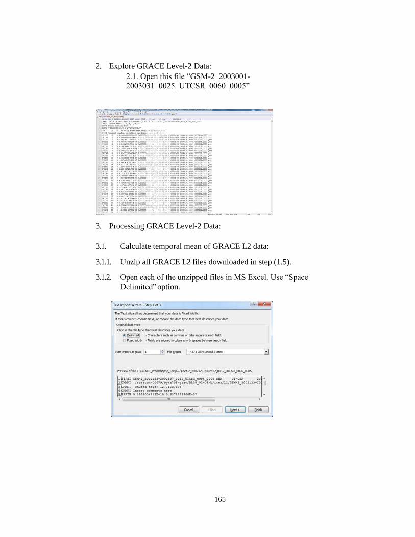
165
2. Explore GRACE Level-2 Data:
2.1. Open this file “GSM-2_2003001-
2003031_0025_UTCSR_0060_0005”
3. Processing GRACE Level-2 Data:
3.1. Calculate temporal mean of GRACE L2 data:
3.1.1. Unzip all GRACE L2 files downloaded in step (1.5).
3.1.2. Open each of the unzipped files in MS Excel. Use “Space
Delimited” option.
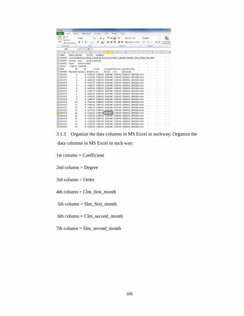
166
3.1.3 Organize the data columns in MS Excel in such way: Organize the
data columns in MS Excel in such way:
1st column = Coefficient
2nd column = Degree
3rd column = Order
4th column = Clm_first_month
5th column = Slm_first_month
6th column = Clm_second_month
7th column = Slm_second_month
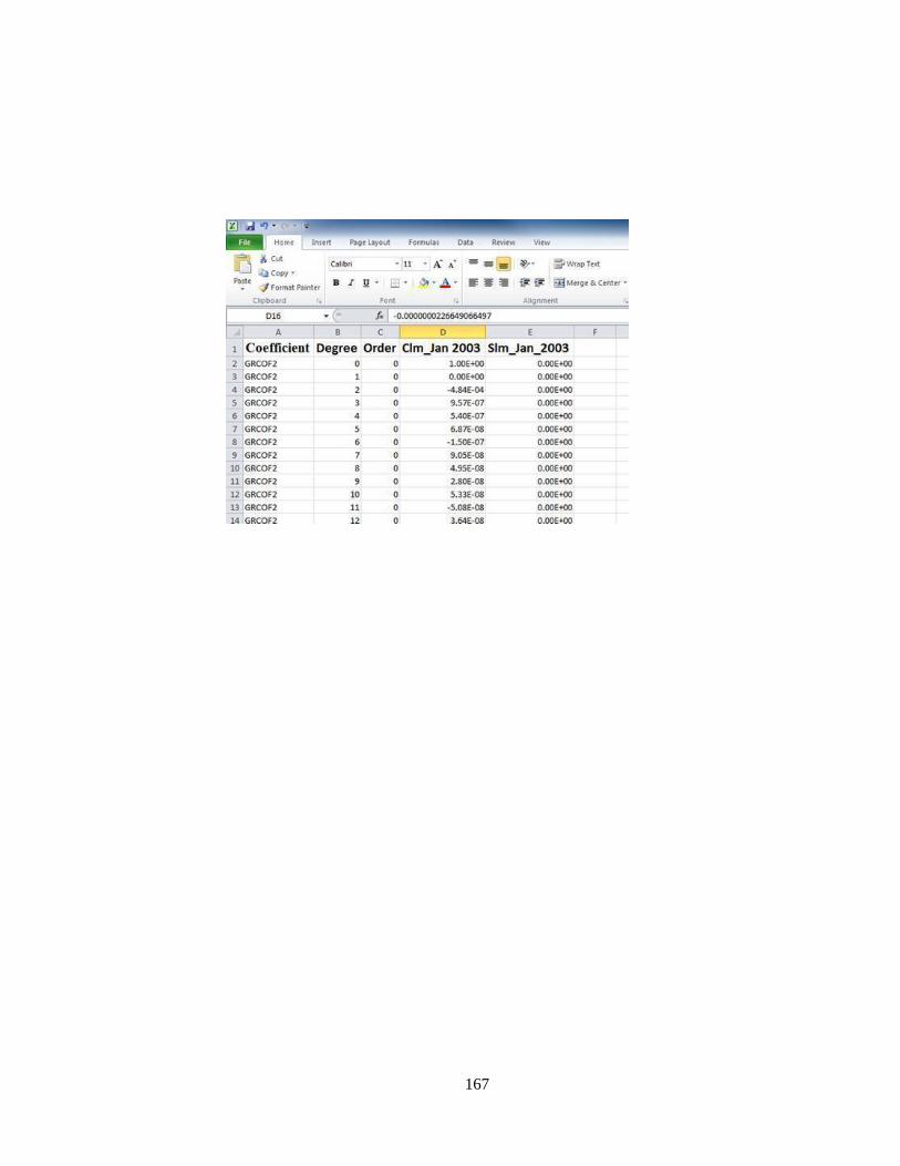
167
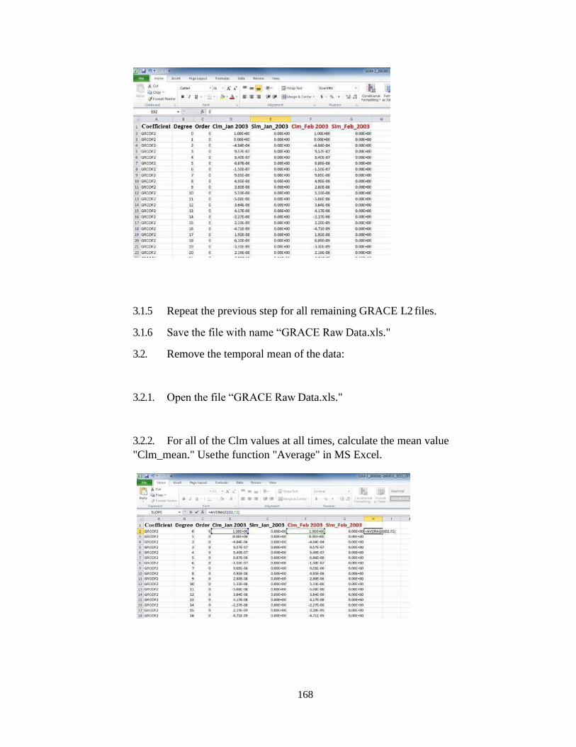
168
3.1.5 Repeat the previous step for all remaining GRACE L2 files.
3.1.6 Save the file with name “GRACE Raw Data.xls."
3.2. Remove the temporal mean of the data:
3.2.1. Open the file “GRACE Raw Data.xls."
3.2.2. For all of the Clm values at all times, calculate the mean value
"Clm_mean." Use the function "Average" in MS Excel.
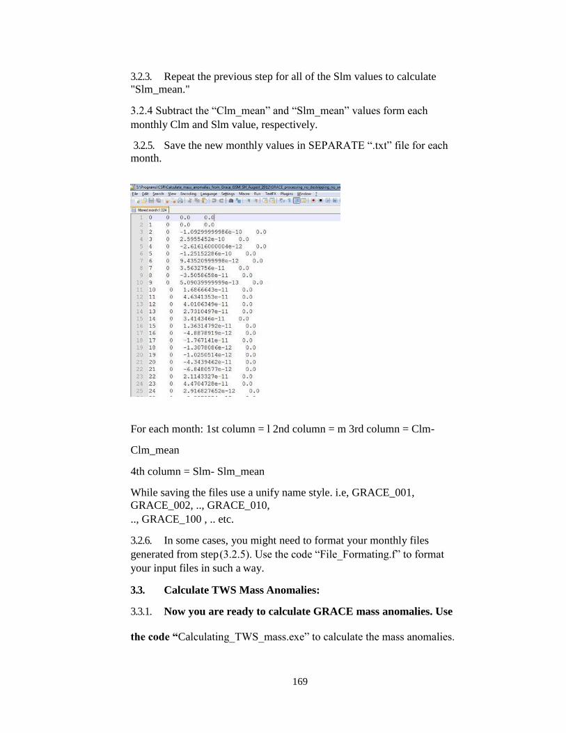
169
3.2.3. Repeat the previous step for all of the Slm values to calculate
"Slm_mean."
3.2.4 Subtract the “Clm_mean” and “Slm_mean” values form each
monthly Clm and Slm value, respectively.
3.2.5. Save the new monthly values in SEPARATE “.txt” file for each
month.
For each month: 1st column = l 2nd column = m 3rd column = Clm-
Clm_mean
4th column = Slm- Slm_mean
While saving the files use a unify name style. i.e, GRACE_001,
GRACE_002, .., GRACE_010,
.., GRACE_100 , .. etc.
3.2.6. In some cases, you might need to format your monthly files
generated from step (3.2.5). Use the code “File_Formating.f” to format
your input files in such a way.
3.3. Calculate TWS Mass Anomalies:
3.3.1. Now you are ready to calculate GRACE mass anomalies. Use
the code “Calculating_TWS_mass.exe” to calculate the mass anomalies.
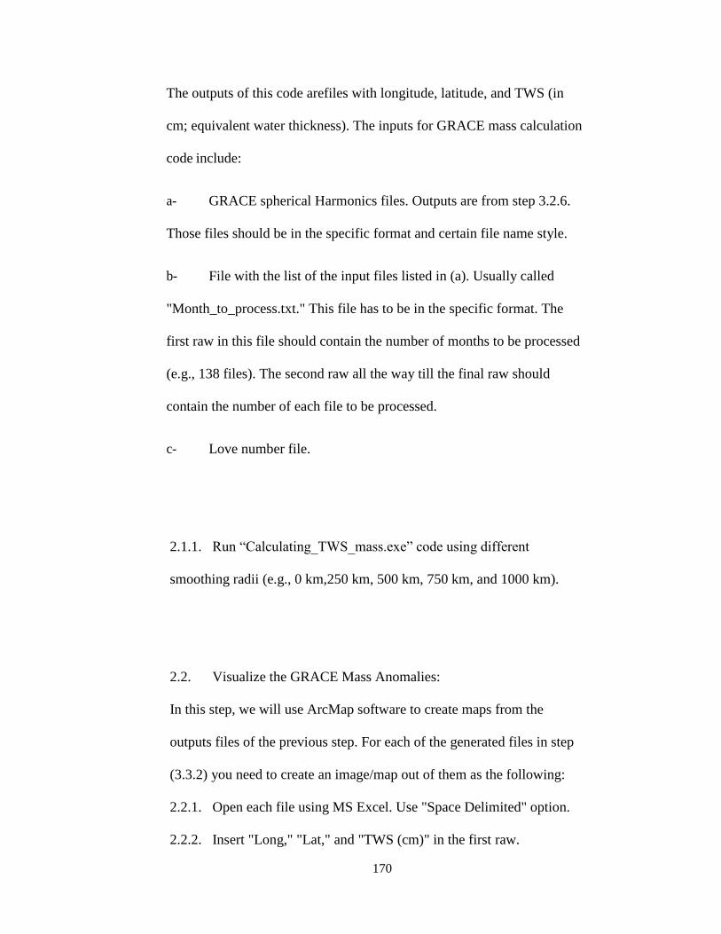
170
The outputs of this code arefiles with longitude, latitude, and TWS (in
cm; equivalent water thickness). The inputs for GRACE mass calculation
code include:
a- GRACE spherical Harmonics files. Outputs are from step 3.2.6.
Those files should be in the specific format and certain file name style.
b- File with the list of the input files listed in (a). Usually called
"Month_to_process.txt." This file has to be in the specific format. The
first raw in this file should contain the number of months to be processed
(e.g., 138 files). The second raw all the way till the final raw should
contain the number of each file to be processed.
c- Love number file.
2.1.1. Run “Calculating_TWS_mass.exe” code using different
smoothing radii (e.g., 0 km,250 km, 500 km, 750 km, and 1000 km).
2.2. Visualize the GRACE Mass Anomalies:
In this step, we will use ArcMap software to create maps from the
outputs files of the previous step. For each of the generated files in step
(3.3.2) you need to create an image/map out of them as the following:
2.2.1. Open each file using MS Excel. Use "Space Delimited" option.
2.2.2. Insert "Long," "Lat," and "TWS (cm)" in the first raw.
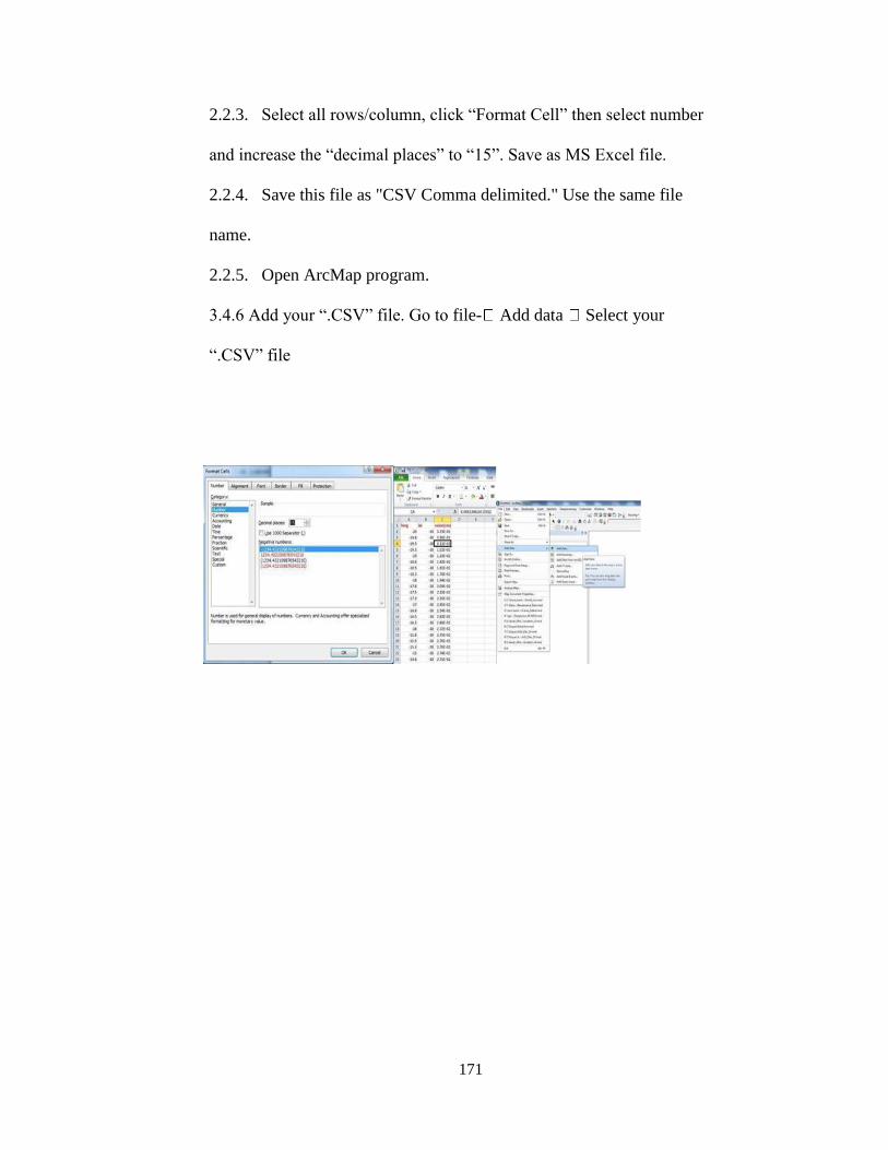
171
2.2.3. Select all rows/column, click “Format Cell” then select number
and increase the “decimal places” to “15”. Save as MS Excel file.
2.2.4. Save this file as "CSV Comma delimited." Use the same file
name.
2.2.5. Open ArcMap program.
3.4.6 Add your “.CSV” file. Go to file- Add data Select your
“.CSV” file
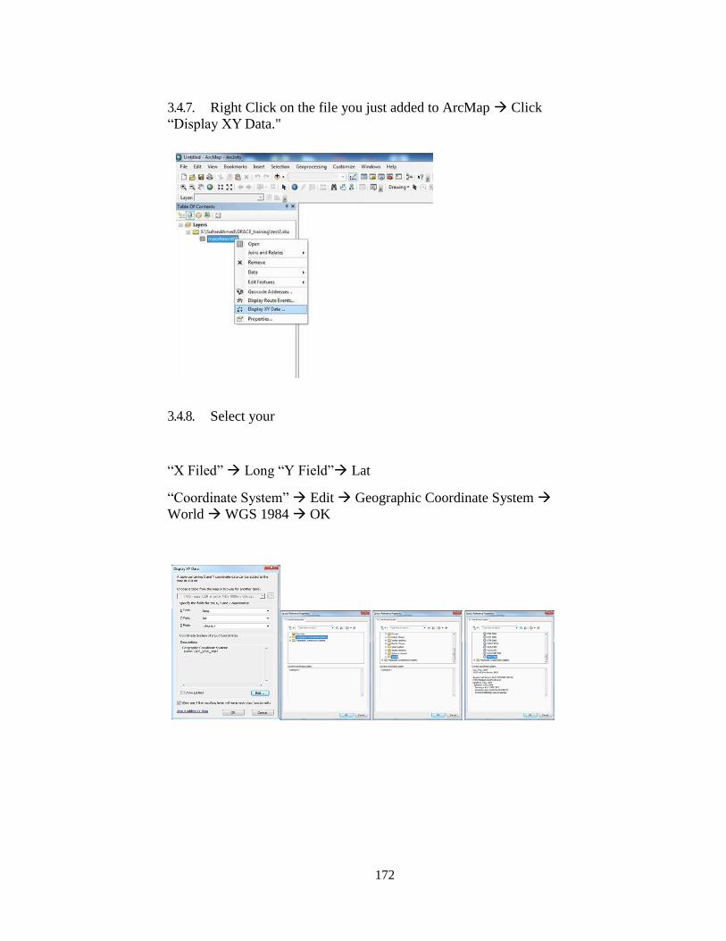
172
3.4.7. Right Click on the file you just added to ArcMap Click
“Display XY Data."
3.4.8. Select your
“X Filed” Long “Y Field” Lat
“Coordinate System” Edit Geographic Coordinate System
World WGS 1984 OK
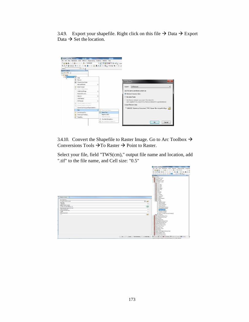
173
3.4.9. Export your shapefile. Right click on this file Data Export
Data Set the location.
3.4.10. Convert the Shapefile to Raster Image. Go to Arc Toolbox
Conversions Tools To Raster Point to Raster.
Select your file, field "TWS(cm)," output file name and location, add
".tif" to the file name, and Cell size: "0.5"
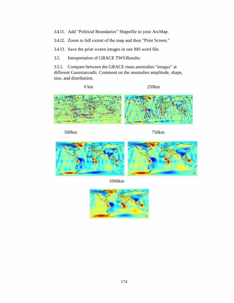
174
3.4.11. Add “Political Boundaries” Shapefile to your ArcMap.
3.4.12. Zoom to full extent of the map and then “Print Screen."
3.4.13. Save the print screen images in one MS word file.
3.5. Interpretation of GRACE TWS Results:
3.5.1. Compare between the GRACE mass anomalies “images” at
different Gaussian radii. Comment on the anomalies amplitude, shape,
size, and distribution.
0 km 250km
500km 750km
1000km
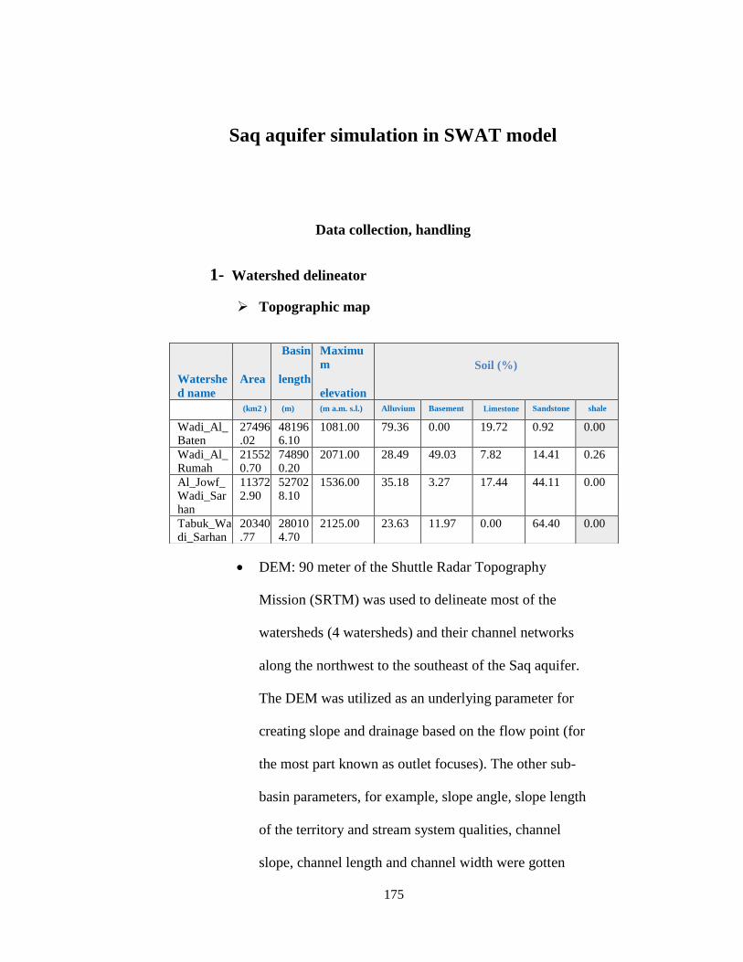
175
Saq aquifer simulation in SWAT model
Data collection, handling
1- Watershed delineator
Topographic map
DEM: 90 meter of the Shuttle Radar Topography
Mission (SRTM) was used to delineate most of the
watersheds (4 watersheds) and their channel networks
along the northwest to the southeast of the Saq aquifer.
The DEM was utilized as an underlying parameter for
creating slope and drainage based on the flow point (for
the most part known as outlet focuses). The other sub-
basin parameters, for example, slope angle, slope length
of the territory and stream system qualities, channel
slope, channel length and channel width were gotten
Watershe
d name
Area
Basin
length
Maximu
m
elevation
Soil (%)
(km2 ) (m) (m a.m. s.l.) Alluvium Basement Limestone Sandstone shale
Wadi_Al_Baten
27496.02
481966.10
1081.00 79.36 0.00 19.72 0.92 0.00
Wadi_Al_Rumah
215520.70
748900.20
2071.00 28.49 49.03 7.82 14.41 0.26
Al_Jowf_Wadi_Sarhan
113722.90
527028.10
1536.00 35.18 3.27 17.44 44.11 0.00
Tabuk_Wadi_Sarhan
20340.77
280104.70
2125.00 23.63 11.97 0.00 64.40 0.00
176
from DEM handling in the SWAT model.
Stream delineation information for each watershed as the
following
Outlet definition : The outlet of Wadi_Al_Baten and
Wadi_Al_Rumah are in the Golf of Arab and for
Al_Jowf_Wadi_Sarhan and Tabuk_Wadi_Sarhan outlets
are in the Gulf of Aqaba.
Calculation of sub-basin parameters
1- HRU analysis
• In SWAT, a basin is delineated into sub-basins, which are
then further subdivided into Hydrological Respond Units
(HRUs). The HRUs consist of homogeneous land use and
soil type. The primary input, (DEM) digital elevation
model, (LULC) land-use/land- cover, soil data and
hydrogeological data such daily rainfall (mm), temperature
(˚C), solar (MJ/m^2), Relative Humidity (fraction), and
Wind (m/s).
• All that variables have been used for the initial SWAT
model set-up SRTM elevation data presented in GRID
can be downloaded for the whole world
(http://dwtkns.com/srtm/). The SRTM data were
provided into a WGS_1984_UTM_Zone_37N projection
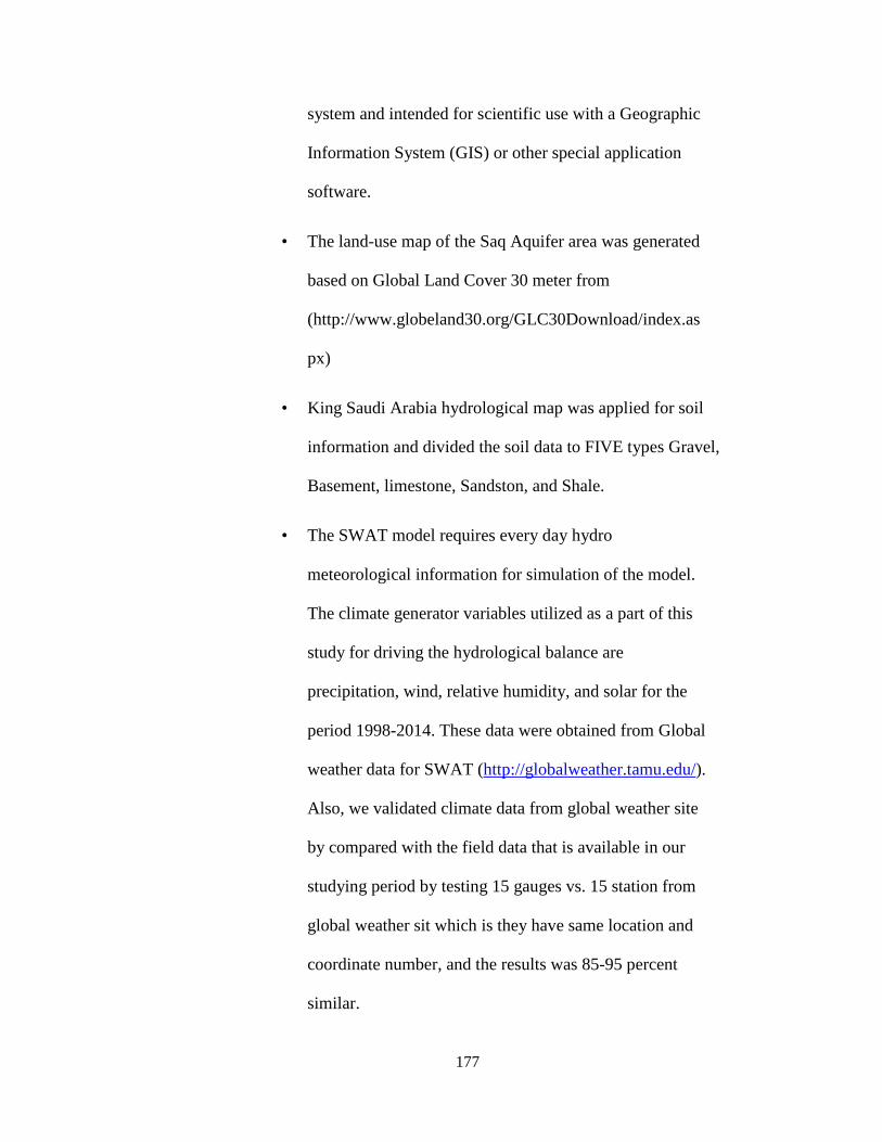
177
system and intended for scientific use with a Geographic
Information System (GIS) or other special application
software.
• The land-use map of the Saq Aquifer area was generated
based on Global Land Cover 30 meter from
(http://www.globeland30.org/GLC30Download/index.as
px)
• King Saudi Arabia hydrological map was applied for soil
information and divided the soil data to FIVE types Gravel,
Basement, limestone, Sandston, and Shale.
• The SWAT model requires every day hydro
meteorological information for simulation of the model.
The climate generator variables utilized as a part of this
study for driving the hydrological balance are
precipitation, wind, relative humidity, and solar for the
period 1998-2014. These data were obtained from Global
weather data for SWAT (http://globalweather.tamu.edu/).
Also, we validated climate data from global weather site
by compared with the field data that is available in our
studying period by testing 15 gauges vs. 15 station from
global weather sit which is they have same location and
coordinate number, and the results was 85-95 percent
similar.
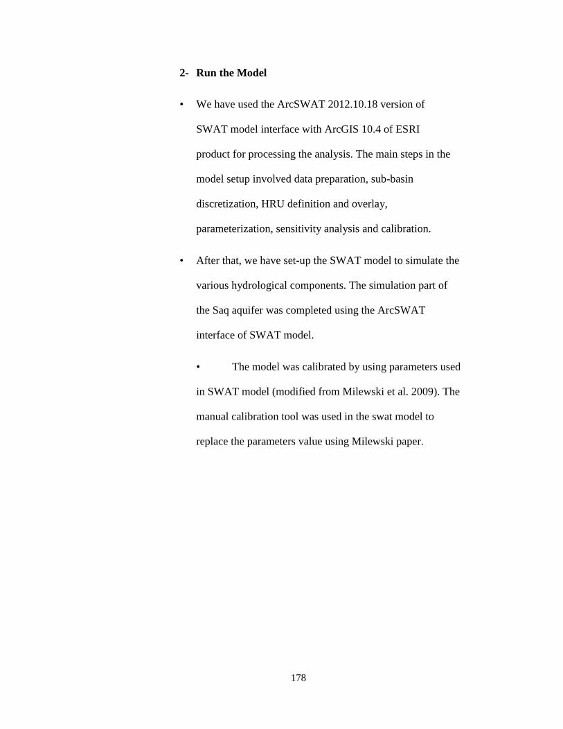
178
2- Run the Model
• We have used the ArcSWAT 2012.10.18 version of
SWAT model interface with ArcGIS 10.4 of ESRI
product for processing the analysis. The main steps in the
model setup involved data preparation, sub-basin
discretization, HRU definition and overlay,
parameterization, sensitivity analysis and calibration.
• After that, we have set-up the SWAT model to simulate the
various hydrological components. The simulation part of
the Saq aquifer was completed using the ArcSWAT
interface of SWAT model.
• The model was calibrated by using parameters used
in SWAT model (modified from Milewski et al. 2009). The
manual calibration tool was used in the swat model to
replace the parameters value using Milewski paper.
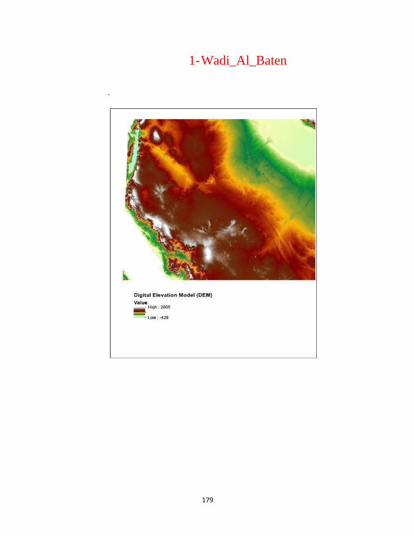
179
1- Wadi_Al_Baten
`
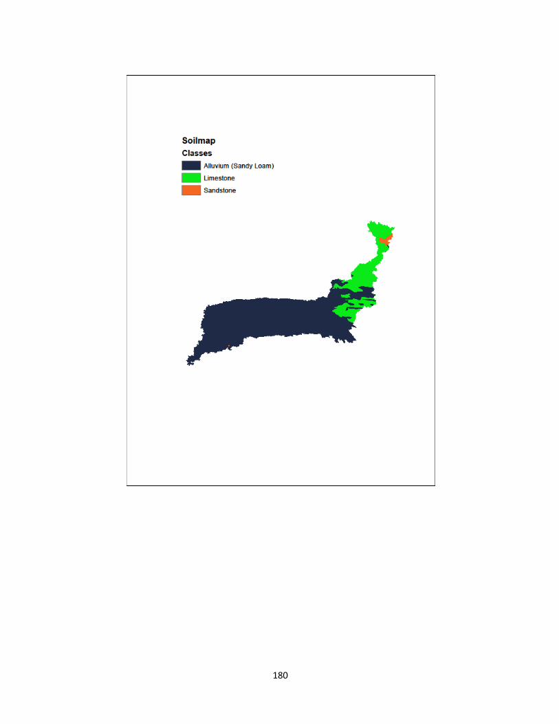
180
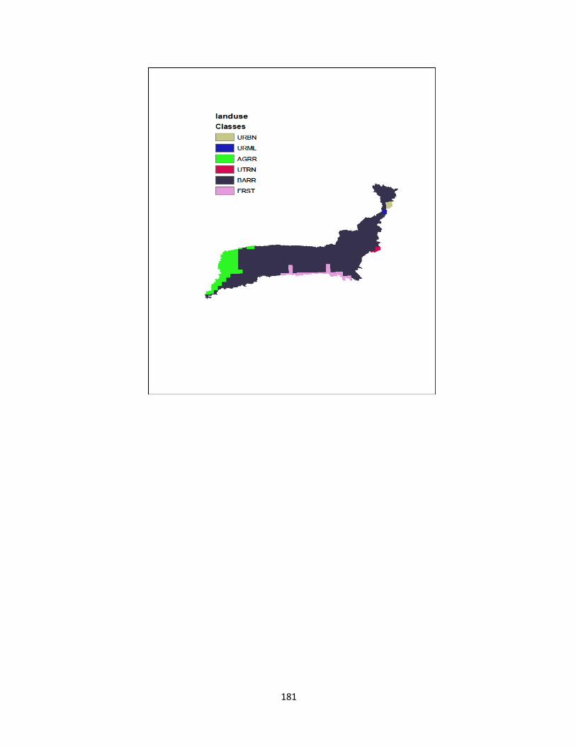
181
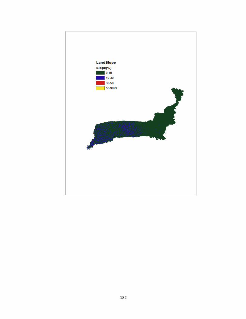
182
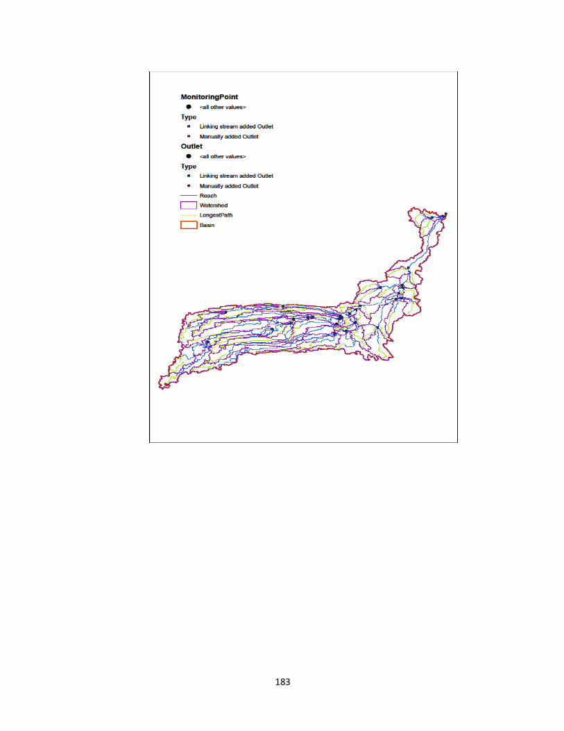
183
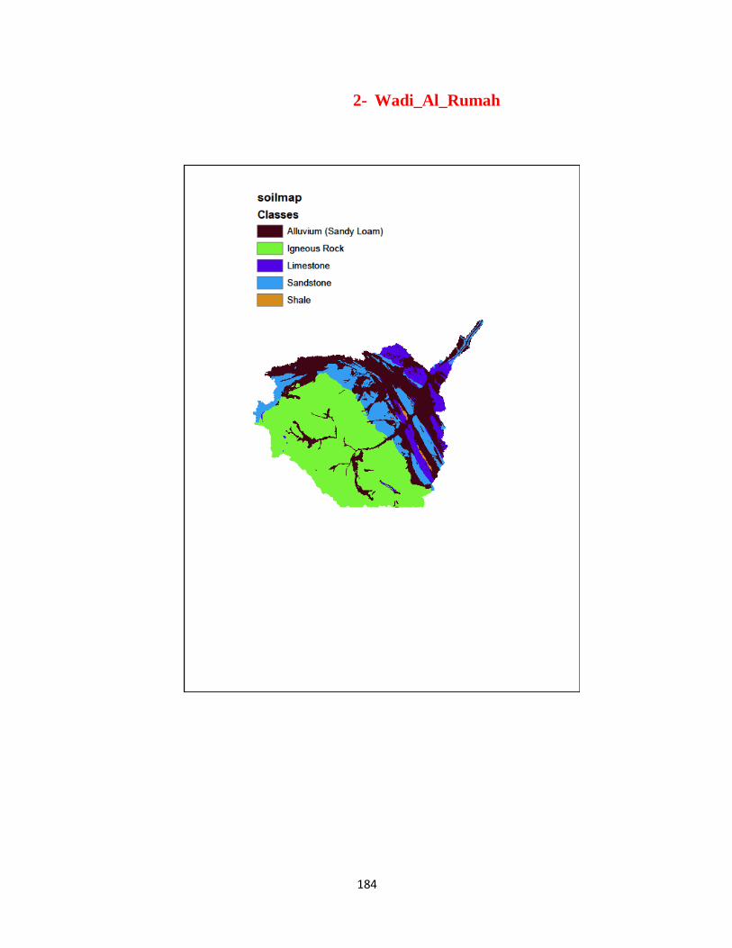
184
2- Wadi_Al_Rumah
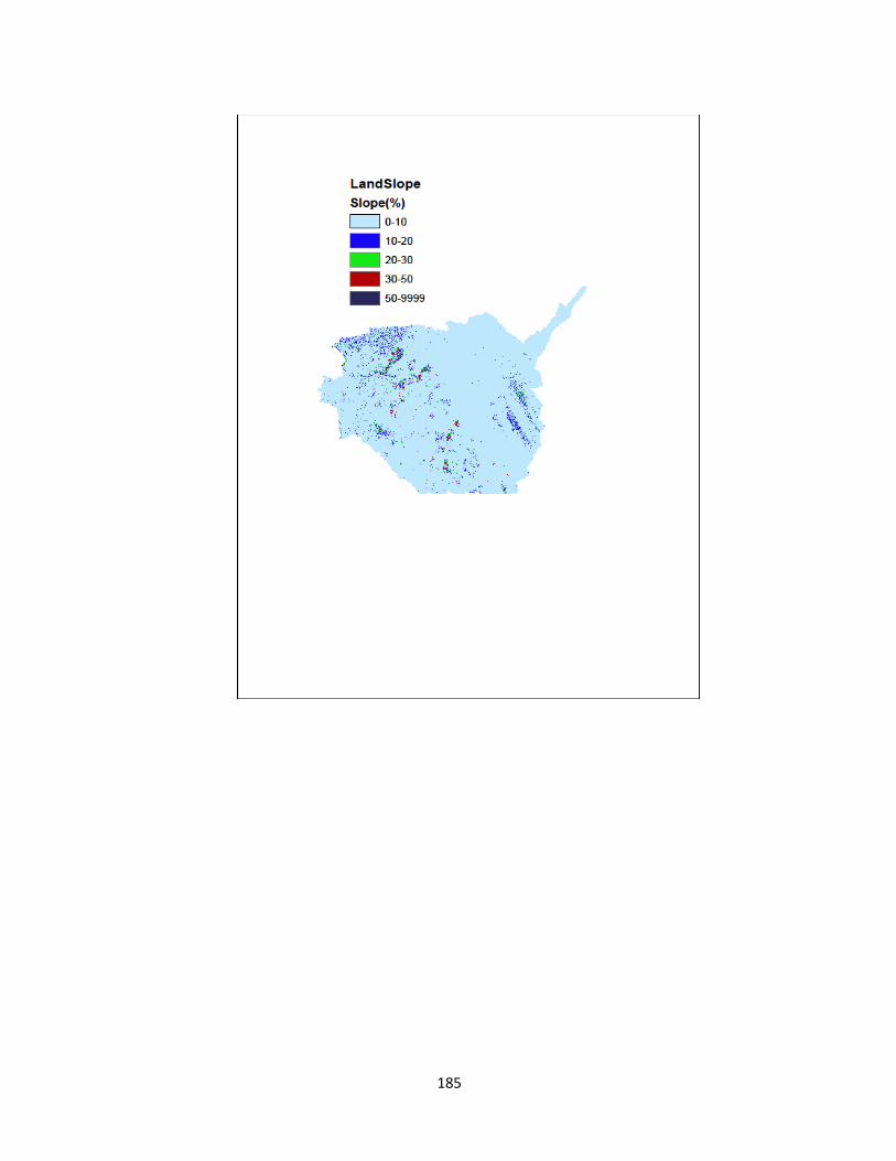
185
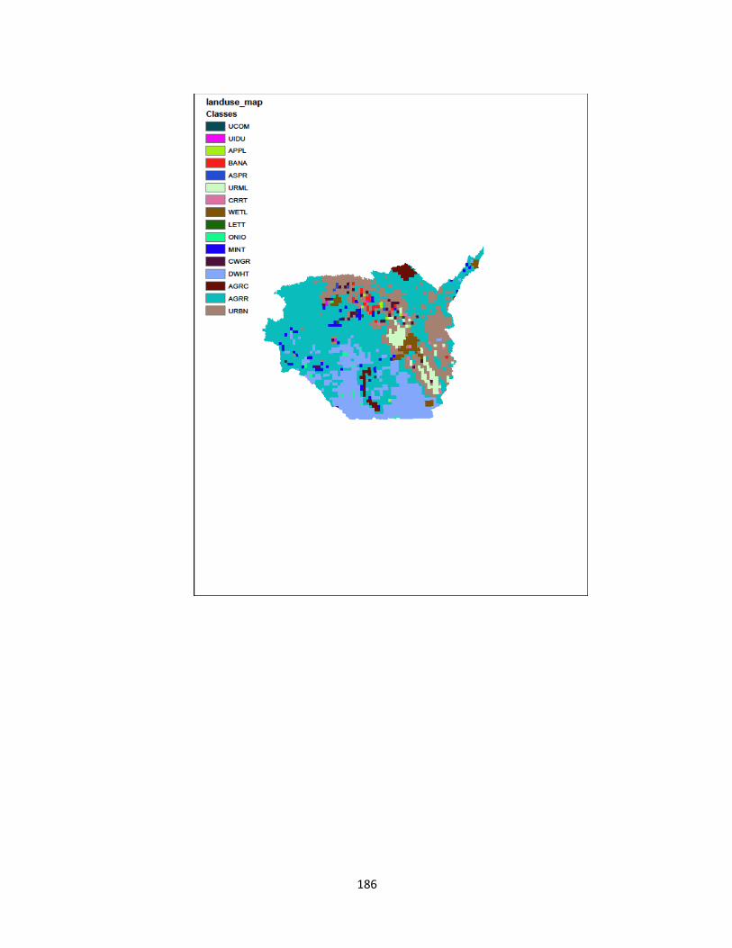
186
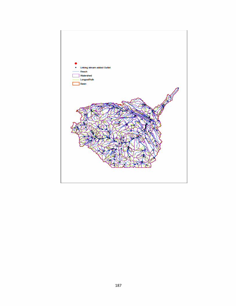
187
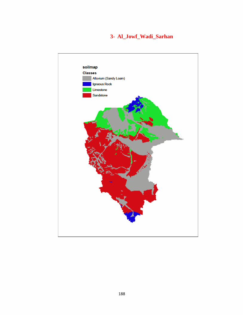
188
3- Al_Jowf_Wadi_Sarhan
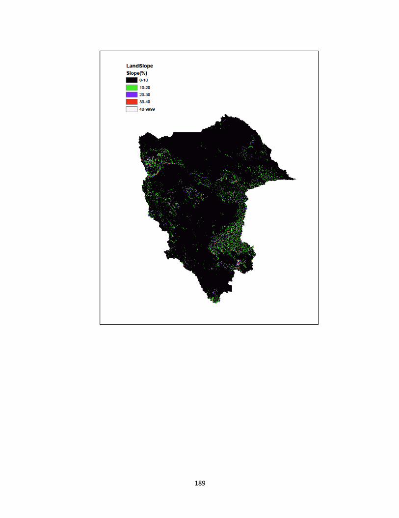
189
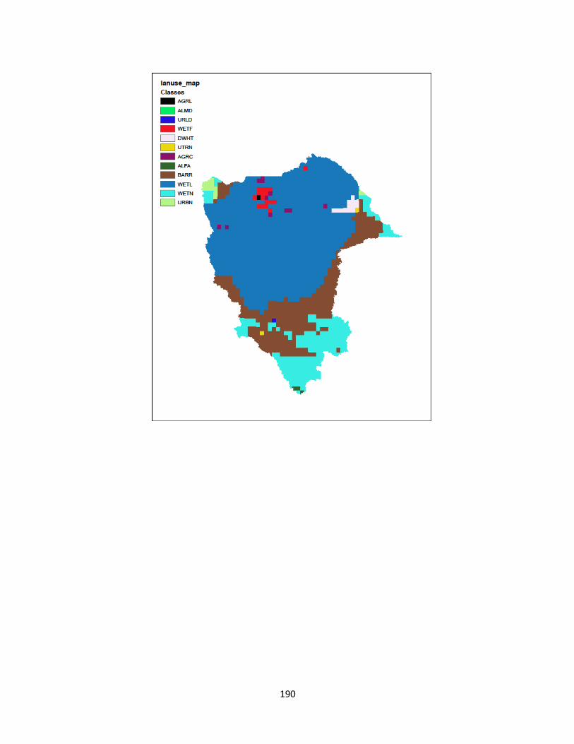
190
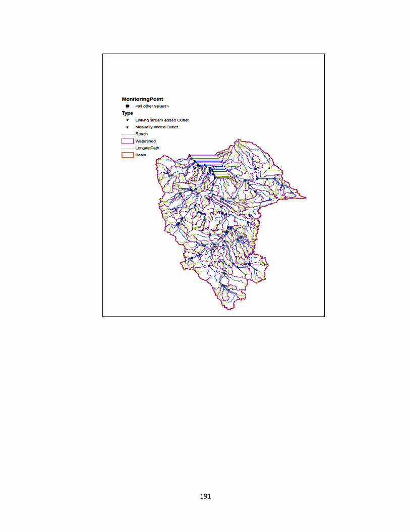
191
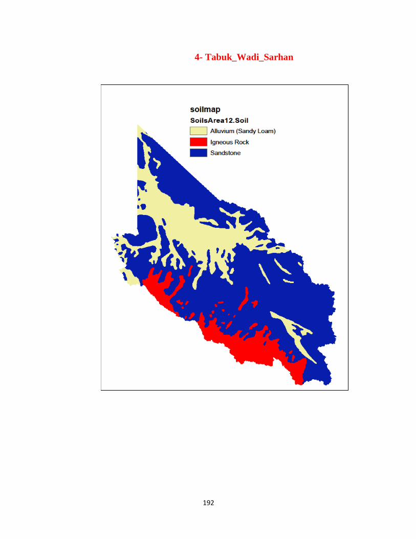
192
4- Tabuk_Wadi_Sarhan
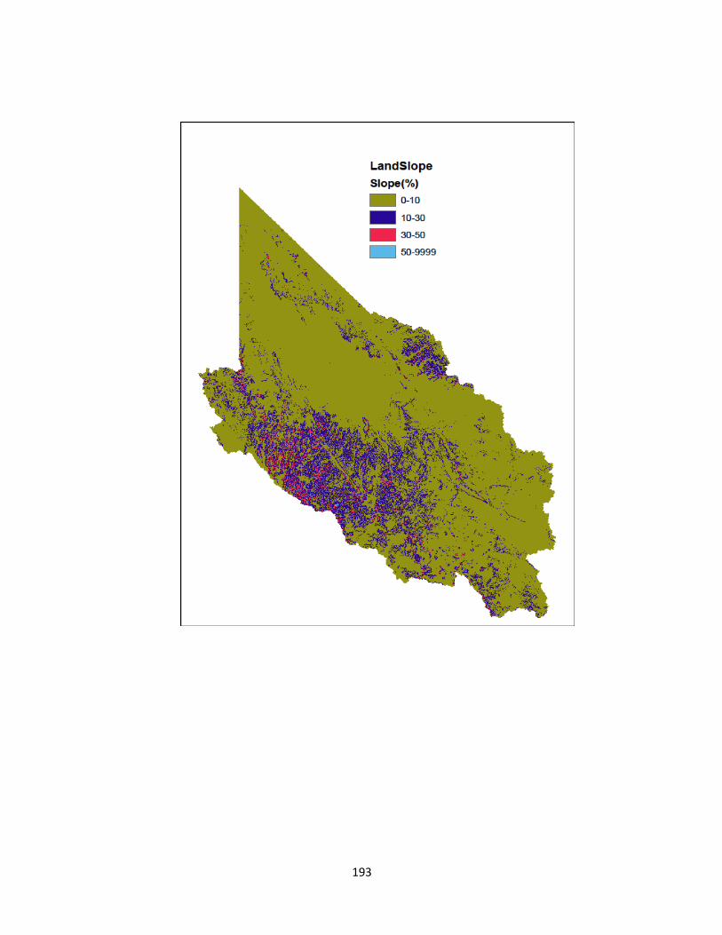
193

194
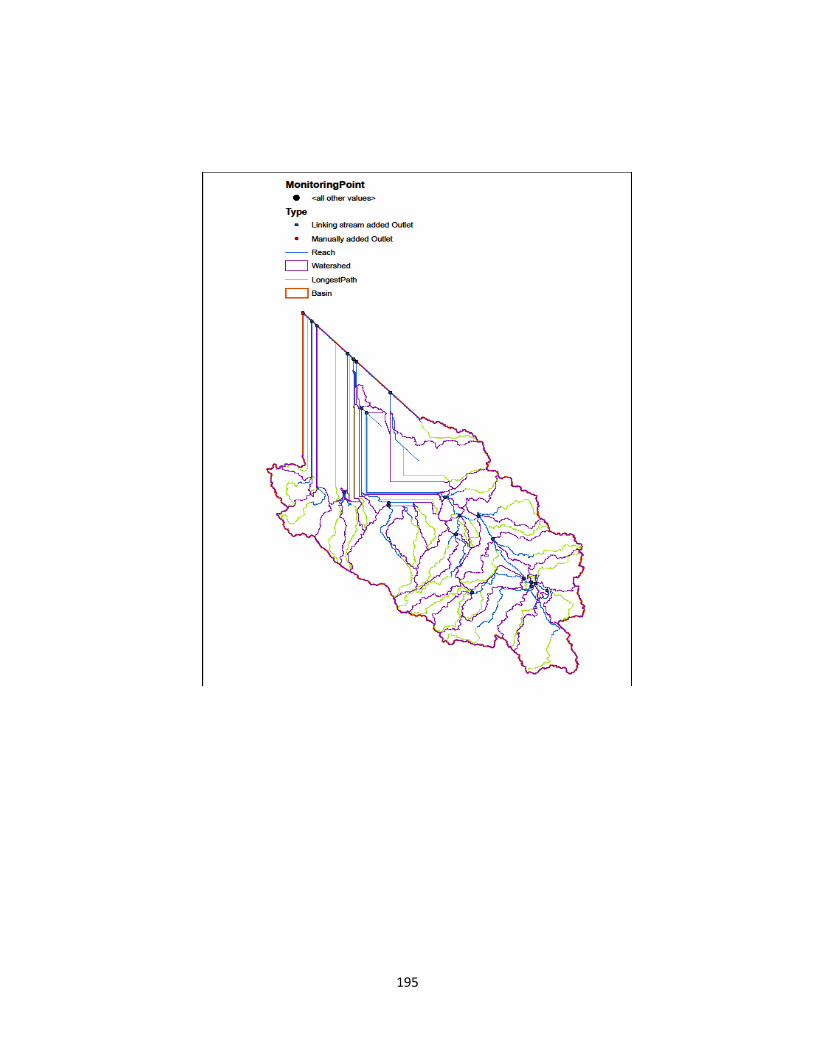
195