assessing energy price induced improvements in efficiency of capital in oecd manufacturing...

Contents lists available at ScienceDirect

Journal ofEnvironmental Economics and Management

Journal of Environmental Economics and Management 68 (2014) 340–356

http://d0095-06

n CorrE-m

journal homepage: www.elsevier.com/locate/jeem

Assessing energy price induced improvements in efficiencyof capital in OECD manufacturing industries

Jevgenijs Steinbuks a,n, Karsten Neuhoff b

a Development Research Group, The World Bank, MC-3-333, 1818 H St. NW, Washington, DC 20433, United Statesb Department of Climate Policy, DIW Berlin, Germany

a r t i c l e i n f o

Article history:Received 8 April 2013Available online 5 August 2014

JEL classification:D24E22Q41Q43

Keywords:Energy efficiencyEnergy pricesInvestmentVintage capital

x.doi.org/10.1016/j.jeem.2014.07.00396/& 2014 Elsevier Inc. All rights reserved.

esponding author.ail addresses: [email protected] (J. S

a b s t r a c t

To assess how capital stocks adapt to energy price changes, it is necessary to account forthe impacts on different vintages of capital and to account separately for price-inducedand autonomous improvements in the energy efficiency of capital stock. The results ofeconometric analysis for five manufacturing industries in 19 OECD countries between1990 and 2005 indicate that higher energy prices resulted in smaller energy use due toboth improved energy efficiency of capital stock and reduced demand for the energyinput. The investment response to energy prices varied considerably across manufacturingindustries, being more significant in energy-intensive sectors. The results of policy simula-tions indicate that a carbon tax can deliver significant reductions in energy consumption inthe medium run with modest declines in energy-using capital stock.

& 2014 Elsevier Inc. All rights reserved.

Introduction

Empirical analysis of the effect of energy prices on manufacturing input use has been so far limited by the ability ofeconometric models to reflect the adaptation of the capital stock to energy price changes. Griffin and Schulman (2005, p. 5)describe the problem as follows: “In a properly specified econometric demand model, the stocks of energy-using equipmentwould be modeled with a number of investment and depreciation equations for each type of energy using capital. Energyconsumption would then depend on the utilization and efficiency characteristics of the stock of equipment. Such anelaborate model could then be simulated to describe the adaptation of the capital stock to energy price shocks. But giventhe absence of capital stock data needed to reflect the adjustment of the capital stock of energy using equipment,econometricians estimate reduced form single demand equations featuring a distributed lag on price to capture theadaptation of the capital stock.”

While reduced-form econometric models of energy demand are useful in a number of respects, they fail in answeringsome important questions. First, though these models make it possible to obtain and compare short-run and long-runelasticities, they do not describe the path to the long run, or the pattern of investment in energy-using capital stock overtime (Pindyck and Rotemberg, 1983). Second, these models can say very little about the sources of changes in energydemand and energy efficiency (or its reciprocal – energy intensity). Finally, it is difficult to reconcile the conclusions fromreduced-form models aiming to study the short-run disequilibria associated with the incomplete adjustment of the capital

teinbuks), [email protected] (K. Neuhoff).

www.sciencedirect.com/science/journal/00950696

www.elsevier.com/locate/jeem

http://dx.doi.org/10.1016/j.jeem.2014.07.003



http://crossmark.crossref.org/dialog/?doi=10.1016/j.jeem.2014.07.003&domain=pdf



mailto:[email protected]

mailto:[email protected]


J. Steinbuks, K. Neuhoff / Journal of Environmental Economics and Management 68 (2014) 340–356 341

stock and the long-run equilibria in which the capital stock turns over completely. As Griffin and Schulman (2005, p. 5) pointout, “trying to do both with such a simple model may accomplish neither objective.”

This paper attempts to address this important limitation. Drawing from earlier works by Fuss (1977), Berndt et al. (1981),Atkeson and Kehoe (1999), Popp (2001), Sue Wing (2008), and, especially, Pindyck and Rotemberg (1983), we set up astructural, dynamic, and intertemporally consistent econometric model, which explicitly incorporates the capital stock, andseparately accounts for the transitional dynamics of capital due to the changes in input prices and autonomous capitalefficiency improvements. Specifically, we expand the traditional estimation of energy, materials, and labor responses toinput price changes by including vintages for the capital stock.1 Each vintage of the capital stock has its own energyefficiency, which is a function of input prices at the time of investment, and exogenous technological change. As with mostnew model developments, introducing capital vintages is costly; to make the model estimable we have to assume that theservices of assets of different vintages are perfect substitutes, and these assets depreciate geometrically at a constant rate.Under those assumptions we can represent the efficiency of the capital stock with a single index, weighted by the relativeefficiencies of the past vintages of capital.2 Adding vintage structure captures the adaptation of capital stock to energyprices, while preserving the flexibility of substitution between input factors to production (labor, energy and materials).

Our paper is relevant to several recent studies aimed at understanding determinants of energy efficiency improvements.Perhaps the most closely related paper is Koopmans and te Velde (2001), who also develop a vintage capital model of energydemand, in which the efficiency of energy-using capital stocks responds endogenously to energy prices. Unlike our paper,Koopmans and te Velde (2001) do not structurally estimate the parameters of their model. Instead they calibrate their modelbased on a large bottom-up database for the economy of the Netherlands, and then solve it numerically. They find that theaverage pace at which new energy-efficient technologies become available varies across time, thus elucidating the key weaknessof the bottom-up modeling approach, which relies on extrapolation of historical trends of energy efficiency improvements.Metcalf (2008) adapts an index number based theoretical approach, and finds that roughly three-quarters of the improvementsin the U.S. energy intensity since 1970 results from efficiency improvements due to the rising energy prices and per-capitaincome. Sue Wing (2008) estimates a structural model, which attributes most of the changes in the U.S. energy intensity toadjustments of quasi-fixed inputs and disembodied autonomous technological progress. The study concludes that “price-inducedsubstitution of variable inputs generated transitory energy savings, while innovation induced by energy prices had only a minorimpact.” (Sue Wing, 2008, p. 21). However, neither of the studies investigated the significance of price-induced improvements inthe energy efficiency of capital stock.

The distinction between energy price-induced and autonomous changes in efficiency of capital stock presented in this paper isimportant for both researchers and policy makers, especially in the context of climate change mitigation. The ease of adjusting thecapital stock is a critical determinant of the short-run transition costs of a energy and climate policies. The choice of input efficiencymade at the time of investment has long-term implications. An energy-inefficient and capital-intensive power plant ormanufacturing belt typically stays in production for many years before it retires from the production process. Upgrades toachieve better energy efficiency are not always technologically feasible or might be too costly to implement. Jacoby andSueWing (1999, p. 73) argue that “each year of delay [to implementing climate policies] introduces more emission-producingactivities that must be squeezed out of the system and shortens the time horizon for change, raising the carbon price requiredto produce the needed changes in capital structure.” And the costs and benefits of choosing technologies with better energyefficiency vary across manufacturing industries. For example, assuming the same installation costs, the net benefits frominstalling (more expensive) energy efficient technology will be larger for more energy-intensive (e.g. petrochemical, steel)industries. Understanding firms' investment response to energy prices provides guidance for decarbonization trajectories.3

Market-based climate policies aimed at reduction in fossil fuel consumption will succeed if firms' investment is responsive toenergy prices.

Our model is estimated for five manufacturing industries in 19 OECD countries between 1990 and 2005 using a restrictedvariable cost function approach. Compared to earlier models our cost-share equations are non-linear in factor prices because ofthe composite effect of input substitution and changes in the efficiency of capital stock. This introduces additional complexity forthe estimation of the relevant parameters of the model, and provides a better explanation of energy demand at the sector level.The assumption of constant efficiency of capital stock is rejected for all sectors.

1 The idea of using vintage capital in economic analysis dates back to Johansen (1959), who introduced this concept in the context of deterministicgrowth model. Other notable contributions investigating different properties of vintage capital include Solow et al. (1966), Sheshinski (1967), Malcomson(1975), Fuss (1977), and, more recently, Chari and Hopenhayn (1991), Benhabib and Rusticini (1991), and Boucekkine et al. (1997). In the energy andenvironmental economics literature, vintage capital models have been intensively used mainly in the context of understanding the properties of embodiedenergy-saving technological progress. Recent contributions include Meijers (1994), Mulder et al. (2003), Hart (2004), Pérez-Barahona and Zou (2006), andAzomahou et al. (2012).

2 In this regard our econometric approach is similar to Haas and Schipper (1998) and Koopmans and te Velde (2001), who advocate calculating anindex of energy efficiency, and using it directly in econometric specification for energy demand. The index of Haas and Schipper (1998) though is obtainedthrough factor decomposition, and is thus purely exogenous.

3 Many computational economic models of energy climate change (e.g. U.S. EIA NEMS Industrial Demand Module, OECD ENV-Linkages model, and MITIntegrated Global System Modeling framework) employ capital vintage structure. Validation of energy price response vintage elasticities in these modelsbased on rigorous econometric analysis (attempted in this study) remains an important problem to be solved. The authors thank John Reilly for makingthis point.

J. Steinbuks, K. Neuhoff / Journal of Environmental Economics and Management 68 (2014) 340–356342

The results for all industries indicate that energy prices result in smaller energy use due to both improved energyefficiency of capital stock and reduced demand for energy input. Estimated own-price elasticities of energy demand vary inthe range of 0.21 and 0.86, and are in line with the previous estimates. Estimated elasticities of energy input efficiency withrespect to energy price vary between 0.015 (electrical and optical equipment industry) and 1.1 (for petrochemical industry).The investment response to energy prices thus varies considerably across manufacturing industries, being more significantin energy-intensive industries. We also find substantial autonomous improvements in the energy efficiency of capital stockover recent decades, ranging between 2 and 4 percent per annum. These results indicate that differences in the estimatedinvestment response to energy prices from the previous empirical studies can be, to some extent, attributed to theaggregation problem.

An important finding of this paper is that energy and climate policies aimed at reductions in fossil fuel emissions canresult in substantial reductions in energy use in energy intensive sectors. To illustrate this point we conduct a counterfactualanalysis of an increase in energy prices due to a $30/ton greenhouse gas emissions tax for the U.K. petrochemical andelectrical industries (i.e., the most and the least energy-intensive industries in the sample). The results of this analysisindicate that an increase in energy prices results in a considerable decline in energy use. The combined (i.e., operational andinvestment) own-price elasticity of energy demand is between 0.7 and 0.8. At the same time, the reductions in capital stockin the medium-run are negligible. In the petrochemical industry, the decline in capital stock resulting from short-runenergy-capital complementarity is offset by increasing the demand for more energy-efficient capital. In the electricalindustry energy using capital stocks is little changed because of weak complementarity between energy and capital.

The rest of this paper is structured as follows. The second section outlines the vintage capital model and resultingstochastic specification. The third section describes the dataset. The fourth section presents the main findings of theresearch. The fifth section discusses the modeling assumptions. The sixth section presents the results of policy simulations.The final section concludes, and suggests policy recommendations.

Vintage capital model of energy/demand

We introduce a dynamic partial equilibrium model that separately accounts for investment and operational (production)decisions in the manufacturing sector. The model allows for adaptation of the capital stock in response to energy priceshocks and contributes to existing literature on modeling input demands, by providing a unified empirical framework forsubstitution between input factors of production (labor, energy and materials), and the potential for more efficient useof these inputs by choosing more efficient technologies at the time of investment. The model focuses on production andinvestment decisions over the short and the medium run. Firms choose between different types of capital from an existingportfolio of available technologies, which improve gradually over time. The research and development, and capital-goodsproducing sectors that account for long-run response to energy prices by extending the range of available technologies(Popp, 2002) are not considered in this partial equilibrium model of manufacturing decisions.

We start with the firms' investment. Forward-looking firms add newmanufacturing assets based on a specific productiontechnology. Following the economic literature of capital measurement (Diewert, 1980; Jorgenson, 1980; Jorgenson et al.,1987), we can refer to these manufacturing assets acquired at different points in time as different vintages of capital. Foreach capital vintage, firms choose the optimal level of input efficiency of production technology, given autonomousefficiency improvements (Webster et al., 2008) and their expectations of future input costs.

Once the investment is made, the new energy-using capital stock remains to be operational until it depreciates away or isreplaced. The replacement of existing capital stock is, however, costly in the short run. Our vintage capital model thus fits inthe framework introduced by Fuss (1977), in which the substitution of factors of production is easier ex ante than ex post. Animportant characteristic of such a framework, as noted by Koopmans and te Velde (2001, p. 58), is that “following anunexpected energy price increase, the energy efficiency of new vintages will improve more than the energy efficiency ofexisting vintages. A price change achieves its full impact only after the capital stock has been completely renewed. Hence,price elasticities are larger in the long run than in the short run.” In the extreme case of infinitely large capital adjustmentcosts our model becomes similar to the Atkeson and Kehoe (1999) “putty-clay” model of energy use.

We then consider production decisions based on the dynamic factor demand model of Pindyck and Rotemberg (1983),where firms minimize expected input costs (including capital adjustment costs) to produce the optimal time path of labor,capital, energy, and materials consumption to achieve the desired output level, given the level of input efficiency of installedproduction technology. The resulting equations are subsequently used to form stochastic specifications and estimate theinput price elasticities of factor substitution and capital stock efficiency.

Investment in input efficiency

We assume that the manufacturing industries in OECD countries operate in perfectly competitive product and factormarkets, that is, take input prices as given. We can therefore view each manufacturing sector as consisting of a single firmthat has certain production technology, or, equivalently, as consisting of many firms whose aggregate technology isrepresented by our model (Pindyck and Rotemberg, 1983). At any time t the firm i is fully flexible in its choice of labor ðxli;tÞ,energy ðxei;tÞ, and materials' ðxmi;tÞ inputs. The capital stock ðxki;tÞ is quasi-fixed (i.e., fixed in the short run, and flexible in thelong run), and has vintage representation. Each vintage of capital stock has its own technological efficiency with respect to


other inputs to the production function. The investment in factor efficiency of a capital vintage is sunk, i.e., the productiontechnology is inflexible in terms of the capital efficiency requirements. We assume that the services of assets of differentvintages are perfect substitutes, and these assets depreciate geometrically at constant rate δ. Under those assumptionsJorgenson et al. (1987, pp. 4049) have shown that the flow of capital services is a weighted sum of past investments, with theweights corresponding to the relative efficiencies of the different vintages of capital. Investment in a capital vintage inperiod q can then be inferred from the following equation:

Ii;q ¼ xki;q�ð1�δÞxki;q�1: ð1Þ

We assume that in any period q the efficiency of a vintage of capital stock, xki;q, with respect to other inputs, labor, xli;q, energy,ðxei;qÞ, and materials, ðxmi;qÞ, is represented by an index γji;q, where j¼ l; e;m. The index γji;q measures the amount of labor, energy andmaterials' inputs required to produce the input service, i.e., output of useful work (however measured).4 While firms maketechnology choices in period q, there is a lag between the firm's investment decision and the plant commissioning. The technologyis installed and becomes fully functional in period qþ1. Firms' production decisions in period q are thus made based on theproduction technology installed in period q�1.

The quantity of input j¼ l; e;m in period q, xji;q, and the index of input efficiency of capital vintage, γji;q�1, determine theinput service to the production function, ~xji;q:

~xji;q ¼xji;qγji;q�1

; γji;q40; ð2Þ

Similarly, the relationship between the price of the input in period q, wji;q and the price of service ~wj

i;q is given by

~wji;q ¼wj

i;qγji;q�1: ð3Þ

Eqs. (2) and (3) imply that the lower the value of the index of the input efficiency of capital vintage, γji;q�1, is, the moreservices the capital vintage xki;q can produce from a given input j¼ l; e;m, and the lower the price of that service is. As thevintage of capital stock cannot produce more services with respect to itself, we assume that the value of the index of capitalefficiency of capital stock is equal to one for all capital vintages:

γki;t ¼ 1: ð4Þ

The input efficiency of capital vintage q that firms choose to produce a flow of services from energy, labor, and materialsis determined endogenously based on the input prices and the exogenous technological change5:

γji;q ¼ ð1�ζÞqwj

i;q

wj

!�ϕj

; j¼ l; e;m; ð5Þ

where w is the average price of input j across countries and all time periods,6 ϕj is the elasticity of the efficiency of input jwith respect to input price changes, and ζ is the rate of exogenous Hicks-neutral technological change.7 In the OnlineAppendix (Section A.1) we show that this equation is consistent with the profit maximization (cost minimization) of aforward-looking firm that faces a technology cost function.

Let z be the first capital vintage observable to an econometrician. Then, for all observed capital vintages qZz we canderive the index of input efficiency of capital stock γji;t as a sum of historic vintage efficiencies weighted by each vintage's qcontribution to capital stock xkt :

γji;t ¼ ∑t

q ¼ zð1�ζÞq

wji;q

wj

!�ϕj

Ii;qð1�δÞt�q

xki;t; j¼ l; e;m; ð6Þ

where Ii;q is the vintage investment in period q, and δ is the rate of economic depreciation of capital stock.8

Because we do not know the values of the index of input efficiency of capital stock for vintages outside the observedsample, we assume that they are the same as in the first period of the observed sample. Under this assumption the index of

4 For example, if average internal temperature is taken as the appropriate measure of useful work from manufacturing heating system, labor efficiencyof capital stock will depend on the degree of thermal system's automation, energy efficiency of capital stock will depend upon the thermal efficiency of theboiler, whereas materials' efficiency of capital stock will depend upon the quality of thermal insulation.

5 As we explained earlier our model focuses on medium-term investment decisions, where firms choose between different types of capital from anexisting portfolio of available technologies. Exogenous technological change here captures the fact that available technologies improve gradually over time.

6 We have chosen the OECD average input price across countries and all time periods to reflect the effects of globalization and industry migration. Wealso considered the input price based on the country average across time: wj

i ¼∑Tt ¼ 1w

ji;t=T . Estimation results were not different.

7 In the next section we also allow for non-neutral disembodied technological change in firms' operational choice problem.8 Interpretation of the index of input efficiency of capital stock becomes difficult if vintage investment is negative. Almost all observations in our

dataset corresponded to positive vintage investment. To avoid confusion with interpretation of the index of input efficiency of capital stock, we set its valueequal to the previous period in rare cases of negative vintage investment.


input efficiency of capital stock with respect to energy, labor and materials for all observations becomes

γji;t ¼ ð1�δÞtxki;0

xki;t

wji;0

wj

!�ϕj

þ ∑t

q ¼ 1ð1�ζÞq

wji;q

wj

!�ϕj

Ii;qð1�δÞt�q

xki;t; j¼ l; e;m; ð7Þ

where the first term on the right-hand side is the value of the index of input efficiency of capital stock in the first period ofthe observed sample.9

Input demand

Derivation of the operational choice of input factors is based on the dynamic factor demand model of Pindyck and Rotemberg(1983). We assume that the production technology is represented by a restricted variable cost function. Conditional on realization ofcapital stock, xki;t , and output Yi;t at time t, the minimum real expenditure on labor, energy, and materials is given by a functionCð ~wl

i;t ; ~wei;t ; ~w

mi;t ; x

ki;t ;Yi;t ; tÞ. The function C is assumed to be increasing and concave in input prices of labor, energy, and materials,

and decreasing and convex in capital stock. The changes in capital stock are subject to adjustment costs, represented by a convexfunction, cðItÞ.

Factor demands are given by the solution to the following dynamic optimization problem:

min~wl ; ~we ; ~wm ;xk

E ∑T

t ¼ τRt ½Cð ~wl

i;t ; ~wei;t ; ~w

mi;t ; x

ki;t ;Yi;t ; tÞþwk

i;txki;tþcðItÞ�; ð8Þ

subject to Eq. (1), where E denotes the expectational operator, and Rt is the discount rate for revenues accumulating at timet. The expectation operator in the objective function (8) applies to the future values of ~wl

i;t ; ~wei;t ; ~w

mi;t and Yi:t , which are

treated as random. Differentiating the objective function (8) with respect to choice variables ~wl; ~we; ~wm, and xk yields thefollowing equations:

∂Ci;t

∂ ~wji;t

¼ ~xji;t ; j¼ l; e;m; ð9Þ

∂Ci;t

∂xki;tþwk

i;tþ∂cðxki;t�ð1�δÞxki;t�1Þ

∂xki;tþE Rt

∂cðxki;tþ1�ð1�δÞxki;tÞ∂xki;t

" #¼ 0; ð10Þ

and

limt-1

E Rt∂Ci;t

∂xki;tþwk

i;tþ∂cðxki;t�ð1�δÞxki;t�1Þ

∂xki;t

" #( )¼ 0: ð11Þ

Eq. (9) is the standard result of Shephard's Lemma. Eq. (10) is the Euler equation, which describes the (expected) evolution of thequasi-fixed capital stock. Eq. (11) is the transversality condition, which ensures that the quantity capital that firms expect to hold isnot very much different from the quantities they would hold in the absence of adjustment costs.

Specification and estimation of the vintage capital model

Before estimating the vintage capital model we must specify the functional forms of the expenditure function, C, and theadjustment cost function, cðIÞ. Following Pindyck and Rotemberg (1983), we assume that the restricted variable cost functioncan be approximated by the translog model:

log Ci;t ¼ α0þ∑jαij log ~wj

i;tþαiK log xki;tþαiY log Yi;tþαiτt

þ12∑j∑pβjk log ~wj

i;t log ~wji;tþ∑

pβjK log ~wj

i;t log xki;t

þ∑jβjY log ~wj

i;t log Yi;tþ∑jβjτ log ~wj

i;t t

þβKY log xki;t log Yi;tþβKτ log xki;t tþβYτ log Yi;t t

þ12βKKðlog xki;tÞ2þ

12βYY ðlog Yi;tÞ2þ

12βττt

2; j; p¼ l; e;m: ð12Þ

9 We attempted to estimate the joint efficiency of all unobserved capital stock vintages as a free parameter, but were unable to obtain estimates ofreasonable magnitude because of flatness in the estimated non-linear likelihood function. Estimates of other parameters did not change significantly ineither signs or magnitudes after imposing this restriction.


We add the time trend, t, in Eq. (12) to allow for factor-specific disembodied technological progress. The adjustment costfunction for capital stock is assumed to be quadratic, that is

cðIi;tÞ ¼ λI2i;t=2: ð13Þ

With this specification, Eqs. (9) and (10) become

Sji;t ¼ αijþβjK log xki;tþβjY log Yi;tþβjτtþ∑jβj log ~wj

i;t ; j¼ l; e;m; ð14Þ

and

Ci;tSKi;t=x

ki;tþwk

i;tþλðxki;t�ð1�δÞxki;t�1Þ�EfRtð1�δÞλ½xki;tþ1�ð1�δÞxki;t �g ¼ 0; ð15Þ

where

Sji;t ¼∂ log Ci;t

∂ log ~wji;t

¼~wji;t~xji;t

C¼wj

i;txji;t

C; j¼ l; e;m; ð16Þ

is the share of each input j in firms' total variable cost, and SKi;t is defined as

SKi;t ¼ αiK þβKK log xki;tþβKY log Yi;tþβKτtþ∑jβjK log ~wj

i;t : ð17Þ

Combining Eqs. (3), (7), (14), and (15) yields the system of equations to be estimated. Model estimation is confounded byseveral econometric issues, which require additional clarification. First, we assume that deviations of fitted cost shareEqs. (14) and (15) from the logarithmic derivatives of the translog cost function (12) are the result of random errors in costminimizing behavior. We append to Eqs. (14) and (15) an additive disturbance term, εijt , which is independently andidentically normally distributed with mean vector zero and nonsingular covariance matrix Ω. This assumption implies thatthe supply of inputs is perfectly elastic, and therefore that input prices can be taken as exogenous (Berndt and Wood, 1975,p. 261). However, input prices and quantities could be endogenous at the individual industry level, and render the estimatedcoefficients to be biased and inconsistent. To account for this endogeneity problemwe use average estimates for input pricesin the entire manufacturing sector.10 An alternative approach of instrumental variables estimation appears to beproblematic primarily because of large measurement errors in energy prices at the individual industry level (see sectionbelow), and also because of the general difficulty of finding good instruments (Diewert and Fox, 2008). As demonstrated bya number of studies (Griffin and Gregory, 1976; Barnett et al., 1991; Burnside, 1996), the small sample bias from a set ofpopular instrumental variables (lagged prices, population, taxes, government purchases) is not necessarily smaller than thatobtained from actual prices.

Second, estimation of the Euler equation (15) would yield biased and inconsistent parameter estimates if there is acorrelation between the actual variables at time t and the expected value of capital stock in period tþ1. To account for thisproblem we estimate the model in two stages. In the first stage we employ dynamic panel data estimation techniques(Arellano and Bover, 1995; Blundell and Bond, 1998) to instrument for the capital stock using lagged input prices and outputas instruments. In the second stage we estimate the model using instrumented capital stock in lieu of actual capital stock.

Third, the system of equations to be estimated is a non-linear problem, where the parameters ϕj and ζ should beevaluated at each data point across the time-series dimension. This makes traditional estimation approaches, such as e.g.,iterated feasible generalized non-linear least squares (IFGNLS), non-applicable as they exhaust the degrees of freedomin panels with short individual dimension N. Instead, following Popp (2001) and Sue Wing (2008), we treat the system ofequations as a conditionally linear problem. Conditional on realization of unknown parameters ϕj and ζ, the system ofequations becomes a seemingly unrelated regression, which is efficiently estimated by full information maximum likelihood(FIML).

The values of parameters ζ and ϕj are chosen to maximize the value of the model's goodness-of-fit criterion, and areobtained by a multidimensional stochastic grid search (Judd, 1998, p. 296). To minimize the computational burden ofa multidimensional grid search, based on the earlier empirical findings (e.g., Jorgenson and Fraumeni, 1981; Baltagi andGriffin, 1988; Newell et al., 1999; Sue Wing, 2008; Webster et al., 2008) we set the estimation bounds for the exogenoustechnological change parameter, ζ, to vary between �0.03 and 0.05, and the elasticity of input efficiency of capital stockwith respect to input price changes, ϕj, between 0 and 1.5.11 Because the cost share equations in the system of Eqs. (14) addto one, only two share equations are estimated.

While the system of Eqs. (3), (7), (14) and (15) forms our basic empirical model we also estimate a restricted model,assuming that the input efficiency of capital stock does not change, so γji;t is set to 1 (or both ζ and ϕj are set to zero). Under

10 Endogeneity problem remains if total output of a manufacturing industry affects input prices, and output is correlated across manufacturingindustries. This is highly unlikely for any country in the sample, including the U.S.

11 We have examined the model sensitivity to relaxing the range of estimation bounds, and the results turned out to be robust (no corner solutions).


this restriction the model becomes the dynamic factor demand model of Pindyck and Rotemberg (1983). We then use thelikelihood-ratio test to evaluate the significance of the input efficiencies of capital stock in the models of energy demand.

To quantify the operational response to current price changes holding all previous prices constant, we compute own-price and cross-price elasticities of substitution,12 as well as the elasticities of flexible input demand with respect to changesin output and capital stock.13 These elasticities are given by

ηjj ¼∂ ln xji;t∂ ln wj

i;t

¼βjjþðSji;tÞ2�Sji;t

Sji;t; j¼ l; e;m: ð18Þ

ηpj ¼∂ ln xji;t∂ ln wp

i;t

¼βpjþSpi;tS

ji;t

Sji;t; p; j¼ l; e;m; pa j: ð19Þ

ηjK ¼∂ ln xji;t∂ ln xki;t

¼ βjK

Sji;tþαiK þβKK log xki;t

� �þ∑

pβpK log ~wj

i;t ; p; j¼ l; e;m: ð20Þ

and

ηjY ¼∂ ln xji;t∂ ln Yi;t

¼ βjY

Sji;tþαiY þβYY log Yi;t

� �þ∑pβpY log ~wj

i;t ; p; j¼ l; e;m: ð21Þ

Estimated elasticities have a standard economic interpretation and capture several separate substitution effects,including within-firm input substitution and within-industry compositional changes.14 Because we include country-specific fixed effects, and identify coefficients, β, based on the within-country variation over time, the operational responseelasticities, ηjj, and, ηpj, capture short-run equilibrium effects. On the contrary, the investment elasticities of input efficiencyof capital stock with respect to input price changes, ϕj, and exogenous technological change, ζ, incorporate the dynamics ofthe capital stock and capture medium- and long-run equilibrium effects.

Data

The vintage capital model is estimated using panel data from 19 OECD countries between 1990 and 2005 separately for fivemanufacturing industries – food, beverages and tobacco (ISIC sectors 15 and 16); pulp, paper products, paper, and publishing(ISIC sectors 21 and 22); chemical, rubber, plastics, and fuel products (ISIC sectors 23, 24, and 25); basic metals, and fabricatedmetal products (ISIC sectors 27 and 28); and electrical and optical equipment (ISIC sectors 30, 31, 32, and 33).15 The use ofdisaggregated data reduces the measurement error and improves the quality of the estimates, as different sectors use energy fordifferent purposes, which affects their ability to substitute between energy and other inputs.16 Due to data limitations on capitalstocks the analysis was not possible for other sectors as well as at a less aggregate level.

The main data source for empirical analysis is the EU KLEMS database, which is constructed based on the methodology ofJorgenson et al. (1987, 2005).17 The EU KLEMS database comprises data on production inputs, labor and capital input prices,18

and output at the industry level for the European Union, the United States, the Republic of Korea, and Japan. The relatively smallnumber of available observations makes it necessary to assume that each country's manufacturing industry has the sameproduction function. Though restrictive, this is a standard assumption made in inter-country studies of energy demand. To thebest of our knowledge there is no study addressing this issue, and doing so is beyond the scope of this paper. However, weexclude non-manufacturing industries (e.g., agriculture, commerce and transportation), where the assumptions of identicalproduction functions and rational cost minimizing firms are less likely to be satisfied.19 A full list of variables, countries and thedescriptive statistics for the final dataset are shown in Tables A.1–A.7 (Online Appendix, Section A.2).

Based on the estimates from Timmer et al. (2007, Appendix 1) we set economic depreciation rates at 11 percent in thefood processing industry, and 10 percent in all other industries. Because we do not have estimates for the rate for revenues

12 We have also estimated Allen's and Morishima's partial elasticities of substitution. Because these elasticities have less straightforward interpretation(Frondel, 2004), and can be directly inferred from estimated cross-price elasticities, their estimates are not reported.

13 To calculate these elasticities one needs the estimates of translog function (12), which is estimated separately.14 Sorting out between these effects is however beyond the scope of this paper.15 To preserve space in the text these industries are further referred to as food processing, pulp and paper products, petrochemical, metals, and

electrical industries.16 For example, manufacturing of steel and aluminum is based on high temperature heating and electrochemical processes that have few (if any)

available substitutes for energy. On the other hand, energy- and/or capital-intensive processes can be substituted for labor intensive processes in lightmanufacturing industries.

17 For more details, see Timmer et al. (2007) and O'Mahony and Timmer (2009).18 Data on the price of capital services were not available for some countries. For these countries following Andrikopoulos et al. (1989) and Cho et al.

(2004) we computed the capital input prices (available from IMF International Financial Statistics Database) as a sum of the nominal interest rate on short-term government papers, and the capital depreciation rate.

19 This is because manufacturing industries are globally interconnected, internationally competitive, less distorted by national policies, and have largecross-border flows of know-how. In a separate paper we estimate the vintage capital model for non-manufacturing industries.


accumulating at time t, Rt , we set it to 0.95. We performed sensitivity analysis assuming different values of Rt, and the resultswere not significantly different.

The EU KLEMS dataset does not include information on input prices for energy and materials. We use the International EnergyAgency (IEA) Energy Prices and Taxes database to extract the data on end-use prices for key fuels used in the OECD manufacturingindustries.20 We also use the IEAWorld Energy Statistics and Balances database to obtain industrial fuel consumption data. We thenconstruct the average energy price for the manufacturing sector by weighting energy carriers' prices by the consumption of eachenergy carrier in the manufacturing sector. To examine the robustness of our energy price calculations we calculate industrial fuelexpenditure using data from the IEA databases and compare it with industrial energy expenditure reported in the EU KLEMSdatabase. Correlation between the two series was close to 0.99 for the manufacturing sector aggregate. Unfortunately, thesecorrelations were considerably lower for individual industrial sectors, which indicates poorer correspondence between IEA and EUKLEMS at less aggregate levels. We therefore employ energy price data for the manufacturing sector aggregate.

We construct the price of materials by weighting international commodity prices (from the IMF International FinancialStatistics database) by sector consumption of each commodity (from the UNIDO Industrial production database). The dataseries for labor, energy, and material costs, and for the values of output and capital stock, are all deflated to their real valuesbased on the industry deflators, using 1995 as the base year, and converted into U.S. dollars at nominal exchange rates.21

Fig. 1 shows the average energy prices in the manufacturing sector across OECD countries in 2005. The highest energyprices are in Italy, Ireland, Japan and Sweden, and the lowest are in Australia, the Netherlands, Greece, and the United States.These differences in energy prices across OECD countries are because of variation in energy taxes, the types of fuels used inthe production process, and local distribution costs. Variation in industrial energy prices across the manufacturing industryin the OECD is relatively small compared to other sectors, such as commerce or transportation (International Energy Agency,2008). This may reflect constraints on national energy tax policies, which are major drivers of international energy pricedifferences,22 posed by countries' concerns to maintain their international competitiveness in the manufacturing sector(Brack et al., 2000).

Results of estimation of the vintage capital model

The empirical estimates of stochastic specification (3), (7), (14), and (15) applied separately to each of the five industriesover the period 1990–2005 across 19 OECD countries are presented in Tables A.8–A.12 (Online Appendix, Section A.2). Wepresent the results for both the vintage capital model, and the dynamic factor model of energy demand of Pindyck andRotemberg (1983), in which the indices of the input efficiency of capital stock are set to 1. Tables 1–3 present estimated own-price elasticities of input demand, cross-price elasticities of energy demand, and own-price elasticities of the input efficiency ofcapital stock from the vintage capital model. Tables A.13–A.17 (Online Appendix, Section A.2) demonstrate the variation ofestimated elasticities across countries. Estimated cross-price elasticities of other input demands are presented in Tables A.18and A.19 (Online Appendix, Section A.2). Figs. A.1–A.5 (Online Appendix, Section A.3) show the values of the calculated indicesof input efficiency of capital stock.

The regression results show that the vintage capital model generally provides a better explanation of energy demand. TheR-squared values are higher for the vintage capital model (Tables A.8–A.12, Online Appendix, Section A.2). The likelihood ratiotest indicates that the dynamic factor demand model restriction of input efficiencies of capital stock being equal to 1 is rejected atthe 1 percent level of significance for all five industry estimates.

Table 1 shows the estimated own-price elasticities of input demands across different countries and sectors. Theestimated elasticities have the expected sign, except in few countries, where input cost shares were close to zero (see TablesA.13–A.17, Online Appendix, Section A.2). This is a well-known problem documented in the previous studies using a translogmodel (Urga andWalters, 2003). However, in almost all cases, the elasticities were not statistically different from zero. Basedon the vintage capital model estimates, own-price elasticity of labor demand varies between �0.83 and �1.17, own-priceelasticity of energy demand varies between �0.21 and �0.86, and own-price elasticity of materials demand varies between�0.22 and �0.46. These results fall within the range of magnitudes of elasticities of the comprehensive survey of Barkeret al. (1995) and the estimates of more recent studies of energy demand in the OECD manufacturing sector. For example,energy demand elasticity estimates of Enevoldsen et al. (2007) range between �0.44 and �0.38 for 15 industrial sectors inNorway, Denmark, and Sweden. Agnolucci (2009) estimates a price elasticity of �0.64 for the German and British industrialsectors over the period 1978–2004. Adeyemi and Hunt (2007) model asymmetric energy demand response for 15 OECDcountries over the period 1962–2003, and find elasticities between �0.68 (price recoveries) and �0.30 (price cuts). Thevintage capital model and the dynamic factor demand model yield comparable estimates for labor and materials' demand,and different estimates for energy demand. The estimated own-price elasticities of energy demand based on the vintage

20 Specifically, we consider the following energy products – oil and petroleum products (high- and low-sulphur fuel oil, light fuel oil, automotive diesel,and gasoline), natural gas, coal, and electricity. Consumption of each product is measured in British thermal units (BTUs).

21 We have also estimated the model using dollar conversion at purchasing power parity exchange rates. The results were of comparable magnitude tothose reported below.

22 For example, in transportation sector international energy price differences are almost entirely due to gasoline tax, which accounts for nearly 60percent of final energy price in Sweden, Germany and the United Kingdom, compared to just 13 percent in the United States (International Energy Agency,2008).

Fig. 1. Average real energy prices in OECD manufacturing sector in 2005.

Table 1Own-Price Elasticities of Input Demand in OECD Manufacturing Sectors.

Sector ηll ηee ηmm

VCM P-R VCM P-R VCM P-R

Chemical, rubber, plastics and fuel products �0.91nnn �0.90nnn �0.21 �0.48n �0.43nnn �0.45nnn

(0.10) (0.09) (0.57) (0.25) (0.09) (0.09)Electrical and optical equipment �0.88nnn �0.87nnn �0.66nnn �0.38 �0.36nnn �0.34nnn

(0.16) (0.15) (0.17) (0.32) (0.09) (0.09)Food products, beverages, and tobacco �1.16nnn �1.00nnn �0.34nn �0.41nnn �0.22nnn �0.22nnn

(0.14) (0.10) (0.17) (0.15) (0.05) (0.05)Basic metals and fabricated metal products �1.17nnn �1.10nnn �0.86nnn �1.05nnn �0.43nnn �0.44nnn

(0.21) (0.19) (0.01) (0.05) (0.07) (0.07)Pulp, paper, paper products, printing and publishing �0.83nnn �0.79nnn �0.55nnn �0.54nnn �0.46nnn �0.45nnn

(0.11) (0.10) (0.18) (0.19) (0.07) (0.07)

Notes: ηll, ηee, and ηmm denote respectively own price elasticities of labor, energy, and materials demand. VCM: Vintage Capital Model, P-R: Pindyck andRotemberg (1983) Model. All elasticities are calculated at sample means. Standard errors are given in parentheses.

n po0:1.nn po0:05.nnn po0:01.


capital model are higher for the electrical industry, and smaller for the petrochemical, metals, and food processingindustries. As we show below, the latter three industries show large investment response elasticities to energy prices, whichcapture some of the reduction in own-price elasticities of input demand based on the vintage capital model. The estimatedelasticities of energy demand for the pulp and paper industry are of comparable magnitudes across the two models.

Table 2 shows the estimated elasticities of energy demand with respect to real wages and materials prices, capital stock, andoutput. As expected, labor is a substitute for energy across all industries. Materials and energy inputs are substitutes across allindustries, except for the petrochemical industry. The estimated cross-price elasticity of energy demand with respect to materialsprices is negative for the petrochemical industry, implying complementarity between energy and materials, however it is notstatistically significant. The estimated elasticities of energy demand with respect to change in capital stock indicate that, in theshort run, energy and capital are complements in the petrochemical, pulp and paper, and electrical industries, and are substitutesin the food processing and metals industries. However, these elasticities are not statistically significant from zero. These resultsfall within the range of magnitudes of capital-energy substitution elasticities of the comprehensive meta-analysis of Koetse et al.(2008). Further comparisons of the estimated cross-price elasticities to other studies of input substitution are complicated due toa significant heterogeneity across model specifications, data characteristics, regions and time periods. The estimated elasticities ofenergy demand with respect to changes in output are close to one in the energy-intensive petrochemical, metals, and pulp andpaper industries. This result suggests that, in the short run, increases in output result in proportional increases in energyconsumption. The estimated elasticities of energy demand with respect to changes in output are less than one in the foodprocessing and electrical industries. This result indicates that in these industries there will be substitution away from energy asoutput increases.

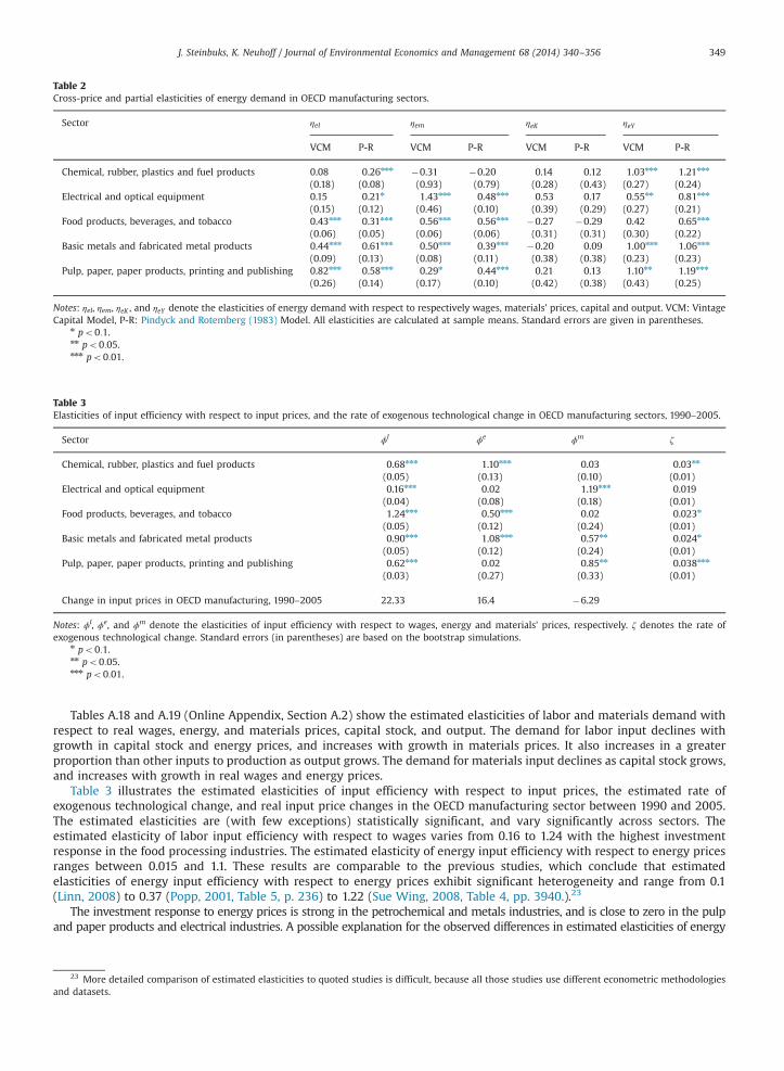
Table 2Cross-price and partial elasticities of energy demand in OECD manufacturing sectors.

Sector ηel ηem ηeK ηeY

VCM P-R VCM P-R VCM P-R VCM P-R

Chemical, rubber, plastics and fuel products 0.08 0.26nnn �0.31 �0.20 0.14 0.12 1.03nnn 1.21nnn

(0.18) (0.08) (0.93) (0.79) (0.28) (0.43) (0.27) (0.24)Electrical and optical equipment 0.15 0.21n 1.43nnn 0.48nnn 0.53 0.17 0.55nn 0.81nnn

(0.15) (0.12) (0.46) (0.10) (0.39) (0.29) (0.27) (0.21)Food products, beverages, and tobacco 0.43nnn 0.31nnn 0.56nnn 0.56nnn �0.27 �0.29 0.42 0.65nnn

(0.06) (0.05) (0.06) (0.06) (0.31) (0.31) (0.30) (0.22)Basic metals and fabricated metal products 0.44nnn 0.61nnn 0.50nnn 0.39nnn �0.20 0.09 1.00nnn 1.06nnn

(0.09) (0.13) (0.08) (0.11) (0.38) (0.38) (0.23) (0.23)Pulp, paper, paper products, printing and publishing 0.82nnn 0.58nnn 0.29n 0.44nnn 0.21 0.13 1.10nn 1.19nnn

(0.26) (0.14) (0.17) (0.10) (0.42) (0.38) (0.43) (0.25)

Notes: ηel, ηem, ηeK , and ηeY denote the elasticities of energy demand with respect to respectively wages, materials' prices, capital and output. VCM: VintageCapital Model, P-R: Pindyck and Rotemberg (1983) Model. All elasticities are calculated at sample means. Standard errors are given in parentheses.


Table 3Elasticities of input efficiency with respect to input prices, and the rate of exogenous technological change in OECD manufacturing sectors, 1990–2005.

Sector ϕl ϕe ϕm ζ

Chemical, rubber, plastics and fuel products 0.68nnn 1.10nnn 0.03 0.03nn

(0.05) (0.13) (0.10) (0.01)Electrical and optical equipment 0.16nnn 0.02 1.19nnn 0.019

(0.04) (0.08) (0.18) (0.01)Food products, beverages, and tobacco 1.24nnn 0.50nnn 0.02 0.023n

(0.05) (0.12) (0.24) (0.01)Basic metals and fabricated metal products 0.90nnn 1.08nnn 0.57nn 0.024n

(0.05) (0.12) (0.24) (0.01)Pulp, paper, paper products, printing and publishing 0.62nnn 0.02 0.85nn 0.038nnn

(0.03) (0.27) (0.33) (0.01)

Change in input prices in OECD manufacturing, 1990–2005 22.33 16.4 �6.29

Notes: ϕl, ϕe, and ϕm denote the elasticities of input efficiency with respect to wages, energy and materials' prices, respectively. ζ denotes the rate ofexogenous technological change. Standard errors (in parentheses) are based on the bootstrap simulations.



Tables A.18 and A.19 (Online Appendix, Section A.2) show the estimated elasticities of labor and materials demand withrespect to real wages, energy, and materials prices, capital stock, and output. The demand for labor input declines withgrowth in capital stock and energy prices, and increases with growth in materials prices. It also increases in a greaterproportion than other inputs to production as output grows. The demand for materials input declines as capital stock grows,and increases with growth in real wages and energy prices.

Table 3 illustrates the estimated elasticities of input efficiency with respect to input prices, the estimated rate ofexogenous technological change, and real input price changes in the OECD manufacturing sector between 1990 and 2005.The estimated elasticities are (with few exceptions) statistically significant, and vary significantly across sectors. Theestimated elasticity of labor input efficiency with respect to wages varies from 0.16 to 1.24 with the highest investmentresponse in the food processing industries. The estimated elasticity of energy input efficiency with respect to energy pricesranges between 0.015 and 1.1. These results are comparable to the previous studies, which conclude that estimatedelasticities of energy input efficiency with respect to energy prices exhibit significant heterogeneity and range from 0.1(Linn, 2008) to 0.37 (Popp, 2001, Table 5, p. 236) to 1.22 (Sue Wing, 2008, Table 4, pp. 3940.).23

The investment response to energy prices is strong in the petrochemical and metals industries, and is close to zero in the pulpand paper products and electrical industries. A possible explanation for the observed differences in estimated elasticities of energy

23 More detailed comparison of estimated elasticities to quoted studies is difficult, because all those studies use different econometric methodologiesand datasets.

Fig. 2. Contribution of energy prices and exogenous technological change to energy input efficiency in the U.S. manufacturing industries, 1990–2005.


input efficiency across sectors is the higher energy intensity of the petrochemical and metals industries. The pulp and paperproducts industry is also energy intensive, but investment volumes have been small (therefore also investment response to energyprices) in the observation period. The pulp and paper products industry also has the highest standard error of estimated elasticities,making further comparisons difficult.

The estimated elasticity of materials efficiency with respect to materials' prices varies from 0.57 to 1.19 in the electrical,pulp and paper products and metals industries, and is close to zero in the petrochemical and food processing industries.Table 3 shows that the real price of materials has fallen in all sectors. Weak investment response to falling materials' pricesin the petrochemical and food processing industries would support the hypothesis of asymmetric investment demandresponse to input prices (see e.g., Borenstein et al., 1997; Peltzman, 2000; Gately and Huntington, 2002). The parameter ζ ispositive in all industries, with further inter-industry comparisons difficult to make due to the high standard error of theestimates. The average growth varies between 0.019 and 0.038 across industries, indicating that autonomous technologicalchange increases the input efficiency of capital stock.24 These results are comparable to Sue Wing's (2008) estimates ofenergy efficiency elasticities with respect to autonomous technology improvements in the range of �0.03 to 0.08.25

Fig. 2 shows the estimated effect of energy prices and the exogenous technological change on the efficiency of energy inputbased on the example of the U.S. manufacturing industries. Between 1990 and 2005 the energy efficiency of capital stockincreased in all sectors, ranging from 17% in the electrical industry to 32% in the pulp and paper industry. In less energy-intensive sectors (see Tables A.3–A.7, Online Appendix, Section A.2.), such as the pulp and paper, and electrical industries, morethan 90 percent of energy efficiency improvements are attributable to exogenous technological change. In more energy-intensive industries the contribution of energy prices is larger. In the petrochemical and metals industries, energy pricesrespectively account for 17 and 26 percent of total improvements in energy efficiency. However, even in these industries therelative effect of exogenous technological change is more significant. These results are consistent with Greenwood et al. (1997),who find that investment-specific technological change accounts for the major part of efficiency growth.

Discussion and limitations

Our analysis is based on a novel econometric framework, which expands the traditional estimation of energy, materials,and labor responses to input price changes by including vintages of the capital stock. As with most new modeldevelopments, introducing capital vintages is costly. To make the model estimable we had to make a number of important,and to some extent, restrictive assumptions. Below we discuss these assumptions in greater detail, focusing specifically ontheir implications for our empirical results.

One of the key assumptions of our study is that firms are forward-looking, and form their expectations based on the input pricesat the time of investment. This assumption requires additional explanation, especially in the context of energy prices, as somescholars noted that energy demand responds asymmetrically to energy prices (Gately and Huntington, 2002; Adeyemi and Hunt,

24 Estimate of annual exogenous technological change in the pulp and paper products industries is higher than estimated rates of autonomous energyefficiency improvements at the economy level (0.5–2.5 percent) found in earlier studies. The determinants of technological change at the industry level canbe inferred from a rigorous econometric analysis using a detailed engineering description of production activities and of the innovations to them (Kopp andSmith, 1985), and are beyond the scope of this paper.

25 The opposite sign is used here as Sue Wing (2008) reports the estimates of energy intensity elasticities with respect to autonomous technologyimprovements.


2007), so time lags could matter. We believe that this assumption is justified for the following reasons. First, input prices, and,especially, energy prices are very difficult to forecast, and likely follow a random walk (Pindyck, 1999; Alquist and Kilian, 2010).26

Second, energy costs are a relatively small share of total expenditures for most manufacturing firms, whereas the costs of obtainingaccurate information on factors affecting future costs are non-trivial (Howarth and Andersson, 1993). Third, recent evidence fromrigorous econometric studies based on micro-level data suggest that average consumer beliefs are indistinguishable from a no-change forecast (Allcott et al., 2011; Anderson et al., 2013), and “researchers are likely to be justified in assuming that averageconsumers employ a no-change forecast in most circumstances” (Anderson et al., 2013, p. 401). Finally, lagged energy prices couldmatter over the very long-term, as new technologies penetrate the market, which is not the focus of this study. If instead themarket participants' expectations of input prices were determined by the long-term equilibrium path, current prices should notaffect their investment choices. Correspondingly, the respective elasticity estimates should be close to zero. However, we do obtainsignificant estimates for the response of investment to energy prices, at least for three industries. Therefore, energy priceexpectations seem to vary with current energy prices. These expectations might only vary over the short term with subsequentreversion to a long term trend. In this case our investment elasticity estimates should be interpreted as the lower bounds to theiractual absolute values.

An important limitation of this study is our assumption that the manufacturing industries in OECD countries operate inperfectly competitive product and factor markets, and take input prices as given. This assumption follows the theoreticalliterature discussed above and is useful for simplifying the derivations. Of course both input and product markets of manyindustries, including those studied in this paper, are characterized by some degree of strategic behavior of their marketparticipants. The strategic behavior will have limited impact on both theoretical predictions and the quality of theeconometric estimates to the extent that such behavior results in constant mark-ups charged by the market participants.More important concern for our econometric estimates is an unobserved change in market structure that results inanticipated changes to mark-ups and thus in investment choices that are not explained by current input prices. On theproduction side, strategic behavior can motivate producers to (i) underinvest in production capacity and (ii) reduce theproduction volume. Neither of these decisions should affect the cost minimizing strategy of the manufacturing firms, at leastin the first order, and will therefore not have a significant impact on the elasticity estimates.

A more serious limitation to this study is our assumption of exogenous and constant capital depreciation rates. Many theoreticaland numerical simulation models allow for endogenous life time of capital vintages, implying an endogenous depreciation rate.Unfortunately, this feature is more difficult to implement in empirical assessments. Manufacturing plants do keep track records ofmaintenance and re-investments pursued since commissioning, however this is very difficult to approximate externally. In practice,new additions to capital stock, its replacement, and scraping depend on a number of factors, such as (i) outside investmentopportunities (e.g., many of the OECD energy-intensive industries invested in growing Asian markets with higher expected returnson capital), (ii) global and country-wide macroeconomic fluctuations, and (iii) regulatory policies (e.g., changes in regulationsaffecting labor markets, environmental compliance costs, or market conduct). Incorporating all those factors would go way beyondthe scope of this paper. These caveats notwithstanding, it is important to understand how the potential endogeneity of capitalreplacement rates affects our elasticity estimates. For energy intensive installations high energy prices can incentivize acceleratedreplacement of energy-inefficient plants. If these incentives have a material impact on replacement rates, then higher depreciationrates will provide a further channel, which results in asymmetric energy demand elasticities (Adeyemi and Hunt, 2007). Conversely,our model based on the exogenous replacement rates might provide upward biased estimates for energy price elasticity oftechnology choice.

To further clarify the implications of this assumption for our empirical results, we have conducted sensitivity analysis, imposing5% and 15% rates of depreciation in addition to the initial value of 10%. The results of the sensitivity analysis are summarized in theOnline Appendix, Tables A.20–A.22. The estimated elasticities are robust to these perturbations. The estimates of own-priceelasticities of input demand and cross-price elasticities of energy demand are insensitive to changes in the assumed rate of assetdepreciation. The estimates of elasticities of input efficiency with respect to input prices, and the estimated rate of exogenoustechnological change are little changed for the electrical and pulp and paper industries. For the other three industries we see thatthe elasticities of input efficiency with respect to input prices increase as the depreciation rate declines. This result is consistent withour theoretical framework – longer life of capital stocks raises their ex post replacement costs and induces stronger ex anteinvestment in more efficient capital. The estimated rate of exogenous technological change also changes, declining for thepetrochemical and metals industries, and increasing for the food processing industry. However, given the large standard errors ofthese estimates, we cannot conclude that these differences are significant in the statistical sense.

Simulated effects of a carbon tax

The results of the vintage capital model indicate that energy-price induced improvements in capital stock can be significant indetermining the future energy efficiency of production. Thus energy and climate policies that provide incentives for earlyinvestment in energy efficient capital stock may reduce future energy (including fossil fuel) input consumption. To illustrate the

26 Some energy price developments can be forecast, e.g., due to pre-announced energy and climate policies. Our study refers to the historic responsesto energy price developments, which were largely driven by resource discoveries, technological innovations, macroeconomic fluctuations, and geopoliticaldevelopments – all these factors are rather difficult to anticipate.

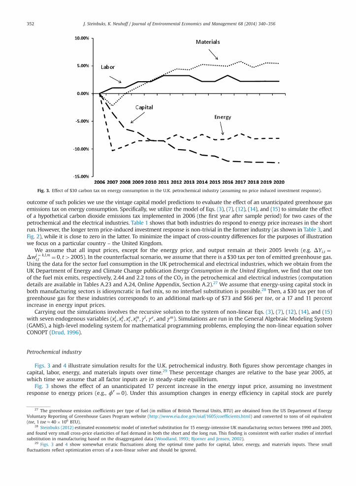
Fig. 3. Effect of $30 carbon tax on energy consumption in the U.K. petrochemical industry (assuming no price induced investment response).


outcome of such policies we use the vintage capital model predictions to evaluate the effect of an unanticipated greenhouse gasemissions tax on energy consumption. Specifically, we utilize the model of Eqs. (3), (7), (12), (14), and (15) to simulate the effectof a hypothetical carbon dioxide emissions tax implemented in 2006 (the first year after sample period) for two cases of thepetrochemical and the electrical industries. Table 1 shows that both industries do respond to energy price increases in the shortrun. However, the longer term price-induced investment response is non-trivial in the former industry (as shown in Table 3, andFig. 2), while it is close to zero in the latter. To minimize the impact of cross-country differences for the purposes of illustrationwe focus on a particular country – the United Kingdom.

We assume that all input prices, except for the energy price, and output remain at their 2005 levels (e.g. ΔYi;t ¼Δwj ¼ k;l;m

i;t ¼ 0; t42005). In the counterfactual scenario, we assume that there is a $30 tax per ton of emitted greenhouse gas.Using the data for the sector fuel consumption in the UK petrochemical and electrical industries, which we obtain from theUK Department of Energy and Climate Change publication Energy Consumption in the United Kingdom, we find that one tonof the fuel mix emits, respectively, 2.44 and 2.2 tons of the CO2 in the petrochemical and electrical industries (computationdetails are available in Tables A.23 and A.24, Online Appendix, Section A.2).27 We assume that energy-using capital stock inboth manufacturing sectors is idiosyncratic in fuel mix, so no interfuel substitution is possible.28 Then, a $30 tax per ton ofgreenhouse gas for these industries corresponds to an additional mark-up of $73 and $66 per toe, or a 17 and 11 percentincrease in energy input prices.

Carrying out the simulations involves the recursive solution to the system of non-linear Eqs. (3), (7), (12), (14), and (15)with seven endogenous variables (xlt ; x

kt ; x

et ; x

mt ; γ

l, γe, and γm). Simulations are run in the General Algebraic Modeling System(GAMS), a high-level modeling system for mathematical programming problems, employing the non-linear equation solverCONOPT (Drud, 1996).

Petrochemical industry

Figs. 3 and 4 illustrate simulation results for the U.K. petrochemical industry. Both figures show percentage changes incapital, labor, energy, and materials inputs over time.29 These percentage changes are relative to the base year 2005, atwhich time we assume that all factor inputs are in steady-state equilibrium.

Fig. 3 shows the effect of an unanticipated 17 percent increase in the energy input price, assuming no investmentresponse to energy prices (e.g., ϕe ¼ 0). Under this assumption changes in energy efficiency in capital stock are purely

27 The greenhouse emission coefficients per type of fuel (in million of British Thermal Units, BTU) are obtained from the US Department of EnergyVoluntary Reporting of Greenhouse Gases Program website (http://www.eia.doe.gov/oiaf/1605/coefficients.html) and converted to tons of oil equivalent(toe, 1 toe� 40� 106 BTU).

28 Steinbuks (2012) estimated econometric model of interfuel substitution for 15 energy-intensive UK manufacturing sectors between 1990 and 2005,and found very small cross-price elasticities of fuel demand in both the short and the long run. This finding is consistent with earlier studies of interfuelsubstitution in manufacturing based on the disaggregated data (Woodland, 1993; Bjorner and Jensen, 2002).

29 Figs. 3 and 4 show somewhat erratic fluctuations along the optimal time paths for capital, labor, energy, and materials inputs. These smallfluctuations reflect optimization errors of a non-linear solver and should be ignored.

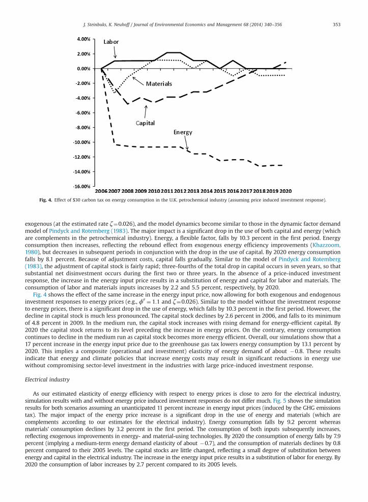
http://www.eia.doe.gov/oiaf/1605/coefficients.html

Fig. 4. Effect of $30 carbon tax on energy consumption in the U.K. petrochemical industry (assuming price induced investment response).


exogenous (at the estimated rate ζ¼0.026), and the model dynamics become similar to those in the dynamic factor demandmodel of Pindyck and Rotemberg (1983). The major impact is a significant drop in the use of both capital and energy (whichare complements in the petrochemical industry). Energy, a flexible factor, falls by 10.3 percent in the first period. Energyconsumption then increases, reflecting the rebound effect from exogenous energy efficiency improvements (Khazzoom,1980), but decreases in subsequent periods in conjunction with the drop in the use of capital. By 2020 energy consumptionfalls by 8.1 percent. Because of adjustment costs, capital falls gradually. Similar to the model of Pindyck and Rotemberg(1983), the adjustment of capital stock is fairly rapid; three-fourths of the total drop in capital occurs in seven years, so thatsubstantial net disinvestment occurs during the first two or three years. In the absence of a price-induced investmentresponse, the increase in the energy input price results in a substitution of energy and capital for labor and materials. Theconsumption of labor and materials inputs increases by 2.2 and 5.5 percent, respectively, by 2020.

Fig. 4 shows the effect of the same increase in the energy input price, now allowing for both exogenous and endogenousinvestment responses to energy prices (e.g., ϕe ¼ 1:1 and ζ¼0.026). Similar to the model without the investment responseto energy prices, there is a significant drop in the use of energy, which falls by 10.3 percent in the first period. However, thedecline in capital stock is much less pronounced. The capital stock declines by 2.6 percent in 2006, and falls to its minimumof 4.8 percent in 2009. In the medium run, the capital stock increases with rising demand for energy-efficient capital. By2020 the capital stock returns to its level preceding the increase in energy prices. On the contrary, energy consumptioncontinues to decline in the medium run as capital stock becomes more energy efficient. Overall, our simulations show that a17 percent increase in the energy input price due to the greenhouse gas tax lowers energy consumption by 13.1 percent by2020. This implies a composite (operational and investment) elasticity of energy demand of about �0.8. These resultsindicate that energy and climate policies that increase energy costs may result in significant reductions in energy usewithout compromising sector-level investment in the industries with large price-induced investment response.

Electrical industry

As our estimated elasticity of energy efficiency with respect to energy prices is close to zero for the electrical industry,simulation results with and without energy price induced investment responses do not differ much. Fig. 5 shows the simulationresults for both scenarios assuming an unanticipated 11 percent increase in energy input prices (induced by the GHG emissionstax). The major impact of the energy price increase is a significant drop in the use of energy and materials (which arecomplements according to our estimates for the electrical industry). Energy consumption falls by 9.2 percent whereasmaterials' consumption declines by 3.2 percent in the first period. The consumption of both inputs subsequently increases,reflecting exogenous improvements in energy- and material-using technologies. By 2020 the consumption of energy falls by 7.9percent (implying a medium-term energy demand elasticity of about �0.7), and the consumption of materials declines by 0.8percent compared to their 2005 levels. The capital stocks are little changed, reflecting a small degree of substitution betweenenergy and capital in the electrical industry. The increase in the energy input price results in a substitution of labor for energy. By2020 the consumption of labor increases by 2.7 percent compared to its 2005 levels.

Fig. 5. Effect of $30 carbon tax on energy consumption in the U.K. electrical industry.


Similar to the petrochemical industry, our results indicate that an increase in energy prices may result in significantreductions in energy use without compromising sector-level investment. In the case of the electrical industry, this finding isdriven by an entirely different channel – weak complementarity between energy and capital.

Concluding remarks

We have expanded the traditional estimation of energy, materials, and labor responses to input price changes byincluding vintages of the capital stock. The model accounts for transitional dynamics of capital in response to energy prices,and allows for more efficient use of inputs to production by choosing more efficient technologies at the time of investment.

In order to test the model, we develop a new dataset for 19 OECD countries and five manufacturing industries over theperiod 1990–2005. At the industry level, the explanatory value of the model with vintage capital stock is significantlyimproved. The conventional dynamic factor demand model of energy demand is rejected for all industries in the sample.The estimated elasticities of energy input efficiency with respect to energy prices vary between 0.015 and 1.1. Theinvestment response to energy prices thus varies significantly across manufacturing industries, being significant in some(typically more energy-intensive) industries and negligible in others. We also find substantial autonomous improvements inthe energy efficiency of capital stock over recent decades, ranging between 2 and 4 percent per annum. This result indicatesthat differences in the estimated investment response to energy prices from previous empirical studies can be, to someextent, attributed to the aggregation problem.

An important finding of this paper is that energy and climate policies aimed at reductions in fossil fuel emissions canresult in substantial reductions in energy use in energy intensive sectors. The results of our counterfactual simulationsindicate that an increase in energy prices results in a considerable decline in energy use. The combined operational andinvestment own-price elasticity of energy demand based on these simulations is between 0.7 and 0.8. At the same time, thereductions in capital stock in the medium run are negligible. In the petrochemical industry, the decline in capital stockresulting from short-run energy-capital complementarity is offset by increasing demand for more energy-efficient capital. Inthe electrical industry, energy-using capital stocks are little changed because of weak complementarity between energy andcapital.

In further work it will be interesting to address the data-driven limitations of this study and explore the robustness ofour results by (1) expanding the observation period beyond 1990–2005; (2) extending the analysis to a larger number ofindustries; and (3) including non-OECD countries in the dataset.

Acknowledgments

The authors are especially grateful to David Newbery for his invaluable contribution to this paper. We also thank TerryBarker, Geoff Bertram, Carol Dahl, Gerald Granderson, Michael Grubb, Richard Horan, Lester Hunt, Fred Joutz, Joshua Linn,Gilbert Metcalf, M. Hashem Pesaran, David Popp (the editor), Paul Preckel, John Reilly, Alan Sanstad, Mike Toman, IanWalker, Ian Sue Wing, ThomasWeber, Anthony Yezer, 3 anonymous reviewers, and seminar participants at Central European


University, Miami University, Purdue University, University of Cambridge, University of Lancaster, University of Surrey, theWorld Bank, the EPRG Winter Research Seminar, American Economic Association Annual Meetings, European EconomicAssociation Annual Symposium, IAEE Annual European Conference, Royal Economic Society Annual Meetings, and SupergenFlexNet General Assembly for helpful comments and suggestions. Special thanks to Sergiy Radyakin for helping us withparallel computing of simulated results and to Andreia Meshreky for outstanding research assistance. Responsibility for thecontent of the paper is the authors' alone and does not necessarily reflect the views of their institutions, or membercountries of the World Bank. Financial support from UK Engineering and Physical Science Research Council, Grant SupergenFlexnet is greatly acknowledged.

Appendix A. Supplementary material

Supplementary data associated with this paper can be found in the online version at http://dx.doi.org/10.1016/j.jeem.2014.07.003.

References

Adeyemi, O., Hunt, L., 2007. Modelling OECD industrial energy demand: asymmetric price responses and energy-saving technical change. Energy Econ.29 (4), 693–709.

Agnolucci, P., 2009. The energy demand in the british and german industrial sectors: heterogeneity and common factors. Energy Econ. 31 (1), 175–187.Allcott, H., Mullainathan, S., Taubinsky, D., 2011. Driving toward paternalism? evaluating behavioral rationales for fuel economy policy. Am. Econ. Rev. 101

(2), 98–104.Alquist, R., Kilian, L., 2010. What do we learn from the price of crude oil futures? J. Appl. Econom. 25 (4), 539–573.Anderson, S., Kellogg, R., Sallee, J., 2013. What do consumers believe about future gasoline prices? J. Environ. Econ. Manag. 66, 383–403.Andrikopoulos, A., Brox, J., Paraskevopoulos, C., 1989. Interfuel and interfactor substitution in ontario manufacturing, 1962–1982. Appl. Econ. 21, 1–15.Arellano, M., Bover, O., 1995. Another look at the instrumental variable estimation of error-components models. J. Econom. 68 (1), 29–51.Atkeson, A., Kehoe, P., 1999. Models of energy use: putty-putty versus putty-clay. Am. Econ. Rev. 89 (4), 1028–1043.Azomahou, T.T., Boucekkine, R., Nguyen-Van, P., 2012. Vintage capital and the diffusion of clean technologies. Int. J. Econ. Theory 8 (3), 277–300.Baltagi, B., Griffin, J., 1988. A general index of technical change. J. Polit. Econ. 96 (1), 20–41.Barker, T., Ekins, P., Johnstone, N., 1995. Global Warming and Energy Demand. Routledge, London and New York.Barnett, W., Geweke, J., Wolfe, M., 1991. Seminonparametric Bayesian estimation of the asymptotically ideal production model. J. Econom. 49 (1–2), 5–50.Benhabib, J., Rusticini, A., 1991. Vintage capital, investment, and growth. J. Econ. Theory 55, 323–339.Berndt, E., Wood, D., 1975. Technology, prices, and the derived demand for energy. Rev. Econ. Stat. 57 (3), 259–268.Berndt, E., Morrison, C., Watkins, G., 1981. Dynamic models of energy demand: an assessment and comparison. In: Berndt, E., Field, B. (Eds.), Measuring and

Modeling Natural Resource Substitution, MIT Press, Cambridge, MA.Bjorner, T., Jensen, H., 2002. Interfuel substitution within industrial companies: an analysis based on panel data at company level. Energy J. 23 (2), 27–50.Blundell, R., Bond, S., 1998. Initial conditions and moment restrictions in dynamic panel data models. J. Econom. 87 (1), 115–143.Borenstein, S., Cameron, A., Gilbert, R., 1997. Do gasoline prices respond asymmetrically to crude oil price changes? Q. J. Econ. 112 (1), 305–339.Boucekkine, R., Germain, M., Licandro, O., 1997. Replacement echoes in the vintage capital growth model. J. Econ. Theory 74 (2), 333–348.Brack, D., Grubb, M., Windram, C., 2000. International Trade and Climate Change Policies. Earthscan, London, UK.Burnside, C., 1996. Production function regressions, returns to scale, and externalities. J. Monet. Econ. 37 (2), 177–201.Chari, V.V., Hopenhayn, H., 1991. Vintage human capital, growth, and the diffusion of new technology. J. Polit. Econ. 99 (6), 1142–1165.Cho, W., Nam, K., Pagán, J., 2004. Economic growth and interfactor/interfuel substitution in Korea. Energy Econ. 26 (1), 31–50.Diewert, W.E., 1980. Aggregation problems in the measurement of capital. In: Usher, D. (Ed.), The Measurement of Capital, University of Chicago Press,

Chicago, IL, pp. 433–538.Diewert, W., Fox, K., 2008. On the estimation of returns to scale, technical progress and monopolistic markups. J. Econom. 145 (1–2), 174–193.Drud, A., 1996. CONOPT: A System for Large Scale Nonlinear Optimization. ARKI Consulting and Development, Bagsvaerd, Denmark.Enevoldsen, M.K., Ryelund, A.V., Andersen, M.S., 2007. Decoupling of industrial energy consumption and CO2-emissions in energy-intensive industries in

Scandinavia. Energy Econ. 29 (4), 665–692.Frondel, M., 2004. Empirical assessment of energy-price policies: the case for cross-price elasticities. Energy Policy 32 (8), 989–1000.Fuss, M., 1977. The structure of technology over time: a model for testing the ‘putty-clay’ hypothesis. Econometrica 45 (8), 1797–1821.Gately, D., Huntington, H., 2002. The asymmetric effects of changes in price and income on energy and oil demand. Energy J. 23 (1), 19–56.Greenwood, J., Hercowitz, Z., Krusell, P., 1997. Long-run implications of investment-specific technological change. Am. Econ. Rev. 87 (3), 342–362.Griffin, J., Gregory, P., 1976. An intercountry translog model of energy substitution responses. Am. Econ. Rev. 66 (5), 845–857.Griffin, J., Schulman, C., 2005. Price asymmetry: a proxy for energy saving technical change?. Energy J. 26 (2), 1–21.Haas, R., Schipper, L., 1998. Residential energy demand in OECD-countries and the role of irreversible efficiency improvements. Energy Econo. 20 (4),

421–442.Hart, R., 2004. Growth, environment and innovation—a model with production vintages and environmentally oriented research. J. Environ. Econ. Manag.

48 (3), 1078–1098.Howarth, R., Andersson, B., 1993. Market barriers to energy efficiency. Energy Econ. 15 (4), 262–272.International Energy Agency, 2008. Energy Prices and Taxes, 4th Quarter 2008. OECD/IEA, Paris, France.Jacoby, H.D., SueWing, I., 1999. Adjustment time, capital malleability and policy cost. Energy J. 20 (S), 73–92.Johansen, L., 1959. Substitution versus fixed production coefficients in the theory of economic growth: a synthesis. Econometrica 27 (2), 157–176.Jorgenson, D., 1980. Accounting for capital. In: vonFurstenberg, G. (Ed.), Capital Efficiency and Growth, Ballinger, Cambridge, MA, pp. 251–319.Jorgenson, D., Fraumeni, B., 1981. Relative prices and technical change. in: Berndt, E.R. (Ed.), Modeling and Measuring Natural Resource Substitution.Jorgenson, D., Gollop, F., Fraumeni, B., 1987. Productivity and US Economic Growth. Harvard University Press, Cambridge, MA.Jorgenson, D., Ho, M., Stiroh, K., 2005. Information Technology and the American Growth Resurgence. MIT Press, Cambridge, MA.Judd, K.L., 1998. Numerical Methods in Economics. The MIT press.Khazzoom, J., 1980. Economic implications of mandated efficiency in standards for household appliances. Energy J. 1 (4), 21–40.Koetse, M.J., De Groot, H.L.F., Florax, R.J.G.M., 2008. Capital-energy substitution and shifts in factor demand: a meta-analysis. Energy Econ. 30 (5),

2236–2251.Koopmans, C.C., te Velde, D.W., 2001. Bridging the energy efficiency gap: using bottom-up information in a top-down energy demand model. Energy Econ.

23 (1), 57–75.Kopp, R., Smith, V., 1985. The measurement of non-neutral technological change. Int. Econ. Rev. 26 (1), 135–159.



http://refhub.elsevier.com/S0095-0696(14)00068-0/sbref1
























































Linn, J., 2008. Energy prices and the adoption of energy-saving technology. Econ. J. 118, 1986–2012.Malcomson, J.M., 1975. Replacement and the rental value of capital equipment subject to obsolescence. J. Econ. Theory 10 (1), 24–41.Meijers, H.H. M., 1994. On the Diffusion of Technologies in a Vintage Framework: Theoretical Considerations and Empirical Results (Ph.D. thesis).Metcalf, G., 2008. An empirical analysis of energy intensity and its determinants at the state level. Energy J. 29 (3), 1–26.Mulder, P., de Groot, H.L., Hofkes, M.W., 2003. Explaining slow diffusion of energy-saving technologies; a vintage model with returns to diversity and

learning-by-using. Resour. Energy Econ. 25 (1), 105–126.Newell, R., Jaffe, A., Stavins, R., 1999. The induced innovation hypothesis and energy-saving technological change. Q. J. Econ. 114 (3), 941–975.O'Mahony, M., Timmer, M.P., 2009. Output, input and productivity measures at the industry level: the EU KLEMS database. Econ. J. 119 (538), F374–F403.Peltzman, S., 2000. Prices rise faster than they fall. J. Polit. Econ. 108 (3), 466–502.Pérez-Barahona, A., Zou, B., 2006. A comparative study of energy saving technical progress in a vintage capital model. Resour. Energy Econ. 28, 181–191.Pindyck, R., 1999. The long-run evolution of energy prices. Energy J. 20 (2), 1–27.Pindyck, R., Rotemberg, J., 1983. Dynamic factor demands and the effects of energy price shocks. Am. Econ. Rev. 73, 1066–1079.Popp, D., 2001. The effect of new technology on energy consumption. Resour. Energy Econ. 23 (3), 215–240.Popp, D., 2002. Induced innovation and energy prices. Am. Econ. Rev. 92 (1), 160–180.Sheshinski, E., 1967. Balanced growth and stability in the Johansen vintage model. Rev. Econ. Stud. 34 (2), 239–248.Solow, R.M., Tobin, J., von Weizsäcker, C.C., Yaari, M., 1966. Neoclassical growth with fixed factor proportions. Rev. Econ. Stud. 33 (2), 79–115.Steinbuks, J., 2012. Interfuel substitution and energy use in the UK manufacturing sector. Energy J. 33 (1), 1–30.Sue Wing, I., 2008. Explaining the declining energy intensity of the US economy. Resour. Energy Econ. 30 (1), 21–49.Timmer, M., O Mahony, M., van Ark, B., 2007. EU KLEMS Growth and Productivity Accounts: An Overview. Working Paper, University of Groningen,

University of Birmingham.Urga, G., Walters, C., 2003. Dynamic translog and linear logit models: a factor demand analysis of interfuel substitution in US industrial energy demand.

Energy Econ. 25 (1), 1–21.Webster, M., Paltsev, S., Reilly, J., 2008. Autonomous efficiency improvement or income elasticity of energy demand: does it matter?. Energy Econ. 30 (6),

2785–2798.Woodland, A., 1993. A micro-econometric analysis of the industrial demand for energy in NSW. Energy J. 14 (2), 57–89.























assessing energy price induced improvements in efficiency of capital in oecd manufacturing...

Documents