Earth Syst. Dynam., 9, 339–357, 2018https://doi.org/10.5194/esd-9-339-2018© Author(s) 2018. This work is distributed underthe Creative Commons Attribution 4.0 License.

Assessing carbon dioxide removal through global andregional ocean alkalinization under high

and low emission pathways

Andrew Lenton1,2, Richard J. Matear1, David P. Keller3, Vivian Scott4, and Naomi E. Vaughan5

1CSIRO Oceans and Atmosphere, Hobart, Australia2Antarctic Climate and Ecosystems Co-operative Research Centre, Hobart, Australia

3GEOMAR Helmholtz Centre for Ocean Research, Kiel, Germany4School of Geosciences, University of Edinburgh, Edinburgh, UK

5Tyndall Centre for Climate Change Research, School of Environmental Sciences,University of East Anglia, Norwich, UK

Correspondence: Andrew Lenton (andrew.lenton@csiro.au)

Received: 23 October 2017 – Discussion started: 1 November 2017Revised: 26 January 2018 – Accepted: 9 March 2018 – Published: 6 April 2018

Abstract. Atmospheric carbon dioxide (CO2) levels continue to rise, increasing the risk of severe impacts onthe Earth system, and on the ecosystem services that it provides. Artificial ocean alkalinization (AOA) is capableof reducing atmospheric CO2 concentrations and surface warming and addressing ocean acidification. Here, wesimulate global and regional responses to alkalinity (ALK) addition (0.25 PmolALK yr−1) over the period 2020–2100 using the CSIRO-Mk3L-COAL Earth System Model, under high (Representative Concentration Pathway8.5; RCP8.5) and low (RCP2.6) emissions. While regionally there are large changes in alkalinity associated withlocations of AOA, globally we see only a very weak dependence on where and when AOA is applied. On aglobal scale, while we see that under RCP2.6 the carbon uptake associated with AOA is only∼ 60 % of the total,under RCP8.5 the relative changes in temperature are larger, as are the changes in pH (140 %) and aragonitesaturation state (170 %). The simulations reveal AOA is more effective under lower emissions, therefore thehigher the emissions the more AOA is required to achieve the same reduction in global warming and oceanacidification. Finally, our simulated AOA for 2020–2100 in the RCP2.6 scenario is capable of offsetting warmingand ameliorating ocean acidification increases at the global scale, but with highly variable regional responses.

1 Introduction

Atmospheric carbon dioxide (CO2) levels continue to rise asa result of human activities. Recent studies have suggestedthat even deep cuts in emissions may not be sufficient toavoid severe impacts on the Earth system, and the ecosystemservices that it provides (Gasser et al., 2015). Recent inter-national negotiations (UNFCCC, 2015) have agreed to limitglobal warming to well below 2 ◦C. The application of car-bon dioxide removal (CDR), sometimes referred to as “neg-ative emissions”, appears to be required to achieve this goal,as emission reductions alone are likely to be insufficient (Ro-gelj et al., 2016). In this context, there is an urgent need to

assess how CDR could help either mitigate climate changeor even reverse it, and to understand the potential risks andbenefits of different options.

While warming represents an imminent global threatwhich is already significantly impacting the natural environ-ment (Hughes et al., 2017), ocean acidification poses an ad-ditional and equally significant threat to the marine environ-ment. At present the oceans take up about 28 % of anthro-pogenic CO2 emitted annually (Le Quéré et al., 2015). AsCO2 is taken up by the ocean it changes its chemical equilib-rium, reducing the carbonate ion concentration and decreas-ing pH, collectively known as ocean acidification. Further-more, as the ocean continues to take up carbon the buffer-

Published by Copernicus Publications on behalf of the European Geosciences Union.

340 A. Lenton et al.: Ocean alkalinization under high and low emissions

ing capacity or Revelle factor (Revelle and Suess, 1957) ofthe seawater decreases, thereby accelerating the rate of oceanacidification.

Ocean acidification is the unavoidable consequence of ris-ing atmospheric CO2 levels and will impact the entire marineecosystem – from plankton at the base through to higher-trophic species at the top. Potential impacts include changesin calcification, fecundity, organism growth and physiology,species composition and distributions, food web structure,and nutrient availability (Doney et al., 2012; Fabry et al.,2008; Iglesias-Rodriguez et al., 2008; Munday et al., 2009,2010). Within this century, the impacts of ocean acidifica-tion will increase in proportion to emissions (Gattuso et al.,2015). Furthermore, these changes will be long-lasting, per-sisting for centuries or longer even if emissions are halted(Frolicher and Joos, 2010).

To date, many different CDR techniques have been pro-posed (Shepherd et al., 2009; National Research Council,2015). Their primary purpose is to reduce atmospheric CO2levels, and thus most CDR methods will also reduce the im-pacts of ocean acidification, although some proposed tech-niques such as ocean pipes (Lovelock and Rapley, 2007)and micro-nutrient addition (Keller et al., 2014) may actu-ally lead to a regional acceleration of ocean acidification insurface waters.

Artificial ocean alkalinization (AOA), through altering thechemistry of seawater, both enhances ocean carbon uptake(thereby reducing atmospheric CO2), and simultaneously re-verses ocean acidification and increases the ocean’s bufferingcapacity. AOA can be thought of as a massive acceleration ofthe natural processes of chemical weathering of minerals thathave played a role in modulating the climate on geologicaltimescales (Zeebe, 2012; Colbourn et al., 2015; Sigman andBoyle, 2000).

Specifically, as alkalinity enters the ocean, the pH in-creases leading to an elevated carbonate ion concentration, areduction in the hydrogen ion concentration, and a decreasein the concentration of aqueous CO2 (or pCO2). This in turnenhances the disequilibrium of CO2 between the ocean andatmosphere (or 1pCO2 =pCOocean

2 −pCOatmosphere2 ) lead-

ing to increased ocean carbon uptake, and a reduction in theatmospheric CO2 concentration. These increases in pH andcarbonate ion concentration thus reverse the ocean acidifica-tion due to uptake of anthropogenic CO2.

Kheshgi (1995) first proposed AOA as a method of CDR.Renforth and Henderson (2017) review the early experimen-tal, engineering, and modelling work undertaken to inves-tigate AOA. From the observational perspective, we drawparticular attention to the experimental work of Albright etal. (2016) which provided an in situ demonstration of local-ized AOA to offset the observed changes in ocean acidifica-tion on the Great Barrier Reef which have occurred since thepre-industrial period.

Several modelling studies have explored the impacts ofAOA both on carbon sequestration and ocean acidifica-tion. Using ocean-only biogeochemical models, Kohler etal. (2013) explored AOA via olivine addition. Olivine, in ad-dition to increasing alkalinity also adds iron and silicic acid,both of which can enhance ocean productivity (Jickells etal., 2005; Ragueneau et al., 2000). Kohler et al. (2013) esti-mated the response of atmospheric CO2 levels and pH to dif-ferent levels of olivine addition over the period 2000–2010,and this was later extended to 2100 by Hauck et al. (2016).These studies demonstrate a global impact that appears toscale with the amount of olivine added. Importantly, Kohleret al. (2013) showed that the global effect of alkalinity addedalong shipping routes (as an analogue for practical imple-mentation) was not significantly different from that of alka-linity added in a highly idealized uniform manner.

Ilyina et al. (2013) explored the potential of AOA to mit-igate rising atmospheric CO2 levels and ocean acidificationin ocean-only biogeochemical simulations, and they showedthat AOA has the potential to ameliorate future changes dueto high CO2 emissions. They did not limit the amount ofAOA, as their goal was to offset the projected future changes,and showed that the amount of AOA required to do thiswould drive the carbonate system to levels well above pre-industrial levels. Ilyina et al. (2013) also conclude that localAOA could potentially be used to offset the impacts of oceanacidification, with enhanced CO2 uptake being only a sidebenefit. This regional approach was explored further by Fenget al. (2016) who suggested that local AOA in the tropicalocean, in areas of high coral calcification, has the potentialto offset the impacts of future rising atmospheric CO2 levelsunder a high emissions scenario (RCP8.5). This study alsorevealed strong regional sensitivities in the response of oceanacidification related to the locations in which it was applied.

Several other studies have estimated the response of theEarth system to AOA. Gonzalez and Ilyina (2016) usedan Earth system model (ESM) to estimate the AOA re-quired to reduce atmospheric concentrations from a highemissions scenario (RCP8.5) to the medium emissions sce-nario (RCP4.5). They estimated that to mitigate the asso-ciated 1.5 K warming difference, via reducing atmosphericCO2 concentrations by ∼ 400 ppm, an addition of 114 Pmolof alkalinity (between 2018 and 2100) would be required,and it would come at the cost of very large (unprecedented)changes in ocean chemistry.

Keller et al. (2014) used an Earth system model of interme-diate complexity (EMIC) to explore the impacts of AOA overthe period 2020–2100 arising from a globally uniform addi-tion of alkalinity (0.25 PmolALK yr−1), an amount based onthe estimated carrying capacity of global shipping followingKohler et al. (2013). Keller et al. (2014) showed that AOA ledto a reduction in atmospheric CO2 of 166 PgC (or∼ 78 ppm),a net surface air temperature cooling of 0.26 K and a globalincrease in ocean pH of 0.06 in the period 2020–2100.

Earth Syst. Dynam., 9, 339–357, 2018 www.earth-syst-dynam.net/9/339/2018/

A. Lenton et al.: Ocean alkalinization under high and low emissions 341

To date, not all modelling studies have been emissionsdriven, and this is important as potential climate and carboncycle feedbacks may not have been accounted for. Capturingthese feedbacks is critical as they have the potential to signifi-cantly increase atmospheric CO2 concentrations (Jones et al.,2016). Further, no studies have explored the impact of AOAunder low emissions scenarios such as RCP2.6. This is im-portant because scenarios that limit warming to 2 ◦C or less,currently assume considerable land-based CDR via afforesta-tion and/or Biomass energy with carbon capture and storage(BECCS). Furthermore, the feasibility of these approaches isincreasingly questioned due in part to limited land (Smith etal., 2016), whereas the potential CDR capacity of the oceansis orders of magnitude greater (Scott et al., 2015).

In this work, we use a fully coupled ESM (CSIRO-Mk3L-COAL), which includes climate and carbon feedbacks, to in-vestigate the impact of AOA on the carbon cycle, global sur-face warming (2 m surface air temperature), and the oceanacidification response to the global and regional AOA exper-iments under the high (RCP8.5) and low (RCP2.6) emissionsscenarios.

2 Methods

2.1 Model description

The model simulations were performed using the CSIRO-Mk3L-COAL (Carbon, Ocean, Atmosphere, Land) ESMwhich includes climate–carbon interactions and feedbacks(Matear and Lenton, 2014; Q. Zhang et al., 2014). The oceancomponent of the ESM has a resolution of 2.8◦ by 1.6◦ with21 vertical levels. The ocean biogeochemistry is based onLenton and Matear (2007) and Matear and Hirst (2003) sim-ulating the distributions of phosphate, oxygen, dissolved in-organic carbon, and alkalinity in the ocean. The model sim-ulates particulate inorganic carbon (PIC) production as afunction of particulate organic carbon (POC) production viathe rain ratio (9 %) following Yamanaka and Tajika (1996).This ocean biogeochemical model was shown to simulate theobserved distributions of total carbon and alkalinity in theocean (Matear and Lenton, 2014) and phosphate (Duteil etal., 2012).

The atmosphere resolution is 5.6◦× 3.2◦ with 18 verticallayers. The land surface scheme uses CABLE (Best et al.,2015) coupled to CASA-CNP (Wang et al., 2010; Mao etal., 2011) which simulates biogeochemical cycles of carbon,nitrogen, and phosphorus in plants and soils. The responseof the land carbon cycle was shown to simulate the observedbiogeochemical fluxes and pools on the land surface (Wanget al., 2010).

To quantify the changes in ocean acidification, we cal-culate pH changes on the total scale following the rec-ommendation of Riebesell et al. (2010). To calculate thechanges of carbonate saturation state, we use the equationof Mucci (1983).

2.2 Model experimental design

Our ESM was spun up under a pre-industrial atmosphericCO2 concentration of 284.7 ppm, until the simulated climatewas stable (> 2000 years) (Phipps et al., 2012). From thespun-up initial climate state, the historical simulation (1850–2005) was performed using the historical atmospheric CO2concentrations as prescribed by the CMIP5 simulation pro-tocol (Taylor et al., 2012).

Following the historical concentration pathway from 2006onward, two different future projections to 2100 were madeusing the atmospheric CO2 emissions corresponding tothe Representative Concentration Pathways of low emis-sions (RCP2.6) and high emissions (RCP8.5 or “business asusual”) (Taylor et al., 2012). All simulations include the forc-ing due to non-CO2 greenhouse gas concentrations (Tayloret al., 2012). We define RCP8.5 and RCP2.6 as our controlcases for the corresponding experiments below.

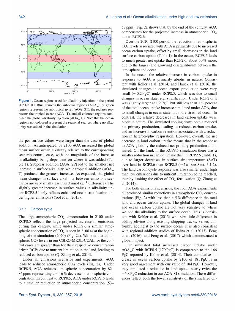
In the period 2020–2100, we undertook a number of AOAexperiments using a fixed quantity of 0.25 Pmol yr−1 of al-kalinity, a similar amount to that used by Keller et al. (2014).Consistent with this study, we applied AOA in the sur-face ocean all year round in ice-free regions, set to be be-tween 60◦ S and 70◦ N (note that this ignores the presenceof seasonal sea ice in some small regions). For each of thetwo emissions scenarios, we considered four different re-gional applications of AOA, shown in Fig. 1. These are:(i) AOA globally (AOA_G) between 60◦ S and 70◦ N; (ii) thehigher latitudes comprising the subpolar Northern Hemi-sphere oceans (40–70◦ N) and the (ice-free) Southern Ocean(40–60◦ S) (AOA_SP); (iii) the subtropical oceans (15–40◦ Nand 15–40◦ S) (AOA_ST); and (iv) in the equatorial regions(15◦ N–15◦ S) (AOA_T). In this study, we only look at theresponse of the Earth system to alkalinity injection. We donot consider the biogeochemical response to other mineralsand elements that can be associated with the sourcing of alka-linity from the application of finely ground ultra-mafic rockssuch as olivine and forsterite, nor dissolution processes re-quired to increase alkalinity (e.g. Montserrat et al., 2017).

3 Results and discussion

To aid in presenting our results and to compare these withprevious studies, we first discuss the carbon cycle, global sur-face warming (2m surface air temperature), and ocean acidi-fication response to the four different AOA experiments un-der the high (RCP8.5) and low (RCP2.6) emissions scenar-ios. We then look at the regional behaviour of the simulationsin the different AOA experiments.

3.1 Global response

For each emissions scenario, we simulated four differentAOA experiments, which all had the same 0.25 Pmol yr−1

of alkalinity added. In the case of the regional experiments

www.earth-syst-dynam.net/9/339/2018/ Earth Syst. Dynam., 9, 339–357, 2018

342 A. Lenton et al.: Ocean alkalinization under high and low emissions

Figure 1. Ocean regions used for alkalinity injection in the period2020–2100. Blue denotes the subpolar regions (AOA_SP), greenregions represent the subtropical gyres (AOA_ST), the red area rep-resents the tropical ocean (AOA_ T), and all coloured regions com-bined the global alkalinity injection (AOA_ G). Note that the oceanregions not coloured represent the seasonal sea ice, where no alka-linity was added in the simulation.

the per surface values were larger than the case of globaladdition. As anticipated, by 2100 AOA increased the globalmean surface ocean alkalinity relative to the correspondingscenario control case, with the magnitude of the increasein alkalinity being dependent on where it was added (Ta-ble 1). Subpolar addition (AOA_SP) led to the smallest netincrease in surface alkalinity, while tropical addition (AOA_T) produced the greatest increase. As expected, the globalmean changes in surface alkalinity between emissions sce-narios are very small (less than 3 µmol kg−1 difference). Theslightly greater increase in surface values in alkalinity un-der RCP8.5 likely reflects enhanced ocean stratification un-der higher emissions (Yool et al., 2015).

3.1.1 Carbon cycle

The large atmospheric CO2 concentration in 2100 underRCP8.5 reflects the large projected increase in emissionsduring this century, while under RCP2.6 a similar atmo-spheric concentration of CO2 is seen in 2100 as at the begin-ning of the simulation (2020) (Fig. 2a). We note that atmo-spheric CO2 levels in our CSIRO-MK3L-COAL for the con-trol cases are greater than for their respective concentrationdriven RCPs due to nutrient limitation in the land, leading toreduced carbon uptake (Q. Zhang et al., 2014).

Under all emissions scenarios and experiments, AOAleads to reduced atmospheric CO2 levels (Fig. 2a). UnderRCP8.5, AOA reduces atmospheric concentration by 82–86 ppm; representing a ∼ 16 % decrease in atmospheric con-centration. In contrast to RCP8.5, AOA under RCP2.6 leadsto a smaller reduction in atmospheric concentration (53–

58 ppm). Fig. 2a shows that, by the end of the century, AOAcompensates for the projected increase in atmospheric CO2due to RCP2.6.

Over the 2020–2100 period, the reduction in atmosphericCO2 levels associated with AOA is primarily due to increasedocean carbon uptake, offset by small decreases in the landsurface carbon uptake (Table 1). In the ocean, RCP8.5 leadsto much greater net uptake than RCP2.6, about 50 % more,due to the larger (and growing) disequilibrium between theatmosphere and ocean.

In the ocean, the relative increase in carbon uptake inresponse to AOA is primarily abiotic in nature. Consis-tent with Keller et al. (2014) and Hauck et al. (2016) thesimulated changes in ocean export production were verysmall (∼ 0.2 PgC) under RCP8.5, which was due to smallchanges in ocean state, e.g. stratification. Under RCP2.6, itwas slightly larger at 1.2 PgC, but still less than 1 % percentof the total ocean uptake increase simulated under AOA, dueto small changes in ocean state in a more stratified ocean. Incontrast, the relative decreases in land carbon uptake werebiotic in nature. The simulated cooling drove both a reducednet primary production, leading to reduced carbon uptake,and an increase in carbon retention associated with a reduc-tion in heterotrophic respiration. However, overall, the netdecrease in land carbon uptake means that in the responseto AOA globally the reduced net primary production dom-inated. On the land, in the RCP8.5 simulation there was asmaller reduction in carbon uptake than in RCP2.6 (Table 1),due to larger decreases in surface air temperature (SAT)over land in RCP2.6 than RCP8.5 (∼ 2×; see Sect. 3.1.2).The land carbon cycle response was also smaller under highthan low emissions due to nutrient limitation being reached,thereby limiting the effect of CO2 fertilization (Q. Zhang etal, 2014).

For both emissions scenarios, the four AOA experimentsall produced similar reductions in atmospheric CO2 concen-trations (Fig. 2) with less than a 5 % difference in the totalland and ocean carbon uptake. The global changes in landand ocean carbon uptake are not very sensitive to wherewe add the alkalinity to the surface ocean. This is consis-tent with Kohler et al. (2013) who saw little difference inadding olivine along existing shipping tracks, versus uni-formly adding it to the surface ocean. It is also consistentwith regional addition studies of Ilyina et al. (2013), Fenget al. (2016), and Feng et al. (2017) which demonstrated aglobal impact.

Our simulated total increased carbon uptake underAOA_G with RCP8.5 (179 PgC) is comparable to the 166PgC reported by Keller et al. (2014). Their cumulative in-crease in ocean carbon uptake by 2100 of 181 PgC is invery good agreement with our value of 184 PgC. However,they simulated a reduction in land uptake nearly twice the−5.8 PgC reduction in our AOA_G simulation. These differ-ences reflect both the lower sensitivity of the simulated cli-

Earth Syst. Dynam., 9, 339–357, 2018 www.earth-syst-dynam.net/9/339/2018/

A. Lenton et al.: Ocean alkalinization under high and low emissions 343

RCP8.5 RCP2.6

RCP8.5_AOA_SP RCP2.6_AOA_SP

RCP8.5_AOA_G

RCP8.5_AOA_T

RCP8.5_AOA_ST

RCP2.6_AOA_G

RCP2.6_AOA_T

RCP2.6_AOA_ST

RCP8.5 RCP2.6

RCP8.5_AOA_SP RCP2.6_AOA_SP

RCP8.5_AOA_G

RCP8.5_AOA_T

RCP8.5_AOA_ST

RCP2.6_AOA_G

RCP2.6_AOA_T

RCP2.6_AOA_ST

Time (years)

Surf

ace

air t

empe

ratu

re (K

)

pH

Arag

onite

sat

urat

ion

stat

e

Atm

soph

eric

CO

2 con

c. (p

pm)

(a)

(b)

(c)

(d)

Time (years)Time (years)

RCP8.5 RCP2.6

RCP8.5_AOA_SP RCP2.6_AOA_SP

RCP8.5_AOA_G

RCP8.5_AOA_T

RCP8.5_AOA_ST

RCP2.6_AOA_G

RCP2.6_AOA_T

RCP2.6_AOA_ST

RCP8.5 RCP2.6

RCP8.5_AOA_SP RCP2.6_AOA_SP

RCP8.5_AOA_G

RCP8.5_AOA_T

RCP8.5_AOA_ST

RCP2.6_AOA_G

RCP2.6_AOA_T

RCP2.6_AOA_ST

Time (years)

Figure 2. The global mean changes in: atmospheric CO2 concentration (a), surface air temperature (SAT; b), surface ocean pH (c), andaragonite saturation state (d), for high (RCP8.5) and low emissions (RCP2.6) with global and regional AOA in the period 2020–2100.

mate feedbacks in our ESM, and differences in land surfacemodels.

3.1.2 Surface air temperature

In the control simulations, the global mean surface air tem-perature (SAT; 2 m) increased in the period 2020–2100with RCP2.6 simulating a net warming of 0.4± 0.1 K whileRCP8.5 warmed by 2.7± 0.1 K (2081–2100). AOA experi-ments simulated a reduction in global mean SAT relative totheir corresponding control simulation (Fig. 2b). Within eachemissions scenario the global mean SAT decline associatedwith AOA is always greater and more variable over the landthan ocean (Table 1). In the period 2081–2100 we see largermean changes in SAT under RCP2.6 than RCP8.5 primarilydue to differences in atmospheric CO2 growth rate. Krast-ing et al. (2014) showed that the slower rate of emissions,the lower the radiative forcing response. This occurs in re-sponse to the timescales associated with the uptake of heatand carbon. Consequently, under RCP8.5 the atmosphericCO2 growth rate is much faster than RCP2.6, leading to astrong radiative forcing response. This explains why, despitea larger reduction in atmospheric CO2 concentration underRCP8.5, the biggest reduction in global mean SAT occur un-der RCP2.6. These mean changes are also associated withlarge inter-annual variability.

Under RCP2.6, all the AOA experiments keep globalwarming levels much closer to values in 2020 than RCP2.6by the end of this century (2100; Fig. 2b). In contrast, underthe RCP8.5 scenario, none of the AOA experiments have asignificant impact on the projected warming by the end ofthis century (less than 10 %) reflecting the large warmingprojected under high emissions.

Within each of the scenarios, there are some differencesin the magnitude of the cooling within the four differentAOA experiments; however, these are smaller than the inter-annual variability over the last two decades of the simula-tions. Therefore, it appears that the global mean SAT de-cline with AOA is not very sensitive to where the alkalinityis added under either emission scenario.

The global mean cooling associated with AOA_G un-der RCP8.5 (−0.16± 0.08 K; 2081–2100) is close to themean surface air temperature cooling of−0.26 K reported byKeller et al. (2014) for similar levels of AOA. These differ-ences may reflect the simplified atmospheric representationof the University of Victoria (UVic) Earth system model ofintermediate complexity and different climate sensitivities.

3.1.3 Ocean acidification

Here, we quantify changes in ocean acidification in termsof pH and aragonite saturation state changes. We consider

www.earth-syst-dynam.net/9/339/2018/ Earth Syst. Dynam., 9, 339–357, 2018

344 A. Lenton et al.: Ocean alkalinization under high and low emissions

Table 1. For the two RCP scenarios: (a) the relative increase in global mean ocean surface alkalinity (µmol kg−1) between each AOAexperiment and control experiment in 2100; (b) the total integrated additional carbon uptake (in PgC) in the period 2020–2100 in differentexperiment and emissions scenarios, positive denotes enhanced uptake; (c) the differences in global mean surface air temperature in theperiod 2081–2100 (2090) and associated standard deviation (1σ ) (K; SAT; 2 m) for the four different AOA experiments for each emissionscenario, relative to the same emission scenario with no AOA.

AOA_G AOA_SP AOA_ ST AOA_T

(a) Relative increase in global mean ocean surface alkalinity (µmol kg−1) in 2100

RCP8.5 108.3 79.7 115.1 129.8RCP2.6 105.1 74.4 112.9 127.1

(b) Total integrated additional carbon uptake (in PgC) in the period 2020–2100

RCP8.5 Total 178.6 183.3 180.7 174.5Ocean 184.4 188.1 185.1 177.2Land −5.8 −4.8 −4.4 −2.7

RCP2.6 Total 121.1 122.1 122.0 116.0Ocean 143.1 145.2 143.1 139.2Land −22.1 −24.1 −21.2 −23.1

(c) Differences in global mean surface air temperature in the period 2081–2100 (2090)and associated standard deviation (1σ ) (K; SAT; 2 m)

RCP8.5 Total −0.16± 0.08 −0.13± 0.10 −0.08± 0.05 −0.14± 0.06Ocean −0.14± 0.07 −0.11± 0.07 −0.06+0.03 −0.12± 0.05Land −0.22± 0.15 −0.18± 0.20 −0.13± 0.14 −0.19± 0.11

RCP2.6 Total −0.25± 0.08 −0.23± 0.08 −0.20± 0.09 −0.16± 0.06Ocean −0.19± 0.05 −0.18± 0.05 −0.15± 0.06 −0.13± 0.05Land −0.39± 0.22 −0.35± 0.22 −0.30± 0.20 −0.24± 0.16

these two diagnostics because they are associated with dif-ferent biological impacts and are not necessarily well corre-lated (Lenton et al., 2016). In the future, the global meanchanges in pH and aragonite saturation state will be pro-portional to the emissions trajectories following Gattuso etal. (2015), with the largest changes associated with the higheremissions (RCP8.5) (Fig. 2c–d). By 2100, despite the re-turn to 2020 values of atmospheric CO2 concentration underRCP2.6 (Fig. 2), neither pH nor aragonite saturation state re-turn to 2020 values, consistent with Mathesius et al. (2015).

In the 2020–2100 period, AOA under RCP2.6 led to muchlarger increases in surface pH and aragonite saturation state,more than 1.3 times, and 1.7 times that of RCP8.5, respec-tively (Table 2). These changes reflect the differences in themean state associated with high and low emissions, specif-ically the difference between alkalinity and dissolved inor-ganic carbon (ALK-DIC), a proxy for ocean acidification(Lovenduski et al., 2015). As the values of DIC in the up-per ocean are larger under RCP8.5 than RCP2.6, the differ-ence between ALK and DIC (ALK-DIC) is smaller and thechemical buffering capacity of CO2 or Revelle factor (Rev-elle and Suess, 1957) is less. This means that, for a givenaddition of ALK the increase in the upper ocean DIC willalways be greater under RCP8.5 due to its reduced bufferingcapacity. Consequently, the changes in ALK-DIC with AOA

are greater under RCP2.6 than RCP8.5, which translates togreater increases in pH and aragonite saturation state.

While there was a significant difference in pH and arag-onite saturation state changes with AOA between high andlow emissions cases, the global mean changes for differ-ent AOA experiments within each scenario are quite simi-lar (Table 2). The exception to this is the AOA_SP experi-ment, where the pH and aragonite saturation state changesare only∼ 75 % of the change in the other AOA experiments.This reduced change in the polar region is consistent with thesmaller changes in the surface ocean alkalinity values asso-ciated with AOA_SP (Table 1). These differences at higherlatitudes reflect the enhanced subduction of alkalinity awayfrom the surface ocean into the ocean interior that occurs inthe high latitude oceans (Groeskamp et al., 2016).

AOA_G under RCP8.5 leads to a relative increase in pHof 0.06, which is consistent with Keller et al. (2014), whilethe relative increase in aragonite saturation state (0.28) isalso very close to their simulated value (0.31). To put thesechanges into context, the estimated decrease in pH since thepre-industrial period is 0.1 units (Raven et al., 2005), and isalready responsible for detectable changes in the marine en-vironment (Albright et al., 2016).

Earth Syst. Dynam., 9, 339–357, 2018 www.earth-syst-dynam.net/9/339/2018/

A. Lenton et al.: Ocean alkalinization under high and low emissions 345

umol kg

RCP2.6_AOA_SP

RCP2.6_AOA_G

RCP2.6_AOA_T

RCP2.6_AOA_ST

(a)

(b)

(c)

(d)

-1

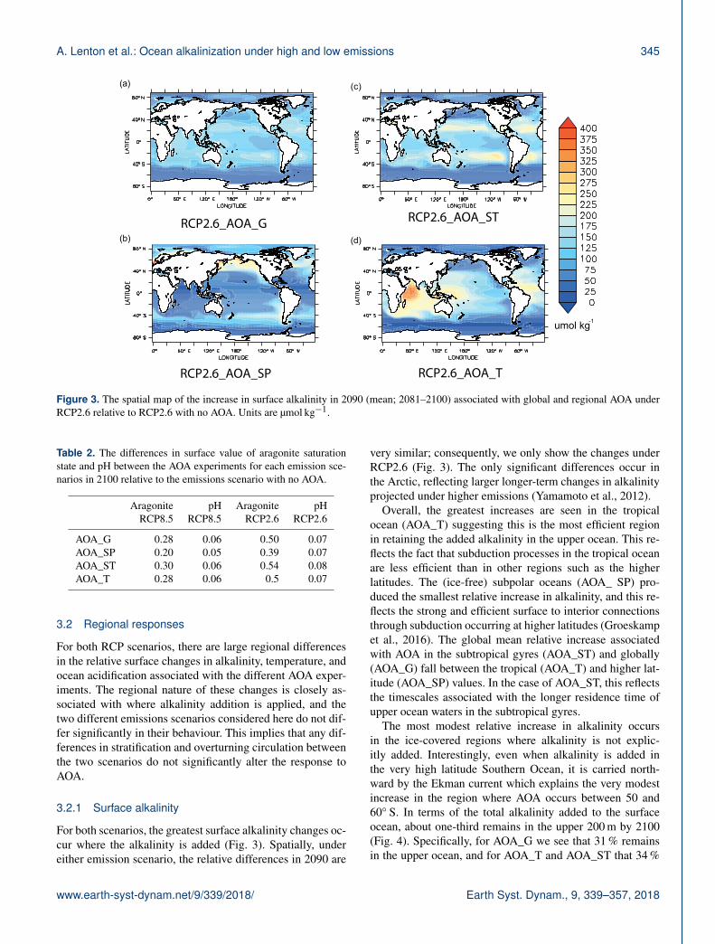
Figure 3. The spatial map of the increase in surface alkalinity in 2090 (mean; 2081–2100) associated with global and regional AOA underRCP2.6 relative to RCP2.6 with no AOA. Units are µmol kg−1.

Table 2. The differences in surface value of aragonite saturationstate and pH between the AOA experiments for each emission sce-narios in 2100 relative to the emissions scenario with no AOA.

Aragonite pH Aragonite pHRCP8.5 RCP8.5 RCP2.6 RCP2.6

AOA_G 0.28 0.06 0.50 0.07AOA_SP 0.20 0.05 0.39 0.07AOA_ST 0.30 0.06 0.54 0.08AOA_T 0.28 0.06 0.5 0.07

3.2 Regional responses

For both RCP scenarios, there are large regional differencesin the relative surface changes in alkalinity, temperature, andocean acidification associated with the different AOA exper-iments. The regional nature of these changes is closely as-sociated with where alkalinity addition is applied, and thetwo different emissions scenarios considered here do not dif-fer significantly in their behaviour. This implies that any dif-ferences in stratification and overturning circulation betweenthe two scenarios do not significantly alter the response toAOA.

3.2.1 Surface alkalinity

For both scenarios, the greatest surface alkalinity changes oc-cur where the alkalinity is added (Fig. 3). Spatially, undereither emission scenario, the relative differences in 2090 are

very similar; consequently, we only show the changes underRCP2.6 (Fig. 3). The only significant differences occur inthe Arctic, reflecting larger longer-term changes in alkalinityprojected under higher emissions (Yamamoto et al., 2012).

Overall, the greatest increases are seen in the tropicalocean (AOA_T) suggesting this is the most efficient regionin retaining the added alkalinity in the upper ocean. This re-flects the fact that subduction processes in the tropical oceanare less efficient than in other regions such as the higherlatitudes. The (ice-free) subpolar oceans (AOA_ SP) pro-duced the smallest relative increase in alkalinity, and this re-flects the strong and efficient surface to interior connectionsthrough subduction occurring at higher latitudes (Groeskampet al., 2016). The global mean relative increase associatedwith AOA in the subtropical gyres (AOA_ST) and globally(AOA_G) fall between the tropical (AOA_T) and higher lat-itude (AOA_SP) values. In the case of AOA_ST, this reflectsthe timescales associated with the longer residence time ofupper ocean waters in the subtropical gyres.

The most modest relative increase in alkalinity occursin the ice-covered regions where alkalinity is not explic-itly added. Interestingly, even when alkalinity is added inthe very high latitude Southern Ocean, it is carried north-ward by the Ekman current which explains the very modestincrease in the region where AOA occurs between 50 and60◦ S. In terms of the total alkalinity added to the surfaceocean, about one-third remains in the upper 200 m by 2100(Fig. 4). Specifically, for AOA_G we see that 31 % remainsin the upper ocean, and for AOA_T and AOA_ST that 34 %

www.earth-syst-dynam.net/9/339/2018/ Earth Syst. Dynam., 9, 339–357, 2018

346 A. Lenton et al.: Ocean alkalinization under high and low emissions

remains in the upper ocean, while for AOA_SP the figureis 22–24 % which (as anticipated) is lower than in other re-gions.

Spatially, AOA in the higher latitude regions (AOA_SP)leads to very large relative increases in alkalinity(> 1000 µmol kg−1; 2090) occurring along the northernmost boundary of the northern subpolar gyres, particularlythe North Pacific. Clearly, in this region the rate of AOAexceeds the rate of subduction allowing alkalinity to buildup. Large relative increases in alkalinity also occur in theSouthern Ocean under AOA_SP, particularly along westernboundary currents. However, in contrast to northern highlatitudes the values still remain low suggesting that the rateof addition does not exceed the rate of subduction evenunder the highest emission scenario.

AOA_ST shows a large relative increase of∼ 300 µmol kg−1 (2081–2100) in the subtropical gyreregions. Overall, we find that these relative increases arequite homogenous across the entire subtropical gyres, withstrong mixing with tropical waters leading to significantrelative increases in tropical Atlantic, western Pacific andIndian Oceans. Within the tropical ocean, under AOA_Tthe largest relative changes are found across the entiretropical Indian Ocean (∼ 400 µmol kg−1) with large relativeincreases also seen in the Indonesian seas (∼ 280 µmol kg−1;2081–2100). Away from the tropical Indian Ocean, we findthat relatively homogenous increases occur in the westernPacific and the Atlantic, with much more modest relativeincreases in the eastern Pacific reflecting the dominant eastto west upper ocean circulation. AOA_T leads to relativeincreases in surface alkalinity that are consistent with theresponse to AOA_ST – in the region of ∼ 130 µmol kg−1

(2081–2100).In the case of AOA_G, a relatively uniform net increase

in alkalinity occurs in all regions with the exception of theupwelling regions such as the tropical Pacific, which showeda more modest relative increase. In AOA_G there is little ev-idence of any of the very large increases in alkalinity seenin the more regional AOA experiments. This spatial patternof relative increase is broadly consistent with the pattern ofglobal alkalinity increase simulated by Ilyina et al. (2013)and Keller et al. (2014) for AOA in the (ice-free) globalocean.

3.2.2 Changes in the interior distribution of alkalinity inthe global ocean

As only about 30 % of the total AOA remains in the upper200 m, we explore the fate of this alkalinity in the interiorocean in the zonal sections of alkalinity (Fig. 4). As the pat-tern is very similar between RCP2.6 and RCP8.5, we onlyshow RCP2.6, noting that in the North Atlantic the projectedocean stratification is stronger under higher emissions (notshown) leading to slightly decreased subsurface values. This

increased stratification is consistent with other studies (e.g.Yool et al., 2015).

Unlike the surface plots of AOA, the relative increases insubsurface alkalinity due to AOA are very similar across allexperiments. This heterogeneous spatial pattern of alkalinityincrease is associated with water entering the interior oceanalong specific surface to interior pathways. Alkalinity alsomoves into the interior ocean along the poleward boundariesof the subtropical gyres, associated with the formation andsubduction of mode waters, and an increase in the subtropi-cal gyres associated with large-scale downwelling and deepmixing in the North Atlantic. The changes in alkalinity aremainly found in the upper ocean (< 1000 m) which reflectsthe relatively short period of alkalinity addition. Given theshort period, this is analogous to present-day observed distri-butions of anthropogenic carbon (Sabine et al., 2004).

As the changes in export production are very small, thelarge changes in the interior alkalinity concentrations pri-marily reflect the physical transport, rather than the sinkingand remineralization of calcium carbonate. Clearly other bi-ological processes, not represented in our model, have thepotential to impact the surface and interior values of alka-linity (Matear and Lenton, 2014). One such process is thereduction in the (rain) ratio of PIC : POC under higher emis-sions (Riebesell et al., 2000). However, it has been shownthat even a very large reduction in PIC production (50 %)would not significantly impact our results (Heinze, 2004).Unfortunately, at present the magnitude and sign of manyof these other feedbacks remain poorly known (Matear andLenton, 2014); consequently, quantifying their impact on ourresults is very difficult, and beyond the scope of this study.

3.2.3 Ocean carbon cycle response

The similarity in global ocean carbon uptake associated withall AOA experiments for a given emission scenario hides thelarge spatial differences between simulations. Given that thelargest carbon cycle response occurs in the ocean (Table 1),we focus on this response for RCP8.5 and RCP2.6 (Figs. 5and 6). As expected, ocean carbon uptake is strongly en-hanced in the regions of AOA. Away from regions of AOA,there is a reduction in carbon uptake, associated with theweakening of the gradient in CO2 between the atmosphereand ocean due to AOA. Interestingly, the largest increasespatially occurs in the Southern Ocean under AOA_SP forRCP2.6, while in contrast the largest changes under RCP8.5occur in the tropical ocean under AOA_T. The very smallchanges in export production in RCP2.6 were located in theArabian Sea (not shown), likely driven by enhanced mix-ing in this region. While these changes are < 1 % of the totalchange in carbon uptake, they may nevertheless be importantregionally.

Earth Syst. Dynam., 9, 339–357, 2018 www.earth-syst-dynam.net/9/339/2018/

A. Lenton et al.: Ocean alkalinization under high and low emissions 347

RCP2.6_AOA_SP

RCP2.6_AOA_G

RCP2.6_AOA_T

RCP2.6_AOA_ST

(a)

(b)

(c)

(d)

umol kg-1

Figure 4. The zonal mean changes in alkalinity in the interior ocean associated with global and regional AOA under RCP8.5 in 2090 (mean;2081–2100) relative to RCP8.5 with no AOA. Units are µmol kg−1.

gC m yr-2

RCP8.5_AOA_SP

RCP8.5_AOA_G

RCP8.5_AOA_T

RCP8.5_AOA_ST

(a)

(b)

(c)

(d)

-2

Figure 5. The spatial map of the changes in ocean carbon uptake in 2090 (mean; 2081–2100) associated with global and regional AOA underRCP8.5, relative to RCP8.5 with no AOA. Units are gC m−2 yr−1.

3.2.4 Temperature

The decrease in global mean SAT associated with all AOAexperiments for a given emission scenario again hides thelarge spatial differences between the simulations. The re-sponse of surface temperature is spatially very heterogeneous

(Figs. 7 and 8) and the regional surface temperature changesare very similar between the two emissions scenarios. Theexception to this is the Arctic which did not show a consistentresponse across the different AOA experiments, reflecting theperiod over which the mean changes were calculated, andthe simulated large variability in SAT in this region. Under

www.earth-syst-dynam.net/9/339/2018/ Earth Syst. Dynam., 9, 339–357, 2018

348 A. Lenton et al.: Ocean alkalinization under high and low emissions

RCP2.6_AOA_SP

RCP2.6_AOA_G

RCP2.6_AOA_T

RCP2.6_AOA_ST

(a)

(b)

(c)

(d)

gC m yr-2 -2

Figure 6. The spatial map of the changes in ocean carbon uptake in 2090 (mean; 2081–2100) associated with global and regional AOA underRCP2.6, relative to the RCP2.6 with no AOA. Units are gC m−2 yr−1.

RCP8.5_AOA_SP

RCP8.5_AOA_G

RCP8.5_AOA_T

RCP8.5_AOA_ST

K

(a)

(b)

(c)

(d)

Figure 7. The spatial map of the changes in surface air temperature 2090 (mean; 2081–2100) associated with global and regional AOA underRCP8.5, relative to RCP8.5 with no AOA. Units are K.

both emission scenarios, the largest cooling associated withAOA occurs over northern Russia and Canada, and Antarc-tica (greater than a −1.5 K cooling) with a larger cooling inthese regions under RCP2.6.

AOA in the RCP2.6 scenario brings about a net cooling ofthe surface ocean with the exception of the North Atlantic,east of New Zealand, and off the southern coast of Alaska,which show a very modest warming. A similar pattern is ev-

Earth Syst. Dynam., 9, 339–357, 2018 www.earth-syst-dynam.net/9/339/2018/

A. Lenton et al.: Ocean alkalinization under high and low emissions 349

RCP2.6_AOA_SP

RCP2.6_AOA_G

RCP2.6_AOA_T

K

RCP2.6_AOA_ST

(a)

(b)

(c)

(d)

Figure 8. The spatial map of the changes in surface air temperature 2090 (mean; 2081–2100) associated with global and regional AOA underRCP2.6, relative to the RCP2.6 with no AOA. Units are K.

pH

RCP8.5_AOA_SP

RCP8.5_AOA_G

RCP8.5_AOA_T

RCP8.5_AOA_ST

(a)

(b)

(c)

(d)

Figure 9. The spatial map of the changes in pH in 2090 (mean; 2081–2100) associated with global and regional AOA under RCP8.5, relativeto RCP8.5 with no AOA.

www.earth-syst-dynam.net/9/339/2018/ Earth Syst. Dynam., 9, 339–357, 2018

350 A. Lenton et al.: Ocean alkalinization under high and low emissions

RCP8.5_AOA_SP

RCP8.5_AOA_G

RCP8.5_AOA_T

RCP8.5_AOA_ST

(a)

(b)

(c)

(d)

Figure 10. The spatial map of the differences in surface aragonite saturation state in 2090 (mean; 2081–2100), associated with global andregional AOA under RCP8.5, relative to RCP8.5 with no AOA. Contoured on each map are the values of aragonite saturation state of 1 and3; please see the text for more explanation. The red contours represent RCP8.5 without AOA and the black contours represent RCP8.5 withAOA for each experiment.

ident in RCP8.5; however, there is a greater cooling in thehigh latitudes, and less cooling in the lower latitudes thanunder RCP2.6.

3.2.5 Ocean acidification response

Globally, the response of pH and aragonite saturation stateassociated with AOA are similar; however, large spatial andregional differences are present (Figs. 9–14). To aid in theinterpretation of changes in aragonite saturation state, over-lain on the aragonite saturation state maps are the contourscorresponding to the value of 3 – the approximate thresholdfor suitable coral habitat (Hoegh-Guldberg et al., 2007). Onthese surface maps and subsequent section plots we plot thesaturation horizon, i.e. the contour corresponding to the tran-sition from chemically stable to unstable (or corrosive), i.e.aragonite saturation state is equal to 1 (Orr et al., 2005).

The largest relative changes in pH and aragonite saturationstate were associated with regions of AOA (Figs. 9–12), re-flecting increases in the surface values of alkalinity (Fig. 3).All simulations increase pH and aragonite saturation state inthe Arctic despite no direct addition in this region, with thelargest changes here associated with AOA_G and AOA_SP.Interestingly, all simulations show little to no increase in thehigh latitude Southern Ocean, consistent with more efficienttransport of the added alkalinity into the ocean interior.

The changes in pH associated with AOA experiments un-der RCP8.5, while spatially very different particularly when

added in the subpolar ocean, are still much less than thedecreases associated with RCP8.5 with no AOA (Fig. 9).In terms of aragonite saturation state (Fig. 10), the condi-tions for coral growth in the tropical ocean remain very un-favourable by the end of century (i.e. aragonite saturationstate < 3) under all regional and global experiments, with theexception of AOA_T, where a very small region in the centralPacific Ocean exhibits suitable conditions.

Consistent with Feng et al. (2016), we find that this levelof AOA under RCP8.5 is insufficient to ameliorate or signif-icantly alter the large-scale changes in ocean acidification.More positively, at the higher latitudes the saturation hori-zon is moved poleward with the largest shift associated withAOA_SP, and the smallest shift at the high latitudes occur-ring under AOA_T. Consistent with these changes, we seea deepening of the saturation horizon everywhere, and lit-tle difference spatially between AOA experiments, consistentwith zonal mean changes in alkalinity for the four AOA ex-periments (Fig. 11).

The spatial pattern of changes associated with AOA un-der RCP2.6 is broadly consistent with that seen under higheremissions; however, the magnitude of the response is muchlarger – again, due to the larger differences between Alka-linity and DIC with AOA under RCP2.6 (Figs. 12 and 13).In terms of aragonite saturation state, the area of tropicalocean favourable for corals is considerably expanded. As an-ticipated the largest changes in the area favourable for trop-ical corals is associated with AOA_T, closely followed by

Earth Syst. Dynam., 9, 339–357, 2018 www.earth-syst-dynam.net/9/339/2018/

A. Lenton et al.: Ocean alkalinization under high and low emissions 351

RCP8.5_AOA_SP

RCP8.5_AOA_G

RCP8.5_AOA_T

RCP8.5_AOA_ST

(a)

(b)

(c)

(d)

Figure 11. The zonal mean differences in aragonite saturation state in 2090 (mean; 2081–2100), associated with global and regional AOAunder RCP8.5, relative to RCP8.5 with no AOA. Contoured on each map are the values of aragonite saturation state of 1; please see thetext for more explanation. The red contours represent RCP8.5 without AOA and the black contours represent RCP8.5 with AOA for eachexperiment.

AOA_ST. As the saturation horizon does not reach the sur-face under RCP2.6, we can only look at the changes in the in-terior ocean. Here, there is a deepening in the saturation hori-zon of a very similar magnitude in all experiments (Fig. 14),with the exception of the Arctic. Here, the response of the sat-uration horizon is more sensitive to the location of the AOA,varying between ∼ 100 m under AOA_T and ∼ 280 m underAOA_SP (Fig. 14).

Spatially, the large changes in ocean acidification in re-sponse to AOA under RCP2.6 more than compensate for thechanges in ocean chemistry due to low emissions in the pe-riod 2020–2100. Globally, the changes in the period 2020–2100 are sufficient to reverse or compensate for the changessince the pre-industrial period (1850). However, spatially insome regions such as equatorial upwelling, an important areaof global fisheries (Chavez et al., 2003), AOA in fact leads tohigher values of aragonite saturation state and pH than theocean experienced in the pre-industrial period (Feely et al.,2009). We can only speculate on the potential impact of areduction in aqueous CO2 and elevated pH levels on marinebiota in these regions. For a recent review of the potentialimpact of rising pH and aragonite saturation state on ma-rine organisms, we direct the reader to Renforth and Hen-derson (2017).

3.2.6 Importance of seasonality

In this paper, while we have focused on year-round AOA,as a sensitivity experiment we also explored whether AOAadded in summer or winter was more efficient. To do this,we focused on the higher latitudes regions where the largestseasonal changes in mixing are found (de Boyer Montegutet al., 2004; Trull et al., 2001). Here, we tested whetherAOA in either summer or winter was more effective thanyear-round addition. To test this for RCP8.5, we add alka-linity only during the summer at half of the annual rate (or0.125 PmolALK yr−1) in the AOA_SP region.

Our results showed that the response to AOA in summerwas very close to 50 % of the response of the year-roundaddition associated with AOA_SP (or 0.25 PmolALK yr−1).This suggests that the response of AOA appears invariantwith regard to when the alkalinity is added. This also sug-gests, consistent with published studies (e.g. Keller et al.,2014; Feng et al., 2016; Kohler et al., 2013), that the responseof the ocean to different quantities of AOA is scalable underthe same emissions scenario. Whether this is true under verymuch larger additions of alkalinity, as simulated by Gonzalezand Ilyina (2016), is less clear.

www.earth-syst-dynam.net/9/339/2018/ Earth Syst. Dynam., 9, 339–357, 2018

352 A. Lenton et al.: Ocean alkalinization under high and low emissions

pH

RCP2.6_AOA_SP

RCP2.6_AOA_G

RCP2.6_AOA_T

RCP2.6_AOA_ST

(a)

(b)

(c)

(d)

Figure 12. The spatial map of the changes in pH in 2090 (mean; 2081–2100) associated with global and regional AOA under RCP2.6,relative to RCP2.6 with no AOA.

RCP2.6_AOA_SP

RCP2.6_AOA_G

RCP2.6_AOA_T

RCP2.6_AOA_ST

(a)

(b)

(c)

(d)

Figure 13. The spatial map of the differences in surface aragonite saturation state in 2090 (mean; 2081–2100), associated with global andregional AOA under RCP2.6, relative to RCP2.6 with no AOA. Contoured on each map are the values of aragonite saturation state of 1 and3; please see the text for more explanation. The red contours represent RCP2.6 without AOA and the black contours represent RCP2.6 withAOA for each experiment.

Earth Syst. Dynam., 9, 339–357, 2018 www.earth-syst-dynam.net/9/339/2018/

A. Lenton et al.: Ocean alkalinization under high and low emissions 353

RCP2.6_AOA_SP

RCP2.6_AOA_G

RCP2.6_AOA_T

RCP2.6_AOA_ST

(a)

(b)

(c)

(d)

Figure 14. The zonal mean differences in aragonite saturation state in 2090 (mean; 2081–2100), associated with global and regional AOAunder RCP2.6, relative to RCP2.6 with no AOA. Contoured on each map are the values of aragonite saturation state of 1; please see thetext for more explanation. The red contours represent RCP2.6 without AOA and the black contours represent RCP2.6 with AOA for eachexperiment.

4 Summary and concluding remarks

Integrated Assessment modelling for the IntergovernmentalPanel on Climate Change shows that CO2 removal (CDR)may be required to achieve the goal of limiting warming towell below 2 ◦C (Fuss et al., 2014). Of the many schemes thathave been proposed to limit warming, only artificial ocean al-kalinization (AOA) is capable of both reducing the rate andmagnitude of global warming through reducing atmosphericCO2 concentrations, while simultaneously directly address-ing ocean acidification. Ocean acidification, while often re-ceiving less attention, is likely to have very long lasting anddamaging impacts on the entire marine ecosystem, and theecosystem services it provides.

Here, for the first time, we investigate the response ofa fully coupled climate ESM (i.e. one that accounts forclimate–carbon feedbacks) to a fixed addition of alkalin-ity (0.25 PmolALK yr−1) under high (RCP8.5) and low(RCP2.6) emissions scenarios. We explore the effect ofglobal and regional application of AOA focusing on the sub-polar gyres, the subtropical gyres and the tropical ocean. Toassess AOA, we look at changes in surface air temperature,carbon cycling, and ocean acidification (aragonite saturationstate and pH) in the period 2020–2100.

Consistent with other published studies, we see that AOAleads to reduced atmospheric CO2 concentrations, coolerglobal mean surface temperatures, and reduced levels ofocean acidification. Globally, for these metrics we observed

that they do not vary significantly between the various AOAexperiments under each emissions scenario. This implies thatat the global scale there is little sensitivity of the global re-sponses to the region where AOA is applied. We also investi-gate as a sensitivity experiment adding alkalinity in differentseasons and see little difference in response to when AOAwas undertaken.

We see under AOA that the increased carbon uptake isdominated by the ocean. Under RCP8.5, the changes due toAOA are only capable of reducing atmospheric concentra-tions by 16 % and, as such, the response of the climate systemremains strongly dominated by warming. This is consistentwith published studies of the response of the climate systemunder RCP8.5, and studies that have estimated the amount ofAOA required to counteract a high emissions trajectory.

In contrast, AOA under RCP2.6 – while only capable ofreducing atmospheric CO2 levels by 58 ppm – is sufficientto reduce atmospheric CO2 concentrations and warming toclose to 2020 levels at the end of the century. This is signifi-cant as it suggests that, in combination with a rapid reductionin emissions, AOA could make an important contribution tothe goal of keeping the rise in global mean temperatures be-low 2◦. However, AOA under the RCP2.6 emissions scenariochanges the roles played by the ocean and land in carbon up-take as compared with the scenario of RCP2.6 with no AOA,resulting in a reduced uptake in the terrestrial biosphere andincreased uptake in the ocean. This highlights that, while theatmospheric CO2 and warming may be reversible, the re-

www.earth-syst-dynam.net/9/339/2018/ Earth Syst. Dynam., 9, 339–357, 2018

354 A. Lenton et al.: Ocean alkalinization under high and low emissions

sponse of individual components of the Earth system to dif-ferent CDR may not be (Lenton et al., 2017).

Despite the impact of AOA on the atmospheric CO2 con-centration under RCP2.6 being only ∼ 60 % of the impactunder RCP8.5, we see much larger changes in ocean acid-ification associated with RCP2.6 than RCP8.5 – more than1.3 times in pH and more than 1.7 times in aragonite satu-ration state. This reflects the larger reductions in the differ-ence between ALK and DIC that occurs under RCP2.6. Wealso see larger relative decreases in global temperature asso-ciated with RCP2.6. These results are very important as theydemonstrate that AOA is more effective in reducing oceanacidification and global warming under lower emissions.

While there is little sensitivity in the global responses tothe region in which AOA is applied, spatially the largestchanges in ocean acidification (and ocean carbon uptake)were seen in the regions where AOA was applied. Despitelarge changes regionally, these cannot compensate for thelarge changes associated with RCP8.5. Even targeted AOA inthe tropical ocean can preserve only a tiny area of the oceanconducive to healthy coral growth; and even then the con-comitant large warming is likely to be a stronger influenceon coral growth than ocean chemistry (D’Olivo and McCul-loch, 2017).

In contrast, AOA under RCP2.6 is more than capable ofameliorating the projected ocean acidification changes in theperiod 2020–2100. We see that, in all cases, the area of thetropical ocean suitable for healthy coral growth expands,with the largest changes associated with tropical addition(AOA_T). In some areas, such as the equatorial Pacific, thechanges that have occurred since the pre-industrial period arealso completely reversed, and in some cases, lead to highervalues of aragonite saturation state and pH than were experi-enced in the pre-industrial period.

While the amount of alkalinity added in this study is smallin comparison to other published studies, the challenge ofachieving even this level of AOA should not be underes-timated. Indeed, it is not clear whether such an effort iseven feasible given the cost and the logistical, political, andengineering challenges of producing and distributing suchlarge quantities of alkaline material (Renforth and Hender-son, 2017). In the case of RCP8.5, it is unlikely that this levelof AOA could be justified given our results. If emissions canbe reduced along an RCP2.6 type trajectory, this study sug-gests that AOA is much more effective and may provide amethod to remove atmospheric CO2 to complement mitiga-tion, albeit with some side-effects, and may be an alternativeto reliance on land-based CDR.

In this work, and other published studies to date, we havenot accounted for the role of the mesoscale in AOA. In thereal ocean (mesoscale), eddies are ubiquitous and associatedwith strong convergent and divergent flows, and mixing playsan important role in ocean transport (Zhang et al., 2014). Itis plausible that the mesoscale, and indeed fine-scale circula-tion in the coastal environment (e.g. Mongin et al., 2016a, b),

may modulate the local response to AOA and this thereforeneeds to be considered in future studies.

Furthermore, this is a single model study, and the re-sults of this work need to be tested and compared in othermodels. The Carbon Dioxide Removal Model Intercompar-ison Project (CDRMIP) was created to coordinate and ad-vance the understanding of CDR in the Earth system (Lentonet al., 2017). CDRMIP brings together Earth system mod-els of varying complexity in a series of coordinated multi-model experiments, one of which is a global AOA experi-ment (CDR_4) (Keller et al., 2018). This will allow the re-sponse of the Earth system to AOA to be further exploredand quantified in a robust multi-model framework, and willexamine important further questions such as including cessa-tion effects of alkalinity addition, and the long-term fate ofadditional alkalinity in the ocean. In parallel, more processand observational studies (e.g. mesocosm experiments) areneeded to better understand the implications of AOA.

Data availability. The model code, simulations and scripts usedin this study are available by contacting Andrew Lenton(andrew.lenton@csiro.au) and a persistent URL on the CSIRO dataportal site https://data.csiro.au/dap will be created.

Competing interests. The authors declare that they have no con-flict of interest.

Acknowledgements. David P. Keller acknowledges fundingreceived from the German Research Foundation’s Priority Program1689 “Climate Engineering” (project CDR-MIA; KE 2149/2-1).The authors also wish to thank Tom W. Trull and the threeanonymous reviewers for their helpful comments that improvedthis manuscript.

Edited by: Ben KravitzReviewed by: three anonymous referees

References

Albright, R., Caldeira, L., Hosfelt, J., Kwiatkowski, L., Maclaren,J. K., Mason, B. M., Nebuchina, Y., Ninokawa, A., Pongratz, J.,Ricke, K. L., Rivlin, T., Schneider, K., Sesboue, M., Shamberger,K., Silverman, J., Wolfe, K., Zhu, K., and Caldeira, K.: Reversalof ocean acidification enhances net coral reef calcification, Na-ture, 531, 362–265, https://doi.org/10.1038/nature17155, 2016.

Best, M. J., Abramowitz, G., Johnson, H. R., Pitman, A. J., Bal-samo, G., Boone, A., Cuntz, M., Decharme, B., Dirmeyer, P.A., Dong, J., Ek, M., Guo, Z., Haverd, V., Van den Hurk, B. J.J., Nearing, G. S., Pak, B., Peters-Lidard, C., Santanello, J. A.,Stevens, L., and Vuichard, N.: The Plumbing of Land SurfaceModels: Benchmarking Model Performance, J. Hydrometeo-rol., 16, 1425–1442, https://doi.org/10.1175/JHM-D-14-0158.1,2015.

Earth Syst. Dynam., 9, 339–357, 2018 www.earth-syst-dynam.net/9/339/2018/

A. Lenton et al.: Ocean alkalinization under high and low emissions 355

Chavez, F. P., Ryan, J., Lluch-Cota, S. E., and Niquen,M.: From anchovies to sardines and back: Multidecadalchange in the Pacific Ocean, Science, 299, 217–221,https://doi.org/10.1126/Science.1075880, 2003.

Colbourn, G., Ridgwell, A., and Lenton, T. M.: The timescale of the silicate weathering negative feedback on at-mospheric CO2, Global Biogeochem. Cy., 29, 583–596,https://doi.org/10.1002/2014GB005054, 2015.

de Boyer Montegut, C., Madec, G., Fischer, A. S., Lazar,A., and Iudicone, D.: Mixed layer depth over the globalocean: An examination of profile data and a profile-based climatology, J. Geophys. Res.-Oceans, 109, C12003,https://doi.org/10.1029/2004jc002378, 2004.

D’Olivo, J. P. and McCulloch, M. T.: Response of coral cal-cification and calcifying fluid composition to thermallyinduced bleaching stress, Scientific Reports, 7, 2207,https://doi.org/10.1038/S41598-017-02306-X, 2017.

Doney, S. C., Ruckelshaus, M., Duffy, J. E., Barry, J. P., Chan,F., English, C. A., Galindo, H. M., Grebmeier, J. M., Hol-lowed, A. B., Knowlton, N., Polovina, J., Rabalais, N. N.,Sydeman, W. J., and Talley, L. D.: Climate Change Im-pacts on Marine Ecosystems, Annu. Rev. Mar. Sci., 4, 11–37,https://doi.org/10.1146/Annurev-Marine-041911-111611, 2012.

Duteil, O., Koeve, W., Oschlies, A., Aumont, O., Bianchi, D.,Bopp, L., Galbraith, E., Matear, R., Moore, J. K., Sarmiento,J. L., and Segschneider, J.: Preformed and regenerated phos-phate in ocean general circulation models: can right to-tal concentrations be wrong?, Biogeosciences, 9, 1797–1807,https://doi.org/10.5194/bg-9-1797-2012, 2012.

Fabry, V. J., Seibel, B. A., Feely, R. A., and Orr, J.C.: Impacts of ocean acidification on marine fauna andecosystem processes, ICES J. Mar. Sci., 65, 414–432,https://doi.org/10.1093/Icesjms/Fsn048, 2008.

Feely, R. A., Doney, S. C., and Cooley, S. R.: OceanAcidification: Present Conditions and Future Changesin a High-CO2 World, Oceanography, 22, 36–47,https://doi.org/10.5670/Oceanog.2009.95, 2009.

Feng, E. Y., Keller, D. P., Koeve, W., and Oschlies, A.: Couldartificial ocean alkalinization protect tropical coral ecosystemsfrom ocean acidification?, Environ. Res. Lett., 11, 074008,https://doi.org/10.1088/1748-9326/11/7/074008, 2016.

Feng, E. Y., Koeve, W., Keller, D. P., and Oschlies, A, Model-Based Assessment of the CO2 Sequestration Potential ofCoastal Ocean Alkalinization, Earth’s Future, 5, 1252–1266,https://doi.org/10.1002/2017EF000659, 2017.

Frolicher, T. L. and Joos, F.: Reversible and irreversible impactsof greenhouse gas emissions in multi-century projections withthe NCAR global coupled carbon cycle-climate model, Clim.Dynam., 35, 1439–1459, https://doi.org/10.1007/S00382-009-0727-0, 2010.

Fuss, S., Canadell, J. G., Peters, G. P., Tavoni, M., Andrew, R. M.,Ciais, P., Jackson, R. B., Jones, C. D., Kraxner, F., Nakicenovic,N., Le Quere, C., Raupach, M. R., Sharifi, A., Smith, P., and Ya-magata, Y.: Commentary: Betting on Negative Emissions, NatureClimate Change, 4, 850–853, 2014.

Gasser, T., Guivarch, C., Tachiiri, K., Jones, C. D., andCiais, P.: Negative emissions physically needed to keepglobal warming below 2 ◦C, Nat. Commun., 6, 7958,https://doi.org/10.1038/Ncomms8958, 2015.

Gattuso, J.-P., Magnan, A., Billé, R., Cheung, W. W. L., Howes, E.L., Joos, F., Allemand, D., Bopp, L., Cooley, S. R., Eakin, C.M., Hoegh-Guldberg, O., Kelly, R. P., Pörtner, H.-O., Rogers,A. D., Baxter, J. M., Laffoley, D., Osborn, D., Rankovic,A., Rochette, J., Sumaila, U. R., Treyer, S., and Turley, C.:Contrasting futures for ocean and society from different an-thropogenic CO2 emissions scenarios, Science, 349, aac4722,https://doi.org/10.1126/science.aac4722, 2015.

Gonzalez, M. F. and Ilyina, T.: Impacts of artificial oceanalkalinization on the carbon cycle and climate in Earthsystem simulations, Geophys. Res. Lett., 43, 6493–6502,https://doi.org/10.1002/2016GL068576, 2016.

Groeskamp, S., Lenton, A., Matear, R., Sloyan, B. M., andLanglais, C.: Anthropogenic carbon in the oceanSurface to in-terior connections, Global Biogeochem. Cy., 30, 1682–1698,https://doi.org/10.1002/2016GB005476, 2016.

Hauck, J., Kohler, P., Wolf-Gladrow, D., and Volker, C.: Ironfertilisation and century-scale effects of open ocean disso-lution of olivine in a simulated CO2 removal experiment,Environ. Res. Lett., 11, 024007, https://doi.org/10.1088/1748-9326/11/2/024007, 2016.

Heinze, C.: Simulating oceanic CaCO3 export productionin the greenhouse, Geophys. Res. Lett., 31, L16308,https://doi.org/10.1029/2004GL020613, 2004.

Hoegh-Guldberg, O., Mumby, P. J., Hooten, A. J., Steneck,R. S., Greenfield, P., Gomez, E., Harvell, C. D., Sale, P.F., Edwards, A. J., Caldeira, K., Knowlton, N., Eakin, C.M., Iglesias-Prieto, R., Muthiga, N., Bradbury, R. H., Dubi,A., and Hatziolos, M. E.: Coral reefs under rapid climatechange and ocean acidification, Science, 318, 1737–1742,https://doi.org/10.1126/science.1152509, 2007.

Hughes, T. P., Kerry, J. T., Alvarez-Noriega, M., Alvarez-Romero,J. G., Anderson, K. D., Baird, A. H., Babcock, R. C., Beger, M.,Bellwood, D. R., Berkelmans, R., Bridge, T. C., Butler, I. R.,Byrne, M., Cantin, N. E., Comeau, S., Connolly, S. R., Cumming,G. S., Dalton, S. J., Diaz-Pulido, G., Eakin, C. M., Figueira, W.F., Gilmour, J. P., Harrison, H. B., Heron, S. F., Hoey, A. S.,Hobbs, J. P. A., Hoogenboom, M. O., Kennedy, E. V., Kuo, C. Y.,Lough, J. M., Lowe, R. J., Liu, G., Cculloch, M. T. M., Malcolm,H. A., Mcwilliam, M. J., Pandolfi, J. M., Pears, R. J., Pratchett,M. S., Schoepf, V., Simpson, T., Skirving, W. J., Sommer, B.,Torda, G., Wachenfeld, D. R., Willis, B. L., and Wilson, S. K.:Global warming and recurrent mass bleaching of corals, Nature,543, 373–377, https://doi.org/10.1038/nature21707, 2017.

Iglesias-Rodriguez, M. D., Halloran, P. R., Rickaby, R. E. M.,Hall, I. R., Colmenero-Hidalgo, E., Gittins, J. R., Green,D. R. H., Tyrrell, T., Gibbs, S. J., von Dassow, P., Rehm,E., Armbrust, E. V., and Boessenkool, K. P.: Phytoplanktoncalcification in a high-CO2 world, Science, 320, 336–340,https://doi.org/10.1126/Science.1154122, 2008.

Ilyina, T., Wolf-Gladrow, D., Munhoven, G., and Heinze, C.:Assessing the potential of calcium-based artificial oceanalkalinization to mitigate rising atmospheric CO2 andocean acidification, Geophys. Res. Lett., 40, 5909–5914,https://doi.org/10.1002/2013GL057981, 2013.

Jickells, T. D., An, Z. S., Andersen, K. K., Baker, A. R., Berga-metti, G., Brooks, N., Cao, J. J., Boyd, P. W., Duce, R. A.,Hunter, K. A., Kawahata, H., Kubilay, N., laRoche, J., Liss,P. S., Mahowald, N., Prospero, J. M., Ridgwell, A. J., Tegen,

www.earth-syst-dynam.net/9/339/2018/ Earth Syst. Dynam., 9, 339–357, 2018

356 A. Lenton et al.: Ocean alkalinization under high and low emissions

I., and Torres, R.: Global iron connections between desertdust, ocean biogeochemistry, and climate, Science, 308, 67–71,https://doi.org/10.1126/Science.1105959, 2005.

Jones, C. D., Arora, V., Friedlingstein, P., Bopp, L., Brovkin, V.,Dunne, J., Graven, H., Hoffman, F., Ilyina, T., John, J. G.,Jung, M., Kawamiya, M., Koven, C., Pongratz, J., Raddatz,T., Randerson, J. T., and Zaehle, S.: C4MIP – The CoupledClimate–Carbon Cycle Model Intercomparison Project: experi-mental protocol for CMIP6, Geosci. Model Dev., 9, 2853–2880,https://doi.org/10.5194/gmd-9-2853-2016, 2016.

Keller, D. P., Feng, E. Y., and Oschlies, A.: Potential cli-mate engineering effectiveness and side effects during a highcarbon dioxide-emission scenario, Nat. Commun., 5, 3304,https://doi.org/10.1038/Ncomms4304, 2014.

Keller, D. P., Lenton, A., Scott, V., Vaughan, N. E., Bauer, N., Ji,D., Jones, C. D., Kravitz, B., Muri, H., and Zickfeld, K.: TheCarbon Dioxide Removal Model Intercomparison Project (CDR-MIP): rationale and experimental protocol for CMIP6, Geosci.Model Dev., 11, 1133–1160, https://doi.org/10.5194/gmd-11-1133-2018, 2018.

Kheshgi, H. S.: Sequestering Atmospheric Carbon-Dioxideby Increasing Ocean Alkalinity, Energy, 20, 915–922,https://doi.org/10.1016/0360-5442(95)00035-F, 1995.

Kohler, P., Abrams, J. F., Volker, C., Hauck, J., and Wolf-Gladrow,D. A.: Geoengineering impact of open ocean dissolution ofolivine on atmospheric CO2, surface ocean pH and marinebiology, Environ. Res. Lett., 8, https://doi.org/10.1088/1748-9326/8/1/014009, 2013.

Krasting, J. P., Dunne, J. P., Shevliakova, E., and Stouffer, R. J.:Trajectory sensitivity of the transient climate response to cumu-lative carbon emissions, Geophys. Res. Lett., 41, 2520–2527,https://doi.org/10.1002/2013gl059141, 2014.

Lenton, A. and Matear, R. J.: Role of the Southern Annular Mode(SAM) in Southern Ocean CO2 uptake, Global Biogeochem. Cy.,21, https://doi.org/10.1029/2006GB002714, 2007.

Lenton, A., Tilbrook, B., Matear, R. J., Sasse, T. P., andNojiri, Y.: Historical reconstruction of ocean acidificationin the Australian region, Biogeosciences, 13, 1753–1765,https://doi.org/10.5194/bg-13-1753-2016, 2016.

Lenton, A., Keller, D. P., and Pfister, P.: How Will Earth Re-spond to Plans for Carbon Dioxide Removal?, EOS, 98,https://doi.org/10.1029/2017EO068385, 2017.

Le Quéré, C., Moriarty, R., Andrew, R. M., Peters, G. P., Ciais, P.,Friedlingstein, P., Jones, S. D., Sitch, S., Tans, P., Arneth, A.,Boden, T. A., Bopp, L., Bozec, Y., Canadell, J. G., Chini, L. P.,Chevallier, F., Cosca, C. E., Harris, I., Hoppema, M., Houghton,R. A., House, J. I., Jain, A. K., Johannessen, T., Kato, E., Keel-ing, R. F., Kitidis, V., Klein Goldewijk, K., Koven, C., Landa,C. S., Landschützer, P., Lenton, A., Lima, I. D., Marland, G.,Mathis, J. T., Metzl, N., Nojiri, Y., Olsen, A., Ono, T., Peng, S.,Peters, W., Pfeil, B., Poulter, B., Raupach, M. R., Regnier, P., Rö-denbeck, C., Saito, S., Salisbury, J. E., Schuster, U., Schwinger,J., Séférian, R., Segschneider, J., Steinhoff, T., Stocker, B. D.,Sutton, A. J., Takahashi, T., Tilbrook, B., van der Werf, G. R.,Viovy, N., Wang, Y.-P., Wanninkhof, R., Wiltshire, A., and Zeng,N.: Global carbon budget 2014, Earth Syst. Sci. Data, 7, 47–85,https://doi.org/10.5194/essd-7-47-2015, 2015.

Lovelock, J. E. and Rapley, C. G.: Ocean pipes couldhelp the Earth to cure itself, Nature, 449, 403–403,https://doi.org/10.1038/449403a, 2007.

Lovenduski, N. S., Long, M. C., and Lindsay, K.: Natural variabil-ity in the surface ocean carbonate ion concentration, Biogeo-sciences, 12, 6321–6335, https://doi.org/10.5194/bg-12-6321-2015, 2015.

Mao, J., Phipps, S. J., Pitman, A. J., Wang, Y. P., Abramowitz,G., and Pak, B.: The CSIRO Mk3L climate system model v1.0coupled to the CABLE land surface scheme v1.4b: evaluationof the control climatology, Geosci. Model Dev., 4, 1115–1131,https://doi.org/10.5194/gmd-4-1115-2011, 2011.

Matear, R. J. and Hirst, A. C.: Long term changes in dis-solved oxygen concentrations in the ocean caused by pro-tracted global warming, Global Biogeochem. Cy., 17, 1125,https://doi.org/10.1029/2002GB001997, 2003.

Matear, R. J. and Lenton, A.: Quantifying the impact of ocean acid-ification on our future climate, Biogeosciences, 11, 3965–3983,https://doi.org/10.5194/bg-11-3965-2014, 2014.

Mathesius, S., Hofmann, M., Caldeira, K., and Schellnhu-ber, H. J.: Long-term response of oceans to CO2 removalfrom the atmosphere, Nature Climate Change, 5, 1107–1113,https://doi.org/10.1038/NCLIMATE2729, 2015.

Mongin, M., Baird, M. E., Hadley, S., and Lenton, A.: Optimisingreef-scale CO2 removal by seaweed to buffer ocean acidification,Environ. Res. Lett., 11, 034023, https://doi.org/10.1088/1748-9326/11/3/034023, 2016a.

Mongin, M., Baird, M. E., Tilbrook, B., Matear, R. J., Lenton,A., Herzfeld, M., Wild-Allen, K., Skerratt, J., Margvelashvili,N., Robson, B. J., Duarte, C. M., Gustafsson, M. S. M., Ralph,P. J., and Steven, A. D. L.: The exposure of the Great Bar-rier Reef to ocean acidification, Nat. Commun., 7, 10732,https://doi.org/10.1038/Ncomms10732, 2016b.

Montserrat, F., Renforth, P., Hartmann, J., Leermakers, M., Knops,P., and Meysman, F. J. R.: Olivine Dissolution in Seawater: Im-plications for CO2 Sequestration through Enhanced Weatheringin Coastal Environments, Environ. Sci. Technol., 51, 3960–3972,https://doi.org/10.1021/acs.est.6b05942, 2017.

Mucci, A.: The Solubility of Calcite and Aragonite in Seawaterat Various Salinities, Temperatures, and One Atmosphere TotalPressure, Am. J. Sci., 283, 780–799, 1983.

Munday, P. L., Donelson, J. M., Dixson, D. L., and Endo, G. G.K.: Effects of ocean acidification on the early life history of atropical marine fish, P. Roy. Soc. B-Biol. Sci., 276, 3275–3283,https://doi.org/10.1098/Rspb.2009.0784, 2009.

Munday, P. L., Dixson, D. L., McCormick, M. I., Meekan,M., Ferrari, M. C. O., and Chivers, D. P.: Replenish-ment of fish populations is threatened by ocean acid-ification, P. Natl. Acad. Sci. USA, 107, 12930–12934,https://doi.org/10.1073/Pnas.1004519107, 2010.

National Research Council: Climate Intervention: CarbonDioxide Removal and Reliable Sequestration, Washing-ton, DC, The National Academies Press, available at:https://doi.org/10.17226/18805 (last access: 3 April 2018),2015.

Orr, J. C., Fabry, V. J., Aumont, O., Bopp, L., Doney, S. C., Feely, R.A., Gnanadesikan, A., Gruber, N., Ishida, A., Joos, F., Key, R. M.,Lindsay, K., Maier-Reimer, E., Matear, R., Monfray, P., Mouchet,A., Najjar, R. G., Plattner, G. K., Rodgers, K. B., Sabine, C.

Earth Syst. Dynam., 9, 339–357, 2018 www.earth-syst-dynam.net/9/339/2018/

A. Lenton et al.: Ocean alkalinization under high and low emissions 357

L., Sarmiento, J. L., Schlitzer, R., Slater, R. D., Totterdell, I. J.,Weirig, M. F., Yamanaka, Y., and Yool, A.: Anthropogenic oceanacidification over the twenty-first century and its impact on cal-cifying organisms, Nature, 437, 681–686, 2005.

Phipps, S. J., Rotstayn, L. D., Gordon, H. B., Roberts, J. L.,Hirst, A. C., and Budd, W. F.: The CSIRO Mk3L climate sys-tem model version 1.0 – Part 2: Response to external forcings,Geosci. Model Dev., 5, 649–682, https://doi.org/10.5194/gmd-5-649-2012, 2012.

Ragueneau, O., Treguer, P., Leynaert, A., Anderson, R. F., Brzezin-ski, M. A., DeMaster, D. J., Dugdale, R. C., Dymond, J., Fischer,G., Francois, R., Heinze, C., Maier-Reimer, E., Martin-Jezequel,V., Nelson, D. M., and Queguiner, B.: A review of the Si cyclein the modem ocean: recent progress and missing gaps in the ap-plication of biogenic opal as a paleoproductivity proxy, GlobalPlanet. Change, 26, 317–365, https://doi.org/10.1016/S0921-8181(00)00052-7, 2000.

Raven, J., Caldeira, K., Elderfield, H., Hoegh-Guldberg, O., Liss,P., and Riebesell, U.: Ocean acidification due to increasing at-mospheric carbon dioxide, The Royal Society, Policy Document,London, UK, 2005.

Renforth, P. and Henderson, G.: Assessing ocean alkalin-ity for carbon sequestration, Rev. Geophys., 55, 636–674,https://doi.org/10.1002/2016RG000533, 2017.

Revelle, R. and Suess, H. E.: Carbon dioxide exchange betweenatmosphere and ocean and the question of an increase of atmo-spheric CO2 during the past decades, Tellus, 9, 18–27, 1957.

Riebesell, U., Zondervan, I., Rost, B., Tortell, P. D., Zeebe, R. E.,and Morel, F. M. M.: Reduced calcification of marine plankton inresponse to increased atmospheric CO2, Nature, 407, 364–367,2000.

Riebesell, U., Fabry, V. J., Hansson, L., and Gattuso, J.-P.: Guide tobest practices for ocean acidification research and data reporting,Publications Office of the European Union, Luxembourg, 260,2010.

Rogelj, J., den Elzen, M., Hohne, N., Fransen, T., Fekete, H.,Winkler, H., Chaeffer, R. S., Ha, F., Riahi, K., and Mein-shausen, M.: Paris Agreement climate proposals need a boostto keep warming well below 2 ◦C, Nature, 534, 631–639,https://doi.org/10.1038/nature18307, 2016.

Sabine, C. L., Feely, R. A., Gruber, N., Bullister, J. L., Wanninkhof,R., Wong, C. S., Wallace, D. W. R., Tilbrook, B., Millero, F. J.,Peng, T.-H., Kozyr, A., Ono, T., and Rios, A. F.: The OceanicSink for Anthropogenic CO2, Science, 305, 367–371, 2004.

Scott, V., Haszeldine, R. S., Tett, S. F. B., and Oschlies, A.: Fossilfuels in a trillion tonne world, Nature Climate Change, 5, 419–423, https://doi.org/10.1038/NCLIMATE2578, 2015.

Shepherd, J. G., Caldeira, K., Cox, P., Haigh, J., Keith, D., Launder,B. E., Mace, G., MacKerron, G., Pyle, J., Raynor, S., Redgwell,C., and Watson, A.: Geoengineering the Climate: Science, gov-ernance and uncertainty, London, The Royal Society Publishing,82 pp., 2009.

Sigman, D. M. and Boyle, E. A.: Glacial/interglacial varia-tions in atmospheric carbon dioxide, Nature, 407, 859–869,https://doi.org/10.1038/35038000, 2000.

Smith, P., Davis, S. J., Creutzig, F., Fuss, S., Minx, J., Gabrielle,B., Kato, E., Jackson, R. B., Cowie, A., Kriegler, E., van Vu-uren, D. P., Rogelj, J., Ciais, P., Milne, J., Canadell, J. G.,McCollum, D., Peters, G., Andrew, R., Krey, V., Shrestha, G.,Friedlingstein, P., Gasser, T., Grubler, A., Heidug, W. K., Jonas,M., Jones, C. D., Kraxner, F., Littleton, E., Lowe, J., Mor-eira, J. R., Nakicenovic, N., Obersteiner, M., Patwardhan, A.,Rogner, M., Rubin, E., Sharifi, A., Torvanger, A., Yamagata,Y., Edmonds, J., and Cho, Y.: Biophysical and economic limitsto negative CO2 emissions, Nature Climate Change, 6, 42–50,https://doi.org/10.1038/NCLIMATE2870, 2016.

Taylor, K. E., Stouffer, R. J., and Meehl, G. A.: An Overview ofCMIP5 and the Experiment Design, B. Am. Meteorol. Soc., 93,485–498, https://doi.org/10.1175/BAMS-D-11-00094.1, 2012.

Trull, T. W., Rintoul, S. R., Hadfield, M., and Abraham, E. R.: Cir-culation and seasonal evolution of polar waters south of Aus-tralia: Implications for iron fertilizations for the Southern Ocean,Deep-Sea Res. Pt. II, 48, 2439–2466, 2001.

United Nations Framework on Climate Change (UNFCCC): Adop-tion of the Paris Agreement, 21st Conference of the Parties, avail-able at: https://unfccc.int/resource/docs/2015/cop21/eng/l09r01.pdf (last access: 3 April 2018), 2015.

Wang, Y. P., Law, R. M., and Pak, B.: A global model of carbon,nitrogen and phosphorus cycles for the terrestrial biosphere, Bio-geosciences, 7, 2261–2282, https://doi.org/10.5194/bg-7-2261-2010, 2010.

Yamamoto, A., Kawamiya, M., Ishida, A., Yamanaka, Y., andWatanabe, S.: Impact of rapid sea-ice reduction in the ArcticOcean on the rate of ocean acidification, Biogeosciences, 9,2365–2375, https://doi.org/10.5194/bg-9-2365-2012, 2012.

Yamanaka, Y. and Tajika, E.: The role of vertical fluxes of par-ticulate organic material and calcite in the oceanic carbon cy-cle: Studies using a ocean biogeochemical general; circulationmodel, Global Biogeochem. Cy., 10, 361–382, 1996.

Yool, A., Popova, E. E., and Coward, A. C.: Futurechange in ocean productivity: Is the Arctic the newAtlantic?, J. Geophys. Res.-Oceans, 120, 7771–7790,https://doi.org/10.1002/2015JC011167, 2015.

Zeebe, R. E.: History of Seawater Carbonate Chemistry, Atmo-spheric CO2, and Ocean Acidification, Annu. Rev. Earth Pl.Sc., 40, 141–165, https://doi.org/10.1146/annurev-earth-042711-105521, 2012.

Zhang, Q., Wang, Y. P., Matear, R. J., Pitman, A. J., and Dai, Y.J.: Nitrogen and phosphorous limitations significantly reduce fu-ture allowable CO2 emissions, Geophys. Res. Lett., 41, 632–637,https://doi.org/10.1002/2013GL058352, 2014.

Zhang, Z. G., Wang, W., and Qiu, B.: Oceanic masstransport by mesoscale eddies, Science, 345, 322–324,https://doi.org/10.1126/science.1252418, 2014.

www.earth-syst-dynam.net/9/339/2018/ Earth Syst. Dynam., 9, 339–357, 2018