article in press - woods hole oceanographic institution · two challenges of laser raman...

Chemical Geology xxx (2008) xxx–xxx

CHEMGE-15589; No of Pages 13

Contents lists available at ScienceDirect

Chemical Geology

j ourna l homepage: www.e lsev ie r.com/ locate /chemgeo

ARTICLE IN PRESS

Laser Raman spectroscopy as a technique for identification of seafloor hydrothermaland cold seep minerals

Sheri N. White ⁎Department of Applied Ocean Physics and Engineering, Woods Hole Oceanographic Institution, Woods Hole, MA 02536, USA

⁎ Woods Hole Oceanographic Institution, Blake 209, MUSA. Tel.: +1 508 289 3740; fax: +1 508 457 2006.

E-mail address: [email protected].

0009-2541/$ – see front matter © 2008 Elsevier B.V. Aldoi:10.1016/j.chemgeo.2008.11.008

Please cite this article as: White, S.N., Laseminerals, Chem. Geol. (2008), doi:10.1016/j

a b s t r a c t
a r t i c l e i n f o
Article history:
In situ sensors capable of re Received 8 August 2008Received in revised form 8 November 2008Accepted 10 November 2008Available online xxxx
Editor: R.L. Rudnick

Keywords:Raman spectroscopyMineralogyHydrothermal ventsCold seepsSulfatesSulfides

al-time measurements and analyses in the deep ocean are necessary to fulfill thepotential created by the development of autonomous, deep-sea platforms such as autonomous and remotelyoperated vehicles, and cabled observatories. Laser Raman spectroscopy (a type of vibrational spectroscopy) is anoptical technique that is capable of in situmolecular identification of minerals in the deep ocean. The goals of thiswork are to determine the characteristic spectral bands and relative Raman scattering strength of hydrothermally-and cold seep-relevant minerals, and to determine how the quality of the spectra are affected by changes inexcitationwavelength and sampling optics. The information learned from this workwill lead to the developmentof new, smaller sea-going Raman instruments that are optimized to analyze minerals in the deep ocean.Manyminerals of interest at seafloor hydrothermal and cold seep sites are Raman active, such as elemental sulfur,carbonates, sulfates and sulfides. Elemental S8 sulfur is a strongRaman scattererwithdominant bands at∼219 and472 Δcm−1. The Raman spectra of carbonates (such as the polymorphs calcite and aragonite) are dominated byvibrations within the carbonate ion with a primary band at ∼1085 Δcm−1. The positions of minor Raman bandsdifferentiate these polymorphs. Likewise, the Raman spectra of sulfates (such as anhydrite, gypsumand barite) aredominated by the vibration of the sulfate ion with a primary band around 1000 Δcm−1 (∼1017 for anhydrite,∼1008 for gypsum, and ∼988 for barite). Sulfides (pyrite, marcasite, chalcopyrite, isocubanite, sphalerite, andwurtzite) are weaker Raman scatters than carbonate and sulfate minerals. They have distinctive Raman bands inthe ∼300–500 Δcm−1 region. Raman spectra from these mineral species are very consistent in band position andnormalized band intensity. High quality Raman spectra are obtained from all of these minerals using both greenand red excitation lasers, and using a variety of sampling optics. The highest quality spectra (highest signal-to-noise) were obtained using green excitation (532 nm Nd:YAG laser) and a sampling optic with a short depth offocus (and thus high power density). Significant fluorescence was not observed for the minerals analyzed usinggreen excitation.Spectra were also collected from pieces of active and inactive hydrothermal chimneys, recovered from the KiloMoana vent field in 2005 and 11°N on the East Pacific Rise in 1988, respectively. Profiles of sample J2-137-1-r1-ashow the transition from the chalcopyrite-rich “inner”wall to the sphalerite-dominated “outer”wall, and indicatethe presence of minor amounts of anhydrite. Spectra collected from sample A2003-7-1a5 identify Cu–S tarnishespresent on the surface of the sample.

© 2008 Elsevier B.V. All rights reserved.

1. Introduction

The future of oceanography is being shaped by the development ofnew underwater platforms that are autonomously or remotely oper-ated. These include remotely operated vehicles (ROVs), autonomousunderwater vehicles (AUVs), deep-sea moorings and seafloor cabledobservatories. These platforms are most efficient when equipped withinstruments capable of in situ measurements and analyses. That is,they are changing oceanography from a “sampling” science to a“sensing” science. Some oceanographic disciplines are already well

S#7, Woods Hole, MA 02543,

l rights reserved.

r Raman spectroscopy as a t.chemgeo.2008.11.008

suited to this new paradigm. The primary instrument of the physicaloceanographer is the CTD (Conductivity–Temperature–Depth sensor),and marine geophysicists routinely deploy magnetometers, gravime-ters, and seafloor seismometers. However, the disciplines of chem-istry, biology and geology are lagging in in situ technology (Varney,2000; Daly et al., 2004; Prien, 2007). Technologies are now becomingavailable that can identify the chemical composition of minerals insitu in the deep ocean.

1.1. Hydrothermal vents and cold seeps

One area in particular that would benefit from new sensing tech-nology is the study of seafloor hydrothermal and cold seep systems.Hydrothermal vents occur along seafloor spreading ridges throughout

echnique for identification of seafloor hydrothermal and cold seep

mailto:[email protected]

http://dx.doi.org/10.1016/j.chemgeo.2008.11.008

http://www.sciencedirect.com/science/journal/00092541


2 S.N. White / Chemical Geology xxx (2008) xxx–xxx

ARTICLE IN PRESS

the world ocean (Baker and German, 2004). Cold seawater circulateswithin recently formed, still hot crust, above a magma lens, where it isheated and reacts with the host rock. Modification of the fluid includesremoval of Mg, exchange of Ca for Na, and addition of metals andvolatiles (Alt, 1995). The modified fluid rises buoyantly to the surfacewhere it exits the seafloor as focused, high-temperature (∼350 °C)vents or lower-temperature (∼20 °C) diffuse flow. At highest-temperature vents, the hydrothermal fluid mixes with seawaterabove the vent orifice, resulting in precipitation of metal-bearingphases in the rising plume— thus receiving the name “black smokers.”Anhydrite- and sulfide-rich chimneys are formed at vent orifices, andthey evolve and mature (Goldfarb et al., 1983; Haymon, 1983). Hy-drothermal fluids and mineral deposits exhibit compositional ranges,based in part on the host rock (e.g., basalt, enriched mid-ocean ridgebasalt, andesite, rhyolite, peridotite, presence or absence of sediment),and in part on styles of mixing (e.g., Tivey, 1995; Hannington et al.,2005; Tivey, 2007). Hydrothermal vent fields are also home to uniquebiological communities that are supported by chemosyntheticbacteria and archaea (Hessler and Kaharl, 1995). Studying the varietyof minerals that are deposited and precipitated at hydrothermalvent sites can provide insights into those processes occurring in thesubsurface that affect ocean chemistry and the seafloor biologicalcommunities.

Cold seeps are sites where natural gas (primarily methane) ispercolating through the seafloor. These sites often occur alongcontinental margins, such as Hydrate Ridge off the coast of Oregon,where in some cases, gas bubbles are actively venting from the seafloor. At the proper pressure and temperature conditions, the gas andwater mix to form solid clathrate hydrates. Clathrate hydrate is an ice-like lattice that holds gasmolecules (e.g., carbon dioxide, methane andhigher hydrocarbons) in cages in the lattice structure. The gas-richfluids at these seep sites support chemosynthetic communities similarto those at hydrothermal vents — bacterial mats, clams, mussels, tubeworms, etc. (Sibuet and Olu, 1998). Carbonate crusts (which caninclude calcite and dolomite) are also known to form in cold seepregions (Aloisi et al., 2000, 2002; Luff et al., 2004).

1.2. Laser Raman spectroscopy in the ocean

Laser Raman spectroscopy (a type of vibrational spectroscopy) is anoptical technique, well suited to extreme environments, that is capableof in situ molecular identification of solids, liquids, and gases. Ramanspectroscopy is non-invasive, non-destructive and does not requirereagents or consumables. A laser excites a target, and the spectrumof theenergy-shifted, back-scattered radiation serves as a “fingerprint” —

providing compositional and structural information. The Ramanscattered photons can have lower or higher energies than the incidentphotons —Stokes and anti-Stokes scattering, respectively. In this paperwe look only at the Stokes (lower energy, higherwavelength) scattering.The spectrum is plotted as intensity vs. Raman shift in wavenumbers(Δcm−1), shifted from the absolute frequency (in cm−1) of the excitationlaser. A more detailed discussion of Raman theory can be found inFerraro et al. (2003) and Nakamoto (1997), and references therein.Raman spectroscopy has been used successfully for mineral identifica-tion in the laboratory (e.g., Haskin et al., 1997; Pasteris, 1998; Nasdalaet al., 2004) and is capable of distinguishing between mineral poly-morphs (e.g., calcite and aragonite, which are both CaCO3). Many rocksand minerals found in the deep ocean are Raman active. These includecomponents of basalt, and hydrothermal minerals such as anhydrite,sphalerite, chalcopyrite, and others. Raman spectroscopy is also wellsuited to making measurements in the ocean because water is a rel-atively weak Raman scatterer (Williams and Collette, 2001).

A sea-going Raman instrument (DORISS— Deep Ocean Raman In SituSpectrometer) has beendevelopedanddeployed at avariety of sites in thedeep ocean (Brewer et al., 2004; Pasteris et al., 2004). This system wasbuilt as a proof-of-conceptwith a broad spectral range (100–4400Δcm−1)

Please cite this article as: White, S.N., Laser Raman spectroscopy as a tminerals, Chem. Geol. (2008), doi:10.1016/j.chemgeo.2008.11.008

and thus is capable of analyzing a large variety of solids, liquids and gases.DORISS consists of a 532 nm Nd:YAG excitation laser and a laboratory-model spectrometer with a duplex holographic grating and a TE-cooledCCD camera. The green laserwas chosen for its high transmission throughwater. A remote optical head, connected to the laser and spectrometer viafiber optic cables, is capable of using a stand-off optic behind a pressurewindow with a working distance of up to 15 cm or an immersion opticwith a sapphire window and a 6 mm working distance (Brewer et al.,2004). DORISS has been used to identify and analyze gasmixtures (Whiteet al., 2006a), gas hydrates (Hester et al., 2006, 2007), and minerals.Naturally occurring minerals identified in situ by Raman spectroscopy todate include hydrothermally produced barite and anhydrite, calcite andaragonite in shells, and bacterially produced sulfur (White et al., 2005,2006b).

Although DORISS has been used successfully in the ocean, theinstrumentation, technique and data analysis methods have not beenfully explored and developed (optimized) for hydrothermal vent andcold seep applications. The current work builds on initial deploymentsof the DORISS instrument to identify seafloor minerals. The goals ofthis work are to determine the characteristic spectral bands andRaman scattering strength of hydrothermally- and cold seep-relevantminerals, and to determine how the quality of the spectra are affectedby changes in excitation wavelength and sampling optics. The infor-mation learned from this work will lead to the development of new,smaller sea-going Raman instruments that are optimized to analyzeminerals in the deep ocean.

2. Application of laser Raman spectroscopy to mineralogy

Raman spectroscopy has been applied to minerals (e.g., Landsbergand Mandelstam, 1928) since its discovery in 1928 (Raman andKrishnan, 1928). Recent reviews by Smith and Carabatos-Nédelec(2001) and Nasdala et al. (2004) provide thorough discussions of theapplication of Raman spectroscopy to minerals and crystals. It shouldbe noted that the Raman spectra of crystals are not as consistent as thespectra of gases and liquids. That is, the band positions and relativeband intensities may vary slightly from one spectrum to another dueto the orientation of the crystal lattice (and optical properties of thecrystal) and/or the presence of local impurities or irregularities in thecrystal structure. Typically, in the literature, band positions arereported, but not band intensity. Band intensity may be suggestedby identifying the primary bands, or by the indicators “w” (weak) “m”

(moderate) “s” (strong), or “vs” (very strong). In this paper, normalizedband intensities (i.e., the band height above background divided bythe height of the dominant band) and the range of those intensitieswill be reported to show how much variation in intensity one mayexpect to observe.

Raman spectroscopy is well suited to qualitative species identifica-tion. However, for quantitative analyses, Raman band heights in rawspectra cannot be used to straightforwardly infer concentration orabundance. This is due to the fact that different species have differentRaman scattering efficiencies. Additionally, for heterogeneous samples,the species abundance in the area of the of sample illuminated by thelaser spotmay not be characteristic of the entire sample. For well mixedsamples, suchas liquids andgases, ratio techniques canbeused to obtaininformation on relative concentration (e.g., Wopenka and Pasteris,1987). For solid species, point-counting techniques can be used todetermine relative abundance ofminerals in a sample (e.g., Haskin et al.,1997). There are a number of issues to take into consideration whenusing a such a point-counting technique inmineral samples. The spectraobtained ateachpoint in a gridwill be affectedby the spot size relative tothemineral's grain size, grain orientation, transparency to the excitationwavelength, etc. These issues are covered in more detail in Haskin et al.(1997). The application of such a point-counting technique to filtersamples of hydrothermal plume minerals is discussed in Breier et al.(submitted for publication).



Table 1Mineral standards and natural samples used in study

Mineral Formula Source Sample number

Sulfur S8 J. Huber, MBL –

Calcite CaCO3 Fisher Scientific Rock collection #6Aragonite CaCO3 Seafloor shell from Hydrate Ridge –

Anhydrite CaSO4 M. Tivey, WHOI A2178-3-1-AnhJ2-137-1-R1-A

Gypsum CaSO4–2H2O Fisher Scientific –

Barite BaSO4 Fisher Scientific –

Pyrite FeS2 M. Tivey, WHOI A2178-3-1-PyMarcasite FeS2 M. Tivey, WHOI J2-135-5-R1-McChalcopyrite CuFeS2 M. Tivey, WHOI A2003-7-1a5

J2-137-1-R1-AWards Natural Science –

Isocubanite CuFe2S3 M. Tivey, WHOI A2467 RO1 P14MCSphalerite (Zn,Fe)S Wards Natural Science –

Wurtzite (Zn,Fe)S M. Tivey, WHOI A2944-3-s1-w1

3S.N. White / Chemical Geology xxx (2008) xxx–xxx

ARTICLE IN PRESS

Two challenges of laser Raman spectroscopy for mineral identifi-cation are laser-induced sample alteration and fluorescence. Althoughlaser Raman spectroscopy is a non-destructive technique, samples canundergo localized heating and oxidation if the laser power is too high(what is considered “high” laser power depends on the sample). In ourlab, samples under laser illumination were monitored carefully todetect any changes in the sample or in the Raman spectrum over time.In the ocean, the thermal sink of ambient seawater is able to dissipateexcess heating. Fluorescence is more intense and longer-lived thanRaman scattering. Thus, with a continuous-wave laser, fluorescencecan easily overwhelm the Raman scattering signal. This optical in-terference is particularly an issue with blue–green excitation, whichcan induce fluorescence in organic material. This problem is discussedfurther in Section 6.2.

3. Experimental

3.1. Materials

Mineral standards and natural sampleswere obtained from a varietyof sources and are listed inTable 1. Samplesof quartz, gypsumandbarite,and an educational rock and mineral collection were purchased fromFisher Scientific. Samples of sphalerite and chalcopyritewere purchasedfrom Ward's Natural Science in Rochester, NY. Naturally occurringsamples of euhedral anhydrite and sulfide minerals recovered fromseafloor hydrothermal vent fields were provided byM. K. Tivey (WHOI).These samples were collected using DSV Alvin and ROV Jason. Puremineral grains, identified based on crystal morphology and color, werehand picked from bulk rock samples under a Leica stereomicroscope. In

Fig. 1. Kaiser Optical Systems, Inc. laser Raman spectrometer and microprobe. The spectrom(left). A 532 nm Nd:YAG laser is used for excitation.


the case of isocubanite, the mineral was analyzed in an epoxy-impregnated polished thin section. Mineral identification of the thinsection was made with a petrographic microscope (Leitz Laborlux 12POL S) using reflected light. A sample of elemental sulfur was providedby J. Huber (Marine Biological Lab). This material was obtained on theSubmarine Ring of Fire 2006 cruise to the Mariana Arc where, during adive to a volcano site, the ROV Jason II was coated with molten sulfurfrom an active eruption (Nakamura et al., 2006). Finally, spectra ofaragonite were obtained from a clam shell collected in a push core(PC#46) from Southern Hydrate Ridge during ROV TiburonDive #705 inJuly of 2004.

Samples were not “prepared” for Raman analysis in this study. Inmost cases, rock samples were analyzed without sawing, cleaning orpolishing and no effort was made to optimize the Raman signal byadjusting the orientation of the mineral. The exceptions were the thinsection containing isocubanite and samples of hydrothermal chimneywall that were cut to expose internal mineral gradients. Additionally, itshould benoted that formost samples, the grain size of themineralswassmaller than the laser spot size of the instrument (b50 µm). The dataobtained from these fine-grained, rough samples in the lab providereasonable examples of what can be obtained from field deployments.

3.2. Laser Raman spectrometer

Laboratory measurements were performed with a Kaiser OpticalSystems, Inc. (KOSI) laser Raman spectrometer which is equivalent tothe sea-going DORISS instrument (Fig. 1). The NRxn spectrograph(used for both instruments) has a 50 µm slit and a duplex holographicgrating. The collected light is dispersed into two “stripes”, which areimaged with an Andor back-illuminated, TE-cooled, CCD camera. TheCCD array is 2048×512 pixels. A 100 mW, frequency-doubled Nd:YAG(532 nm) laser is used as the excitation source.

The spectrometer and laser are connected to an optical probe headwith fiber optic cables (excitation fiber — 62.5 µm; collection fiber —100 µm). Holographic filtering in the probe head removes any Ramanscattering generated in the excitation fiber, and rejects the Rayleighscattered light from the collection fiber. The probe head can be usedwith a variety of sampling optics and can be integrated into a micro-scope. For this work, a KOSI MarkII probe head was integrated with aLeica DM LP microscope with a 10× objective (f/2.0, 5.8 mm workingdistance, ∼50 µm spot size). A KOSI MR probe head (smaller and withhigher throughput than the Mark II) was used in conjunction with a6.4 cm working distance f/3.0 non-contact optic (NCO) and a 3 mmworking distance f/2.0 immersion optic (IO), with laser spot sizes of∼200 µm and ∼50 µm, respectively.

The spectral range of the spectrometer is 100–4400 Δcm−1. For anexcitation wavelength of 532 nm, this Raman shift corresponds to a

eter is fiber-optically coupled to either the microprobe (right) or a remote optical head



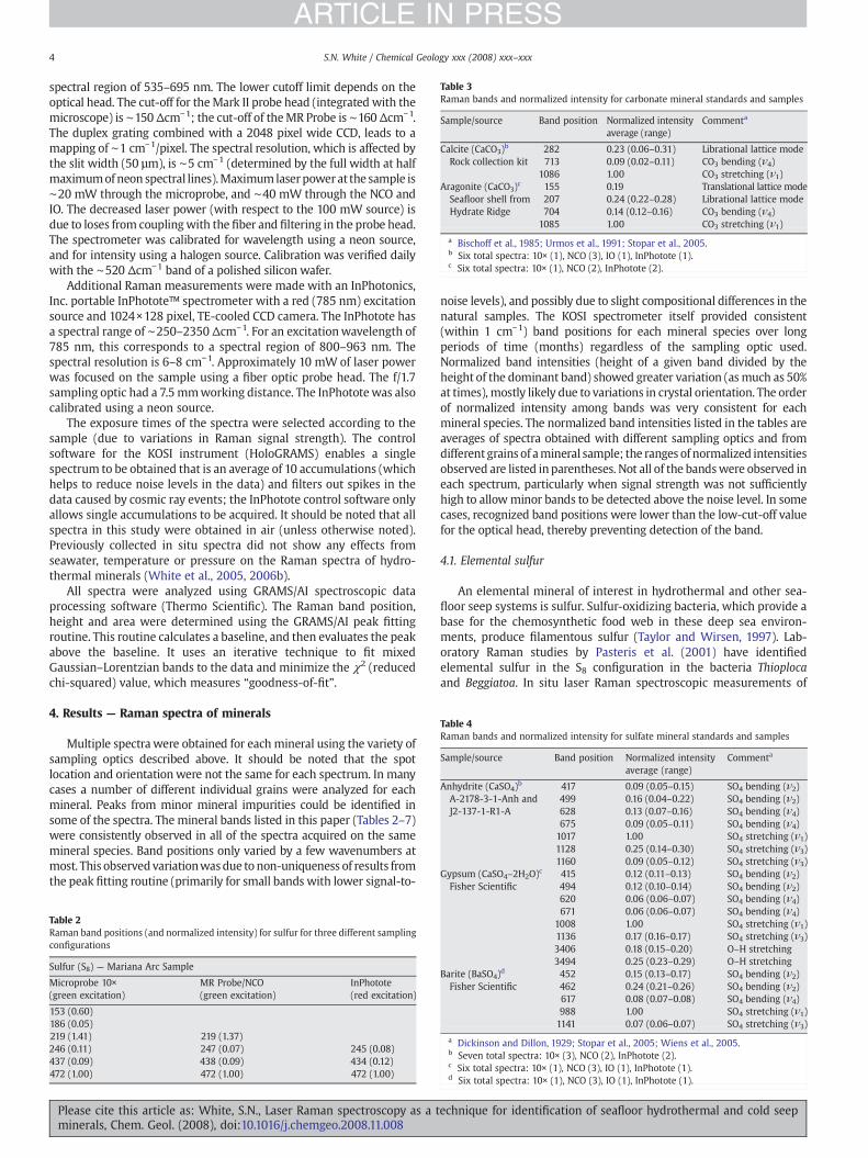
Table 3Raman bands and normalized intensity for carbonate mineral standards and samples

Sample/source Band position Normalized intensityaverage (range)

Commenta

Calcite (CaCO3)b 282 0.23 (0.06–0.31) Librational lattice modeRock collection kit 713 0.09 (0.02–0.11) CO3 bending (ν4)

1086 1.00 CO3 stretching (ν1)Aragonite (CaCO3)c 155 0.19 Translational lattice modeSeafloor shell fromHydrate Ridge

207 0.24 (0.22–0.28) Librational lattice mode704 0.14 (0.12–0.16) CO3 bending (ν4)

1085 1.00 CO3 stretching (ν1)

a Bischoff et al., 1985; Urmos et al., 1991; Stopar et al., 2005.b Six total spectra: 10× (1), NCO (3), IO (1), InPhotote (1).c Six total spectra: 10× (1), NCO (2), InPhotote (2).

Table 4Raman bands and normalized intensity for sulfate mineral standards and samples


Commenta

Anhydrite (CaSO4)b 417 0.09 (0.05–0.15) SO4 bending (ν2)A-2178-3-1-Anh andJ2-137-1-R1-A

499 0.16 (0.04–0.22) SO4 bending (ν2)628 0.13 (0.07–0.16) SO4 bending (ν4)675 0.09 (0.05–0.11) SO4 bending (ν4)1017 1.00 SO4 stretching (ν1)1128 0.25 (0.14–0.30) SO4 stretching (ν3)1160 0.09 (0.05–0.12) SO4 stretching (ν3)

Gypsum (CaSO4–2H2O)c 415 0.12 (0.11–0.13) SO4 bending (ν2)Fisher Scientific 494 0.12 (0.10–0.14) SO4 bending (ν2)


ARTICLE IN PRESS

spectral region of 535–695 nm. The lower cutoff limit depends on theoptical head. The cut-off for theMark II probe head (integrated with themicroscope) is ∼150 Δcm−1; the cut-off of theMR Probe is ∼160 Δcm−1.The duplex grating combined with a 2048 pixel wide CCD, leads to amapping of ∼1 cm−1/pixel. The spectral resolution, which is affected bythe slit width (50 µm), is ∼5 cm−1 (determined by the full width at halfmaximumofneon spectral lines).Maximumlaserpowerat the sample is∼20 mW through the microprobe, and ∼40 mW through the NCO andIO. The decreased laser power (with respect to the 100 mW source) isdue to loses from couplingwith the fiber and filtering in the probe head.The spectrometer was calibrated for wavelength using a neon source,and for intensity using a halogen source. Calibration was verified dailywith the ∼520 Δcm−1 band of a polished silicon wafer.

Additional Raman measurements were made with an InPhotonics,Inc. portable InPhotote™ spectrometer with a red (785 nm) excitationsource and 1024×128 pixel, TE-cooled CCD camera. The InPhotote hasa spectral range of ∼250–2350 Δcm−1. For an excitationwavelength of785 nm, this corresponds to a spectral region of 800–963 nm. Thespectral resolution is 6–8 cm−1. Approximately 10 mW of laser powerwas focused on the sample using a fiber optic probe head. The f/1.7sampling optic had a 7.5mmworking distance. The InPhototewas alsocalibrated using a neon source.

The exposure times of the spectra were selected according to thesample (due to variations in Raman signal strength). The controlsoftware for the KOSI instrument (HoloGRAMS) enables a singlespectrum to be obtained that is an average of 10 accumulations (whichhelps to reduce noise levels in the data) and filters out spikes in thedata caused by cosmic ray events; the InPhotote control software onlyallows single accumulations to be acquired. It should be noted that allspectra in this study were obtained in air (unless otherwise noted).Previously collected in situ spectra did not show any effects fromseawater, temperature or pressure on the Raman spectra of hydro-thermal minerals (White et al., 2005, 2006b).

All spectra were analyzed using GRAMS/AI spectroscopic dataprocessing software (Thermo Scientific). The Raman band position,height and area were determined using the GRAMS/AI peak fittingroutine. This routine calculates a baseline, and then evaluates the peakabove the baseline. It uses an iterative technique to fit mixedGaussian–Lorentzian bands to the data and minimize the χ2 (reducedchi-squared) value, which measures “goodness-of-fit”.

4. Results — Raman spectra of minerals

Multiple spectra were obtained for each mineral using the variety ofsampling optics described above. It should be noted that the spotlocation and orientationwere not the same for each spectrum. In manycases a number of different individual grains were analyzed for eachmineral. Peaks from minor mineral impurities could be identified insome of the spectra. The mineral bands listed in this paper (Tables 2–7)were consistently observed in all of the spectra acquired on the samemineral species. Band positions only varied by a few wavenumbers atmost. This observedvariationwasdue to non-uniqueness of results fromthe peak fitting routine (primarily for small bands with lower signal-to-

Table 2Raman band positions (and normalized intensity) for sulfur for three different samplingconfigurations

Sulfur (S8) — Mariana Arc Sample

Microprobe 10×(green excitation)

MR Probe/NCO(green excitation)

InPhotote(red excitation)

153 (0.60)186 (0.05)219 (1.41) 219 (1.37)246 (0.11) 247 (0.07) 245 (0.08)437 (0.09) 438 (0.09) 434 (0.12)472 (1.00) 472 (1.00) 472 (1.00)


noise levels), and possibly due to slight compositional differences in thenatural samples. The KOSI spectrometer itself provided consistent(within 1 cm−1) band positions for each mineral species over longperiods of time (months) regardless of the sampling optic used.Normalized band intensities (height of a given band divided by theheight of the dominant band) showed greater variation (asmuch as 50%at times), mostly likely due to variations in crystal orientation. The orderof normalized intensity among bands was very consistent for eachmineral species. The normalized band intensities listed in the tables areaverages of spectra obtained with different sampling optics and fromdifferent grains of amineral sample; the ranges of normalized intensitiesobserved are listed inparentheses. Not all of the bandswere observed ineach spectrum, particularly when signal strength was not sufficientlyhigh to allowminor bands to be detected above the noise level. In somecases, recognized band positions were lower than the low-cut-off valuefor the optical head, thereby preventing detection of the band.

4.1. Elemental sulfur

An elemental mineral of interest in hydrothermal and other sea-floor seep systems is sulfur. Sulfur-oxidizing bacteria, which provide abase for the chemosynthetic food web in these deep sea environ-ments, produce filamentous sulfur (Taylor and Wirsen, 1997). Lab-oratory Raman studies by Pasteris et al. (2001) have identifiedelemental sulfur in the S8 configuration in the bacteria Thioplocaand Beggiatoa. In situ laser Raman spectroscopic measurements of

620 0.06 (0.06–0.07) SO4 bending (ν4)671 0.06 (0.06–0.07) SO4 bending (ν4)

1008 1.00 SO4 stretching (ν1)1136 0.17 (0.16–0.17) SO4 stretching (ν3)3406 0.18 (0.15–0.20) O–H stretching3494 0.25 (0.23–0.29) O–H stretching

Barite (BaSO4)d 452 0.15 (0.13–0.17) SO4 bending (ν2)Fisher Scientific 462 0.24 (0.21–0.26) SO4 bending (ν2)

617 0.08 (0.07–0.08) SO4 bending (ν4)988 1.00 SO4 stretching (ν1)1141 0.07 (0.06–0.07) SO4 stretching (ν3)

a Dickinson and Dillon, 1929; Stopar et al., 2005; Wiens et al., 2005.b Seven total spectra: 10× (3), NCO (2), InPhotote (2).c Six total spectra: 10× (1), NCO (3), IO (1), InPhotote (1).d Six total spectra: 10× (1), NCO (3), IO (1), InPhotote (1).



Table 5Anhydrite Raman band positions (and normalized intensity) from two samples usingtwo different optics

A-2178-33-1-Anh (grain 2) J2-137-1-R1-A

10× NCO 10×a NCOb

417 (0.06) 417 (0.07) 418 (0.10) 417 (0.10)499 (0.20) 500 (0.19) 500 (0.17) 500 (0.15)628 (0.15) 628 (0.15) 628 (0.11) 628 (0.13)675 (0.08) 676 (0.09) 676 (0.05) 676 (0.10)1017 (1.00) 1017 (1.00) 1017 (1.00) 1017 (1.00)1128 (0.25) 1128 (0.28) 1128 (0.14) 1129 (0.29)1160 (0.12) 1160 (0.11) 1160 (0.09) 1160 (0.10)

a Black matrix.b Grey inclusion near gold area.

Table 7Chalcopyrite Raman band positions (and normalized intensity) from one sample usingthree different optics

A-2003-7-1a5 (Chalcopyrite)

10× NCO IO

265 (0.10) 266 (0.17) 267 (0.10)291 (1.00) 291 (1.00) 291 (1.00) 291 (1.00) 291 (1.00)320 (0.13) 320 (0.15) 322 (0.09) 320 (0.12) 320 (0.12)352 (0.09) 352 (0.09) 353 (0.11) 354 (0.10) 351 (0.10)456 (0.16) 458 (0.44)471 (0.66) 471 (1.36) 470 (1.1) 470 (0.81)


ARTICLE IN PRESS

bacterial mats at the Hydrate Ridge site have also detected the pres-ence of S8 sulfur (White et al., 2006b). Sulfur is also produced hy-drothermally and in volcanic eruptions (Nakamura et al., 2006). Themineral sample analyzed here is not biogenic but has the same S8configuration as biogenic sulfur.

S8 sulfur has an orthorhombic crystal structure and is a strongRaman scatterer. The dominant Raman bands of sulfur are at ∼219 and472Δcm−1. Additionalminor bands are at∼153, 437, 246 and 187Δcm−1

(Fig. 2). The bands in the 100–300 Δcm−1 region are due to S–S–Sbending and the bands in the 400–500 Δcm−1 region are due to S–Sstretching (Ozin,1969; Harvey and Butler,1986). The band positions andrelative intensities for sulfur obtained with the microprobe/10×, MRProbe/NCO, and InPhotote (red excitation) are listed in Table 2. Therelative intensities are listed with respect to the ∼472 Δcm−1 band,which is the dominant band present in all three spectra. The 219 Δcm−1

band has a higher intensity than the band chosen for normalization, butit is not recorded by the InPhotote instrument due to its light rejectionup to∼250Δcm−1. Pure sulfur has little fluorescence under either greenor red excitation. The spectral data obtained in this study correspond

Table 6Raman bands and normalized intensity for sulfide mineral standards and samples


Comment

Pyrite (FeS2)a 343 0.89 (0.72–0.98)A-2178-3-1-Py 379 1.00

430 0.08 (0.07–0.09)Marcasite (FeS2)b 323 1.00J2-135-5-R1-Mc 386 0.15 (0.08–0.26)

Chalcopyrite (CuFeS2)c 265 0.17 (0.10–0.25) Cu–S bandA-2003-7-1a5, J2-137-1-R1-A,and Wards Natural Science

291 1.00 Fe–S band320 0.21 (0.09–0.33) Fe–S band352 0.17 (0.08–0.24) Fe–S band456 0.22 (0.06–0.44)471 0.71 (0.09–1.36) Cu–S band

Isocubanite (CuFe2S3)d 351 0.70 (0.65–0.79)2467 RO1 P14MC 386 1.00

441 0.11 (0.10–0.11)Sphalerite ((Zn,Fe)S)e 298 1.00 Fe–S bandWards Natural Science 309 0.40 (0.33–0.43) Fe–S band

329 0.47 (0.42–0.52) Fe–S band340 0.13 (0.12–0.17) Fe–S band350 0.22 (0.07–0.38) Zn–S band

Wurtzite ((Zn,Fe)S)f 294 1.00 Fe–S band2944-3-s1-w1 308 0.38 (0.27–0.60) Fe–S band

326 0.83 (0.78–0.88) Fe–S band352 0.12 (0.09–0.17) Zn–S band1167 0.10 (0.09–0.10)

a Five total spectra: 10× (1), NCO (4).b Seven total spectra: 10× (3), NCO (4).c Ten total spectra: 10× (7), NCO (3).d Three total spectra: 10× (3).e Six total spectra: 10× (5), IO (1).f Five total spectra: 10× (2), NCO (3).


well to data reported in the literature for elemental sulfur analyzed inthe lab (Edwards et al., 1997) and filamentous sulfur produced bybacterialmats analyzed in the lab (Pasteris et al., 2001) and in situ on theseafloor (White et al., 2006b).

4.2. Carbonates

Calcite and aragonite are two of the polymorphs of calciumcarbonate (CaCO3), and both can be produced biologically. Calcite istrigonal, while aragonite has an orthorhombic crystal structure. Bivalveshells present at hydrothermal and cold seep sites are composed ofcalcium carbonate. Authigenic carbonate crusts are formed at cold seepsites and can contain calcite and high-Mg calcite. Laboratory Ramanstudies of individual shells have shown the presence of calcite and/oraragonite. In situ laser Raman spectroscopy measurements have alsoidentified calcite and aragonite in shells on the seafloor (White et al.,2005, 2006b).

As shown in spectra of the mineral standards and natural samplesanalyzed in this study, the dominant Raman band of both commoncrystal structures of calcium carbonate is at ∼1085 Δcm−1 due to thesymmetric stretching (ν1 vibration) of carbonate (CO3). A minor,lattice mode band is also present at ∼155 Δcm−1. Because calcite andaragonite have different lattice structures, the positions of some oftheir minor Raman bands are different. Calcite has minor bands at∼282 and 713 Δcm−1; aragonite has minor bands at ∼207 and704 Δcm−1 (Fig. 3). The bands below 300 Δcm−1 are lattice modes,while the bands near 700 Δcm−1 are due to the in-plane bending (ν4

vibration) of CO3 (Bischoff et al., 1985; Urmos et al., 1991; Stopar et al.,2005). A veryweak band at ∼1435Δcm−1 for calcite and ∼1462Δcm−1

for aragonite was sometimes observed in spectra of sufficient signalstrength; this is due to the anti-symmetric stretch (ν3 vibration). TheRaman band positions of both calcite and aragonite were veryconsistent regardless of the sampling optic or excitation wavelength.However, the normalized intensities (band height divided by theheight of the ∼1085 Δcm−1 band) showed some variation for calcite.This variation appeared to be somewhat related to the area beinganalyzed (i.e., whether the area was transparent or more opaque).Large, single, translucent crystals are more susceptible to opticalscattering effects caused by anisotropy within the crystal. In opaqueaggregates of fine grained crystals, the laser spot illuminates a largenumber of crystals in various orientations thus averaging outorientation effects. Spectra of aragonite were collected from boththe inside and outside of the shell sample. Raman band positions andnormalized intensities were very consistent for all of the aragonitespectra. Table 3 shows the band positions and the variations innormalized intensity for six spectra of each sample collected with thefollowing optics: calcite — 10× (1), NCO (3), IO (1), InPhotote (1);aragonite — 10× (1), NCO (3), InPhotote (2).

The spectrum of geological calcite collected with green excitationshows an inclined baseline due to some fluorescence of the sample(Fig. 3). However, the intensity of the fluorescence is not sufficient toobscure the Raman bands. The broad fluorescence observed fromcalcite in this study peaks at ∼2900 Δcm−1 (∼629 nm) (not shown).



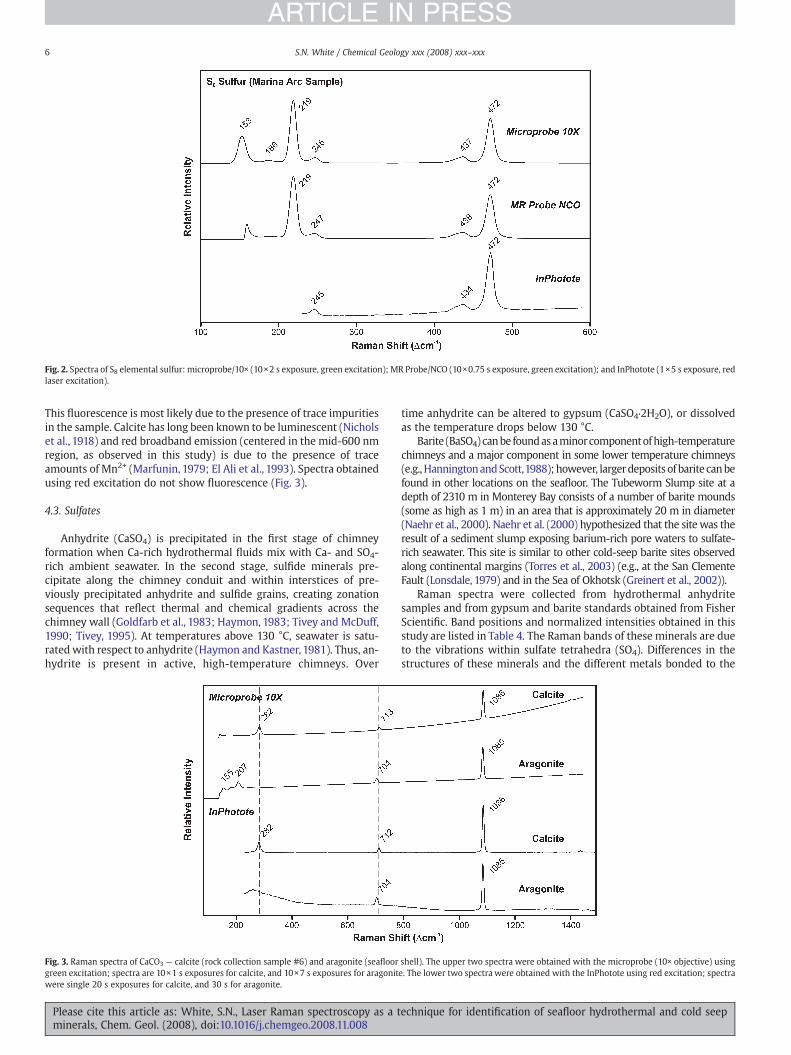
Fig. 2. Spectra of S8 elemental sulfur: microprobe/10× (10×2 s exposure, green excitation); MR Probe/NCO (10×0.75 s exposure, green excitation); and InPhotote (1×5 s exposure, redlaser excitation).


ARTICLE IN PRESS

This fluorescence is most likely due to the presence of trace impuritiesin the sample. Calcite has long been known to be luminescent (Nicholset al., 1918) and red broadband emission (centered in the mid-600 nmregion, as observed in this study) is due to the presence of traceamounts of Mn2+ (Marfunin, 1979; El Ali et al., 1993). Spectra obtainedusing red excitation do not show fluorescence (Fig. 3).

4.3. Sulfates

Anhydrite (CaSO4) is precipitated in the first stage of chimneyformation when Ca-rich hydrothermal fluids mix with Ca- and SO4-rich ambient seawater. In the second stage, sulfide minerals pre-cipitate along the chimney conduit and within interstices of pre-viously precipitated anhydrite and sulfide grains, creating zonationsequences that reflect thermal and chemical gradients across thechimney wall (Goldfarb et al., 1983; Haymon, 1983; Tivey and McDuff,1990; Tivey, 1995). At temperatures above 130 °C, seawater is satu-rated with respect to anhydrite (Haymon and Kastner, 1981). Thus, an-hydrite is present in active, high-temperature chimneys. Over

Fig. 3. Raman spectra of CaCO3 — calcite (rock collection sample #6) and aragonite (seafloorgreen excitation; spectra are 10×1 s exposures for calcite, and 10×7 s exposures for aragonitwere single 20 s exposures for calcite, and 30 s for aragonite.


time anhydrite can be altered to gypsum (CaSO4·2H2O), or dissolvedas the temperature drops below 130 °C.

Barite (BaSO4) canbe foundasaminorcomponentofhigh-temperaturechimneys and a major component in some lower temperature chimneys(e.g.,HanningtonandScott,1988);however, largerdeposits of barite canbefound in other locations on the seafloor. The Tubeworm Slump site at adepth of 2310 m in Monterey Bay consists of a number of barite mounds(some as high as 1 m) in an area that is approximately 20 m in diameter(Naehr et al., 2000). Naehr et al. (2000) hypothesized that the site was theresult of a sediment slump exposing barium-rich pore waters to sulfate-rich seawater. This site is similar to other cold-seep barite sites observedalong continental margins (Torres et al., 2003) (e.g., at the San ClementeFault (Lonsdale, 1979) and in the Sea of Okhotsk (Greinert et al., 2002)).

Raman spectra were collected from hydrothermal anhydritesamples and from gypsum and barite standards obtained from FisherScientific. Band positions and normalized intensities obtained in thisstudy are listed in Table 4. The Raman bands of these minerals are dueto the vibrations within sulfate tetrahedra (SO4). Differences in thestructures of these minerals and the different metals bonded to the

shell). The upper two spectra were obtained with the microprobe (10× objective) usinge. The lower two spectra were obtained with the InPhotote using red excitation; spectra




ARTICLE IN PRESS

sulfate ion (or the presence of H2O) cause slight differences in theposition of the Raman bands (Fig. 4a). The dominant Raman band isdue to the symmetric stretching (ν1 vibration) of SO4 and is located at∼1000 Δcm−1: ∼1017 Δcm−1 for anhydrite, ∼1008 Δcm−1 for gypsum,and ∼988 Δcm−1 for barite. The intensities of all bands werenormalized by dividing each peak height by the peak height for thisdominant band. The ν2 vibration (in-plane bending) generates bandsin the 400–500 Δcm−1 region, the ν4 vibration (out-of-plane bending)generates bands in the 600–700 Δcm−1 region, and the ν3 vibration(asymmetric stretching) generates bands in the 1100–1200 Δcm−1

region. Due to the incorporation of water molecules, gypsum also hasO–H stretching bands at ∼3406 and 3494 Δcm−1 (not shown) whichwere detected using the KOSI instrument under green excitation.

Anhydrite spectra were collected from relatively pure anhydritegrains (A2178-3-1-Anh) and from sample J2-137-1-r1-a, which is asample from a chimney wall (Fig. 5). Anhydrite is located throughoutsample J2-137-1-r1-a as visible inclusions (∼0.5 mm) and incorpo-rated in a black matrix of ZnS. Table 5 compares Raman band positionsand normalized band intensities for both of these samples obtainedwith the 10× and NCO sampling optics. The band positions and

Fig. 4. a. Raman spectra of sulfates obtained with the microprobe (10× objective) and green ebarite spectrum is 10×7 s. b. Raman spectra of sulfates obtained with the InPhotote and redgypsum.


normalized intensities are very consistent for both the non-mineralicanhydrite samples and anhydrite incorporated in a matrix of otherminerals. The data obtained in this study also correspond well tovalues found in the literature (e.g., Dickinson and Dillon, 1929; Stoparet al., 2005; Wiens et al., 2005).

No fluorescence is observed in the sulfate spectra using a greenexcitation laser (Fig. 4a) or in the gypsum or barite spectra using a redexcitation laser (Fig. 4b). However, the spectrum of anhydrite acquiredusing red excitation contains non-Raman bands in the 1200–1800 Δcm−1 region (only two of these bands are shown in Fig. 4b).These may be fluorescence bands due to impurities or trace materialsin the hydrothermal anhydrite. No significant impurity phases ordiscolorations were visible under the microscope, but the presence ofMn and rare earth elements has been shown to produce luminescentbands in natural anhydrite (Marfunin, 1979).

4.4. Sulfides

High-temperature black smoker chimneys are dominated by sul-fide phases, in addition to the previously mentioned anhydrite. The

xcitation. The anhydrite spectrum is 10×10 s; the gypsum spectrum is 10×20 s; and theexcitation. All spectra are single exposures of 10 s for anhydrite and barite, and 30 s for



Fig. 5. Hydrothermal chimney samples from an active open conduit smoker, Kilo Moana vent field, Eastern Lau Spreading Center (J2-137-1-R1-A) and from an inactive chimney from11N on the East Pacific Rise. (From WHOI seafloor sulfide collection, M.K. Tivey).


ARTICLE IN PRESS

major phases include chalcopyrite (CuFeS2), pyrite (FeS2), andpolymorphs sphalerite and wurtzite ((Zn,Fe)S)). Additional, minorsulfide phases include marcasite (FeS2), pyrrhotite (Fe(1 − x)S), andisocubanite (CuFe2S3) (e.g., Haymon and Kastner, 1981; Rona et al.,1986; Tivey and Delaney, 1986). Most of these sulfides are Ramanactive (Fig. 6). Pyrrhotite has variable composition, and two structuralforms— hexagonal andmonoclinic. A number of bands were observedin pyrrhotite spectra obtained in this study. However, based ontheoretical derivations (Mernagh and Trudu, 1993; Kroumova et al.,2003), none of the vibrational modes of either form of pyrrhotite areRaman active. Some of the bands observed appear to be due to sulfurand sulfate impurities; the remaining bands are likely the result ofnarrow band fluorescence and are highly variable.

The Raman bands of sulfide minerals identified in this study andtheir normalized intensities are listed in Table 6. The Raman signalstrength for sulfides was lower than that of the minerals previouslydiscussed. Due to the lower signal-to-noise and the fact that some ofthe bands overlap one another, the Raman band positions sometimesvaried up to a few wavenumbers in analyses of different samples ofthe same mineral. However, this did not prohibit proper mineral

Fig. 6. Raman spectra of sulfides obtained with the microprobe (10× objective) usinggreen excitation. The pyrite, marcasite, chalcopyrite andwurtzite spectra are all 10×60 sexposures; marcasite is 10×15 s.


identification. Mernagh and Trudu (1993) investigated a number ofprimarily terrestrial sulfides using a 514 nm Ar ion laser as theexcitation source. The data in this work corresponds well to Mernaghand Trudu (1993) and other previous work on terrestrial samples (e.g.,Ushioda, 1972; Turcotte et al., 1993; Pasteris, 1998; Wang et al., 2004).

Pyrite and marcasite are polymorphs of FeS2 (Fig. 6); pyrite has acubic symmetry while marcasite is orthorhombic. Pyrite has twodominant Raman bands at ∼343 and 379 Δcm−1, and a minor band at∼430 Δcm−1 (Table 5). These bands correspond to the Ag, Eg, and Tg(3)vibrational modes, respectively. By deconvolving the dominantobserved peaks, two minor bands are also observed at ∼350 and377 Δcm−1 (the Tg(1) and Tg(2) vibrational modes) (Ushioda, 1972;Blanchard et al., 2005). Spectra obtained onmarcasite (particularly withthemicroprobe) often showed additional mineral species such as bariteand anhydrite, which presumably were intergrown on a fine scale. Thedominant bands that appear to be those of marcasite are ∼323 and386 Δcm−1 (Table 6). These bands correspond to those identified in theliterature,whichhave been assigned to theAg stretchingmode (Lutz andMüller, 1991; Mernagh and Trudu, 1993). An additional band at∼394 Δcm−1 was observed in many of the spectra as a minor shoulderof the 386Δcm−1 band. Lutz andMüller (1991) also observe this band insome spectra and associate it with the B1g librational mode. The Ramanspectra of pyrite and marcasite obtained with the red excitation laserweremuchweaker in intensity than thoseobtainedwith the green laser,but the dominant bands (∼343 and 379Δcm−1 for pyrite, and ∼323 and386 Δcm−1 for marcasite) were observed.

Chalcopyrite (CuFeS2) has a tetragonal crystal structure. There arefew data in the literature on the Raman spectrum of chalcopyrite.Spectra obtained on chalcopyrite in this work were occasionallycontaminated by the presence of sulfates such as barite. Unlike otherminerals in this study, chalcopyrite spectra were collected from bothhomogeneous samples obtained fromWard's Natural Sciences and twochimney wall samples (Fig. 5) that clearly show the zonation from achalcopyrite-rich “inner” conduit wall outward to a Zn–S matrix. Traceamounts of sulfates are also present throughout the chimney samples.Due to the strong Raman scattering of sulfates, a minor amount of asulfate in the beam path can create significant peaks in the spectrum.The characteristic peaks of chalcopyrite include a dominant band at∼291 and minor bands at ∼265, 320, and 352 Δcm−1 (Table 6, Fig. 6).These bands correspond to those observed by Mernagh and Trudu(1993). A large band at ∼471 Δcm−1 was often observed in the spectrafrom the chimney samples which varied in intensity with respect to theother Raman bands. While it is similar in position to the strong sulfurband (∼474Δcm−1), the lack of the 219Δcm−1 sulfur band suggests thatthe 471 band is not due to the presence of trace amounts of sulfur. TheUniversity of Arizona's online RRUFF database (Downs, 2006) containsspectra from four samples of chalcopyrite. The ∼471 Δcm−1 band is




ARTICLE IN PRESS

present in some of these spectra, but not others. In this study, theintensity of the 471 band is higher for the A2003-7-1a5 sample than forthe J2-137-1-r1-a sample (0.92 averaged normalized intensity forsample A2003-7-1a5 compared to 0.14 for sample J2-137-1-r1-a). The265 and 471 Δcm−1 bands are Cu–S bands (Smith and Clark, 2002;Branch et al., 2003). Thus, the higher intensity observed in one samplemaybedue to thepresence of Cu–S tarnishespresenton the sample. Thisis discussed in more detail in the next section. Table 7 lists the bandpositions and normalized intensity for spectra of sample A2003-7-1a5collected using the 10× objective, NCO, and IO sampling optics (all usinggreen excitation). Not all of the bands were observed in each case. Asstated above, the 471Δcm−1 band shows great variability in normalizedintensity.

Sphalerite and wurtzite ((Zn,Fe)S) are polymorphs of zinc sulfidewhose crystal structures accommodate a number of replacements forzinc, including iron. Sphalerite has a cubic crystal structure, andwurtzite is hexagonal. The sphalerite sample has Raman bands at∼298 (dominant), 309, 329, 340, and 350 Δcm−1 (Table 6, Fig. 6). The∼350 band is a Zn–S band, whereas the lower wavenumber bands areFe–S bands. The normalized band intensities observed in this studycorrespond to those for low-Fe sphalerite (∼7 wt.% Fe, ∼57 wt.% Zn inKharbish (2007)). Wurtzite has similar band positions at ∼294, 308,326, and 352 Δcm−1 (Table 6, Fig. 6), which correspond to data inMernagh and Trudu (1993). Within the individual sphalerite andwurtzite spectra, the Raman bands are quite close together, such thatsome of the minor bands are not resolved in the raw spectra. Theindividual bands can be identified by deconvolving the spectra with apeak-fitting program (such as GRAMS/AI).

Isocubanite (CuFe2S3) is a cubic structured polymorph of cubanite(previously referred to as iss-cubanite) (Caye et al., 1988). Samples ofisocubanite (identified by petrographic microscope under reflectedlight) were analyzed in thin section using the Raman microprobe (10×objective). The use of micro-Raman spectroscopy to analyze mineralsin thin sectionwas described byMao et al. (1987). Two primary Ramanbands are observed at ∼351 and 386 Δcm−1 (Table 6, Fig. 7). A minor,broader band is also observed at ∼441 Δcm−1. This sample was notanalyzed with the NCO or IO remote optics, or with red excitation.

Raman spectra of the other sulfides were also obtained with redexcitation. However, while all of the characteristic peaks were ob-served, the signal strengths were significantly lower (and thus noisier)than with green excitation. Peak fits for these data were not includedin Table 6 due to the low signal quality.

5. Application — Raman spectra of recovered hydrothermalchimney samples

The data obtained in this study were applied to the analysis of twochimney wall samples. The NCO sampling optic (with green excitation)was used to collect Raman spectra in a profile across visible zonationpatterns of each sample to identify the mineral species present.

Fig. 7. Raman spectrum of isocubanite obtained from a thin section using the microp


5.1. Sample J2-137-1-r1-a

This sample is a portion of a chimney wall recovered from the KiloMoana vent field on the Eastern Lau Spreading Center (Tivey et al.,2005). The “inner”wall is dominated by a gold-colored mineral, whilethe “outer” section is dominantly black in color. A series of sevenspectra was collected with the MR Probe/NCO across the sawn sampleface shown in Fig. 5. Five representative spectra from this scan areshown in Fig. 8. The spectrum from the outer-most portion (furthestfrom the gold) contains Raman bands indicating the presence ofwurtzite (∼296, 308 and 330 Δcm−1) and pyrite (∼346 and 378 Δcm−1)(Fig. 8a). Moving towards the gold region the spectra are dominated bysphaleritewith somepyrite and/or anhydrite (Fig. 8b,c). A spectrumwascollected from awhite inclusion in the gold region, whichwas primarilyanhydrite (Fig. 8d). Moving into the gold region toward the “inner” rimof the sample, the spectra are dominated by chalcopyrite (∼291, 320,352 Δcm−1) (Fig. 8e).

The Raman spectra agree reasonably well with visual observationsfrom a thin section taken from the same chimney: the chimneyconduit is lined with cubanite or chalcopyrite, grading out tointermediate solid solution (intergrowths of cubanite and chalcopyritelamellae) with minor inclusions of pyrite; there is then an abrupttransition to amixture of wurtzitewithminor chalcopyrite, pyrite, andanhydrite, with outermost portions a mixture of sphalerite and/orwurtzite, pyrite, and amorphous silica with minor anhydrite present.

Sulfate bandswere observed inmanyof the spectra near∼990Δcm−1

(with attendant minor bands in the 400 and 600 Δcm–1 regions).However, no visible grains of sulfate minerals (other than anhydrite)were observed in this sample under the microprobe using reflectedlight or in the thin section from the same chimney viewed with apetrographic microscope. Given that this sample was recovered andremoved from seawater and dried without any prior rinsing, it ispossible that the sulfate bands observed are due to fine-grainedsulfate salts precipitated from seawater on the surface and ininterstitial spaces. Sulfates such as CuSO4, FeSO4, MgSO4, MnSO4,KSO4, NaSO4, and ZnSO4 all have primary Raman bands in the ∼975 to1025 Δcm−1 region. To test the above hypothesis, a piece of the samechimneywall was soaked in distilledwater and then rinsed and dried.A white precipitate was present on most surfaces after drying, andRaman analyses of these areas produced sulfate bands, though atslightly different band positions. This is consistent with differentsulfate salts having reprecipitated during drying. The sample wasthen placed in deionized water. Raman analyses of the submergedsample were performed (using the microprobe with 10× objective),and clear sulfide bands were observed at ∼299, 330 and 351 Δcm−1.The only “extra” band observed in the ∼400 to 1200 Δcm−1 regionwas at 981 Δcm−1, which is the location of the dissolved sulfate ionband. These analyses support the initial hypothesis that the bands inthe original sample do indeed represent precipitated salts frominterstitial seawater.

robe (10× objective) and green excitation. The spectrum is a 10×30 s exposure.



Fig. 8. Scan of spectra across the sample J2-137-1-r1-a (Fig. 5) using the NCO and green excitation. Spectra (a), (b) and (c) are from the black-colored region of the sample; spectrum(d) is from a white inclusion, spectrum (e) is from the gold-colored region. Mineral peaks are identified as wurtzite (Wtz), pyrite (Pyr), sphalerite (Sph), anhydrite (Anh) andchalcopyrite (Chalc). All spectra are 10×15 s exposures.


ARTICLE IN PRESS

Sulfate minerals are strong Raman scatters compared to sulfides.Therefore, even a small amount of precipitated sulfate can produce avisible Raman band during long exposures. This is not an issue for insitu analyses. However, if recovered samples are analyzed using laserRaman spectroscopy, the likely presence of dried salts needs to beconsidered when interpreting data.

5.2. Sample A2003-7-1a5

Sample A2003-7-1a5 is from an inactive sealed chimney recoveredfrom11°Non theEast PacificRise in1988.Bandsof tarnishareobservedonone side of the sample (Fig. 5). These tarnishes vary in color from black tobluish-green to purple, and are assumed to be a progression from bornite(Cu5FeS4) to covellite (CuS) to chalcocite (Cu2S) todigenite (Cu9S5)— losingFe and gaining Cu (Tivey, pers. comm.). Spectra were obtained from anuntarnished region of the sample and from the blackish, bluish-green, andpurplish regions of the tarnish (Fig. 9). The spectrum from theuntarnished

Fig. 9. Scan of spectra across the tarnishes on sample A2003-7-1a5 (Fig. 5) using the NCO andsample away from the tarnishes. All spectra are 10×15 s exposures.


region was clearly chalcopyrite with band positions (and normalizedintensities) of: ∼291 (1.00), 320 (0.21), 354 (0.26) and 470 (0.91) Δcm−1.Moving from the purplish tarnish to the blackish tarnish, Cu–S bands at∼265 and 472 Δcm−1 increase in intensity, while the Fe–S bands at ∼291,320, and 354 Δcm−1 decrease in intensity. The Raman spectrum ofcovellite (Cu–S) is characterized by a dominant band at∼472Δcm−1 and aminor band at ∼264 Δcm−1 (Mernagh and Trudu, 1993; Smith and Clark,2002). Mernagh and Trudu (1993) were unsuccessful in obtaining Ramanspectra from bornite, chalcocite and digenite. The covellite band positionscorrespond to the Cu–S bands of chalcopyrite (Table 6). It is not clearwhether the Fe–Sbandsobserved in thepurplish andbluish-green tarnishspectra are due to thepresenceof Fe in the tarnish (e.g., bornite tarnish), orif they are due to the underlying chalcopyrite. Two pyrite bands (344 and378 Δcm−1) are also visible in the spectrum from the purplish tarnish(underlined in Fig. 9). The Raman spectrum of the blackish tarnish (whichmay bemore successful in covering the underlying chalcopyrite) suggeststhat it is a pure CuS mineral (i.e., covellite, chalcocite, or digenite).

green excitation. The chalcopyrite spectrum (bottom) was collected from an area on the




ARTICLE IN PRESS

6. Discussion

The data in this paper show that laser Raman spectroscopy is apowerful tool capable of identifying hydrothermal vent and cold seepminerals and distinguishing them from one another. The techniquecan be applied in the lab on whole samples, or thin sections, which isuseful for fine-grained intergrowths and inclusions or for in situanalysis (e.g., White et al., 2006b). The data obtained in this study(characteristic band positions and normalized intensities) can be usedwith a computer algorithm such as RaSEA (Breier et al., submitted forpublication) for automated mineral identification.

6.1. Relative Raman signal strength

The intensity of the Raman signal is a function of laser power, laserwavelength, and the Raman scattering efficiency of the sample. Sulfuris a strong Raman scatterer with a Raman scattering intensity an orderof magnitude greater than that of the carbonates and sulfates. Thesulfides produced the weakest Raman signal — three orders of mag-nitude lower than sulfur. This variation in Raman signal strengthexplains why small amounts of sulfur or sulfate minerals can produceobservable peaks in a sulfide sample (e.g., Fig. 8). Additionally, moretransparent minerals (such as anhydrite) may allow greater laser pen-etration and greater scattering within the sample than more opaqueminerals (such as pyrite). In the former, the scattering volume isgreater, resulting in a greater Raman signal.

6.2. Excitation wavelength

When recorded as the Raman shift, the band position in a Ramanspectrum is not dependent on excitation wavelength. Typical excita-tion wavelengths include 514 nm (Ar ion laser), 532 nm (frequencydoubled, Nd:YAG laser), 633 nm (He Ne laser), 785 nm (diode laser)and 1064 nm (Nd:YAG laser). However, Raman scattering intensity isinversely proportional to λ4, so 532 nm produces a stronger Ramansignal than 785 or 1064 nm. Green lasers (532 nm) are ideal for oceanwork because this wavelength corresponds to the transmission peakof water. The previously mentioned DORISS instrument (Brewer et al.,2004; Pasteris et al., 2004) and aircraft-based Raman instruments(Leonard et al., 1979; Becucci et al., 1999) used 532 nm lasers. For anin-water working distance of 1 cm, 99.95% of 532 nm laser power willbe transmitted compared to 97% of 785 nm laser power. However, for a15 cm working distance, 99.25% of 532 nm laser power will betransmitted while only 64% of 785 nm laser power will be transmitted.The backscattered radiation will also be attenuated by a similaramount.

The disadvantage of an excitation source in the blue–green is thatfluorescence can be generated by trace metals in minerals and bysome organic materials. For example, fluorometers designed to mea-sure chlorophyll a excite in the blue region (∼440–470 nm) and detectfluorescence in the red (∼685 nm). Methods for overcoming fluo-rescence are discussed by Ferraro et al. (2003) and include: changingthe excitation wavelength (into the red); using pulsed lasers todiscriminate the signals by time (Raman scattering is faster in re-sponse and shorter-lived than fluorescence (Matousek et al., 1999,2001)); and exposing the sample to prolonged laser irradiation tobleach out fluorescent impurities.

Spectra obtained from natural samples as a part of this studydemonstrate that hydrothermal minerals such as carbonates, sul-fates, and sulfides do not suffer from significant fluorescence whenanalyzed with green excitation. Use of red excitation also producedspectra with distinct Raman peaks. However, in the case of anhydrite,red excitation resulted in additional peaks most likely due to fluo-rescence from minor impurities. The use of red excitation also re-sulted in lower signal strengths (after accounting for differences inlaser power).


6.3. Sampling optics

Most of the samples were analyzed using three different samplingoptics: 1) the microprobe with the 10× objective, 2) the MR remoteprobe head with the non-contact optic (NCO), and 3) the MR remoteprobe head with the immersion optic (IO). MBARI's DORISS instru-ment is capable of using both an NCO behind a dome window and anIO (Brewer et al., 2004). The optics with shorter working distances(10× and IO; 5.8 and 3 mm, respectively) have a shorter depth of focus,smaller laser spot size, and a higher power density at the sample. TheNCO has a longer working distance (6.4 cm), a longer depth of focus,and a lower power density. Note that all of this workwas done in air. Inwater, the working distance and depth of focus will be slightly greater.However, even in water, the depth of focus is small enough that somemechanism of focusing or positioning the laser spot (White et al.,2005) is needed.

It is difficult to compare the efficiencies of the optics because thesignal intensity is affected by a number of factors. The most obviousfactors are laser power and exposure time. The datawere normalized bydividing the spectra by exposure time and laser power to account forthese variations. Another factor to consider when selecting a samplingoptic is proper positioning. For opaque samples, the focal point of thelasermust be positioned at the surface of the sample. The depth of focusfor the optics used here range from millimeter to sub-millimeter. Themicroscope objective could be focused visually by sighting through theobjective via a camera. The remote head optics, however, do not havethrough-the-lens visualization capabilities and were focused by adjust-ing the position of the sample to maximize peak heights in the spectra.For solid samples, crystal orientation can also have an impact on thesignal strength and depth of penetration into the sample. Thesevariations cannot be accounted for quantitatively.

Spectra were compared by looking at normalized peak height(divided by exposure time and laser power) of the dominant band andrelative order of peak intensities for the minor bands. In general, thenormalized peak heights of spectra obtained from the three opticswere around the same order of magnitude. The IO consistentlyprovided greater intensities than the NCO. This enhanced signal isexpected due to the higher power density it provides. The IO and 10×objective also have a slightly larger numerical aperture than the NCO(.25 vs. .17). The relative order of peak intensities of the minor bandswas also consistent for all of the sampling optics used.

7. Conclusion

Laser Raman spectroscopy is a powerful tool for identifying min-eral species in situ in the deep ocean. It is capable of obtaining highquality spectra of hydrothermally- and cold seep-relevant mineralssuch a carbonates, sulfates, and sulfides down to grain sizes below50 µm. In order to build a sea-going instrument optimized for mineralanalyses at these types of seafloor sites, detailed laboratory workmustbe performed to evaluate how readily the minerals of interest can bedistinguished spectroscopically and to understand how the spectraare affected by natural variation in mineral chemistry and differencesin instrument parameters.

High quality Raman spectra were obtained from standards andnaturally occurring mineral samples using both red and greenexcitation. Although organic compounds and impurities have thepotential to produce fluorescence (particularly with blue–greenexcitation), which can overwhelm the Raman signal, fluorescencewas not observed to be a significant problem for any of the samplesanalyzed here. The highest quality spectra (highest signal-to-noise)were obtained using green excitation (532 nm Nd:YAG laser) and asampling optic with a short depth of focus (and thus high powerdensity). Sulfur was the strongest Raman scatterer, followed by thecarbonates and sulfates. The sulfideminerals were theweakest Ramanscatters, but good quality spectra were obtained from these minerals




ARTICLE IN PRESS

as well. Characteristic Raman bands (and their relative intensities)were identified for each mineral (Tables 2–7), which correlated wellwith and built upon data found in the literature.

Based on the data from this work, a Raman system optimized forhydrothermal and cold seep minerals should have a spectral range of100–1800 Δcm−1. All of the characteristic Raman bands of the mineralsanalyzed fall within this range, as does the 1640 Δcm−1 water bendingband (against which Raman-active dissolved species can be normal-ized). The selection of a small spectral range also allows for higherspectral resolution. Because many of the sulfide minerals have Ramanbands that are very close in wavenumber, an instrument resolution of≤3 cm−1 would be preferable. 532 nm is the preferred excitationwavelength for theminerals analyzed in thiswork (particularly sulfates),because it produces a strong Raman signal and does not generatesignificantfluorescence. If organicmaterials (e.g., sediments) are presenton the surface of the sample of interest, some type of brushing orscraping may be required to clean the surface before Raman spectra areobtained. Green excitation also allows greater in-water stand-offdistanceswithout significant attenuation of the signal. Use of a samplingoptic with a 10 cm working distance (focal length) will decrease thepossibility of accidentally touching the optic to the side of a chimney,which can be∼350 °C. A longer focal length optic will also have a longerdepth of focus,whichmakes positioningof the focal point on the surfaceof the target easier. However, if work is to be done in areas of highsediment deposition or on hydrothermal plume particles that haveorganics present, then a 785 nm excitation laser with a ∼1 cmworkingdistance is preferable.

Operational challenges include positioning of the optical head,visualization of the area analyzed, and automation. Due to the smalldepth of focus of all of the sampling optics described, some form ofpositioner will be required to locate the laser spot on the target ofinterest. The three-degree-of-freedom Precision Underwater Positioner(White et al., 2005) developed for the DORISS instrument is an exampleof the type of system needed. For long-term Raman deployments athydrothermal vents, positioning will be a challenge, as vent deposittopography can change rapidly over time. User control through an ROVor seafloor cable is simplest, but at some time a mechanism forautomated positioning may be required. Regardless of how the opticalhead is positioned, visualization of the site – both on the scale of anindividual chimneyandon the scale of themeasurementbeingmade– isrequired to provide context for the spectra obtained.

The ability of laser Raman spectroscopy to optically identify min-eralogy in situ makes it an ideal instrument for extreme environmentssuch as other planets and the deep ocean. Planetary and oceanic ex-plorations require similar characteristics such as small size, low power,robustness, etc. Wang et al. (1998, 2003) have developed a small-scaleprototype for a Mars mission. The DORISS instrument (Brewer et al.,2004) is the first step in using Raman spectroscopy in the deep ocean.The development of new, smaller, smarter Raman instruments willgreatly improve our understanding of mineralogic and geochemicalprocesses occurring in these remote locations.

Acknowledgements

The author appreciates the assistance of Meg Tivey in procuring andidentifying hydrothermal mineral samples and for editorial commentson this manuscript. Job Bello and Kevin Spencer of EIC Labs, and RobForney of InPhotonics provided assistance in obtaining Raman spectrawith the InPhotote system. Post-doc John Breier and WHOI SummerStudent Fellow Abitha Murugeshu assisted with data collection. Thiswork was funded by the Cecil H. and Ida M. Green Technology Inno-vation Fund. Additional support was provided by the James S. Coles andCecily C. Selby Endowed Fund in Support of Scientific Staff and thePenzance Endowed Fund in Support of Assistant Scientists. This paperhas benefited from the comments of Jill Pasteris and an anonymousreviewer.


References

Aloisi, G., et al., 2000. Methane-related authigenic carbonates of eastern MediterraneanSea mud volcanoes and their possible relation to gas hydrate destabilisation. EarthPlanet. Sci. Lett. 184, 321–338.

Aloisi, G., et al., 2002. CH4-consuming microorganisms and the formation of carbonatecrusts at cold seeps. Earth Planet. Sci. Lett. 203, 195–203.

Alt, J.C., 1995. Subseafloor processes in mid-ocean ridge hydrothermal systems. In:Humphris, S.E., Zierenberg, R.A., Mullineaux, L.S., Thomson, R.E. (Eds.), SeafloorHydrothermal Systems: Physical, Chemical, Biological, and Geological Interactions.AGU, Washington, DC.

Baker, E.T., German, C.R., 2004. On the global distribution of hydrothermal vent fields.In: German, C.R., Lin, J., Parson, L.M. (Eds.), Mid-ocean Ridges: HydrothermalInteractions Between the Lithosphere and Oceans. AGU, Washington, DC.

Becucci, M., Cavalieri, S., Eramo, R., Fini, L., Materazzi, M., 1999. Accuracy of remotesensing of water temperature by Raman spectroscopy. Appl. Opt. 38 (6), 928–931.

Bischoff, W.D., Sharma, S.K., Mackenzie, F.T., 1985. Carbonate ion disorder in synthe-tic and biogenic magnesian calcites: a Raman spectral study. Am. Mineral. 70,581–589.

Blanchard, M., et al., 2005. Electronic structure study of the high-pressure vibrationalspectrum of sFeS2 Pyrite. J. Phys. Chem. B 109, 22,067–22,073.

Branch, M.S., Berndt, P.R., Botha, J.R., Leitch, A.W.R., Weber, J., 2003. Structure andmorphology of CuGaS2 thin films. Thin Solid Films 431–432, 94–98.

Breier, J.A., German, C.R., White, S.N., submitted for publication. Quantitative MineralSpeciation of Deep-SeaHydrothermal Particulates by Raman Spectroscopy and ExpertAlgorithm (RaSEA) Point Counting: Towards Autonomous In Situ Exploration and Ex-perimentation. Geochem. Geophys. Geosyst.

Brewer, P.G., et al., 2004. Development of a laser Raman spectrometer for deep-oceanscience. Deep-Sea Res. I 51. doi:10.1016/j.dsr.2003.11.005.

Caye, R., et al., 1988. Isocubanite, a new definition of the cubic polymorph of cubaniteCuFe2S3. Mineral. Mag. 52, 509–514.

Daly, K.L., et al., 2004. Chemical and biological sensors for time-series research: currentstatus and new directions. MTS J. 38 (2), 121–143.

Dickinson, R.G., Dillon, R.T., 1929. The Raman spectrum of gypsum. Proc. Natl. Acad. Sci.15 (9), 695–699.

Downs, R.T., 2006. The RRUFF Project: an integrated study of the chemistry, crystal-lography. Raman, and Infrared Spectroscopy of Minerals, 19th General Meeting ofthe International Mineralogical Association, Kobe, Japan, pp. O03–O13.

Edwards, H.G.M., Farwell, D.W., Turner, J.M.C., Williams, A.C., 1997. Novel environmentalcontrol chamber for FT-Raman spectroscopy: study of in situ phase change of sulfur.Appl. Spectrosc. 51 (1), 101–107.

El Ali, A., et al., 1993. Mn2+-activated luminescence in dolomite, calcite and magnesite:quantitative determination of manganese and site distribution by EPR and CL spec-troscopy. Chem. Geol. 104, 189–202.

Ferraro, J.R., Nakamoto, K., Brown, C.W., 2003. Introductory Raman Spectroscopy.Academic Press, San Diego, CA.

Goldfarb, M.S., Converse, D.R., Holland, H.D., Edmond, J.M., 1983. The genesis of hotspring deposits on the East Pacific Rise, 21°N. In: Ohmoto, H., Skinner, B.J. (Eds.),Economic Geology Monograph, pp. 184–197.

Greinert, J., Bollwerk, S.M., Derkachev, A., Bohrmann, G., Suess, E., 2002. Massive baritedeposits and carbonate mineralization in the Derugin Basin, Sea of Okhotsk:precipitation processes at cold seep sites. Earth Planet. Sci. Lett. 203, 165–180.

Hannington, M.D., Scott, S.D., 1988. Mineralogy and geochemistry of a hydrothermalsilica–sulfide–sulfate spire in the caldera of Axial Seamount, Juan de Fuca. Can.Mineral. 26 (3), 603–625.

Hannington, M.D., de Ronde, C.E., Petersen, S., 2005. Sea-floor tectonics and submarinehydrothermal systems. In: Hedenquist, J.W., Thompson, J.F.H., Goldfarb, R.J.,Richards, J.P. (Eds.), Economic Geology 100th Anniversary Volume. Society ofEconomic Geologists, Littleton, Colorado, pp. 111–141.

Harvey, P.D., Butler, I.S., 1986. Raman spectra of orthorhombic sulfur at 40 K. J. RamanSpectrosc. 17, 329–334.

Haskin, L.A., et al., 1997. Raman spectroscopy for mineral identification and quantificationfor in situ planetary surface analysis: a point count method. J. Geophys. Res. 102 (E8),19,293–19,306.

Haymon, R.M., 1983. Growth history of hydrothermal black smoker chimneys. Nature301, 694–698.

Haymon, R.M., Kastner, M., 1981. Hot spring deposits on the East Pacific Rise at 21°N:preliminary description of mineralogy and genesis. Earth Planet. Sci. Lett. 53,363–381.

Hessler, R.R., Kaharl, V.A., 1995. The deep-sea hydrothermal vent community. In:Humphris, S.E., Zierenberg, R.A., Mullineaux, L.S., Thomson, R.E. (Eds.), SeafloorHydrothermal Systems: Physical, Chemical, Biological, and Geological Interactions.AGU, Washington, DC.

Hester, K.C., et al., 2007. Gas hydrate measurements at Hydrate Ridge using Ramanspectroscopy. Geochim. Cosmochim. Acta 71, 2947–2959.

Hester, K.C., White, S.N., Peltzer, E.T., Brewer, P.G., Sloan, E.D., 2006. Raman spectroscopicmeasurements of synthetic gas hydrates in the ocean. Mar. Chem. 98, 304–314.

Kharbish, S., 2007. A Raman spectroscopic investigation of Fe-rich sphalerite: effect ofFe-substitution. Phys. Chem. Miner. 34, 551–558.

Kroumova, E., et al., 2003. Bilbao crystallographic server: useful databases and tools forphase-transition studies. Phase Transit. Multinatl. J. 76, 155–170.

Landsberg, G., Mandelstam, L., 1928. Eine neue Erscheinung bei der Lichtzerstreuung inKrystallen. Naturwissenschaften 16, 557–558.

Leonard, D.A., Caputo, B., Hoge, F.E., 1979. Remote sensing of subsurface water tem-perature by Raman scattering. Appl. Opt. 18 (11), 1732–1745.

Lonsdale, P.,1979. Adeep-seahydrothermal site ona strike–slip fault. Nature 281, 531–534.


http://dx.doi.org/10.1016/j.dsr.2003.11.005



ARTICLE IN PRESS

Luff, R., Wallmann, K., Aloisi, G., 2004. Numerical modeling of carbonate crust formationat cold vent sites: significance for fluid and methane budgets and chemosyntheticbiological communities. Earth Planet. Sci. Lett. 221, 337–353.

Lutz, H.D., Müller, B., 1991. Lattice vibration spectra. LXVIII. Single-crystal Raman spectraof marcasite-type iron chalcogenides and pnictides, FeX2 (X=S, Se, Te; P, As, Sb).Phys. Chem. Miner. 18, 265–268.

Mao, H., Hemley, R.J., Chao, E.C.T., 1987. The application of micro-Raman spectroscopy toanalysis and identification ofminerals in thin section. ScanningMicrosc.1 (2), 495–501.

Marfunin, A.S., 1979. Spectroscopy, Luminescence and Radiation Centers in Minerals.Springer-Verlag, Berlin. 352 pp.

Matousek, P., Towrie, M., Stanley, A., Parker, A.W., 1999. Efficient rejection of fluo-rescence from Raman spectra using picosecond Kerr gating. Appl. Spectrosc. 53 (12),1485–1489.

Matousek, P., et al., 2001. Fluorescence suppression in resonance Raman spectroscopyusing a high-performance picosecond Kerr gate. J. Raman Spectrosc. 32, 983–988.

Mernagh, T.P., Trudu, A.G., 1993. A laser Raman microprobe study of some geologicallyimportant sulphide minerals. Chem. Geol. 103, 113–127.

Naehr, T.H., Stakes, D.S., Moores, W.S., 2000. Mass wasting, ephemeral fluid flow, andbarite deposition on the California continental margin. Geology 28 (4), 315–318.

Nakamoto, K., 1997. Infrared and Raman Spectra of Inorganic and Coordination Com-pounds: Part A. John Wiley & Sons, Inc., New York, NY. 387 pp.

Nakamura, K., et al., 2006. Liquid and emulsified sulfur in submarine solfatara fields oftwo Northern Mariana arc volcanoes. Fall Meet. Suppls., Abstract V23B–0608. EosTrans. AGU, vol. 87(52).

Nasdala, L., Smith, D.C., Kaindl, R., Ziemann, M.A., 2004. Raman spectroscopy: analyticalperspectives in mineralogical research. In: Beran, A., Libowitzky, E. (Eds.), EMUNotes in Mineralogy: Spectroscopic Methods in Mineralogy. European Miner-alogical Union, pp. 281–343.

Nichols, E.L., Howes, H.L., Wilber, D.T., 1918. The photoluminescence and kathodo-luminescence of calcite. Phys. Rev. 12 (5), 351–367.

Ozin, G.A., 1969. The single-crystal Raman spectrum of rhombic sulphur. J. Chem. Soc., A116–118.

Pasteris, J.D., 1998. The laser Raman microprobe as a tool for the economic geologist. In:McKibben, M.A., Shanks, W.C., Ridley, W.I. (Eds.), Applications of MicroanalyticalTechniques to Understanding Mineralizing Processes. Society of Economic Geol-ogists, Littleton, CO, pp. 233–250.

Pasteris, J.D., Freeman, J.J., Goffredi, S.K., Buck, K.R., 2001. Raman spectroscopic and laserscanning confocal microscopic analysis of sulfur in living sulfur-precipitatingmarine bacteria. Chem. Geol. 180, 3–18.

Pasteris, J.D., et al., 2004. Raman spectroscopy in the deep ocean: successes and chal-lenges. Appl. Spectrosc. 58 (7), 195A–208A.

Prien, R., 2007. The future of chemical in situ sensors. Mar. Chem. 107, 422–432.Raman, C.V., Krishnan, K.S., 1928. A new type of secondary radiation. Nature 121, 501–502.Rona, P.A., Klinkhammer, G., Nelsen, T.A., Trefry, J.H., Elderfield, H., 1986. Black smokers,

massive sulphides and vent biota at the Mid-Atlantic Ridge. Nature 321, 33–37.Sibuet,M., Olu, K.,1998. Biogeography, biodiversity andfluid dependenceof deep-sea cold-

seep communities at active and passive margins. Deep-Sea Res. II 45 (1), 517–567.Smith, D.C., Carabatos-Nédelec, 2001. Raman spectroscopy applied to crystals: phe-

nomena and principles, concepts and conventions. In: Lewis, I.R., Edwards, H.G.M.(Eds.), Handbook of Raman Spectroscopy. Practical Spectroscopy. Marcel Dekker,Inc., New York, pp. 349–422.


Smith,G.D., Clark, R.J.H., 2002. The role ofH2S inpigmentblackening. J. Cult.Herit. 3,101–105.Stopar, J.D., et al., 2005. Raman efficiencies of natural rocks and minerals: performance

of a remote Raman system for planetary exploration at a distance of 10 meters.Spectrochim. Acta, A 61, 2315–2323.

Taylor, C.D., Wirsen, C.O., 1997. Microbiology and ecology of filamentous sulfur for-mation. Science 277, 1483–1485.

Tivey, M.K., 1995. Modeling chimney growth and associated fluid flow at seafloorhydrothermal vent sites. In: Humphris, S.E., Zierenberg, R.A., Mullineaux, L.S.,Thomson, R.E. (Eds.), Seafloor Hydrothermal Systems: Physical, Chemical, Biological,and Geological Interactions. AGU, Washington, D. C.

Tivey, M.K., 2007. Generation of seafloor hydrothermal vent fluids and associatedmineral deposits. Oceanography 20 (1), 50–65.

Tivey, M.K., Delaney, J.R., 1986. Growth of large sulfide structures on the EndeavourSegment of the Juan de Fuca Ridge. Earth Planet. Sci. Lett. 77, 303–317.

Tivey, M.K., McDuff, R.E., 1990. Mineral precipitation in the walls of black smokerchimneys: a quantitative model of transport and chemical reactions. J. Geophys.Res. 95 (B8), 12,617–12,637.

Tivey, M.K., et al., 2005. Characterization of six vent fields within the Lau Basin. FallMeet. Suppl., Abstract T31A-0477. Eos Trans. AGU, vol. 86(52).

Torres,M.E., Bohrmann, G., Dube, T.E., 2003. Formation ofmodern and Paleozoic stratiformbarite at cold methane seeps on continental margins. Geology 31 (10), 897–900.

Turcotte, S.B., et al., 1993. Application of Raman spectroscopy to metal-sulfide surfaceanalysis. Appl. Opt. 32 (6), 935–938.

Urmos, J., Sharma, S.K., Mackenzie, F.T., 1991. Characterization of some biogeniccarbonates with Raman spectroscopy. Am. Mineral. 76, 641–646.

Ushioda, S.,1972. Raman scattering fromphonons in ironpyrite (FeS2). Solid State Commun.10, 307–310.

Varney, M.S. (Ed.), 2000. Chemical Sensors in Oceanography. Gordon & Breach, Nether-lands. 333 pp.

Wang, A., Haskin, L.A., Cortez, E., 1998. Prototype Raman spectroscopic sensor for in situmineral characterization on planetary surfaces. Appl. Spectrosc. 52 (4), 477–487.

Wang, A., et al., 2003. Development of the Mars microbeam Raman spectrometer(MMRS). J. Geophys. Res. 108 (E1) (10.1029/2002EJ001902).

Wang, A., Kuebler, K., Jolliff, B.L., Haskin, L.A., 2004. Mineralogy of a Martian meteoriteas determined by Raman spectroscopy. J. Raman Spectrosc. 35, 504–514.

White, S.N., et al., 2005. Development and deployment of a precision underwaterpositioning system for in situ laser Raman spectroscopy in the deep ocean. Deep-Sea Res. I 52, 2376–2389.

White, S.N., Brewer, P.G., Peltzer, E.T., 2006a. Determination of gas bubble fractionationrates in the deep ocean by laser Raman spectroscopy. Mar. Chem. 99, 12–23.

White, S.N., Dunk, R.M., Brewer, P.G., Peltzer, E.T., Freeman, J.J., 2006b. In situ Ramananalyses of deep-sea hydrothermal and cold seep systems (Gorda Ridge & HydrateRidge). Geochem. Geophys. Geosyst. 7 (5), Q05023. doi:10.1029/2005GC001204.

Wiens, R.C., Sharma, S.K., Thompson, J., Misra, A., Lucey, P.G., 2005. Joint analyses bylaser-induced breakdown spectroscopy (LIBS) and Raman spectroscopy at stand-offdistances. Spectrochim. Acta, A 61, 2324–2334.

Williams, T.L., Collette, T.W., 2001. Environmental applications of Raman spectroscopyto aqueous systems. In: Lewis, I.R., Edwards, H.G.M. (Eds.), Handbook of RamanSpectroscopy. Practical Spectroscopy. Marcel Dekker, Inc., New York, pp. 683–731.

Wopenka, B., Pasteris, J.D., 1987. Raman intensities and detection limits of geochemicallyrelevant gas mixtures for a laser Raman microprobe. Anal. Chem. 59, 2165–2170.


http://dx.doi.org/10.1029/2005GC001204


article in press - woods hole oceanographic institution · two challenges of laser raman...

Documents