aquifer performance test report - butte county, california€¦ · table of contents aquifer...
TRANSCRIPT

Aquifer Performance Test Report
Prepared for Butte County
Department of Water and Resource Conservat ion
Apr i l 26, 2013


ii
P:\38000\138604 - Butte Co. Lower Tuscan Aquifer Inv\Report Deliverables\Aquifer Performance Testing\Final\Final Aquifer Tests Report.docx
Table of Contents List of Figures ..................................................................................................................................................... iii
List of Tables ...................................................................................................................................................... vi
List of Abbreviations ........................................................................................................................................ viii 1. Introduction ............................................................................................................................................... 1-1
1.1 Purpose and Scope ........................................................................................................................ 1-1 1.2 Overview of Project ........................................................................................................................ 1-2 1.3 Overview of Aquifer Testing ........................................................................................................... 1-3 1.4 Report Format ................................................................................................................................ 1-4
2. Review of Existing Aquifer Tests .............................................................................................................. 2-1 2.1 1993 Aquifer Testing for startup of Koppers Company Groundwater Extraction System ......... 2-1
2.1.1 Hydrogeology .................................................................................................................... 2-2 2.1.2 Step Drawdown Aquifer Tests ......................................................................................... 2-4 2.1.3 Constant Rate Pumping Test ........................................................................................... 2-7 2.1.4 Usability of Data ............................................................................................................. 2-11
2.2 1996 M&T Chico Ranch Aquifer Test ......................................................................................... 2-12 2.2.1 Hydrogeology .................................................................................................................. 2-13 2.2.2 June 1995 Aquifer Testing ............................................................................................ 2-14 2.2.3 May 1996 Aquifer Testing ............................................................................................. 2-16 2.2.4 Usability of Data ............................................................................................................. 2-17
2.3 March 2009 Glenn-Colusa Irrigation District Test-Production Well Installation and Aquifer Testing .......................................................................................................................................... 2-21 2.3.1 Hydrogeology .................................................................................................................. 2-22 2.3.2 Step Drawdown and 24-Hour Constant Rate Aquifer Tests ........................................ 2-24 2.3.3 28-Day Constant Rate Aquifer Test .............................................................................. 2-26 2.3.4 Usability of Data ............................................................................................................. 2-28
2.4 October 2009 Aquifer Test Report: Orland Site ......................................................................... 2-28 2.4.1 Hydrogeology .................................................................................................................. 2-29 2.4.2 Step-Drawdown Aquifer Test ......................................................................................... 2-30 2.4.3 9-Day Constant Rate Aquifer Test ................................................................................. 2-31 2.4.4 Usability of Data ............................................................................................................. 2-33
3. Methods and Procedures for LTA Aquifer Test and Analysis ................................................................. 3-1 3.1 Hackett Property Aquifer Test ....................................................................................................... 3-1 3.2 M&T Ranch Aquifer Test ................................................................................................................ 3-6 3.3 Esquon Ranch Aquifer Test ........................................................................................................... 3-9 3.4 Groundwater Sampling ................................................................................................................ 3-17
4. Results and Analysis of LTA Aquifer Tests .............................................................................................. 4-1 4.1 Hydrostratigraphy ........................................................................................................................... 4-2

Aquifer Performance Test Report Table of Contents
iii
P:\38000\138604 - Butte Co. Lower Tuscan Aquifer Inv\Report Deliverables\Aquifer Performance Testing\Final\Final Aquifer Tests Report.docx
4.2 Hackett Property Aquifer Test Analysis ......................................................................................... 4-2 4.2.1 Conceptual Hydrogeologic Model ................................................................................... 4-2 4.2.2 Quantitative Aquifer Test Analysis .................................................................................. 4-4
4.3 M&T Ranch Aquifer Test Analysis ............................................................................................... 4-12 4.3.1 Conceptual Hydrogeologic Model ................................................................................. 4-12 4.3.2 Quantitative Aquifer Test Analysis ................................................................................ 4-15
4.4 Esquon Ranch Aquifer Test ......................................................................................................... 4-20 4.4.1 Conceptual Hydrogeologic Model ................................................................................. 4-20 4.4.2 Quantitative Aquifer Test Analysis ................................................................................ 4-24
5. Groundwater Sampling ............................................................................................................................ 5-1 6. References ................................................................................................................................................ 6-1
Appendix A: Existing Aquifer Test Studies ......................................................................................................... A
Appendix B: AQTESOLVTM Analysis, DWR 1996 Aquifer Test .......................................................................... B
Appendix C: DWR Geologic Well Logs – Esquon Aquifer Test ........................................................................ C
Appendix D: Chain-of-Custody Forms and Analytical Laboratory Reports ...................................................... D
Appendix E: Detail Aquifer Test Analysis LTA Project ........................................................................................E
Appendix F: AQTESOLV™ Diagnostic Statistical Reports .................................................................................. F
List of Figures Figure 1-1. Location Map of Aquifer Testing Program of the LTA Recharge Project .................................. 1-2
Figure 2-1. Site Location Map of Former Koppers Company Facility and Off-Property Groundwater Extraction System ..................................................................................................................................... 2-2
Figure 2-2. llustrating Hydrogeologic Conceptual Model Developed for Project. An example of a paleo-valley is shown at the top of diagram between RI-7/13 and RI-10. .......................................... 2-3
Figure 2-3. Well Location Map for Extraction Well Aquifer Test .................................................................. 2-5
Figure 2-4. Generalized Hydrogeologic Cross Section Showing Construction Details of Extraction Wells Used for Aquifer Test ...................................................................................................................... 2-6
Figure 2-5. Time Drawdown Curve and Cooper-Jacob Straight Line Solution for Extraction Well EW-3... 2-8
Figure 2-6. Time Drawdown Curve and Cooper-Jacob Straight Line Solution for Extraction Well EW-4... 2-9
Figure 2-7. Distance Drawdown Plot at Time Equals 100 Minutes ............................................................ 2-9
Figure 2-8. Distance Drawdown Plot at Time Equals 1,000 Minutes ....................................................... 2-10
Figure 2-9. Arrows presented on cross section represent the direction of groundwater flow and illustrate the lateral movement of groundwater between the different aquifer formations. Lower Tuscan Formation designated as Mehrten Formation in report. ............................................. 2-12
Figure 2-10. Location of Pumping Well used for LTA Project (PW-MT-1) and the DWR M&T Aquifer Test (PW-MT-4) ........................................................................................................................... 2-13
Figure 2-11. Time Drawdown Plot for 1995 Step Drawdown Test ........................................................... 2-14

Table of Contents Aquifer Performance Test Report
iv
P:\38000\138604 - Butte Co. Lower Tuscan Aquifer Inv\Report Deliverables\Aquifer Performance Testing\Final\Final Aquifer Tests Report.docx
Figure 2-12. Location Map Showing Location of Wells Monitored during 1995 Aquifer Test ................ 2-15
Figure 2-13. Time Drawdown Graph for Monitoring Well 24B01 During 1996 Constant-Discharge Aquifer Test ............................................................................................................................................. 2-16
Figure 2-14. Derivative (Blue) and Drawdown Curves (Red) for Well 24B01 during May 1996 DWR Aquifer Test .................................................................................................................................... 2-18
Figure 2-15. Cooper Jacob Straight Solution for Well 24B01 during May 1996 DWR Aquifer Test ....... 2-19
Figure 2-16. Moench (1985) solution for well 24B01 during May 1996 aquifer test. Curve fits for drawdown (red) and derivative plot (green) area shown in blue. ........................................................ 2-20
Figure 2-17. Neuman-Witherspoon (1969) solution for well 24B01 during May 1996 aquifer test. Curve fits for drawdown (red) and derivative plot (green) area shown in blue. .................................. 2-21
Figure 2-18. Location Map for GCID Test Production Well and Observation Well ................................... 2-22
Figure 2-19. Surface and Subsurface Extent of Tuscan, Tehama, and Stony Creek Fan Alluvium ........ 2-23
Figure 2-20. Time Drawdown Plot for 12-Hour Step-Drawdown Aquifer Test .......................................... 2-25
Figure 2-21. Time Drawdown Plot and Jacob Straight Line Solution for Test Production Well During 24-Hour Constant-Discharge Aquifer Test ................................................................................ 2-25
Figure 2-22. Location of Test Production and Observations Well For 28-Day Constant Rate Test ........ 2-26
Figure 2-23. Jacob Straight Line Method Using Time Drawdown Data from 28-Day Constant Rate Aquifer Test for Newly Installed Deep Observation Well (N001M) ............................................. 2-27
Figure 2-24. Distance Drawdown Plot at 40,000 Minutes for 28-Day Constant Rate Aquifer Test ....... 2-27
Figure 2-25. Location Map Showing Test Well and Observation Wells Used for Aquifer Test ................ 2-29
Figure 2-26. Conceptual Profile of Subsurface Site Conditions, Crystal Geyser Facility ......................... 2-30
Figure 2-27. Time Drawdown Plot Produced During Step-Drawdown Aquifer Test for Crystal Geyser Aquifer Testing. Inset of Figure Shows Specific Capacities Calculated from the Test ........ 2-31
Figure 3-1. Hackett Property Aquifer Test Location Illustrating Monitoring Well and Pumping Well Locations ................................................................................................................................................... 3-2
Figure 3-2. Picture of typical pressure transducer used for LTA aquifer tests. Length of cable will vary. .......................................................................................................................... 3-3
Figure 3-3. Flexim Fluxus ADM 6725 Ultrasonic Flow Meter Used To Measure Flow Rates In Pumping Well During Aquifer Tests ..................................................................................................... 3-4
Figure 3-4. M&T Ranch Aquifer Test Location Illustrating Monitoring Well and Pumping Well Locations3-7
Figure 3-5. Esquon Ranch Aquifer Test Location Illustrating Monitoring Well and Pumping Well Locations ................................................................................................................................................. 3-10
Figure 3-6. Ibutton used to Monitor Startup and Shutdown of Irrigation Wells ....................................... 3-11
Figure 3-7. Plot of drawdown data recorded by pressure transducer and temperature data recorded by ibutton over same time period at irrigation well PW-ESQ-13. When irrigation well is turned on, temperature data becomes more constant reflecting temperature of water within discharge pipe. When irrigation well turns off, temperature data reflects fluctuations between night time and day time. ........................................................................................................................ 3-12
Figure 4-1. Generalized Geologic Cross Section, Hackett Property Aquifer Test. Pumping Well, PW-HP-1. Observation Well, MW-HP-1. .................................................................................................. 4-3

Aquifer Performance Test Report Table of Contents
v
P:\38000\138604 - Butte Co. Lower Tuscan Aquifer Inv\Report Deliverables\Aquifer Performance Testing\Final\Final Aquifer Tests Report.docx
Figure 4-2. Drawdown Curves Plotted On Log-Log Diagram for Three Screens of Hackett Property Observation Well MW-HP-1 ...................................................................................................................... 4-4
Figure 4-3. Derivative (Green) and Drawdown (Black) Curves for Pumping Well PW-HP-1 ....................... 4-5
Figure 4-4. Derivative (Green) and Drawdown (Red) Curves for Observation Well MW-HP-1- Intermediate ............................................................................................................................................. 4-6
Figure 4-5. Cooper-Jacob Straight Solution for Pumping Well PW-HP-1 ..................................................... 4-7
Figure 4-6. Cooper-Jacob Straight Solution for Observation Well MW-HP-1 Intermediate Screen ........... 4-8
Figure 4-7. Moench (1985) Case 3 Solution For Drawdown Curve Produced For Observation Well MW-HP-1 Intermediate Screen Interval During Hackett Property Aquifer Test ............................ 4-9
Figure 4-8. Neuman-Witherspoon Solution for MW-HP-1 Intermediate/Shallow Screen Zones ............ 4-10
Figure 4-9. Theis Recovery Plot for Observation Well MW-HP-1 Intermediate ......................................... 4-12
Figure 4-10. Generalized Geologic Cross Section, M&T Ranch Aquifer Test. Pumping Well, PW-MT-1. Observation Well, MW-MT-1. ............................................................................................... 4-13
Figure 4-11. Drawdown Curves Plotted on Log-Log Diagram for Three Observation Well Screens within MW-MT-1 Used for M&T Ranch Aquifer Test ............................................................................. 4-14
Figure 4-12. Drawdown Curves Plotted for Intermediate and Deep Well Screens of Observation Well MW-MT-1 on Semi-Log Diagram ............................................................................... 4-15
Figure 4-13. Derivative (Green) and Drawdown (Red) Curves for Observation Well MW-MT-1-Shallow 4-16
Figure 4-14. Cooper-Jacob Straight Solution for Observation Well MW-MT-1 Shallow Screen ............... 4-17
Figure 4-15. Moench (1985) Case 1 Solution for Observation Well MW-MT-1 Shallow, M&T Ranch Aquifer Test ............................................................................................................................................. 4-18
Figure 4-16. Neuman-Witherspoon (1969) Solution for Observation Well MW-MT-1 Shallow, M&T Ranch Aquifer Test. T2 and S2 Represent The T and S Values for the Unpumped Aquifer. ... 4-19
Figure 4-17. Generalized geologic cross section, Esquon Ranch Aquifer Test. Tuscan Formation in this area is part of the LTA. Pumping Wells, PW-ESQ-39 and PW-ESQ-40. Observation Well, MW-ESQ-1. .............................................................................................................................................. 4-21
Figure 4-18. Drawdown curves plotted on Semi-log diagram for four observation well screens within MW-ESQ-1 used for Esquon Ranch aquifer test. Figure also shows bars indicating startup and shutdown of irrigation wells, weather events that effected the duration of the aquifer tests, and a brief evaluation of each of the curves with respect to validity for use in quantitative curve matching analysis. .................................................................................................. 4-23
Figure 4-19. Derivative (Green) And Drawdown (Red) Curves For Observation Well MW-ESQ-1-Intermediate-Shallow ............................................................................................................................. 4-24
Figure 4-20. Derivative (Green) And Drawdown (Red) Curves For Observation Well MW-ESQ-1-Intermediate-Deep ................................................................................................................................. 4-25
Figure 4-21. Distance drawdown method at time equals 1,496 minutes during the Esquon Ranch test 1 aquifer test. Drawdowns recorded at this time were: PW-ESQ-13 = 2.1 feet; PW-ESQ-16 = 2.88 feet; PW-ESQ-39 = 36.04 feet; and PW-ESQ-40 = 6.5 feet. ............................... 4-27
Figure 4-22. Moench (1985) Case 3 solution for observation well MW-ESQ-1 Intermediate Shallow, Esquon Ranch test 2 aquifer test. ......................................................................................................... 4-28

Table of Contents Aquifer Performance Test Report
vi
P:\38000\138604 - Butte Co. Lower Tuscan Aquifer Inv\Report Deliverables\Aquifer Performance Testing\Final\Final Aquifer Tests Report.docx
Figure 4-23. Moench (1985) Case 3 solution for observation well MW-ESQ-1 Intermediate Deep, Esquon Ranch test 2 aquifer test. ......................................................................................................... 4-29
Figure 4-24. Moench (1985) Case 3 solution for observation well MW-ESQ-1 Intermediate Shallow using drawdown data from both test 1 and test 2 during the Esquon Ranch aquifer test. 4-31
List of Tables Table 1-1. Hydraulic conductivity values of common aquifer materials. Modified from Bear (1972) ..... 1-4
Table 2-1. Well construction details for wells used during aquifer testing. Reproduced from Dames and Moore (1993). ...................................................................................................................... 2-7
Table 2-2. Summary of DWR WTAQ2 Analysis for Potential Drawdown Impacts Related to Operation of Proposed Production Wells .............................................................................................. 2-17
Table 2-3. Well Construction Details for Newly Installed Test Production and Nested Observation Well ..................................................................................................................................... 2-24
Table 2-4. Well Construction details of test production and observation wells used for 28-day constant discharge test. Reproduced Table 5 from DWR (2009). ........................................ 2-26
Table 2-5. Well Construction Details for Test Well and Observation Wells .............................................. 2-32
Table 2-6. Summary of Aquifer Test Analysis during 9-day Constant Rate Aquifer Test ......................... 2-33
Table 3-1. Well Construction Details for Hackett Property Aquifer Test ..................................................... 3-2
Table 3-2. Summary of Static Water Level Measurements ......................................................................... 3-3
Table 3-3. Pumping Rates Recorded During Hackett Property Aquifer Test .............................................. 3-5
Table 3-4. Hand Water Level Measurements Collected During Hackett Property Aquifer Test ................ 3-6
Table 3-5. Well construction details for M&T Ranch Aquifer Test .............................................................. 3-8
Table 3-6. Summary of Static Water Level Measurements Prior to M&T Ranch Aquifer Test .................. 3-8
Table 3-7. Pumping Rates Recorded During M&T Ranch Aquifer Test ...................................................... 3-9
Table 3-8. Well construction details for Esquon Ranch Aquifer Test ....................................................... 3-11
Table 3-9. Static Water Levels Measured Prior to Startup tf Esquon Ranch Aquifer Test 1 ................... 3-13
Table 3-10. Corrections for Lowering of Transducers ............................................................................... 3-13
Table 3-11. Pumping Rates Recorded During Esquon Ranch Aquifer Test 1 .......................................... 3-14
Table 3-12. Hand Water Level Measurements Collected During Esquon Ranch Aquifer Test 1 ............ 3-15
Table 3-13. Time Corrections MW-ESQ-1 Transducers During Esquon Ranch Aquifer Test 2 ................ 3-15
Table 3-14. Pumping Rates Recorded During Esquon Ranch Aquifer Test 2 .......................................... 3-16
Table 3-15. Hand Water Level Measurements for MW-ESQ-1 Collected During Esquon Ranch Aquifer Test 2 .......................................................................................................................................... 3-17
Table 3-16. Summary of Groundwater Sample Collection ........................................................................ 3-17
Table 4-1. Summary of T, S, and K values from Moench (1985) solution, Hackett Property aquifer test. ............................................................................................................................................... 4-9

Aquifer Performance Test Report Table of Contents
vii
P:\38000\138604 - Butte Co. Lower Tuscan Aquifer Inv\Report Deliverables\Aquifer Performance Testing\Final\Final Aquifer Tests Report.docx
Table 4-2. Estimated T, S, And K Values For Unpumped Shallow Aquifer And Overlying Aquitard For Hackett Property Aquifer Test .......................................................................................... 4-11
Table 4-3. Summary of T, S, and K Values from Moench (1985) Solution, M&T Ranch Aquifer Test and from Neuman-Witherspoon Solution for DWR (1996) Aquifer Test ..................................... 4-19
Table 4-4. Estimated T, S, and K values for Unpumped Shallow Aquifer and Overlying Aquitard for M&T Ranch Aquifer Test ................................................................................................................... 4-20
Table 4-5. T, S, and K Values Calculated Using Cooper-Jacob Straight Line Method for the Esquon Ranch Test 1 And Test 2 Aquifer Tests .................................................................................... 4-26
Table 4-6. Summary of T, S, and K Values from Moench (1985) Solution for Esquon Ranch Aquifer Test ............................................................................................................................................. 4-30
Table 4-7. Summary of S/S’ Values Calculated from Theis Recovery Method for Esquon Ranch Aquifer Test ................................................................................................................................. 4-31
Table 5-1. Summary of Groundwater Samples – LTA Aquifer Testing ........................................................ 5-1
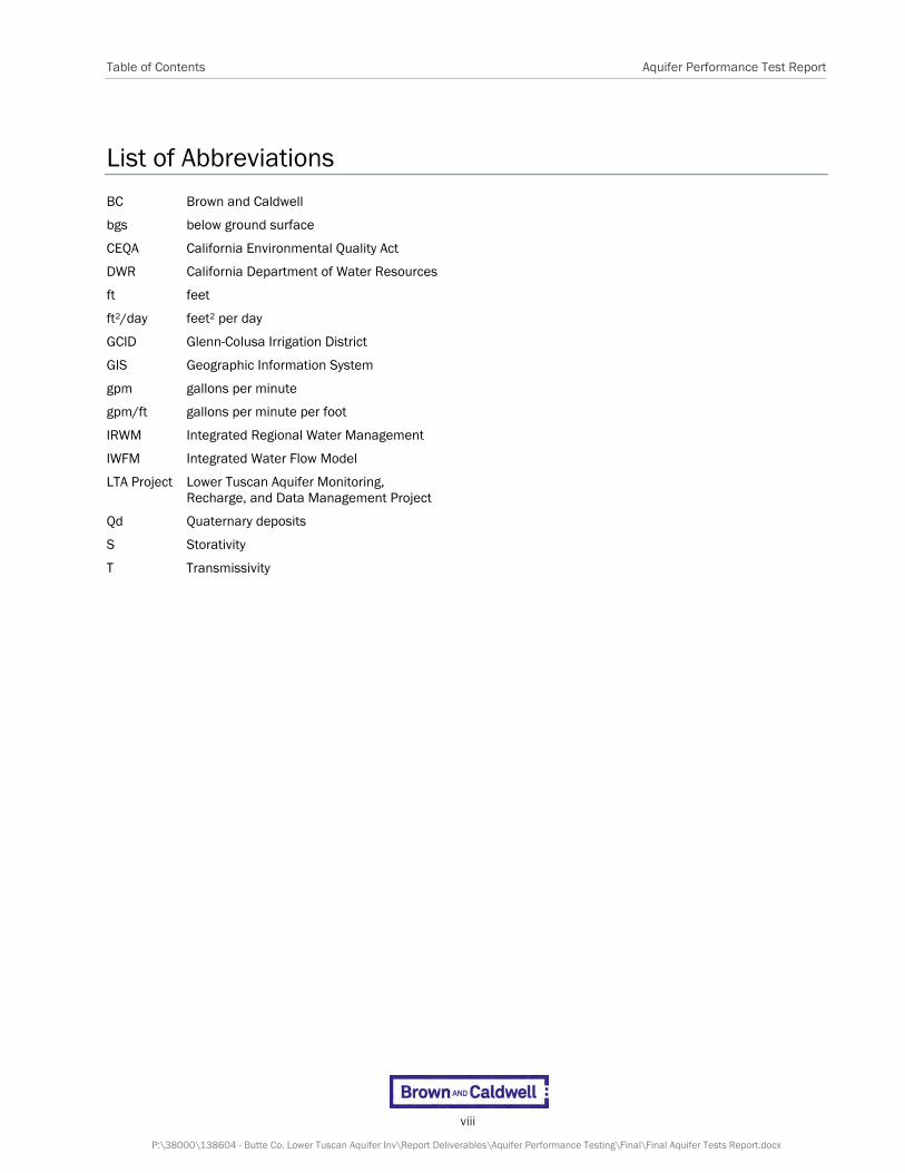
Table of Contents Aquifer Performance Test Report
viii
P:\38000\138604 - Butte Co. Lower Tuscan Aquifer Inv\Report Deliverables\Aquifer Performance Testing\Final\Final Aquifer Tests Report.docx
List of Abbreviations
BC Brown and Caldwell
bgs below ground surface
CEQA California Environmental Quality Act
DWR California Department of Water Resources
ft feet
ft2/day feet2 per day
GCID Glenn-Colusa Irrigation District
GIS Geographic Information System
gpm gallons per minute
gpm/ft gallons per minute per foot
IRWM Integrated Regional Water Management
IWFM Integrated Water Flow Model
LTA Project Lower Tuscan Aquifer Monitoring, Recharge, and Data Management Project
Qd Quaternary deposits
S Storativity
T Transmissivity


1-1
P:\38000\138604 - Butte Co. Lower Tuscan Aquifer Inv\Report Deliverables\Aquifer Performance Testing\Final\Final Aquifer Tests Report.docx
Section 1
Introduction This report presents results from the review of existing aquifer performance tests and completion of three new aquifer performance tests conducted for Task 5, Aquifer Performance Tests, for the Lower Tuscan Aquifer Monitoring, Recharge, and Data Management Project (LTA Project). These activities were conducted in accordance with Attachment Two Section A2.2.5.2 of the County of Butte Contract Number 18050 dated January 31, 2010 between Butte County and Brown and Caldwell (BC). A description of the overall LTA Project is presented in the Initial Study/Proposed Mitigated Negative Declaration prepared by the Butte County, Department of Water and Resource Conservation in May 2010.
1.1 Purpose and Scope Reanalysis of existing aquifer performance tests was conducted to assess if these tests were performed consistent with industry standards whereby the data reported can be used to provide better understanding of the Lower Tuscan Formation aquifer system’s hydraulic performance. Completion of the three new aquifer performance tests were conducted to: 1) collect basic aquifer data including transmissivity (T) and storativity (S) expanded to areas and zones of the LTA not assessed during previous tests; and, 2) to gain a better understanding of the vertical interformational leakage between the Lower Tuscan Formation aquifer system and other hydraulic units. The data developed from these tasks will be used to assess input parameters used for the Butte County Integrated Water Flow Model (IWFM) as part of the Final Report for the LTA Project.
The aquifer performance testing was conducted at existing irrigation and production wells – no new production wells were constructed for this project at three sites as shown on Figure 1-1. For this report the sites are referred to from north to south as the Hackett property, the M&T Ranch, and the Esquon Ranch. The water extracted for each test was used as part of existing irrigation practices and distributed according to normal operating conditions at each location.

Section 1 Aquifer Performance Test Report
1-2
P:\38000\138604 - Butte Co. Lower Tuscan Aquifer Inv\Report Deliverables\Aquifer Performance Testing\Final\Final Aquifer Tests Report.docx
Figure 1-1. Location Map of Aquifer Testing Program of the LTA Recharge Project
The purpose of this report is to summarize results of the review of existing aquifer tests, the methods and procedures used to conduct each of the new tests, and, to present the results of the aquifer performance analysis. A detailed scope of work for the aquifer performance tests was presented in the February 15, 2011 Technical Memorandum No. 3, Aquifer Performance Test Work Plan prepared by BC (Appendix C of First Quarter 2011 Quarterly Report) and included:
Pre-test setup for each aquifer performance test including selection of production wells and equipment used to monitor the test;
Methods used to conduct and monitor the aquifer performance tests; and
Methods used for analysis of the tests.
1.2 Overview of Project The LTA Project consists of seven tasks as follows:
Task 1 – California Environmental Quality Act (CEQA) Initial Study
Task 2 – Technical Steering Committee
Task 3 – Development of Geographic Information System (GIS) Geodatabase

Aquifer Performance Test Report Section 1
1-3
P:\38000\138604 - Butte Co. Lower Tuscan Aquifer Inv\Report Deliverables\Aquifer Performance Testing\Final\Final Aquifer Tests Report.docx
Task 4 – Aquifer Recharge Assessment
Task 5 – Installation of Groundwater Monitoring Wells
Task 6 – Aquifer Performance Testing
Task 7 – Public Outreach
The Tuscan Aquifer system, a regional aquifer of the Sacramento Valley Groundwater Basin, is among the principal water bearing units in Butte County. For this project, the Tuscan Formation has been divided into four units, labeled A through D, as defined by Helly and Hardwood (1985). Units A and B define the LTA, the subject of this study, and units C and D define the Upper Tuscan Aquifer. The approximate extent of the LTA within the project boundaries is shown on Figure 1-1.
Butte County has been awarded grant funds from the California Department of Water Resources (DWR) through Proposition 50 (Water Security, Clean Drinking Water, Coastal and Beach Protection Act of 2002) for implementation of the LTA Project. Included as part of Proposition 50, is the Integrated Regional Water Management (IRWM) Grant Program. Butte County is administering the LTA Project in partnership with the Four County Memorandum o f Understanding Group (Butte, Glenn, Colusa, Tehama, Shasta and Sutter Countiesnow called the Northern Sacramento Valley Integrated Regional Water Management Plan area
The LTA Project is a scientific investigation that will develop data and analytical tools to improve the understanding of the aquifer. Specifically, the LTA Project is a scientific field investigation that seeks to improve the scientific understanding of the properties of the LTA system including:
The physical parameters affecting percolation of surface water to the LTA. The interaction between surface water and the LTA.
Recharge contributions from other aquifers to the LTA.
Measurements of standard aquifer properties and their variability. Identification of natural recharge areas under current hydrologic conditions.
Identification of recharge areas under increase utilization.
How additional pumping may impact the aquifer and surface water.
In addition, the project included development of a comprehensive GIS Geodatabase to store data collected during the duration of the project. As part of the GIS Geodatabase, the project also included development of a field data collection tool that improved the quality of data collected in the field that was incorporated into the geodatabase. Finally, the project included a public outreach program that will heighten public awareness and understanding of the aquifer.
1.3 Overview of Aquifer Testing An aquifer test is a field test where a well is pumped at a controlled rate and water-level response, or drawdown, is measured within the pumping well and one or more surrounding observation wells. Two types of aquifer tests are discussed in this report, step drawdown aquifer tests and constant rate aquifer tests.
A step drawdown aquifer test is a single-well pumping test designed to investigate the performance of a pumping well under controlled variable discharge conditions. In a step drawdown test, the discharge rate, or pumping rate, in the pumping well is increased from an initially low constant rate through a sequence of pumping intervals (steps) of progressively higher constant rates. Each step is typically of equal duration, lasting from approximately 30 minutes to 2 hours. The primary objective of a step drawdown aquifer test is to evaluate well performance criteria such as well loss and well efficiency that can be used to select an appropriate pumping rate for a constant rate aquifer test. The data from a step
Section 1 Aquifer Performance Test Report
1-4
P:\38000\138604 - Butte Co. Lower Tuscan Aquifer Inv\Report Deliverables\Aquifer Performance Testing\Final\Final Aquifer Tests Report.docx
drawdown aquifer test can also be used to provide preliminary estimates of hydraulic properties of an aquifer system such as transmissivity and hydraulic conductivity.
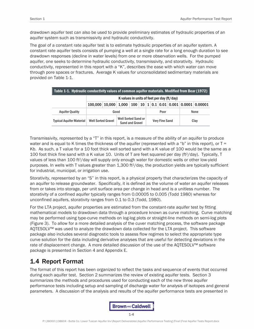
The goal of a constant rate aquifer test is to estimate hydraulic properties of an aquifer system. A constant rate aquifer tests consists of pumping a well at a single rate for a long enough duration to see drawdown responses (decline in water levels) from one or more observation wells. For the pumped aquifer, one seeks to determine hydraulic conductivity, transmissivity, and storativity. Hydraulic conductivity, represented in this report with a “K”, describes the ease with which water can move through pore spaces or fractures. Average K values for unconsolidated sedimentary materials are provided on Table 1-1.
Table 1-1. Hydraulic conductivity values of common aquifer materials. Modified from Bear (1972)
K values in units of feet per day (ft/day)
100,000 10,000 1,000 100 10 1 0.1 0.01 0.001 0.0001 0.00001
Aquifer Quality Good Poor None
Typical Aquifer Material Well Sorted Gravel Well Sorted Sand or
Sand and Gravel Very Fine Sand Clay
Transmissivity, represented by a “T” in this report, is a measure of the ability of an aquifer to produce water and is equal to K times the thickness of the aquifer (represented with a “b” in this report), or T = Kb. As such, a T value for a 10 foot thick well sorted sand with a K value of 100 would be the same as a 100 foot thick fine sand with a K value 10. Units of T are feet squared per day (ft2/day). Typically, T values of less than 100 ft2/day will supply only enough water for domestic wells or other low-yield purposes. In wells with T values greater than 1,300 ft2/day, the production yields are typically sufficient for industrial, municipal, or irrigation use.
Storativity, represented by an “S” in this report, is a physical property that characterizes the capacity of an aquifer to release groundwater. Specifically, it is defined as the volume of water an aquifer releases from or takes into storage, per unit surface area per change in head and is a unitless number. The storativity of a confined aquifer typically ranges from 0.00005 to 0.005 (Todd 1980) whereas for unconfined aquifers, storativity ranges from 0.1 to 0.3 (Todd, 1980).
For the LTA project, aquifer properties are estimated from the constant-rate aquifer test by fitting mathematical models to drawdown data through a procedure known as curve matching. Curve matching may be performed using type-curve methods on log-log plots or straight-line methods on semi-log plots (Figure 3). To allow for a more detailed analysis of the cuver matching process, the software package AQTESOLV™ was used to analyze the drawdown data collected for the LTA project. This software package also includes several diagnostic tools to assess flow regimes to select the appropriate type curve solution for the data including derivative analyses that are useful for detecting deviations in the rate of displacement change. A more detailed discussion of the use of the AQTESOLV™ software package is presented in Section 4 and Appendix E.
1.4 Report Format The format of this report has been organized to reflect the tasks and sequence of events that occurred during each aquifer test. Section 2 summarizes the review of existing aquifer tests. Section 3 summarizes the methods and procedures used for conducting each of the new three aquifer performance tests including setup and sampling of discharge water for analysis of isotopes and general parameters. A discussion of the analysis and results of the aquifer performance tests are presented in
Aquifer Performance Test Report Section 1
1-5
P:\38000\138604 - Butte Co. Lower Tuscan Aquifer Inv\Report Deliverables\Aquifer Performance Testing\Final\Final Aquifer Tests Report.docx
Section 4 and the results of the laboratory analysis of groundwater samples are presented in Section 5 References cited are presented in Section 6. An overall evaluation of these results as they relate to recharge within the LTA and comparison to the Butte County IWFM will be presented in the project Final Report scheduled to be issued in May 2013.

2-1
P:\38000\138604 - Butte Co. Lower Tuscan Aquifer Inv\Report Deliverables\Aquifer Performance Testing\Final\Final Aquifer Tests Report.docx
Section 2
Review of Existing Aquifer Tests As discussed in Section 1.1, the evaluation of existing aquifer performance tests was conducted to assess if these tests were performed consistent with industry standards whereby the data reported can be used to provide better understanding of the Lower Tuscan Formation aquifer system’s hydraulic performance. The Tuscan Project listed six previously conducted tests for consideration. These included:
Sun City, Tehama County (Tehama County)
Deer Creek Irrigation District, Tehama County (DWR) M&T Ranch, Butte County (DWR)
GCID -1, Glenn County (DWR)
Orland/Artois, Glenn County (DWR) Western Canal/Fenn, Butte County (DWR)
The Technical Steering Committee (TSC) was consulted on these and other test for inclusion in this task. Based on input from the TSC, the following four existing aquifer test studies were identified for this task:
A July 1993 report describing aquifer tests conducted as part of the startup of a groundwater extraction system to address impacts associated with the former Koppers Company wood treating facility located in Oroville, California (Dames & Moore, 1993).
A December 1996 report describing two aquifer tests conducted on the M&T Ranch by the DWR as part of a conjunctive use assessment (DWR, 1996).
A March 2009 report discussing aquifer testing of a test production well installed for the Glenn-Colusa Irrigation District (DWR, 2009)
An October 5, 2009 report discussing aquifer testing conducted for a test well installed for the Crystal Geyser Water Company (Crystal Geyser, 2009).
Copies of these reports are provided on CD in Appendix A. A brief summary of the methods and procedures used for each of these tests followed by an assessment of the reported results is provided below.
2.1 1993 Aquifer Testing for startup of Koppers Company Groundwater Extraction System
The results of the aquifer testing conducted for this project are presented in a report entitled “Extraction Well Field Report, Initial Phase Off-Property Groundwater Remedial Action, Koppers Company, Incorporated, Superfund Site” prepared by Dames and Moore (1993). The former Koppers Company is located in south Oroville, California on Baggett Marysville Road (Figure 2-1). The overall report presents results of activities completed during the installation and startup of a groundwater extraction well field installed as part of a remedial action to address impacts to groundwater that migrated offsite of the Koppers’ facility. As part of the system startup phase, step drawdown aquifer tests were conducted for two newly installed extraction wells and a 72-hour constant rate aquifer test was conducted that included monitoring of 19 monitoring wells. Section 2.1.1 summarizes the hydrogeology in the area of tests and brief summaries of the aquifer tests are provided in Sections 2.1.2 and 2.1.3. Section 2.1.4 presents an assessment of the tests compared to industry standards and if the data reported can be used to provide a better understanding of the Lower Tuscan Formation aquifer system’s hydraulic performance.

Section 2 Aquifer Performance Test Report
2-2
P:\38000\138604 - Butte Co. Lower Tuscan Aquifer Inv\Report Deliverables\Aquifer Performance Testing\Final\Final Aquifer Tests Report.docx
Figure 2-1. Site Location Map of Former Koppers Company Facility and
Off-Property Groundwater Extraction System
2.1.1 Hydrogeology
The hydrogeology for the project was developed by Blair and others (1991). In this paper and for the purposes of the remedial investigation conducted as part of the Superfund process, the numerous geologic formations identified in the area were condensed into four units. These units include (from oldest to youngest) the Ione, Tuscan [identified as Mehrten Formation in Blair and others (1991) and Dames and Moore (1993) report], Nomlaki Tuff, and Laguna Formations. In the Oroville area, the Nomlaki Tuff is designated as a member of the Laguna Formation (Busacca, 1982) whereas north of Oroville in the area of the LTA project is designated as part of the Tuscan Formation. The Nomlaki Tuff was isolated as a formal formation for the Koppers Superfund project due to its color, composition, and thickness that made it easily distinguishable in drilling samples from the Laguna and Tuscan Formations. The presence of the Nomlaki Tuff also indicates that the Tuscan Formation in this area is part of the LTA (Brown and Caldwell, 2010). The identification as the LTA in this area is further supported by the presence of metamorphic clasts within the Tuscan Formation of this area as described by Blair and others (1991).
The conceptual hydrogeologic model developed for the site identifies several paleo-valleys formed by the ancestral migration of the Feather River throughout the area. These paleo-valleys juxtapose units of the geologic formations discussed above whereby groundwater aquifers are connected laterally within these areas. These relationships are illustrated in Figure 20 of the Dames and Moore (1993) report that is reproduced below on Figure 2-2.

Section 2 Aquifer Performance Test Report
2-3
P:\38000\138604 - Butte Co. Lower Tuscan Aquifer Inv\Report Deliverables\Aquifer Performance Testing\Final\Final Aquifer Tests Report.docx
Figure 2-2. llustrating Hydrogeologic Conceptual Model Developed for Project. An example of a paleo-valley is shown at the top of diagram
between RI-7/13 and RI-10. Figure 20 from Dames and Moore (1993)

Section 2 Aquifer Performance Test Report
2-4
P:\38000\138604 - Butte Co. Lower Tuscan Aquifer Inv\Report Deliverables\Aquifer Performance Testing\Final\Final Aquifer Tests Report.docx
2.1.2 Step Drawdown Aquifer Tests
Step drawdown aquifer tests were conducted in each of the two extraction wells, designated EW-3 and EW-4, installed for the system. The locations of these wells are shown on Figure 2-3 reproduced from the Dames and Moore (1993) report. Figure 18 from the report (reproduced as Figure 2-4 in this report) presents a generalized geologic cross section that shows the two extraction wells are completed in the Tuscan Formation (referred to as Mehrten Formation in Report). As discussed in Section 2.1.1, the Tuscan Formation in this area is part of the LTA. The approximate thickness of the LTA as measured on Figure 2-3 is 160 feet. A copy of the geologic summary log produced for the two extraction wells is provided in Appendix A. Table 11 from the Dames and Moore (1993) report providing well construction details for these wells along with monitoring wells used for the constant rate aquifer test discussed in Section 2.1.3 is reproduced as Table 2-1.

Aquifer Performance Test Report Section 2
2-5
P:\38000\138604 - Butte Co. Lower Tuscan Aquifer Inv\Report Deliverables\Aquifer Performance Testing\Final\Final Aquifer Tests Report.docx
Figure 2-3. Well Location Map for Extraction Well Aquifer Test Reproduced from Dames and Moore (1993)

Section 2 Aquifer Performance Test Report
2-6
P:\38000\138604 - Butte Co. Lower Tuscan Aquifer Inv\Report Deliverables\Aquifer Performance Testing\Final\Final Aquifer Tests Report.docx
Figure 2-4. Generalized Hydrogeologic Cross Section Showing Construction Details of Extraction Wells Used for Aquifer Test
Figure 18 from Dames and Moore (1993).

Aquifer Performance Test Report Section 2
2-7
P:\38000\138604 - Butte Co. Lower Tuscan Aquifer Inv\Report Deliverables\Aquifer Performance Testing\Final\Final Aquifer Tests Report.docx
Table 2-1. Well construction details for wells used during aquifer testing. Reproduced from Dames and Moore (1993).
Well No. Distance From Pumping Well
(feet)1
Well Casing Diameter (inches)
Screened Interval (feet bgs)
Pump Depth (feet bgs)
Monitoring During Test2
P-2 1980 5 148.5-168.5 - M
RI-8 2520 5 167-197 - M
RI-9 1360 5 161-191 - D,M
RI-10 1325 5 133-163 - D,M
RI-11 2120 8 150-186 - M
RI-12 2180 8 215-255 - M
RI-15 1530 5 178.5-185.5 - M
RI-16A 944 5 72-92 - D,M
RI-16B 956 5 148.5-168.5 - D,M
RI-16C 929 5 178-198 - D,M
RI-16D 943 5 230-250 - D,M
RI-17A 1553 5 94.5-114.5 - D,M
RI-17B 1584 5 136.5-156.5 - D,M
RI-17C 1589 5 192.5-212.5 - D,M
RI-17D 1578 5 236.5-256.5 - D,M
RI-18A 672 5 124-139 - D,M
RI-18B 694 5 165-185 - D,M
RI-19A 896 5 110.5-125.5 - D,M
RI-19B 880 5 160.5-180.5 - D,M
EW-3 - 10 101-201 90 D,M
EW-4 - 10 99.5-199.5 90 D,M
1. Distance from center point between pumping wells EW-3 and EW-4
2. D – datalogger; M - Manual
The step drawdown tests were conducted on February 5 (EW-3) and 8 (EW-4), 1993 and consisted of pumping each well at 200 gallons per minute (gpm), 300 gpm, and 400 gpm for a minimum of 30 minutes at each rate. The wells were not allowed to recover between each step. Using these data, well losses were estimated using the method described by Sheahan (1971) and found to be minimal. The test concluded that the design pumping rate of 300 gpm for the remedial action was feasible within each well. The specific capacity of the wells measured during these tests ranged from 50 to 100 gpm per foot of drawdown.
2.1.3 Constant Rate Pumping Test
A constant rate pumping test was conducted for approximately 72 hours between April 20, 1993 and April 23, 1993 that consisted of pumping both extraction wells EW-3 and EW-4 at 300 gpm. The purpose of this test was to monitor the aquifer’s response to pumping and to use the data to estimate aquifer parameters such as T, S, effective radius (Ro), and capture zone dimensions of the remedial action. Prior to initiating the test, the extractions wells were shut down to allow groundwater to approach static levels. Since the startup of the extraction wells were part of the remedial action for the site, the wells were not shut off after completion of the test and no recovery data was collected.

Section 2 Aquifer Performance Test Report
2-8
P:\38000\138604 - Butte Co. Lower Tuscan Aquifer Inv\Report Deliverables\Aquifer Performance Testing\Final\Final Aquifer Tests Report.docx
In addition to the two extraction wells, water levels were monitored in 11 monitoring well sites as shown on Figure 2-3. Four of these monitoring well sites consist of nested wells with screen intervals completed at various depths throughout the aquifers (see Figure 2-2 and 2-4 for examples). Well construction details for each of these wells are presented in Table 2-1. Water levels were measured using pressure transducers in the two extraction wells and fourteen of the monitoring wells. Site barometric pressure readings were recorded simultaneously by the datalogger. Based on review of barometric changes, correction of data was not required.
Three different techniques were used to analyze the pumping test data. For data analysis purposes, it was assumed that the two pumping wells could be represented by a single pumping well located at the mid-point between EW-3 and EW-4. For most of the observation well data, the Theis curve-matching method for a confined aquifer was used to approximate T and S values. For extraction wells EW-3 and EW-4, the Jacob straight line method was used to calculate T values. The straight line matches and calculations of T from this analysis are reproduced in Figures 2-5 and 2-6. The distance versus drawdown method was also used to calculate T and S, as well as the Ro using elapsed times of 100 minutes and 1,000 minutes as shown on Figures 2-7 (100 minutes) and 2-8 (1,000 minutes).
Figure 2-5. Time Drawdown Curve and Cooper-Jacob Straight Line Solution for Extraction Well EW-3
Reproduced from Dames and Moore (1993)
Aquifer Performance Test Report Section 2
2-9
P:\38000\138604 - Butte Co. Lower Tuscan Aquifer Inv\Report Deliverables\Aquifer Performance Testing\Final\Final Aquifer Tests Report.docx
Figure 2-6. Time Drawdown Curve and Cooper-Jacob Straight Line Solution for Extraction Well EW-4
Reproduced from Dames and Moore (1993)
Figure 2-7. Distance Drawdown Plot at Time Equals 100 Minutes
Reproduced from Dames and Moore (1993)

Section 2 Aquifer Performance Test Report
2-10
P:\38000\138604 - Butte Co. Lower Tuscan Aquifer Inv\Report Deliverables\Aquifer Performance Testing\Final\Final Aquifer Tests Report.docx
Figure 2-8. Distance Drawdown Plot at Time Equals 1,000 Minutes
Reproduced from Dames and Moore (1993)
The Dames and Moore (1993) report states that drawdown data indicated that all monitoring wells monitored for the test responded to pumping except for well RI-16A (Figure 2-3). As illustrated on Figure 2-4, this well is completed within the Nomlaki Formation overlying the LTA in this area suggesting that the shallow aquifer zone monitored by this well is not in hydraulic connection with the LTA. Review of the drawdown curve for this well does suggest the well responded to pumping during later portions of the test possible indicating a leakage response between the two aquifers. Estimates of T using the methods described above varied from 16,100 feet2 per day (ft2/day) to 26,300 ft2/day with an average of 20,140 ft2/day and values of S varied 0.0002 to 0.00044 with an average value of 0.00028. The Ro using the distance versus drawdown method was approximately 3,000 feet after 100 minutes of pumping and 4,000 feet after 1,000 minutes of pumping. Inspection of the drawdown curves indicates that after 1,000 minutes of pumping, drawdowns appear to be reaching equilibrium.
Using the capture zone equations presented by McWhorter and Sunada (1977) and Javandel and Tsang (1986), estimates of the capture zone width and stagnation point for a confined aquifer after reaching equilibrium were calculated. The equation is:
Ymax = Q/Ti
Where Ymax is the maximum width of the capture zone far upgradient of the pumping wells, Q is the pumping rate and i is the hydraulic gradient. Capture zone width at the pumping well can be estimated using the relationship:
Ywell = Ymax/2
The stagnation point X, the downgradient location where the particle velocity caused by pumpage in the extraction well equals the velocity imparted by regional flow, is calculated using the relationship:
X = Ywell/π

Aquifer Performance Test Report Section 2
2-11
P:\38000\138604 - Butte Co. Lower Tuscan Aquifer Inv\Report Deliverables\Aquifer Performance Testing\Final\Final Aquifer Tests Report.docx
These parameters were calculated using the following values obtained from the aquifer test:
Q = 600 gpm T= 20,140 ft2/day i = 0.001
Using these values Ymax is 5,375 feet, Ywell is 2,878 feet, and X is 913 feet.
2.1.4 Usability of Data
Software packages such as AQTESOLV™ were not available in 1993 when this aquifer test was conducted and curve matching was conducted by visual assessments. As such, the drawdown curves produced for this project were only evaluated using the Theis (1935) solution for unsteady flow to a fully penetrating well in a confined aquifer that assumes a line source for the pumping well and therefore ignores wellbore storage. This solution also does not account for leakage through an aquitard. The conceptual model developed for this site is very similar to the conceptual model developed for the aquifer test conducted at the Esquon Ranch (Section 3.3) whereby the LTA monitored for the aquifer test is not in hydraulic connection with a shallow aquifer and leakage occurs through the aquitards. Using the Theis (1935) solution for drawdown curves produced from monitoring wells during the Esquon Ranch, the T values were between 23,800 ft2/day to 20,900 ft2/day consistent with the average value of 20,140 ft2/day calculated for this test. However, as discussed in Section 3.3, the more appropriate solution to use based on the conceptual model is Moench (1985). This method can be used to assume that a constant-head source aquifer supplies leakage across overlying and/or underlying aquitards that is consistent with observation of wells completed in different aquifers during the Esquon aquifer tests. The curve fits using this solution for the Esquon tests provided very good fits and the T values calculated were between 6,653 ft2/day and 8,088 ft2/day. Similar T values would be expected for the Koppers’ aquifer test if the Moench (1985) solution was used for these data although values calculated from the Theis solution are within the same order of magnitude and would not significantly affect the results of groundwater models developed from these data. The average S value of 0.00028 calculated for the Koppers’ test is also consistent with the values calculated for the Esquon Ranch where the average S value is 0.00034. The capture zone analysis provided from this testing can be used to provided initial assessments of the zone of influence (distance from pumping well) that would be affected by pumping of a well at specific pumping rate
Of more significant importance from this test was the development of the site conceptual hydrogeologic model. This detailed model was developed from lithologic samples collected continuously during drilling that were used to produce detailed geologic boring logs that included the identification of formation boundary’s, relative differences in water production between zones, and vertical differences in water quality. The methods of Blair and others (1991) used for the LTA project for developing the criteria for identifying formation boundaries from lithologic samples collected during the drilling of monitoring wells (Brown and Caldwell, 2010) is based on the data collected from the Kopper’s project. As illustrated on Figure 2-2, this detailed analysis showed that deposition of materials from the ancestral migration of the Feather River formed large paleo-valleys where aquifer materials of the LTA are juxtaposed against aquifer zones developed within other units. This juxtaposition results in groundwater flowing laterally from one aquifer unit (Laguna Formation) to other aquifer units (LTA and/or Ione). This type of lateral flow between the LTA aquifer unit and other formations is further illustrated below on Figure 2-9 reproduced from Blair and others (1991). The arrows presented on the figure represent the movement of groundwater and show the lateral movement between aquifer units (as indicated in Section 2.1.1, Blair and others (1991) refer to the LTA as the Mehrten Formation).

Section 2 Aquifer Performance Test Report
2-12
P:\38000\138604 - Butte Co. Lower Tuscan Aquifer Inv\Report Deliverables\Aquifer Performance Testing\Final\Final Aquifer Tests Report.docx
Figure 2-9. Arrows presented on cross section represent the direction of groundwater flow and illustrate the lateral
movement of groundwater between the different aquifer formations. Lower Tuscan Formation designated as Mehrten Formation in report.
Figure 9a from Blair and Others (1991).
It is anticipated that this type of relationship exists throughout the LTA and future studies should focus on developing the data to assess these conditions throughout the basin.
Based on review of the data presented in the above sections, the aquifer tests conducted for this project were performed in accordance with industry standards of the time and the data reported can be used to provide a better understanding of the Lower Tuscan Formation aquifer system’s hydraulic performance.
2.2 1996 M&T Chico Ranch Aquifer Test The results of the aquifer test conducted for this project are presented in a memorandum prepared by the DWR in December 1996 entitled M&T Chico Ranch Conjunctive Use Investigation, Phase III (DWR, 1996). The M&T Chico Ranch is located in western Butte County and consists of about 8,300 acres, bordered by the Sacramento River to the west, Big Chico Creek to the north, and Ord Ferry Road to the south. This ranch is also the location of one of the aquifer tests conducted for the LTA project as discussed in Section 3.3. Figure 2-10 shows the location of the well used for the test discussed in this section as well as the pumping well used for the LTA project.
The report presents results of aquifer tests conducted in June 1995 and May 1996. The June 1995 aquifer test was conducted in a then recently installed production well completed within the LTA. The primary objective of this aquifer test was to assess the aquifer performance of the LTA in this area and the production/efficiency of the newly installed well. Aquifer testing consisted of step-drawdown tests and a 45 hour constant rate aquifer test. A secondary purpose of the constant rate aquifer test was to assess possible interconnection between shallow and deep aquifer zones and included recording drawdown in seven surrounding monitoring wells. A pumping rate of 1,650 gpm was used for the constant rate test.

Aquifer Performance Test Report Section 2
2-13
P:\38000\138604 - Butte Co. Lower Tuscan Aquifer Inv\Report Deliverables\Aquifer Performance Testing\Final\Final Aquifer Tests Report.docx
Figure 2-10. Location of Pumping Well used for LTA Project (PW-MT-1) and the DWR M&T Aquifer Test (PW-MT-4)
Findings from the June 1995 test concluded that there was reduced well efficiency of the newly installed well due to inadequate well development or less than optimum gravel pack size. Based on these findings, a new pump was installed within the production well and the well was redeveloped in April 1996. After development, the May 1996 aquifer test was conducted that consisted of a step-drawdown test on the production well and a 30 hour constant rate aquifer test. The constant rate aquifer test consisted of pumping the production well at 3,000 gpm and recording drawdown in five surrounding monitoring wells.
Section 2.2.1 summarizes the hydrogeology in the area of tests and brief summaries of the aquifer tests are provided in Sections 2.2.2 and 2.2.3. Section 2.2.4 presents an assessment of the tests compared to industry standards and if the data reported can be used to provide a better understanding of the Lower Tuscan Formation aquifer system’s hydraulic performance.
2.2.1 Hydrogeology
The DWR (1996) report states that earlier reports identified a laterally extensive and potentially productive water-bearing zone beneath the M&T Chico Ranch within the “lower-confined” Tuscan Formation aquifer. Based on screen intervals completed for this project, this aquifer occurs between approximately 730 feet bgs to 1,000 feet bgs. The DWR (1996) report indicated that earlier data collected by DWR in 1993 ed showed that the deeper aquifer system is overlain by significant low permeability units (clay units) that separate this aquifer from

Section 2 Aquifer Performance Test Report
2-14
P:\38000\138604 - Butte Co. Lower Tuscan Aquifer Inv\Report Deliverables\Aquifer Performance Testing\Final\Final Aquifer Tests Report.docx
shallower aquifers within both the Tuscan Formation and younger formations whereby drawdown (lowering of water levels) would be minimized in the shallow systems from pumping in the deeper aquifer. As discussed in Section 4.3.1 and illustrated on Figure 4-10, the occurrence of this deeper aquifer at the approximate depths stated was confirmed during the drilling of the groundwater monitoring well completed for the LTA project on the M&T Ranch. Figure 4-10 also shows shallower aquifers within the upper Tuscan Aquifer (350 feet bgs to 400 feet bgs) and younger Quarternary Deposits (20 feet bgs to 100 feet bgs).
2.2.2 June 1995 Aquifer Testing
For this aquifer test, a 1,018 foot monitoring well, designated 24B01, and 950 foot test production well, designated 24B02, were installed. Production well 24B02 was also monitored for the aquifer test conducted for the LTA project at the M&T Ranch and was designated PW-MT-4 (Section 3.2). The monitoring well is screened from 820 to 840 feet bgs whereas the production well is screened from 760 to 920 feet bgs. Aquifer tests included performance of a step-drawdown test and constant rate test. During these tests, groundwater level measurements were collected using a steel tape and electronic sounder. Pumping rates were determined with an ultrasound flow meter and adjusted using partially-full-pipe calculations.
The step-drawdown test consisted of pumping well 25B02 for three one-hour steps at incrementally increasing pumping rates of 800 gpm, 1,300 gpm, and 1,740 gpm. During this pumping, drawdown was recorded in the pumping well as well as monitoring well 24B01. The primary purpose of the step drawdown test was to provide the information necessary for design of an appropriate constant-discharge aquifer test but also provided preliminary estimates of aquifer transmissivity. Figure 3 from this report presented the drawdown curves within the pumping well for this test and the estimated specific capacities and is reproduced below in Figure 2-11. Using the Theis recovery method, a preliminary estimate of the T for this aquifer was 8,020 ft2/day.
Figure 2-11. Time Drawdown Plot for 1995 Step Drawdown Test
Reproduced from DWR (1996)
The constant rate aquifer test started on June 14, 1995 and continued for approximately 45 hours. Based on the results of the step-drawdown test, the pumping rate for the test production well 24B02 was set at 1,650 gpm. As stated in the DWR (1996) report, the objective of this aquifer test was to provide more accurate estimates of aquifer T and S and to examine possible interconnections between the deeper aquifer and shallow aquifers. During the test, drawdown was recorded in the pumping well and seven surrounding observation wells. For the pumping well and the newly installed monitoring well 24B01, drawdown was recorded frequently during the test. For the remaining six observation wells, drawdown measurements were only recorded at approximately
Aquifer Performance Test Report Section 2
2-15
P:\38000\138604 - Butte Co. Lower Tuscan Aquifer Inv\Report Deliverables\Aquifer Performance Testing\Final\Final Aquifer Tests Report.docx
6, 23, and 44 hours after startup of the test. Observation wells ranged from 191 feet to 8,200 feet from the pumping well as shown on Figure 7 of the DWR (1996) report reproduced below as Figure 2-12. With the exception of the newly installed monitoring well 24B01, the observation wells were screened within shallower zones than the pumped well with total depths ranging from 54 feet bgs (well 23J01 approximately 5,800 feet from pumping well) to 640 feet bgs (well 07l01 approximately 7,300 feet from pumping well).
Figure 2-12. Location Map Showing Location of Wells Monitored during 1995 Aquifer Test
Figure 7 from DWR (1996).
Aquifer analysis was conducted using the software package AQTESOLV™ and the drawdown data from observation well 24B01. AQTESOLV™ is the same package used for analysis of aquifer tests conducted for the LTA project as discussed in Section 3. Solutions used for analysis included the confined aquifer solutions of Theis and Cooper-Jacobs and the leaky confined aquifer solution of Moench. From this analysis T values ranged from 9,940 ft2/day (Moench solution) to 10,329 ft2/day (Theis solution) and S values ranged from 0.00008 (Moench solution) to 0.00027 (Cooper-Jacobs).
The DWR (1996) report indicated that the drawdown curve for the pumping well appeared characteristic of a well pumping from a leaky aquifer or from a well intersecting a recharge source. In addition, this report states that based on response from observation wells completed within shallower aquifers that there is no apparent connection with these zones and the deeper aquifer where pumping occurred. The DWR (1996) report also

Section 2 Aquifer Performance Test Report
2-16
P:\38000\138604 - Butte Co. Lower Tuscan Aquifer Inv\Report Deliverables\Aquifer Performance Testing\Final\Final Aquifer Tests Report.docx
concluded that the pumping well efficiency was low and that additional well development should be conducted and another aquifer test conducted at higher pumping rates.
2.2.3 May 1996 Aquifer Testing
Based on the recommendations from the June 1995 aquifer test, the production well used for this test was redeveloped on April 29, 1996. Based on estimated specific capacity during this development, DWR concluded that the initial well development in 1995 was probably adequate. After well development, another step-drawdown test was conducted that consisted of pumping the production well for three one-hour steps at successive rates of 1,250 gpm, 2,050 gpm, and 3,000 gpm. Using the Theis recovery formula, the estimated T for this test was 7,085 ft2/day. Using this information, a 30-hour constant rate test was started on May 6, 1996. This test consisted of pumping the production well 24B02 at a constant rate of 3,000 gpm and recording drawdown in five surrounding monitoring wells including the test well installed for the June 1995 test, 24B01 (see Figure 2-12 for locations).
Figure 2-13 reproduces the drawdown graph for monitoring well 24B01 and shows that the total drawdown in this well was approximately 43 feet with 80 percent recovery two hours after shutdown of the production well. As with the June 1995 aquifer test, observation well 13H01 (completed less than 100 feet bgs) located about 2,700 feet northeast of pumping well, showed no changes in water levels during the aquifer test. Response to pumping from the other three observation wells could not be assessed because observation well 23J01 began pumping two hours into the test.
Figure 2-13. Time Drawdown Graph for Monitoring Well 24B01 During 1996 Constant-Discharge Aquifer Test
Reproduced from DWR (1996)
As with the previous aquifer test, aquifer analysis was conducted using the software package AQTESOLV™ and the drawdown data from observation well 24B01. Solutions used for analysis included the confined aquifer solutions of Theis and Cooper-Jacobs and the leaky confined aquifer solution of Moench. An independent hand analysis not using the AQTESOLV™ software was also conducted using the Cooper-Jacob straight line solution. From this analysis T values ranged from 9,213 ft2/day (Moench solution) to 10,055 ft2/day (Cooper-Jacobs hand solution) and S values ranged from 0.000096 (Cooper Jacobs hand solution) to 0.000027 (all other solutions). These values are consistent with the June 1995 aquifer test. DWR also concluded that the time-drawdown data was more characteristic of a confined aquifer rather than a leaky confined aquifer.
DWR assessed two proposed production well designs to assess potential drawdown related impacts to surrounding groundwater users near the M&T Ranch. The two proposed well designs included a composite well screened within both the intermediate aquifer zone and deep aquifer zone (300 to 900 feet bgs) and a well

Aquifer Performance Test Report Section 2
2-17
P:\38000\138604 - Butte Co. Lower Tuscan Aquifer Inv\Report Deliverables\Aquifer Performance Testing\Final\Final Aquifer Tests Report.docx
screened only within the deep aquifer zone (760 to 920 feet bgs). The analysis was conducted using the aquifer parameters calculated during the May 1996 aquifer tests and the computer software package WTAQ2 (Barlow and Moench, 2011). WTAQ2 simulates axial-symmetric flow to a well pumping from a confined or unconfined (water-table) aquifer and calculates dimensionless or dimensional drawdowns.
For the deep aquifer zone, a T value of 10,026 ft2/day and specific capacity of 23 gallons per minute per foot (gpm/ft) were used for the analysis. For the composite well, a T value of 16,710 ft2/day and specific capacity of 30 gpm/ft were used. DWR also stated that they calculated drawdowns assuming a water-table system throughout even though the proposed production wells would be completed within confined aquifers. This approach was taken because sufficient stress within the confined system could result in groundwater drawdown within the unconfined aquifer. The results of this analysis are reproduced in Table 2-2 and assumed continuous pumping for 90 days.
Table 2-2. Summary of DWR WTAQ2 Analysis for Potential Drawdown Impacts Related to
Operation of Proposed Production Wells
Reproduced from DWR (1996).
2.2.4 Usability of Data
As discussed in the introduction to Section 2.2, the production well (240B2) used for this aquifer test was monitored as part of the aquifer test conducted for the LTA project. For the LTA project this well was labeled PW-4 (Section 3.2). The production well used for the LTA project is screened within the intermediate aquifer (approximately 340 to 390 feet bgs) described in the DWR (1996) report as opposed to the deep aquifer (760 to 920 feet bgs) screened by the production well used for the DWR aquifer test. Only one well appeared to be screened within the intermediate aquifer zone (well 07L01, Figure 2-14) for the DWR test but was located over 1-mile from the production well and showed no response to pumping. Based on this data, the DWR concluded that there was no hydraulic connection between the two aquifers but did suggest that at higher pumping rates and longer sustained pumping, there could be a connection. For the May 1995 aquifer test, the DWR stated that the drawdown curve for the pumping well appeared characteristic of a well pumping from a leaky aquifer or from a well intersecting a recharge source.
As part of the LTA aquifer test, monitoring wells were placed within the intermediate aquifer zone, aquitard material between the intermediate aquifer and deep aquifer (screened from 570 to 590 feet bgs), and within the deep aquifer zone. As discussed in Section 3.2, the results of the LTA aquifer test clearly showed a hydraulic

Section 2 Aquifer Performance Test Report
2-18
P:\38000\138604 - Butte Co. Lower Tuscan Aquifer Inv\Report Deliverables\Aquifer Performance Testing\Final\Final Aquifer Tests Report.docx
connection between the intermediate and deep aquifer zones with significant leakage occurring through the aquitard.
To further assess the results of the DWR (1996) aquifer tests, reported water level data from the May 1996 test was entered into the current version of AQTESOLV™ and analyzed following the procedures used for the LTA project (Section 4). This analysis uses a series of diagnostic flow plots that aid in selecting the appropriate aquifer solutions methods for assessing the aquifer test data. The detailed analysis using these plots for the DWR May 1996 aquifer test is presented in Appendix B and summarized below.
As stated in the AQTESOLV™ User Manual (2007), derivative analysis is an invaluable tool for diagnosing a number of distinct flow regimes. Examples of flow regimes that one may discern with derivative analysis include infinite-acting radial flow, wellbore storage, linear flow, bilinear flow, inter-porosity flow and boundaries. The derivative analysis of well 24B01 for the DWR May 1996 test is presented on Figure 2-14. Areas where the derivative plot reaches a plateau indicate infinite acting radial flow and are portions of the drawdown curve appropriate for the Cooper-Jacob straight line method to calculate transmissivity and storativity values of the aquifer. As seen on Figure 2-14, a plateau of the derivative plot occurs between about 5 minutes and 20 minutes after startup of pumping. Figure 2-15 shows estimates of T and S using the Cooper-Jacob straight line method over this portion of the curve.
Figure 2-14. Derivative (Blue) and Drawdown Curves (Red) for Well 24B01 during May 1996 DWR Aquifer Test
DWR Test
10-1
100
101
102
103
10410
0
101
102
Time (min)
Dis
pla
cem
ent (
ft)
Obs. Wells
24B01

Aquifer Performance Test Report Section 2
2-19
P:\38000\138604 - Butte Co. Lower Tuscan Aquifer Inv\Report Deliverables\Aquifer Performance Testing\Final\Final Aquifer Tests Report.docx
Figure 2-15. Cooper Jacob Straight Solution for Well 24B01 during May 1996 DWR Aquifer Test
As seen on Figure 2-15 the estimated T and S values for this test are 7,138 ft2/day and 0.00022, respectively. DWR’s estimate T and S values using the Cooper-Jacob solution was 9,960 ft2/day and 0.000027, respectively. The shape of the derivative curve can also be used to interpret flow regions. As shown on Figure 2-14, after the plateau discussed above, the derivative curve appears to start plunging toward zero. This behavior represents a single infinite recharge (constant-head) boundary or a leaky confined aquifer with an incompressible aquitard and constant-head source aquifer. Both of these interpretations are consistent with the interpretations suggested by DWR during the June 1995 test and the LTA aquifer test conducted within the intermediate aquifer.
Based on the derivative analysis discussed above, the Moench (1985) solution was selected for analysis of the drawdown curve. This is the same method selected by DWR for the May 1996 aquifer test that provides a solution for unsteady flow to a fully penetrating, finite-diameter well with wellbore storage and wellbore skin in a homogeneous, isotropic leaky confined aquifer. In AQTESOLVE, there are three configurations for simulating a leaky confined aquifer with aquitard storage for this method as follows: Case 1 assumes constant-head source aquifers supply leakage across overlying and underlying aquitards.
Case 2 replaces both constant-head boundaries in Case 1 with no-flow boundaries
Case 3 replaces the underlying constant-head boundary in Case 1 with a no-flow boundary.
The Case 3 scenario was selected for analysis of the May 1996 test and is presented on Figure 2-16.
DWR Test
10-1
100
101
102
103
1040.
8.
16.
24.
32.
40.
Adjusted Time (min)
Dis
pla
cem
ent (
ft)
Obs. Wells
24B01
Aquifer Model
Confined
Solution
Cooper-Jacob
Parameters
T = 7138.2 ft2/dayS = 0.0002178
Section 2 Aquifer Performance Test Report
2-20
P:\38000\138604 - Butte Co. Lower Tuscan Aquifer Inv\Report Deliverables\Aquifer Performance Testing\Final\Final Aquifer Tests Report.docx
Figure 2-16. Moench (1985) solution for well 24B01 during May 1996 aquifer test. Curve fits for drawdown (red) and
derivative plot (green) area shown in blue.
As seen on this figure, very good curve fits (blue lines) were obtained for both the drawdown curve and derivative plot indicating that this was an appropriate solution for the test. T and S values calculated using this solution are 5,817 ft2/day and 0.00018, respectively. Using this same solution, DWR calculated T and S values of 9,213 ft2/day and 0.000027, respectively. Using the more detailed analysis of data as conducted for the LTA project, the T and S values calculated for this report are believed to be more accurate.
Neuman and Witherspoon (1969) derived a solution for unsteady flow to a fully penetrating well in a confined two-aquifer system. The solution assumes a line source for the pumped well and therefore neglects wellbore storage. This method allowed an assessment of calculated T and S values within the intermediate aquifer zone and K values for the aquitard. Figure 2-17 presents the results of this analysis for well 24B01.
DWR Test
10-1
100
101
102
103
10410
0
101
102
Time (min)
Dis
pla
cem
ent (
ft)
Obs. Wells
24B01
Aquifer Model
Leaky
Solution
Moench (Case 3)
Parameters
T = 5817.1 ft2/dayS = 0.0001826r/B' = 0.1073ß' = 0.05872r/B" = 0.ß" = 0.Sw = 0.r(w) = 1.167 ftr(c) = 0.6667 ft

Aquifer Performance Test Report Section 2
2-21
P:\38000\138604 - Butte Co. Lower Tuscan Aquifer Inv\Report Deliverables\Aquifer Performance Testing\Final\Final Aquifer Tests Report.docx
Figure 2-17. Neuman-Witherspoon (1969) solution for well 24B01 during May 1996 aquifer test.
Curve fits for drawdown (red) and derivative plot (green) area shown in blue.
As seen on this figure, the T and S values calculated for the deep aquifer using this solution are consistent with those calculated using the Moench (1985) solution. For the intermediate aquifer, this solution calculated a T value (T2 on Figure 2-17) of 21,125 ft2/day and an S value of 0.00001. During the LTA project, the calculated T and S values for the intermediate aquifer using the Moench (1985) solution ranged from 11,550 ft2/day to 20,680 ft2/day and 0.00045 to 0.0003, respectively. As seen by these results, T values from the LTA project and analysis of the DWR (1996) results are relatively comparable for the intermediate aquifer zone. The K value calculated for the aquitard between the two aquifers is 1.531 ft/day (Appendix A).
Based on review of the data presented in the above sections, the aquifer tests conducted for this project were performed in accordance with industry standards of the time and the data reported can be used to provide a better understanding of the Lower Tuscan Formation aquifer system’s hydraulic performance.
2.3 March 2009 Glenn-Colusa Irrigation District Test-Production Well Installation and Aquifer Testing
In 2005, the Glenn-Colusa Irrigation District (GCID) began a three year project that included the installation of a test production well, quadruple-completion observation well, and performance of constant rate aquifer test. The purpose of the project was to further characterize the lower aquifer system in the area and provide recommendations for future investigations. The results of this project are presented in a March 2009 report prepared by DWR entitled Glenn-Colusa Irrigation District Test-Production Well Installation and Aquifer Testing (DWR, 2009). Figure 1 from this report, reproduced as Figure 2-18, shows the location of these wells completed near County Road 203 in Glenn County.
DWR Test
10-1
100
101
102
103
10410
0
101
102
Time (min)
Dis
pla
cem
ent (
ft)
Obs. Wells
24B01
Aquifer Model
Leaky
Solution
Neuman-Witherspoon
Parameters
T = 5194.2 ft2/dayS = 0.000214r/B = 0.1936ß = 0.07165T2 = 2.125E+4 ft2/dayS2 = 1.0E-5

Section 2 Aquifer Performance Test Report
2-22
P:\38000\138604 - Butte Co. Lower Tuscan Aquifer Inv\Report Deliverables\Aquifer Performance Testing\Final\Final Aquifer Tests Report.docx
Figure 2-18. Location Map for GCID Test Production Well and Observation Well
Figure 1 from DWR (2009)
Aquifer testing included a 12-hour step-drawdown test, a 24-hour constant rate aquifer test, and a 28-day constant rate aquifer test. Flow rates for these tests ranged from 1,500 gpm to 6,000 gpm.
Section 2.3.1 summarizes the hydrogeology in the area of tests and brief summaries of the aquifer tests are provided in Sections 2.3.2 and 2.3.3. Section 2.3.4 presents an assessment of the tests compared to industry standards and if the data reported can be used to provide a better understanding of the Lower Tuscan Formation aquifer system’s hydraulic performance.
2.3.1 Hydrogeology
The geologic borehole logs produced for this project are reproduced in Appendix B. As shown on these logs, three main aquifer-bearing geologic formations were logged by DWR in the test-production and observation well boreholes: the Tuscan Formation, Tehama Formation, and Stony Creek Fan alluvium. Figure 2-19, reproduced from DWR (2009) shows the surface and approximate subsurface extent of these formations in the Sacramento Valley.

Aquifer Performance Test Report Section 2
2-23
P:\38000\138604 - Butte Co. Lower Tuscan Aquifer Inv\Report Deliverables\Aquifer Performance Testing\Final\Final Aquifer Tests Report.docx
Figure 2-19. Surface and Subsurface Extent of Tuscan, Tehama, and Stony Creek Fan Alluvium
Reproduced from DWR (2009)
DWR (2009) also states that the fresh-to-brackish Upper Princeton Valley fill underlies the Tuscan and Tehama Formations in the study area. However, as discussed in Section 4.1, as defined by Redwine (1972), the Princeton Submarine Valley System is a morphological feature of the ancestral Sacramento River Basin and contains the geologic formations described within the Sacramento Valley. For example, the Ione Formation is used by Redwine to separate the lower and upper Princeton Valley fills and the Lovejoy Basalt is interpreted to represent the rimrock of the upper Princeton Valley Fill.
As shown on the geologic well logs (Appendix B) and summarized on Table 2-3, the test production well is completed within the Tuscan Formation and quadruple-completed observation wells has screen intervals within the Stony Creek Fan, Tehama Formation, and Tuscan Formation.
Section 2 Aquifer Performance Test Report
2-24
P:\38000\138604 - Butte Co. Lower Tuscan Aquifer Inv\Report Deliverables\Aquifer Performance Testing\Final\Final Aquifer Tests Report.docx
Table 2-3. Well Construction Details for Newly Installed Test Production and Nested Observation Well
Well State Well I.D. Well Diameter
(inches) Screen Interval
(feet bgs) Geologic Formation
Test Production Well 22N02WO2JOO1M 20 800-820, 840-870,
900-1,240, 1,270-1,300 Tuscan
Observation Well 22N02W01N004M 2.5 71-81 Stony Creek Fan
Observation Well 22N02W01N003M 2.5 209-219, 358-368 Tehama
Observation Well 22N02W01N002M 2.5 699-709 Tehama/Tuscan
Observation Well 22N02W01N001M 2.5 813-823, 1040 to 1050 Tuscan
Other wells used for the 28-day constant rate aquifer test are screened in one or more of these formations as discussed in Section 2.3.3.
2.3.2 Step Drawdown and 24-Hour Constant Rate Aquifer Tests
A step drawdown aquifer test was conducted in newly installed test production well during December 2005. As discussed above, the well is completed within the Tuscan Formation with an approximate thickness of 500 feet (see geologic well log, Appendix B). The step drawdown tests consisted of pumping the well successive rates of 1,500 gpm, 3,000 gpm, 4,000 gpm, 5,000 gpm, and 6,000 gpm for intervals between 100 and 150 minutes. The well was not allowed to recover between each step.
Within 24-hours after completion and using the data generated from the step test, a 24-hour constant rate aquifer test was conducted at a pumping rate of 5,000 gpm. Because the nearby nested observation well (N001M through N004M) had not yet been installed, groundwater levels were only measured in the test production well during these tests. The primary objective of the step drawdown and 24-hour constant rate aquifer tests was to determine the highest flow rate at which the test production well could operate efficiently during the 28-day constant rate aquifer test.
Time versus drawdown plots for the step drawdown and 24-hour constant rate tests are shown on Figures 2-20 and 2-21, respectively. Specific capacities measured during the step drawdown test ranged from 27.2 gpm per foot of drawdown (6,000 gpm) to 33.6 gpm per foot of drawdown (1,500 gpm). Using the Jacob Straight Line method, DWR (2009) calculated a T of 5,437 ft2/day from the 24-hour constant discharge test (solution shown on Figure 2-22). The calculated hydraulic conductivity (K) value based on an aquifer thickness of 480 feet is 11.14 ft/day typical for silty to clean sands (Table 1-1).

Aquifer Performance Test Report Section 2
2-25
P:\38000\138604 - Butte Co. Lower Tuscan Aquifer Inv\Report Deliverables\Aquifer Performance Testing\Final\Final Aquifer Tests Report.docx
Figure 2-20. Time Drawdown Plot for 12-Hour Step-Drawdown Aquifer Test
Reproduced from DWR (2009)
Figure 2-21. Time Drawdown Plot and Jacob Straight Line Solution for Test Production Well
During 24-Hour Constant-Discharge Aquifer Test Reproduced from DWR (2009)

Section 2 Aquifer Performance Test Report
2-26
P:\38000\138604 - Butte Co. Lower Tuscan Aquifer Inv\Report Deliverables\Aquifer Performance Testing\Final\Final Aquifer Tests Report.docx
2.3.3 28-Day Constant Rate Aquifer Test
The 28-day constant rate aquifer test was conducted between April 18, 2007 and May 16, 2007 that consisted of pumping the test production well. Pumping started at approximately 3,000 gpm then was increased to 3,500 gpm one hour into the test due to cavitation problems at 3,000 gpm. The purpose of this test was to better estimate the hydrogeologic properties of the deep aquifer system (Tuscan Formation), evaluate aquifer interconnections, and identify possible aquifer boundary conditions. Groundwater levels during the test were recorded in the test production well and 46 observation wells, including the 4 wells of the quadruple completion well installed for the test. Many of the other observations are multi-completion observation wells similar in construction to the quadruple completed observation well installed for this project.
Ten of the observation wells are completed within the Tuscan Aquifer system pumped by the production well. Table 2-4 reproduced Table 5 from the DWR (2009) report summarizing well construction details and approximate distance from the pumping well for each of these ten observations wells. Figure 2-22 shows the location of the test well and 46 observation wells used for the test.
Table 2-4. Well Construction details of test production and observation wells used for 28-day constant discharge test. Reproduced Table 5 from DWR (2009).
Groundwater levels in the test well were measured at 1-minute intervals until two days after shutdown of the pumping well (May 18, 2007) at which time water levels were recorded every 10 minutes until May 30, 2007. Groundwater levels within the observation wells were recorded hourly throughout the testing. Groundwater levels were recorded using pressure transducers equipped within each of the wells and periodically using a hand held water level sounder. The report did not indicate if vented pressure transducers were used or if the data was corrected using barometric data.
T and S values were calculated using the Jacob straight line method for time-drawdown data for the test production well and newly installed deep observation well (01N001M, Table 2-4) and the distance drawdown
Figure 2-22. Location of Test Production and Observations Well For 28-Day Constant Rate Test Reproduced from DWR (2009)
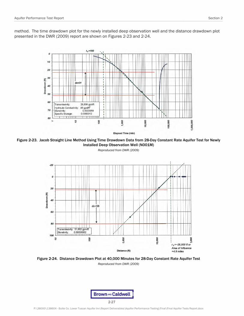
Aquifer Performance Test Report Section 2
2-27
P:\38000\138604 - Butte Co. Lower Tuscan Aquifer Inv\Report Deliverables\Aquifer Performance Testing\Final\Final Aquifer Tests Report.docx
method. The time drawdown plot for the newly installed deep observation well and the distance drawdown plot presented in the DWR (2009) report are shown on Figures 2-23 and 2-24.
Figure 2-23. Jacob Straight Line Method Using Time Drawdown Data from 28-Day Constant Rate Aquifer Test for Newly
Installed Deep Observation Well (N001M) Reproduced from DWR (2009)
Figure 2-24. Distance Drawdown Plot at 40,000 Minutes for 28-Day Constant Rate Aquifer Test
Reproduced from DWR (2009)

Section 2 Aquifer Performance Test Report
2-28
P:\38000\138604 - Butte Co. Lower Tuscan Aquifer Inv\Report Deliverables\Aquifer Performance Testing\Final\Final Aquifer Tests Report.docx
T values from these two methods ranged from 3,984 ft2/day to 4,259 ft2/day and S values ranged from 0.0004 to 0.00007. The T value calculated using the time drawdown data from the test production well was 4,941 ft2/day. Using an aquifer thickness of 480 feet, K values range from 8.3 ft/day to 10.3 ft/day consistent with the silty to clean sands logged during installation of the test production and observation well.
To assess the radius of influence from pumping the test production well, DWR (2009) used two methods: observing measured drawdown within observation wells; and, by estimating radius of influence from the distance drawdown plot shown on Figure 2-24. Using the first method, two wells screened within the pumped aquifer showed response to pumping of the test well, 01N001M (deep well in new observation well) and 15C002M (Figure 2-22). Well 15C002M is located approximately 2.2 miles from the test production well. The hydrograph from the next nearest observation well, 18C001M (4.8 miles from test production well), shows no observable response to pumping indicating that the influence of pumping becomes negligible between 2.2 miles and 4.8 miles. Using the second method illustrated on Figure 2-24, the estimated radius of influence is about 5 miles.
DWR (2009) also stated that the only well screened within aquifers shallower than the production well that showed a response to both pumping and recovery from the 28-day constant rate aquifer test was the intermediate deep well (01N002M) from the newly installed observation well. This well is screened approximately 100 feet above the pumped aquifer from 699 feet bgs to 709 feet bgs. DWR (2009) indicated that groundwater fluctuations within the remaining observation wells screened within shallower zones were due to seasonal variations or pumping of nearby irrigation or domestic wells screened within these zones.
2.3.4 Usability of Data
Although the software package AQTESOLV™ was available in 2007 when this aquifer test was conducted, DWR (2009) chose to analysis these tests using time drawdown graphs and the Jacob straight line method or distance drawdown plots. In AQTESOLV™ these methods are used to obtain preliminary estimates of T and S values for use in constraining the analysis of drawdown curves using other solutions. It should also be noted that the two methods used are only valid for portions of the drawdown curve that indicate radial flow in an infinite-acting confined aquifer. No analysis was conducted to confirm these assumptions such as could be done with AQTESOLV™. As discussed in Section 2.2.4, use of the derivative analysis provided in the AQTESOLV™ software package would also have provided more insight into an appropriate conceptual hydrogeologic model for the area. Based on the response to pumping from the intermediate deep well within the newly installed observation well, a solution that assumes a leaky confined aquifer such as Moench (1985) would provide more accurate values of T and S. However, the reported K values calculated from the reported T values are consistent with the silty sand and clean sands observed during drilling of the test and observation wells.
The DWR (2009) also shows that influence to pumping at a rate of 3,500 gpm within the deep aquifer was only observed at a distance of 2.2 miles from the test production well. No drawdown was observed in the next closest well screened in the pumped aquifer located approximately 4.8 miles from the test production well. The 28-day constant rate test also suggests that there is only hydraulic connection with the aquifer zone just above the deep aquifer zone. Other wells screened within shallower aquifer zones showed no response to pumping in the deep aquifer.
Based on review of the data presented in the above sections, the aquifer tests conducted for this project were performed in accordance with industry standards of the time and the data reported can be used to provide a better understanding of the Lower Tuscan Formation aquifer system’s hydraulic performance.
2.4 October 2009 Aquifer Test Report: Orland Site In 2009, Malcom Pirnie Inc. (Malcom Pirnie) performed an aquifer test using a test well constructed for the Crystal Geyser Water Company (Crystal Geyser). The stated objectives of the aquifer test were to:
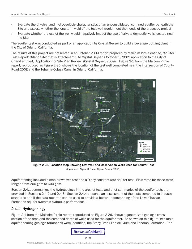
Aquifer Performance Test Report Section 2
2-29
P:\38000\138604 - Butte Co. Lower Tuscan Aquifer Inv\Report Deliverables\Aquifer Performance Testing\Final\Final Aquifer Tests Report.docx
Evaluate the physical and hydrogeologic characteristics of an unconsolidated, confined aquifer beneath the Site and assess whether the long-term yield of the test well would meet the needs of the proposed project
Evaluate whether the use of the well would negatively impact the use of private domestic wells located near the Site.
The aquifer test was conducted as part of an application by Crystal Geyser to build a beverage bottling plant in the City of Orland, California.
The results of this project are presented in an October 2009 report prepared by Malcolm Pirnie entitled, ‘Aquifer Test Report: Orland Site’ that is Attachment 5 to Crystal Geyser’s October 5, 2009 application to the City of Orland entitled, ‘Application for Site Plan Review’ (Crystal Geyser, 2009). Figure 3-1 from the Malcom Pirnie report, reproduced as Figure 2-25, shows the location of the test well completed near the intersection of County Road 200E and the Tehama-Colusa Canal in Orland, California.
Figure 2-25. Location Map Showing Test Well and Observation Wells Used for Aquifer Test
Reproduced Figure 3-1 from Crystal Geyser (2009)
Aquifer testing included a step-drawdown test and a 9-day constant rate aquifer test. Flow rates for these tests ranged from 200 gpm to 600 gpm.
Section 2.4.1 summarizes the hydrogeology in the area of tests and brief summaries of the aquifer tests are provided in Sections 2.4.2 and 2.4.3. Section 2.4.4 presents an assessment of the tests compared to industry standards and if the data reported can be used to provide a better understanding of the Lower Tuscan Formation aquifer system’s hydraulic performance.
2.4.1 Hydrogeology
Figure 2-1 from the Malcolm Pirnie report, reproduced as Figure 2-26, shows a generalized geologic cross section of the area and the screened depth of wells used for the aquifer test. As shown on this figure, two main aquifer-bearing geologic formations were identified, the Stony Creek Fan alluvium and Tehama Formation. The

Section 2 Aquifer Performance Test Report
2-30
P:\38000\138604 - Butte Co. Lower Tuscan Aquifer Inv\Report Deliverables\Aquifer Performance Testing\Final\Final Aquifer Tests Report.docx
Stony Creek Fan is identified as an unconfined aquifer. Underlying the Stony Creek Fan is the Tehama Formation where the upper 100 feet of this unit consists of a clay unit that acts as a confining layer between the Tehama upper aquifer system and the Stony Creek Fan aquifer system. Figure 2-26 also shows a 250 foot thick confining layer beneath the confined aquifer of the Tehama Formation.
Figure 2-26. Conceptual Profile of Subsurface Site Conditions, Crystal Geyser Facility
Reproduced Figure 2-1 from Crystal Geyser (2009)
Figure 2-26 also shows that the test well (PW-1) and observation wells (MW-1S and MW-2) installed for the project are completed within the confined aquifer system of the Tehama Formation. Other monitoring wells monitored during the aquifer test are completed within the Tehama Formation confined aquifer, upper confining unit of the Tehama Formation, and the Stony Creek Fan. As discussed in Section 2.4.3, MW-1 is a nested observation well with screen zones in the Tehama Formation confined aquifer and two deeper screened zones. The report or geologic well logs produced for the project do not indicate what geologic formations these wells are completed.
2.4.2 Step-Drawdown Aquifer Test
A step-drawdown aquifer test for the test well was conducted on July 1, 2009 consisting of four two hour steps pumping at rates of 200 gpm, 300 gpm, 400 gpm, and 500 gpm. A fifth 80 minute step was performed at a rate of 600 gpm. During the aquifer test water levels were measured in the test well using a pressure transducer programed to record water levels at intervals of 1-minute for the first 10 minutes of each step and then every 5 minutes thereafter. The purpose of the step-drawdown test was to select the appropriate pumping rate for the 9-day constant-discharge aquifer test.
The results of this aquifer test indicated that the test well could pump efficiently at any rate between 200 gpm and 600 gpm. Figure 2-27 shows the time-drawdown curve produced for step-drawdown aquifer test and includes the measured specific capacities. Specific capacities measured during the test ranged from 14 gpm/ft to 22 gpm/ft. No aquifer parameters such as T and K were estimated from the results of this test.
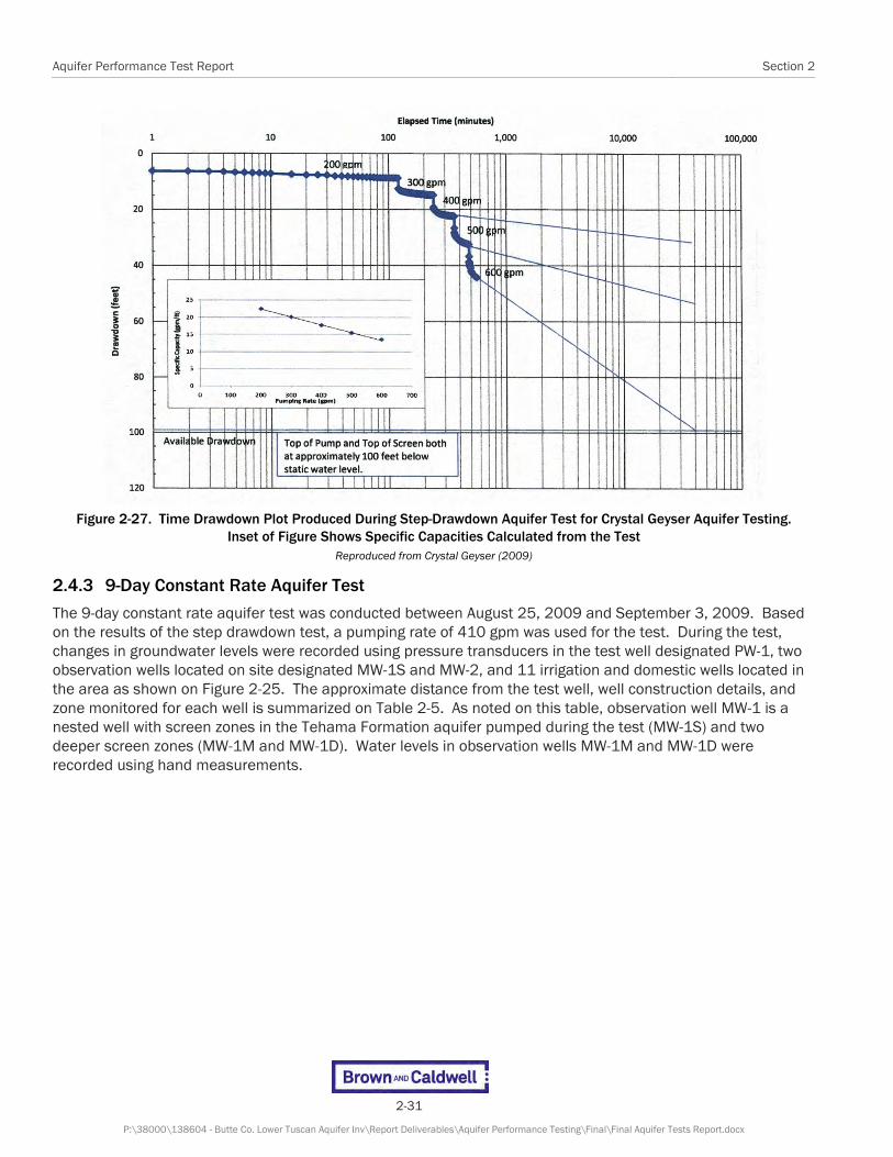
Aquifer Performance Test Report Section 2
2-31
P:\38000\138604 - Butte Co. Lower Tuscan Aquifer Inv\Report Deliverables\Aquifer Performance Testing\Final\Final Aquifer Tests Report.docx
Figure 2-27. Time Drawdown Plot Produced During Step-Drawdown Aquifer Test for Crystal Geyser Aquifer Testing.
Inset of Figure Shows Specific Capacities Calculated from the Test Reproduced from Crystal Geyser (2009)
2.4.3 9-Day Constant Rate Aquifer Test
The 9-day constant rate aquifer test was conducted between August 25, 2009 and September 3, 2009. Based on the results of the step drawdown test, a pumping rate of 410 gpm was used for the test. During the test, changes in groundwater levels were recorded using pressure transducers in the test well designated PW-1, two observation wells located on site designated MW-1S and MW-2, and 11 irrigation and domestic wells located in the area as shown on Figure 2-25. The approximate distance from the test well, well construction details, and zone monitored for each well is summarized on Table 2-5. As noted on this table, observation well MW-1 is a nested well with screen zones in the Tehama Formation aquifer pumped during the test (MW-1S) and two deeper screen zones (MW-1M and MW-1D). Water levels in observation wells MW-1M and MW-1D were recorded using hand measurements.
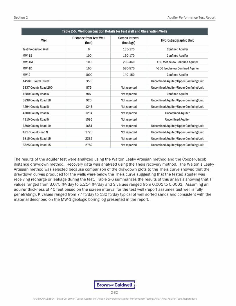
Section 2 Aquifer Performance Test Report
2-32
P:\38000\138604 - Butte Co. Lower Tuscan Aquifer Inv\Report Deliverables\Aquifer Performance Testing\Final\Final Aquifer Tests Report.docx
Table 2-5. Well Construction Details for Test Well and Observation Wells
Well Distance from Test Well
(feet) Screen Interval
(feet bgs) Hydrostratigraphic Unit
Test Production Well 0 135-175 Confined Aquifer
MW-1S 100 130-170 Confined Aquifer
MW-1M 100 290-340 >80 feet below Confined Aquifer
MW-1D 100 520-570 >300 feet below Confined Aquifer
MW-2 1000 140-150 Confined Aquifer
1450 E. South Street 353 Unconfined Aquifer/Upper Confining Unit
6837 County Road 200 875 Not reported Unconfined Aquifer/Upper Confining Unit
4280 County Road N 907 Not reported Confined Aquifer
6838 County Road 18 920 Not reported Unconfined Aquifer/Upper Confining Unit
4294 County Road N 1245 Not reported Unconfined Aquifer/Upper Confining Unit
4300 County Road N 1294 Not reported Unconfined Aquifer
4310 County Road N 1595 Not reported Unconfined Aquifer
6800 County Road 19 1681 Not reported Unconfined Aquifer/Upper Confining Unit
4317 Count Road N 1725 Not reported Unconfined Aquifer/Upper Confining Unit
6815 County Road 15 2332 Not reported Unconfined Aquifer/Upper Confining Unit
6825 County Road 15 2782 Not reported Unconfined Aquifer/Upper Confining Unit
The results of the aquifer test were analyzed using the Walton Leaky Artesian method and the Cooper-Jacob distance drawdown method. Recovery data was analyzed using the Theis recovery method. The Walton’s Leaky Artesian method was selected because comparison of the drawdown plots to the Theis curve showed that the drawdown curves produced for the wells were below the Theis curve suggesting that the tested aquifer was receiving recharge or leakage during the test. Table 2-6 summarizes the results of this analysis showing that T values ranged from 3,075 ft2/day to 5,214 ft2/day and S values ranged from 0.001 to 0.0001. Assuming an aquifer thickness of 40 feet based on the screen interval for the test well (report assumes test well is fully penetrating), K values ranged from 77 ft/day to 130 ft/day typical of well sorted sands and consistent with the material described on the MW-1 geologic boring log presented in the report.

Aquifer Performance Test Report Section 2
2-33
P:\38000\138604 - Butte Co. Lower Tuscan Aquifer Inv\Report Deliverables\Aquifer Performance Testing\Final\Final Aquifer Tests Report.docx
Table 2-6. Summary of Aquifer Test Analysis during 9-day Constant Rate Aquifer Test
Well I.D./Analysis Method T
(ft2/day) S
(unitless)
Walton’s Leaky Artesian
MW-1S 3,075 0.0006
MW-2 4,545 0.0001
Cooper-Jacob Distance Drawdown
t = 2,000 minutes 5,214 0.001
t = 7,300 minutes 5,214 0.0006
Theis Recovery
PW-1 3,877 NA
MW-1S 3,743 NA
MW-2 4,278 NA
The Malcom Pirnie report also states that based on the hydrographs produced for the 11 observation wells, pumping of the test well in the confined aquifer of the Tehama Formation did not affect wells screened within the upper confining layer of the Tehama Formation or the unconfined aquifer within the Stony Creek Fan. Although the report indicates that water levels were recorded in the deeper screened intervals of observation well MW-1, this data was not presented in the report. The report also does not indicate the geologic formation these wells are completed in.
2.4.4 Usability of Data
Based on review of the data presented in the above sections, the aquifer tests conducted for this project were performed in accordance with industry standards. However, neither the pumping well nor the observation wells used for the test were completed within the Tuscan Formation. As such, the data reported for this test is not usable for providing a better understanding of the Lower Tuscan Formation aquifer system’s hydraulic performance.


3-1
P:\38000\138604 - Butte Co. Lower Tuscan Aquifer Inv\Report Deliverables\Aquifer Performance Testing\Final\Final Aquifer Tests Report.docx
Section 3
Methods and Procedures for LTA Aquifer Test and Analysis Three separate aquifer performance tests were conducted as part of the LTA project using existing production wells connected to irrigation distribution systems (Figure 1-1). The water extracted was used as part of existing irrigation practices and distributed according to normal operating conditions at each location. Prior to use, each location was reviewed and cleared as part of the Initial Study for the project (Butte County, 2010). As discussed in the introduction, the purpose of the aquifer tests is to monitor the LTA’s response to pumping, assess interaction with other aquifers, and to use the data to estimate aquifer parameters.
A summary of the methods and procedures used to conduct each of the tests is presented in the following sections. The aquifer tests were performed in accordance with American Society for Testing and Materials Method D 4050 as modified in the Technical Memorandum Number 3 prepared for the project (Brown and Caldwell, 2011). As stated in Section 1, the three aquifer tests are referred to as the Hackett Property (north), M&T Ranch (central), and Esquon Ranch (south) aquifer tests.
3.1 Hackett Property Aquifer Test Figure 3-1 shows a close-up of the aquifer test area conducted on the Hackett Property including the location of the pumping well, primary observation wells, and other known irrigation supply wells. For this aquifer test, the primary observation well was installed as part of the overall LTA project and is designated MW-HP-1. Observation well MW-HP-1 is a nested well consisting of three separate screen intervals within the same borehole. A detailed discussion of the installation of this well including lithologic information obtained during drilling is presented in the Field Investigation Report (Brown and Caldwell, 2012). The pumping well (Figure 3-1) used for this aquifer test is designated PW-HP-1. Well construction details for the pumping well and primary observation wells are provided on Table 3-1.

Section 3 Aquifer Performance Test Report
3-2
P:\38000\138604 - Butte Co. Lower Tuscan Aquifer Inv\Report Deliverables\Aquifer Performance Testing\Final\Final Aquifer Tests Report.docx
Figure 3-1. Hackett Property Aquifer Test Location Illustrating Monitoring Well and Pumping Well Locations
Table 3-1. Well Construction Details for Hackett Property Aquifer Test
Well I.D. Latitude Longitude Distance From Pumping Well
(Feet)
Screen Interval
(Feet bgs)
Filter Pack Interval
(Feet bgs)
Well Diameter (inches)
Borehole Diameter (inches)
PW-HP-1 39.8779464 -121.4408264 0 309-344 309-344 10 12
MW-HP-1
Shallow Screen 39.87821558 -121.9570981 148 70-100 60-115 2.5 12
Intermediate Screen 39.87821558 -121.9570981 148 320-340 309-351 2.5 12
Deep Screen 39.87821558 -121.9570981 148 510-540 499-556 2.5 12

Aquifer Performance Test Report Section 3
3-3
P:\38000\138604 - Butte Co. Lower Tuscan Aquifer Inv\Report Deliverables\Aquifer Performance Testing\Final\Final Aquifer Tests Report.docx
Prior to startup of the aquifer test, the pumping well and observation wells were outfitted with pressure transducers to record water level changes. Pressure transducers used for the aquifer tests were the In-Situ Level Troll 500 vented transducers (Figure 3-2). The vented transducers self-correct for barometric changes eliminating the need for a barometer during the tests. The property owner also insured that irrigation wells PW-HP-2 through PW-HP-4 (Figure 3-1) were not operated during the aquifer test so no monitoring of these wells were included during the aquifer test. Well PW-HP-5 shown on Figure 3-1 is a supply well for a nearby gravel mine. It is believed that this well did operate during the aquifer test based on the response of the deep observation well within MW-HP-1 as discussed in Section 4.1.
Figure 3-2. Picture of typical pressure transducer used for LTA aquifer tests. Length of cable will vary.
Immediately before pumping began, static water levels were recorded for the pumping well and the primary observation wells using a hand held electric well sounder. Table 3-2 summarizes the results of these measurements. The pressure transducers were then set to record water levels every one second for a minimum of 1-hour after startup of the test. The pressure transducers were then reprogramed to record water levels every minute if there was a water level change greater than 0.1 feet, otherwise water levels were recorded every 10-minutes.
Table 3-2. Summary of Static Water Level Measurements
Well I.D. Pressure Transducer Reading
(feet of water above) Depth to Water
(feet below measure point) Measuring Point Elevation
(feet above mean sea level)
PW-HP-1 69.325 39.63 217.91
MW-HP-1
Shallow Screen 40.564 34.64 219.59
Intermediate Screen 58.890 41.72 219.59
Deep Screen 23.764 44.15 219.59
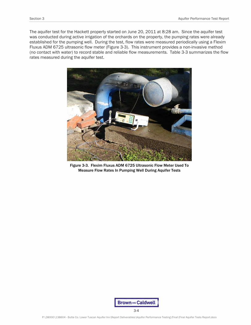
Section 3 Aquifer Performance Test Report
3-4
P:\38000\138604 - Butte Co. Lower Tuscan Aquifer Inv\Report Deliverables\Aquifer Performance Testing\Final\Final Aquifer Tests Report.docx
The aquifer test for the Hackett property started on June 20, 2011 at 8:28 am. Since the aquifer test was conducted during active irrigation of the orchards on the property, the pumping rates were already established for the pumping well. During the test, flow rates were measured periodically using a Flexim Fluxus ADM 6725 ultrasonic flow meter (Figure 3-3). This instrument provides a non-invasive method (no contact with water) to record stable and reliable flow measurements. Table 3-3 summarizes the flow rates measured during the aquifer test.
Figure 3-3. Flexim Fluxus ADM 6725 Ultrasonic Flow Meter Used To
Measure Flow Rates In Pumping Well During Aquifer Tests

Aquifer Performance Test Report Section 3
3-5
P:\38000\138604 - Butte Co. Lower Tuscan Aquifer Inv\Report Deliverables\Aquifer Performance Testing\Final\Final Aquifer Tests Report.docx
Table 3-3. Pumping Rates Recorded During Hackett Property Aquifer Test
Time From Start (Minutes)
Pumping Rate (gpm)
0 834
72 813
182 790
538 780
1396 750
1397 880
1399 970
1406 840
1718 808
2797 900
2861 960
3303 925
4224 953
4230 1202
4237 1000
4642 953
5664 785
5982 730
6211 0
During the test, water levels were also periodically measured manually using an electronic well sounder. Table 3-4 summarizes these measurements.

Section 3 Aquifer Performance Test Report
3-6
P:\38000\138604 - Butte Co. Lower Tuscan Aquifer Inv\Report Deliverables\Aquifer Performance Testing\Final\Final Aquifer Tests Report.docx
Table 3-4. Hand Water Level Measurements Collected During Hackett Property Aquifer Test
Well I.D. Date Time
(24 hour) Depth to Water
(feet below measuring point)1
PW-HP-1 6/20/11
1026
1210
77.05
78.0
6/24/11 1649 44.45
MW-HP-1
Shallow Screen
6/20/11
1023
1206
1702
35.97
36.12
36.21
6/21/11 0818 36.54
6/22/11 0815 36.91
6/23/11 0800 37.19
6/24/11 1643 36.12
Intermediate Screen
6/20/11
1022
1205
1701
63.52
64.81
65.17
6/21/11 0817 65.84
6/22/11 0814 69.55
6/23/11 0758 71.66
6/24/11 1642 47.30
Deep Screen
6/20/11
1020
1203
1700
43.93
43.94
43.92
6/21/11 0815 43.41
6/22/11 0813 42.94
6/23/11 0756 43.03
6/24/11 1641 44.92
1. See Table 3-2
The aquifer test stopped on June 24, 2011 at 4:00 pm for a total pumping time of approximately 103.5 hours. Immediately prior to shut-off, the pressure transducers were reprogramed to record water levels every 5-seconds. After a minimum of 1-hour after shutoff, the pressure transducers were reprogramed to record water levels during recovery if there was a water level change greater than 0.1 feet, otherwise water levels were recorded every 10-minutes. Recovery was recorded for over one month and the pressure transducers were downloaded on August 16, 2011.
3.2 M&T Ranch Aquifer Test Figure 3-4 shows a close-up of the aquifer test area conducted on the M&T Ranch including the location of the pumping well, primary observation wells, and other known irrigation supply wells. For this aquifer test, the primary observation well was installed as part of the overall LTA project and is designated MW-MT-1 (State Well Number (SWN) 23N01W03H002M). Observation well MW-MT-1 is a nested well

Aquifer Performance Test Report Section 3
3-7
P:\38000\138604 - Butte Co. Lower Tuscan Aquifer Inv\Report Deliverables\Aquifer Performance Testing\Final\Final Aquifer Tests Report.docx
consisting of three separate screen intervals within the same borehole. A detailed discussion of the installation of this well including lithologic information obtained during drilling is presented in the Field Investigation Report (Brown and Caldwell, 2012b). The pumping well (Figure 3-4) used for this aquifer test is designated PW-MT-1. Irrigation wells PW-MT-2 and PW-MT-3 are wells that operated during the aquifer test. As discussed in Section 2.2, well PW-MT-4 is the test production well used for a 1996 aquifer test conducted by DWR (1996). Well construction details for the pumping well and primary observation wells are provided on Table 3-5.
Figure 3-4. M&T Ranch Aquifer Test Location Illustrating Monitoring Well and Pumping Well Locations
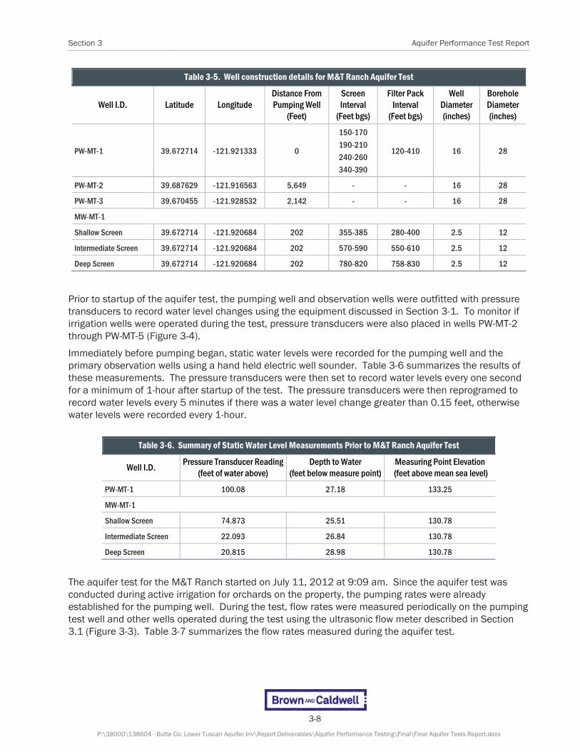
Section 3 Aquifer Performance Test Report
3-8
P:\38000\138604 - Butte Co. Lower Tuscan Aquifer Inv\Report Deliverables\Aquifer Performance Testing\Final\Final Aquifer Tests Report.docx
Table 3-5. Well construction details for M&T Ranch Aquifer Test
Well I.D. Latitude Longitude Distance From Pumping Well
(Feet)
Screen Interval
(Feet bgs)
Filter Pack Interval
(Feet bgs)
Well Diameter (inches)
Borehole Diameter (inches)
PW-MT-1 39.672714 -121.921333 0
150-170
190-210
240-260
340-390
120-410 16 28
PW-MT-2 39.687629 -121.916563 5,649 - - 16 28
PW-MT-3 39.670455 -121.928532 2,142 - - 16 28
MW-MT-1
Shallow Screen 39.672714 -121.920684 202 355-385 280-400 2.5 12
Intermediate Screen 39.672714 -121.920684 202 570-590 550-610 2.5 12
Deep Screen 39.672714 -121.920684 202 780-820 758-830 2.5 12
Prior to startup of the aquifer test, the pumping well and observation wells were outfitted with pressure transducers to record water level changes using the equipment discussed in Section 3-1. To monitor if irrigation wells were operated during the test, pressure transducers were also placed in wells PW-MT-2 through PW-MT-5 (Figure 3-4).
Immediately before pumping began, static water levels were recorded for the pumping well and the primary observation wells using a hand held electric well sounder. Table 3-6 summarizes the results of these measurements. The pressure transducers were then set to record water levels every one second for a minimum of 1-hour after startup of the test. The pressure transducers were then reprogramed to record water levels every 5 minutes if there was a water level change greater than 0.15 feet, otherwise water levels were recorded every 1-hour.
Table 3-6. Summary of Static Water Level Measurements Prior to M&T Ranch Aquifer Test
Well I.D. Pressure Transducer Reading
(feet of water above) Depth to Water
(feet below measure point) Measuring Point Elevation
(feet above mean sea level)
PW-MT-1 100.08 27.18 133.25
MW-MT-1
Shallow Screen 74.873 25.51 130.78
Intermediate Screen 22.093 26.84 130.78
Deep Screen 20.815 28.98 130.78
The aquifer test for the M&T Ranch started on July 11, 2012 at 9:09 am. Since the aquifer test was conducted during active irrigation for orchards on the property, the pumping rates were already established for the pumping well. During the test, flow rates were measured periodically on the pumping test well and other wells operated during the test using the ultrasonic flow meter described in Section 3.1 (Figure 3-3). Table 3-7 summarizes the flow rates measured during the aquifer test.

Aquifer Performance Test Report Section 3
3-9
P:\38000\138604 - Butte Co. Lower Tuscan Aquifer Inv\Report Deliverables\Aquifer Performance Testing\Final\Final Aquifer Tests Report.docx
Table 3-7. Pumping Rates Recorded During M&T Ranch Aquifer Test
PW-MT-1 PW-MT-3 PW-MT-2
Time From Start (minutes)
Pumping Rate (gpm)
Time From Start (minutes)
Pumping Rate (gpm)
Time From Start (minutes)
Pumping Rate (gpm)
0 1850 0 0 0 0
5 1765 1900 1690 659 1589
14 1748 2896 1626 1468 1594
28 1743 3193 1622 1874 0
36 1750 3244 1602
114 1775 4492 0
685 1700
1495 1615
2025 1772
2905 1620
3335 1770
3358 1768
6336 0
The aquifer test ended on July 15, 2012 at 6:44 pm for a total pumping time of approximately 105 hours. Recovery was recorded for over 14 hours and the pressure transducers were downloaded on July 16, 2012.
3.3 Esquon Ranch Aquifer Test Figure 3-5 shows a close-up of the aquifer test area conducted on the Esquon Ranch including the location of the pumping wells, primary observation wells, and other known irrigation supply wells. For this aquifer test, the primary observation well was an existing observation well installed by DWR and is designated MW-ESQ-1 (SWN 21N02E26E03-06M). Observation well MW-ESQ-1 is a nested well consisting of four separate screen intervals within the same borehole. A second observation well installed by DWR was also monitored for this test designated MW-ESQ-2 (SWN 20N02E09M) (Figure 3-5). The geologic well logs for these two wells are presented in Appendix C. Two pumping wells were used for this aquifer test designated PW-ESQ-39 and PW-ESQ-40 (Figure 3-5). Other Irrigation wells that operated during the aquifer test and affected drawdown curves included PW-ESQ-12, PW-ESQ-13, PW-ESQ-16, and PW-ESQ-22. Well construction details for the pumping well and primary observation wells are provided on Table 3-8.

Section 3 Aquifer Performance Test Report
3-10
P:\38000\138604 - Butte Co. Lower Tuscan Aquifer Inv\Report Deliverables\Aquifer Performance Testing\Final\Final Aquifer Tests Report.docx
Figure 3-5. Esquon Ranch Aquifer Test Location Illustrating Monitoring Well and Pumping Well Locations
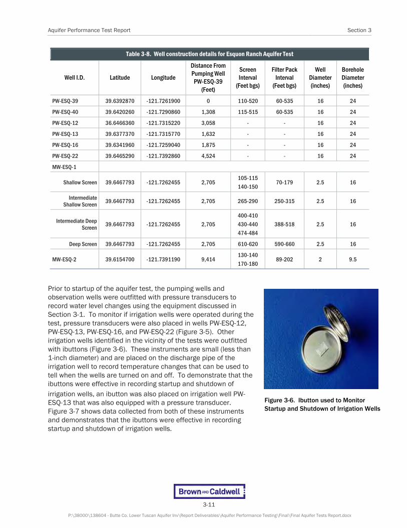
Aquifer Performance Test Report Section 3
3-11
P:\38000\138604 - Butte Co. Lower Tuscan Aquifer Inv\Report Deliverables\Aquifer Performance Testing\Final\Final Aquifer Tests Report.docx
Table 3-8. Well construction details for Esquon Ranch Aquifer Test
Well I.D. Latitude Longitude
Distance From Pumping Well PW-ESQ-39
(Feet)
Screen Interval
(Feet bgs)
Filter Pack Interval
(Feet bgs)
Well Diameter (inches)
Borehole Diameter (inches)
PW-ESQ-39 39.6392870 -121.7261900 0 110-520 60-535 16 24
PW-ESQ-40 39.6420260 -121.7290860 1,308 115-515 60-535 16 24
PW-ESQ-12 36.6466360 -121.7315220 3,058 - - 16 24
PW-ESQ-13 39.6377370 -121.7315770 1,632 - - 16 24
PW-ESQ-16 39.6341960 -121.7259040 1,875 - - 16 24
PW-ESQ-22 39.6465290 -121.7392860 4,524 - - 16 24
MW-ESQ-1
Shallow Screen 39.6467793 -121.7262455 2,705 105-115
140-150 70-179 2.5 16
Intermediate Shallow Screen
39.6467793 -121.7262455 2,705 265-290 250-315 2.5 16
Intermediate Deep Screen
39.6467793 -121.7262455 2,705
400-410
430-440
474-484
388-518 2.5 16
Deep Screen 39.6467793 -121.7262455 2,705 610-620 590-660 2.5 16
MW-ESQ-2 39.6154700 -121.7391190 9,414 130-140
170-180 89-202 2 9.5
Prior to startup of the aquifer test, the pumping wells and observation wells were outfitted with pressure transducers to record water level changes using the equipment discussed in Section 3-1. To monitor if irrigation wells were operated during the test, pressure transducers were also placed in wells PW-ESQ-12, PW-ESQ-13, PW-ESQ-16, and PW-ESQ-22 (Figure 3-5). Other irrigation wells identified in the vicinity of the tests were outfitted with ibuttons (Figure 3-6). These instruments are small (less than 1-inch diameter) and are placed on the discharge pipe of the irrigation well to record temperature changes that can be used to tell when the wells are turned on and off. To demonstrate that the ibuttons were effective in recording startup and shutdown of irrigation wells, an ibutton was also placed on irrigation well PW-ESQ-13 that was also equipped with a pressure transducer. Figure 3-7 shows data collected from both of these instruments and demonstrates that the ibuttons were effective in recording startup and shutdown of irrigation wells.
Figure 3-6. Ibutton used to Monitor Startup and Shutdown of Irrigation Wells

Section 3 Aquifer Performance Test Report
3-12
P:\38000\138604 - Butte Co. Lower Tuscan Aquifer Inv\Report Deliverables\Aquifer Performance Testing\Final\Final Aquifer Tests Report.docx
Figure 3-7. Plot of drawdown data recorded by pressure transducer and temperature data recorded by ibutton
over same time period at irrigation well PW-ESQ-13. When irrigation well is turned on, temperature data becomes more constant reflecting temperature of water within discharge pipe. When irrigation well turns off,
temperature data reflects fluctuations between night time and day time.
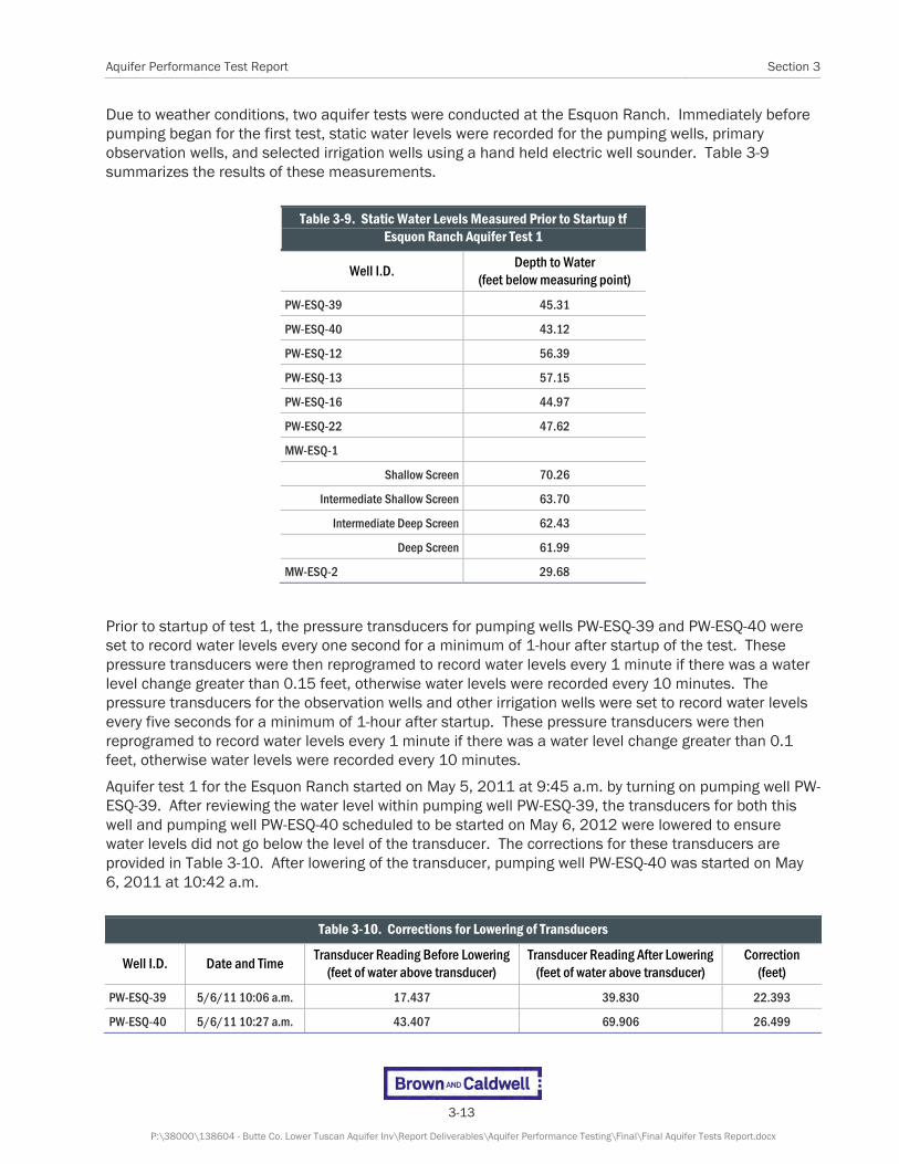
Aquifer Performance Test Report Section 3
3-13
P:\38000\138604 - Butte Co. Lower Tuscan Aquifer Inv\Report Deliverables\Aquifer Performance Testing\Final\Final Aquifer Tests Report.docx
Due to weather conditions, two aquifer tests were conducted at the Esquon Ranch. Immediately before pumping began for the first test, static water levels were recorded for the pumping wells, primary observation wells, and selected irrigation wells using a hand held electric well sounder. Table 3-9 summarizes the results of these measurements.
Table 3-9. Static Water Levels Measured Prior to Startup tf Esquon Ranch Aquifer Test 1
Well I.D. Depth to Water
(feet below measuring point)
PW-ESQ-39 45.31
PW-ESQ-40 43.12
PW-ESQ-12 56.39
PW-ESQ-13 57.15
PW-ESQ-16 44.97
PW-ESQ-22 47.62
MW-ESQ-1
Shallow Screen 70.26
Intermediate Shallow Screen 63.70
Intermediate Deep Screen 62.43
Deep Screen 61.99
MW-ESQ-2 29.68
Prior to startup of test 1, the pressure transducers for pumping wells PW-ESQ-39 and PW-ESQ-40 were set to record water levels every one second for a minimum of 1-hour after startup of the test. These pressure transducers were then reprogramed to record water levels every 1 minute if there was a water level change greater than 0.15 feet, otherwise water levels were recorded every 10 minutes. The pressure transducers for the observation wells and other irrigation wells were set to record water levels every five seconds for a minimum of 1-hour after startup. These pressure transducers were then reprogramed to record water levels every 1 minute if there was a water level change greater than 0.1 feet, otherwise water levels were recorded every 10 minutes.
Aquifer test 1 for the Esquon Ranch started on May 5, 2011 at 9:45 a.m. by turning on pumping well PW-ESQ-39. After reviewing the water level within pumping well PW-ESQ-39, the transducers for both this well and pumping well PW-ESQ-40 scheduled to be started on May 6, 2012 were lowered to ensure water levels did not go below the level of the transducer. The corrections for these transducers are provided in Table 3-10. After lowering of the transducer, pumping well PW-ESQ-40 was started on May 6, 2011 at 10:42 a.m.
Table 3-10. Corrections for Lowering of Transducers
Well I.D. Date and Time Transducer Reading Before Lowering
(feet of water above transducer) Transducer Reading After Lowering
(feet of water above transducer) Correction
(feet)
PW-ESQ-39 5/6/11 10:06 a.m. 17.437 39.830 22.393
PW-ESQ-40 5/6/11 10:27 a.m. 43.407 69.906 26.499
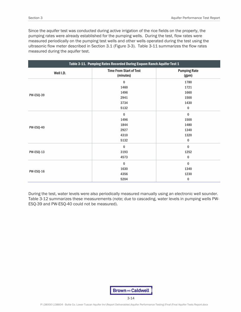
Section 3 Aquifer Performance Test Report
3-14
P:\38000\138604 - Butte Co. Lower Tuscan Aquifer Inv\Report Deliverables\Aquifer Performance Testing\Final\Final Aquifer Tests Report.docx
Since the aquifer test was conducted during active irrigation of the rice fields on the property, the pumping rates were already established for the pumping wells. During the test, flow rates were measured periodically on the pumping test wells and other wells operated during the test using the ultrasonic flow meter described in Section 3.1 (Figure 3-3). Table 3-11 summarizes the flow rates measured during the aquifer test.
Table 3-11. Pumping Rates Recorded During Esquon Ranch Aquifer Test 1
Well I.D. Time From Start of Test
(minutes) Pumping Rate
(gpm)
PW-ESQ-39
0
1460
1496
2941
3734
5132
1780
1721
1660
1500
1430
0
PW-ESQ-40
0
1496
1844
2927
4310
5132
0
1500
1480
1340
1320
0
PW-ESQ-13
0
3193
4573
0
1252
0
PW-ESQ-16
0
1630
4356
5204
0
1340
1230
0
During the test, water levels were also periodically measured manually using an electronic well sounder. Table 3-12 summarizes these measurements (note; due to cascading, water levels in pumping wells PW-ESQ-39 and PW-ESQ-40 could not be measured).

Aquifer Performance Test Report Section 3
3-15
P:\38000\138604 - Butte Co. Lower Tuscan Aquifer Inv\Report Deliverables\Aquifer Performance Testing\Final\Final Aquifer Tests Report.docx
Table 3-12. Hand Water Level Measurements Collected During Esquon Ranch Aquifer Test 1
Well I.D. Date Time
(24 hour) Depth to Water
(feet below measuring point)
MW-ESQ-1
Shallow Screen 5/7/11 0823 70.38
5/8/11 0725 70.47
Intermediate Shallow Screen 5/7/11 0825 74.19
5/8/11 0727 75.75
Intermediate Deep Screen 5/7/11 0827 70.68
5/8/11 0728 72.48
Deep Screen 5/7/11 0828 63.61
5/8/11 0729 65.43
MW-ESQ-2 5/7/11 0946 31.34
5/8/11 0909 31.37
PW-ESQ-12 5/7/11 0903 57.97
5/8/11 0845 Cascading – could not measure
PW-ESQ-16 5/7/11 1005 78.09
5/8/11 1022 Cascading – could not measure
PW-ESQ-22
5/7/11 0909 49.72
5/8/11 0852 Well pumping. Water level below
transducer
On May 8, 2011 at approximately 11:00 p.m., a lighting strike hit a transformer turning off all of the pumping wells for a total pumping time of about 85.5 hours. After allowing a minimum of 48 hours for water levels to recover, the test was restarted on May 13, 2011 at 08:15 a.m. For this test, pumping wells PW-ESQ-39 and PW-ESQ-40 were started simultaneously. After startup of this test, it was noted that the clock within the pressure transducers placed in observation well MW-ESQ-1 were not synchronized with the computer clock used to synchronize the other transducers. Table 3-13 provides the corrections for times recorded on these transducers.
Table 3-13. Time Corrections MW-ESQ-1 Transducers During Esquon Ranch Aquifer Test 2
Screen Zone Date Transducer Time Computer Time Correction
(minutes:seconds)
Shallow 5/13/11 10:32:07 10:20:19 -12:12
Intermediate Shallow 5/13/11 10:37:29 10:37:15 -00:14
Intermediate Deep 5/13/11 10:30:40 10:19:57 -11:43
Deep 5/13/11 10:34:26 10:22:54 -12:32

Section 3 Aquifer Performance Test Report
3-16
P:\38000\138604 - Butte Co. Lower Tuscan Aquifer Inv\Report Deliverables\Aquifer Performance Testing\Final\Final Aquifer Tests Report.docx
Table 3-14 summarizes the pumping rates recorded during this second aquifer test.
Table 3-14. Pumping Rates Recorded During Esquon Ranch Aquifer Test 2
Well I.D. Time From Start of Test
(minutes) Pumping Rate
(gpm)
PW-ESQ-39
0
7379
9024
11687
1750
1390
1395
0
PW-ESQ-40
0
7392
9050
11687
1500
1165
1180
0
PW-ESQ-12
0
5966
7244
8951
10364
0
1203
0
1390
0
PW-ESQ-13
0
394
8942
10482
10493
0
1252
1195
1178
0
PW-ESQ-16
0
5897
9013
11687
1230
1270
1260
0
PW-ESQ-22
0
2988
5966
6156
9584
11484
0
1614
1246
0
1246
0
Table 3-15 summarizes hand water level measurements collected from observation well MW-ESQ-1 during aquifer test 2.

Aquifer Performance Test Report Section 3
3-17
P:\38000\138604 - Butte Co. Lower Tuscan Aquifer Inv\Report Deliverables\Aquifer Performance Testing\Final\Final Aquifer Tests Report.docx
Table 3-15. Hand Water Level Measurements for MW-ESQ-1 Collected During Esquon Ranch Aquifer Test 2
Well I.D. Date Time
(24 hour) Depth to Water
(feet below measuring point)
Shallow Screen
5/17/11 0921 71.54
5/18/11 1248 71.84
5/19/11 0839 72.13
Intermediate Shallow Screen
5/17/11 0922 80.76
5/18/11 1249 80.12
5/19/11 0841 80.17
Intermediate Deep Screen
5/17/11 0924 77.64
5/18/11 1251 77.32
5/19/11 0844 77.28
Deep Screen
5/17/11 0925 71.15
5/18/11 1252 72.49
5/19/11 0845 73.05
On May 21, 2011 at 11:03 a.m., another lighting strike hit a transformer turning off all of the pumping wells for a total pumping time of about 195 hours. Recovery was recorded for over one month and the pressure transducers were downloaded on June 15, 2011.
3.4 Groundwater Sampling Groundwater samples were collected from each of the pumping wells used for the aquifer tests during the LTA project after a minimum of 24 hours after startup of the aquifer tests. A summary of this sampling including wells sampled and date collected is provided in Table 3-16.
Table 3-16. Summary of Groundwater Sample Collection
Well I.D. Date Collected Days after Start of Aquifer
Test
PW-ESQ-39 5/20/11 7
PW-ESQ-40 5/20/11 7
PW-MT-1 7/12/12 1
PW-MT-2 7/12/12 1
PW-HP-1 6/24/11 4
For the M&T Ranch aquifer test an additional groundwater sample was collected from another irrigation well that was operating during the performance of the test (PW-MT-2; Figure 3-4). Groundwater samples were collected by filling the containers supplied by the analytical laboratory directly from sampling ports attached to each of the discharge lines associated with the pumping wells. For cation analysis, water was field filter with a 0.45 micrometer inline filter. Immediately after sampling field parameters were recorded including pH, specific conductivity, and temperature. The field meter was inoperative during

Section 3 Aquifer Performance Test Report
3-18
P:\38000\138604 - Butte Co. Lower Tuscan Aquifer Inv\Report Deliverables\Aquifer Performance Testing\Final\Final Aquifer Tests Report.docx
the Hackett Property sampling event, as such; these parameters were not recorded for this groundwater sample.
Samples were submitted under chain of custody documentation to California Laboratory Services of Rancho Cordova, California for analysis of cations, anions, and general parameters and to Zymax Forensics of Escondido, California for analysis of oxygen and deuterium isotopes. Copies of the chain-of-custody forms and the analytical laboratory reports are presented in Appendix D.

4-1
P:\38000\138604 - Butte Co. Lower Tuscan Aquifer Inv\Report Deliverables\Aquifer Performance Testing\Final\Final Aquifer Tests Report.docx
Section 4
Results and Analysis of LTA Aquifer Tests Analysis of the LTA aquifer tests discussed in Section 3 followed a stepwise process focused on assessing both the characteristics and interactions of the aquifers and calculation of aquifer properties. The first step involved developing a conceptual hydrogeologic model using the lithologic data obtained during the drilling of monitoring wells for the project. A clear understanding of the hydrogeology including identification of geologic formation boundaries is critical to an accurate interpretation of aquifer test data. For the LTA project, the selected drilling method was based on the ability to provide depth discrete lithologic samples and strict protocols were developed to identify geologic units from drill cuttings based on the methods of Blair and others (1991) and presented in Technical Memorandum Number 1 (Brown and Caldwell, 2010). This detailed geologic information also allowed the placement of screen intervals within specific hydrogeologic zones that provided detailed data on individual hydrogeologic zones and interactions between aquifers during the aquifer tests. Having accurate lithologic data from known well completions also assists in the interpretation of driller’s logs produced during the installation of pumping wells used for the aquifer tests.
After development of the conceptual hydrogeologic model, drawdown curves from the observation and pumping wells were visually assessed prior to calculating aquifer parameters. To calculate aquifer parameters, drawdown curves developed from the aquifer test from pumping wells and observation wells are compared to type curves developed from mathematical solutions of the flow equation. Type curves developed from these methods are based on specific assumptions about the characteristics of the aquifer. For example, the classic Theis solution assumes that the aquifer has infinite areal extent and is homogeneous, isotropic, and of uniform thickness. If the actual aquifer characteristics are distinctly different from these assumptions, then the drawdown curves observed for wells during the test will not match the type curves and aquifer parameters cannot be calculated. However, departures from the type curves can provide important qualitative interpretations of the aquifer characteristics that are essential for construction of future groundwater models developed for the basin as a management tool, design of subsequent aquifer tests, and design and construction of future irrigation and groundwater supply wells.
After determining if the drawdown curves adequately addressed the assumptions for type curve analysis, aquifer parameters were calculated using the software package AQTESOLV™. This software package also includes several diagnostic tools to assess flow regimes to select the appropriate type curve solution for the data including derivative analyses that are useful for detecting deviations in the rate of displacement change. As discussed in the AQTESOLV™ Version 4.5 User Guide (Duffield, 2007), this technique was introduced by Bourdet and others (1983, 1989) to the petroleum industry as a valuable diagnostic tool that can help identify aquifer responses such as aquifer boundaries, leakage, and delayed gravity response. Spane and Wurster (1993) furthered the use of these analyses for the groundwater industry.
This section presents an overview of the hydrostratigraphy within the project boundaries followed by summaries of the development of the site conceptual hydrogeologic model, visual assessment of drawdown curves, and analysis using the AQTESOLV™ software package at the three aquifer test sites discussed in Section 3. A detailed presentation of the quantitative curve matching performed using the AQTESOLV™ software package for each of the tests is presented in Appendix E. The discussion

Section 4 Aquifer Performance Test Report
4-2
P:\38000\138604 - Butte Co. Lower Tuscan Aquifer Inv\Report Deliverables\Aquifer Performance Testing\Final\Final Aquifer Tests Report.docx
presented in Appendix E for each aquifer test provides a summary of the assumptions develop for each of the analytical solutions used and an assessment of how actual conditions meet these assumptions. The complete set of drawdown data recorded by the transducers for each test is included within the project geodatabase. AQTESOLV also provides a diagnostic statistical report for each of the curve matching solutions. Copies of these reports are provided in Appendix F.
4.1 Hydrostratigraphy The Tuscan Formation includes a sequence of variably cemented, interbedded clay, sand, and gravel. This formation consists predominantly of purple volcanic debris flow deposits and interbedded waterlain fluvial deposits rich in volcanic detritus, but in many areas containing crystalline basement-derived clasts and rare tuff beds. The reported occurrence of both channel-lain, clast supported, pebble- and cobble-gravel facies and interbedded volcanic-rich debris-flow facies in this formation suggests that debris flows related to volcanic events episodically choked the ancestral stream/river systems of the area (Blair and others, 1991).
Helley and Hardwood (1985) divided the Tuscan Formation into four hydrostratigraphic units, labeled from deepest to shallowest, A through D. Units A and B together define the LTA, the subject of this study, and units C and D define the Upper Tuscan Aquifer. The approximate extent of the LTA within the project boundaries is shown on Figure 1-1. Helley and Hardwood (1985) also identified several tuffaceous units that were used to separate the hydrostratigraphic units that included the Tuff of Hogback Road (separates Unit D from Unit C), Ishi Tuff Member (separates Unit C from Unit B), and the Nomlaki Tuff Member (base of Unit A).
Overlying the Tuscan Formation are numerous Quaternary deposits (Qd). For the LTA project this unit was designated as Qd. This broader definition is employed because the numerous Quaternary formations others have proposed are based on geomorphic or buried-soil information rather than on criteria by which formal formations are distinguished. More importantly, the criteria used by others cannot be accurately distinguished in drill cuttings for classification of stratigraphic samples collected during the drilling of monitoring wells for the project.
Geologic units underlying the Tuscan Formation within the project area are the Miocene Lovejoy Basalt and Eocene Ione Formation. As discussed in Section 2.3 some recent investigations have interpreted the presence of a unit referred to as the Upper Princeton Valley Formation. As defined by Redwine (1972), the Princeton Submarine Valley System is a morphological feature of the ancestral Sacramento River Basin and contains the geologic formations described above. For example, the Ione Formation is used by Redwine to separate the lower and upper Princeton Valley fills and the Lovejoy Basalt is interpreted to represent the rim rock of the upper Princeton Valley Fill.
4.2 Hackett Property Aquifer Test Analysis This section summarizes the analysis of the aquifer test conducted between June 20, 2011 and June 24, 2011 at the Hackett Property (Figures 1-1 and 3-1).
4.2.1 Conceptual Hydrogeologic Model
Within the northern portion of the project area where the Hackett Property is located, outcrops of the LTA consist of classic lahar deposits interbedded with tuff units and fluvial sand and gravels. A lahar is a type of mudflow or debris flow composed of a slurry of pyroclastic material, rocky debris, and water that flows down from a volcano, typically along existing natural drainages. The consistency, viscosity, approximate density and hardness of a lahar are that of concrete, but change with increased transport distances.

Aquifer Performance Test Report Section 4
4-3
P:\38000\138604 - Butte Co. Lower Tuscan Aquifer Inv\Report Deliverables\Aquifer Performance Testing\Final\Final Aquifer Tests Report.docx
A generalized geologic cross section developed using the lithologic logs produced from the observation well (MW-HP-1) and pumping well (PW-HP-1, Figure 3-1) for this test is presented on Figure 4-1. As seen on this figure, three separate well screens were constructed within the observation well to monitor zones within both the Upper and Lower Tuscan Aquifers. The pumping well is reported to be screened within the same sand zone of the intermediate screen for the observation well between 320 and 340 feet below ground surface (bgs). Based on field observations, the lahar units were expected to have low permeabilities and the three screen intervals were placed within sand and gravel zones separated by significant thicknesses of these units. This design allowed assessment of the interaction between the aquifers and leakage responses through the low permeability lahar units.
Figure 4-1. Generalized Geologic Cross Section, Hackett Property Aquifer Test.
Pumping Well, PW-HP-1. Observation Well, MW-HP-1.
As indicated in Section 3-1, the pumping well used for the test was connected to an irrigation distribution system and the water extracted was used for normal irrigation (spray irrigation) practices of a walnut orchard. As part of this operation, during the test, several line changes were made to irrigate different portions of the orchard that resulted in changes in the pumping rate. The flow rates for the aquifer test ranged between 800 gallons per minute (gpm) to 1,200 gpm. No other wells operated within the orchard during the test.
Figure 4-2 shows the drawdown curves developed for the three screen intervals within the observation well during the aquifer test. These drawdown curves demonstrate that the intermediate and shallow zones follow common radial flow drawdown patterns while the deep zone does not. The deep zone drawdown curve indicates that this aquifer is not in hydraulic connection with the upper two zones. The drawdown observed from the deep zone well reflects pumping from another well in the area believed to be used for a nearby gravel mine operation (PW-HP-5; Figure 3-1). Both the intermediate and shallow drawdown curves show a delayed response to the onset of pumping and to changes in the pumping rate during modifications to irrigation of the orchard. However, the shallow zone response occurs about one minute after the intermediate zone suggesting leakage through the lahar package separating these units.
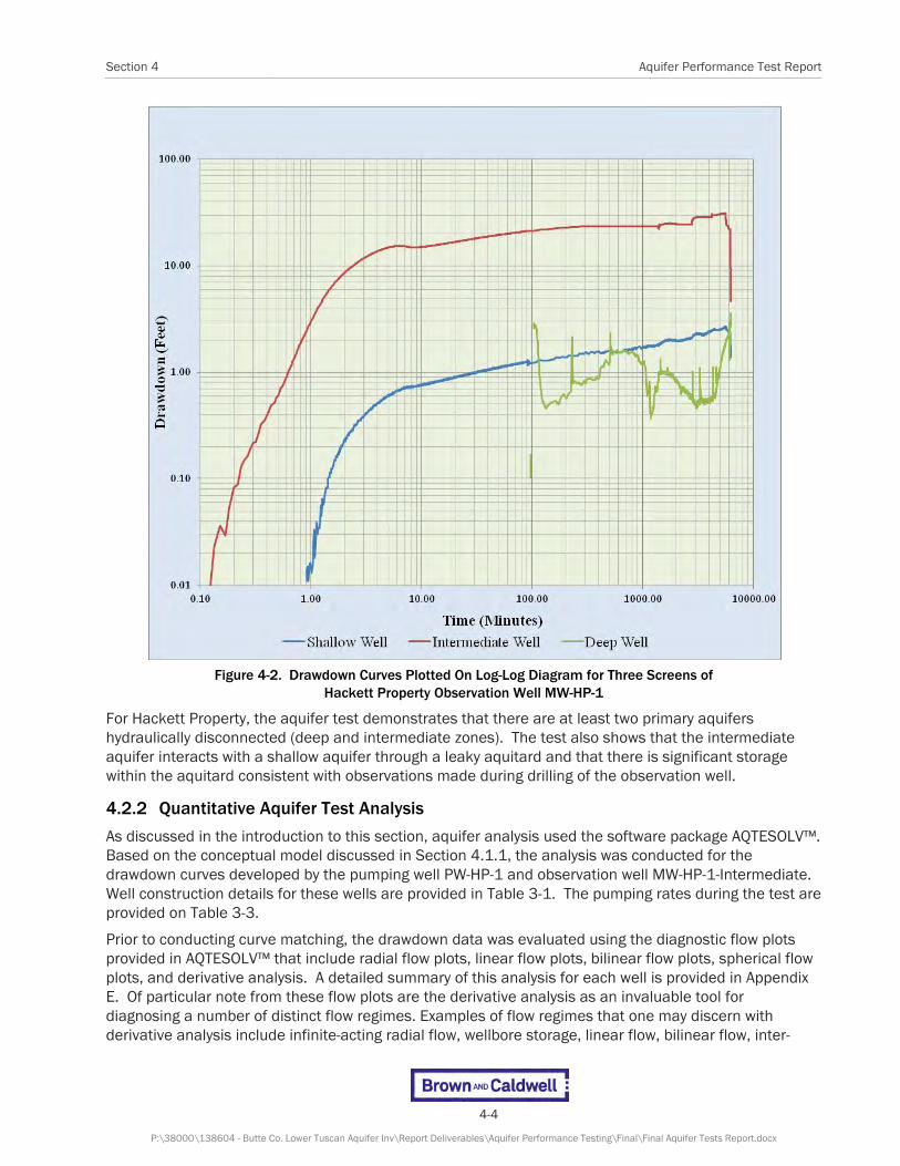
Section 4 Aquifer Performance Test Report
4-4
P:\38000\138604 - Butte Co. Lower Tuscan Aquifer Inv\Report Deliverables\Aquifer Performance Testing\Final\Final Aquifer Tests Report.docx
Figure 4-2. Drawdown Curves Plotted On Log-Log Diagram for Three Screens of
Hackett Property Observation Well MW-HP-1
For Hackett Property, the aquifer test demonstrates that there are at least two primary aquifers hydraulically disconnected (deep and intermediate zones). The test also shows that the intermediate aquifer interacts with a shallow aquifer through a leaky aquitard and that there is significant storage within the aquitard consistent with observations made during drilling of the observation well.
4.2.2 Quantitative Aquifer Test Analysis
As discussed in the introduction to this section, aquifer analysis used the software package AQTESOLV™. Based on the conceptual model discussed in Section 4.1.1, the analysis was conducted for the drawdown curves developed by the pumping well PW-HP-1 and observation well MW-HP-1-Intermediate. Well construction details for these wells are provided in Table 3-1. The pumping rates during the test are provided on Table 3-3.
Prior to conducting curve matching, the drawdown data was evaluated using the diagnostic flow plots provided in AQTESOLV™ that include radial flow plots, linear flow plots, bilinear flow plots, spherical flow plots, and derivative analysis. A detailed summary of this analysis for each well is provided in Appendix E. Of particular note from these flow plots are the derivative analysis as an invaluable tool for diagnosing a number of distinct flow regimes. Examples of flow regimes that one may discern with derivative analysis include infinite-acting radial flow, wellbore storage, linear flow, bilinear flow, inter-
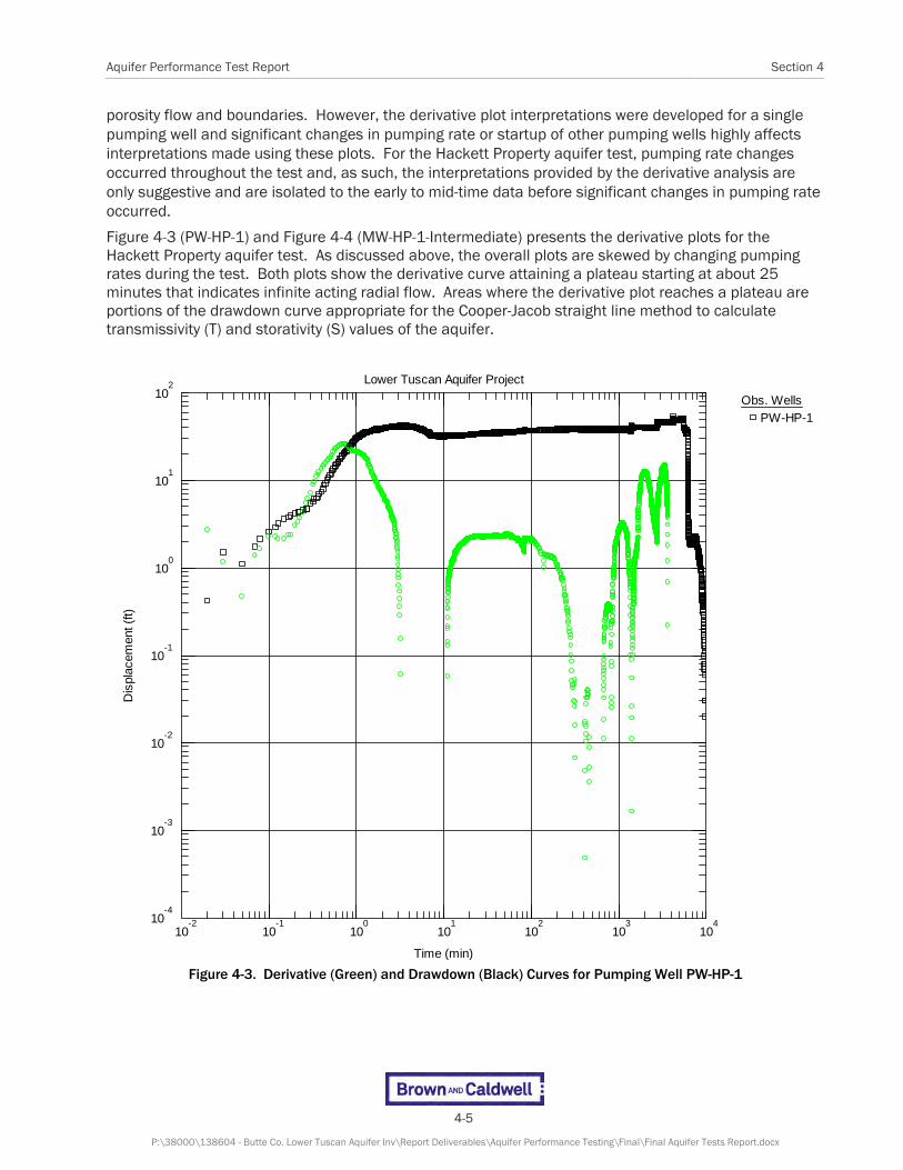
Aquifer Performance Test Report Section 4
4-5
P:\38000\138604 - Butte Co. Lower Tuscan Aquifer Inv\Report Deliverables\Aquifer Performance Testing\Final\Final Aquifer Tests Report.docx
porosity flow and boundaries. However, the derivative plot interpretations were developed for a single pumping well and significant changes in pumping rate or startup of other pumping wells highly affects interpretations made using these plots. For the Hackett Property aquifer test, pumping rate changes occurred throughout the test and, as such, the interpretations provided by the derivative analysis are only suggestive and are isolated to the early to mid-time data before significant changes in pumping rate occurred.
Figure 4-3 (PW-HP-1) and Figure 4-4 (MW-HP-1-Intermediate) presents the derivative plots for the Hackett Property aquifer test. As discussed above, the overall plots are skewed by changing pumping rates during the test. Both plots show the derivative curve attaining a plateau starting at about 25 minutes that indicates infinite acting radial flow. Areas where the derivative plot reaches a plateau are portions of the drawdown curve appropriate for the Cooper-Jacob straight line method to calculate transmissivity (T) and storativity (S) values of the aquifer.
Figure 4-3. Derivative (Green) and Drawdown (Black) Curves for Pumping Well PW-HP-1
Lower Tuscan Aquifer Project
10-2
10-1
100
101
102
103
10410
-4
10-3
10-2
10-1
100
101
102
Time (min)
Dis
plac
emen
t (ft)
Obs. Wells
PW-HP-1

Section 4 Aquifer Performance Test Report
4-6
P:\38000\138604 - Butte Co. Lower Tuscan Aquifer Inv\Report Deliverables\Aquifer Performance Testing\Final\Final Aquifer Tests Report.docx
Figure 4-4. Derivative (Green) and Drawdown (Red) Curves for Observation Well MW-HP-1-Intermediate
Early data (between 0.01 minute and 10 minutes) for the pumping well (Figure 4-3) is suggestive of wellbore storage effects. Accounting for the distortion due to changes in pumping rate, the shape of the derivative curve for the observation well intermediate screen (Figure 4-4) between 1 minute and 400 minutes could be interpreted as follows:
1. A well in an infinite leaky confined aquifer assuming a partially or fully penetrating line-source
pumping well, an incompressible aquitard, and a constant-head source aquifer. Derivative plateau at intermediate time indicates infinite-acting radial flow before drawdown departs from the Theis solution for a nonleaky confined aquifer.
2. A well in an infinite leaky confined aquifer assuming a fully penetrating line-source pumping well,
a compressible aquitard, and a constant-head source aquifer. Derivative plateau at intermediate time indicates infinite-acting radial flow before drawdown departs from the Theis solution for a nonleaky confined aquifer.
3. A well in a bounded nonleaky confined aquifer assuming a partially penetrating line source pumping well and a constant-head (recharge) boundary. Derivative plateau at intermediate time indicates infinite-acting radial flow. Recharge boundary produces constant drawdown at late time.
Lower Tuscan Aquifer Project
10-2
10-1
100
101
102
103
10410
-3
10-2
10-1
100
101
102
Time (min)
Dis
plac
emen
t (ft)
Obs. Wells
MW-HP-1-Intermediate

Aquifer Performance Test Report Section 4
4-7
P:\38000\138604 - Butte Co. Lower Tuscan Aquifer Inv\Report Deliverables\Aquifer Performance Testing\Final\Final Aquifer Tests Report.docx
Item 1 above bests fits the conceptual model presented in Section 4.2.1 that is supported by the response of observation well MW-HP-1 shallow screen well to pumping that suggests leakage through the overlying aquitard. As such, curve matching solutions used for quantitative analysis of T and S values were those that assumed a leaky confined aquifer system. Both the pumping well and observation well are assumed to be fully penetrating.
As discussed above, areas where the derivative plot reaches a plateau are portions of the drawdown curve appropriate for the Cooper-Jacob straight line method to calculate T and S values of the aquifer. T and S values calculated using this method represent preliminary estimates that are useful in constraining the analysis of the drawdown curves using other solutions. Derivative plots for both the pumping well (Figure 4-3) and observation well (Figure 4-4) show the derivative curve attaining a plateau starting at about 25 minutes indicating infinite acting radial flow. The Cooper-Jacob straight line solution for the pumping well and observation well intermediate screen over this portion of the plots are presented on Figures 4-5 and 4-6 respectively.
Figure 4-5. Cooper-Jacob Straight Solution for Pumping Well PW-HP-1
Straight line plotted over area representing plateau on derivative plot presented on Figure 4-3.
Lower Tuscan Aquifer Project
10-2
10-1
100
101
102
103
1040.
12.
24.
36.
48.
60.
Adjusted Time (min)
Dis
plac
emen
t (ft)
Obs. Wells
PW-HP-1
Aquifer Model
Confined
Solution
Cooper-Jacob
Parameters
T = 5150.7 ft2/dayS = 0.0006914

Section 4 Aquifer Performance Test Report
4-8
P:\38000\138604 - Butte Co. Lower Tuscan Aquifer Inv\Report Deliverables\Aquifer Performance Testing\Final\Final Aquifer Tests Report.docx
Figure 4-6. Cooper-Jacob Straight Solution for Observation Well MW-HP-1 Intermediate Screen
Straight line plotted over area representing plateau on derivative plot presented on Figure 4-4.
As seen on these figures, T values calculated using the Cooper-Jacob straight method are 4,066 ft2/day (observation well) to 5,151 ft2/day (pumping well) and the S value for the observation well is 0.00003 (S values calculated from pumping well are inaccurate). Using an aquifer thickness of 35 feet shown on Figure 4-1, K values calculated from this method are 116 ft/day to 147 ft/day indicating well sorted sands or sand and gravel units. The geologic well log produced for observation well MW-HP-1 indicates this aquifer zone consists of sandy gravels to gravelly sands. The sieve analysis results collected from 330 feet bgs reported 12.5 percent gravels, 85.5 percent sand, and 1.9 percent fines. The calculated S value supports the intepretation that this aquifer is confined.
Moench (1985) derived a solution for unsteady flow to a fully penetrating, finite-diameter well with wellbore storage and wellbore skin in a homogeneous, isotropic leaky confined aquifer. In AQTESOLVE™, there are three configurations for simulating a leaky confined aquifer with aquitard storage for this method as follows: Case 1 assumes constant-head source aquifers supply leakage across overlying and underlying
aquitards.
Case 2 replaces both constant-head boundaries in Case 1 with no-flow boundaries Case 3 replaces the underlying constant-head boundary in Case 1 with a no-flow boundary.
Based on the conceptual model described above and response of the observation wells in the overlying (MW-HP-1 Shallow – delayed drawdown) and underlying (MW-HP-1-Deep, no response) aquifers, Case 3
Lower Tuscan Aquifer Project
10-2
10-1
100
101
102
103
1040.
8.
16.
24.
32.
40.
Adjusted Time (min)
Dis
plac
emen
t (ft)
Obs. Wells
MW-HP-1-Intermediate
Aquifer ModelConfined
Solution
Cooper-Jacob
Parameters
T = 4066.3 ft2/dayS = 2.916E-5

Aquifer Performance Test Report Section 4
4-9
P:\38000\138604 - Butte Co. Lower Tuscan Aquifer Inv\Report Deliverables\Aquifer Performance Testing\Final\Final Aquifer Tests Report.docx
best represents conditions of the aquifer test performed on the Hackett property. Figure 4-7 presents the Moench (1985) Case 3 solution for observation well MW-HP-1 intermediate. As seen on this plot, this configuration shows a relatively good fit for the early time and late time data and is considered the best estimate of T and S values for the aquifer zone analyzed by the Hackett Property aquifer test. Table 4-1 summarizes the T, S, and K (assuming aquifer thickness of 35 feet) values calculated using this method from the pumping and observation well including values calculated from the recovery tests (Appendix E). Appendix E also summarizes the assumptions of other analytical solutions used for analysis of the drawdown data.
Figure 4-7. Moench (1985) Case 3 Solution For Drawdown Curve Produced For Observation Well MW-HP-1
Intermediate Screen Interval During Hackett Property Aquifer Test
Table 4-1. Summary of T, S, and K values from Moench (1985) solution, Hackett Property aquifer test.
Well I.D.
Pumping Test Analysis Recovery Analysis
T (ft2/day)
S (unitless)
K (ft/day)
T (ft2/day)
S (unitless)
K (ft/day)
PW-HP-1 3555 Na 102 1388 na 40
MW-HP-1 Intermediate 2322 0.00004 66 3078 0.00009 88
Lower Tuscan Aquifer Project
10-2
10-1
100
101
102
103
10410
-2
10-1
100
101
102
Time (min)
Dis
plac
emen
t (ft)
Obs. Wells
MW-HP-1-Intermediate
Aquifer Model
Leaky
Solution
Moench (Case 3)
Parameters
T = 2321.9 ft2/dayS = 3.606E-5r/B' = 0.1139ß' = 0.1081r/B" = 0.ß" = 0.Sw = 0.r(w) = 0.5833 ftr(c) = 0.3333 ft

Section 4 Aquifer Performance Test Report
4-10
P:\38000\138604 - Butte Co. Lower Tuscan Aquifer Inv\Report Deliverables\Aquifer Performance Testing\Final\Final Aquifer Tests Report.docx
The reported K values listed in Table 4-1 are consistent with the sandy gravel unit reported for the aquifer unit observed at 340 feet to 360 feet within the MW-HP-1 soil boring. Reported S values for the observation well are consistent with the interpretation of a confined aquifer.
Neuman and Witherspoon (1969) derived a solution for unsteady flow to a fully penetrating well in a confined two-aquifer system. The method allows analyzing data from wells screened in the pumped aquifer, unpumped aquifer or aquitard. Wells in the aquifers are assumed to be fully penetrating; wells in the aquitard may be partially penetrating. This method was used for the Hackett Property aquifer test to provide order of magnitude estimates for T values within the shallow aquifer system.
Figure 4-8 presents the curve solution for observation well MW-HP-1-Intermediate/Shallow using the Neuman and Witherspoon Method. As seen on this figure, the curve solution for the pumped aquifer observation well (MW-HP-1-Intermediate) shows a very good fit for both early time and late time data whereas the curve solution for the unpumped aquifer (MW-HP-1-Shallow) shows a relatively good fit for early time and late time data
Figure 4-8. Neuman-Witherspoon Solution for MW-HP-1 Intermediate/Shallow Screen Zones
The method also assumes that the aquitard or confining bed has infinite areal extent, and uniform vertical hydraulic conductivity, storage coefficient, and thickness. As indicated above, the method also does not account for wellbore storage. Actual observations indicate that the confining bed is very heterogeneous and the unpumped observation well is not fully penetrating. As such, T values calculated for the unpumped aquifer and K values calculated for the aquitard are considered only estimates. The S
Lower Tuscan Aquifer Project
10-2
10-1
100
101
102
103
104
10510
-2
10-1
100
101
102
Time (min)
Dis
plac
emen
t (ft)
Obs. Wells
MW-HP-1-IntermediateMW-HP-1-Shallow
Aquifer Model
Leaky
Solution
Neuman-Witherspoon
Parameters
T = 1181. ft2/dayS = 9.0E-51/B = 0.002749 ft-1
ß/r = 0.000379 ft-1
T2 = 5.613E+4 ft2/dayS2 = 8.0E-9
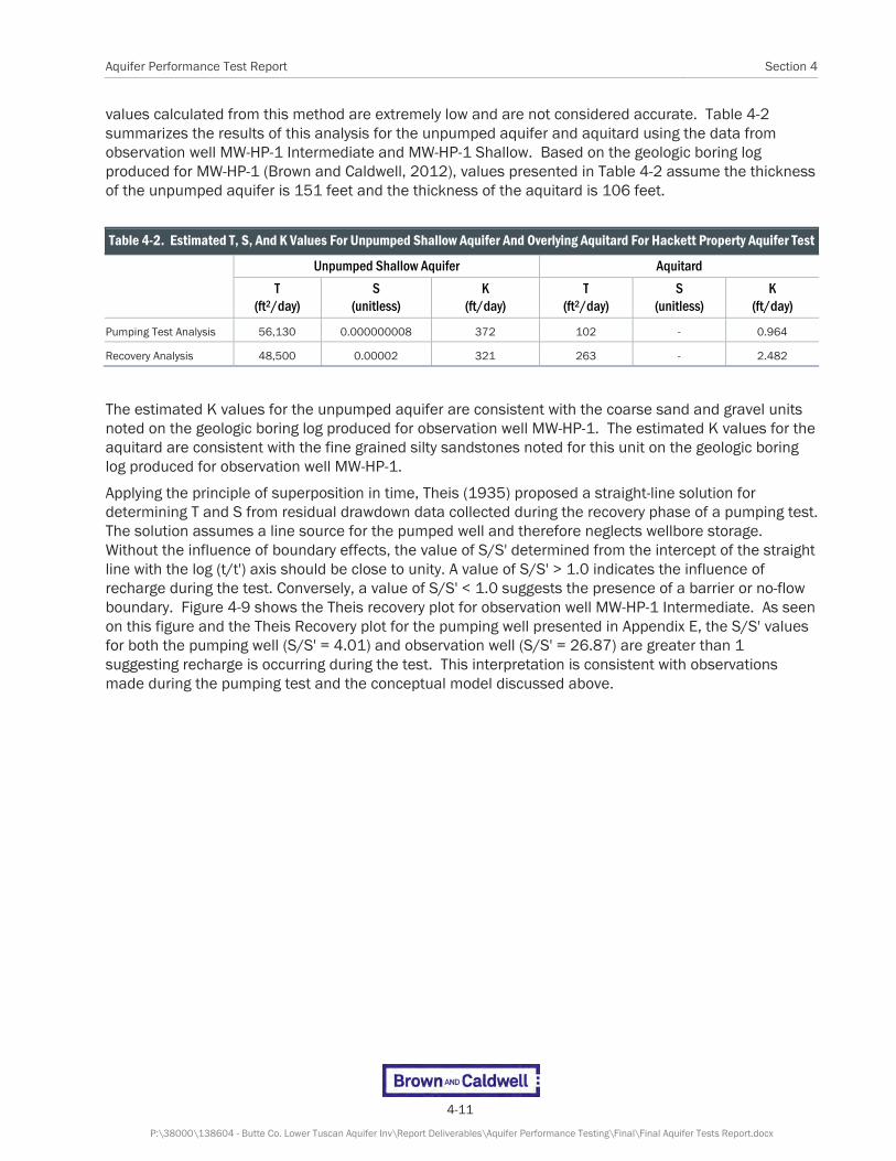
Aquifer Performance Test Report Section 4
4-11
P:\38000\138604 - Butte Co. Lower Tuscan Aquifer Inv\Report Deliverables\Aquifer Performance Testing\Final\Final Aquifer Tests Report.docx
values calculated from this method are extremely low and are not considered accurate. Table 4-2 summarizes the results of this analysis for the unpumped aquifer and aquitard using the data from observation well MW-HP-1 Intermediate and MW-HP-1 Shallow. Based on the geologic boring log produced for MW-HP-1 (Brown and Caldwell, 2012), values presented in Table 4-2 assume the thickness of the unpumped aquifer is 151 feet and the thickness of the aquitard is 106 feet.
Table 4-2. Estimated T, S, And K Values For Unpumped Shallow Aquifer And Overlying Aquitard For Hackett Property Aquifer Test
Unpumped Shallow Aquifer Aquitard
T (ft2/day)
S (unitless)
K (ft/day)
T (ft2/day)
S (unitless)
K (ft/day)
Pumping Test Analysis 56,130 0.000000008 372 102 - 0.964
Recovery Analysis 48,500 0.00002 321 263 - 2.482
The estimated K values for the unpumped aquifer are consistent with the coarse sand and gravel units noted on the geologic boring log produced for observation well MW-HP-1. The estimated K values for the aquitard are consistent with the fine grained silty sandstones noted for this unit on the geologic boring log produced for observation well MW-HP-1.
Applying the principle of superposition in time, Theis (1935) proposed a straight-line solution for determining T and S from residual drawdown data collected during the recovery phase of a pumping test. The solution assumes a line source for the pumped well and therefore neglects wellbore storage. Without the influence of boundary effects, the value of S/S' determined from the intercept of the straight line with the log (t/t') axis should be close to unity. A value of S/S' > 1.0 indicates the influence of recharge during the test. Conversely, a value of S/S' < 1.0 suggests the presence of a barrier or no-flow boundary. Figure 4-9 shows the Theis recovery plot for observation well MW-HP-1 Intermediate. As seen on this figure and the Theis Recovery plot for the pumping well presented in Appendix E, the S/S' values for both the pumping well (S/S' = 4.01) and observation well (S/S' = 26.87) are greater than 1 suggesting recharge is occurring during the test. This interpretation is consistent with observations made during the pumping test and the conceptual model discussed above.

Section 4 Aquifer Performance Test Report
4-12
P:\38000\138604 - Butte Co. Lower Tuscan Aquifer Inv\Report Deliverables\Aquifer Performance Testing\Final\Final Aquifer Tests Report.docx
Figure 4-9. Theis Recovery Plot for Observation Well MW-HP-1 Intermediate
Value of S/S’ greater than one suggests that recharge is occurring during the test.
4.3 M&T Ranch Aquifer Test Analysis This section summarizes the analysis of the aquifer test conducted between July 11, 2012 and July 15, 2012 at the M&T Ranch (Figures 1-1 and 3-4).
4.3.1 Conceptual Hydrogeologic Model
The aquifer test completed at the M&T Ranch was conducted in aquifers formed within the distal portion of the LTA composed predominantly of unconsolidated fluvial material. The hard cemented lahar units noted in the Hackett Property area are not as prevalent in this area. Overlying the LTA are approximately 160 feet of quaternary deposits formed by the ancestral movement of the Sacramento River system. A generalized geologic cross section developed using the lithologic logs produced from the observation (MW-MT-1) and pumping well (PW-MT-1) for this test is presented on Figure 4-10.
Three separate well screens were constructed within the observation well to monitor zones within both the Upper and Lower Tuscan Aquifers. The pumping well, PW-MT-1, is reported to be screened within the same sand zone of the shallow screen for the observation well between 280 and 400 feet bgs. The intermediate well screen was placed within the lower permeable fine grain units between the aquifers screened by the shallow and deep well screens. This design allowed assessment of the interaction
Lower Tuscan Aquifer Project
100
101
102
103
104
105
1060.
8.
16.
24.
32.
40.
Time, t/t'
Res
idua
l Dra
wdo
wn
(ft)
Obs. Wells
MW-HP-1-Intermediate
Aquifer Model
Confined
Solution
Theis (Recovery)
Parameters
T = 4026. ft2/dayS/S' = 26.87

Aquifer Performance Test Report Section 4
4-13
P:\38000\138604 - Butte Co. Lower Tuscan Aquifer Inv\Report Deliverables\Aquifer Performance Testing\Final\Final Aquifer Tests Report.docx
between the aquifers and a more detailed assessment of leakage responses through the low permeability units. The deep zone for this aquifer test is the same aquifer zone described in Section 3-2 tested by DWR in 1996.
Figure 4-10. Generalized Geologic Cross Section, M&T Ranch Aquifer Test. Pumping Well, PW-MT-1.
Observation Well, MW-MT-1.
The aquifer test was conducted for approximately 105 hours from July 11, 2012 to July 15, 2012. The pumping well used for the test was connected to an irrigation distribution system and the water extracted was used for normal irrigation (drip irrigation) practices of an almond orchard. As with the Hackett Property aquifer test, several line changes were made to irrigate different portions of the orchard that resulted in changes in the pumping rate during the test. The flow rates for the aquifer test ranged between 1,615 gpm to 1,850 gpm. Two other wells operated during the test, PW-MT-3 located

Section 4 Aquifer Performance Test Report
4-14
P:\38000\138604 - Butte Co. Lower Tuscan Aquifer Inv\Report Deliverables\Aquifer Performance Testing\Final\Final Aquifer Tests Report.docx
approximately 0.4 miles west of the pumping well and PW-MT-2 located approximately 1 mile north-northeast of the pumping well (Figure 3-4). PW-MT-3 operated for approximately 43 hours from June 12, 2012 to June 14, 2012 at rates ranging from 1,602 gpm to 1,690 gpm. PW-MT-2 operated for approximately 27 hours from July 11, 2012 to July 12, 2012 and 28 hours from July 14, 2012 to the end of the test on July 15, 2012. The pumping rate for PW-MT-2 averaged about 1,590 gpm. The two other wells monitored during the test, PW-MT-4 and PW-MT-5 (Figure 3-4) did not operate during the test.
Figure 4-11 shows the drawdown curves developed for the three screen intervals within the observation well during the aquifer test. These drawdown curves demonstrate that all three zones follow common radial flow drawdown patterns. The shallow well drawdown curve shows a slight delayed response (within 10 seconds) to the onset of pumping, changes in the pumping rate during modifications to irrigation of the orchard, and the turning on and off of PW-MT-3.
Figure 4-11. Drawdown Curves Plotted on Log-Log Diagram for Three Observation Well Screens within MW-MT-1
Used for M&T Ranch Aquifer Test
Both the intermediate and deep well drawdown curves also show a delayed response but the first response is a rise in water level at approximately two minutes after the onset of pumping. This response cannot be seen on Figure 4-11 that plots drawdown on a logarithmic scale (negative numbers do not plot on logarithmic scales). To illustrate the rise in water levels, Figure 4-12 presents the drawdown curves

Aquifer Performance Test Report Section 4
4-15
P:\38000\138604 - Butte Co. Lower Tuscan Aquifer Inv\Report Deliverables\Aquifer Performance Testing\Final\Final Aquifer Tests Report.docx
for the intermediate and deep wells plotted on a semi-log plot with drawdown on a linear scale. The effect of rising water levels in response to pumping was first recognized by Verruijt (1969) who concluded that the reverse well fluctuations occurred because pumping instantly compressed the aquifer to force water up the well. Verruijt (1969) referred to this response as the Noordbergum effect.
Figure 4-12. Drawdown Curves Plotted for Intermediate and Deep Well Screens of
Observation Well MW-MT-1 on Semi-Log Diagram
For this region, the aquifer test demonstrates that there are at least two primary aquifers hydraulically connected within the Tuscan Formation (shallow and deep zones) and that there is significant storage within the aquitard separating these zones.
4.3.2 Quantitative Aquifer Test Analysis
Based on the conceptual model discussed in Section 4.3.1, the analysis was conducted for the drawdown curves developed by the pumping well PW-MT-1 and observation well MW-MT-1-Shallow. Well construction details for these wells are provided in Table 3-5. The pumping rates during the test are provided on Table 3-7.
A detailed summary of the diagnostic flow plot analyses conducted for the M&T Ranch aquifer test is provided in Appendix E. For this aquifer test, pumping rate changes occurred throughout the test and, as
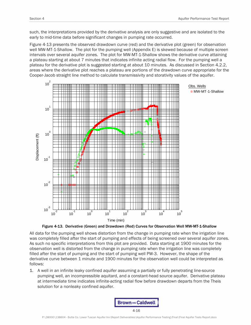
Section 4 Aquifer Performance Test Report
4-16
P:\38000\138604 - Butte Co. Lower Tuscan Aquifer Inv\Report Deliverables\Aquifer Performance Testing\Final\Final Aquifer Tests Report.docx
such, the interpretations provided by the derivative analysis are only suggestive and are isolated to the early to mid-time data before significant changes in pumping rate occurred.
Figure 4-13 presents the observed drawdown curve (red) and the derivative plot (green) for observation well MW-MT-1-Shallow. The plot for the pumping well (Appendix E) is skewed because of multiple screen intervals over several aquifer zones. The plot for MW-MT-1-Shallow shows the derivative curve attaining a plateau starting at about 7 minutes that indicates infinite acting radial flow. For the pumping well a plateau for the derivative plot is suggested starting at about 10 minutes. As discussed in Section 4.2.2, areas where the derivative plot reaches a plateau are portions of the drawdown curve appropriate for the Cooper-Jacob straight line method to calculate transmissivity and storativity values of the aquifer.
Figure 4-13. Derivative (Green) and Drawdown (Red) Curves for Observation Well MW-MT-1-Shallow
All data for the pumping well shows distortion from the change in pumping rate when the irrigation line was completely filled after the start of pumping and effects of being screened over several aquifer zones. As such no specific interpretations from this plot are provided. Data starting at 1900 minutes for the observation well is distorted from the change in pumping rate when the irrigation line was completely filled after the start of pumping and the start of pumping well PW-3. However, the shape of the derivative curve between 1 minute and 1900 minutes for the observation well could be interpreted as follows:
1. A well in an infinite leaky confined aquifer assuming a partially or fully penetrating line-source pumping well, an incompressible aquitard, and a constant-head source aquifer. Derivative plateau at intermediate time indicates infinite-acting radial flow before drawdown departs from the Theis solution for a nonleaky confined aquifer.
10-2
10-1
100
101
102
103
104
10510
-3
10-2
10-1
100
101
102
Time (min)
Dis
plac
emen
t (f
t)
Obs. Wells
MW-MT-1-Shallow

Aquifer Performance Test Report Section 4
4-17
P:\38000\138604 - Butte Co. Lower Tuscan Aquifer Inv\Report Deliverables\Aquifer Performance Testing\Final\Final Aquifer Tests Report.docx
2. A well in an infinite leaky confined aquifer assuming a fully penetrating line-source pumping well, a compressible aquitard, and a constant-head source aquifer.
Item 1 above best fits the conceptual model presented in Section 4.2.1 that is supported by the response of observation well MW-HP-1 intermediate and deep screened wells to pumping that suggest leakage through the underlying aquitard and hydraulic connection to the deep aquifer. As such, curve matching solutions used for quantitative analysis of T and S values were those that assumed a leaky confined aquifer system. Both the pumping well and observation well are assumed to be fully penetrating.
As discussed above, areas where the derivative plot reaches a plateau are portions of the drawdown curve appropriate for the Cooper-Jacob straight line method to calculate transmissivity and storativity values of the aquifer. T and S values calculated using this method represent preliminary estimates that are useful in constraining the analysis of the drawdown curves using other solutions. Derivative plots for both the pumping well (Appendix E) and observation well (Figure 4-12) show the derivative curve attaining a plateau starting at about 10 minutes and 7 minutes, respectively, indicating infinite acting radial flow. The Cooper-Jacob straight line solution for the observation well shallow screen over this portion of the plot is presented on Figure 4-14.
Figure 4-14. Cooper-Jacob Straight Solution for Observation Well MW-MT-1 Shallow Screen
Straight line plotted over area representing plateau on derivative plot presented on Figure 4-12.
The T values calculated using the Cooper-Jacob straight method are 9,399 ft2/day (pumping well) and 15,050 ft2/day (observation well) and the S value for the observation well is 0.0005. Using an aquifer thickness of 36 feet, K values calculated from this method are 261 ft/day to 418 ft/day indicating a sand and gravel unit. The geologic well log produced for observation well MW-MT-1 indicates this aquifer
10-2
10-1
100
101
102
103
104
1050.
4.
8.
12.
16.
20.
Adjusted Time (min)
Dis
plac
emen
t (ft)
Obs. Wells
MW-MT-1-Shallow
Aquifer Model
Confined
Solution
Cooper-Jacob
Parameters
T = 1.505E+4 ft2/dayS = 0.0005284

Section 4 Aquifer Performance Test Report
4-18
P:\38000\138604 - Butte Co. Lower Tuscan Aquifer Inv\Report Deliverables\Aquifer Performance Testing\Final\Final Aquifer Tests Report.docx
zone consists of sandy gravels to a conglomerate (clasts noted in drill cuttings up to 6-inches in diameter). The sieve analysis for the sample collected from 370 feet bgs reported 68.7 percent gravel, 28.7 percent sand, and 2.6 percent fines. The calculated S value supports the interpretation that this aquifer is confined.
Based on the conceptual model described in Section 4.3.1 and response of the observation wells in the underlying aquitard (MW-MT-1-intermediate) and deep aquifer (MW-MT-1-deep), Moench (1985) Case 1 (constant-head source aquifers supply leakage across overlying and underlying aquitards) best represents conditions of the aquifer test performed at the M&T Ranch. Figure 4-15 presents the Moench (1985) Case 1 solution for observation well MW-MT-1 shallow. As seen on this plot, this configuration shows a relatively good fit for the early time and late time data and is considered the best estimate of T and S values for the aquifer zone analyzed by the M&T Ranch aquifer test. Table 4-3 summarizes the T, S, and K (assuming aquifer thickness of 36 feet) values calculated using this method from the pumping and observation well including values calculated from the recovery tests (Appendix E). Also included on this table are the estimated T and S values using the two aquifer Neuman-Witherspoon (1969) solution for the DWR (1996) aquifer test discussed in Section 2.2.4.
Figure 4-15. Moench (1985) Case 1 Solution for Observation Well MW-MT-1 Shallow, M&T Ranch Aquifer Test
10-2
10-1
100
101
102
103
104
10510
-2
10-1
100
101
102
Time (min)
Dis
plac
emen
t (ft)
Obs. Wells
MW-MT-1-Shallow
Aquifer Model
Leaky
Solution
Moench (Case 1)
Parameters
T = 1.155E+4 ft2/dayS = 0.0004537r/B' = 0.07976ß' = 0.0638r/B" = 0.ß" = 0.Sw = 0.r(w) = 1.167 ftr(c) = 0.6667 ft

Aquifer Performance Test Report Section 4
4-19
P:\38000\138604 - Butte Co. Lower Tuscan Aquifer Inv\Report Deliverables\Aquifer Performance Testing\Final\Final Aquifer Tests Report.docx
Table 4-3. Summary of T, S, and K Values from Moench (1985) Solution, M&T Ranch Aquifer Test and from Neuman-Witherspoon Solution for DWR (1996) Aquifer Test
Well I.D.
Pumping Test Analysis Recovery Analysis
T (ft2/day)
S (unitless)
K (ft/day)
T (ft2/day)
S (unitless)
K (ft/day)
PW-MT-1 4384 0.00005 122 18860 - 524
MW-MT-1 Shallow 11550 0.00045 321 20540 0.0003 571
DWR (1996) test results 21250 0.00001 590 - - -
The reported K values listed in Table 4-3 are consistent with the sandy gravel to conglomerate unit reported for the aquifer unit observed at 350 feet to 390 feet within the MW-MT-1 soil boring. Reported S values for the observation well are consistent with the interpretation of a confined aquifer.
Figure 4-16 shows the Neuman-Witherspoon (1969) solution for observation well MW-MT-1 Shallow for unsteady flow to a fully penetrating well in a confined two-aquifer system. The curve solution for this well shows a very good fit for both early time and late time data. Values for the unpumped aquifer represent the overlying aquifer where no observation wells occur. For the pumping well, convergence using the automatic fit would not occur and a visual best fit was poor. It is believed that this poor fit for this method is due to the fact that the pumping well has screen intervals within other aquifer zones.
Figure 4-16. Neuman-Witherspoon (1969) Solution for Observation Well MW-MT-1 Shallow, M&T Ranch Aquifer
Test. T2 and S2 Represent The T and S Values for the Unpumped Aquifer.
10-2
10-1
100
101
102
103
104
10510
-2
10-1
100
101
102
Time (min)
Dis
pla
cem
ent (
ft)
Obs. Wells
MW-MT-1-Shallow
Aquifer Model
Leaky
Solution
Neuman-Witherspoon
Parameters
T = 1.228E+4 ft2/dayS = 0.0005997r/B = 0.1794ß = 0.02046T2 = 2.533E+4 ft2/dayS2 = 0.0001

Section 4 Aquifer Performance Test Report
4-20
P:\38000\138604 - Butte Co. Lower Tuscan Aquifer Inv\Report Deliverables\Aquifer Performance Testing\Final\Final Aquifer Tests Report.docx
Table 4-4 summarizes the results of this analysis for the unpumped aquifer and aquitard using the data from observation well MW-MT-1 Shallow. Based on the geologic boring log produced for MW-MT-1 (Brown and Caldwell, 2012), values presented in Table 4-2 assume the thickness of the unpumped aquifer is 95 feet and the thickness of the aquitard is 387 feet.
Table 4-4. Estimated T, S, and K values for Unpumped Shallow Aquifer and Overlying Aquitard for M&T Ranch Aquifer Test
Unpumped Shallow Aquifer Aquitard
T (ft2/day)
S (unitless)
K (ft/day)
T (ft2/day)
S (unitless)
K (ft/day)
Pumping Test Analysis 25330 0.0001 266 1120 - 2.893
The estimated K value for the unpumped aquifer is consistent with the coarse sand and gravely sand units noted on the geologic boring log produced for observation well MW-MT-1. The estimated K value for the aquitard is consistent with the fine grained silty sandstones to fine grained sands noted for this unit on the geologic boring log produced for observation well MW-HP-1.
As seen on the Theis Recovery plots presented in Appendix E, the S/S' values for both the pumping well (S/S' = 2.171) and observation well (S/S' = 1.393) are greater than 1 suggesting recharge is occurring during the test. This interpretation is consistent with observations made during the pumping test and the conceptual model discussed above. Appendix E also summarizes the assumptions of other analytical solutions used for analysis of the drawdown data.
4.4 Esquon Ranch Aquifer Test This section summarizes the analysis of the aquifer tests conducted between May 5, 2011 and May 21, 2011 at the Esquon Ranch (Figures 1-1 and 3-5).
4.4.1 Conceptual Hydrogeologic Model
The aquifer test completed at the Esquon Ranch was conducted in aquifers formed within the distal portions of the Lower Tuscan Aquifer (LTA) composed predominantly of unconsolidated fluvial material but with some hard cemented reworked lahar units. The Lower Tuscan Formation was observed at the surface in this area. A generalized geologic cross section developed using the lithologic logs produced from the observation (MW-ESQ-1) and pumping wells (PW-ESQ-39 and PW-ESQ-40) for this test is presented on Figure 4-17. Figure 3-5 shows the location of these wells along with other irrigation wells that were monitored for this test. Four separate well screens were constructed within the observation well to monitor zones within the LTA (shallow, intermediate shallow and intermediate deep wells) and the underlying Ione Formation (deep well). The pumping wells, as illustrated on Figure 4-17, are reported to be screened across the entire interval monitored by both the intermediate shallow and intermediate deep wells between 110 and 520 feet bgs. The shallow, intermediate shallow and intermediate deep wells are placed within permeable sand units separated by low permeable fines and lahar units of the LTA. The deep well is placed within permeable sands of the Ione Formation that is overlain by low permeability fines and lahar units of the LTA. This design allowed assessment of the interaction between the aquifers of both the LTA and Ione Formation and an assessment of leakage responses through the low permeability units.

Aquifer Performance Test Report Section 4
4-21
P:\38000\138604 - Butte Co. Lower Tuscan Aquifer Inv\Report Deliverables\Aquifer Performance Testing\Final\Final Aquifer Tests Report.docx
Figure 4-17. Generalized geologic cross section, Esquon Ranch Aquifer Test. Tuscan Formation in this area is part of the LTA. Pumping Wells, PW-ESQ-39 and PW-ESQ-40. Observation Well, MW-ESQ-1.
Due to weather conditions, two separate aquifer tests were conducted at the Esquon Ranch. The first test was conducted for approximately 85 hours from May 5, 2011 to May 8, 2011. This pumping test consisted of turning on the first well, PW-ESQ-39 (Figure 3-5), followed by the second well, PW-ESQ-40, twenty four hours later on May 6, 2011. A second test was conducted from May 13, 2011 to May 21, 2011 for approximately 195 hours. Since the first test indicated that there was not significanct difference in response in the observation wells to turning on each of the wells individually this aquifer test consisted of turning on both pumping wells simultaneously.
The pumping wells used for the test were connected to an irrigation distribution system and the water extracted was used for normal irrigation (flood irrigation) practices of rice fields. The flow rates for the aquifer test ranged between 1,390 gpm to 1,780 gpm for PW-ESQ-39 and 1,165 gpm to 1,500 gpm for PW-ESQ-40. Sixteen other wells operated during the test with pumping rates ranging from 940 gpm to 2,605 gpm. Only four wells, PW-ESQ-12 (1,300 gpm), PW-ESQ-13 (1,200 gpm), PW-ESQ-16 (1,300 gpm), and PW-ESQ-22 (1,250 gpm) showed measurable effects to the drawdown curves produced for MW-ESQ-1. Figure 3-5 shows the location of these wells and their approximate distances from the observation well and pumping wells used for the test.
Figure 4-18 shows the drawdown curves developed for the four screen intervals within the observation well during the aquifer tests along with startup and shutdown times for each of the irrigation wells that affected the drawdown curves. Unlike the other drawdown curves presented above, this plot is

Section 4 Aquifer Performance Test Report
4-22
P:\38000\138604 - Butte Co. Lower Tuscan Aquifer Inv\Report Deliverables\Aquifer Performance Testing\Final\Final Aquifer Tests Report.docx
presented on a linear scale to highlight the differences in response between wells. The drawdown curves demonstrate that the two intermediate zones follow common radial flow drawdown patterns. Both of these well drawdown curves show delayed responses to the onset of pumping between 40 minutes (intermediate shallow) and 90 minutes (intermediate deep). Both wells also show responses to the other four pumping wells discussed above. The drawdown curve for the deep well showed a delayed response of approximately 1,000 minutes (16.5 hours) and the shape of the curve suggests that although hydraulically connected, water from this zone has to follow an indirect path to the zone of pumping used for the test. This observation is consistent with the geologic cross section illustrated on Figure 4-15 that shows this well completed within the Ione Formation beneath fine grained units of the Tuscan Formation and suggests that the sands of the Ione Formation in this area connect with the sands of the Tuscan Formation at a different location. The shallow zone drawdown curve indicates that this aquifer is not hydraulically connected with the lower zones. The shallow well did respond to pumping from PW-ESQ-22 (Figure 3-5).
For this region, the aquifer test demonstrates that the primary LTA aquifer is hydraulically connected to the aquifer within the upper Ione Formation but water from these two zones follow indirect pathways. The shallow aquifer zone of the LTA in this area is not hydraulically connected with the lower zone of the LTA.

Section 4 Aquifer Performance Test Report
4-23
P:\38000\138604 - Butte Co. Lower Tuscan Aquifer Inv\Report Deliverables\Aquifer Performance Testing\Final\Final Aquifer Tests Report.docx
Figure 4-18. Drawdown curves plotted on Semi-log diagram for four observation well screens within MW-ESQ-1 used for Esquon Ranch aquifer test. Figure also shows bars indicating startup and shutdown of irrigation wells, weather events that effected
the duration of the aquifer tests, and a brief evaluation of each of the curves with respect to validity for use in quantitative curve matching analysis.

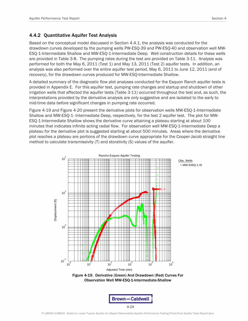
Aquifer Performance Test Report Section 4
4-24
P:\38000\138604 - Butte Co. Lower Tuscan Aquifer Inv\Report Deliverables\Aquifer Performance Testing\Final\Final Aquifer Tests Report.docx
4.4.2 Quantitative Aquifer Test Analysis
Based on the conceptual model discussed in Section 4.4.1, the analysis was conducted for the drawdown curves developed by the pumping wells PW-ESQ-39 and PW-ESQ-40 and observation well MW-ESQ-1-Intermediate Shallow and MW-ESQ-1-Intermediate Deep. Well construction details for these wells are provided in Table 3-8. The pumping rates during the test are provided on Table 3-11. Analysis was performed for both the May 6, 2011 (Test 1) and May 13, 2011 (Test 2) aquifer tests. In addition, an analysis was also performed over the entire aquifer test period, May 6, 2011 to June 12, 2011 (end of recovery), for the drawdown curves produced for MW-ESQ-Intermediate Shallow.
A detailed summary of the diagnostic flow plot analyses conducted for the Esquon Ranch aquifer tests is provided in Appendix E. For this aquifer test, pumping rate changes and startup and shutdown of other irrigation wells that affected the aquifer tests (Table 3-11) occurred throughout the test and, as such, the interpretations provided by the derivative analysis are only suggestive and are isolated to the early to mid-time data before significant changes in pumping rate occurred.
Figure 4-19 and Figure 4-20 present the derivative plots for observation wells MW-ESQ-1-Intermediate Shallow and MW-ESQ-1- Intermediate Deep, respectively, for the test 2 aquifer test. The plot for MW-ESQ-1-Intermediate Shallow shows the derivative curve attaining a plateau starting at about 100 minutes that indicates infinite acting radial flow. For observation well MW-ESQ-1-Intermediate Deep a plateau for the derivative plot is suggested starting at about 500 minutes. Areas where the derivative plot reaches a plateau are portions of the drawdown curve appropriate for the Cooper-Jacob straight line method to calculate transmissivity (T) and storativity (S) values of the aquifer.
Figure 4-19. Derivative (Green) And Drawdown (Red) Curves For
Observation Well MW-ESQ-1-Intermediate-Shallow
Rancho Esquon Aquifer Testing
100
101
102
103
104
10510
-1
100
101
102
Adjusted Time (min)
Dis
plac
emen
t (f
t)
Obs. Wells
MW-EWQ-1-IS
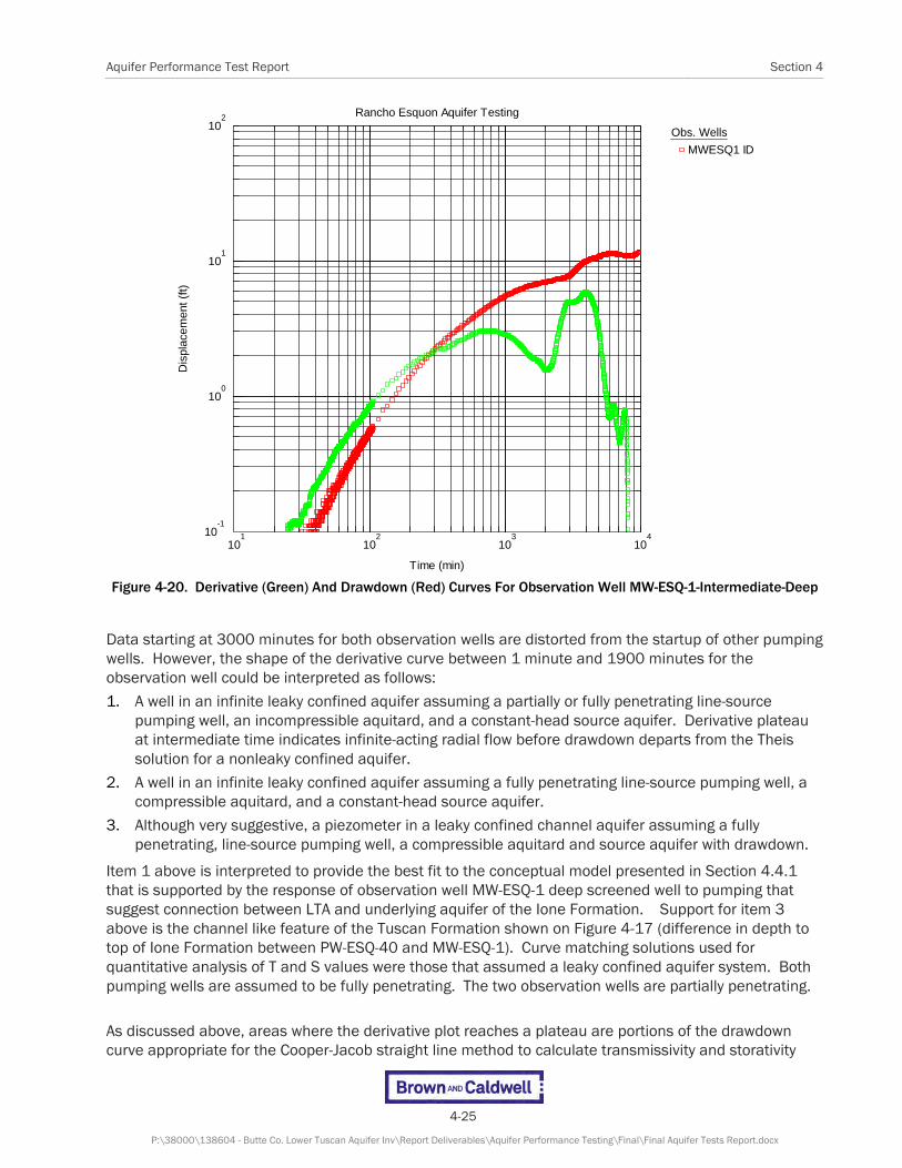
Aquifer Performance Test Report Section 4
4-25
P:\38000\138604 - Butte Co. Lower Tuscan Aquifer Inv\Report Deliverables\Aquifer Performance Testing\Final\Final Aquifer Tests Report.docx
Figure 4-20. Derivative (Green) And Drawdown (Red) Curves For Observation Well MW-ESQ-1-Intermediate-Deep
Data starting at 3000 minutes for both observation wells are distorted from the startup of other pumping wells. However, the shape of the derivative curve between 1 minute and 1900 minutes for the observation well could be interpreted as follows:
1. A well in an infinite leaky confined aquifer assuming a partially or fully penetrating line-source pumping well, an incompressible aquitard, and a constant-head source aquifer. Derivative plateau at intermediate time indicates infinite-acting radial flow before drawdown departs from the Theis solution for a nonleaky confined aquifer.
2. A well in an infinite leaky confined aquifer assuming a fully penetrating line-source pumping well, a compressible aquitard, and a constant-head source aquifer.
3. Although very suggestive, a piezometer in a leaky confined channel aquifer assuming a fully penetrating, line-source pumping well, a compressible aquitard and source aquifer with drawdown.
Item 1 above is interpreted to provide the best fit to the conceptual model presented in Section 4.4.1 that is supported by the response of observation well MW-ESQ-1 deep screened well to pumping that suggest connection between LTA and underlying aquifer of the Ione Formation. Support for item 3 above is the channel like feature of the Tuscan Formation shown on Figure 4-17 (difference in depth to top of Ione Formation between PW-ESQ-40 and MW-ESQ-1). Curve matching solutions used for quantitative analysis of T and S values were those that assumed a leaky confined aquifer system. Both pumping wells are assumed to be fully penetrating. The two observation wells are partially penetrating.
As discussed above, areas where the derivative plot reaches a plateau are portions of the drawdown curve appropriate for the Cooper-Jacob straight line method to calculate transmissivity and storativity
Rancho Esquon Aquifer Testing
101
102
103
10410
-1
100
101
102
Time (min)
Dis
plac
emen
t (ft)
Obs. Wells
MWESQ1 ID

Section 4 Aquifer Performance Test Report
4-26
P:\38000\138604 - Butte Co. Lower Tuscan Aquifer Inv\Report Deliverables\Aquifer Performance Testing\Final\Final Aquifer Tests Report.docx
values of the aquifer. T and S values calculated using this method represent preliminary estimates that are useful in constraining the analysis of the drawdown curves using other solutions. Derivative plots for the pumping wells during test 2 (Appendix E) show the derivative curve attaining a plateau starting at about 1 minute to 20 minutes indicating infinite acting radial flow. The observation wells (Figure 4-19 and 4-20) show the derivative curves attaining a plateau starting at about 100 minutes to 500 minutes for the test 2 aquifer test. Table 4-5 summarized the T, S, and K values calculated using the Cooper-Jacob straight line method for both test 1 and test 2. The K values are calculated assuming an aquifer thickness of 300 feet.
Table 4-5. T, S, and K Values Calculated Using Cooper-Jacob Straight Line Method for the
Esquon Ranch Test 1 And Test 2 Aquifer Tests
T
(ft2/day) S
(unitless) K
(ft/day)
Test 1
MW-ESQ-1-Intermediate Shallow 21,610 0.0003 72
MW-ESQ-1-Intermediate Deep 20,180 0.0006 67
PW-ESQ-39 16,650 - 56
PW-ESQ-40 17,750 - 59
Test 2
MW-ESQ-1-Intermediate Shallow 11,030 0.00009 37
MW-ESQ-1-Intermediate Deep 9,095 0.0003 30
PW-ESQ-39 18,700 - 62
PW-ESQ-40 10,860 - 36
During test 1, PW-ESQ-39 operated by itself for approximately 25 hours allowing for an estimate of T and S values using the distance-drawdown method. Wells used for this analysis included PW-ESQ-39, PW-ESQ-40, PW-ESQ-13, and PW-ESQ-16. Figure 4-21 shows the results of this analysis with reported T and S values of 11,737 ft2/day and 0.001, respectively. Using an aquifer thickness of 300 feet, the calculated K value for this method is 39 ft/day. This K value and those calculated using the Cooper-Jacob straight line method are indicative of well sorted sands. Based on the geologic well log produced by DWR for observation well MW-ESQ-1, well sorted sands occur in the zones screened by the intermediate shallow and intermediate deep screen intervals. Other zones within the aquifer zone tested are classified as sandstones.
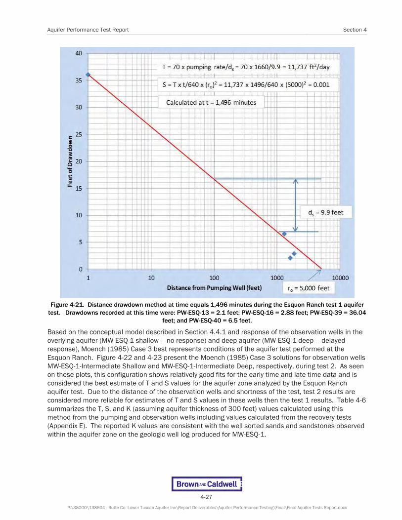
Aquifer Performance Test Report Section 4
4-27
P:\38000\138604 - Butte Co. Lower Tuscan Aquifer Inv\Report Deliverables\Aquifer Performance Testing\Final\Final Aquifer Tests Report.docx
Figure 4-21. Distance drawdown method at time equals 1,496 minutes during the Esquon Ranch test 1 aquifer
test. Drawdowns recorded at this time were: PW-ESQ-13 = 2.1 feet; PW-ESQ-16 = 2.88 feet; PW-ESQ-39 = 36.04 feet; and PW-ESQ-40 = 6.5 feet.
Based on the conceptual model described in Section 4.4.1 and response of the observation wells in the overlying aquifer (MW-ESQ-1-shallow – no response) and deep aquifer (MW-ESQ-1-deep – delayed response), Moench (1985) Case 3 best represents conditions of the aquifer test performed at the Esquon Ranch. Figure 4-22 and 4-23 present the Moench (1985) Case 3 solutions for observation wells MW-ESQ-1-Intermediate Shallow and MW-ESQ-1-Intermediate Deep, respectively, during test 2. As seen on these plots, this configuration shows relatively good fits for the early time and late time data and is considered the best estimate of T and S values for the aquifer zone analyzed by the Esquon Ranch aquifer test. Due to the distance of the observation wells and shortness of the test, test 2 results are considered more reliable for estimates of T and S values in these wells then the test 1 results. Table 4-6 summarizes the T, S, and K (assuming aquifer thickness of 300 feet) values calculated using this method from the pumping and observation wells including values calculated from the recovery tests (Appendix E). The reported K values are consistent with the well sorted sands and sandstones observed within the aquifer zone on the geologic well log produced for MW-ESQ-1.

Section 4 Aquifer Performance Test Report
4-28
P:\38000\138604 - Butte Co. Lower Tuscan Aquifer Inv\Report Deliverables\Aquifer Performance Testing\Final\Final Aquifer Tests Report.docx
Figure 4-22. Moench (1985) Case 3 solution for observation well MW-ESQ-1
Intermediate Shallow, Esquon Ranch test 2 aquifer test.
Rancho Esquon Aquifer Testing
100
101
102
103
104
10510
-1
100
101
102
Time (min)
Dis
plac
emen
t (ft)
Obs. Wells
MW-EWQ-1-IS
Aquifer Model
Leaky
Solution
Moench (Case 3)
Parameters
T = 2.365E+4 ft2/dayS = 0.0003053r/B' = 0.2002ß' = 1.0E-5r/B" = 0.ß" = 0.Sw = 0.r(w) = 1. ftr(c) = 0.6667 ft

Aquifer Performance Test Report Section 4
4-29
P:\38000\138604 - Butte Co. Lower Tuscan Aquifer Inv\Report Deliverables\Aquifer Performance Testing\Final\Final Aquifer Tests Report.docx
Figure 4-23. Moench (1985) Case 3 solution for observation well MW-ESQ-1 Intermediate Deep,
Esquon Ranch test 2 aquifer test.
Rancho Esquon Aquifer Testing
101
102
103
104
10510
-1
100
101
102
Time (min)
Dis
plac
emen
t (ft)
Obs. Wells
MWESQ1 ID
Aquifer Model
Leaky
Solution
Moench (Case 3)
Parameters
T = 1.771E+4 ft2/dayS = 0.0009565r/B' = 0.3943ß' = 0.0001594r/B" = 0.ß" = 0.Sw = 0.r(w) = 1. ftr(c) = 0.6667 ft

Section 4 Aquifer Performance Test Report
4-30
P:\38000\138604 - Butte Co. Lower Tuscan Aquifer Inv\Report Deliverables\Aquifer Performance Testing\Final\Final Aquifer Tests Report.docx
Table 4-6. Summary of T, S, and K Values from Moench (1985) Solution for Esquon Ranch Aquifer Test
T
(ft2/day) S
(unitless) K
(ft/day)
Test 1
Pumping
MW-ESQ-1-Intermediate Shallow 4013 0.00004 13
MW-ESQ-1-Intermediate Deep 2518 0.000004 8.4
PW-ESQ-39 12060 - 40
PW-ESQ-40 9773 - 33
Recovery
MW-ESQ-1-Intermediate Shallow 2000 0.00002 6.7
MW-ESQ-1-Intermediate Deep 515 000003 1.7
PW-ESQ-39 8446 - 28
PW-ESQ-40 3006 - 10
Test 2
Pumping
MW-ESQ-1-Intermediate Shallow 23650 0.0003 79
MW-ESQ-1-Intermediate Deep 17710 0.00096 59
PW-ESQ-39 7602 - 25
PW-ESQ-40 6152 - 21
Recovery
MW-ESQ-1-Intermediate Shallow 18770 0.0005 63
MW-ESQ-1-Intermediate Deep 12230 0.001 41
PW-ESQ-39 5826 - 19
PW-ESQ-40 6267 - 21
As seen on the Theis Recovery plots presented in Appendix E summarized on Table 4-7, the S/S' values for the pumping wells and observation wells during test 1 ranged from 0.0311 (MW-ESQ-1-Intermediate Deep) to 1.796 (PW-ESQ-39). Values greater than 1 suggest recharge is occurring during the test where conversely values less than 1 suggest the presence of a barrier or no-flow boundary. These observations during test 1 could represent the presence of a channel feature as observed on the geologic cross section presented on Figure 4-17 and could be the reason for the distinct differences in T and S values calculated during the two different tests. During test 2, all values were greater than 1 suggesting recharge was occurring during this recovery test in all zones monitored for the test. For test 2, this interpretation is consistent with observations made during the pumping test and the conceptual model discussed above. The variability between test 1 and test 2 suggest that heterogenities associated with channelized deposits potentially have limited extent and are affected by the duration differences.

Aquifer Performance Test Report Section 4
4-31
P:\38000\138604 - Butte Co. Lower Tuscan Aquifer Inv\Report Deliverables\Aquifer Performance Testing\Final\Final Aquifer Tests Report.docx
Table 4-7. Summary of S/S’ Values Calculated from Theis Recovery Method for Esquon Ranch Aquifer Test
Well I.D Test 1 Test 2
MW-ESQ-1-Intermediate Shallow 1.007 4.122
MW-ESQ-Intermediate Deep 0.0311 3.274
PW-ESQ-39 1.796 26.76
PW-ESQ-40 1.669 4.434
An analysis was also conducted on the drawdown curve produced for MW-ESQ-1-Intermediate Shallow during the entire period of test 1 and test 2. Figure 4-24 presents the Moench (1985) Case 3 solution for this analysis. As seen on this figure, this configuration shows relatively good fits for the early time and late time data and the T (19,990 ft2/day) and S (0.0002) values are consistent with the values calculated using the test 2 results. Appendix E also summarizes the assumptions of other analytical solutions used for analysis of the drawdown data.
Figure 4-24. Moench (1985) Case 3 solution for observation well MW-ESQ-1 Intermediate Shallow using
drawdown data from both test 1 and test 2 during the Esquon Ranch aquifer test.
Rancho Esquon Aquifer Testing
101
102
103
104
10510
-1
100
101
102
Time (min)
Dis
plac
emen
t (ft)
Obs. Wells
MW-ESQ-1IS
Aquifer Model
Leaky
Solution
Moench (Case 3)
Parameters
T = 1.999E+4 ft2/dayS = 0.0002221r/B' = 0.04422ß' = 0.09687r/B" = 0.ß" = 0.Sw = 0.r(w) = 1. ftr(c) = 0.6667 ft

5-1
P:\38000\138604 - Butte Co. Lower Tuscan Aquifer Inv\Report Deliverables\Aquifer Performance Testing\Final\Final Aquifer Tests Report.docx
Section 5
Groundwater Sampling As introduced in Section 3.4, groundwater samples were collected from each of the pumping wells used for the aquifer tests and submitted for analysis of cations, anions, and oxygen/deuterium? isotopes. The results of this testing is summarized in Table 5-1. A detailed discussion of these results in relationship to potential recharge areas for the aquifer will be presented within the Final Report.
Table 5-1. Summary of Groundwater Samples – LTA Aquifer Testing
Station PW-HP-1 PW-MT-1 PW-MT-2 PW-ESQ-39 PW-ESQ-40
Date Collected 6/24/2011 7/12/2012 7/12/2012 5/25/2011 5/25/2011
Anions Units
Total Alkalinity 99 170 180 110 110 mg/L
Bicarbonate as CaCO3 99 170 180 110 110 mg/L
Flouride NA 0.063 0.061 NA NA mg/L
Chloride 2.9 9.4 16 2.1 1.9 mg/L
Nitrate 12 3.2 3.6 1.3 0.55 mg/L
Nitrite as N <0.10 <0.10 <0.10 <0.10 <0.10 mg/L
Orthophosphate <0.15 0.1 <0.15 0.25 0.31 mg/L
Sulfate 7.6 6.6 7.5 0.92 0.82 mg/L
Sulfide <1.0 <1.0 <1.0 <1.0 <1.0 mg/L
Cations
Calcium 21 32 38 17 17 mg/L
Boron NA 0.077 0.087 NA NA mg/L
Iron <0.10 <0.10 <0.10 <0.10 <0.10 mg/L
Magnesium 14 22 25 13 14 mg/L
Manganese <0.02 <0.02 <0.02 0.11 0.16 mg/L
Potassium 16 2.1 1.8 1.8 2.1 mg/L
Sodium 8.6 14 16 8.1 8.6 mg/L
General Parameters
Specific Conductance 230 370 420 NA NA umhos/cm
Total Dissolved Solids 190 230 270 NA NA mg/L
pH 7.22 NA NA NA NA
Total Hardness as CaCO3 130 170 200 NA NA mg/L

Section 5 Aquifer Performance Test Report
5-2
P:\38000\138604 - Butte Co. Lower Tuscan Aquifer Inv\Report Deliverables\Aquifer Performance Testing\Final\Final Aquifer Tests Report.docx
Table 5-1. Summary of Groundwater Samples – LTA Aquifer Testing
Station PW-HP-1 PW-MT-1 PW-MT-2 PW-ESQ-39 PW-ESQ-40
Isotopes
δ18O -9 -9.9 -9.9 -8.6 -8.8 ‰
δD -64.9 -71.4 -71.8 -61.3 -62.2 ‰
Field Parameters
Temperature NA1 19.3 19.4 24.9 24.9 C
Specific Conductance NA1 359 419 208 194 umhos/cm
pH NA1 7.91 7.84 7.57 7.45 pH Units
1. Field Parameter not collected due to problem with field meter.
2. NA = Not Analyzed

6-1
P:\38000\138604 - Butte Co. Lower Tuscan Aquifer Inv\Report Deliverables\Aquifer Performance Testing\Final\Final Aquifer Tests Report.docx
Section 6
References Barlow, P.M., and Moench, A.F., 2011, WTAQ version 2—A computer program for analysis of aquifer tests in confined and
water-table aquifers with alternative representations of drainage from the unsaturated zone: U.S. Geological Survey Techniques and Methods 3-B9, 41 p.
Bear, J. (1972). Dynamics of Fluids in Porous Media. Dover Publications. ISBN 0-486-65675-6.
Blair, T.C., Baker, F.G., and Turner, J.B., 1991, Cenozoic Fluvial-Facies Architecture and Aquifer Heterogeneity, Oroville, California, Superfund Site and Vicinity, in A.D. Miall and N. Tyler, eds., The Three-Dimensional Facies Architecture of Terrigenous Clastic Sediments and Its Implications for Hydrocarbon Discovery and Recovery, SEPM, Concepts in Sedimentology and Paleontology, Volume 3, 1991.
Bourdet, D., Whittle, T.M., Douglas, A.A. and Y.M. Pirard, 1983, A new set of type curves simplifies well test analysis, World Oil, May 1983, pp. 95-106.
Bourdet, D., Ayoub, J.A. and Y.M. Pirard, 1989, Use of pressure derivative in well-test interpretation, SPE Formation Evaluation, June 1989, pp. 293-302.
Busacca, 1982, Geologic history and soil development, northeastern Sacramento Valley, California: Davis, University of California, Unpubl. Ph.D. Dissertation, 348 p.
Butte County, 2010, Initial Study/Proposed Mitigation Negative Declaration, Lower Tuscan Aquifer Monitoring, Recharge and Data Management Project, 79 p.
Brown and Caldwell, 2010, Technical Memorandum Number 1: Criteria for Identifying Formational/Unit Boundaries in Drill Cuttings, August 12, 2010.
Brown and Caldwell, 2011, Technical Memorandum Number 3: Aquifer Performance Test Work Plan, August 5, 2011.
Brown and Caldwell, 2012, Field Investigation Report, Lower Tuscan Aquifer Monitoring, Recharge, and Data Management Project. October 11, 2012.
Crystal Geyser, 2009, Application for Site Plan Review, October 5, 2009.
Dames & Moore, 1993, Extraction Well Field Report, Initial Phase Off-Property Groundwater Remedial Action; Koppers Company, Incorporated Superfund Site (Feather River Plant), July 1993.
Duffield, 2007, AQTESOLV™ Version 4.5 User’s Guide, 528 p.
DWR, 1996, M&T Chico Ranch Conjunctive Use Investigation; Phase III, Memorandum Report; December 1996.
DWR, 2009, Glenn-Colusa Irrigation District Test-Production Well Installation and Aquifer Testing, March 2009.
Helly and Hardwood, 1985, Geologic map of the late Cenozoic deposits of the Sacramento Valley and northern Sierran foothills, California. Department of the Interior - U.S. Geological Survey. Miscellaneous Field Studies Map MF-1790: 1-24 p., 5 sheets, Scale 1:62,500.
Javandel and Tsang, 1986, Capture-Zone Type Curves: A tool for aquifer cleanup. Preprint to the Journal of Groundwater, 12 pp.
Kim and Parizek, 1998, Numerical simulation of the Noordbergum effect resulting from groundwater pumping in a layered aquifer system: Journal of Hydrology, Volume 206, Issues 1-2: April 1998; p. 149.
McWhorter and Sunada, 1977, Groundwater Hydrology and Hydraulics. Water Resources Publications, Fort Collins, CO, 290 pp.

Section 5 Aquifer Performance Test Report
6-2
P:\38000\138604 - Butte Co. Lower Tuscan Aquifer Inv\Report Deliverables\Aquifer Performance Testing\Final\Final Aquifer Tests Report.docx
Moench, 1985, Transient flow to a large-diameter well in an aquifer with storative semiconfining layers, Water Resources Research, vol. 21, no. 8, pp. 1121-1131.
Neuman and Witherspoon, 1969, Theory of flow in a confined two aquifer system, Water Resources Research, vol. 5, no. 4, pp. 803-816.
Redwine, 1972, The Tertiary Princeton submarine valley system beneath the Sacramento Valley, California: Univ. of California, Los Angeles, unpubl. Thesis (PhD): 480 p.
Sheahan, 1971, Type curve solution of step-drawdown test, Groundwater, Volume 9, pp. 25-29.
Spane and Wurster, 1993, DERIV: A computer program for calculating pressure derivatives for use in hydraulic test analysis, Ground Water, vol. 31, no. 5, pp. 814-822.
Theis, 1935, The relation between the lowering of the piezometric surface and the rate and duration of discharge of a well using groundwater storage, Am. Geophys. Union Trans., vol. 16, pp. 519-524.
Verruijt, 1969, Elastic storage of aquifers. In: Flow Through Porous Media, edited by R.J.M. De Wiest, Academic Press, New York. pp. 331-376.