1

Applied Linear Algebra

Guido Herweyers KHBO, Faculty Industrial Sciences and Technology,Oostende, Belgium

guido.herweyers@khbo.be

Katholieke Universiteit Leuven guido.herweyers@wis.kuleuven.be

Abstract In this workshop some fundamental concepts of applied linear algebra will be explored through exercises with the symbolic calculator TI-89 Titanium. Keywords are: matrix algebra, systems of linear equations, vector spaces, linear dependence and independence, eigenvalues and eigenvectors, discrete dynamical systems, least-squares problems. The exercises are based on “Linear Algebra and Its Applications, third edition update” by David C. Lay, and other books mentioned in the sources. 1 Introduction Engineering students of the Katholieke Universiteit Leuven and the Faculty Industrial Sciences and Technology of KHBO Campus Oostende are using the book “linear algebra and its applications, third edition update” by David C. Lay. The website http://www.laylinalgebra.com contains useful documents in the student resources and instructor resources. The text includes a copy of the Study Guide (349 pages in pdf-format) on the companion CD with useful tips, summaries and solutions of exercises. The CD also contains data files for about 900 numerical exercises in the text. The data are available in formats for Matlab, Maple, Mathematica and the graphic calculators TI-83+/86/89 and HP-48G. The following text illustrates the use of the symbolic calculator TI-89 Titanium for applications in linear algebra. 2 A modern didactical approach of matrix multiplication The definitions and proofs in the book focus on the columns of a matrix rather than on the matrix entries. A vector is a matrix with one column. The product of a m n× matrix A with a vector x in n is a linear combination of the successive columns of A with as weights the corresponding entries in x:

[ ]1

1 1 1 1 2 2n n n

n

xA x x x

x

= = + + +

x a a a a a aK M L

For the product of a m n× matrix A with a n p× matrix B we make sure that ( ) ( )A B AB=x x for each x in pR .

2

This demand leads to the definition 1 2 1 2p pAB A A A A = = b b b b b bK K Each column of AB is a linear combination of the columns of A using weights from the corresponding column of B. This view of matrix multiplication is very valuable in linear algebra, we illustrate this with the following exercise (to solve without calculator):

a) Let 1 1 1 00 1 1 1

A =

, find a 4 2× matrix B with entries 0 or 1, such that 2AB I= :

? ?1 1 1 0 ? ? 1 00 1 1 1 ? ? 0 1

? ?

=

Solution: find linear combinations of the columns of A that give the columns of 2I :

?1 1 1 0 ? 00 1 1 1 ? 1

?

=

10 10 00

and

11 1 1 0 0 10 1 1 1 0 0

0

=

00 00 11

Are there more possibilities for B if the entries are allowed to be 1, -1 of 0 ? b) Does there exist a solution to the problem

? ? 1 0 0 0? ? 0 1 0 0? ? 0 0 1 0? ? 0 0 0 1

a b c de f g h

=

?

The answer is no!

If there would exist a left inverse X of the matrix a b c de f g h

, this would imply that

each of the columns of 4I are linear combinations of the two columns of X. Consequently, the two columns of X would generate the 4-dimensional space 4R , which is impossible because the column space of X can be at most 2-dimensional.

3

3 Brief introduction to the TI-89 Titanium The TI-89 Titanium is a symbolic calculator, with computer algebra based on DERIVE. A brief survey of its possibilities will be given during the workshop. Some advantages are:

• Computeralgebra in handheld format. • The immediate availability, the fast on and off switching. • The versatile features and applications not only for mathematics and statistics, but

also for chemistry and physics, such as the DataMate application software for collecting data with the CBL2 and various sensors.

A summary can be found on http://education.ti.com/educationportal/sites/US/productDetail/us_ti89ti.html

4 Applications of linear algebra In the following applications a lot of screen shots of the TI-89 are shown, they should be self- explaining. It is not our intention to discuss the TI-89 syntax here. 4.1 Linearly dependent vectors

Let 1 2 32 4 65 3 8

A =

. The third column of A is the sum of its first 2 columns.

Let’s change the last entry of A, for example 1 2 32 4 65 3

B = 10

.

Are the columns of B still linearly dependent? Answer: at first sight, one would expect that the columns of B are linearly independent… But the rows of B are linearly dependent (the second row is twice the first row), so the columns of B must be linearly dependent too, because the row space and the column space of B have the same dimension (i.e. the rank 2 of B). To find a linear dependence relation among the columns 1 2 3, ,b b b of B, we calculate the reduced row echelon form R of B:

4

The linear dependence relation among the columns of R and B are the same.

Obviously we have 3 1 211 57 7

= +r r r , consequently 3 1 211 57 7

= +b b b .

4.2 Conic sections a) A circle through 3 given points: linear system From analytic geometry, we know that there is a unique circle, passing through three distinct points, not all lying on a straight line. The standard equation ( ) ( )2 2 2

0 0x x y y R− + − = of the circle with center ( )0 0,x y and radius

R can be written as 2 2 0x y lx my n+ + + + = (1) . Substitution of the coordinates of the given points ( ) ( ) ( )1 1 2 2 3 3, , , , ,x y x y x y into (1) gives a system of linear equations from which the unknowns l, m, n can be solved:

2 21 1 1 1

2 22 2 2 2

2 23 3 3 3

lx my n x y

lx my n x y

lx my n x y

+ + = − −

+ + = − − + + = − −

(2)

Example: find the equation of the circle that passes through the points ( ) ( )1,7 , 6, 2 and ( )4,6 .

The system (2) becomes 7 50

6 2 404 6 52

l m nl m nl m n

+ + = − + + = − + + = −

.

The reduced row echelon form of the augmented matrix of the system yields the solution ( ) ( ), , 2, 4, 20l m m = − − − .

5

The equation (1) of the circle becomes 2 2 2 4 20 0x y x y+ − − − = or ( ) ( )2 21 2 25x y− + − = . A graphical affirmation:

Remark: it is impossible to plot implicit equations with the TI-89, therefore we have to solve the equation for y and draw the two functions. When does the system (2) have no solution or infinitely many solutions? b) A circle through 3 given points: equation in determinant form The equation 2 2 0x y lx my n+ + + + = of a circle can, after multiplication with 0a ≠ , be written as ( )2 2 0a x y bx cy d+ + + + = (3) . The coordinates of the given points

( ) ( ) ( )1 1 2 2 3 3, , , , ,x y x y x y must satisfy (3). The coordinates of an arbitrary point ( ),x y on the circle satisfy (3) too. This gives the following homogeneous system:

( )( )( )( )

2 2

2 21 1 1 1

2 22 2 2 2

2 23 3 3 3

0

0

0

0

a x y bx cy d

a x y bx cy d

a x y bx cy d

a x y bx cy d

+ + + + = + + + + =

+ + + + =

+ + + + =

(4)

6

The system (4) has a nontrivial solution ( ), , ,a b c d . Thus, the determinant of the coefficient matrix is zero:

2 2

2 21 1 1 12 2

2 2 2 22 2

3 3 3 3

11

011

x y x yx y x yx y x yx y x y

++

=++

(5)

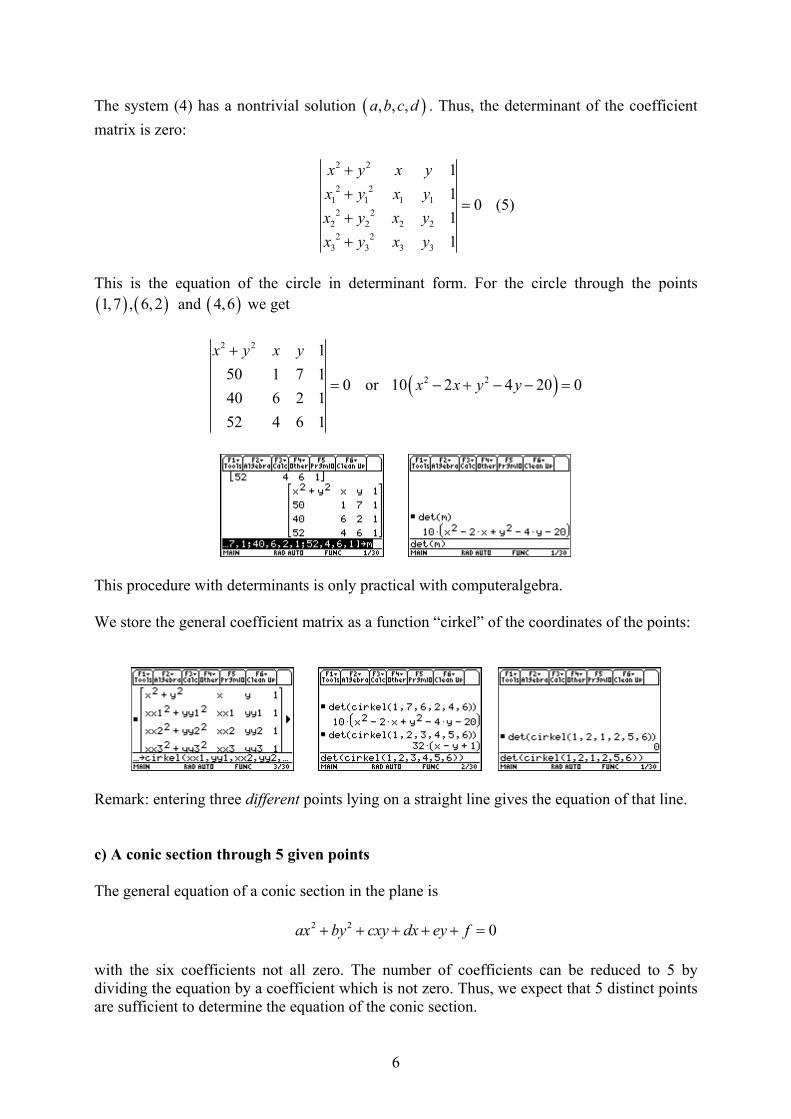
This is the equation of the circle in determinant form. For the circle through the points ( ) ( )1,7 , 6, 2 and ( )4,6 we get

2 2 150 1 7 1

040 6 2 152 4 6 1

x y x y+

= or ( )2 210 2 4 20 0x x y y− + − − =

This procedure with determinants is only practical with computeralgebra. We store the general coefficient matrix as a function “cirkel” of the coordinates of the points:

Remark: entering three different points lying on a straight line gives the equation of that line. c) A conic section through 5 given points The general equation of a conic section in the plane is

2 2 0ax by cxy dx ey f+ + + + + = with the six coefficients not all zero. The number of coefficients can be reduced to 5 by dividing the equation by a coefficient which is not zero. Thus, we expect that 5 distinct points are sufficient to determine the equation of the conic section.

7

Analogous with the last section we find the equation in determinant form:

2 2

2 21 1 1 1 1 1

2 22 2 2 2 2 2

2 23 3 3 3 3 3

2 24 4 4 4 4 4

2 25 5 5 5 5 5

111

0111

x y xy x yx y x y x yx y x y x yx y x y x yx y x y x yx y x y x y

=

As an illustration we determine the equation of the conic section through the points ( ) ( ) ( ) ( ) ( )1, 2 , 2,3 , 4,6 , 5, 2 , 3, 4− − − . The result is 2 2228 163 517 1946 1833 4154 0x y xy x y− − + + − = (after division by 36).

Because 228 517 / 2

0517 / 2 163

−<

− − , the conic section is a hyperbola.

The general coefficient matrix is stored as the function “ks” of the coordinates of the points:

The conic section through the points ( ) ( ) ( ) ( ) ( )1,1 , 1,1 , 1, 1 , 1, 1 , 0,0− − − − is 2 2 0x y− = , a pair of lines (degenerated conic).

8

d) The ellipse as a locus of points An ellipse is the set of points ( ),x y such that the sum of the distances from ( ),x y to two given points (the foci) is fixed. Choose an orthonormal axis system. Let ( ),x y=p be a general point of the ellipse and

( ),f fx y=f , ( ),g gx y=g the foci, then we have:

( ) ( ), , 2d d a+ =p f p g (6) The triangle inequality gives

( ) ( ) ( ), , + ,d d d≤f g f p p g or ( ), 2d a≤f g (7).

We demand the strict inequality ( ), 2d a<f g because ( ), 2d a=f g results in the segment connecting f with g .

The distance formula gives ( ) ( ) ( )2 2, f fd x x y y= − = − + −p f p f

Our goal is to get rid of the square roots associated with (6): squaring ( ) ( ), 2 ,d a d= −p f p g yields

( ) ( ) ( )2 22, 4 4 , ,d a a d d= − ⋅ +p f p g p g or ( ) ( ) ( )2 224 , 4 , ,a d a d d⋅ = + −p g p g p f

squaring again gives ( ) ( ) ( )( )22 2 22 216 , 4 , , 0a d a d d⋅ − + − =p g p g p f (8)

The expression (8) is “simplified” with computeralgebra, resulting in the equation of the ellipse. The left-hand side of that equation is stored as the function ( )ellips , , , ,xf yf xg yg a , with as variables the coordinates of the foci and the length a of the half major axis. This is a long expression (see the fourth screen shot below).

9

As an example, the equation ( )ellips 4,0, 4,0,5 0− = of the ellipse with the foci (4,0) ,

( )4,0− and 5a = yields 2 2144 400 3600 0x y+ − = or 2 2

2 2 15 3x y

+ = .

( )ellips ,0, ,0, 0c c a− = becomes ( )2 2 2 2 2 4 2 216 16 16 16 16 0a c x a y a a c− + − + =

or ( ) ( )2 2 2 2 2 2 2 2a c x a y a a c− + = −

with 2 2 2b a c= − , this gives the standard equation 2 2

2 2 1x ya b

+ = .

De choice of the foci is free;

( )ellips 5, 2, 4, 2,8 0− − = becomes 2 2700 288 960 700 144 40529 0x xy y x y− + − + − = :

Remark: We tend to choose a value a with ( ), 2d a>f g , such that the triangle inequality (7) is not satisfied. Exploring with ( )ellips 5,0, 5,0, 4 0− = gives 2 2144 256 2304 0x y− + + = or the hyperbola

2 2

116 9x y

− = !!

10

One can check that also a hyperbola with ( ) ( ), , 2d d a− =p f p g and ( ), 2d a>f g satisfies the equation (8)! (Hint: ( ) ( ), , 2d d a− =p f p g is equivalent with ( ) ( ), 2 ,d a d= ± +p f p g ) Thus, the function ( )ellips , , , ,xf yf xg yg a results in an ellipse or a hyperbola with given foci

( ),f fx y=f en ( ),g gx y=g , depending on whether the distance between f en g is less than or greater than 2a . 4.3 Eigenvalues and eigenvectors The problem of finding a number λ and a vector ≠x 0 such that A λ=x x has a lot of applications. a) The Cayley-Hamilton theorem The Cayley-Hamilton theorem can be introduced as:

• choose a 2 2× matrix A and find its characteristic polynomial ( ) ( )detp A Iλ λ= −

• replace λ in ( )p λ by A (with this 0λ is replaced by 0A I= ) • what is the result? Try also with a 3 3× and a 4 4× matrix.

We always obtain the zero matrix and suspect in general that each matrix A satisfies its own characteristic equation: if ( ) 0p λ = is the characteristic equation A, then ( ) 0p A = (the zero matrix). This is the Cayley-Hamilton theorem.

For 4 4

0 3A

− =

the characteristic equation becomes 2 12 0λ λ+ − = so that

11

2 12 0A A I+ − = or 2 12A I A= − . Thus 3A can also be expressed in terms of A and I:

( ) ( )3 2 212 12 12 1213 12

A A A I A A A A A I AA I

= = − = − = − −

= −

For any natural number 2k ≥ , the matrix kA can be written as kA A Iα β= + , where α and β are constants whose values will depend on k. b) The Gerschgorin circles Let ijA a = be a square matrix of order n, then every eigenvalue of A lies inside (or on) at

least one of the circles (called Gerschgorin circles) in the complex plane with center iia and

radii , ,1, 1

n n

i i j i j iij j i j

r a a a= ≠ =

= = −

∑ ∑ ( 1,2,3, )i n= K .

Thus all the eigenvalues of A lie in the union of the discs

{ }:i ii iD z C z a r= ∈ − ≤ ( 1,2,3, )i n= K . This first Gerschgorin theorem provides a quick graphic view of the position of the eigenvalues.

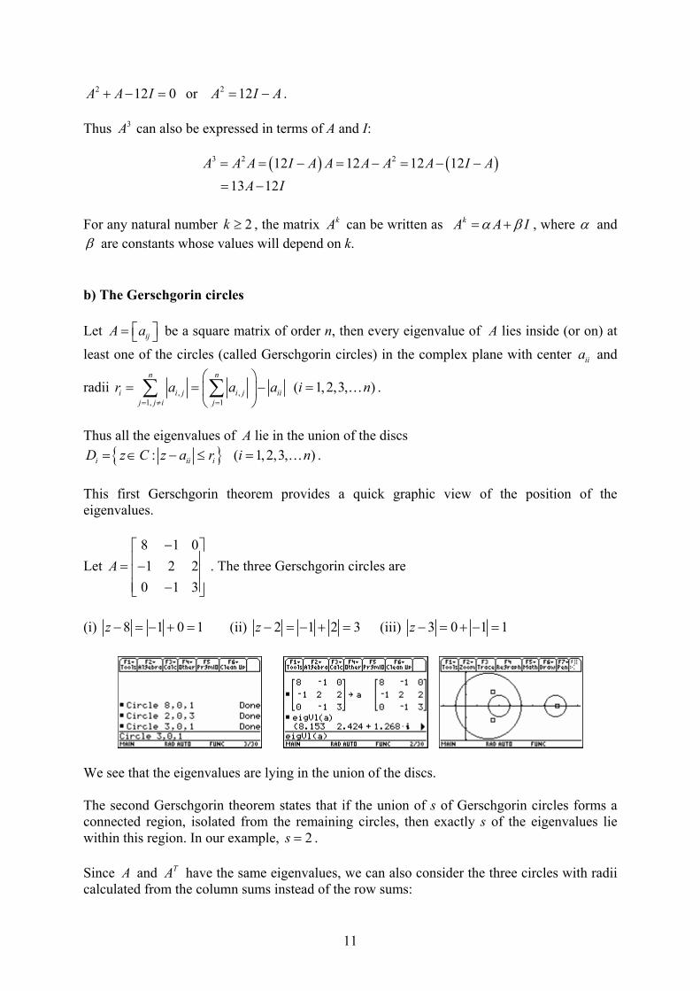
Let 8 1 01 2 2

0 1 3A

− = − −

. The three Gerschgorin circles are

(i) 8 1 0 1z − = − + = (ii) 2 1 2 3z − = − + = (iii) 3 0 1 1z − = + − =

We see that the eigenvalues are lying in the union of the discs. The second Gerschgorin theorem states that if the union of s of Gerschgorin circles forms a connected region, isolated from the remaining circles, then exactly s of the eigenvalues lie within this region. In our example, 2s = . Since A and TA have the same eigenvalues, we can also consider the three circles with radii calculated from the column sums instead of the row sums:

12

The eigenvalues lie in the intersection of the two unions of three discs. Applications:

• If the origin doesn’t lie in the union of the discs associated with the matrix A, then 0 is not an eigenvalue of A. This means that A has an inverse.

• A system A′ =u u of linear first order differential equations, with A diagonalizable, is

stable if all the eigenvalues of A have a strict negative real part. This is certainly the case if all the circles of Gerschgorin are lying in the half plane 0x < .

• All the eigenvalues are lying in the disc ( )1

max 1, 2,n

iji jz a i n

=

≤ =

∑ K (analogous

for the column sums).

c) Markov chains Suppose that the annual population migration between three geographical regions A, B and C is given by the following transition diagram.

For example, 10% of the population in region A moves annually to region C. This transition is governed by the following transition matrix:

A B

C

0.8 0.2

0.2

0.1

0.10.3

0.5

0.2 0.6

13

from :to :

0.8 0.3 0.20.1 0.2 0.60.1 0.5 0.2

A B CA

P BC

=

This matrix in a stochastic matrix (the column sums add up to 1). 1) Suppose that the initial distribution (our first observation) of the population is given by the

initial state vector 0

0.40.50.1

=

x (i.e. a probability vector with nonnegative entries that add

up to 1). At that moment, 40% of the population lives in A, 50% in B and 10% in C. The Markov chain is a sequence of state vectors 0 1 0 2 1 3 2, , , ,P P P= = =x x x x x x x K ( kx is the state vector after k years). This leads to 1k kP+ =x x or 0

kk P=x x for 0,1, 2,k = K

Calculate the successive state vectors and study the long-run population distribution. Then choose another initial state vector 0x and observe the long run distribution. Conjecture? 2) Find a steady-state vector (or equilibrium vector) for P, i.e. a probability vector q such that P =q q . Conjecture? 3) Observe the evolution of kP for 1, 2,k = K . Conjecture? The calculator can do the calculations: 1)

14

The state vectors converge to 0.5570.2300.213

, independent of the initial distribution (choose

another 0x and see what happens)! 2) Remark that P =q q certainly has a solution as a stochastic matrix P always has

eigenvalue 1 ( for TP the vector 111

is an eigenvector with eigenvalue 1).

All the eigenvalues are lying in the disc ( )1

max 1, 2,3n

ijj i

z a j=

≤ = ∑ or 1z ≤ .

The eigenspace corresponding to the eigenvalue 1 is given by

1

2 3

3

34 /1314 /13

1

xx xx

=

with 3x R∈ . For 3 13x = we find the eigenvector 341413

, dividing

by 34 14 13 61+ + = gives the only steady state vector 34 / 6114 / 6113/ 61

=

q with P =q q .

The Markov chain 0 1 2 3, , , ,x x x x K seems to converge to q , independent of the initial state vector 0x . Can we prove this conjecture?

15

Choose a basis { }1 2 3, ,v v v for 3R , existing of eigenvectors of P with corresponding

eigenvalues 1 1λ = , 2 0.55λ = , 3 0.35λ = − . Let 1

341413

=

v .

The vector 0x can be written as a unique linear combination of the basis vectors: 0 1 1 2 2 3 3c c c= + +x v v v Then 1 0 1 1 2 2 3 3 1 1 2 2 3 30.55 ( 0.35)P c P c P c P c c c= = + + = + + −x x v v v v v v

and ( ) ( )2 22 1 1 1 2 2 3 3 1 1 2 2 3 30.55 ( 0.35) 0.55 0.35P c P c P c P c c c= = + + − = + + −x x v v v v v v

in general we find: ( ) ( )1 1 2 2 3 30.55 0.35k k

k c c c= + + −x v v v for 1, 2,k = K . We conclude that 1 1lim kk

c→∞

=x v

The limiting vector belongs to the eigenspace of P corresponding to 1λ = . Every kx is a probability vector with column sum 1, therefore the limiting vector must be a probability vector too.

1 1 1

341413

c c =

v with 1 1 134 14 13 1c c c+ + = , thus 1 1/ 61c = and 1 1

34 / 6114 / 6113/ 61

c = =

v q .

The result is independent of the initial state vector 0 1 1 2 2 3 3c c c= + +x v v v . Observe that the first term 1 1c =v q is the same for every initial state vector! 3) We observe successive powers of the transition matrix P:

16

We suspect that [ ]lim k

kP

→∞= q q q

Can we prove this conjecture? Remark that [ ]1 2 3

1 2 3

k k k

k k k

P P I P

P P P

= ⋅ = ⋅

=

e e e

e e e

[ ]1 2 3lim lim lim limk k k k

k k k kP P P P

→∞ →∞ →∞ →∞ = = e e e q q q

since 1 2 3, ,e e e are probability vectors. Theorem: If P is an n n× regular stochastic matrix (i.e. there exists a k such that kP contains only strictly positive elements), then P has a unique steady state vector q (i.e. P =q q ). Moreover, if 0x is any initial state vector and 1k kP+ =x x for 0,1, 2,k = K , than the Markov chain { }kx converges to q and kP to [ ]q q qK as k →∞ . d) Diagonalization of a square matrix An n n× matrix A is diagonalizable if A is similar to a diagonal matrix, that is, if 1A PDP−= for some invertible matrix P and some diagonal matrix D. The columns of P are n linearly independent eigenvectors of A and the diagonal entries D are the successive corresponding eigenvalues of A. Diagonalization occurs in

• Diagonalizing quadatric forms. • Linear discrete and linear continuous dynamical systems (systems of linear first-order

difference equations or differential equations). • The calculation of matrixfunctions.

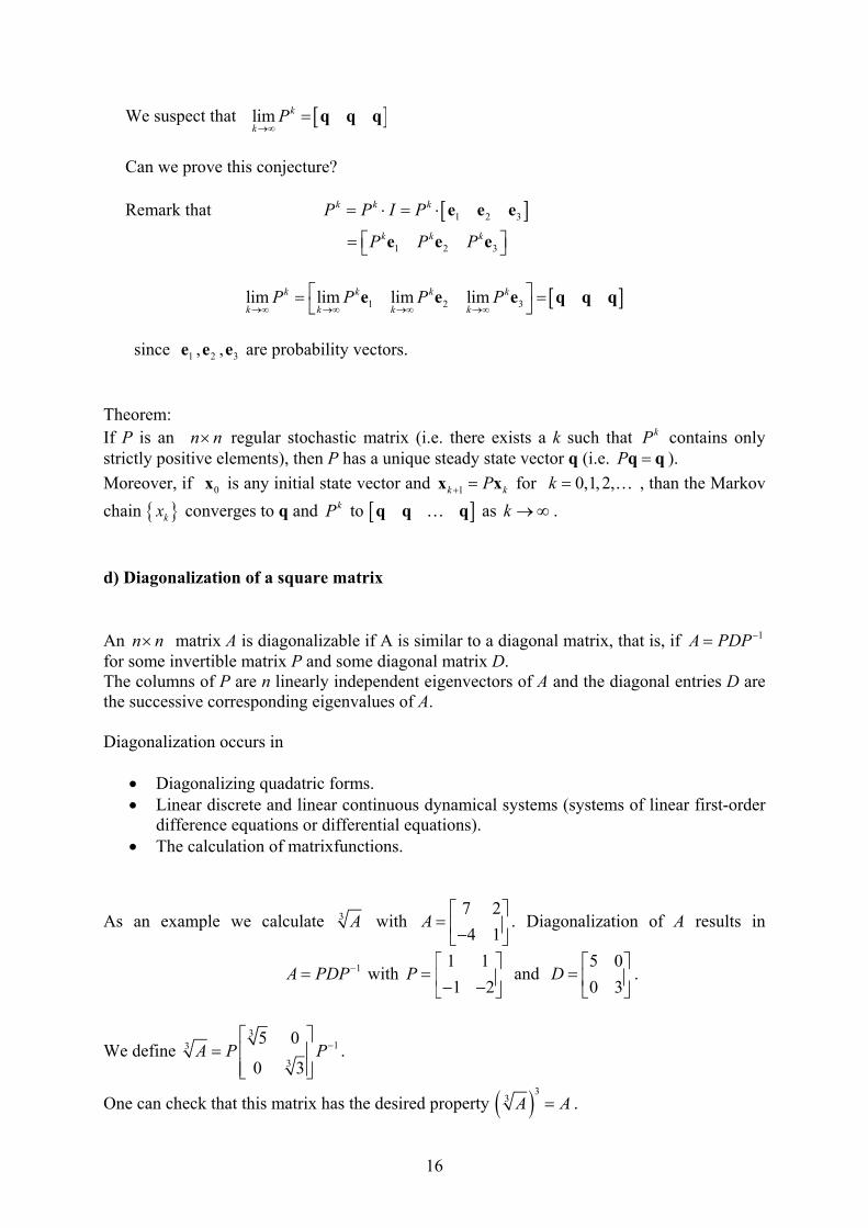
As an example we calculate 3 A with 7 24 1

A = −

. Diagonalization of A results in

1A PDP−= with 1 11 2

P = − −

and 5 00 3

D =

.

We define 3

13

3

5 0

0 3A P P−

=

.

One can check that this matrix has the desired property ( )33 A A= .

17

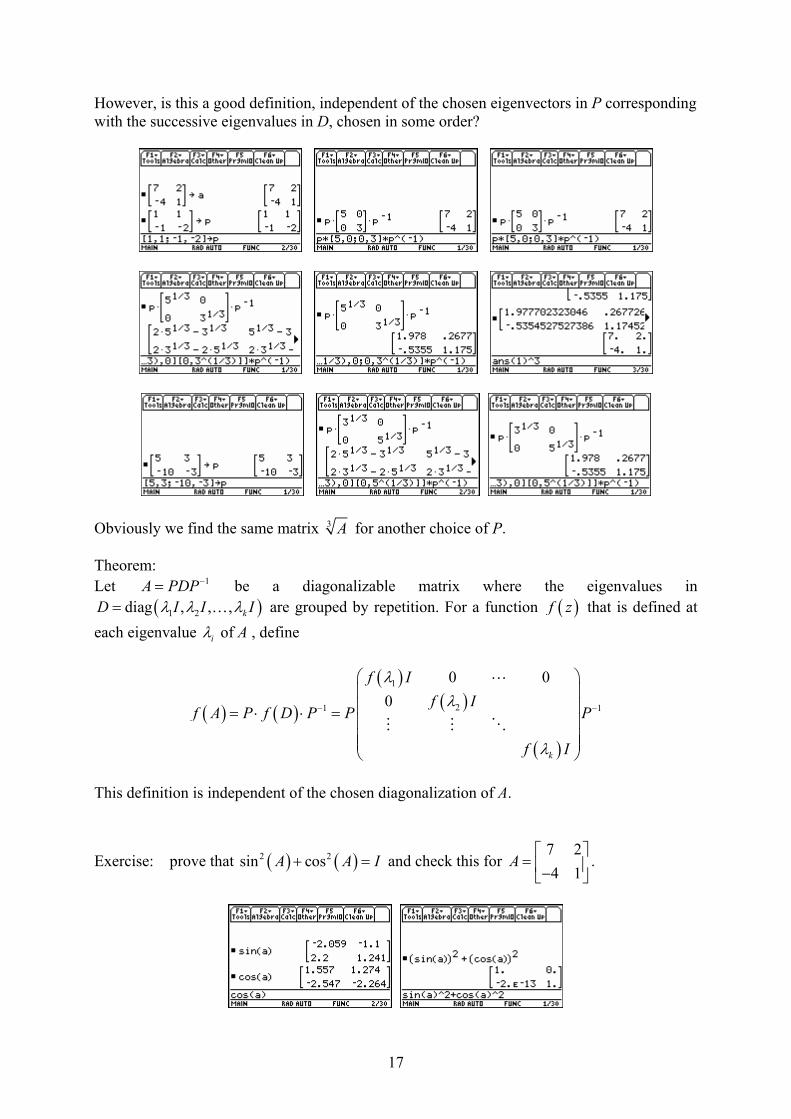
However, is this a good definition, independent of the chosen eigenvectors in P corresponding with the successive eigenvalues in D, chosen in some order?

Obviously we find the same matrix 3 A for another choice of P. Theorem: Let 1A PDP−= be a diagonalizable matrix where the eigenvalues in

( )1 2diag , , , kD I I Iλ λ λ= K are grouped by repetition. For a function ( )f z that is defined at each eigenvalue iλ of A , define

( ) ( )

( )( )

( )

1

21 1

0 00

k

f If I

f A P f D P P P

f I

λλ

λ

− −

= ⋅ ⋅ =

L

M M O

This definition is independent of the chosen diagonalization of A.

Exercise: prove that ( ) ( )2 2sin cosA A I+ = and check this for 7 24 1

A = −

.

18

e) Exploring eigenvalues of matrices 1) Let the TI-89 generate two 3 3× matrices A and B with integer values between -9 and 9. Find the eigenvalues of A and B. i) Find the eigenvalues of A B+ . Conjecture? ii) Find the eigenvalues of AB . Conjecture? iii) Find the eigenvalues of 5A and 3B . Conjecture? iii) Compare the eigenvalues of AB and BA. Conjecture?

2) Construct a 3 3× matrix A (not diagonal or triangular) with integer entries and eigenvalues 1, 1 and 2. Solution: It suffices to find a matrix P with integer entries and ( )det 1P = . Then the matrix ( ) 1diag 1,1,2A P P−= ⋅ ⋅ has the desired properties. Let TP L L= ⋅ where L is a lower triangular matrix with integer entries and 1’s on the diagonal.

19

4.4 Orthogonality and least-squares problems a) Orthogonal bases for a vector space simplify the calculations, they play an important role in numerical analysis, such as the “QR factorization” where an m n× matrix A with linearly independent columns is factored as A QR= (where Q is an m n× matrix whose columns form an orthonormal basis for the column space of A, and R is an n n× invertible upper triangular matrix with positive entries on its diagonal).

b) Orthogonal projections are the key for finding “solutions” for overdetermined systems. In practice, systems of linear equations with more equations than unknowns and no solutions often appear. For example, how can we find the “best” line y ax b= + “through” ( ) ( ) ( ) ( )0,0 , 1,1 , 2, 2 , 3, 2 ? We desire that i iy ax b= + ( )1, 2,3, 4i = but this system

0 01

2 23 2

a ba b

a ba b

+ = + = + = + =

or

0 1 01 1 12 1 23 1 2

a b

+ =

or

0 1 01 1 12 1 23 1 2

ab

=

or A =x y

has no solution x. A “best” solution x̂ gives a vector ˆAx as close as possible to y , in the sense that ( )ˆ ˆ,d A A A= − ≤ −x y x y x y for each 2R∈x .

We call x̂ a least-squares solution, the corresponding least-squares line minimizes the sum of the squares of the vertical deviations of the given points to the line. The vector ˆAx belongs to the column space of A (notation Col A ). The closest vector in Col A to y is the orthogonal projection of y onto Col A, this is the unique vector Colproj A y where Colproj A= +y n y and olC A⊥n .

20

Such a vector x̂ where Colˆ proj AA =x y surely exists because if x runs over 2R , then Ax runs over the complete column space of A. We demand that ˆA= +y n x and olC A⊥n or ˆ olA C A− ⊥y x . The columns of A generate Col A . Thus, the vector ˆA−y x is orthogonal to Col A if and only if ˆA−y x is orthogonal to the column vectors of [ ]1 2A = a a . This means that ( )1 ˆ 0T A− =a y x and ( )2 ˆ 0T A− =a y x or ( )ˆTA A− =y x 0 . Consequently, ˆT TA A A=x y (the system of normal equations). A least-squares solution x̂ of A =x y can be found by solving the system ˆT TA A A=x y . The matrix TA A is invertible if and only if the columns of A are linearly independent (as in our example), in that case we find the unique solution ( ) 1

ˆ T TA A A−

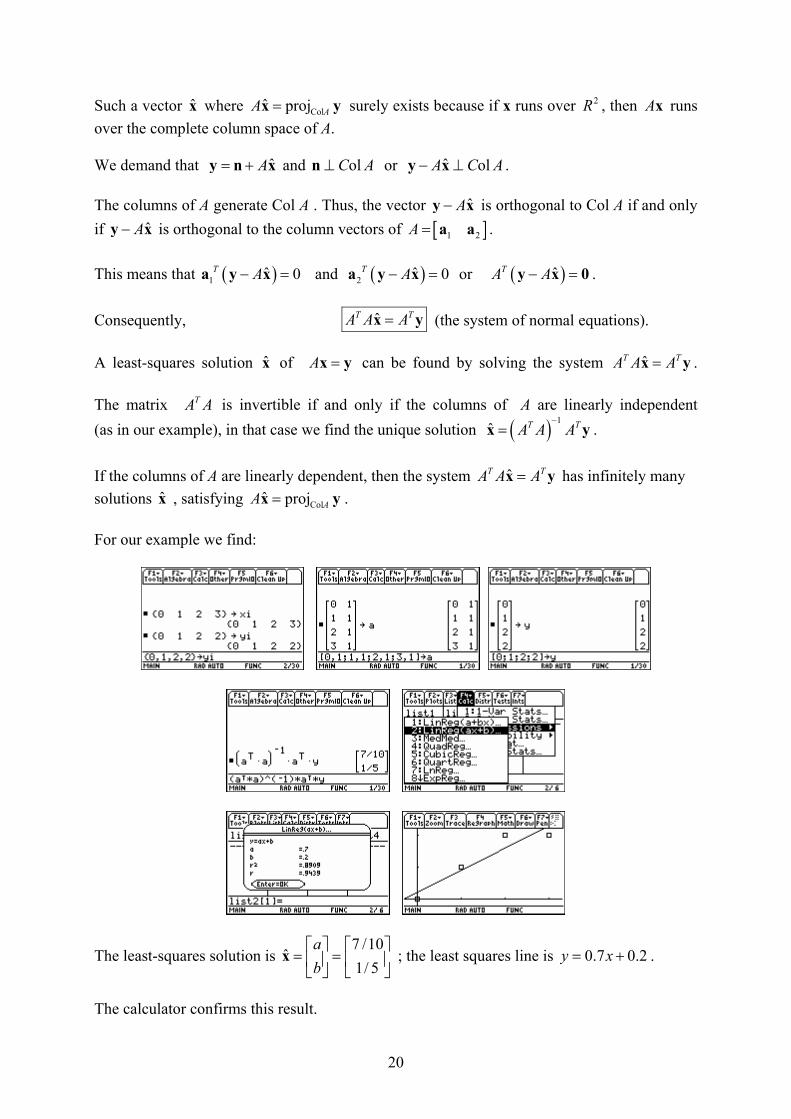
=x y . If the columns of A are linearly dependent, then the system ˆT TA A A=x y has infinitely many solutions x̂ , satisfying Colˆ proj AA =x y . For our example we find:

The least-squares solution is 7 /10

ˆ1/ 5

ab

= =

x ; the least squares line is 0.7 0.2y x= + .

The calculator confirms this result.

21

5 Conclusion With the foregoing examples we have illustrated that the TI-89 can help to

• get the correct answer quickly, • explore methods that are too time-consuming with manual calculations, • gain insight in introducing new mathematical concepts, • explore different situations, leading to conjectures • draw graphical representations.

6 Sources 1. H. Anton, C. Rorres, Elementary Linear Algebra, Applications Version, John Wiley & Sons, 1991. 2. S.I. Grossman, Elementary Linear Algebra, fourth edition, Saunders College Publishing, 1991. 3. G. James, Advanced Modern Engineering mathematics, third edition, Pearson Education, 2004. 4. D.C. Lay, Linear Algebra and Its Applications, third edition update, Pearson Education, 2006. 5. C.D. Meyer, Matrix Analysis and Applied Linear Algebra, Siam, 2000.