Applied Econometrics

Lecture 15:

Sample Selection Bias

Estimation of Nonlinear Models with Panel Data

Måns Söderbom�

13 October 2009

�University of Gothenburg. Email: mans:soderbom@economics:gu:se. Web: http://www.soderbom.net

1. Introduction

In this the last lecture of the course we discuss two topics: How to estimate regressions if your sample

is not random, in which case there may be sample selection bias; and how to estimate nonlinear models

(focussing mostly on probit) if you have panel data.

References sample selection:

� Wooldridge (2002) Chapter 17.1-17.2; 17.4 (read carefully)

� Vella, Francis (1998), "Estimating Models with Sample Selection Bias: A Survey," Journal of

Human Resources, 33, pp. 127-169 (optional)

� François Bourguignon, Martin Fournier, Marc Gurgand"Selection Bias Corrections Based on the

Multinomial Logit Model: Monte-Carlo Comparisons" DELTA working paper 2004-20, download-

able at http://www.delta.ens.fr/abstracts/wp200420.pdf (useful background reading for computer

exercise 5)

References panel data models:

� Wooldridge (2002), Chapters 15.8.1-3; 16.8.1-2; 17.7 (read carefully).

2. Sample Selection

� Up to this point we have assumed the availability of a random sample from the underlying pop-

ulation. In practice, however, samples may not be random. In particular, samples are sometimes

truncated by economic variables.

� We write our equation of interest (sometimes referred to as the �structural equation�or the �primary

equation�) as

y1 = x1�1 + u1; (2.1)

1

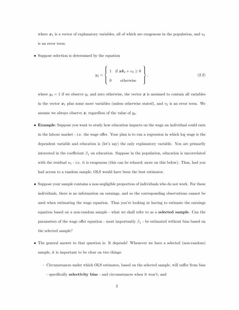
where x1 is a vector of explanatory variables, all of which are exogenous in the population, and u1

is an error term.

� Suppose selection is determined by the equation

y2 =

8>><>>:1 if x�2 + v2 � 0

0 otherwise

9>>=>>; ; (2.2)

where y2 = 1 if we observe y1 and zero otherwise, the vector x is assumed to contain all variables

in the vector x1 plus some more variables (unless otherwise stated), and v2 is an error term. We

assume we always observe x, regardless of the value of y2.

� Example: Suppose you want to study how education impacts on the wage an individual could earn

in the labour market - i.e. the wage o¤er. Your plan is to run a regression in which log wage is the

dependent variable and education is (let�s say) the only explanatory variable. You are primarily

interested in the coe¢ cient �1 on education. Suppose in the population, education is uncorrelated

with the residual u1 - i.e. it is exogenous (this can be relaxed; more on this below). Thus, had you

had access to a random sample, OLS would have been the best estimator.

� Suppose your sample contains a non-negligible proportion of individuals who do not work. For these

individuals, there is no information on earnings, and so the corresponding observations cannot be

used when estimating the wage equation. Thus you�re looking at having to estimate the earnings

equation based on a non-random sample - what we shall refer to as a selected sample. Can the

parameters of the wage o¤er equation - most importantly �1 - be estimated without bias based on

the selected sample?

� The general answer to that question is: It depends! Whenever we have a selected (non-random)

sample, it is important to be clear on two things:

�Circumstances under which OLS estimates, based on the selected sample, will su¤er from bias

- speci�cally selectivity bias - and circumstances when it won�t; and

2

� If there is selectivity bias in the OLS estimates: how to obtain estimates that are not biased

by sample selection.

2.1. When will there be selection bias, and what can be done about it?

� I will now discuss estimation of the model above under the following assumptions:

� Assumption 17.1 (Wooldridge, p.562):

� (a) (x;y2) are always observed, but y1 is only observed when y2 = 1 (sample selection);

� (b) (u1; v2) is independent of x with zero mean (x is exogenous in the population);

� (c) v2~Normal (0; 1) (distributional assumption); and

� (d) E (u1jv2) = 2v2 (residuals may be correlated; e.g. bivariate normality).

� Note that, given var (v2) = 1, 2 measures the covariance between u1 and v2.

� The fundamental issue to consider when worrying about sample selection bias is why some indi-

viduals will not be included in the sample. As we shall see, sample selection bias can be viewed as

a special case of endogeneity bias, arising when the selection process generates endogeneity in

the selected sub-sample.

� In our model, and given assumption 17.1, sample selection bias arises when the residual in the

selection equation (i.e. v2) is correlated with the residual in the primary equation (i.e. u1), i.e.

whenever 2 6= 0. To see this, we will derive the expression for E (y1jx; y2 = 1), i.e. the expectation

of the outcome variable conditional on observable x and selection into the sample.

� We begin by deriving E (y1jx; v2):

E (y1jx; v2) = x1�1 + E (u1jx; v2)

= x1�1 + E (u1jv2)

E (y1jx; v2) = x1�1 + 1v2: (2.3)

3

Part (b) of Assumption 17.1 (independence between x and u1) enables us to go from the �rst to

the second line; part (d) enables us to go from the second to the third line.

� Since v2 is not observable, eq (2.3) is not directly usable in applied work (since we can�t condition

on unobservables when running a regression). To obtain an expression for the expected value of

y1 conditional on observables x and the actual selection outcome y2, we make use of the law of

iterated expectations (see e.g. Wooldridge, p.19):

E (y1jx; y2) = E [E (y1jx; v2) jx; y2] :

Hence, using (2.3) we obtain

E (y1jx; y2) = E [(x1�1 + 1v2) jx; v2; y2] ;

E (y1jx; y2) = x1�1 + 1E (v2jx; y2) ;

E (y1jx; y2) = x1�1 + 1h (x; y2) ;

where h (x; y2) = E (v2jx; y2) is some function (note that, since we condition on x and y2 it is not

necessary to condition on v2, hence the latter term vanishes when we go from the �rst to the second

line).

� Because the selected sample has y2 = 1, we only need to �nd h (x; 1). Our model and assumptions

imply

E (v2jx; y2 = 1) = E (v2jv2 � �x�2) ;

and so we can use our �useful result�appealed to in the previous lecture:

E (zjz > c) =� (c)

1� � (c) ; (2.4)

where z follows a standard normal distribution, c is a constant, � denotes the standard normal

4

probability density function, and � is the standard normal cumulative density function. Thus

E (v2jv2 � �x�2) =� (�x�2)

1� � (�x�2)

E (v2jv2 � �x�2) =� (x�2)

� (x�2)� � (x�2) ;

where � (�) is the inverse Mills ratio (see Section 1 in the appendix for a derivation of the inverse

Mills ratio). We now have a fully parametric expression for the expected value of y1; conditional

on observable variables x, and selection into the sample (y2 = 1):

E (y1jx; y2 = 1) = x1�1 + 1� (x�2) .

2.1.1. Exogenous sample selection: E (u1j v2) = 0

� Assume that the unobservables determining selection are independent of the unobservables deter-

mining the outcome variable of interest:

E (u1j v2) = 0:

In this case, we say that sample selection is exogenous, and - here�s the good news - we can

estimate the main equation of interest by means of OLS, since

E (y1jx; y2 = 1) = x1�1;

hence

y1 = x1�1 + &i;

where &i is a mean-zero residual that is uncorrelated with x1 in the selected sample (recall we

assume exogeneity in the population). Examples:

5

� Suppose sample selection is randomized (or as good as randomized). Imagine an urn containing

a lots of balls, where 20% of the balls are red and 80% are black, and imagine participation in

the sample depends on the draw from this urn: black ball, and you�re in; red ball and you�re

not. In this case sample selection is independent of all other (observable and unobservable)

factors (indeed �2 = 0). Sample selection is thus exogenous.

� Suppose the variables in the x-vector a¤ect the likelihood of selection (i.e. �2 6= 0). Hence

individuals with certain observable characteristics are more likely to be included in the sample

than others. Still, we�ve assumed x to be independent of the residual in the main equation,

u1, and so sample selection remains exogenous. In this case also - no problem.

2.1.2. Endogenous sample selection: E (u1j v2) 6= 0

Sample selection results in bias if the unobservables u1 and v2 are correlated, i.e. 1 6= 0. Recall:

E (y1jx; y2 = 1) = x1�1 + 1� (x�2)

� This equation tells us that the expected value of yi, given x and observability of y1 (i.e. y2 = 1)

is equal to xi�, plus an additional term that depends on the inverse Mills ratio evaluated at zi .

Hence in the selected sample, actual y1 is written as the sum of expected y1 (conditional on x and

selection) and a mean-zero residual:

y1 = x1�1 + 1� (x�2) + &i,

� It follows that if, based on the selected sample, we use OLS to run a regression in which y1 is the

dependent variable and x1 is the set of explanatory variables, then � (x�2) will go into the residual;

and to the extent that � (x�2) is correlated with x1, the resulting estimates will be biased unless

1 = 0.

6

2.1.3. An example

Based on these insights, let�s now think about estimating the following simple wage equation based on a

selected sample.

lnwi = �0 + �1educi + "i;

� Always when worrying about endogeneity, you need to be clear on the underlying mechanisms. So

begin by asking yourself: What factors are likely to go into the residual "i in the wage equation?

Clearly individuals with the same levels of education can obtain very di¤erent wages in the labour

market, and given how we have written the model it follows by de�nition that the residual "i is the

source of such wage di¤erences. To keep the example simple, suppose I�ve convinced myself that

the (true) residual "i consists of two parts:

"i = �1mi + ei;

where mi is personal �motivation�, which is unobserved (note!) and assumed uncorrelated with

education in the population (clearly a debatable assumption, but let�s keep it simple), �1 is a positive

parameter, and ei re�ects the remaining source of variation in wages. Suppose for simplicity that

ei is independent of all variables except wages.

� I know from my econometrics textbook that there will be sample selection bias in the OLS estimator

if the residual in the earnings equation "i is correlated with the residual in the selection equation.

Let�s now relate this insight to economics, sticking to our example. Since motivation (mi) is

(assumed) the only economically interesting part of "i; I thus need to ask myself: Is it reasonable

to assume that motivation is uncorrelated with education in the selected sample? For now,

maintain the assumption that motivation and education are uncorrelated in the population - hence

had there been no sample selection, education would have been exogenous and OLS would have

been �ne.

7

� Still - and this is the key point - I may suspect that selection into the labour market depends on

education and motivation:

y2i =

8>><>>:1 if � educi + (�2mi + �i) � 0

0 otherwise

9>>=>>; ;

where �2 is a positive parameter and �i is a residual independent of all factors except selection.

Because mi is unobserved it will go into the residual, which will consist of the two terms inside the

parentheses (:).

� The big question now is whether the factors determining selection are correlated with the wage

residual "i = �1mi + ei. There are only three terms determining selection. Two of these are

�i and educi; and they have been assumed uncorrelated with "i. But what about motivation,

mi? Abstracting from the uninteresting case where �1 and/or �2 are equal to zero, we see that

i) motivation determines selection; and ii) motivation is correlated with the wage residual since

"i = �1mi + ei. So clearly we have endogenous selection.

� Does this imply that education is correlated with "i in the selected sample? Yes it does. The

intuition as to why this is so is straightforward. Think about the characteristics (education and

motivation) of the people that are included in the sample.

� Someone with a low level of education must have a high level of motivation, otherwise he

or she is likely not to be included in the sample (recall: the selection model implies that

individuals with low levels of education and low levels of motivation are those most unlikely

to be included in the sample).

� In contrast, someone with a high level of education is fairly likely to participate in the labour

market even if he or she happens to have a relatively low level of motivation.

� The implication is that, in the sample, the average level of motivation among those with little

education will be higher than the average level of motivation with those with a lot of education. In

8

other words, education and motivation are negatively correlated in the sample, even though this

is not the case in the population.

� And since motivation goes into the residual (since we have no data on motivation - it�s unobserved),

it follows that education is (negatively) correlated with the residual in the selected sample. And

that�s why we get selectivity bias.

� Illustration: Figure 2 in the appendix.

2.2. How correct for sample selection bias?

I will now discuss the two most common ways of correcting for sample selection bias.

2.2.1. Method 1: Inclusion of control variables

The �rst method by which we can correct for selection bias is simple: include in the regression observed

variables that control for sample selection. In the wage example above , if we had data on motivation,

we could just augment the wage model with this variable:

lnwi = �0 + �1educi + �1mi + ei:

More generally, recall that

E (y1jx; v2) = x1�1 + 1v2:

and so if you have data on v2, we could just use include this variable in the model as a control variable

for selection and estimate the primary equation using OLS. Such a strategy would completely solve the

sample selection problem.

Clearly this approach is only feasible if we have data on the relevant factors (e.g. motivation), which

may not always be the case. The second way of correcting for selectivity bias is to use the famous Heckit

method, developed by James Heckman in the 1970s.

9

2.2.2. Method 2: The Heckit method

We saw above that

E (y1jx; y2 = 1) = x1�1 + 1� (x�2) :

Using the same line of reasoning as for �Method 1�, it must be that if we had data on � (x�2), we could

simply add this variable to the model and estimate by OLS. Such an approach would be �ne. Of course,

in practice you would never have direct data on � (x�2). However, the functional form � (�) is known

and x is (it is assumed) observed. If so, the only missing piece is the parameter vector �2, which can be

estimated by means of a probit model. The Heckit method thus consists of the following two steps:

1. Using all observations - those for which y2 is observed (selected observations) and those for which

it is not - and estimate a probit model where y2 is the dependent variable and x are the explana-

tory variables. Based on the parameter estimates �̂2, calculate the inverse Mills ratio for each

observation:

��x�̂2

�=��x�̂2

���x�̂2

� :2. Using the selected sample, i.e. all observations for which y2 is observed, and run an OLS regression

in which y2 is the dependent variable and x1 and ��x�̂2

�are the explanatory variables:

y1 = x1�1 + 1��x�̂2

�+ &i.

This will give consistent estimates of the parameter vector �1. That is, by including the inverse

Mills ratio as an additional explanatory variable, we have corrected for sample selectivity.

Important considerations

� The Heckit procedure gives you an estimate of the parameter 1, which measures the covariance

between the two residuals u1 and v2. Under the null hypothesis that there is no selectivity bias, we

have 1 = 0. Hence testing H0 : 1 = 0 is of interest, and we can do this by means of a conventional

10

t-test. If you cannot reject H0 : 1 = 0 then this indicates that sample selection does not result

in signi�cant bias, and so using OLS on the selected sample without including the inverse Mills

ratio is �ne - all this, under the assumption that the model is correctly speci�ed and that (a)-(d)

in Assumption 17.1 hold, of course.

� We assumed above that the vector x (the determinants of selection) contains all variables that go

into the vector x1 (the explanatory variables in the primary equation), and possibly additional

variables. In fact, it is highly desirable to specify the selection equation in such a way that there

is at least one variable that determines selection, and which has no direct e¤ect on yi. In other

words, it is important to impose at least one exclusion restriction. The reason is that if x1 = x, the

second stage of Heckit is likely to su¤er from a collinearity problem, with very imprecise estimates

as a result. Recall the form of the regression you run in the second stage of Heckit:

y1 = x1�1 + 1��x�̂2

�+ &i.

Clearly, if x1 = x, then

y1 = x1�1 + 1��x1�̂2

�+ &i:

Remember that collinearity arises when one explanatory variable can be expressed as a linear

function of one or several of the other explanatory variables in the model. In the above model

x1 enters linearly (the �rst term) and non-linearly (through inverse Mills ratio), which seems to

suggest that there will not be perfect collinearity. However, if you look at the graph of the inverse

Mills ratio (see Figure 1 in the appendix) you see that it is virtually linear over a wide range

of values. Clearly had it been exactly linear there would be no way of estimating

y1 = x1�1 + 1��x1�̂2

�+ &i:

because x1 would then be perfectly collinear with ��x1�̂2

�. The fact that Mills ratio is virtually

11

linear over a wide range of values means that you can run into problems posed by severe (albeit not

complete) collinearity. This problem is solved (or at least mitigated) if x contains one or several

variables that are not included in x1.

� Finally, always remember that in order to use the Heckit approach, you must have data on the

explanatory variables for both selected and non-selected observations. This may not always be the

case.

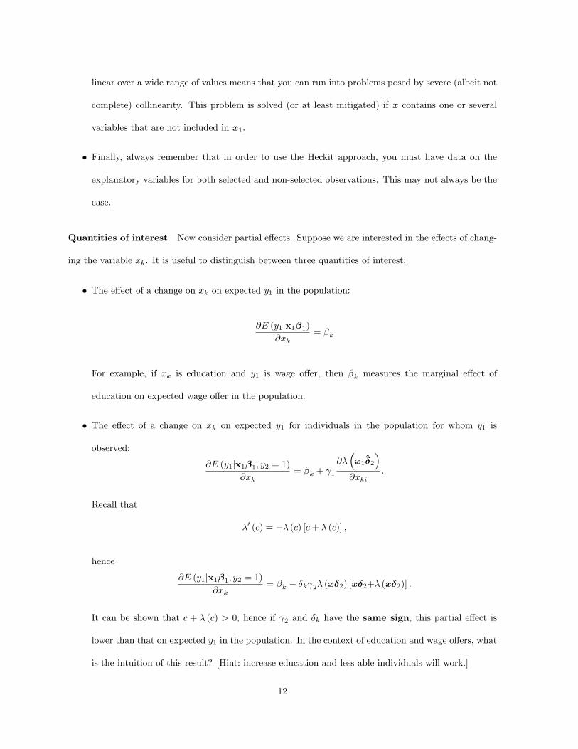
Quantities of interest Now consider partial e¤ects. Suppose we are interested in the e¤ects of chang-

ing the variable xk. It is useful to distinguish between three quantities of interest:

� The e¤ect of a change on xk on expected y1 in the population:

@E (y1jx1�1)@xk

= �k

For example, if xk is education and y1 is wage o¤er, then �k measures the marginal e¤ect of

education on expected wage o¤er in the population.

� The e¤ect of a change on xk on expected y1 for individuals in the population for whom y1 is

observed:

@E (y1jx1�1; y2 = 1)@xk

= �k + 1

@��x1�̂2

�@xki

:

Recall that

�0 (c) = �� (c) [c+ � (c)] ;

hence

@E (y1jx1�1; y2 = 1)@xk

= �k � �k 2� (x�2) [x�2+� (x�2)] :

It can be shown that c + � (c) > 0, hence if 2 and �k have the same sign, this partial e¤ect is

lower than that on expected y1 in the population. In the context of education and wage o¤ers, what

is the intuition of this result? [Hint: increase education and less able individuals will work.]

12

� For a slightly modi�ed version of the model, where y1 = 0, rather than unobserved, if y2 = 0,

we might be interested in the e¤ect of a change in xk on E (y1jx1�1) taking the zeros in y1 into

account. We have

E (y1jx1�1) = Pr (y2 = 1jx�2)� E (y1jx1�1; y2 = 1) + Pr (y2 = 0jx�2)� 0

E (y1jx1�1) = � (x�2)� E (y1jx1�1; y2 = 1) ;

and so "all" we need to do is �nd @E(y1jx1�1)@xk

. This involves some tedious algebra, and so I will not

go into detail. Check Cameron and Trivedi, Microeconometrics: Methods & Applications, p. 552 if

you are interested.

Estimation of Heckit in Stata In Stata we can use the command heckman to obtain Heckit esti-

mates. If the model is

yi = �0 + �1x1i + ui;

si =

8>><>>:1 if 0 + 1z1i + 2x1i + vi � 0

0 otherwise

9>>=>>; ;

the syntax has the following form

heckman y x1, select (z1 x1) twostep

where the variable y is missing whenever an observation is not included in the selected sample. If you

omit the twostep option you get full information maximum likelihood (FIML) estimates. Asymptotically,

these two methods are equivalent, but in small samples the results can di¤er. Simulations have taught us

that FIML is more e¢ cient than the two-stage approach but also more sensitive to mis-speci�cation due

to, say, non-normal disturbance terms. In applied work it makes sense to consider both sets of results.

EXAMPLES: See Section 2.1-2.3 in appendix.

13

2.3. Extensions of the Heckit model

2.3.1. Endogenous explanatory variables

Now consider the case where x1 contains a variable y2 that is correlated with the error term ui. That is,

y2 is endogenous in the population. We write the population model as

y1 = z1�1 + �1y2 + u1

y2 = z�2 + v2

y3 = 1 [z�3 + v3 � 0] :

The �rst equation here is the structural equation of interest; the second equation is the reduced form

equation for the endogenous explanatory variable y2; and the third equation is the selectivity equation.

� Assumption 17.2: (a) (z;y3) always observed, (y1; y2) observed when y3 = 1 (sample selection);

(b) (u1; v3) is independent of z (z exogenous); (c) v3 �Normal(0; 1) (distributional assumption);

E (u1jv3) = 1v3 (residuals may be correlated; e.g. bivariate normality); (e) E (z0v2 = 0), where

z�2 = z1�21 + z2�22; �22 6= 0 (valid and relevant instruments; exclusion restrictions)

Part (e) is new - instruments need to be orthogonal to the error term in the reduced form equation.

Note that the vector z2 must contain at least two variables (at least one instrument for y2; and at least

one variable determining selection). Under these assumptions, estimation of the model parameters is

relatively straightforward. We have

y1 = z1�1 + �1y2 + u1

y1 = z1�1 + �1y2 + E [u1jz;y3] + e1

in the population. Think of the term E [u1jz;y3] as the �sample selection�term.

14

In the selected sample,

E [u1jz;y3 = 1] = E [v3jz�3 + v3 � 0]

E [u1jz;y3 = 1] = 1E [v3jv3 � �z�3]

E [u1jz;y3 = 1] = 1� (z�3) ;

and so

y1 = z1�1 + �1y2 + 1� (z�3) + e1

for the selected sample. This leads naturally to the following estimation recipe:

1. Obtain �̂3 by estimating the participation equation using a probit model. Construct �̂i3 = ��z�̂3

�:

2. Using the selected sub-sample, estimate

y1 = z1�1 + �1y2 + 1�̂i3 + e1

using 2SLS, with instruments�z;�̂i3

�.

Note that if we only have one exclusion restriction, predicted y2 will be (nearly) collinear with z1 and

�̂i3. This is why we need at least two exclusion restrictions in the model.

EXAMPLE: See Section 2.4 in appendix.

2.3.2. Non-continuous outcome variables

We have focused on the case where y1, i.e. the outcome variable in the structural equation, is a continuous

variable. However, sample selection models can be formulated for many di¤erent models - binary response

models, censored models, duration models etc. The basic mechanism generating selection bias remains

the same: correlation between the unobservables determining selection and the unobservables determining

the outcome variable of interest.

15

Consider the following binary response model with sample selection:

y1 = 1 [x1�1 + u1 > 0]

y2 = 1 [x�2 + v2 > 0] ;

where y1 is observed only if y2 = 1, and x contains x1 and at least one more variable. In this case, probit

estimation of �1 based on the selected sample will generally lead to inconsistent results, unless u1 and

v2 are uncorrelated. Assuming that x is exogenous in the population (uncorrelated with u1 and v2), we

can use a two-stage procedure very similar to that discussed above:

1. Obtain �̂2 by estimating the participation equation using a probit model. Construct �̂i2 = ��z�̂2

�:

2. Estimate the structural equation using probit, with �̂i2 added to the set of regressors:

Pr (y1jx1;y2 = 1) = ��x1�1 + �1�̂i2

�;

where �1 measures the correlation between the residuals u1 and v2 (note: correlation will be the

same as the covariance, due to unity variance for the two residuals)

This is a good procedure for testing the null hypothesis that there is no selection bias (in which case

�1 = 0). If, based on this test we decide there is endogenous selection, we might choose to estimate

the two equations of the model simultaneously (in Stata: heckprob). This produces the right standard

errors, and recovers the structural parameters �1 rather than a scaled version of this vector.

2.3.3. Non-binary selection equation

Alternatively, it could be that the selection equation is not a binary response model - see Section IV in

Vella (1999) for an overview if you are interested. In computer exercise 5 we will study the case where

selection is modelled by means of a multinomial logit. An excellent survey paper in this context is

that by Bourguignon, Fournier and Gurgand. Please have a look at this paper before the computer lab

16

on Friday.

3. Estimation of Nonlinear Models with Panel Data

I will now discuss how probit, logit, tobit and heckit can be estimated when panel data are available. I

will focus on non-dynamic models and mostly on the binary choice models.1

3.1. Binary choice models for panel data

Using a latent variable framework, we write the panel binary choice model as

y�it = xit� + ci + uit;

yit = 1 [y�it > 0] ; (3.1)

and

Pr (yit = 1jxit; ci) = G (xit� + ci) ;

where G (:) is either the standard normal CDF (probit) or the logistic CDF (logit).

� Recall that, in linear models, it is easy to eliminate ci by means of �rst di¤erencing or using within

transformation.

� Those routes are not open to us here, unfortunately, since the model is nonlinear (e.g. di¤erencing

equation (3.1) does not remove ci).

� Moreover, if we attempt to estimate ci directly by adding N � 1 individual dummy variables to

the probit or logit speci�cation, this will result in severely biased estimates of � unless T is large.

This is known as the incidental parameters problem: with T small, the estimates of the ci

1As you know, including a lagged dependent variable in the set of explanatory variables complicates the estimation ofstandard linear panel data models. Conceptually similar problems arise for nonlinear models. Consider a dynamic probitmodel for example:

Pr (yit = 1jxit; ci) = � (�yi;t�1 + zit� + ci) ;The methods discussed below are generally not well suited for estimating such a model. If you are interested, check outhttp://www.soderbom.net/binarychoice2.pdf for a discussion.

17

are inconsistent (i.e. increasing N does not remove the bias), and, unlike the linear model, the

inconsistency in ci has a �knock-on e¤ect�in the sense that the estimate of � becomes inconsistent

too!

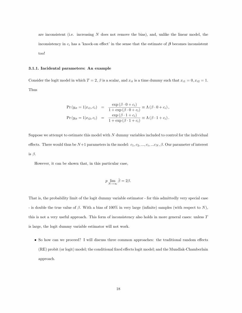
3.1.1. Incidental parameters: An example

Consider the logit model in which T = 2, � is a scalar, and xit is a time dummy such that xi1 = 0; xi2 = 1.

Thus

Pr (yit = 1jxi1; ci) =exp (� � 0 + ci)

1 + exp (� � 0 + ci)� � (� � 0 + ci) ;

Pr (yit = 1jxi2; ci) =exp (� � 1 + ci)

1 + exp (� � 1 + ci)� � (� � 1 + ci) :

Suppose we attempt to estimate this model with N dummy variables included to control for the individual

e¤ects. There would thus beN+1 parameters in the model: c1; c2; :::; ci; :::cN ; �:Our parameter of interest

is �.

However, it can be shown that, in this particular case,

p limN!1

�̂ = 2�:

That is, the probability limit of the logit dummy variable estimator - for this admittedly very special case

- is double the true value of �. With a bias of 100% in very large (in�nite) samples (with respect to N),

this is not a very useful approach. This form of inconsistency also holds in more general cases: unless T

is large, the logit dummy variable estimator will not work.

� So how can we proceed? I will discuss three common approaches: the traditional random e¤ects

(RE) probit (or logit) model; the conditional �xed e¤ects logit model; and the Mundlak-Chamberlain

approach.

18

3.1.2. The traditional random e¤ects (RE) probit

Model:

y�it = xit� + ci + uit;

yit = 1 [y�it > 0] ;

and

Pr (yit = 1jxit; ci) = G (xit� + ci) ;

Assumptions:

� ci and xit are independent

� the xit are strictly exogenous (this will be necessary for it to be possible to write the likelihood of

observing a given series of outcomes as the product of individual likelihoods).

� ci has a normal distribution with zero mean and variance �2c (note: homoskedasticity).

� yi1; :::; yiT are independent conditional on (xi; ci) - this rules out serial correlation in yit, conditional

on (xi; ci). This assumption enables us to write the likelihood of observing a given series of outcomes

as the product of individual likelihoods. The assumption can easily be relaxed - see eq. (15.68) in

Wooldridge (2002).

� Clearly these are restrictive assumptions, especially since endogeneity in the explanatory variables

is ruled out. The only advantage (which may strike you as rather marginal) over a simple pooled

probit model is that the RE model allows for serial correlation in the unobserved factors determining

yit, i.e. in (ci + uit).

� However, it is fairly straightforward to extend the model and allow for correlation between ci and

xit - this is precisely what the Mundlak-Chamberlain approach achieves, as we shall see below.

19

� Clearly, if ci had been observed, the likelihood of observing individual i would have been

TYt=1

[� (xit� + ci)]yit [1� � (xit� + ci)](1�yit) ;

and it would have been straightforward to maximize the sample likelihood conditional on xit; ci; yit.

� Because the ci are unobserved, however, they cannot be conditioned on in the likelihood function.

As discussed above, a dummy variables approach cannot be used, unless T is large. What can we

do?

� Recall from basic statistics (Bayes�theorem for probability densities) that, in general,

fxjy (x; y) =fxy (x; y)

fy (y);

where fxjy (x; y) is the conditional density of X given Y = y; fxy (x; y) is the joint distribution of

random variables X;Y ; and fy (y) is the marginal density of Y . Thus,

fxy (x; y) = fxjy (x; y) fy (y) :

� Moreover, the marginal density of X can be obtained by integrating out y from the joint density

fx (x) =

Zfxy (x; y) dy =

Zfxjy (x; y) fy (y) dy:

� Clearly we can think about fx (x) as a likelihood contribution. For a linear model, for example, we

might write

f" (") =

Zf"c ("; c) dc =

Zf"jc ("; c) fc (c) dc;

where "it = yit � (xit� + ci).

20

� In the context of the traditional RE probit, we integrate out ci from the likelihood as follows:

Li�yi1; :::; yiT jxi1; :::;xiT ;�;�2c

�=

Z TYt=1

[� (xit� + c)]yit [1� � (xit� + c)](1�yit) (1=�c)� (c=�c) dc:

� In general, there is no analytical solution here, and so numerical methods have to be used. The

most common approach is to use a Gauss-Hermite quadrature method, which amounts to

approximating

Z TYt=1

[� (xit� + c)]yit [1� � (xit� + c)](1�yit) (1=�c)� (c=�c) dc

as

��1=2MXm=1

wm

TYt=1

h��xit� +

p2�cgm

�iyit h1� �

�xit� +

p2�cgm

�i(1�yit); (3.2)

where M is the number of nodes, wm is a prespeci�ed weight, and gm a prespeci�ed node (prespec-

i�ed in such a way as to provide as good an approximation as possible of the normal distribution).

� For example, if M = 3, we have

wm gm

0.2954 -1.2247

1.1826 0.0000

0.2954 1.2247

21

in which case (3.2) can be written out as

0:1667TYt=1

[� (xit� � 1:731�c)]yit [1� � (xit� � 1:731�c)](1�yit)

+0:6667TYt=1

[� (xit�)]yit [1� � (xit�)](1�yit)

+0:1667TYt=1

[� (xit� + 1:731�c)]yit [1� � (xit� + 1:731�c)](1�yit) :

In practice a larger number of nodes than 3 would of course be used (the default in Stata isM = 12).

Lists of weights and nodes for given values of M can be found in the literature.

� To form the sample log likelihood, we simply compute weighted sums in this fashion for each indi-

vidual in the sample, and then add up all the individual likelihoods expressed in natural logarithms:

logL =NXi=1

logLi�yi1; :::; yiT jxi1; :::;xiT ;�;�2c

�:

Marginal e¤ects at ci = 0 can be computed using standard techniques. This model can be estimated

in Stata using the xtprobit command.

� EXAMPLE: Modelling exports in Ghana using probit and allowing for unobserved individual e¤ects.

Appendix Section 3.1

Whilst perhaps elegant, the above model does not allow for a correlation between ci and the explana-

tory variables, and so does not achieve anything in terms of addressing an endogeneity problem. We now

turn to more useful models in that context.

3.1.3. The "�xed e¤ects" logit model

Now return to the panel logit model:

Pr (yit = 1jxit; ci) = � (xit� + ci) :

22

� One important advantage of this model over the probit model is that will be possible to obtain a

consistent estimator of � without making any assumptions about how ci is related to xit (however,

you need strict exogeneity to hold; cf. within estimator for linear models).

� This is possible, because the logit functional form enables us to eliminate ci from the estimating

equation, once we condition on what is sometimes referred to as a "minimum su¢ cient statistic"

for ci.

To see this, assume T = 2, and consider the following conditional probabilities:

Pr (yi1 = 0; yi2 = 1jxi1; xi2; ci; yi1 + yi2 = 1) ;

and

Pr (yi1 = 1; yi2 = 0jxi1; xi2; ci; yi1 + yi2 = 1) :

The key thing to note here is that we condition on yi1 + yi2 = 1, i.e. that yit changes between the two

time periods. For the logit functional form, we have

Pr (yi1 + yi2 = 1jxi1; xi2; ci) =exp (xi1� + ci)

1 + exp (xi1� + ci)

1

1 + exp (xi2� + ci)

+1

1 + exp (xi1� + ci)

exp (xi2� + ci)

1 + exp (xi2� + ci);

or simply

Pr (yi1 + yi2 = 1jxi1; xi2; ci) =exp (xi1� + ci) + exp (xi2� + ci)

[1 + exp (xi1� + ci)] [1 + exp (xi2� + ci)]:

Furthermore,

Pr (yi1 = 0; yi2 = 1jxi1; xi2; ci) =1

1 + exp (xi1� + ci)

exp (xi2� + ci)

1 + exp (xi2� + ci);

23

hence, conditional on yi1 + yi2 = 1,

Pr (yi1 = 0; yi2 = 1jxi1; xi2; ci; yi1 + yi2 = 1)

=exp (xi2� + ci)

exp (xi1� + ci) + exp (xi2� + ci);

or

Pr (yi1 = 0; yi2 = 1jxi1; xi2; yi1 + yi2 = 1) =exp (�xi2�)

1 + exp (�xi2�)

� The key result here is that the ci are eliminated. It follows that

Pr (yi1 = 1; yi2 = 0jxi1; xi2; yi1 + yi2 = 1) =1

1 + exp (�xi2�):

� Remember:

1. These probabilities condition on yi1 + yi2 = 1

2. These probabilities are independent of ci.

Hence, by maximizing the following conditional log likelihood function

logL =

NXi=1

�d01i ln

�exp (�xi2�)

1 + exp (�xi2�)

�+ d10i ln

�1

1 + exp (�xi2�)

��;

we obtain consistent estimates of �, regardless of whether ci and xit are correlated.

� The trick is thus to condition the likelihood on the outcome series (yi1; yi2) ; and in the more

general case (yi1; yi2; :::; yiT ). For example, if T = 3, we can condition onP

t yit = 1, with possible

sequences f1; 0; 0g ; f0; 1; 0g and f0; 0; 1g, or onP

t yit = 2, with possible sequences f1; 1; 0g ; f1; 0; 1g

and f0; 1; 1g. Stata does this for us, of course. This estimator is requested in Stata by using xtlogit

with the fe option.

EXAMPLE: Exports in Ghana using FE logit. Appendix Section 3.2

24

Note that the logit functional form is crucial for it to be possible to eliminate the ci in this fashion.

It won�t be possible with probit. So this approach is not really very general. Another awkward issue

concerns the interpretation of the results. The estimation procedure just outlined implies we do not

obtain estimates of ci, which means we can�t compute marginal e¤ects.

3.1.4. Modelling the random e¤ect as a function of x-variables

The previous two methods are useful, but arguably they don�t quite help you achieve enough:

� the traditional random e¤ects probit/logit model requires strict exogeneity and zero correlation

between the explanatory variables and ci;

� the �xed e¤ects logit relaxes the latter assumption but we can�t obtain consistent estimates of ci

and hence we can�t compute the conventional marginal e¤ects in general.

We will now discuss an approach which, in some ways, can be thought of as representing a middle

way. Start from the latent variable model

y�it = xit� + ci + eit;

yit = 1[y�it>0]:

Consider writing the ci as an explicit function of the x-variables, for example as follows:

ci = + �xi� + ai; (3.3)

or

ci = �+ xi� + bi (3.4)

where �xi is an average of xit over time for individual i (hence time invariant); xi contains xit for all

t; ai is assumed uncorrelated with �xi; bi is assumed uncorrelated with xi. Equation (3.3) is easier to

25

implement and so we will focus on this (see Wooldridge, 2002, pp. 489-90 for a discussion of the more

general speci�cation).

� Assume that var (ai) = �2a is constant (i.e. there is homoskedasticity) and that ei is normally

distributed - the model that then results is known as Chamberlain�s random e¤ects probit

model. You might say (3.3) is restrictive, in the sense that functional form assumptions are made,

but at least it allows for non-zero correlation between ci and the regressors xit.

� The probability that yit = 1 can now be written as

Pr (yit = 1jxit; ci) = Pr (yit = 1jxit; �xi; ai) = � (xit� + + �xi� + ai) :

You now see that, after having added �xi to the RHS, we arrive at the traditional random e¤ects

probit model:

Li�yi1; :::; yiT jxi1; :::;xiT ;�;�2a

�=

Z TYt=1

[� (xit� + + �xi� + a)]yit

� [1� � (xit� + + �xi� + a)](1�yit) (1=�a)� (a=�a) da:

� E¤ectively, we are adding �xi as control variables to allow for some correlation between the random

e¤ect ci and the regressors.

� If xit contains time invariant variables, then clearly they will be collinear with their mean values

for individual i, thus preventing separate identi�cation of �-coe¢ cients on time invariant variables.

� We can easily compute marginal e¤ects at the mean of ci, since

E (ci) = + E (�xi) �

� Notice also that this model nests the simpler and more restrictive traditional random e¤ects probit:

26

under the (easily testable) null hypothesis that � = 0, the model reduces to the traditional model

discussed earlier.

� EXAMPLE: Exports in Ghana using probit and allowing for unobserved individual e¤ects correlated

with mean values of x-variables. Appendix Section 3.3

3.1.5. Relaxing the normality assumption for the unobserved e¤ect (optional)

The assumption that ci (or ai) is normally distributed is potentially strong. One alternative is to follow

Heckman and Singer (1984) and adopt a non-parametric strategy for characterizing the distribution of

the random e¤ects. The premise of this approach is that the distribution of c can be approximated by a

discrete multinomial distribution with Q points of support:

Pr (c = Cq) = Pq;

0 � Pq � 1,P

q Pq = 1, q = 1; 2; :::; Q, where the Cq, and the Pq are parameters to be estimated.

Hence, the estimated "support points" (the Cq) determine possible realizations for the random in-

tercept, and the Pq measure the associated probabilities. The likelihood contribution of individual i is

now

Li�yi1; :::; yiT jxi1; :::;xiT ;�;�2c

�=

QXq

Pq

TYt=1

[� (xit� + Cq)]yit [1� � (xit� + Cq)](1�yit) :

Compared to the model based on the normal distribution for ci, this model is clearly quite �exible.

In estimating the model, one important issue refers to the number of support points, Q. In fact,

there are no well-established theoretically based criteria for determining the number of support points in

models like this one. Standard practice is to increase Q until there are only marginal improvements in

the log likelihood value. Usually, the number of support points is small - certainly below 10 and typically

below 5.

27

Notice that there are many parameters in this model. With 4 points of support, for example, you

estimate 3 probabilities (the 4th is a �residual�probability resulting from the constraint that probabilities

sum to 1) and 3 support points (one is omitted if - as typically is the case - xit contains a constant). So

that�s 6 parameters compared to 1 parameter for the traditional random e¤ects probit based on normality.

That is the consequence of attempting to estimate the entire distribution of c.

Unfortunately, implementing this model is often di¢ cult:

� Sometimes the estimator will not converge.

� Convergence may well occur at a local maximum.

� Inverting the Hessian in order to get standard errors may not always be possible.

So clearly the additional �exibility comes at a cost.

Allegedly, the Stata program gllamm can be used to produce results for this type of estimator.2

3.2. Extension: Panel Tobit Models

The treatment of tobit models for panel data is very similar to that for probit models. We state the

(non-dynamic) unobserved e¤ects model as

yit = max (0;xit� + ci + uit) ;

uitjxit; ci � Normal�0; �2u

�:

We cannot control for ci by means of a dummy variable approach (incidental parameters problem),

and no tobit model analogous to the "�xed e¤ects" logit exists. We therefore consider the random e¤ects

tobit estimator (Note: Bo Honoré has proposed a "�xed e¤ects" tobit that does not impose distributional

assumptions. Unfortunately it is hard to implement. Moreover, partial e¤ects cannot be estimated. I

therefore do not cover this approach. See Honoré�s web page if you are interested).

2http://www.gllamm.org/

28

3.2.1. Traditional RE tobit

For the traditional random e¤ects tobit model, the underlying assumptions are the same as those under-

lying the traditional RE probit. That is,

� ci and xit are independent

� the xit are strictly exogenous (this will be necessary for it to be possible to write the likelihood of

observing a given series of outcomes as the product of individual likelihoods).

� ci has a normal distribution with zero mean and variance �2c

� yi1; :::; yiT are independent conditional on (xi; ci) ; ruling out serial correlation in yit, conditional

on (xi; ci) : This assumption can be relaxed:

Under these assumptions, we can proceed in exactly the same way as for the traditional RE probit, once

we have changed the log likelihood function from probit to tobit. Hence, the contribution of individual i

to the sample likelihood is

Li�yi1; :::; yiT jxi1; :::;xiT ;�;�2c

�=

Z TYt=1

�1� �

�xit� + c

�u

��1[yi=0][� ((yit � xit� � c) =�u) =�u]

1[yi=1] (1=�c)� (c=�c) dc:

This model can be estimated using the xttobit command in Stata.

3.2.2. Modelling the random e¤ect as a function of x-variables

The assumption that ci and xit are independent is unattractive. Just like for the probit model, we can

adopt a Mundlak-Chamberlain approach and specify ci as a function of observables, eg.

ci = + �xi� + ai:

29

This means we rewrite the panel tobit as

yit = max (0;xit� + + �xi� + ai + uit) ;

uitjxit; ai � Normal�0; �2u

�:

From this point, everything is analogous to the probit model (except of course the form of the likelihood

function, which will be tobit and not probit) and so there is no need to go over the estimation details

again. Bottom line is that we can use the xttobit command and just add individual means of time

varying x-variables to the set of regressors. Partial e¤ects of interest evaluated at the mean of ci are easy

to compute, since

E (ci) = + E (�xi) �:

3.3. Extension: Heckit with panel data

Model:

yit = xit� + ci + uit; (Primary equation)

where selection is determined by the equation

sit =

8>><>>:1 if zit + di + vit � 0

0 otherwise

9>>=>>; : (Selection equation)

Assumptions regarding unobserved e¤ects and residuals are as for the RE tobit-

� If selection bias arises because ci is correlated with di, then estimating the main equation using a

�xed e¤ects or �rst di¤erenced approach on the selected sample will produce consistent estimates

of �.

� However, if corr (uit; vit) 6= 0, we can address the sample selection problem using a panel Heckit

approach. Again, the Mundlak-Chamberlain approach is convenient - that is,

30

�Write down speci�cations for ci and di and plug these into the equations above

�Estimate T di¤erent selection probits (i.e. do not use xtprobit here, use pooled probit).

Compute T inverse Mills ratios.

�Estimate

yit = xit� + xi�+D1�1�̂1 + :::+DT �T �̂T + eit;

on the selected sample. This yields consistent estimates of �, provided the model is correctly

speci�ed.

31

1

PhD Programme: Applied Econometrics Department of Economics, University of Gothenburg Appendix: Lecture 15 Måns Söderbom 1. Derivation of the Inverse Mills Ratio (IMR)

To show )()(

)(1)()|(

cc

ccczzE

−Φ−

=Φ−

=>φφ

Assume that z is normally distributed:

( ) ( ) ( )z

G z z z dzφ−∞

= Φ ≡ ∫

21( ) exp( )22zzφ

π= −

( )G z is the normal cumulative density function (CDF), ( )zφ is the standard normal density

function. We now wish to know the ( | )E z z c> . It is the shaded area in the graph below.

c z By the characteristics of the normal curve is equal to[1 ( )]c−Φ . So the density of z is given by

czc

z>

Φ− ,

)](1[)(φ

so

2

dzc

zzczzEc∫∞

Φ−=>

)](1[)()|( φ

which can be written using the definitions above as:

21( | ) .exp( )(1 ( )) 22c

z zE z z c dzc π

∞ −> =

−Φ ∫

This expression can be written as:

1 ( )( | ) ( )(1 ( ))

c

d zE z z c dzc dz

φ∞

> = −−Φ ∫

How do we know that:

2( ) 1 exp( )

22d z z z

dzφ

π= − ⋅−

2 2( ) 1 1( ) exp( ) 0 exp( ) ( )2 22 2c c

d z z cdz cdzφ φ

π π

∞ ∞

− = − − = + − =∫ ∫

So:

Lets evaluate2

.exp( )22c

z z dzπ

∞ −∫ =

This can be written as

)](1[)()(

)](1[1

cczd

c c Φ−=Φ

Φ−− ∫

∞ φ

Recall that for the normal distribution )()( cc −= φφ and )()(1 cc −Φ=Φ− From which it follows that

)()(

)](1[)()|(

ccdz

czzczzE

c −Φ−

=Φ−

=> ∫∞ φφ

It is this last expression which is the inverse Mills ratio.

3

Figure 1: The Inverse Mills Ratio

01

23

4im

r

-4 -2 0 2 4z

4

-10

12

3ln

wag

e

6 8 10 12 14education

Included in selected sample Not included in selected sampleRelationship in population Relationship in selected sample

m>0

m>0

m<0

m<0

This observation is not included in the selected sample

Figure 2: Illustration of Sample Selection Bias

The economic model underlying the graph isln w = cons + 0.1educ + m,

where w is wage, educ is education and m is unobserved motivation. Selection into the sample is a positive function of educ and m.

5

2. Two empirical illustrations of the Heckit model

2.1 Earnings regressions for wage-employed men aged 16-30 in Pakistan Data: The Pakistan Integrated Household Survey 1998/99. For an analysis of these data, see Kingdon, Geeta and Måns Söderbom, “Education, Skills, and Labor Market Outcomes: Evidence from Pakistan,” Education Working Paper Series, no. 11, May 2008. Washington D.C: The World Bank. This can be downloaded at http://www.soderbom.net/ADElab1.pdf. Summary statistics Variable | Obs Mean Std. Dev. Min Max -------------+-------------------------------------------------------- lw | 4853 10.1027 .7019855 4.787492 12.8739 educ | 10018 5.891296 4.722177 0 19 age | 10018 22.84019 4.340287 16 30 married | 10018 .3760232 .4844101 0 1 kidsund12 | 10018 2.571571 2.63225 0 20 -------------+-------------------------------------------------------- eldove65 | 10018 .1998403 .4615515 0 3

i) OLS . reg lw educ age married if sex==1 & age<=30 Source | SS df MS Number of obs = 4853 -------------+------------------------------ F( 3, 4849) = 501.00 Model | 565.752465 3 188.584155 Prob > F = 0.0000 Residual | 1825.23373 4849 .376414463 R-squared = 0.2366 -------------+------------------------------ Adj R-squared = 0.2361 Total | 2390.9862 4852 .492783635 Root MSE = .61353 ------------------------------------------------------------------------------ lw | Coef. Std. Err. t P>|t| [95% Conf. Interval] -------------+---------------------------------------------------------------- educ | .0370919 .0018438 20.12 0.000 .0334772 .0407066 age | .0508328 .0025309 20.09 0.000 .0458711 .0557944 married | .1569765 .0216604 7.25 0.000 .1145123 .1994407 _cons | 8.614617 .0544189 158.30 0.000 8.507931 8.721303 ------------------------------------------------------------------------------

6

ii) Heckit . heckman lw educ age married if sex==1 & age<=30, select(age educ kidsund12 eldove65 married) twostep Heckman selection model -- two-step estimates Number of obs = 10018 (regression model with sample selection) Censored obs = 5165 Uncensored obs = 4853 Wald chi2(6) = 888.37 Prob > chi2 = 0.0000 ------------------------------------------------------------------------------ | Coef. Std. Err. z P>|z| [95% Conf. Interval] -------------+---------------------------------------------------------------- lw | educ | .036956 .0018689 19.77 0.000 .0332929 .040619 age | .0494845 .0038901 12.72 0.000 .0418601 .0571088 married | .154299 .0224542 6.87 0.000 .1102895 .1983084 _cons | 8.68906 .1718886 50.55 0.000 8.352165 9.025956 -------------+---------------------------------------------------------------- select | age | .0406764 .0035879 11.34 0.000 .0336443 .0477085 educ | .003192 .0027291 1.17 0.242 -.0021569 .008541 kidsund12 | -.0487458 .0050142 -9.72 0.000 -.0585734 -.0389181 eldove65 | -.0580974 .0276959 -2.10 0.036 -.1123805 -.0038144 married | .1366124 .0325453 4.20 0.000 .0728248 .2003999 _cons | -.9026498 .0775054 -11.65 0.000 -1.054558 -.7507419 -------------+---------------------------------------------------------------- mills | lambda | -.0509581 .1115998 -0.46 0.648 -.2696897 .1677734 -------------+---------------------------------------------------------------- rho | -0.08291 sigma | .61459573 lambda | -.05095814 .1115998 ------------------------------------------------------------------------------

7

2.2 Earnings regressions for females in the US This section uses the MROZ dataset.1 This dataset contains information on 753 women. We observe the wage offer for only 428 women, hence the sample is truncated. use C:\teaching_gbg07\applied_econ07\MROZ.dta

1 See examples 17.6 and 17.7 in Wooldridge (2002). Original source of data: Mroz, T.A. (1987) "The sensitivity of an empirical model of married women's hours of work to economic and statistical assumptions," Econometrica 55, 765-799.

1. OLS on selected sample reg lwage educ exper expersq Source | SS df MS Number of obs = 428 -------------+------------------------------ F( 3, 424) = 26.29 Model | 35.0223023 3 11.6741008 Prob > F = 0.0000 Residual | 188.305149 424 .444115917 R-squared = 0.1568 -------------+------------------------------ Adj R-squared = 0.1509 Total | 223.327451 427 .523015108 Root MSE = .66642 ------------------------------------------------------------------------------ lwage | Coef. Std. Err. t P>|t| [95% Conf. Interval] -------------+---------------------------------------------------------------- educ | .1074896 .0141465 7.60 0.000 .0796837 .1352956 exper | .0415665 .0131752 3.15 0.002 .0156697 .0674633 expersq | -.0008112 .0003932 -2.06 0.040 -.0015841 -.0000382 _cons | -.5220407 .1986321 -2.63 0.009 -.9124668 -.1316145 ------------------------------------------------------------------------------

8

2. Two-step Heckit . heckman lwage educ exper expersq, select(nwifeinc educ exper expersq age kidslt6 kidsge6) twostep Heckman selection model -- two-step estimates Number of obs = 753 (regression model with sample selection) Censored obs = 325 Uncensored obs = 428 Wald chi2(6) = 180.10 Prob > chi2 = 0.0000 ------------------------------------------------------------------------------ | Coef. Std. Err. z P>|z| [95% Conf. Interval] -------------+---------------------------------------------------------------- lwage | educ | .1090655 .015523 7.03 0.000 .0786411 .13949 exper | .0438873 .0162611 2.70 0.007 .0120163 .0757584 expersq | -.0008591 .0004389 -1.96 0.050 -.0017194 1.15e-06 _cons | -.5781033 .3050062 -1.90 0.058 -1.175904 .0196979 -------------+---------------------------------------------------------------- select | nwifeinc | -.0120237 .0048398 -2.48 0.013 -.0215096 -.0025378 educ | .1309047 .0252542 5.18 0.000 .0814074 .180402 exper | .1233476 .0187164 6.59 0.000 .0866641 .1600311 expersq | -.0018871 .0006 -3.15 0.002 -.003063 -.0007111 age | -.0528527 .0084772 -6.23 0.000 -.0694678 -.0362376 kidslt6 | -.8683285 .1185223 -7.33 0.000 -1.100628 -.636029 kidsge6 | .036005 .0434768 0.83 0.408 -.049208 .1212179 _cons | .2700768 .508593 0.53 0.595 -.7267472 1.266901 -------------+---------------------------------------------------------------- mills | lambda | .0322619 .1336246 0.24 0.809 -.2296376 .2941613 -------------+---------------------------------------------------------------- rho | 0.04861 sigma | .66362876 lambda | .03226186 .1336246 ------------------------------------------------------------------------------

9

3. Simultaneous estimation of selection model . heckman lwage educ exper expersq, select(nwifeinc educ exper expersq age kidslt6 kidsge6) Iteration 0: log likelihood = -832.89777 Iteration 1: log likelihood = -832.8851 Iteration 2: log likelihood = -832.88509 Heckman selection model Number of obs = 753 (regression model with sample selection) Censored obs = 325 Uncensored obs = 428 Wald chi2(3) = 59.67 Log likelihood = -832.8851 Prob > chi2 = 0.0000 ------------------------------------------------------------------------------ | Coef. Std. Err. z P>|z| [95% Conf. Interval] -------------+---------------------------------------------------------------- lwage | educ | .1083502 .0148607 7.29 0.000 .0792238 .1374767 exper | .0428369 .0148785 2.88 0.004 .0136755 .0719983 expersq | -.0008374 .0004175 -2.01 0.045 -.0016556 -.0000192 _cons | -.5526974 .2603784 -2.12 0.034 -1.06303 -.0423652 -------------+---------------------------------------------------------------- select | nwifeinc | -.0121321 .0048767 -2.49 0.013 -.0216903 -.002574 educ | .1313415 .0253823 5.17 0.000 .0815931 .1810899 exper | .1232818 .0187242 6.58 0.000 .0865831 .1599806 expersq | -.0018863 .0006004 -3.14 0.002 -.003063 -.0007095 age | -.0528287 .0084792 -6.23 0.000 -.0694476 -.0362098 kidslt6 | -.8673988 .1186509 -7.31 0.000 -1.09995 -.6348472 kidsge6 | .0358723 .0434753 0.83 0.409 -.0493377 .1210824 _cons | .2664491 .5089578 0.52 0.601 -.7310898 1.263988 -------------+---------------------------------------------------------------- /athrho | .026614 .147182 0.18 0.857 -.2618573 .3150854 /lnsigma | -.4103809 .0342291 -11.99 0.000 -.4774687 -.3432931 -------------+---------------------------------------------------------------- rho | .0266078 .1470778 -.2560319 .3050564 sigma | .6633975 .0227075 .6203517 .7094303 lambda | .0176515 .0976057 -.1736521 .2089552 ------------------------------------------------------------------------------ LR test of indep. eqns. (rho = 0): chi2(1) = 0.03 Prob > chi2 = 0.8577 ------------------------------------------------------------------------------

10

4. Selection model with endogenous education . probit inlf nwifeinc exper expersq age kidslt6 kidsge6 motheduc fatheduc huseduc Iteration 0: log likelihood = -514.8732 Iteration 1: log likelihood = -414.44513 Iteration 2: log likelihood = -411.33354 Iteration 3: log likelihood = -411.32238 Iteration 4: log likelihood = -411.32238 Probit regression Number of obs = 753 LR chi2(9) = 207.10 Prob > chi2 = 0.0000 Log likelihood = -411.32238 Pseudo R2 = 0.2011 ------------------------------------------------------------------------------ inlf | Coef. Std. Err. z P>|z| [95% Conf. Interval] -------------+---------------------------------------------------------------- nwifeinc | -.0074294 .0048787 -1.52 0.128 -.0169915 .0021327 exper | .1285092 .0185226 6.94 0.000 .0922056 .1648129 expersq | -.0019474 .0005955 -3.27 0.001 -.0031146 -.0007803 age | -.0527657 .0085423 -6.18 0.000 -.0695082 -.0360231 kidslt6 | -.8149255 .1160833 -7.02 0.000 -1.042445 -.5874063 kidsge6 | .0241511 .0432253 0.56 0.576 -.060569 .1088712 motheduc | .0295321 .0185718 1.59 0.112 -.006868 .0659322 fatheduc | .0133487 .0178491 0.75 0.455 -.0216349 .0483324 huseduc | .0161391 .019595 0.82 0.410 -.0222664 .0545446 _cons | 1.146672 .4932706 2.32 0.020 .1798798 2.113465 ------------------------------------------------------------------------------ . . predict zg, xb . ge imr=normalden(zg)/normal(zg) . . ivreg2 lwage exper expersq imr (educ = nwifeinc exper expersq age kidslt6 kidsge6 motheduc fatheduc huseduc)

11

Warning - duplicate variables detected Duplicates: exper expersq IV (2SLS) estimation -------------------- Estimates efficient for homoskedasticity only Statistics consistent for homoskedasticity only Number of obs = 428 F( 4, 423) = 9.44 Prob > F = 0.0000 Total (centered) SS = 223.3274513 Centered R2 = 0.1531 Total (uncentered) SS = 829.594813 Uncentered R2 = 0.7720 Residual SS = 189.1272506 Root MSE = .6647 ------------------------------------------------------------------------------ lwage | Coef. Std. Err. z P>|z| [95% Conf. Interval] -------------+---------------------------------------------------------------- educ | .0877632 .0212981 4.12 0.000 .0460196 .1295067 exper | .0457425 .0164923 2.77 0.006 .0134182 .0780668 expersq | -.0009128 .0004441 -2.06 0.040 -.0017833 -.0000423 imr | .0404355 .1326462 0.30 0.760 -.2195463 .3004173 _cons | -.3249135 .3315012 -0.98 0.327 -.974644 .324817 ------------------------------------------------------------------------------ Underidentification test (Anderson canon. corr. LM statistic): 188.702 Chi-sq(7) P-val = 0.0000 ------------------------------------------------------------------------------ Weak identification test (Cragg-Donald Wald F statistic): 46.976 Stock-Yogo weak ID test critical values: 5% maximal IV relative bias 19.86 10% maximal IV relative bias 11.29 20% maximal IV relative bias 6.73 30% maximal IV relative bias 5.07 10% maximal IV size 31.50 15% maximal IV size 17.38 20% maximal IV size 12.48 25% maximal IV size 9.93 Source: Stock-Yogo (2005). Reproduced by permission. ------------------------------------------------------------------------------ Sargan statistic (overidentification test of all instruments): 6.961 Chi-sq(6) P-val = 0.3245 ------------------------------------------------------------------------------ Instrumented: educ Included instruments: exper expersq imr Excluded instruments: nwifeinc age kidslt6 kidsge6 motheduc fatheduc huseduc Duplicates: exper expersq ------------------------------------------------------------------------------

12

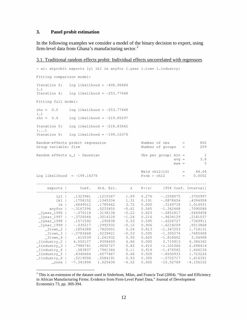
3. Panel probit estimation In the following examples we consider a model of the binary decision to export, using firm-level data from Ghana’s manufacturing sector.2

2 This is an extension of the dataset used in Söderbom, Måns, and Francis Teal (2004). “Size and Efficiency in African Manufacturing Firms: Evidence from Firm-Level Panel Data,” Journal of Development Economics 73, pp. 369-394.

3.1. Traditional random effects probit: Individual effects uncorrelated with regressors > xi: xtprobit exports lyl lkl le anyfor i.year i.town i.industry; Fitting comparison model: Iteration 0: log likelihood = -408.96484 (…) Iteration 4: log likelihood = -253.77448 Fitting full model: rho = 0.0 log likelihood = -253.77448 (…) rho = 0.6 log likelihood = -219.85297 Iteration 0: log likelihood = -218.83642 (...) Iteration 6: log likelihood = -199.16376 Random-effects probit regression Number of obs = 802 Group variable: firm Number of groups = 209 Random effects u_i ~ Gaussian Obs per group: min = 1 avg = 3.8 max = 5 Wald chi2(16) = 44.64 Log likelihood = -199.16376 Prob > chi2 = 0.0002 ------------------------------------------------------------------------------ exports | Coef. Std. Err. z P>|z| [95% Conf. Interval] -------------+---------------------------------------------------------------- lyl | .1323961 .1215347 1.09 0.276 -.1058075 .3705997 lkl | .1758152 .1345334 1.31 0.191 -.0878654 .4394958 le | .6649512 .1785642 3.72 0.000 .3149718 1.014931 anyfor | -.3167296 .5233455 -0.61 0.545 -1.342468 .7090088 _Iyear_1996 | -.070118 .3138138 -0.22 0.823 -.6851817 .5449458 _Iyear_1997 | -.3726546 .3014128 -1.24 0.216 -.9634129 .2181037 _Iyear_1998 | .1571592 .295838 0.53 0.595 -.4226727 .7369911 _Iyear_1999 | -.035217 .2992932 -0.12 0.906 -.6218209 .5513868 _Itown_2 | .1854388 .7820001 0.24 0.813 -1.347253 1.718131 _Itown_3 | -.2783668 .5239421 -0.53 0.595 -1.305274 .7485408 _Itown_4 | .615539 1.241932 0.50 0.620 -1.818602 3.04968 _Iindustry_2 | 4.550127 .9358409 4.86 0.000 2.715913 6.384342 _Iindustry_3 | .7986741 .9692727 0.82 0.410 -1.101066 2.698414 _Iindustry_4 | .083837 .7961364 0.11 0.916 -1.476562 1.644236 _Iindustry_5 | .4340664 .6577467 0.66 0.509 -.8550933 1.723226 _Iindustry_6 | .5219096 .5584191 0.93 0.350 -.5725717 1.616391 _cons | -7.341894 1.625434 -4.52 0.000 -10.52769 -4.156102

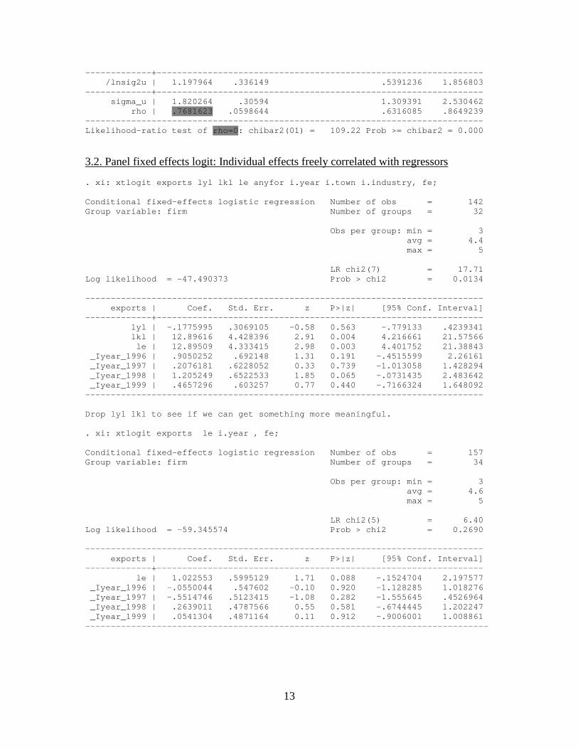
13

-------------+---------------------------------------------------------------- /lnsig2u | 1.197964 .336149 .5391236 1.856803 -------------+---------------------------------------------------------------- sigma_u | 1.820264 .30594 1.309391 2.530462 rho | .7681623 .0598644 .6316085 .8649239 ------------------------------------------------------------------------------ Likelihood-ratio test of rho=0: chibar2(01) = 109.22 Prob >= chibar2 = 0.000 3.2. Panel fixed effects logit: Individual effects freely correlated with regressors . xi: xtlogit exports lyl lkl le anyfor i.year i.town i.industry, fe; Conditional fixed-effects logistic regression Number of obs = 142 Group variable: firm Number of groups = 32 Obs per group: min = 3 avg = 4.4 max = 5 LR chi2(7) = 17.71 Log likelihood = -47.490373 Prob > chi2 = 0.0134 ------------------------------------------------------------------------------ exports | Coef. Std. Err. z P>|z| [95% Conf. Interval] -------------+---------------------------------------------------------------- lyl | -.1775995 .3069105 -0.58 0.563 -.779133 .4239341 lkl | 12.89616 4.428396 2.91 0.004 4.216661 21.57566 le | 12.89509 4.333415 2.98 0.003 4.401752 21.38843 _Iyear_1996 | .9050252 .692148 1.31 0.191 -.4515599 2.26161 _Iyear_1997 | .2076181 .6228052 0.33 0.739 -1.013058 1.428294 _Iyear_1998 | 1.205249 .6522533 1.85 0.065 -.0731435 2.483642 _Iyear_1999 | .4657296 .603257 0.77 0.440 -.7166324 1.648092 ------------------------------------------------------------------------------ Drop lyl lkl to see if we can get something more meaningful. . xi: xtlogit exports le i.year , fe; Conditional fixed-effects logistic regression Number of obs = 157 Group variable: firm Number of groups = 34 Obs per group: min = 3 avg = 4.6 max = 5 LR chi2(5) = 6.40 Log likelihood = -59.345574 Prob > chi2 = 0.2690 ------------------------------------------------------------------------------ exports | Coef. Std. Err. z P>|z| [95% Conf. Interval] -------------+---------------------------------------------------------------- le | 1.022553 .5995129 1.71 0.088 -.1524704 2.197577 _Iyear_1996 | -.0550044 .547602 -0.10 0.920 -1.128285 1.018276 _Iyear_1997 | -.5514746 .5123415 -1.08 0.282 -1.555645 .4526964 _Iyear_1998 | .2639011 .4787566 0.55 0.581 -.6744445 1.202247 _Iyear_1999 | .0541304 .4871164 0.11 0.912 -.9006001 1.008861 -------------------------------------------------------------------------------

14

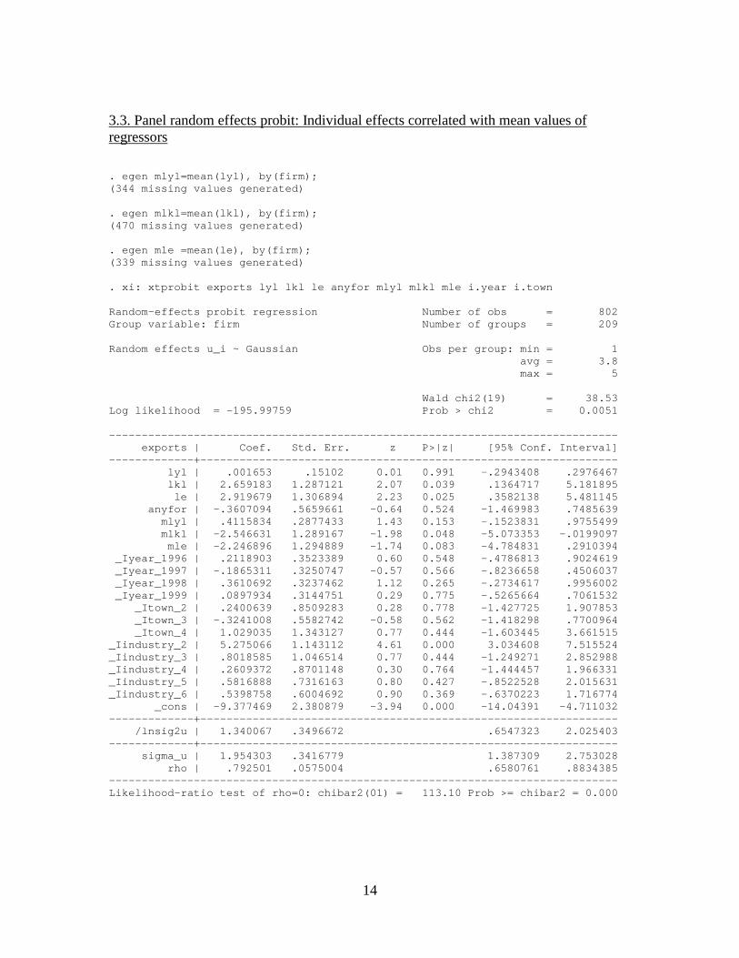
3.3. Panel random effects probit: Individual effects correlated with mean values of regressors . egen mlyl=mean(lyl), by(firm); (344 missing values generated) . egen mlkl=mean(lkl), by(firm); (470 missing values generated) . egen mle =mean(le), by(firm); (339 missing values generated) . xi: xtprobit exports lyl lkl le anyfor mlyl mlkl mle i.year i.town Random-effects probit regression Number of obs = 802 Group variable: firm Number of groups = 209 Random effects u_i ~ Gaussian Obs per group: min = 1 avg = 3.8 max = 5 Wald chi2(19) = 38.53 Log likelihood = -195.99759 Prob > chi2 = 0.0051 ------------------------------------------------------------------------------ exports | Coef. Std. Err. z P>|z| [95% Conf. Interval] -------------+---------------------------------------------------------------- lyl | .001653 .15102 0.01 0.991 -.2943408 .2976467 lkl | 2.659183 1.287121 2.07 0.039 .1364717 5.181895 le | 2.919679 1.306894 2.23 0.025 .3582138 5.481145 anyfor | -.3607094 .5659661 -0.64 0.524 -1.469983 .7485639 mlyl | .4115834 .2877433 1.43 0.153 -.1523831 .9755499 mlkl | -2.546631 1.289167 -1.98 0.048 -5.073353 -.0199097 mle | -2.246896 1.294889 -1.74 0.083 -4.784831 .2910394 _Iyear_1996 | .2118903 .3523389 0.60 0.548 -.4786813 .9024619 _Iyear_1997 | -.1865311 .3250747 -0.57 0.566 -.8236658 .4506037 _Iyear_1998 | .3610692 .3237462 1.12 0.265 -.2734617 .9956002 _Iyear_1999 | .0897934 .3144751 0.29 0.775 -.5265664 .7061532 _Itown_2 | .2400639 .8509283 0.28 0.778 -1.427725 1.907853 _Itown_3 | -.3241008 .5582742 -0.58 0.562 -1.418298 .7700964 _Itown_4 | 1.029035 1.343127 0.77 0.444 -1.603445 3.661515 _Iindustry_2 | 5.275066 1.143112 4.61 0.000 3.034608 7.515524 _Iindustry_3 | .8018585 1.046514 0.77 0.444 -1.249271 2.852988 _Iindustry_4 | .2609372 .8701148 0.30 0.764 -1.444457 1.966331 _Iindustry_5 | .5816888 .7316163 0.80 0.427 -.8522528 2.015631 _Iindustry_6 | .5398758 .6004692 0.90 0.369 -.6370223 1.716774 _cons | -9.377469 2.380879 -3.94 0.000 -14.04391 -4.711032 -------------+---------------------------------------------------------------- /lnsig2u | 1.340067 .3496672 .6547323 2.025403 -------------+---------------------------------------------------------------- sigma_u | 1.954303 .3416779 1.387309 2.753028 rho | .792501 .0575004 .6580761 .8834385 ------------------------------------------------------------------------------ Likelihood-ratio test of rho=0: chibar2(01) = 113.10 Prob >= chibar2 = 0.000