applications of statistics to medicine and medical physics

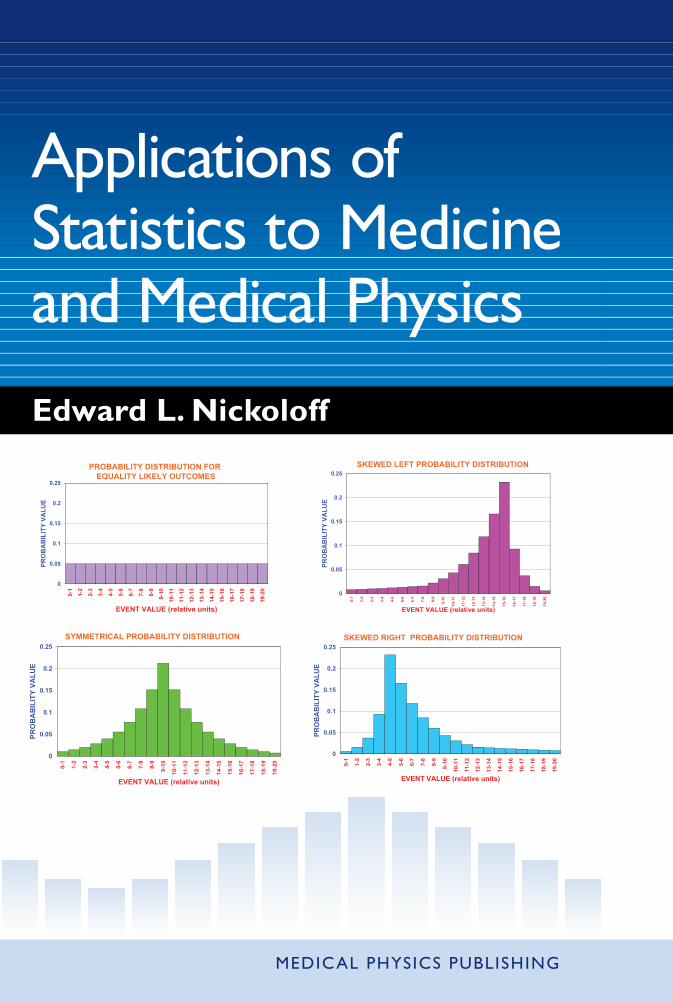
Edward L. Nickoloff

MEDICAL PHYSICS PUBLISHING

Applications of Statistics to Medicine and Medical Physics

Applications of Statistics to

Medicine and M

edical PhysicsN

ickolo

ff

Nickoloff_cover_case_final.indd 1 3/8/11 10:47 AM

Applications of Statistics

to Medicine and Medical Physics

Applications of Statisticsto Medicine and Medical Physics

Edward L. Nickoloff, D.Sc.FACR, FAAPM, and FACMP

Professor of RadiologyColumbia University and

New York-Presbyterian HospitalNew York, New York

MEDICAL PHYSICS PUBLISHINGMadison, Wisconsin

Copyright © 2011 by Edward L. Nickoloff

All rights reserved. No part of this publication may be reproduced or distributed in anyform or by any means without written permission from the publisher.

15 14 13 12 11 1 2 3 4 5 6

Library of Congress Control Number: 2011924799

ISBN 13: 978-1-930524-51-4 hardcoverISBN 13: 978-1-980524-71-2 2014 eBook edition

Medical Physics Publishing4513 Vernon BoulevardMadison, WI 53705-4964Phone: 1-800-442-5778, 608-262-4021Fax: 608-265-2121Email: [email protected]: www.medicalphysics.org

Notice: Information in this book is provided for instructional use only. The author and publisher have taken care that the information and recommendations containedherein are accurate and compatible with the standards generally accepted at the time of publication. Nevertheless, it is difficult to ensure that all the information given isentirely accurate for all circumstances. The author and publisher cannot assumeresponsibility for the validity of all materials or for any damage or harm incurred as a result of the use of this information.

Printed in the United States of America on acid-free paper

This book is dedicated to my son, Edward Jr., and my daughter, Andrea Lee.

They have both taught me many life lessons, such as perseverance of goals despite numerous obstacles and adversities in the path toward those goals. The future will depend upon the character,

motivation, capabilities, and efforts of our young people.I believe that the future will be marvelous because of the

exuberance and determination of the next generation.

Dedication

Preface............................................................................................................ xiii

1 Fundamental Concepts and Their Applications

1.1 Permutations................................................................................................... 11.2 Combinations.................................................................................................. 21.3 Frequency Distribution................................................................................... 41.4 Median, Mode, and Mean............................................................................... 61.5 Quartiles ......................................................................................................... 71.6 Cumulative Frequency Distribution ............................................................... 7

Useful References........................................................................................... 8Practice Exercises........................................................................................... 9

2 Probability Distribution

2.1 Introduction to Characteristics of Probability Distributions .......................... 132.2 Binomial Probability Distribution .................................................................. 18

2.2.1 Fundamentals........................................................................................ 182.2.2 Application A........................................................................................ 222.2.3 Application B........................................................................................ 232.2.4 Application C........................................................................................ 24

vii

Contents

viii ■ Contents

2.3 Poisson Probability Distribution .................................................................... 252.3.1 Fundamentals........................................................................................ 252.3.2 Applications.......................................................................................... 27

2.4 Normal Probability Distribution..................................................................... 292.4.1 Fundamentals........................................................................................ 292.4.2 Application A........................................................................................ 312.4.3 Application B........................................................................................ 32

2.5 Log Normal Probability Distribution ............................................................. 342.5.1 Fundamentals........................................................................................ 342.5.2 Application ........................................................................................... 37

2.6 Error Function ................................................................................................ 382.6.1 Basics.................................................................................................... 382.6.2 Application ........................................................................................... 43Useful References........................................................................................... 45Practice Exercises........................................................................................... 46

3 More Details about the Normal Probability Distribution

3.1 The Mean........................................................................................................ 493.2 The Standard Deviation.................................................................................. 503.3 Statistical Sampling........................................................................................ 513.4 Applications of Mean and Standard Deviation............................................... 52

3.4.1 Estimation of the Standard Deviation .................................................. 523.4.2 Relative Standard Deviation................................................................. 54

3.5 Standard Deviation for Addition and Subtraction Operations........................ 553.6 Standard Deviation for Multiplying or Dividing Operations ......................... 563.7 Standard Error of the Mean ............................................................................ 593.8 The Cumulative Normal Probability Distribution.......................................... 603.9 Approximation to the Cumulative Normal Probability Distribution.............. 623.10 Confidence Intervals....................................................................................... 643.11 Logit Transforms ............................................................................................ 663.12 Applications.................................................................................................... 70


4 Separation of Two Statistical Populations

4.1 Variation of Sample Mean .............................................................................. 754.2 Separation of Two Different Normal Population Distributions...................... 764.3 The Decision Matrix....................................................................................... 77

4.4 Receiver Operating Characteristic (ROC) Graphs ......................................... 824.5 Student’s T-Test .............................................................................................. 844.6 Required Sample Size .................................................................................... 864.7 Chauvenet’s Criterion..................................................................................... 874.8 Chi-Square Test for “Goodness of Fit” .......................................................... 884.9 Applications.................................................................................................... 90


5 Bayes’ Theorem

5.1 Basics.............................................................................................................. 975.2 Patient Population Characteristics.................................................................. 995.3 Applications.................................................................................................... 103


6 Graphical Fits to Measured Data

6.1 Basics of Linear Regression ........................................................................... 1136.2 Inverse Matrix Approach to Linear Regression ............................................. 1196.3 Polynomial Fit to Data ................................................................................... 1236.4 Exponential Functions.................................................................................... 1276.5 Logarithmic Functions ................................................................................... 1316.6 Power Functions ............................................................................................. 1326.7 Standard Error of the Estimate (SE)............................................................... 135


7 Correlation Function

7.1 Linear Correlation Coefficient ....................................................................... 1497.2 Alternate Form for Linear Correlation Coefficient ........................................ 1517.3 How Significant Is the R2 Value? ................................................................... 1537.4 Terminology for Correlation........................................................................... 1557.5 Correlation for Nonlinear Functions .............................................................. 157


Contents ■ ix

x ■ Contents

8 Fractals and Their Applications

8.1 Basic Concepts ............................................................................................... 1638.2 Examples of Fractals in Nature ...................................................................... 1698.3 Applications of Fractals to Human Anatomy ................................................. 1758.4 Mandelbrot Sets.............................................................................................. 170


9 Monte Carlo Methods

9.1 Random Numbers........................................................................................... 1879.2 Random Walk ................................................................................................. 1909.3 Illustrations of Monte Carlo Process .............................................................. 192

9.3.1 Application Using First Monte Carlo Example.................................... 1969.3.2 Application Using a Second Monte Carlo Example............................. 198

9.4 Monte Carlo Analysis of X-Ray Photon Interactions..................................... 203Useful References........................................................................................... 211Practice Exercises........................................................................................... 212

10 Application of Statistics to Image Quality Measurements

10.1 Signal-to-Noise Ratio (SNR).......................................................................... 21510.2 Contrast-to-Noise Ratio (CNR)...................................................................... 21710.3 Contrast-Detail Diagrams............................................................................... 22010.4 Detective Quantum Efficiency (DQE) ........................................................... 22510.5 Noise Equivalent Quanta (NEQ).................................................................... 22710.6 Digital Subtraction Angiography (DSA)........................................................ 227


11 Misuse of Statistics

11.1 Introduction .................................................................................................... 23711.2 Categories for Misuse of Statistics ................................................................. 242

11.2.1 Sampling Error ................................................................................... 24311.2.2 Influence of Bayes’ Theorem.............................................................. 24411.2.3 Spurious Correlations ......................................................................... 24411.2.4 Discarding Unfavorable Data ............................................................. 244

11.2.5 Mining Data........................................................................................ 24511.2.6 Ambiguous Evaluations...................................................................... 24511.2.7 Systematic Errors................................................................................ 24511.2.8 Verbal Context .................................................................................... 246

11.3 Summary ........................................................................................................ 246Useful References........................................................................................... 247

Appendix A: Normal Probability Distribution Tables ............................................ 249

Appendix B: Two-Tailed Cumulative Normal Probability About the Mean Value Table ............................................................. 255

Appendix C: Lower One-Tailed Cumulative Normal Probability from –∞ to X Table......................................................... 259

Appendix D: Student’s T-Test Value for Various Degreesof Freedom Table.............................................................................. 265

Appendix E: Significance of the Correlation “R” Value Table............................... 269

Index......................................................................................................................... 275

About the Author................................................................................................... 283

Contents ■ xi

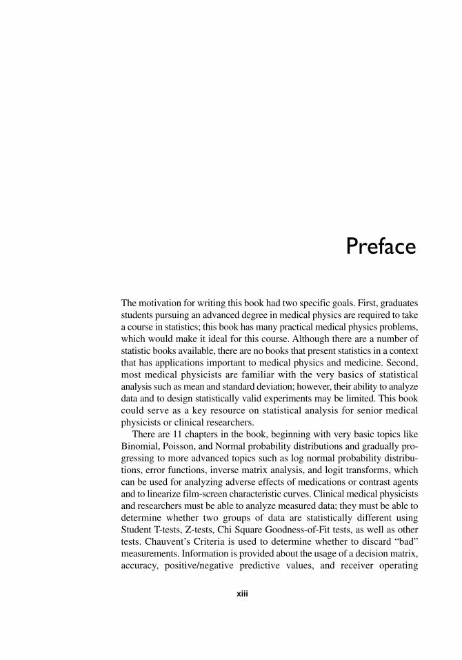
The motivation for writing this book had two specific goals. First, graduatesstudents pursuing an advanced degree in medical physics are required to takea course in statistics; this book has many practical medical physics problems,which would make it ideal for this course. Although there are a number ofstatistic books available, there are no books that present statistics in a contextthat has applications important to medical physics and medicine. Second,most medical physicists are familiar with the very basics of statisticalanalysis such as mean and standard deviation; however, their ability to analyzedata and to design statistically valid experiments may be limited. This bookcould serve as a key resource on statistical analysis for senior medicalphysicists or clinical researchers.

There are 11 chapters in the book, beginning with very basic topics likeBinomial, Poisson, and Normal probability distributions and gradually pro-gressing to more advanced topics such as log normal probability distribu-tions, error functions, inverse matrix analysis, and logit transforms, whichcan be used for analyzing adverse effects of medications or contrast agentsand to linearize film-screen characteristic curves. Clinical medical physicistsand researchers must be able to analyze measured data; they must be able todetermine whether two groups of data are statistically different using Student T-tests, Z-tests, Chi Square Goodness-of-Fit tests, as well as othertests. Chauvent’s Criteria is used to determine whether to discard “bad” measurements. Information is provided about the usage of a decision matrix,accuracy, positive/negative predictive values, and receiver operating

Preface

xiii

xiv ■ Preface

characteristic (ROC) curves. Chapter 5 on Bayes’ Theorem describes theinfluence of patient populations upon experimental results. Chapters 6 and 7 discuss, respectively, graphical data analysis, utilizing both linear andnonlinear functions, and correlation and the necessary design populationand correlation coefficient (R value) for experimental studies. Two chaptersintroduce the usage of fractals (chapter 8) and Monte Carlo methods in medicine (chapter 9). The most important chapter, chapter 10, uses simplestatistical methods to derive image analysis concepts like the signal-to-noiseratio (SNR), contrast-detail diagrams, detective quantum efficiency (DQE),and digital subtraction angiography (DSA). The last chapter discusses mis-use of statistics, covering topics such as spurious correlations, influence ofBayes’Theorem, systematic errors, improperly discarding unfavorable dataand other similar issues.

This book would make a valuable addition to any library due to the widerange of statistical topics and the many practical applications which areprovided throughout the text. While learning statistics, medical physicsgraduate students would benefit from a book which addresses practicalclinical topics rather than abstract statistical analysis, which is the approachof many other books on statistics.

8.1 BASIC CONCEPTS

Fractals are obtained by using a process whereby self-similar structuresare obtained from an object by adjusting the size of the object (eitherenlarging or minifying) by a specified magnification factor (R). Then,these self-similar objects are used to replace the original object or theyare added to the original figure at some particular location by a rule. Theprocess is then repeated many times. To illustrate this process, consider astraight line that is continuously reduced by half and used to replace theoriginal line (illustration 8.1).

163

8Fractals and Their Applications

Illustration 8.1

164 ■ Chapter 8

As the minification increases, the original line segment is replaced by a greater number of smaller line segments. The number of segments is designated “N”. The number of line segments (N) can be given by theequation that relates the original line length (L) and the magnification factor (R):

(8.1)

By taking a logarithm of both sides of the equation and rearranging theterms, equation (8.2) is obtained:

(8.2)

The symbol “D” is called the fractal dimension. To illustrate this calcula-tion, the fractal dimension (D) will be calculated for the third step shownin illustration 8.1. In this case, N = 8, R = 0.125, and L = 1.0.

(8.3)

Since this example deals with straight lines, it is not surprising that thefractal dimension is equal to one. Straight lines are one-dimensionalobjects in space.

Next, consider a square (see illustration 8.2). Again, envision the effectof using a magnification factor (R) equal to 0.5.

In this case, the original square is divided into four smaller squares. Thefractal dimension in this case is:

(8.4)

Again, the fractal dimension of 2.0 is consistent with the fact that a squareis a two-dimensional object.

Now, let us consider a cube that is replaced with cubes that are one-thirdthe original size (see illustration 8.3). The magnification factor (R) wouldbe 1/3.

DLog 4.0

Log 1.0 0.5

Log 4.0

Log 2.0=

( )( ) =

( )( ) = 2 0. .

DLog 8.0

Log 1.0 0.125

Log 8.0

Log 8.0=

( )( ) =

( )( ) = 1.00

DLog N

Log L R=

( )( ) .

N L RD= [ ] .

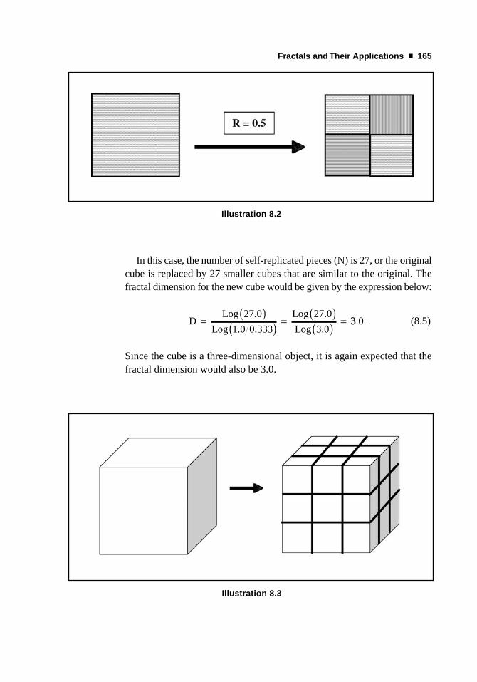
In this case, the number of self-replicated pieces (N) is 27, or the originalcube is replaced by 27 smaller cubes that are similar to the original. Thefractal dimension for the new cube would be given by the expression below:

(8.5)

Since the cube is a three-dimensional object, it is again expected that thefractal dimension would also be 3.0.

DLog 27.0

Log 1.0 0.333

Log 27.0

Log 3.0=

( )( ) =

( )( ) = 33 0. .

Fractals and Their Applications ■ 165

Illustration 8.2

Illustration 8.3

166 ■ Chapter 8

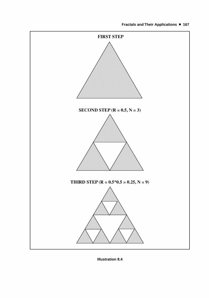
However, there are objects for which the fractal dimensions are not wholenumbers. One example is the Sierpinski triangle. The first step is to startwith an equilateral, shaded triangle. A rule for the formation of subsequentSierpinski triangles is to make inverted triangles of 0.5 the previous heightand 0.5 the previous width. These inverted triangles are placed internally ineach shaded triangle and are subtracted from the previous shaded triangles.This is illustrated in the figures in illustration 8.4.

In the second step, the original triangle becomes three smaller shadedtriangles by subtracting a half-width and half-height triangle, which isplaced inverted into the original triangle. In the third step, three smaller tri-angles are subtracted from the shaded triangles in step two. The remainingarea equals nine shaded triangles. For this series of triangles, the fractaldimensions in both step 2 and step 3 are shown in equation (8.6).

(8.6)

This fractal dimension is not a whole number. It has a dimension betweenone and two, and its numerical value is related to the complexity of thestructures that are formed by following the fractal rule.

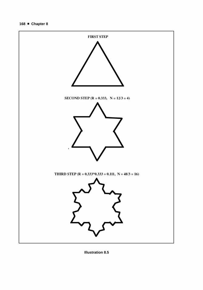
Another example also begins with a triangle (see illustration 8.5. Thereplication rule for self-similar objects is to divide each line segment intothree parts. Then the middle line segment is removed and replaced by twoline segments equal in length to the segment that is removed; these replace-ment line segments join in a point that looks like an added triangle. Theprocess can continue indefinitely forming what looks like a (Koch)snowflake.

For the second step, the line segments are divided into three equal segments, or R = 0.333. The number of line segments increases from 3 linesegments in the original triangle to 12; so N is equal to 12 divided by 3.For the third step, the line segments are divided into three again; R is equalto (1/3) multiplied by (1/3), or 0.111. The number of line segmentsincreases to 48; so N is equal to 48 divided by 3, or 16.

DLog 3.0

Log 1.0 0.5

Log 3.0

Log 2.0=

( )( ) =

( )( ) = 1 58. 55

1DLog 9.0

Log 1.0 0.25

Log 9.0

Log 4.0=

( )( ) =

( )( ) = ..585


Illustration 8.4

168 ■ Chapter 8

Illustration 8.5

For these series of figures, the fractal dimension is given below.

(8.7)

Again, for this fractal figure, the fractal dimension is not a whole numberthat relates to the complexity of the design pattern. Although line segmentswere the parameter evaluated for these fractal objects, the fractal dimensionis greater than 1.0, which is the normal value for a linear or line segmentobject.

There are many examples in nature for which the fractal dimension canbe computed, and these structures have different fractal dimensions thanregular geometric objects. The numerical value provides an index to thecomplexity of the object. For example, a tree consists of many repeatedbranches of its limbs, which could be analyzed by fractals.

8.2 EXAMPLES OF FRACTALS IN NATURE

Is there any practical application for these fractal concepts? Many objects innature and in medicine cannot be described by some simple combination ofrectangles, circles, cylinders, and spheres. The borders of real objects suchas trees, coastal shorelines, clouds, and many other objects in nature areragged and exhibit characteristics of fractal patterns when examined closely.Similarly, blood vessels in the human body, bronchi in the lungs, the EEGelectrical signals, and portions of the human central nervous system mightbe modeled by fractal patterns.

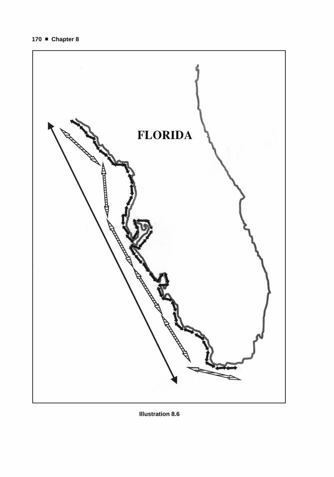
The published literature contains examples where fractals have been utilized to evaluate the complexity of the coastlines of various countries. Toillustrate this usage of fractals, we will examine the Florida coastline. Theresults depend upon the scale used to examine the shore. On a large scale,the shoreline may appear to be relatively smooth; however, by using asmaller unit of measurement, the complex nature of the coastline is betterrevealed. Illustration 8.6 shows a portion of the Florida coastline. The westcoastline of Florida on the figure is measured with different scale factors.

DLog 4.0

Log 1.0 0.333

Log 4.0

Log 3.0=

( )( ) =

( )( ) = 1.2262

DLog 16.0

Log 1.0 0.111

Log 16.0

Log 9.=

( )( ) =

( )00( ) = 1 262.


170 ■ Chapter 8

Illustration 8.6

By comparison to a single length measurement, the next smallest scale hasan R equal to 0.235 and N equal to 6. The smallest measurement scaleshown has an R value equal to 0.0353, and N equal to 41. In other words,the smallest scale of length shown fits 41 lines along the coastline whereasthe medium scale fits only 6 lines along the same coastline. As the scaleused to measure the coastline of Florida becomes smaller, more complexityin the variation of the shoreline is revealed. To evaluate this aspect of thecoast, the fractal dimension is calculated for the medium and small scalesshown on the map of Florida. For the medium scale measurement of theWest Florida coast, the fractal dimension is shown by equation (8.8).

(8.8)

For the smallest scale shown that is used to measure the length of thecoastline, the fractal dimension is even smaller; a smaller fractal dimensionindicates a smoother coastline.

(8.9)

The data for different size scales can be plotted in a graph with the abscissa“Log (L/R)” and the ordinate “Log (N)”, shown in illustration 8.7.

For this graph, the slope of the line is the estimated fractal dimension, D.The analysis of most coastlines in the published literature provides valuesbetween 1.02 for South Africa up to a value of 1.52 for the south coast ofNorway. By comparison, the Florida west coastline is relatively smooth witha low fractal dimension. The fractal dimension is a useful parameter for therelative comparison of the ruggedness of the various coastlines.

Another application of fractals in nature is the analysis of branchingstructures such as trees and rivers. Trees generally bifurcate many timesto produce their shape. With each change in the diameter of the branches(the scale factor), smaller and smaller branches are produced. However, areal tree is more complicated because it exists in three dimensions. Thesmall branches can be at various angles to the main branches; and the

DLog N

Log L R

Log 41

Log 1.0 0.0353

Log 41=

( )( ) =

( )( ) =

(( )( )

=

Log 28.33

D 1 111.

DLog N

Log L R

Log 6

Log 1.0 0.235

Log 6

L=

( )( ) =

( )( ) =

( )oog 4.255

D

( )

= 1 237.


172 ■ Chapter 8

smaller branches can be rotated at various angles around the main branch.Moreover, the branching is not always regular; there can be branches grow-ing at anomalous locations. Illustration 8.8 demonstrates the process ofbranching in a real tree. There are many different species of trees, and eachkind of tree may have its own branching pattern. Regardless, because ofthe self-replication of a generalized pattern, the branching of tree limbs canbe modeled by fractals, and it can be characterized by a specific fractaldimension.

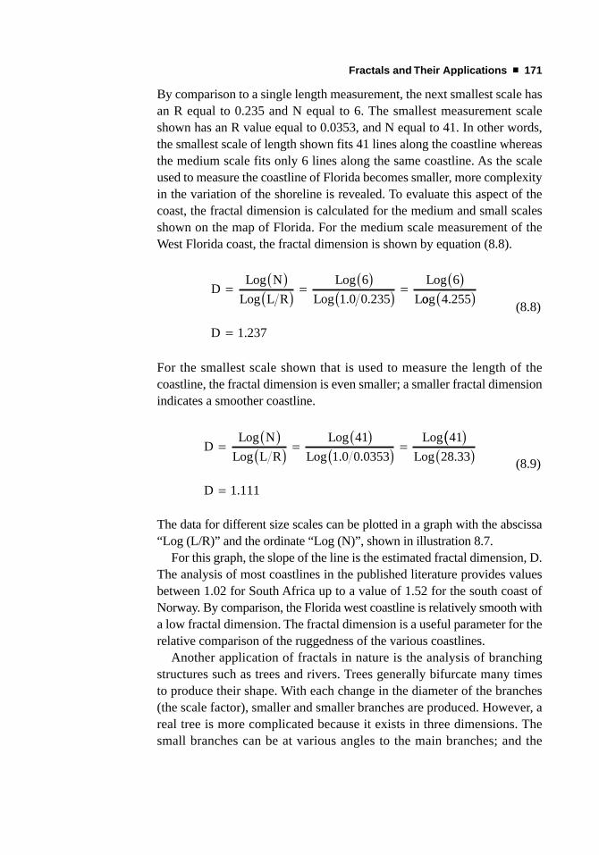
Three identical pictures are shown. On each picture, a grid is superim-posed with different size blocks on the grid. The size of the blocks of thevarious grids is related to the R factor of fractals. For each grid, the numberof blocks that contain a tree branch is counted; this number of blocks withobjects inside is related to the N value of the fractals. The “Log (N)” is plot-ted as a function of the “Log (R)”. The slope is the fractal dimension, D.This method is called the box counting method of fractal analysis.

Illustration 8.7


Illustration 8.8a

Illustration 8.8b

174 ■ Chapter 8

Illustration 8.8c

Illustration 8.9

As the slope on the graph in illustration 8.9 demonstrates, the fractaldimension for this particular example is about 1.40.

Branching of tree limbs has similar analogies in anatomy. The branchingof the airways in the lungs, the branching of veins and the arterial systemsin the human body, and nerves in the nervous system could be analyzed byusing fractal dimensions. One motivation for examining human anatomyby using fractals is that abnormalities in between segments of organs andbetween individuals might be uncovered with better speed, accuracy, andconsistency than by using conventional methods.

8.3 APPLICATIONS OF FRACTALS TO HUMAN ANATOMY

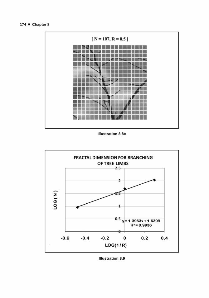
The branching of airways in the lungs is a self-replicating process, whichis similar to the branching of trees. See illustration 8.10 for an example ofthis process.

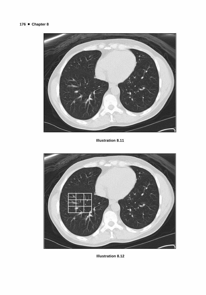
The best clinical image of the lungs is provided by a CT scanner in whicha lung display window and level is used. This is shown in illustration 8.11.

There are two different methods to determine the fractal dimensions fromthe data in the lung CT scan. The first method is to use the box countingapproach that was used in the example with tree branches. In this case, somecriteria must be utilized to determine whether or not a box gets counted. The


Illustration 8.10. Branching in bronchi of lungs, which looks like fractals.

176 ■ Chapter 8

Illustration 8.11

Illustration 8.12


observer needs to select a CT number threshold for the counting criteria.For this example, any box which had an average CT number in the regionof interest greater than –800 Hounsfield Units (H.U.) was counted. Boxeswith the average CT number inside the box of less than −800 H.U. werenot counted. This process is shown in illustration 8.12.

The problem with this approach is that the lung values vary with locationwithin the lung and from one CT slice to the other. A detailed analysiswould evaluate each section of the lung and each CT slice. For the purposesof this example, the data from the regions shown were measured and plot-ted as a graph of Log (N) versus Log (1/ R) in illustration 8.13.

From the box counting approach, the fractal dimension of the lungregion in the given CT slice is the slope of the graph (trend line), or 1.953.

Another approach would be to measure the mass in a series of concentriccircles in the same location. Circular regions of interest can be easily deter-mined from the CT scanner data. The area of the circular regions of interestcan be used to find the radii of the concentric circles:

Illustration 8.13

178 ■ Chapter 8

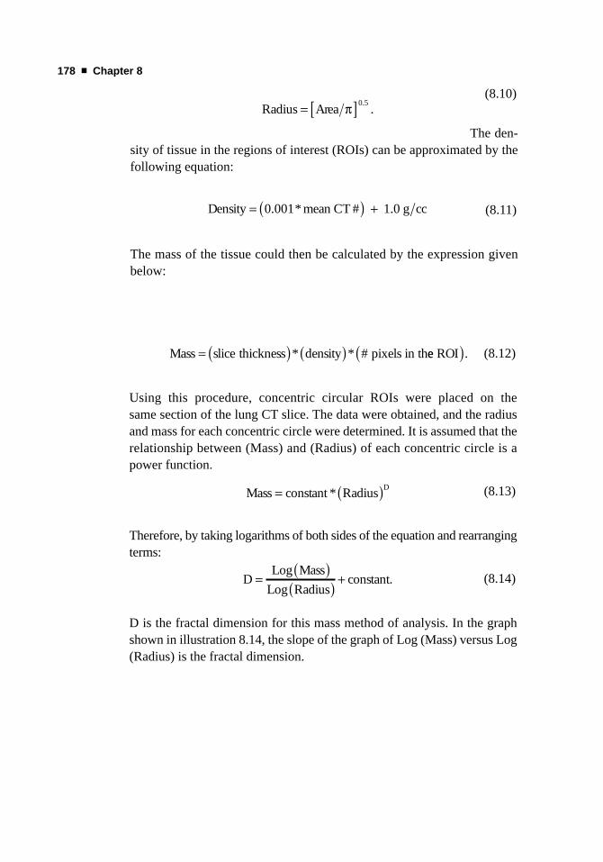
(8.12)

Using this procedure, concentric circular ROIs were placed on the same section of the lung CT slice. The data were obtained, and the radiusand mass for each concentric circle were determined. It is assumed that therelationship between (Mass) and (Radius) of each concentric circle is apower function.

(8.13)

Therefore, by taking logarithms of both sides of the equation and rearrangingterms:

(8.14)

D is the fractal dimension for this mass method of analysis. In the graphshown in illustration 8.14, the slope of the graph of Log (Mass) versus Log(Radius) is the fractal dimension.

DLog Mass

Log Radiusconstant.=

( )( ) +

Mass constant RadiusD= ( )*

Mass slice thickness density # pixels in th= ( ) ( )* * ee ROI( ).

(8.10)

The den-sity of tissue in the regions of interest (ROIs) can be approximated by thefollowing equation:

(8.11)

The mass of the tissue could then be calculated by the expression givenbelow:

Density mean CT g cc= ( ) +0 001 1 0. * # .

Radius Area= [ ]π 0 5..

Slightly different fractal dimensions are obtained by the two methods.Regardless, a value of about 2.0 for the fractal dimension indicates thebranching structure of the vessels occupies much of the space for the tissuein the lungs. This type of analysis can be used for other anatomical structuresin the body.

8.4 MANDELBROT SETS

To continue with the topic of self-replicating figures, mathematical processescan produce graphs with patterns. Standard polynomials only generate graphsof various continuous curves. However, by using complex numbers, moreinteresting figures can be generated. A complex number has a real number,which is plotted along the abscissa (x-axis), and an imaginary number, whichis plotted along the ordinate (y-axis). The square root of −1.0 is an imaginarynumber that is given the symbol i. Hence, a complex number can be writtenin the following form:


Illustration 8.14

180 ■ Chapter 8

(8.15)

A sequence of complex numbers is generated from a starting complex poly-nomial. The number that is computed is then substituted into the originalcomplex polynomial, and the process is continued many times. Mathemati-cally, the process can be written as the following expression:

(8.16)

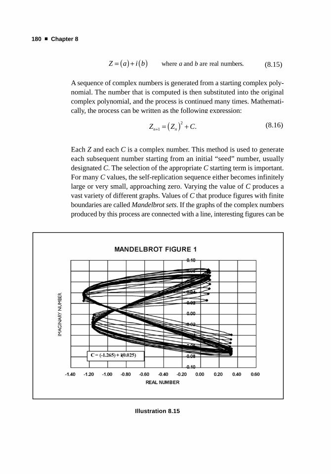
Each Z and each C is a complex number. This method is used to generateeach subsequent number starting from an initial “seed” number, usuallydesignated C. The selection of the appropriate C starting term is important.For many C values, the self-replication sequence either becomes infinitelylarge or very small, approaching zero. Varying the value of C produces avast variety of different graphs. Values of C that produce figures with finiteboundaries are called Mandelbrot sets. If the graphs of the complex numbersproduced by this process are connected with a line, interesting figures can be

Z Z Cn n+ = ( ) +1

2.

Z a i b a b= ( ) + ( ) where and are real numbers.

Illustration 8.15


Illustration 8.16

Illustration 8.17

182 ■ Chapter 8

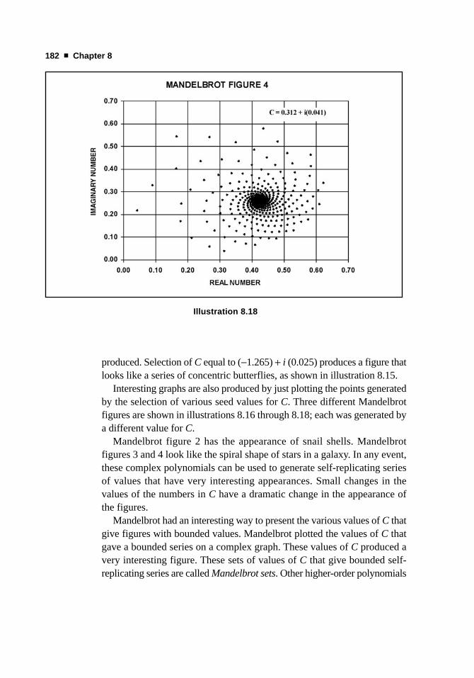
produced. Selection of C equal to (−1.265) + i (0.025) produces a figure thatlooks like a series of concentric butterflies, as shown in illustration 8.15.

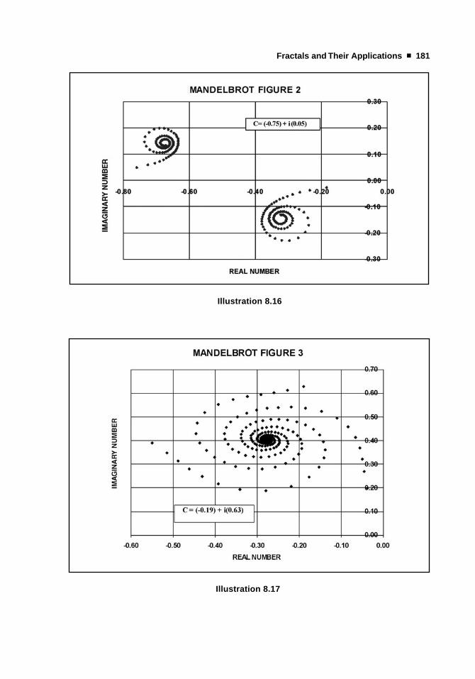
Interesting graphs are also produced by just plotting the points generatedby the selection of various seed values for C. Three different Mandelbrotfigures are shown in illustrations 8.16 through 8.18; each was generated bya different value for C.

Mandelbrot figure 2 has the appearance of snail shells. Mandelbrot figures 3 and 4 look like the spiral shape of stars in a galaxy. In any event,these complex polynomials can be used to generate self-replicating seriesof values that have very interesting appearances. Small changes in the values of the numbers in C have a dramatic change in the appearance ofthe figures.

Mandelbrot had an interesting way to present the various values of C thatgive figures with bounded values. Mandelbrot plotted the values of C thatgave a bounded series on a complex graph. These values of C produced avery interesting figure. These sets of values of C that give bounded self-replicating series are called Mandelbrot sets. Other higher-order polynomials

Illustration 8.18

can also be used to generate interesting figures and their seed values of C canalso be plotted as a graph.

USEFUL REFERENCES

Barnsley, M. F. Fractals Everywhere, 2nd edition. San Diego, CA: Academic

Press, 2000.

Briggs, J. Fractals: The Pattern of Chaos: Discovering a New Aesthetic of Art,

Science and Nature. New York: Simon & Schuster, 1992.

Falconer, K. J. Techniques in Fractal Geometry. West Sussex, England: John

Wiley & Sons Ltd., 1997.

Falconer, K. J. Fractal Geometry: Mathematical Foundations and Applications.

West Sussex, England: John Wiley & Sons Ltd., 2003.

Gleick, J. Chaos: Making a New Science, 2nd edition. New York: Penguin

Books, 2008.

Leibovitch, L. S. Fractals and Chaos: Simplified for Life Sciences. New York:

Oxford University Press, Inc., 1988.

Mandelbrot, B. B. The Fractal Geometry of Nature. New York: W. H. Freeman, 1983.

Mandelbrot, B. B. Fractals and Chaos: The Mandelbrot Set and Beyond. New

York: Springer-Verlag New York Inc., 2004.

Peterson, I. The Mathematical Tourist: New and Updated Snapshots of Modern

Mathematics. New York: Barnes & Noble Books, 2001.

Schroeder, M. Fractals, Chaos, Power Laws: Minutes from an Infinite Paradise.

Mineola, NY: Dover Publications, 2009.

PRACTICE EXERCISES

1. On a square, divide each side into three parts. On each center segment,add another square that has sides that are one-third the length of theoriginal square. Repeat this process two more times. What is the areaencompassed by the new figure? How many line segments are on thecircumference of the new figure? How does the length of circumfer-


184 ■ Chapter 8

ence of the new figure compare with the original figure? What is itsfractal dimension?

2. Obtain a picture of a tree that has lost its leaves. Use the box count-ing method to determine it fractal dimension. What is this value ofthe fractal dimension? Is this a value that you would expect?

3. Obtain a picture of the coastline of Ireland. Use the box countingmethod to determine its fractal dimension. Try to find an article thatcomputes Ireland’s fractal dimension. How well do the calculationscompare with the published value? If the coastline is more complex,does the fractal dimension increase or decrease? Why is this important?

4. Obtain a picture of the venous blood vessels in the leg. Use the boxcounting approach to determine the fractal dimensions. What is themathematical description of the repetition pattern of the branching?Why is this important? If the value of the fractal dimension decreases,what does it mean from a physiological viewpoint?

5. Obtain a CT scan image with a slice through the kidneys that can beanalyzed for its CT numbers. Use the density approach described inthis book to determine its fractal dimensions. What is this fractaldimension? If the value is found to be greater in other patients, whatdoes this indicate clinically?

6. Create a graph of a Mandelbrot set using the starting value of C = (−0.25) + (0.96) i. Continue the process through at least 100terms. Plot the points and connect the points with lines. Change thevalues for C slightly to obtain another figure.

7. Create a picture of a tree by using a repeating branching processwhere the braches are one-half the length of the original tree trunk.What is the mathematical description of the branching process thatwas used? How might the tree be made more realistic?

8. Create a sequence of numbers using a polynomial feedback loop ofXn+1 = K* Xn * (1 − Xn) where K is a constant. Let K = 1.15 and let thestarting value of X0 = 0.11. Plot Xn+1 on the ordinate axis versus Xn onthe abscissa axis. Describe the appearance of the graph. Does thegraph have a maximum? Is there anything in the medical or medicalphysics worlds that could be described with a feedback loop?

9. Create an interesting image starting with a rectangle and using a rule inwhich smaller rectangles are subtracted from the original rectangle.Describe the rule in detail. Provide the image of the resultant figureafter five iterations. If the process were to continue infinitely, whatwould be the area remaining from the original figure? What would bethe number of line segments used to form the figure? What would bethe fractal dimension?

10. Explain how fractals might be useful in other sciences like astronomy,zoology, and chemistry. Give a detailed example. What is the overallbenefit of fractals? How does the universe look from a small-scaleprospective?


Index

accuracy of a test, 80activity of a radioisotope, 21, 128–131,

129f, 129t, 130f, 131fambiguous survey data, 245appointment schedules, 198–202, 199f,

200f, 201f, 202fattenuation coefficient, linear, 205–206,

205f, 206tAutomatic Exposure Control (AEC), 125average. See central tendency; mean

Bayes’ Theorem, 97–108applications of, 103–108

to cancer risk from CT, 106–108to drug testing, 103–104, 244to mammography screening,

104–105basic concepts of, 97–99population characteristics and, 99–102,

100f, 102f, 244bell curve. See Normal (Gaussian)

probability distributionbiased sampling, 240–241, 243bi-modal frequency distribution, 7binomial probability distribution, 18–25

applications ofto CT scanner downtime, 22–23, 23fto isotopic decay, 22, 24–25, 25fto mammography screening, 23–24

fundamentals of, 18–22, 20f, 20t, 21fmean of, 26

Poisson distribution and, 25–26blood pressure measurements

Chi-Square Test with, 88dividing into two groups, 76–78, 77f,

79f, 80ROC graph for, 82, 83f, 83t, 84

in flawed experiments, 240–241,245–246

blur, 222, 223f, 224–225, 226, 227box counting method of fractal analysis,

172, 173f, 174ffor lung CT, 175, 176f, 177, 177fbranching structures, fractal analysis of,

171–172, 173f, 174f, 175

calibrationerrors in, 245–246of ionization chambers, 90–92, 91t

cataracts, radiation-induced, 43–44causation, fallacious inference of,

155–156, 156f, 240, 241f, 244central tendency, 6–7, 17. See also mean;

median; modeinappropriate use of, 238–239, 238f,

239fcentral two-tailed cumulative probability,

60, 61f. See also two-tailedcumulative probability distribution

characteristic curve, for film-screensystems, 43, 66, 67–68, 69f, 70

Chauvenet’s criterion, 87–88, 88t

275

Note: Page numbers followed by f refer to figures; page numbers followed by t refer to tables.

chest imagingfractal analysis of, 175–178, 175f, 176f,

177f, 179fnoise in, 216f

Chi-Square Test, 88–90, 89f, 90tcluster sampling, 51CNR. See contrast-to-noise ratio (CNR)coastlines, fractal, 169, 170f, 171, 172fCoefficient of Alienation, 155Coefficient of Determination, 155Coefficient of Non-Determination, 155coherent scatter, 204f, 205–207, 206t, 207fcoin toss, 18–21, 20f, 20t, 21fcollisions, molecular, 190, 191–192combinations, 2–4, 3f, 4tcomplementary error function (ERFC), 41complex numbers

defined, 179iterated sequences of, 179–182, 180f,

181f, 182fCompton scatter, 204f, 205–210, 206t,

207fangular dependence, 207–209, 208f,

209fphoton energy, 208–209

computed radiography (CR), noise in, 216fcomputed tomography. See CT (computed

tomography)conditional probability, 97–99. See also

Bayes’ Theoremconfidence intervals, 60, 64–66, 65f, 65t

applications ofto CT radiation dose, 92–93to mammography radiation dose,

70–71for linear regression, 137–138, 140, 141ffor mean value, 66, 70, 76with one-tailed distribution, 66, 71in quality control, 246

confounding factors, 241, 244continuous frequency distribution, 5contrast agent, in digital subtraction

angiography, 227–232, 229f, 230fcontrast agent toxicity

Chi-Square Test for age hypothesis, 89–90, 90t

Log Normal distribution of, 37–38, 37t,38f, 66

contrast-detail diagrams, 220–225, 222fcontrast-to-noise ratio (CNR), 217–220,

218f, 219fblur and, 222, 224–225in digital subtraction angiography,

228–232size of low-contrast object and, 221,

225control group, 240–241correlation

for linear functions. See correlationcoefficient

for nonlinear functions, 157spurious, 155–156, 156f, 240, 241f,

244correlation coefficient, 149–151

alternative form for, 151–153application of, 153, 154–155causal relationship and, 155–156, 156f,

240, 241fsignificance of, 153–155table for, 269–273terminology for, 155TC test for, 153–154, 155, 270

CR (computed radiography), noise in, 216fCT (computed tomography)

blur in, 222lung, fractal analysis of, 175–178, 175f,

176f, 177f, 179fradiation dose from

cancer caused by, 106–108, 243confidence limits for, 92–93to head, 32–34, 33f, 33t, 34f,

106–107number of measurements, 86–87

scanner downtime, 22–23, 23fsignal-to-noise ratio in, 216–217

CTDI (computed tomography dose index),32–34, 33f, 33t, 34f

cancer risk and, 106confidence limits for, 92–93number of measurements, 86–87

cumulative frequency distribution, 7–8, 8fcumulative probability distributions. See

Log Normal probability distribution,cumulative; Normal (Gaussian)probability distribution, cumulative;one-tailed cumulative probability

276 ■ Index

distribution; two-tailed cumulativeprobability distribution

curve fitting. See least squares method

decay constant, 21, 24decay rate, 21–22, 24–25, 25fdecision matrix, 77–81, 78t, 79t, 80t

in Bayesian analysis, 99, 103, 107degrees of freedom (df)

Chi-Square Test and, 89, 89f, 90T-test and, 85, 265–267

Detective Quantum Efficiency (DQE),225–227

digital imaging systems. See also imagequality

signal-to-noise ratio of, 216f, 217digital subtraction angiography (DSA),

227–232, 229f, 230f, 232f, 233fdiscarding data, 87–88, 88t, 241, 244–245discrete frequency distribution, 4t, 5, 5fdispersion of probability distribution, 17,

17f. See also standard deviation (SDor σ)

distributions. See frequency distributions;probability distributions

dose. See contrast agent toxicity; radiationdose

downtime, CT scanner, 22–23, 23fDQE. See Detective Quantum Efficiency

(DQE)drug screening, 103–104, 244DSA. See digital subtraction angiography

(DSA)

edge enhancement algorithms, 215efficiency of image receptor, 225–226electronic components

cluster sampling of, 51cumulative failure of, 43time to failure of, 35, 36f

electronic noise, 190–191, 191f, 215, 226equally likely outcomes, 13, 14fERFC (complementary error function), 41Error Function (ERF), 38–43, 41f, 43f, 60.

See also Normal (Gaussian)probability distribution, cumulative

applied to cataract risk, 43–44table of, 255–257

Excel spreadsheetChi-Square Test with, 89of head CT radiation doses, 33–34, 34frandom number generator of, 188, 189f,

190, 194T-test with, 85

experiments, poorly designed, 240–242,244–245

exponential functions, 127–131correlation for, 157least squares fitting with, 130, 132logarithmic functions and, 132processes represented by, 127

exposure from x-ray tube, 57–59, 58t, 59t,70

factorialsgamma function and, 265Stirling approximation to, 27

False Negatives (FN), 78–81, 79f, 79t, 80tconditional probability and, 97, 99

False Positives (FP), 78–81, 79f, 79t, 80tconditional probability and, 97, 99ROC graphs and, 82–84, 83f, 83t

fences, 64–66, 65f. See also confidenceintervals

film-screen systemscharacteristic curve for, 43, 66, 67–68,

69f, 70signal-to-noise ratio of, 216–217

flood-field image, 220fourth moment of probability distribution,

16fractal dimension, 164–166, 169

by box counting method, 172, 173f, 174ffractals

applications ofto branching structures, 171–172,

173f, 174f, 175to coastlines, 169, 170f, 171, 172fto lung CT, 175–178, 175f, 176f,

177f, 179fbasic concepts of, 163–169, 163f, 165f

frequency distributions, 4–6, 4t, 5f, 6fbi-modal, 7cumulative, 7–8, 8fmeasures of central tendency for, 6–7

full width at half maximum (FWHM), 30

Index ■ 277

gamma function, 265Gaussian distribution. See Normal

(Gaussian) probability distributionGeiger-Mueller detector, 27–29, 28f, 29f,

29tGolden Ratio, 117–119, 117t, 118fgoodness of fit, Chi-Square Test for,

88–90, 89f, 90tgrades of students, distribution of, 31–32,

32tgraphical fits to data. See least squares

method

half-life, of radioisotope, 21, 24height vs. age of boys

correlation coefficient for, 153, 154–155linear regression of, 138–140, 138t,

139t, 141fhistogram, 4, 5fhypothesis testing, with Chi-Square Test,

88–90, 89f, 90t

identity matrix, 121image processing, 215image quality

blur, 217, 222, 223f, 224–225, 226, 227contrast-to-noise ratio, 217–220, 218f,

219f, 221, 222, 224–225in digital angiography, 228–232

Detective Quantum Efficiency (DQE), 225–227

Noise Equivalent Quanta (NEQ), 226, 227

radiation dose and, 216–217, 227signal-to-noise ratio, 215–217, 216f,

225–227in digital angiography, 228–229,

231–232size of low-contrast objects and,

220–222, 222f, 225sources of noise, 215, 226–227

Index of Correlation, 157intensifying screens. See film-screen

systemsinverse matrix

calculation of, 121–122in linear regression, 119–123

in second-degree curve fitting, 125–126ionization chambers, calibration of, 90–92,

91t

Koch snowflake, 166, 168f, 169Kurtosis, 16–17

least squares method. See also linearregression

for linear fit, 112–119with exponential data, 130, 132with logarithmic data, 132with power function, 135using inverse matrix, 119–123

for polynomial fit, 123–126, 125t, 127fleptokurtic distribution, 17linear attenuation coefficient, 205–206,

205f, 206tlinear correlation coefficient. See

correlation coefficientlinear regression. See also correlation

coefficient; least squares method;standard error of the estimate (SE)

basic concepts of, 111–119confidence intervals for, 137–138, 140,

141fexample of Golden Ratio, 117–119,

117t, 118ffor exponential data, 128, 130–131,

130f, 131f, 132inverse matrix approach to, 119–123for logarithmic data, 131–132

line spread function (LSF), 224logarithmic functions, 131–132

correlation for, 157Logit Transform, 66–70, 69flog-log graph, 132–133

application of, 133–135, 133t, 134fLog Normal probability distribution

applied to toxicities, 37–38, 37t, 38f, 66, 67, 68f

cumulative, 66, 67, 68ffundamentals of, 34–36, 36f

lower one-tailed cumulative probabilitydistribution, 42–43, 42f, 43f, 60, 61f

applied to cataract risk, 44sigmoid curves and, 43, 43f, 66

278 ■ Index

table of values, 259–263LSF (line spread function), 224lung CT, fractal analysis of, 175–178,

175f, 176f, 177f, 179f

mammographyaverage glandular dose, 70–71, 92,

124–126, 125t, 127fscreening with, 23–24, 79, 104–105

Mandelbrot sets, 179–182, 180f, 181f,182f

mask, angiographic, 228, 230, 230f, 231,232, 233f

mass attenuation coefficients, 204f,205–206, 206t

matrix multiplication, 119–120mean, 6–7. See also standard error of the

mean (SE)of binomial distribution, 26inappropriate use of, 238, 239, 239fof Normal distribution, 29–30, 49–50, 53tof Poisson distribution, 26–27, 53–54of population, 30, 51, 52of sample, 30, 51–52

sample size and, 52, 86–87, 92, 196–198, 197f, 197t

variation of, 75–76of skewed probability distribution, 14,

15, 16weighted, 50

median, 6, 7, 8inappropriate use of, 238–239, 238fof Normal distribution, 49of skewed probability distribution, 14,

15, 16mesokurtic distribution, 17mining data, 245misuse of statistics, 237–246

categories of, 242–246introduction to, 237–242, 242f

mode, 6, 7dispersion and, 17of Normal distribution, 49of skewed probability distribution, 14,

15, 16modulation transfer function (MTF),

224–225, 226, 227

molecular collisions, 190, 191–192Monte Carlo methods

applications ofmean value variation, 196–198, 197f,

197tscheduling appointments, 198–202,

199f, 200f, 201f, 202fx-ray photon interactions, 203–210

basic process in, 192, 194–196, 195frandom numbers for, 187–190, 189ftrials (histories) in, 196

Negative Predictive Value (NPV), 81noise. See contrast-to-noise ratio (CNR);

electronic noise; image quality;quantum mottle; signal-to-noise ratio(SNR)

Noise Equivalent Quanta (NEQ), 226, 227Normal (Gaussian) probability distribution

Chauvenet’s criterion and, 88cumulative, 38–43, 40f, 41f, 42f, 43f

approximation to, 62–63, 63t, 64fconfidence intervals and, 60, 64–66,

65f, 65t, 71, 76four types of, 60, 61f, 62fin Monte Carlo method, 194–196,

195f, 200table of values, 255–257Z value and, 84–85, 85t

fundamentals of, 29–31, 31fimage contrast and, 219, 219fmean of, 29–30, 49–50, 53tquestionable applications of

to head CT radiation dose, 32–34, 33f, 33t, 34f

to student grades, 31–32, 32tseparation of two populations, 76–77,

77fZ parameter and, 84–85, 85t, 91

skewed example compared to, 32–34, 33f, 34f

standard deviation of, 29, 30–31, 31f, 50–51, 52, 53t

confidence intervals and, 64–66, 65f, 65t

cumulative probability and, 62–63, 63t, 64f

Index ■ 279

Normal (Gaussian) probability distribution(continued)

table of values, 249–254T distribution compared to, 85, 266, 269variance of, 50–51, 53t

nuclear medicine. See also radioactivedecay

contrast-to-noise ratio in, 220quantum mottle in, 216signal-to-noise ratio in, 71

one-tailed cumulative probabilitydistribution, 41–43, 42f, 43f, 60, 61f,

62fapplied to cataract risk, 44confidence level for, 66, 71in random number generation, 195sigmoid curves and, 43, 43f, 66, 195table of values, 259–263T-test and, 86, 267Z value and, 84

optical transfer function (OTF), 224

peakedness of probability distributions,16–17

permutations, 1–2, 2f, 3, 3f, 4tphotoelectric effect, 204f, 205–207, 206t,

207fpixel shifting, 228platykurtic distribution, 17Poisson probability distribution, 25–29

Chauvenet’s criterion and, 87fundamentals of, 25–27Geiger-Mueller detector and, 27–29,

28f, 29f, 29tmean of, 26–27, 53–54standard deviation of, 52–54

polynomial fit to data, 123–126Index of Correlation for, 157

population. See also separation of twopopulations

mean of, 30, 51, 52standard deviation of, 30, 51, 52

Positive Predictive Value (PPV), 81power functions, 132–133

application of, 133–135, 133t, 134fcorrelation for, 157

probability distributions, 13–17. See alsobinomial probability distribution;cumulative probability distributions;Log Normal probability distribution;Normal (Gaussian) probabilitydistribution; Poisson probabilitydistribution; skewed probabilitydistributions; T distribution

product moment coefficient, 150

quality control, confidence intervals in,246

quality of image. See image qualityquantum mottle, 215, 216, 226

in digital subtraction angiography, 228, 229f, 230

quartile deviation (QD), 16quartiles, 7, 8questionnaires, poorly designed, 246

radiation detector, Geiger-Mueller, 27–29,28f, 29f, 29t

radiation doseambiguous survey of, 245from CT scans

cancer caused by, 106–108, 243confidence limits for, 92–93to head, 32–34, 33f, 33t, 34f,

106–107number of measurements of, 86–87

cumulative probability of bioeffect, 42image quality and, 216–217, 227to laboratory workers’ thyroids, 56, 86to lens of eye, 43–44in mammography, 70–71, 92, 124–126,

125t, 127fMonte Carlo calculations of, 203, 210whole-body, 66

radiation exposure from x-ray tube, 57–59,58t, 59t, 70

radioactive decay, 21–22, 24–25, 25fgraphical fit to data, 127–131, 129f,

129t, 130f, 131fscintillation counter and, 54–55, 54t

RAND( ), 188, 189f, 190, 194random numbers, 187–190, 189frandom sampling, 51

280 ■ Index

random walk, 190–192, 191f, 193f, 194fReceiver Operating Characteristic (ROC)

graphs, 82–84, 83frelative frequency distribution, 5–6, 6f

cumulative, 7–8, 8fmeasures of central tendency, 6–7

weighted mean, 50relative standard deviation (RSD), 54–55,

54t

samplediscarding data from, 87–88, 88t, 241representative of population, 75–76

sample mean, 30, 51–52. See also standarderror of the mean (SE)

sample size and, 52, 86–87, 196–198, 197f, 197t

variation of, 75–76sampling, 51–52sampling error, 240–241, 243scattered radiation

coherent, 204f, 205–207, 206t, 207fCompton scatter, 204f, 205–210, 206t,

207fangular dependence, 207–209, 208f,

209fphoton energy, 208–209

scheduling appointments, 198–202, 199f,200f, 201f, 202f

scintillation camera, flood-field imagewith, 220

scintillation counter, standard deviationfor, 54–55, 54t

SD. See standard deviation (SD or σ)SE. See standard error of the estimate (SE);

standard error of the mean (SE)semilogarithmic graph, 128, 130–131,

130f, 131f, 132sensitivity of a test, 80, 99–100, 101, 102,

244separation of two populations, 76–77, 77f

applications of, 90–93, 91tdecision matrix and, 77–81, 78t, 79t, 80tROC graphs and, 82–84, 83fT-test for, 84–86

application of, 90–92, 91ttable of values, 265–267

Z parameter and, 84–85, 85tSierpinski triangle, 166, 167fsigmoid curves, 43, 43f, 66

Logit Transform and, 66–70, 68f, 69fin random number generation, 195

signal-to-noise ratio (SNR), 71–72,215–217, 216f

Detective Quantum Efficiency and, 225–227

in digital subtraction angiography, 228–229, 231–232

skewed probability distributions, 14, 14f,15–16, 15f

inappropriate analysis of, 238–239, 238f

Log Normal. See Log Normalprobability distribution vs. Normaldistribution, 32–34, 33f, 34f

skewness, 16, 34fsmoothing algorithms, 215snowflake, 166, 168f, 169spatial frequency of image, 224–225, 227specificity of a test, 81, 99, 101, 102, 244standard deviation (SD or σ), 17

for added or subtracted data, 55–56, 55finappropriate use of, 238for multiplied or divided data, 56–58,

58t, 59tof Normal distribution, 29, 30–31, 31f,

50–51, 52, 53tconfidence intervals and, 64–66, 65f,

65tcumulative probability and, 62–63,

63t, 64fof Poisson distribution, 52–54relative, 54–55, 54tof sample vs. population, 30, 51, 52skewness in terms of, 16

standard error of the estimate (SE),135–138

application of, 138–140, 138t, 139t, 141f

correlation coefficient in terms of, 152standard error of the mean (SE), 59, 75–76

confidence levels for, 66, 70with Monte Carlo method, 196–198,

197f

Index ■ 281

standard error of the mean (SE), 59, 75–76(continued)

Student’s T-test and, 84–86Z values and, 84–85, 86

standard error of Y, for nonlinear fit todata, 157

statisticsbeneficial uses of, 246misuse of, 237–246

Stirling approximation, 27stratified sampling, 51Student’s T-test. See T-testsurveys, poorly designed, 245, 246symmetrical probability distribution, 15,

15f, 16systematic measurement errors, 241,

245–246systematic sampling, 52

T distribution, 265–266tolerances, 60. See also confidence

intervalstoxicities, Log Normal distribution of,

37–38, 37t, 38f, 66, 67, 68fTrue Negatives (TN), 78–81, 79f, 79t, 80t

conditional probability and, 97True Positives (TP), 78–81, 79f, 79t, 80t

conditional probability and, 97ROC graphs and, 82–84, 83f, 83t

T-test, 84–86for ionization chamber calibration,

90–92, 91ttable of values, 265–267

TC test for correlation coefficient,153–154, 155, 270

two-tailed cumulative probabilitydistribution, 20–21, 21f, 60, 61f

confidence intervals for, 64–66, 65f, 65tError Function as, 39–41, 41fPoisson, 29, 29f, 29tin random number generation, 194–196,

195f

table of values, Normal, 255–257T-test and, 85, 266Z value and, 84

unsharpness. See blurupper one-tailed cumulative probability

distribution, 60, 62fconfidence level for, 66, 71

variance (σ2)of Normal distribution, 50–51, 53tof Poisson distribution, 53

waiting times, 198–202, 199f, 200f, 201f,202f

weighted mean, 50weighting factor, 50well scintillation counter, standard

deviation for, 54–55, 54twhite noise, 216Wiener Noise, 227

x-ray film-screen systems. See also imagequality

characteristic curve for, 43, 66, 67–68, 69f, 70

signal-to-noise ratio of, 216–217x-ray imaging

contrast-to-noise ratio in, 220signal-to-noise ratio in, 216–217, 216f

x-ray photon interactions, 203–210x-ray tube

energy spectrum of, 203, 204fexposure from, 57–59, 58t, 59t, 70focal spot blur with, 222output vs. kVp, 133–135, 133t, 134freproducibility assessment of, 52, 53t,

70

Z parameter, 84–85, 85t, 86–87correlation coefficient and, 153–154

282 ■ Index

Dr. Edward L. Nickoloff completed his B.S. degree in Physics from LebanonValley College in Annville, Pennsylvania, and his M.S. degree in NuclearPhysics from the University of New Hampshire in Durham, New Hampshire.After his M.S. degree, Dr. Nickoloff worked in the electronic industry for 6 years. Then, due to the death of his mother Pearl from cancer, he wanted towork and do research in the medical field. To pursue this goal, he returned tograduate school; he received his D.S. degree with Distinction in MedicalPhysics from Johns Hopkins University, Baltimore, Maryland. Even prior tograduation, Dr. Nickoloff was hired by the Department of Radiology at theJohns Hopkins Medical Institutions as an Assistant Professor of Radiologyand Acting Director of Physics and Engineering. Subsequently, he wasrecruited to the Department of Radiology at Columbia University and theColumbia University Medical Center of the New York-Presbyterian Hospital.Dr. Nickoloff advanced professionally to the academic title of Professor ofRadiology and appointment as Chief Hospital Physicist. Dr. Nickoloff isboard certified in Diagnostic Radiology Physics and Nuclear MedicinePhysics by the American Board of Radiology (ABR), in Diagnostic ImagingPhysics by the American Board of Medical Physics (ABMP) and in HealthPhysics by the American Board of Health Physics (ABHP). He has served asPresident of the Radiological and Medical Physics Society of New York(RAMPS, Inc.), Chairman of the American College of Medical Physics

283

About the Author

284 ■ About the Author

(ACMP), Treasurer and Chair of examination panels for the ABMP, andSecretary of the Greater New York Chapter of Health Physics Society(GNYCHPS). He has served on the Board of Directors for the AmericanAssociation of Physicists in Medicine (AAPM), ACMP and ABMP. Dr. Nickoloff has published 2 books, about 30 book chapters, 55 peer-reviewed journal articles, about 70 journal abstracts; his book entitled Radiology Review: Radiologic Physics is used by many programs trainingradiology residents. In addition, he has given over 130 presentations at professional meetings. He has been honored by being awarded the title ofFellow by the American College of Radiology (FACR), American Collegeof Medical Physics (FACMP) and the American Association of Physicistsin Medicine (FAAPM). He has been an active member in numerous pro-fessional organizations. Dr. Nickoloff was also honored for his lifetimeachievements by the ACMP, as a recipient of the Marvin M.D. WilliamsAward. Dr. Nickoloff is still very active in medical physics, and he teachesRadiology residents and Applied Physics graduate students at ColumbiaUniversity.

applications of statistics to medicine and medical physics

Documents