San Jose State University San Jose State University

SJSU ScholarWorks SJSU ScholarWorks

Master's Theses Master's Theses and Graduate Research

Fall 2018

Application of Model Predictive Control in Modular Multilevel Application of Model Predictive Control in Modular Multilevel

Converter for MTPA Operation and SOC Balancing Converter for MTPA Operation and SOC Balancing

Mohit Sharma San Jose State University

Follow this and additional works at: https://scholarworks.sjsu.edu/etd_theses

Recommended Citation Recommended Citation Sharma, Mohit, "Application of Model Predictive Control in Modular Multilevel Converter for MTPA Operation and SOC Balancing" (2018). Master's Theses. 4983. DOI: https://doi.org/10.31979/etd.54wv-z423 https://scholarworks.sjsu.edu/etd_theses/4983

This Thesis is brought to you for free and open access by the Master's Theses and Graduate Research at SJSU ScholarWorks. It has been accepted for inclusion in Master's Theses by an authorized administrator of SJSU ScholarWorks. For more information, please contact scholarworks@sjsu.edu.

APPLICATION OF MODEL PREDICTIVE CONTROL IN MODULAR MULTILEVEL CONVERTER FOR MTPA OPERATION AND SOC BALANCING

A Thesis

Presented to

The Faculty of the Department of Electrical Engineering

San José State University

In Partial Fulfillment

of the Requirements of the Degree

Master of Science

by

Mohit Sharma

December 2018

© 2018

Mohit Sharma

ALL RIGHTS RESERVED

The Designated Thesis Committee Approves the Thesis Titled

APPLICATION OF MODEL PREDICTIVE CONTROL IN MODULAR

MULTILEVEL CONVERTER FOR MTPA OPERATION AND SOC BALANCING

by

Mohit Sharma

APPROVED FOR THE DEPARTMENT OF ELECTRICAL ENGINEERING

SAN JOSÉ STATE UNIVERSITY

December 2018

Mohamed Badawy, Ph.D. Department of Electrical Engineering

Birsen Sirkeci, Ph.D. Department of Electrical Engineering

Saeid Bashash, PhD Department of Mechanical Engineering

ABSTRACT

APPLICATION OF MODEL PREDICTIVE CONTROL IN MODULAR

MULTILEVEL CONVERTER FOR MTPA OPERATION AND SOC BALANCING

by Mohit Sharma

In this thesis, a one-step horizon model predictive control strategy (MPC) is

implemented in a multilevel modular converter (MMC) to control the speed of an electric

vehicle (EV) motor. Maximum torque per ampere (MTPA) and field weakening (FW)

control strategies are used to generate reference signals for maximum torque output. The

proposed control scheme aims to track the reference signal by independently regulating

voltages from the MMC modules. To achieve this, the switches of the MMCs are directly

controlled, eliminating the need for a pulse width modulator. A one-step horizon

implementation of MPC ensures the robustness of the control system by making the

real-time implementation possible. It leads to favorable performance under asymmetrical

loads. The phase voltage is supplied to the motor through the MMC architecture which is

composed of a large number of battery cells connected in series to supply the motor

drive. Due to the non-identical characteristics of the battery, the state of charge (SOC)

and the terminal voltage of the cells vary significantly at different operating conditions.

The given control scheme is also incorporating a voltage balancing property that ensures

the terminal voltages of all the battery cells in the MMC architecture are equalized.

Finally, simulation results are presented to show the effectiveness of this control strategy

and hardware is under development to validate the system performance.

v

TABLE OF CONTENTS

LIST OF TABLES.………………………………………………………………... vii

LIST OF FIGURES ………………………………………………………………. viii

LIST OF ABBREVIATIONS……………………………………………………... x

CHAPTER 1. INTRODUCTION ………………………………………………… 1

1.1 Motivation…………………………………………………………………. 3

1.2 Thesis Organization………………………………………………………. 4

CHAPTER 2. LITERATURE SURVEY………………………………………….. 5

2.1 Available Control Strategies…………………………………………......... 6

2.2 MMC Power Converter……………………………………………………. 8

CHAPTER 3. CONTROL STRUCTURE………………………………………… 13

3.1 Topology of the MMC…………………………………………………….. 13

3.1.1 Switching of MMCs…………………………………………………. 14

3.2 Drive Model……………………………………………………………...... 15

3.3 Proposed Control Scheme…………………………………………………. 17

3.4 Control Strategy…………………………………………………………… 18

3.4.1 Reference Generation by MTPA and FW Algorithm………………. 18

3.4.2 Cost Function………………………………………………………... 22

3.4.3 Predictive Model…………………………………………………….. 24

3.5 State of Charge Balancing…………………………………………………. 26

3.5.1 Algorithm……………………………………………………………. 26

CHAPTER 4. VALIDATION OF RESULTS…………………………………….. 28

4.1 UDDS Tracking……..……………………………………………………. 28

4.2 Effect of Weighting Factor on System Performance……………………... 29

4.3 Effect of Number of Modules on System Performance ………………....... 30

4.4 Effect of Sampling Frequency on System Performance ………………...... 31

4.5 MTPA Tracking…………………………………………………………… 33

4.6 Switching Loss…………………………………………………………….. 34

4.6.1 Effect of Number of Modules……………………………………… 35

4.6.2 Effect of Sampling Frequency……………………………………... 36

4.6.3 Effect of the Cost Function………………………………………… 37

4.7 Effect of Cost Function on Voltage Waveform and THD………………… 38

CHAPTER 5. HARDWARE IMPLEMENTATION……………………………… 39

5.1 Design of MMC Sub-Module……………………………………………. 39

5.1.1 Gate Driver Circuit…………………………………………………. 40

5.1.2 Buffer for Gate Signals…………………………………………….. 41

vi

5.1.3 Sensors………………………………………………………………. 41

5.1.4 Protection Circuits…………………………………………………… 44

CHAPTER 6. CONCLUSION AND FUTURE WORK………………………….. 46

6.1 Conclusion………………………………………………………………… 46

6.2 Future Work………………………………………………………………. 47

REFERENCES……………………………………………………………………. 50

vii

LIST OF TABLES

Table 3-1 Switching Sequence of H-Bridge in Figure 3-2………………... 15

Table 4-1 Motor Parameters……………………………………………… 28

viii

LIST OF FIGURES

Figure 1-1 EVs vs. ICE powered vehicles…………………....………………. 1

Figure 1-2 Market share (in %) of global EV and PHEV sales ..…………….. 2

Figure 1-3 Battery costs ($/kWh) over time …...…………………………….. 3

Figure 2-1 MMC conceptual realization……………………………………... 9

Figure 2-2 Voltage waveform in the two-level VSC and MMC …………….. 10

Figure 2-3 Building blocks for the MMC……………………………………. 11

Figure 3-1 Three-phase MMC with n modules per phase……………………. 14

Figure 3-2 kth sub-module of phase p………………………………………... 15

Figure 3-3 IPMM fed by three-phase MMCs ………………………………... 16

Figure 3-4 Predictive current control scheme for IPMM ……….…………… 19

Figure 3-5 (a) Speed of motor. (b) MTPA, MTPV and FW

trajectories…………………………………………………………

21

Figure 4-1 Speed tracking: (a) UDDS drive cycle tracking, (b) Speed

tracking error……………………………………………………

29

Figure 4-2 For 𝜆1 =1, λ2=0.001, 𝜆3 = 0; (a) three-phase voltage. (b) three-

phase current. (c) torque ripple. (d) error between reference and

actual speed.…………………………………………...………...

29

Figure 4-3 For 𝜆1 =0.8, λ2=0.007, 𝜆3 = 0; (a) three phase voltage. (b) three

phase current. (c) torque ripple. (d) error between reference and

actual speed …..………………....................................................

30

Figure 4-4 Number of sub-modules: five (first row); fifty (second row); one

hundred (third row); phase voltages (a), (d), (g). current tracking

error (b), (e), (h). torque ripple (c), (f), (i)..………………………

31

Figure 4-5 Effect of sampling frequency sub-modules in MMCs (five per

phase): (a) phase voltages at 5KHz, (b) error in reference tracking

at 5KHz, (c) phase voltages at 50KHz, (d) error in reference

tracking at 50KHz……………………………………………….

32

ix

Figure 4-6 Effect of sampling frequency on MMC output (a) three-phase

voltages at 5KHz, (b) error in reference tracking at 5KHz, (c)

phase voltages at 50KHz, (d) error in reference tracking at

50KHz……………………………………………………………..

33

Figure 4-7 MTPA tracking at maximum command torque: (a) speed

tracking. (b) motor current. (c) electromechanical torque. (d)

MTPA curve……………...........................................…………

34

Figure 4-8 (a) Speed tracking error in 10 sub-modules (dashed) and 50

sub-modules (orange); (b) Normalized switching losses in 10

sub-modules and 50 sub-modules…………………………………

36

Figure 4-9 (a) Speed tracking error at 10kHz and 50kHz sampling frequency.

(b) normalized switching losses at 10 kHz sampling frequency

and 50 kHz sampling frequency………..............................………

37

Figure 4-10 (a) Reference speed. (b) Switching losses variation with cost

function…………………................................................…………

37

Figure 4-11 (a) Rate of change of voltage states at the output of MMC. (b)

variation of THD with cost function. (c) voltage waveform for

λ1 =0.8, λ2=0.007, λ3= 0.05. (d) voltage waveform for λ1 =1,

λ2=0, λ3= 0………………………………………………………..

38

Figure 5-1 Schematics of buffer and gate driver circuit……..……………… 41

Figure 5-2 Schematics of the current sensor circuit…………………………. 43

Figure 5-3 Schematics of voltage sensor……………………………………. 44

Figure 5-4 Schematics of overload protection circuit………………………... 45

Figure 6-1 Schematics of new sub-module topology………………………… 49

x

LIST OF ABBREVIATIONS

ICE - Internal Combustion Engine

PHEVs - Plug-in Hybrid EVs

IPMSM – Interior permanent magnet synchronous machine

IM - Induction motor

BLDCM - Brushless DC motor

SRM - Switch reluctance motor

IPMM - Interior permanent magnet motor

SISO – Single input single output

MIMO – Multiple input multiple output

VSC – Voltage source converter

PWM – Pulse width modulation

MPC – Model Predictive Control

MTPA- Maximum Torque Per Ampere

MTPV – Maximum Torque Per Volt

FW- Field Weakening

SOC – State of charge

MMC – Modular Multilevel Converter

PWM – Pulse width modulation

VSC – Voltage source converter

IPMM – Interior permanent magnet machine

UDDS – Urban dynamometer driving schedule

xi

THD - Total harmonic distortion

1

CHAPTER 1. INTRODUCTION

The need for automobiles for personal use and public transportation has increased

over time alongside the rise in the standard of living. The automobile market of 2018

offers more buying options than ever in terms of size, style, luxury levels, and

performance. Thus, classic standard gas and diesel-powered vehicles are no longer the

only options for consumers who are choosing an automobile in the marketplace.

Electrically powered vehicles are now more prevalent than they were few years ago.

These cars are better for the environment, and the electric vehicles (EVs) of 2018 are

superior to an internal combustion engine (ICE) powered vehicles in terms of annual

maintenance and fuel costs [see [1],[2], Figure 1-1].

Figure 1-1 EVs vs. ICE powered vehicles.

The market share of EVs has been on the rise for the past few years. Figure 1-2

depicts the global share of battery-EVs (BEVs) and plug-in hybrid EVs (PHEVs) as a

proportion of the total vehicle sales. Macquarie’s analysis of official sales data from

China, the US, Europe, Japan, and Canada has indicated that EVs accounted for 1.7% of

$0.00

$200.00

$400.00

$600.00

$800.00

$1,000.00

Fuel Cost per gallon ($) Annnual Maintenance Cost ($)

Liability Cost Comparision of Electric Vehicles and Internal Combustion Engine Vehicles

Electric Vehicle Internal Combustion Engine

2

new car sales in those markets, which represents a 1.1% increase from 2016 as shown in

[3, Figure 1-2].

Figure 1-2 Market share (in %) of global EV and PHEV sales.

The EV industry faces a number of challenges, including high costs, the lack of

enough charging stations, and relatively short driving range. To improve the range, EV

manufacturers invested in expensive battery technology to increase the charge-holding

capacity. This investment further increased the cost of the vehicles.

In 2018, EVs are still more expensive than ICE vehicles, but this difference may

change in the next decade as battery costs continue to decline rapidly. According to [3],

between 2014 and 2016, the cost of an electric battery decreased over 50% as a result of

process improvements and scale effects. This reduction has contributed to greater parity

in costs between EVs and ICE vehicles [4, Figure 1-3].

0.0%

0.5%

1.0%

1.5%

2.0%

2014 2015 2016 2017

Percentage Market Share of EV and PHEV sales

3

Figure 1-3 Battery costs ($/kWh) over time.

Besides the cost, another key aspect of EVs is their performance in comparison to

ICE vehicles. The performance depends on numerous factors, such as the type of the

electric motor, the control strategy, the power electronics converter in the system to

supply power, and the battery management strategies for optimal performance.

Extensive work has addressed the control structures developed to improve the motor

operation efficiency. Aspects of motor drive that can improve the performance include

the appropriate selection of a motor and a power converter topology and the development

of an efficient and robust control strategy. Chapter 2 of this thesis presents a literature

survey regarding types of motor control and various power converter topologies.

1.1 Motivation

The thesis aims to devise a MPC technique that allows an EV motor to run at MTPA

while managing the energy of the individual battery cells for optimal performance.

Various types of electric motors can be used for the chosen application such as an interior

permanent magnet synchronous motor (IPMSM), an induction motor (IM), a brushless

$0.00

$200.00

$400.00

$600.00

$800.00

$1,000.00

$1,200.00

2010 2011 2012 2013 2014 2015 2016

Battery Power Cost vs ICE Power Cost ($ Cost per kilowatt-hour)

Cost/kWh Cost parity with ICE

4

DC motor (BLDCM), and a switch reluctance motor (SRM). Because of characteristics

such as high-power density, substantial efficiency and reliability, low torque ripple, and a

wide range of speed regulation, the IPMSM is used for the work in this thesis [5]. A

multilevel converter was also used to supply power to the IPMSM. Multilevel converters

have attracted considerable attention for their high-power and high-voltage applications,

as they provide superior power quality at the AC-side and can operate at higher voltage

levels compared to conventional two-level converters. In comparison to the conventional

converter, MMCs switch at a lower voltage and thus have reduced switching losses.

Because of the modular nature of the topology, MMCs provide control of individual

battery cells, which facilitates the implementation of the battery management of each cell.

1.2 Thesis Organization

This thesis first reviews the relevant literature to identify existing control strategies

for controlling electric motors. Chapter 2 presents various topologies of MMCs and

applications of MPC. Subsequently, Chapter 3 discusses the proposed control structure

and the problem statement of the thesis. Chapter 4 contains validation of the proposed

control strategy in the form of simulation results, and Chapter 5 addresses the hardware

development of MMCs. Finally, Chapter 6 recommends future actions with respect to the

proposed strategy.

5

CHAPTER 2. LITERATURE SURVEY

A modern electric drive is composed of three major subsystems. The first is the

electric propulsion subsystem, which consists of a vehicle controller, an electronic power

converter, an electric motor, a manual transmission, and driving wheels. The second,

namely the power supply subsystem, includes a power supply, a power management unit,

and a unit energy recharge. The third is the auxiliary subsystem, which involves drive

power steering, a climate control room, and an auxiliary power unit [5]. This thesis

focuses on the electric propulsion subsystem and specifically considers the electric motor,

power converter, and vehicle controller. As the introduction has indicated, a variety of

electric motors can serve electronic vehicle applications such as an IPMSM, IM, BLDC,

SR. Of these motors, the IPMSM is the chosen motor for this thesis due to its superiority

in terms of high-power density, high-efficiency, good reliability, low torque ripple, and a

wide range of speed regulation. In [6], the authors compared the field-weakening (FW)

performance of synchronous reluctance and interior permanent magnet motor (IPMM)

against that of a baseline 2.2kW induction machine under rated load and overload

conditions. They found that the performance of the synchronous reluctance machine was

comparable to that of the induction machine. On the other hand, the IPMMs offered

significantly better output power above rated speed compared to the other two machines.

The multiple-barrier IPMM design exhibited the most promising FW performance.

6

2.1 Available Control Strategies

The current literature provides numerous control strategies for electric motors. The

preferred concepts in industrial applications are linear control combined with modulation

schemes and nonlinear control based on hysteresis bounds [7]. With the advent of

powerful digital hardware (digital signal processor (DSP) and microprocessor), more

complex concepts have been realized, such as fuzzy [8], adaptive [9], and predictive

control [10].

However, for large drive systems, the linear control with modulation scheme leads to

poor control performance, as the dynamics must be scaled with respect to the sampling

frequency. To improve the robustness and stability, the bandwidth should be set 5 to 10

times below the sampling frequency. Previous research has investigated predictive

control approaches to enhance the dynamic performance [see 11].

Another control algorithm that has gained popularity in the field of power electronics

is MPC. Although it was introduced in the 1960s, MPC found its industrial applications

in the 1970s. Compared to the classical control, it is more calculation intensive, and it

was therefore first used in the chemical processing industry, where the time constant of

processes is sizeable to perform the mathematical calculations [11, pp. 1–2]. From the

1980s, MPC was employed for low switching power electronics applications due to a

lack of high-speed processors, such as DSPs and field-programmable gate arrays

(FPGAs). However, with the introduction of high-speed processors, MPC has found

high-frequency applications, such as in AC drives.

7

MPC predicts the future system states in discrete time using a system model. In every

sample time, a constant number of future states are predicted, which is called the

prediction horizon, N [12]. In power electronics, the sampling periods are usually small,

thereby restricting N to a few sampling periods. The outcomes of the prediction are

evaluated by a cost function (also known as a quality or decision function) [11], which

provides the criterion for choosing the right control action. Because of the cost function,

MPC can handle non-linear systems, multiple input and multiple output (MIMO)

systems, and system constraints in a uniquely unified way.

Application of MPC in electrical drives is of particular interest for two reasons.

First, accurate linear models of electrical drives can be obtained by analytical methods

and identification techniques. Second, bounds on drive variables, such as the maximum

phase current and phase voltage, are significant for the dynamics of the system. It is

difficult to set up constraints on the states in conventional state space controllers. The two

main approaches to manage system constraints are the conventional anti-windup

techniques of PI controllers and MPC [13].

Despite the advantages mentioned above, only a few research laboratories have

applied MPC to electrical drives. In [14], a long-range MPC was applied to an IM for

only current regulation. In [15], a model-based predictive control of rotor flux and speed

of a vector-controlled IM was presented. In [16], MPC was used as a current or a

torque-flux controller to directly drive the inverter states. A comprehensive description of

the design process of an MPC controller for an electric drive is available in [13]. The

8

explanation stresses on the ability of MPC to systematically cope with hard constraints on

inputs and states and its suitability for directly addressing multivariable systems.

A novel type of model-predictive direct torque control (MP-DTC) has been proposed

in [17], which used a discrete-time model of the machine and power converter to predict

a finite set of voltage vectors. The cost function is designed to meet multiple demands,

such as torque reference tracking, MTPA tracking for high electrical efficiency, and

limitation of the states to their largest acceptable values. The authors have extended their

work in [16] by implementing an FW operation in their novel type MP-DTC [18]. They

designed a controller to track the MTPA trajectory when the motor speed is below the

rated speed and to operate in the FW region whenever the speed is above the rated speed.

In addition, the authors of [17] have developed a cost function that is suitable for

operation at high speeds without penalizing operations below the rated speed.

2.2 MMC Power Converter

All of the above controllers use a two-level voltage source inverter (2L-VSI), as it is

one of the most general converter topologies in the industry. However, for high-power

applications, multilevel converters have attracted significant attention and are becoming

one of the top clean power and energy-conversion options for new topologies and control

in both the industry and academia. The authors of [19] have performed a survey of

various topologies of multilevel inverters.

Multilevel converter topologies first emerged in the late-1960s with the introduction

of a voltage-source converter (VSC) named the H-bridge converter [20]. The problems

with VSCs include lack of modularity, failure management, reliability, and simple,

9

structure-based design. The solution to these problems was a modular-based multilevel

converter, which offered a myriad of benefits, such as modularity, simple voltage scaling

by a series connection of cells, low total harmonic distortion (THD), and a filterless

configuration for standard machines or grid converters [21],[22]. Nevertheless, this

topology also presents disadvantages, the most notable of which are the presence of more

switching devices compared to conventional converters and the existence of a relatively

high circulating current due to the intrinsic features of MMCs during operation.

The topology of MMCs derives from the two-level VSC, which features two switches

at the top and bottom on each arm of the converter. To achieve the desired harmonic

content, a high switching frequency of the two-level voltage converter is sustained. The

high switching frequency of the converter MOSFETs in medium and high-power

applications leads to high switching losses. Therefore, there was a need for a topology

that provides low harmonic content at low switching frequency. The development of the

MMC concept from the two-level converter is depicted in [23, Figure 2-1].

Figure 2-1 MMC conceptual realization.

10

The MMC topology can be formed by replacing the series of connected switches in a

two-level converter with a series of single-phase two-level converter sub-modules, where

the half-bridge converter can typically realize each sub-module [22].

Employing a series of connected half-bridge cells can significantly reduce the

switching frequency that is associated with the converter [24]. The single-phase voltage

waveform in the two-level converter versus the voltage waveform in the realized MMC is

illustrated in [23, Figure 2-2].

Figure 2-2 Voltage waveform in the two-level VSC and MMC.

Various topologies of MMC are formed according to certain circuit topologies of

sub-modules in the MMC architecture. As [23, Figure 2-3] indicates, each sub-module

can be a half bridge, full bridge, or series of switches.

The half-bridge sub-modules can generate only positive voltages, while the full-

bridge modules are able to produce negative voltages as well (see Figure 2-3).

11

Figure 2-3 Building blocks for the MMC.

The MMC with a half bridge as a sub-module provides a solution for the power losses

due to high switching frequency in the two-level converter at the cost of having double

the number of switches and a massive amount of capacitance. The main disadvantage of

this topology is its inability to block the current path during the DC fault [22]. In contrast,

the full-bridge MMC topology permits the ride-through ability of the configuration and

suppression of the DC faults. However, it requires twice as many MOSFETs as half

bridge does. Various converter topologies that combine the features and advantages of

both the MMC and two-level converters have been highlighted in [25].

The MMC is a MIMO system. However, its switching is controlled by schemes that

were intended for single-input-single-output systems (SISO). Multiple PI control loops

with carrier-based pulse width modulation (PWM) are used to control an MMC. The

large number of sub-modules makes it difficult to tune all of the PI loops. MPC is

suitable for controlling MIMO systems [26]. Since MPC has a simple design, is easy to

12

model, and can incorporate system constraints, it has become increasingly popular for

controlling MMCs [27].

In EVs, conventional energy-storage systems consist of battery cells that are

connected in series and charged and discharged by the same current. Because of their

varying electrochemical characteristics, each cell will have a different terminal voltage.

However, because of this difference, the charge and discharge of cells must be stopped,

even if one of the cells reaches its cut-off voltage. Thus, battery cell screening must be

performed to ensure equal terminal voltage or state of charge (SOC) of the cells [28].

In [29], the cascaded H-bridge converters were used to balance the voltage of the

battery cells. Each H-bridge cell controlled one battery cell. The voltage balance of the

cells could be achieved by separately controlling the charging and discharging. The

output voltage of the converter was multilevel, which resembles one of the topologies of

aforementioned MMCs. This thesis focuses on the MPC strategy that cascaded H-bridge

converters apply to control the speed of IPMMs. The next chapter elaborates on the

control strategy.

13

CHAPTER 3. CONTROL STRUCTURE

Chapter 2 has discussed various MMC topologies that exist in the literature as well as

the benefits of using MPC to control the output of MMC. This chapter presents a one-step

horizon MPC strategy that the MMC implements to track the reference current and,

hence, control the speed of an IPMM motor. To obtain the maximum energy efficiency,

MTPA, maximum torque per volt (MTPV), and FW, control strategies are employed to

generate reference signals. The proposed control scheme aims to track the reference

signal that is generated by the MTPA, MTPV, and FW algorithm by independently

regulating voltages from the MMC modules. The controller directly controls the

switching of MOSFETs in the MMC sub-modules, thereby eliminating the need for a

PWM wave.

The most significant advantage of MPC is the long prediction horizon range.

However, short horizon prediction is less calculation intensive, and its implementation

ensures robustness of the control system by allowing for its real-time implementation.

The given MPC algorithm also incorporates a voltage-balancing property, which the

chapter later discusses.

3.1 Topology of the MMC

Figure 3-1 presents the proposed MMC topology with n number of sub-modules. It

resembles the hybrid cascaded multilevel converter topology in [30]. The MMC

sub-module consists of a battery and H-bridge. This topology removes the need for a

separate H-bridge, which was required to alternate the direction of the DC voltage in

sub-modules with half-bridge inverters [30].

14

Since MMCs are used to produce sinusoidal phase voltage for the IPMM, the

individual control of sub-modules aids in creating a staircase-shaped sinusoidal voltage

waveform at the output. The number of voltage levels depends on the number of

sub-modules. If the number of sub-modules per phase is 𝑛, then the total voltage levels

possible are 2𝑛+1 per phase. The increase in the number of voltage levels at the output

yields an output voltage that is closer to the sinusoidal waveform and therefore eliminates

the need for any passive filtering elements. Thus, the rate of change of the applied

voltage (𝑑𝑣 𝑑𝑡⁄ ) across the switching devices is reduced. Additionally, the harmonics

content in the AC output voltage signal is lowered. These features render this topology

suitable for energy storage systems in EVs [30].

3.1.1 Switching of MMCs.

The switching of an MMC that consists of 𝑛 sub-modules can be expressed in terms

of a switch matrix. The switch matrix is given by 𝑆𝑊𝑚𝑎𝑡𝑟𝑖𝑥 as follows:

𝑆𝑊𝑚𝑎𝑡𝑟𝑖𝑥 =

[ 𝑆𝑝11 𝑆𝑝21 . . . . . . 𝑆𝑝(𝑛−1)1 𝑆𝑝𝑛1

𝑆𝑝12 𝑆𝑝22 . . . . . . 𝑆𝑝(𝑛−1)2 𝑆𝑝𝑛2

𝑆𝑝13 𝑆𝑝23 . . . . . . 𝑆𝑝(𝑛−1)3 𝑆𝑝𝑛3

𝑆𝑝14 𝑆𝑝24 . . . . . . 𝑆𝑝(𝑛−1)4 𝑆𝑝𝑛4]

4𝑥𝑛

Figure 3-1 Three-phase MMC with n modules per phase.

15

Four elements of each column in the switch matrix correspond to four switches in a

sub-module (see Figure 3-2). 𝑆𝑝𝑖𝑗 represents the on or off state of each switch in the form

of 0 (off) and 1 (on). Here, 𝑝, 𝑖, 𝑗 correspond to the MMC phase, sub-module number, and

switch number, respectively. After each sample time 𝑇𝑠, the updated switch matrix is

implemented through gate drivers.

Figure 3-2 kth sub-module of phase p.

The sub-modules in MMCs consist of H bridges with a battery cell voltage of 𝑉𝑐𝑒𝑙𝑙

(see Figure 3-2). Table 3.1 describes the switching of one H-bridge sub-module and its

corresponding output voltage.

Table 3-1 Switching Sequence of H-Bridge in Figure 3-2

Output Voltage 𝑆𝑝𝑘1 𝑆𝑝𝑘2 𝑆𝑝𝑘3 𝑆𝑝𝑘4

+𝑉𝑐𝑒𝑙𝑙 1 1 0 0

−𝑉𝑐𝑒𝑙𝑙 0 0 1 1

0 1 0 1 0

3.2 Drive Model

This thesis considers an IPMM with three-phase stator windings. The machine is fed by

three-phase MMCs (see Figure 3-3).

16

Figure 3-3 IPMM fed by three-phase MMCs.

In order to implement the MPC strategy in the IPMM and MMC systems, an accurate

mathematical model of each is necessary. The mathematical model of IPMM is given in

[31] as

𝑉(𝑡) = 𝐿𝑑𝑖(𝑡)

𝑑𝑡 + 𝑅𝑖(𝑡) + 𝑒(𝑡). (1)

Here, V(t) is the phase voltage, 𝑖(𝑡) is the phase current, L is the coil inductance, R is

the resistance of the winding, and 𝑒(𝑡) is the back electromotive force (EMF) The rotor of

the IPMMs have magnetic saliency, and the inductance measurement results change

according to the rotor position (i.e. 𝐿𝑑 ≠ 𝐿𝑞). Effective inductance of the interior

permanent magnet machine is given by 𝐿𝐼𝑃𝑀 [35]:

𝐿𝐼𝑃𝑀 =

3

2((𝐿𝑞 + 𝐿𝑑)

2−

𝐿𝑞 − 𝐿𝑑

2cos 2𝜃)

(2)

Here, 𝐿𝑑 𝑎𝑛𝑑 𝐿𝑞are motor d and q inductances, respectively, and θ is the rotor

position. On rearranging and discretizing Equation 1, future values of load current,

i(k+1), can be predicted from voltages and measured currents at the kth sample [31]. The

equation is

17

𝑖(𝑘 + 1) = 𝑖(𝑘) (1 −𝑇𝑠𝑅

𝐿𝐼𝑃𝑀) +

𝑇𝑠

𝐿𝐼𝑃𝑀(𝑉(𝑘) − 𝑒(𝑘)). (3)

The output voltage 𝑉𝑜 of the MMC in Figure 3-1 is a function of the switching matrix,

𝑆𝑊𝑚𝑎𝑡𝑟𝑖𝑥, given by

𝑉𝑜 = 𝑀. 𝑆𝑊𝑚𝑎𝑡𝑟𝑖𝑥. (4)

Here, 𝑀 = 𝑉𝑐𝑒𝑙𝑙[1 0 − 1 0]. (5)

Thus, Vo is given by

𝑉𝑜 = [ 𝑉𝑚𝑜𝑑𝑢𝑙𝑒1𝑉𝑚𝑜𝑑𝑢𝑙𝑒2 …… 𝑉𝑚𝑜𝑑𝑢𝑙𝑒 𝑛] (6)

𝑉𝑚𝑚𝑐 = |𝑉𝑜|1. (7)

At every sample instant, the switch matrix 𝑆𝑊𝑚𝑎𝑡𝑟𝑖𝑥 is updated with one of the switch

sequences (see Table 3.1) for each module (MOSFETs of H bridge) after MPC determines

the voltage selection. The product of 𝑆𝑊𝑚𝑎𝑡𝑟𝑖𝑥 and matrix M provides the voltage

information of individual modules as given by Equation 6. Matrix multiplication of M

with switch matrix yields the sub-module voltage matrix 𝑉𝑜 with dimension (1xn). The L1

norm of the vector 𝑉𝑜 represents the total voltage contribution of MMC in that phase.

3.3 Proposed Control Scheme

Figure 3-4 illustrates the proposed control system for reference speed tracking of an

IPMM. It employs a model-based predictive speed control strategy to control the motor

speed by tracking reference phase currents from each MMC. A discretized model of

IPMM (described in Equation 3) can predict the future states of the motor. A cost

function is designed to realize speed control and ensure that the input phase current

always follows the MTPA trajectory when the motor speed is below the rated speed and

follows the FW and MTPV trajectory when the speed is above the rated speed. The

18

reference speed (𝜔𝑟𝑒𝑓) is compared with the actual speed (𝜔𝑎𝑐𝑡) of the motor and used to

generate commanded torque (𝑇𝑐). This commanded torque signal is converted to the

reference current (𝐼𝑟𝑒𝑓) by MTPA and FW algorithms. Predictive control block predicts

the future current and optimizes the cost function from 2n+1 available voltage level.

After minimizing the cost function, the MPC algorithm selects the optimized voltage and

generates the switch matrix. This switch matrix is fed to the to the MMCs, which then

supply three-phase power to the interior permanent magnet machine. The predictive

model also ensures voltage balancing of all the battery cells by tracking the cell voltages

and sending the switching sequence accordingly.

3.4 Control Strategy

Figure 3-4 depicts the three main parts of the proposed control strategy:

(1) Generation of reference current Iref by MTPA and FW algorithms

(2) Cost function evaluation by prediction model

(3) Differential switching of sub-modules to ensure equal voltage distribution among the

cells

3.4.1 Reference Generation by MTPA and FW Algorithm.

The reference current is generated by using the MTPA equations when the motor

speed is below the rated speed. The motor cannot track the MTPA trajectory if the speed

is above the rated speed. To obtain the maximum torque output, the motor must enter the

FW region.

19

Figure 3-4 Predictive current control scheme for IPMM.

The well-known voltage and torque equations are given in [32-35]. They describe the

electrical characteristics of an IPMM in d-q reference frame as follows:

= 𝑅𝑖𝑑 + 𝐿𝑑

𝑑

𝑑𝑡𝑖𝑑 − 𝜔𝐿𝑞𝑖𝑞

(8)

= 𝑅𝑖𝑞 + 𝐿𝑞

𝑑

𝑑𝑡𝑖𝑞 + 𝜔(𝐿𝑑𝑖𝑑 + 𝜆)

(9)

𝑇𝑒 =

3

2

𝑃

2[𝜆𝑚𝑖𝑞 + (𝐿𝑑 − 𝐿𝑞)(𝑖𝑑𝑖𝑞)]

(10)

Here, 𝑉𝑑 and 𝑉𝑞 , 𝑖𝑑 and 𝑖𝑞 are the voltages and currents along the d and the q axis,

respectively. 𝑇𝑒 is the electrical torque, 𝐿𝑑 , 𝐿𝑞 are the inductances along d-q axis, 𝜆𝑚 is

permanent magnet field strength, 𝜔 is the angular speed of the motor.

20

Equation 10 reveals that non-identical 𝑑𝑞 inductance values generate torque that

increases alongside the magnitude of the 𝑑-axis current. Minimizing the total stator

current helps to decrease the system conduction losses and thus heighten performance

efficiency at various loading conditions. This course of action is referred to as the MTPA

mode and is a standard driving technique in IPMM drives.

The equation below describes the maximum voltage magnitude 𝑉𝑠𝑚 that can be applied to

the motor windings by the three-phase inverter [34], [35]:

𝑉𝑑2 + 𝑉𝑞

2 ≤ 𝑉𝑠𝑚2 (11)

Assuming that the voltage drop across the winding resistance is small, substituting the

machine voltage equations at steady state into the above yields [34], [35]

(−𝜔𝐿𝑞𝑖𝑞)2 + (𝜔(𝐿𝑑𝑖𝑑 + 𝜆))2 ≤ 𝑉𝑠𝑚

2 . (12)

This equation can be rearranged as follows:

(𝑖𝑞)2

𝐿𝑞−2

+

(𝑖𝑑 +𝜆𝐿𝑞

)2

𝐿𝑑−2 ≤ (

𝑉𝑠𝑚

𝜔)

2

(13)

The preceding equations indicate that the dq-current selection is limited not only by

the stator current magnitude but also the maximum stator voltage magnitude. While the

limit on the stator current magnitude is a constant circle in the dq-current plane, the

voltage limit is an ellipse that shrinks as the motor speed increases. When the point that

corresponds to the commanded torque on the MTPA curve is no longer inside the

voltage-limit ellipse, the motor must operate in FW mode. Operation in this mode allows

for high motor speeds at the cost of lower motor torque. Figure 3-5 illustrates the MTPA,

21

MTPV, and FW trajectories when the speed of the motor is below and above the rated

speed of 123 rad/sec.

(a) (b)

Figure 3-5 (a) Speed of the motor. (b) MTPA, MTPV, and FW trajectories.

Analytical expressions of the MTPA curve found in [32],[33] produce the following:

𝑖𝑞 = √𝜆

(𝐿𝑑 − 𝐿𝑞)𝑖𝑑 + 𝑖𝑑

2

(14)

𝑖𝑑 =√4(𝐿𝑑 − 𝐿𝑞)

2𝑖𝑞2 + 𝜆2 − 𝜆

2(𝐿𝑑 − 𝐿𝑞)

(15)

Analytical expression of the MTPV curve found in [34], [35] is as follows:

𝑖𝑑 =

𝐿𝑞

𝐿𝑞𝐿𝑑 − 𝐿𝑑2

𝜆𝑃𝑀

4−

𝜆𝑃𝑀

𝐿𝑑−

√(𝐿𝑞

𝐿𝑞𝐿𝑑 − 𝐿𝑑2

𝜆𝑃𝑀

4)

2

+1

2(

𝑉𝑠𝑚

𝜔𝑟𝐿𝑑)

2

(16)

MTPA FW

MTPV

22

𝑖𝑞 = √(𝑉𝑠𝑚

𝜔𝑟𝐿𝑑)2

+ [1

4

𝜆𝑃𝑀

𝐿𝑞 − 𝐿𝑑− 𝑃]

2

(17)

P=√(1

4

𝜆𝑃𝑀

𝐿𝑞−𝐿𝑑)2

+1

2(

𝑉𝑠𝑚

𝜔𝑟𝐿𝑞)

2

An incoming torque command is plotted against the MTPA curve. When motor speed

exceeds the limits of the MTPA curve, the controller tracks FW along the constant torque

curve. When the commanded torque is no longer valid at any speed, the controller

follows the MTPV curve.

3.4.2 Cost Function.

The cost function is the principle distinction among MPC and other predictive control

procedures. It is a function that contains multiple sub-functions, which are set according to

system requirements. The quality of speed tracking is dependent on the quality of the

reference current tracking. Therefore, the main component of the cost function is an error

term between the reference current and the predicted value of the current.

𝐽 = |𝐼𝑟𝑒𝑓 − 𝐼(𝑘 + 1)| (18)

Another feature of MPC is its ability to add system constraints to the cost function

with their specific weighting factor, which allows for adjusting the level of compromise

between other function terms. However, upon introducing the additional terms to the cost

function, the influence of the main terms diminishes to some extent, and an optimization is

therefore required to find the most suitable solution to the control problem [36]. Some of

the additional constraints in the proposed system are as follows:

(a) Voltage ripple minimization

23

(b) Switching frequency minimization

(c) Limits to phase current and phase voltage

(a) Voltage ripple minimization: The input phase voltage should not switch between

high values, as it may give rise to transients. To avoid switching between high voltage

levels, the voltage ripple minimization factor is added to the cost function. This

minimization factor is defined as the distance between the measured value of the voltage

at the current state and at the future state (e.g. one step forward in time). The general form

of this constraint is as follows:

𝐽 = 𝜆 ||𝑣(𝑘 + 1) − 𝑣(𝑘)|| (19)

(b) Switching frequency minimization: The switching of a large number of MOSFETs

may prompt switching losses and issues of electromagnetic interference. The number of

switching states that change at each sampling time can be minimized by adding a factor

(𝑓)in the cost function multiplied by an appropriate weighting factor.

𝐽 = 𝜆 ||𝑣(𝑘 + 1) − 𝑣(𝑘)|| + 𝜆1𝑓 (20)

Here, 𝑓is the number of switches that change their position from off to on, or vice

versa, on the application of a new switching matrix. From (1), the switch matrix at instant

𝑘and 𝑘 + 1is given by 𝑆𝑊𝑚𝑎𝑡𝑟𝑖𝑥(𝑘) and 𝑆𝑊𝑚𝑎𝑡𝑟𝑖𝑥(𝑘 + 1), respectively. Here, f is the

elementwise addition of the difference of the two matrices.

f = ∑ |𝑆𝑊𝑚𝑎𝑡𝑟𝑖𝑥(𝑘 + 1) − 𝑆𝑊𝑚𝑎𝑡𝑟𝑖𝑥(𝑘)|𝑁𝑖=1 (21)

(c) Limits to the phase current and phase voltage: Motor windings and MOSFETs are

designed for a specific current and certain voltage ratings. In order for the system to work

within the limitations of current and voltage, another nonlinear term is added to the cost

24

function that becomes active only when the value of specified variables exceeds the

limitations [36]. The function is chosen to increase the value of the cost function to an

especially high value, so that particular switching state is not selected. The mathematical

expression of the function is as follows:

𝐹𝑙𝑖𝑚(𝑖𝑝) =

∞, 𝑖𝑓 |𝑖𝑝| > 𝐼𝑚𝑎𝑥

0 , 𝑖𝑓 |𝑖𝑝| < 𝐼𝑚𝑎𝑥

(22)

3.4.3 Predictive Model.

For an MMC with 𝑛 sub-modules, the total number of possible voltage selections using

different combinations of cell modules is 2𝑛 + 1 per phase and given by

𝑉 = [−𝑛𝑉𝑐𝑒𝑙𝑙 . . 0 . . 𝑛𝑉𝑐𝑒𝑙𝑙] (21)

Using these as input to the discrete machine model (3), 2𝑛 + 1 different predictions of

current are made for the next sampling instant (k+1). The predictive control algorithm for

the proposed scheme is a three-fold process [37]:

(a) The first stage is the prediction of the IPMM state (current) for every possible voltage

selection (21) using the discrete model (3) of the drive.

(b) The second stage is the evaluation of a cost function for every predicted state; this

cost function is a representation of the control goals.

(c) The third stage is the adjustment of the switch matrix of the MMC to apply the

selected voltage vector to the machine during the next sampling interval.

At every instant, MPC evaluates the cost function 2n+1 times, which makes this

scheme highly calculation intensive. Changing the switch matrix to reduce the tracking

error that is already within the bounds increases the switching frequency of the MMC and

leads to a higher rate of change of the voltage states. Thus, to reduce the amount of

25

calculation, expedite the voltage selection decision, and reduce the 𝑑𝑣 𝑑𝑡⁄ , the cost

function is dependent on the tracking error bound as explained below.

a) Low error mode: If the error between the reference current and the current at instant 𝑘

is below a certain allowed error value 𝐸𝑙, and 𝐼(𝑘 + 1) < 𝐼𝑚𝑎𝑥, then the previous

voltage selection is retained without evaluating the cost function again.

|𝐼𝑟𝑒𝑓 − 𝐼(𝑘)| < 𝐸𝑙 (25)

b) Within the error bound: If the error between the reference and the actual variable is

between 𝐸𝑙𝑎𝑛𝑑𝐸ℎ, the following cost function is evaluated.

𝐽 = 𝜆1|𝐼𝑟𝑒𝑓 − 𝐼(𝑘 + 1)|2+λ2|𝑉(𝑘) − 𝑉(𝑘 − 1)| + 𝜆3𝑓 + 𝐹𝑙𝑖𝑚 (26)

Here, 𝜆1, 𝜆2𝑎𝑛𝑑𝜆3 are weighting coefficients. The first term in the cost function

penalizes the current tracking error, the second term minimizes the voltage ripple, and the

third term minimizes the switching frequency. In this mode, the tendency is to return to

the low error mode as well as reduce the phase voltage ripple and switching frequency. In

low error mode, if 𝐼(𝑘 + 1) > 𝐼𝑚𝑎𝑥, then the cost function is evaluated to ensure that the

system works within the safety of the current limits. In a steady state, which lacks

substantial variation in the reference, the system operates in this mode.

c) High error mode: If the reference tracking error exceeds 𝐸ℎ, then the following cost

function (27) is evaluated.

𝐽 = |𝐼𝑟𝑒𝑓 − 𝐼(𝑘 + 1)|2+ 𝐹𝑙𝑖𝑚 (27)

In this mode, the control system returns the error to low error mode or within the

error bound.

26

3.5 State of Charge Balancing

For optimal performance of the MMC system, the voltage levels of all cells should be

equal. Each cell has a different rate of discharge depending on its electrochemical

characteristics. Thus, to ensure that all cells are working at the same terminal voltage,

there is a need to incorporate a voltage-balancing algorithm within the MPC algorithm.

The algorithm assigns priority to the reference tracking first and voltage balancing

second. The principal is to lower the use of low-voltage cells (𝐶𝐿𝑉) in comparison to cells

with high voltage (𝐶𝐻𝑉) to yield a rate of voltage drop that is less in 𝐶𝐿𝑉 until the

voltage of 𝐶𝐿𝑉 = voltage of 𝐶𝐻𝑉 .

3.5.1 Algorithm.

This algorithm is explained for 𝑝𝑡ℎ phase. The same rules would apply to any of the

three phases. If the voltage selection by MPC (𝑉𝑟𝑒𝑞) is zero voltage, then it would

indicate that by turning each column of the switch matrix of that phase is given by

[𝑆𝑝𝑘1𝑆𝑝𝑘2𝑆𝑝𝑘3𝑆𝑝𝑘4] to [1 0 1 0] sequence. The voltages of all the battery cells are

constantly sensed by a sensor and sent to the controller, which arranges the voltage levels

in a sorted sequence. The sorted sequence is the updated voltage levels of all cells as

arranged in descending order. If the voltage selection (𝑉𝑟𝑒𝑞) is positive, then the MPC

would choose top 𝑙 =𝑉𝑟𝑒𝑞

𝑉𝑐𝑒𝑙𝑙 cells out of 𝑛 battery cells from the sorted sequence. The

MPC then gives these 𝑙 sub-modules a switching sequence that derives from [1 1 0 0]

(Table 3.1). The rest (𝑙 − 𝑛) bridges receive a switching sequence of [1 0 1 0] (Table

3.1). If the required voltage (𝑉𝑟𝑒𝑞) is negative, then the MPC again selects top 𝑙 cells, as

27

explained above, and assigns them a switching sequence of [0 0 1 1]. The rest

(𝑙 − 𝑛) bridges receive a switching sequence of [1 0 1 0].

28

CHAPTER 4. VALIDATION OF RESULTS

The performance of the proposed control scheme has been tested through simulation

using MATLAB/Simulink models. The simulations subjected the motor to a vehicle load

and a speed command that utilize the urban dynamometer driving schedule (UDDS)

provided by the Environmental Protection Agency (EPA). A motor with the following

parameters was used:

Table 4-1 Motor Parameters

𝐿𝑑 𝐿𝑞 𝑇𝑚𝑎𝑥 𝜆 𝜔𝑛 P

1.59 mH 2.05mH 410Nm 0.175Wb 123rad/sec 8

Reference currents were generated through a current controller that adhered to both

MTPA and FW control. The following MATLAB simulation results reveal the

performance of the MMC topology in realistic motor loading. The current reference

generation using modern motor control methods (MTPA, MTPV, and FW) demonstrate

the performance of the proposed control scheme in high-speed and low-speed regions.

4.1 UDDS Tracking

The simulation yielded promising results for the proposed control of an MMC

three-phase inverter. In Figure 4-1, the reference speed is tracked well within an error of

1%, even at a sampling frequency of 5 kHz with 50 sub-modules.

29

(a) (b)

Figure 4-1 Speed tracking: (a) UDDS drive cycle tracking. (b) speed tracking error.

4.2 Effect of Weighting Factor on System Performance

The cost function consists of a voltage ripple minimization constraint. Upon assigning

high weights to the constraint, the quality of the voltage waveform improved. However,

torque ripple and speed tracking error became high, as Figures 4-2 and 4-3 illustrate.

(a) (b)

(c) (d)

Figure 4-2 For 𝜆1 =1, λ2=0.001, 𝜆3 = 0; (a) three-phase voltage. (b) three-phase current. (c) torque ripple. (d) error between reference and actual speed.

30

(a) (b)

(c) (d)

Figure 4-3 For 𝜆1 =0.8, λ2=0.007, 𝜆3 = 0; (a) three-phase voltage. (b) three-phase

current. (c) torque ripple. (d) error between reference and actual speed.

4.3 Effect of Number of Sub-Modules on System Performance

The number of sub-modules in an MMC has a positive impact on tracking error,

phase voltage ripple, and torque ripple. As Figure 4-4 indicates, with the increase in the

number of sub-modules from 5 to 50 at 20 kHz, the phase voltage approached a

sinusoidal waveform. The tracking error and torque ripple also diminished.

31

4.4 Effect of Sampling Frequency on System Performance

As the sampling frequency increased, the tracking naturally improved, as the control

input to reduce tracking error was provided more quickly. However, because of the faster

sampling frequency, the DSP needed to perform all of the optimization calculations

within a small sample instant, which in turn advanced the implementation costs of the

control scheme. On the other hand, a lower sampling frequency would result in poor

tracking of the reference signal.

(a) (b) (c)

(d) (e) (f)

(g) (h) (i)

Figure 4-4 Number of sub-modules: five (first row); fifty (second row); one hundred

(third row); phase voltages (a), (d), (g). current tracking error (b), (e), (h). torque ripple

(c), (f), (i).

32

(a) (b)

(c) (d)

Figure 4-5 Effect of sampling frequency sub-modules in MMCs (five per phase): (a)

phase voltages at 5 kHz, (b) error in reference tracking at 5 kHz, (c) phase voltages at

50 kHz, (d) error in reference tracking at 50 kHz.

This problem can be overcome by increasing the number of sub-modules in an MMC.

Figure 4-5 and 4-6 reveal that the tracking error of five sub-modules at a 50 kHz

sampling frequency is similar to the tracking error of 50 sub-modules at the 5 kHz

sampling rate. Increasing the number of sub-modules in an MMC also improved the

tracking at lower frequencies because of the presence of more voltage selections to the

MPC, which can allow for more accurate voltage selection and therefore result in

superior tracking.

33

(a) (b)

(c) (d)

Figure 4-6 Effect of sampling frequency on MMC output (a) three-phase voltages at

5 kHz, (b) error in reference tracking at 5 kHz, (c) phase voltages at 50 kHz, (d) error in

reference tracking at 50 kHz.

4.5 MTPA Tracking

The MTPA tracking was tested by applying a 100% command torque for five seconds

(see Figure 4-7). As the speed of the motor surpassed the rated speed (123 rad/s), the

motor could not follow the MTPA trajectory. In order to provide the maximum torque,

the motor entered into the FW and MTPV regions, and the output torque consequently

began to drop.

34

(a) (b)

(c) (d)

Figure 4-7 MTPA tracking at maximum command torque: (a) speed tracking. (b) motor

current. (c) electromechanical torque. (d) MTPA curve.

4.6 Switching Loss

Switching losses of a MOSFET derive from [38], where 𝑉𝑖𝑛 = 𝑉𝑑𝑠 (drain-to-source

voltage), 𝐼𝑜𝑢𝑡 = 𝐼𝑑 (drain current), fsw is the switching frequency, and 𝑡𝑜𝑛 𝑎𝑛𝑑 𝑡𝑜𝑓𝑓

depend on the time the driver takes to charge the MOSFET.

𝑃𝑠𝑤 =1

2Vin x Ioutx fsw x (𝑡𝑜𝑛 + 𝑡𝑜𝑓𝑓)

(28)

In MPC, the switching period is not constant, so the switching losses in a MOSFET are

calculated by

Iq

35

𝑃𝑚𝑝𝑐 = 𝑉𝑖𝑛

𝑡𝑜𝑛 + 𝑡𝑜𝑓𝑓

2 ∑ |𝐼𝑜𝑢𝑡|

ℎ

𝑚=1

. (29)

Each module of the presented MMC topology consists of four MOSFETs (H bridge).

Whenever a group of MOSFETs in an MMC turns on or off, it is safe to assume for a

given reference current that the Iout is the same for all of them, 𝑡𝑜𝑛 𝑎𝑛𝑑 𝑡𝑜𝑓𝑓 can be set by

choosing an appropriate gate driver, and Vdc depends on the number of sub-modules in the

MMC. Effectively switching losses depends on the number of times switches turn on or

off; thus, a normalized switching loss is discussed here, as 𝑉𝑑𝑐 𝑡𝑜𝑛+𝑡𝑜𝑓𝑓

2 ∑ |𝐼𝑜𝑢𝑡|

ℎ𝑚=1 was

the same for all of them. The following simulation results demonstrate the variation of

switching losses in an MMC with the cost function, number of MMC modules, and

sampling frequency.

4.6.1 Effect of Number of Sub-Modules.

The number of sub-modules in an MMC has a constructive impact on tracking error,

phase voltage ripple, and torque ripple (section 4.3). As Figure 4-8 illustrates, at 20 kHz

sampling frequency, the increase in number of sub-modules from 10 to 50 reduced the

switching losses by more than one-third of the value at 10 modules per phase without

affecting the reference tracking. According to Equation (29), as the number of modules

increased, the voltage 𝑉𝑑𝑠 across MOSFETs decreased, which in turn diminished the

switching losses.

36

(a) (b)

Figure 4-8 (a) Speed tracking error in 10 sub-modules (dashed) and 50 sub-modules

(orange); (b) Normalized switching losses in 10 sub-modules and 50 sub-modules.

4.6.2 Effect of Sampling Frequency.

Based on section 4.4, the effect of sampling frequency on tracking reference current

is positive. However, as the sampling frequency increased, the number of updated switch

matrix transferred to MMC per unit time did as well, thus leading to a higher switching

frequency of MOSFETs. Therefore, the switching loss increased, as Figure 4-9 indicates.

As the sampling frequency changed from 10 kHz to 50 kHz, the losses increased, with

almost no effect on speed tracking error.

37

Figure 4-9 (a) Speed tracking error at 10 kHz and 50 kHz sampling frequency. (b)

normalized switching losses at 10 kHz and 50 kHz sampling frequency.

(a) (b)

4.6.3 Effect of the Cost Function.

In Figure 4-10, the difference in normalized switching losses with varying cost

function is depicted. Evidently, with the addition of an 𝑓 component (see eq. 21) to the

cost function by setting 𝜆3 ≠ 0, the switching losses of MOSFETs in an MMC

diminished considerably without impacting the speed tracking accuracy.

(a) (b)

Figure 4-10 (a) Reference speed. (b)Switching losses variation with Cost function.

38

4.7 Effect of Cost Function on Voltage Waveform and THD

As Figure 4-11 conveys, the motor was given a reference speed of 55 rad/sec. The

MMC contained fifty sub-modules, and the control system was sampled at 20KHz. In

addition, by including the voltage ripple minimization term |𝑣(𝑘 + 1) − 𝑣(𝑘)| and

switching frequency reduction term, the phase voltage THD improved along with the

phase voltage dv/dt.

Figure 4-11 (a) Rate of change of voltage states at the output of MMC. (b) variation of

THD with cost function. (c) voltage waveform for λ1 =0.8, λ2=0.007, λ3= 0.05. (d) voltage

waveform for λ1 =1, λ2=0, λ3= 0.

(a) (b)

(c) (d)

𝜆1 =1, 𝜆2=0, 𝜆3= 0

𝜆1 =1, 𝜆2=0, 𝜆3= 0

𝜆1 =0.8, 𝜆2=0.007, 𝜆3= 0.05

39

CHAPTER 5. HARDWARE IMPLEMENTATION

To test the proposed control strategy, a working prototype of the drive system has

been designed. It consists of following parts:

(1) A three-phase, 3.3 kW IPMM with a rated speed of 1,500 rotation per minute (RPM)

and input phase-to-phase voltage of 96 V as the test motor

(2) OPAL-RT 4200 as a controller to run the proposed MPC control scheme; OP4200 is

equipped with FPGA-based input-output and real-time solvers, with which it can solve

calculation-intensive MPC optimizations within one sample time, and it is used in

academia for hardware in the loop (HIL) testing of systems

(3) As each phase, an MMC with 10 sub-modules, each with the 4.8 V Li-ion cell;

accordingly, the MMC sub-module is designed in ORCAD

5.1 Design of MMC Sub-Module

The proposed control scheme connects all of the sub-modules of an MMC in series.

Therefore, the voltage of each sub-module is equal to the cell voltage, but the total

current passing through each sub-module is the sum of the currents that are generated by

individual cells. Hence, the switching devices should be capable of handling high

currents.

𝑃𝑚𝑜𝑡𝑜𝑟 = 𝑉𝑟𝑚𝑠𝐼𝑟𝑚𝑠

3.3 ∗ 103 = (96

𝑠𝑞𝑟𝑡(2) ) 𝐼𝑟𝑚𝑠

𝐼𝑟𝑚𝑠 = 48.60𝐴

Ip = 48.6 ∗ sqrt(2) = 68.72 A

40

Here, 𝑃𝑚𝑜𝑡𝑜𝑟 is the power rating of the selected IPMM, 𝑉𝑟𝑚𝑠 is the phase voltage

across the motor, and 𝐼𝑟𝑚𝑠 is the root mean square value of the phase current that is

flowing in the IPMM.

The MOSFET that can withstand the heating caused by 𝐼𝑟𝑚𝑠 is selected. Since each

sub-module has a 4.8 V cell, the maximum voltage stress across the MOSFET due to

battery cell can be 2.5 V. However, the MOSFET switches on and off to a large amount

of current, as discussed above, which generates substantial heating and creates more

voltage stress 𝐿𝑙𝑖𝑛𝑒 (𝑑𝑖

𝑑𝑡) due to line inductances that are given by 𝐿𝑙𝑖𝑛𝑒. To secure the

circuit from the voltage stress that is generated and the heating due to the high rms

current, CSD16411Q3 25-V N-Channel Power MOSFET is selected as a switching

device in each sub-module [39]. It can withstand a drain current of 50 A and source-to-

drain voltage of 25 V.

5.1.1 Gate Driver Circuit.

Each module consists of four MOSFETs that require gate signals to turn on or off to

yield positive, negative, or zero voltage at the output of the sub-module. The gate driver

is UCC21520, an isolated dual-channel gate driver with a 4A source and a 6A sink-peak

current [40]. A disable pin shuts down both outputs simultaneously when set high and

allows for normal operation when left floating or grounded. It is designed to drive power

MOSFETs up to a 5 MHz switching frequency along with significantly less propagation

delay and pulse width distortion [40].

41

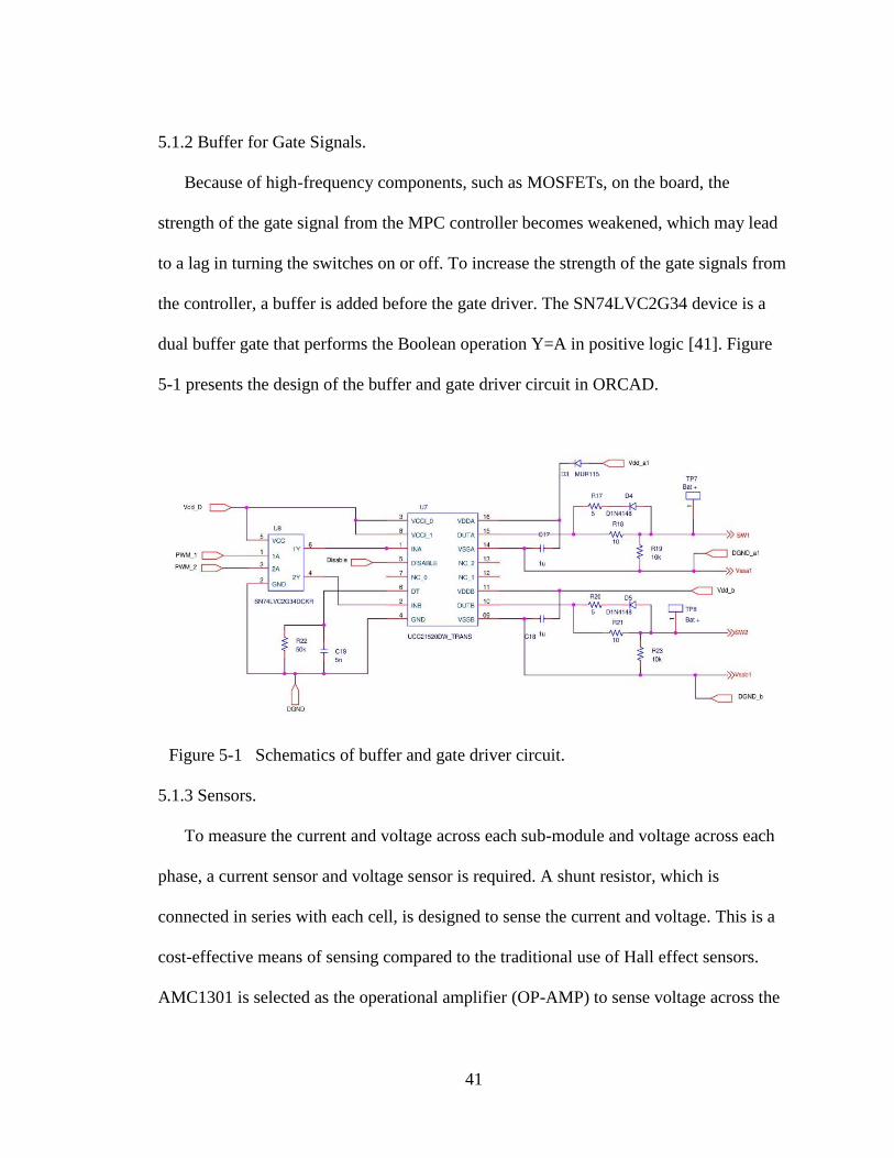
5.1.2 Buffer for Gate Signals.

Because of high-frequency components, such as MOSFETs, on the board, the

strength of the gate signal from the MPC controller becomes weakened, which may lead

to a lag in turning the switches on or off. To increase the strength of the gate signals from

the controller, a buffer is added before the gate driver. The SN74LVC2G34 device is a

dual buffer gate that performs the Boolean operation Y=A in positive logic [41]. Figure

5-1 presents the design of the buffer and gate driver circuit in ORCAD.

Figure 5-1 Schematics of buffer and gate driver circuit.

5.1.3 Sensors.

To measure the current and voltage across each sub-module and voltage across each

phase, a current sensor and voltage sensor is required. A shunt resistor, which is

connected in series with each cell, is designed to sense the current and voltage. This is a

cost-effective means of sensing compared to the traditional use of Hall effect sensors.

AMC1301 is selected as the operational amplifier (OP-AMP) to sense voltage across the

42

shunt resistor. It is a precision isolation amplifier with a nominal gain of 8.2 [43]. The

input of the AMC1301 is optimized for direct connection to shunt resistors or other

low-voltage-level signal sources.

(a) Design of shunt resistor for current sensing: As discussed previously, the

peak-to-peak current that flows through the sub-modules is ±68.72A. Considering the

peak current to be 70 A, the shunt value can be calculated as

𝑅𝑠ℎ𝑢𝑛𝑡 =±250𝑚𝑉

±70𝐴= 3.57 𝑚Ω.

Here, ±250𝑚𝑉 is the input voltage range of AMC1301 OP-AMP. The output of

AMC1301 OP-AMP is a differential signal. This output must be calibrated to a

single-ended form with a range between 0V and 3.3V before sending to the controller.

According to the datasheet of AMC1301, the input range is ±250 𝑚𝑉, with a nominal

gain of 8.2, and the output range is ±2.05 𝑚𝑉. So, the peak-to-peak value of the output

voltage for AMC1301 is 4.10 V. To reduce it to 3.3 V, another OP-AMP, OPA320, is

added between the controller and AMC1301 [42]. The OPA320 gain is given by

3.24

4.10= 0.79.

(b) Resistors selection for OPA320: The differential amplifier gain is given by

𝑅𝑓

𝑅𝑖𝑛=

7.5𝑘Ω

4.7𝑘Ω+4.7𝑘Ω = 0.79 , where 𝑅𝑓 and 𝑅𝑖𝑛 are the feedback and input resistor,

respectively. Figure 5-2 illustrates the current sensor circuit.

43

Figure 5-2 Schematics of the current sensor circuit.

(c) Design of shunt resistor for voltage sensing: The voltage sensor at the output is

designed to measure the voltage of each phase. The selected IPMM has a phase-to-phase

voltage of 96 V. Thus, the maximum phase-to-neutral voltage is 48 V. By including

voltages due to line inductance, the maximum voltage that can be sensed is 60 V.

Therefore, the shunt resistor is designed at the output of each MMC.

𝑅𝑠ℎ𝑢𝑛𝑡 =±250𝑚𝑉

±60𝑉= 4.12 𝑚Ω

Other components of the voltage sensor, such as an sensing OP-AMP (AMC1301),

analog to digital converter (OPA320), feedback, and input resistor, are selected in the

same way as the current sensor (see Figure 5-3).

44

Figure 5-3 Schematics of voltage sensor.

5.1.4 Protection Circuits.

The MMC module involves an H-bridge circuit that has a risk of shoot-through if two

switches in the same leg turn on at the same time. In a shoot-through condition, a large

amount of current flows through the MOSFETs, which can damage them. To protect the

circuit from a shoot-through condition, a protection circuit that uses TLC372 is designed

in accordance with Figure 5-4. This TLC372 consists of two independent voltage

comparators [44], each of which is designed to operate from a single power supply (3 V

to 16 V range). The voltage across the voltage divider circuit is compared with the signals

from OPA320. The diode LED is designed to light up during the overload condition. The

outputs are open-drain configurations and can be connected to achieve positive-logic

wired-AND relationships.

45

Figure 5-4 Schematics of overload protection circuit.

Besides the aforementioned components, others include the connectors to link

different sub-modules and battery cells, test points to test the voltage, and current sensor

outputs. The designed board contains four layers to increase the spacing between high

switching-frequency components, such as MOSFETs and printed circuit board (PCB)

traces.

46

CHAPTER 6. CONCLUSION AND FUTURE WORK

6.1 Conclusion

This thesis has proposed a one-step-horizon MPC scheme for a three-phase IPMM

that is fed by MMC modules. The main findings of this work are presented as follows

with their corresponding conclusions:

1) Simulation results in chapter 5 show that the tracking performance of MPC is directly

dependent on the sampling frequency of the controller. Faster controller sampling

frequency leads to better reference tracking and vice-versa. However, for performing

calculation-intensive MPC optimizations in small sample time, powerful DSPs are

needed. A larger number of sub-modules are included in MMC to overcome this

challenge. The reference tracking error decreases with the increase in number of

sub-modules. Thus, to compensate for the low sampling frequency of the DSP, the

number of sub-modules is increased in the MMC.

2) To attain the required harmonic content in the output current, the MMC with a lower

number of sub-modules switches at higher voltage and frequency compared to the

MMC with a higher number of sub-modules. Reduction in harmonics is due to the

availability of more voltage levels in the latter. Because of switching at a higher

voltage and a higher frequency, the MMC with a lower number of sub-modules have

greater switching losses.

3) The implemented cost function in MPC is adaptive and changes according to the

current tracking error. It can reduce the phase voltage ripple, relieve the

microcontroller of extra calculation burden, decrease the switching frequency, and

47

ensure the motor work under safe current limits by including the system constraints.

The current tracking performance is further improved by fine-tuning the weights of

the constraints.

4) Simulation results demonstrate that the proposed control scheme can track the

reference speed by operating in MTPA, FW and MTPV regions for maximum

efficiency.

5) The modular nature of MMC allows the control of individual battery cells in each

sub-module. An algorithm is designed to ensure that the terminal voltage levels of all

battery cells in the MMC system are equalized within the driving cycle.

6.2 Future Work

Due to time constraints, other adaptations, tests, and experiments must be left to

further investigations. This future research should concern a deeper analysis of particular

mechanisms and new methods regarding the following ideas.

1. Adding ultracapacitors to provide instantaneous power: Li-Ion cells have high

energy density but lower power density compared to ultracapacitors. During the starting

of the motor, high starting torque demands high initial current, which imposes intense

stress on battery cells. Conventional ultracapacitors have the advantage of delivering fast

bursts of power and can be recharged thousands of times without losing much capacity.

2. Include regenerative braking to recover the energy: In this thesis, an EV can use

regenerative braking to recoup energy during braking, which is not possible for

conventional ICE vehicles. Regenerative braking is the process of feeding energy from

the drive motor back into the battery during the braking process, when the vehicle’s

48

inertia forces the motor into generator mode. With the H-bridge topology of the proposed

MMC converter, the direction of the flow of current can be controlled, and regenerative

braking and charging of battery cells can hence be achieved in the proposed control

structure.

3. Increasing the horizon of MPC: The mechanical systems have a significantly low

time constant compared to electrical systems; thus it is possible to predict the future states

of the motor for a larger prediction horizon. The present thesis focuses on MPC with a

unit step horizon. However, increasing the prediction horizon should further enhance the

reference tracking performance.

4. Prediction of weights by machine learning: In the proposed control scheme, the

weights of the cost function are determined by the hit-and-trial method. However, a

machine-learning technique can predict the weights based on the state of the motor

operation. Such accurate variation of weights is expected to boost the tracking

performance of the motor.

While all of the aforementioned points will improve the performance of the systems,

addition of an ultracapacitor would improve the system’s performance many folds.

Combining the high-power density of ultracapacitor with the high energy density of

batteries can improve the performance of the EV motor, as the ultracapacitor can provide

high starting torques, and batteries can take over during steady-state operation. This

approach would decrease the high stress on battery cells due to a sudden rise in current

and would thus improve the battery life.

49

Preliminary work on the design of MMC submodule has already begun: Figure 6-1

offers the topology for this work. The cost function for the topology in this figure

would include capacitor charge and power required by the load besides the error and

constraint terms as discussed in this thesis.

Figure 6-1 Schematics of new sub-module topology.

50

REFERENCES

[1] “How Clean is Your Electric Vehicle?,” Union of Concerned Scientists. [Online].

Available: https://www.ucsusa.org/clean-vehicles/electric-vehicles/ev-emissions-

tool. [Accessed: 27-Oct-2018].

[2] K. Palmer, J. E. Tate, Z. Wadud, and J. Nellthorp, “Total cost of ownership and

market share for hybrid and electric vehicles in the UK, US and Japan,” Appl. Energy,

vol. 209, pp. 108–119, Jan. 2018.

[3] G. X. ETFs, “The Future Of Transportation Is Autonomous And Electric,” Seeking

Alpha, 17-Apr-2018. [Online]. Available: https://seekingalpha.com/article/4163546-

future-transportation-autonomous-electric. [Accessed: 27-Oct-2018]

[4] “Electrifying insights: How automakers can drive electrified vehicle sales and

profitability McKinsey.” Internet: https://www.mckinsey.com/industries/automotive-

and-assembly/our-insights/electrifying-insights-how-automakers-can-drive-

electrified-vehicle-sales-and-profitability. [Accessed: 27-Oct-2018].

[5] A. Bălţăţanu and M. Florea, “Comparison of electric motors used for electric vehicles

propulsion,” International Conference of Scientific Paper, Afases 2013, Brasov, 23-

25 May 2013.

[6] W. L. Soong and N. Ertugrul, "Field-weakening performance of interior permanent-

magnet motors," in IEEE Transactions on Industry Applications, vol. 38, no. 5, pp.

1251-1258, Sept.-Oct. 2002

[7] I. Takahashi and T. Noguchi, “A New Quick-Response and High-Efficiency Control

Strategy of an Induction Motor,” IEEE Trans. Ind. Appl., vol. IA-22, no. 5, pp. 820–

827, Sep. 1986.

[8] W. Jun, P. Hong, and J. Yu, “A simple direct-torque fuzzy control of permanent

magnet synchronous motor driver,” in Intelligent Control and Automation, 2004.

WCICA 2004. Fifth World Congress on, 2004, vol. 5, pp. 4554–4557.

[9] K. M. Tsang and W. L. Chan, “Adaptive control of power factor correction converter

using nonlinear system identification,” IEE Proc.-Electr. Power Appl., vol. 152, no.

3, pp. 627–633, 2005.

[10] J. Holtz, “A predictive controller for the stator current vector of ac machines fed from

a switched voltage source,” Proc IEE Jpn. IPEC-Tokyo83, pp. 1665–1675, 1983.

[11] P. Cortés, M. P. Kazmierkowski, R. Kennel, D. E. Quevedo, and J. R. Rodriguez,

“Predictive Control in Power Electronics and Drives.,” IEEE Trans Ind. Electron.,

vol. 55, no. 12, pp. 4312–4324, 2008.

51

[12] M. H. Moradi, “Predictive control with constraints, J.M. Maciejowski; Pearson

Education Limited, Prentice Hall, London, 2002, pp. IX+331, price £35.99, ISBN 0-

201-39823-0,” Int. J. Adapt. Control Signal Process., vol. 17, no. 3, pp. 261–262,

Apr. 2003.

[13] S. Bolognani, S. Bolognani, L. Peretti, and M. Zigliotto, “Design and

Implementation of Model Predictive Control for Electrical Motor Drives,” IEEE

Trans. Ind. Electron., vol. 56, no. 6, pp. 1925–1936, Jun. 2009.

[14] “Long-range predictive control of current regulated PWM for induction motor

drives using the synchronous reference frame - IEEE Journals & Magazine.”

[Online]. Available: https://xploresit.ieee.org/document/553670. [Accessed: 22-Oct-

2018].

[15] E. S. de Santana, E. Bim, and W. C. do Amaral, “A Predictive Algorithm for

Controlling Speed and Rotor Flux of Induction Motor,” IEEE Trans. Ind. Electron.,

vol. 55, no. 12, pp. 4398–4407, Dec. 2008.

[16] A. Linder and R. Kennel, “Model Predictive Control for Electrical Drives,” 2005,

vol. 2005, pp. 1793–1799.

[17] M. Preindl and S. Bolognani, “Model Predictive Direct Torque Control With Finite

Control Set for PMSM Drive Systems, Part 1: Maximum Torque Per Ampere

Operation,” IEEE Trans. Ind. Inform., vol. 9, no. 4, pp. 1912–1921, Nov. 2013.

[18] M. Preindl and S. Bolognani, “Model Predictive Direct Torque Control With Finite

Control Set for PMSM Drive Systems, Part 2: Field Weakening Operation,” IEEE

Trans. Ind. Inform., vol. 9, no. 2, pp. 648–657, May 2013.

[19] J. Rodriguez, Jih-Sheng Lai, and Fang Zheng Peng, “Multilevel inverters: a survey

of topologies, controls, and applications,” IEEE Trans. Ind. Electron., vol. 49, no. 4,

pp. 724–738, Aug. 2002.

[20] M. Malinowski, “Cascaded multilevel converters in recent research and

applications,” Bull. Pol. Acad. Sci. Tech. Sci., vol. Vol. 65, no. nr 5, 2017.

[21] P. V. Kapoor and M. M. Renge, “Improved Performance of Modular Multilevel

Converter for Induction Motor Drive,” Energy Procedia, vol. 117, pp. 361–368,

Jun. 2017.

[22] K. Sharifabadi, L. Harnefors, H.-P. Nee, S. Norrga, and R. Teodorescu, Design,

Control, and Application of Modular Multilevel Converters for HVDC Transmission

Systems. John Wiley & Sons, 2016.

52

[23] V. Najmi, “Modeling, Control and Design Considerations for Modular Multilevel

Converters,” Masters of science thesis, Virginia Polytechnic Institute and State

University, USA, 2015.

[24] “A New Configuration of Multilevel Inverter with Lower Number of Circuit

Elements,” ResearchGate. Internet:

https://www.researchgate.net/publication/321443827_A_New_Configuration_of_M

ultilevel_Inverter_with_Lower_Number_of_Circuit_Elements. [Accessed: 22-Oct-

2018].

[25] J. M. Kharade and D. N. G. Savagave, “A Review of HVDC Converter

Topologies,” International Journal of Innovative Research in Science, Engineering

and Technology, vol. 6, no. 2, p. 9, 2007.

[26] J. B. Rawlings and D. Q. Mayne, “Postface to ‘Model Predictive Control: Theory

and Design,’” p. 726.

[27] S. M. Goetz, A. V. Peterchev, and T. Weyh, “Modular Multilevel Converter With

Series and Parallel Module Connectivity: Topology and Control,” IEEE Trans.

Power Electron., vol. 30, no. 1, pp. 203–215, Jan. 2015.

[28] J. Kim, J. Shin, C. Chun, and B. H. Cho, “Stable Configuration of a Li-Ion Series

Battery Pack Based on a Screening Process for Improved Voltage/SOC Balancing,”

IEEE Trans. Power Electron., vol. 27, pp. 411–424.

[29] M. Kokila, P. Manimekalai, and V. Indragandhi, “Design and development of

battery management system (BMS) using hybrid multilevel converter,” Int. J.

Ambient Energy, vol. 0, no. 0, pp. 1–9, Jun. 2018

[30] Zheng, Z., Wang, K., Xu, L., & Li, Y. (2014). A hybrid cascaded multilevel converter

for battery energy management applied in electric vehicles. IEEE Transactions on

power electronics, 29(7), 3537-3546.

[31] C. French and P. Acarnley, “Direct torque control of permanent magnet drives,”

IEEE Transactions on Industry Applications, vol. 32, no. 5, pp. 1080–1088,

September/October 1996

[32] M. O. Badawy, et. al., “Integrated Control of an IPM Motor Drive and a Novel

Hybrid Energy Storage System for Electric Vehicles”, in IEEE Trans. Ind. Appl.,

2017, vol. 53, pp. 5810-5819.

53

[33] Xuecong Xu, et. al., “Predictive speed control of interior permanent magnet

synchronous motor with maximum torque per ampere control strategy,” in 36th

Chinese Control Conference, Dalian, China, Jul. 2017

[34] Leopold Sepulchre, et. al., ”New High Speed PMSM Flux-Weakening Strategy”,

19th International Conference on Electrical Machines and Systems, Chiba, Japan,

Nov. 13-16, 2016

[35] Pavel Vaclavek and Petr Blaha “Interior Permanent Magnet Synchronous Machine

High Speed Operation using Field Weakening Control Strategy”, 12th WSEAS

Conference on SYSTEMS, Heraklion, Greece, July 22-24 2008

[36] R. N. Fard, “Finite Control Set Model Predictive Control in Power Converters,”

p. 87.

[37] E. J. Fuentes, J. Rodriguez, C. Silva, S. Diaz and D. E. Quevedo, "Speed control of

a permanent magnet synchronous motor using predictive current control," 2009

IEEE 6th International Power Electronics and Motion Control Conference, Wuhan,

2009, pp. 390-395.

[38] Y. Xiong, S. Sun, H. Jia, P. Shea and Z. John Shen, "New Physical Insights on

Power MOSFET Switching Losses," in IEEE Transactions on Power Electronics,

vol. 24, no. 2, pp. 525-531, Feb. 2009

[39] Texas Instruments, “25-V N-Channel NexFET Power MOSFET,” CSD16411Q3

datasheet, August 2009 [Revised Nov. 2016].

[40] Texas Instruments, “A 4-A, 6-A, 5.7-kVRMS Isolated Dual-Channel Gate Driver,”

UCC21520, UCC21520A datasheet, June 2016 [Revised Dec. 2017].

[41] Texas Instruments, “Dual Buffer Gate,” SN74LVC2G34 datasheet, August 2001

[Revised Oct. 2015].

[42] Texas Instruments, “OPAx320x Precision, 20-MHz, 0.9-pA, Low-Noise, RRIO,

CMOS Operational Amplifier with Shutdown,” OPA320 datasheet, August 2010

[Revised Dec. 2016].

[43] Texas Instruments, “AMC1301 Precision, ±250-mV Input, 3-µs Delay, Reinforced

Isolated Amplifier,” AMC1301 datasheet, April 2016 [Revised March 2018].

[44] Texas Instruments, “LinCMOS dual differential comparators,” TLC372 datasheet,

Nov. 1983 [Revised July 2008].