ARTICLE IN PRESS

0098-3004/$ - se

doi:10.1016/j.ca

$Code on

htm.�Correspond

Fairway Drive

Zealand. Tel.: +

E-mail addr

Computers & Geosciences 34 (2008) 503–514

www.elsevier.com/locate/cageo

Application of DInSAR-GPS optimization for derivation ofthree-dimensional surface motion of the southern California

region along the San Andreas fault$

S.V. Samsonova,�, K.F. Tiampoa, J.B. Rundleb

aDepartment of Earth Sciences, University of Western Ontario, London, Ont., CanadabCenter for Computational Science and Engineering, University of California, Davis, CA, USA

Received 13 November 2006; received in revised form 27 April 2007; accepted 8 May 2007

Abstract

We present here a methodology that allows the combination of GPS and Differential InSAR data for the calculation of

continuous three-dimensional (3D) high-resolution velocity maps with corresponding errors. It is based on analytic

minimization of the Gibbs energy function, which is possible in the case when neighborhood pixels of the velocity maps are

considered independent. By joining scalar DInSAR data and vector GPS data, the technique allows us to achieve

significant improvement in accuracy in the components of the velocity vector in comparison with the GPS data alone. In

the accompanying example, the method is used for the investigation of the creep motion of the southern San Andreas fault

around the Salton Sea region. The velocity maps are calculated for two time periods (1992–1998 and 1997–2001) and also

for 3D and 2D cases. The preliminary analysis of the optimized data suggests that creep on the San Andreas fault in this

region is time-dependent.

r 2007 Elsevier Ltd. All rights reserved.

Keywords: GPS; InSAR; San Andreas fault creep

1. Introduction

In this work we present a method of merging thedata from continuous global positioning system(GPS) (Hofmann-Wellenhof et al., 2001) anddifferential interferometric synthetic aperture radar(DInSAR) (Massonnet and Feigl, 1998; Rosenet al., 2000) for derivation of high-resolution

e front matter r 2007 Elsevier Ltd. All rights reserved

geo.2007.05.013

server at: http://www.iamg.org/CGEditor/index.

ing author. Current address: GNS Science, 1

, Avalon, P.O. BOX 30368, Lower Hutt, New

64 4 570 4566; fax: +64 4 570 4600.

ess: s.samsonov@gns.cri.nz (S.V. Samsonov).

three-dimensional (3D) surface velocity maps withthe corresponding errors. The complementarynature of both geodetic techniques is evident andhas been extensively exploited (Ge et al., 2000, 2001;Gudmundsson et al., 2002; Samsonov and Tiampo,2006). The continuous GPS measures 3D coordi-nates of the GPS sites with high temporal but lowspatial resolution. Currently, there are only a fewGPS networks in the world, such as the JapaneseGEONET (Tsuda et al., 1998) and the SouthernCalifornia Integrated GPS Network (SCIGN)1

.

1Southern California Integrated GPS Network SCIGN, http://

www.scign.org/.

ARTICLE IN PRESSS.V. Samsonov et al. / Computers & Geosciences 34 (2008) 503–514504

(Bock et al., 1997), that have sufficiently densespatial coverage and are capable of measuring thesurface deformations with the resolution of approxi-mately 10–30 km. DInSAR, on the other hand,measures the total deformation between two acqui-sition scenes projected in the line-of-site (LOS) withhigh spatial resolution over a wide area, but lowtemporal resolution. The best temporal resolutionsuitable for long term continuous measurements of35 days was achieved by ERS-1/2 satellite missionsbetween 1992 and 2005, not considering tandempairs with temporal resolution of 1 day, which arenot suitable for long term deformation studies butare very useful for coseismic measurements.

In Samsonov and Tiampo (2006), we reconstructeda 3D synthetic velocity field from sparse GPSmeasurements and two differential interferograms(ascending and descending). It was shown that thismethod significantly improves the accuracy of thevelocity measurements derived from the GPS dataalone and also can be used to derive high-resolutioncontinuous maps of the surface velocity field.Unfortunately, for many regions only one type ofinterferogram is available. In Samsonov et al. (2007),only descending ERS-2 interferograms along with theGPS data from the SCIGN were used to derive a 3Dsurface velocity field of the southern California regionnear Los Angeles. It was shown that by using thistechnique, it is possible to differentiate betweenvarious deformation signals, such as anthropogenicsignal due to groundwater extraction or tectonic signaldue to plate motions.

The goal of this work is to present computer codethat is used to perform the DInSAR-GPS optimiza-tion along with some additional routines that are usedto prepare data for the optimization. The GenericMapping Tools (GMT) software package (Wessel andSmith, 1998) was used for visualization of theintermediate and final results. Almost all computa-tionally extensive routines are implemented in C/C++ language (ANSI/ISO/IEC standard) and arecalled from bash script.2 The computer code used inthis work was compiled and tested under Linux (RedHat, Fedora). Although this has not been testedspecifically, it is anticipated that the C/C++ code canbe easily recompiled to be used on Windows.

Finally, the DInSAR-GPS optimization techni-que is used to investigate the surface motion acrossthe southern part of the San Andreas fault near the

2Introduction to bash script, http://www.gnu.org/software/

bash/.

Salton Sea region. The work of Lyons and Sandwell(2003) suggest that the San Andreas fault in thatregion creeps with the approximately permanentvelocity of 1.2–1.8 cm/year and its motion is approxi-mately horizontal (strike-slip). In this work wecalculate the 3D velocity field for two time periods:1992–1998 and 1997–2001. From the results it isevident that both assumptions, permanent creepvelocity and the absence of the vertical motion acrossthe fault, are contradictory. We show that if oneassumes that the creep rates are approximatelyconstant over time then the motion across the faultcannot be considered strictly horizontal. On the otherhand, if we assume that the motion across the fault ishorizontal (strike-slip), then the creep rates varygreatly in the short time interval.

The accuracy of the optimization technique pro-posed in this work greatly depends on the number anddistribution of the GPS sites in the area (Samsonovand Tiampo, 2006). Since the linear regression of thetime series is used to calculate an initial 3D model ofthe surface velocities, it is also necessary to have asufficiently long time series in order to achieve goodaccuracy. In this work the data from seven GPS siteswere used to calculate the initial velocity model for the1992–1998 period and the data from 51 sites were usedfor the 1997–2001 period. These numbers seem to beinsufficient for a good estimation of the initial velocitymodel. Also, some DInSAR signal is not completelyunderstood; therefore, these results should be con-sidered only preliminary. They require more detailedinvestigation and validation by other sources of data,such as locally installed strainmeters.

2. Implementation

The theoretical aspects of DInSAR-GPS optimi-zation along with the complete set of the optimiza-tion equations are explained in Samsonov et al.(2007) (Eqs. (8)–(9) and (11)–(12)) and are givenhere in a brief form. In order to perform theoptimization, we construct an energy function of thefollowing form and search for its minimum withregard to its arguments

uðvx; vy; vzÞ ¼XN

i¼1

fCiinsðV

iLOS � Si

xvix � Si

yviy � Si

zvizÞ2

þ CixðV

ix � vi

xÞ2þ Ci

yðViy � vi

yÞ2

þ CizðV

iz � vi

zÞ2g ð1Þ

ARTICLE IN PRESSS.V. Samsonov et al. / Computers & Geosciences 34 (2008) 503–514 505

with coefficients

Ciins ¼

1

2ðsiinsÞ

2; Ci

x ¼1

2ðsixÞ

2; Ci

y ¼1

2ðsiyÞ

2,

Ciz ¼

1

2ðsizÞ2, ð2Þ

where ðSix;S

iy;S

izÞ is the unit vector pointing from

the ground to the satellite (LOS vector), V iLOS is the

DInSAR interferogram, ðV ix;V

iy;V

izÞ is the inter-

polated GPS velocity vector, s’s are the standarddeviations of the measurements and ðvi

x; viy; v

izÞ is the

optimized velocity vector.Since each term of uðvx; vy; vzÞ is nonnegative, its

global minimum is reached when each subgroupwith the same index i is also minimal and, therefore,the first derivatives qu=qvi

x , qu=qviy , qu=qvi

z areequal to zero. Thus, the solution of this problem isfound analytically.

2.1. Differential InSAR

There are a number of software packagescurrently available for differential InSAR proces-sing, such as the commercial EarthView packagedeveloped by Atlantis Scientific or the freewareROI_PAC from Caltech/Jet Propulsion Laboratoryand DORIS from Delft University of Technology.All these packages perform similar steps in orderto calculate the differential interferogram, such asimage coregistration, interferogram computation,baseline estimation and interferogram, attendingand removal of topographic phase. In this workall interferograms were processed by ROI_PACpackage (Rosen et al., 2004). Delft preciseorbits (Scharroo et al., 2000) were used to estimatethe exact position of the satellite during theacquisition, and SRTM Digital Elevation Model(DEM) data were used to remove the topographicphase.

From previous investigations, it is evident thatdifferential interferograms carry significant amountof useful data, such as surface deformations due toseismic events (Jacobs et al., 2002; Massonnet et al.,1993, 1996) and volcanic activities (Lundgren et al.,2003) and anthropogenic subsidence due to mining(Perski, 1999) or groundwater extraction (Shmidtand Burgmann, 2003). Different types of errors arealso present in the interferograms and these need tobe estimated and, if possible, corrected. The mostcommon error, which is easy to observe and correct,is the one due to inaccurate orbit estimation. This

error manifests itself as a linear gradient across theinterferogram (Massonnet and Feigl, 1998). There-fore, subtraction of the fitted plane from theinterferogram usually successfully corrects it. Oftenionospheric error is present, which also manifestsitself as a linear trend across interferogram. In thiscase the ionospheric error also can be removed bysubtraction of the fitted plane from the interfero-gram. However, in rare cases the linear trend is dueto long-wavelength deformation signal. We foundthat in order to ensure the nature of the signal, it issometimes useful to create a synthetic differentialinterferogram from interpolated GPS data and toanalyze the residual between the synthetic andthe differential interferograms in both (lat/long)directions.

The atmospheric water vapor effects are perhapsthe most challenging. It has been shown thateven small variations in air temperature, densityand humidity can significantly affect the signaland cause an LOS displacement of a few centimeters(Hanssen and Feijt, 1996). This error canmanifest itself either as a localized disturbance,which is most probably due to a large cloud, or as alarge area due to a large atmospheric front(Hanssen, 2001; Massonnet and Feigl, 1998). Thereare a few techniques available to compensateand reduce the atmospheric errors, such as GPS-MODIS correction (Li et al., 2005) as was donein Samsonov et al. (2007). An alternative methodis to create an interferometric stack as it wasdone in Lyons and Sandwell (2003) and also inthis work.

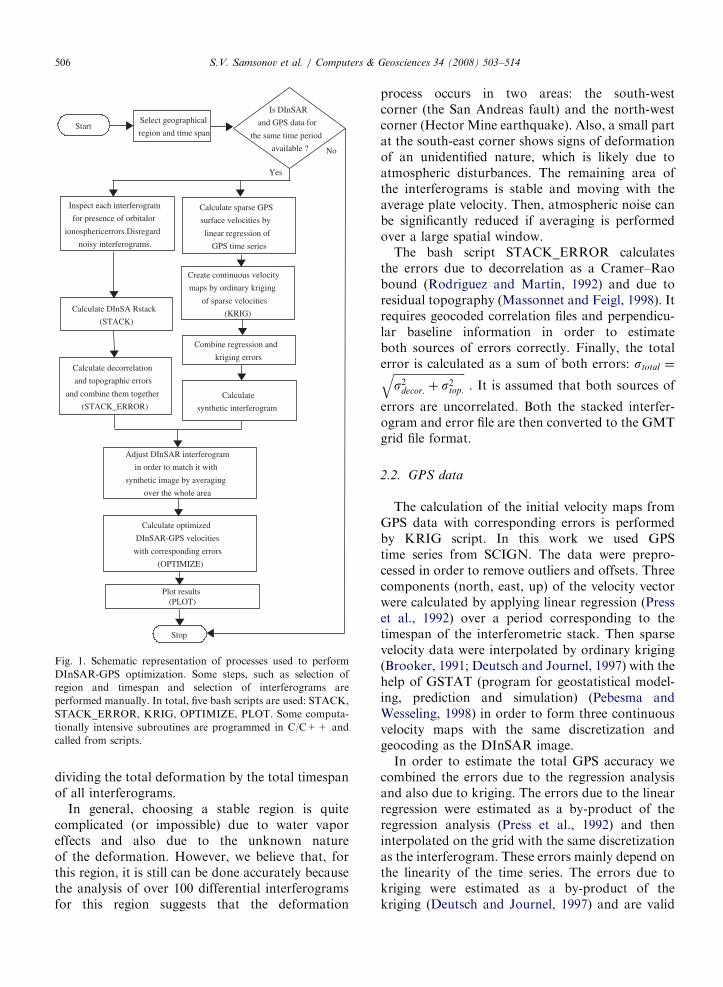
The flow chart diagram of DInSAR-GPS opti-mization is presented in Fig. 1. The bash scriptSTACK is used to calculate the interferometricstack from unwrapped interferograms. This proce-dure consist of a few steps. First the deformationvalues of each interferogram (in cm) are dividedby the timespan (in years), thereby convertingthem to velocities. Then the stable region of theinterferogram is identified and the average value forthe region is calculated. Finally, all the interfero-grams are adjusted to the same average value byadding or subtracting the difference between thereference average value and the current averagevalue, bringing all of the interferograms to acommon vertical reference frame. Then velocityvalues of the interferograms are multiplied bytimespan, thereby converting them back to displa-cements (in cm) and stack is calculated according tothe technique proposed in Wright et al. (2004)

ARTICLE IN PRESS

Start

Stop

Is DInSAR

and GPS data for

the same time period

available ?

Calculate DInSA Rstack

(STACK)

Calculate sparse GPS

surface velocities by

linear regression of

GPS time series

Create continuous velocity

maps by ordinary kriging

of sparse velocities

(KRIG)

Calculate optimized

DInSAR-GPS velocities

with corresponding errors

(OPTIMIZE)

Combine regression and

kriging errorsCalculate decorrelation

and topographic errors

and combine them together

(STACK_ERROR)

Inspect each interferogram

for presence of orbitalor

ionosphericerrors.Disregard

noisy interferograms.

Select geographical

region and time span

Plot results(PLOT)

Calculate

synthetic interferogram

Adjust DInSAR interferogram

in order to match it with

synthetic image by averaging

over the whole area

Yes

No

Fig. 1. Schematic representation of processes used to perform

DInSAR-GPS optimization. Some steps, such as selection of

region and timespan and selection of interferograms are

performed manually. In total, five bash scripts are used: STACK,

STACK_ERROR, KRIG, OPTIMIZE, PLOT. Some computa-

tionally intensive subroutines are programmed in C/C++ and

called from scripts.

S.V. Samsonov et al. / Computers & Geosciences 34 (2008) 503–514506

dividing the total deformation by the total timespanof all interferograms.

In general, choosing a stable region is quitecomplicated (or impossible) due to water vaporeffects and also due to the unknown natureof the deformation. However, we believe that, forthis region, it is still can be done accurately becausethe analysis of over 100 differential interferogramsfor this region suggests that the deformation

process occurs in two areas: the south-westcorner (the San Andreas fault) and the north-westcorner (Hector Mine earthquake). Also, a small partat the south-east corner shows signs of deformationof an unidentified nature, which is likely due toatmospheric disturbances. The remaining area ofthe interferograms is stable and moving with theaverage plate velocity. Then, atmospheric noise canbe significantly reduced if averaging is performedover a large spatial window.

The bash script STACK_ERROR calculatesthe errors due to decorrelation as a Cramer–Raobound (Rodriguez and Martin, 1992) and due toresidual topography (Massonnet and Feigl, 1998). Itrequires geocoded correlation files and perpendicu-lar baseline information in order to estimateboth sources of errors correctly. Finally, the totalerror is calculated as a sum of both errors: stotal ¼ffiffiffiffiffiffiffiffiffiffiffiffiffiffiffiffiffiffiffiffiffiffiffiffiffiffi

s2decor: þ s2top:

q. It is assumed that both sources of

errors are uncorrelated. Both the stacked interfer-ogram and error file are then converted to the GMTgrid file format.

2.2. GPS data

The calculation of the initial velocity maps fromGPS data with corresponding errors is performedby KRIG script. In this work we used GPStime series from SCIGN. The data were prepro-cessed in order to remove outliers and offsets. Threecomponents (north, east, up) of the velocity vectorwere calculated by applying linear regression (Presset al., 1992) over a period corresponding to thetimespan of the interferometric stack. Then sparsevelocity data were interpolated by ordinary kriging(Brooker, 1991; Deutsch and Journel, 1997) with thehelp of GSTAT (program for geostatistical model-ing, prediction and simulation) (Pebesma andWesseling, 1998) in order to form three continuousvelocity maps with the same discretization andgeocoding as the DInSAR image.

In order to estimate the total GPS accuracy wecombined the errors due to the regression analysisand also due to kriging. The errors due to the linearregression were estimated as a by-product of theregression analysis (Press et al., 1992) and theninterpolated on the grid with the same discretizationas the interferogram. These errors mainly depend onthe linearity of the time series. The errors due tokriging were estimated as a by-product of thekriging (Deutsch and Journel, 1997) and are valid

ARTICLE IN PRESS

Table 1

Differential interferograms used for optimization for 1992–1998

time period (left) and for 1997–2001 time period (right)

Interferogram

(1992–1998)

B ? Interferogram

(1997–2001)

B ?

930302–980424 9 970404–000428 140

950608–960802 365 980109–991210 154

951130–980109 63 980424–000602 568

990129–000915 20

S.V. Samsonov et al. / Computers & Geosciences 34 (2008) 503–514 507

for each discretization point or pixel on thecontinuous GPS velocity map. It is equal to zeroat the location of the GPS sites and increases withdistance from the known position. Therefore, itreaches a maximum at the most remote areas.Finally, both errors were combined together inorder to be used as weighting parameters for theoptimization.

2.3. Optimization and error estimation

After both DInSAR and GPS data were preparedand corresponding errors were estimated, theoptimization was performed by running the OPTI-MIZE script. This script calls a compiled C++binary program which performs the optimization.The output of the program is six binary files of theoptimized velocity model (north, east, up) withcorresponding errors (one standard deviation). Thevisualization is performed by the PLOT script,which uses GMT routines. The California faults andGPS sites that are used for the optimization are alsoplotted as black lines and black dots in order toenhance the appearance.

3. Reversal of motion across San Andreas fault

In this section the results of the DInSAR-GPSoptimization are presented. Originally over 100differential interferograms were calculated for theSalton Sea region (track 356, frame 2925) spanning

-4

-2

0

2

4

6

8

1992 1993 1994 1995 1996

LO

S v

elo

city, cm

/year

Time,

The value of the average

velocity across the

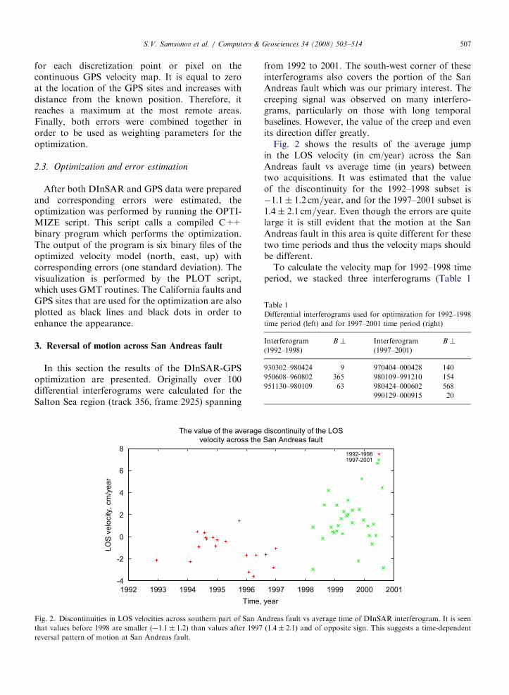
Fig. 2. Discontinuities in LOS velocities across southern part of San A

that values before 1998 are smaller ð�1:1� 1:2Þ than values after 1997

reversal pattern of motion at San Andreas fault.

from 1992 to 2001. The south-west corner of theseinterferograms also covers the portion of the SanAndreas fault which was our primary interest. Thecreeping signal was observed on many interfero-grams, particularly on those with long temporalbaselines. However, the value of the creep and evenits direction differ greatly.

Fig. 2 shows the results of the average jumpin the LOS velocity (in cm/year) across the SanAndreas fault vs average time (in years) betweentwo acquisitions. It was estimated that the valueof the discontinuity for the 1992–1998 subset is�1:1� 1:2 cm=year, and for the 1997–2001 subset is1:4� 2:1 cm=year. Even though the errors are quitelarge it is still evident that the motion at the SanAndreas fault in this area is quite different for thesetwo time periods and thus the velocity maps shouldbe different.

To calculate the velocity map for 1992–1998 timeperiod, we stacked three interferograms (Table 1

1997 1998 1999 2000 2001

year

discontinuity of the LOS

San Andreas fault

1992-19981997-2001

ndreas fault vs average time of DInSAR interferogram. It is seen

ð1:4� 2:1Þ and of opposite sign. This suggests a time-dependent

ARTICLE IN PRESS

-116°30' -115°45' -115°00' -116°30' -115°45' -115°00' -116°30' -115°45' -115°00'

-116°30' -115°45' -115°00' -116°30' -115°45' -115°00' -116°30' -115°45' -115°00'

-116°30' -115°45' -115°00' -116°30' -115°45' -115°00'

33°00'

33°15'

33°30'

33°45'

34°00'

34°15'

34°30'

0 12.525

km

-5 -4 -3 -2 -1 0 1 2

cm/year

33°00'

33°15'

33°30'

33 45'

34°00'

34°15'

34°30'

0 12.525

km

-5 -4 -3 -2 -1 0 1 2

cm/year

33°00'

33°15'

33°30'

33°45'

34°00'

34°15'

34°30'

0 12.525

km

-5 -4 -3 -2 -1 0 1 2

cm/year

33°00'

33°15'

33°30'

33°45'

34°00'

34°15'

34°30'

0 12.525

km

-5 -4 -3 -2 -1 0 1 2cm/year

33°00'

33°15'

33°30'

33°45'

34°00'

34°15'

34°30'

0 12.525

km

-5 -4 -3 -2 -1 0 1 2cm/year

33°00'

33°15'

33°30'

33°45'

34°00'

34°15'

34°30'

0 12.525

km

-5 -4 -3 -2 -1 0 1 2

cm/year

33°00'

33°15'

33°30'

33°45'

34°00'

34°15'

34°30'

0 12.5 25

km

-5 -4 -3 -2 -1 0 1 2

cm/year

33°00'

33°15'

33°30'

33°45'

34°00'

34°15'

34°30'

0 12.5 25

km

0.05 0.10 0.15 0.20

cm/year

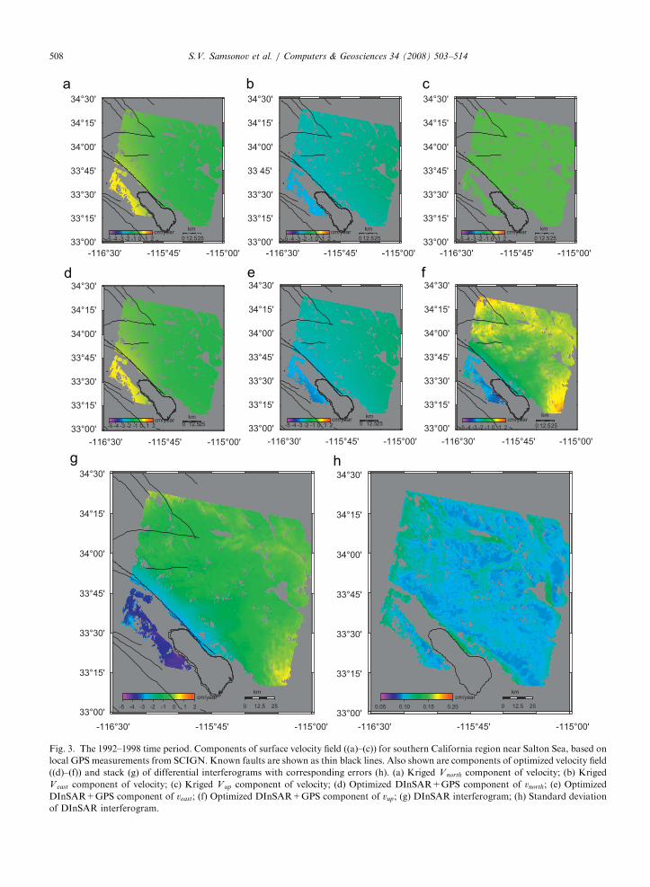
Fig. 3. The 1992–1998 time period. Components of surface velocity field ((a)–(c)) for southern California region near Salton Sea, based on

local GPS measurements from SCIGN. Known faults are shown as thin black lines. Also shown are components of optimized velocity field

((d)–(f)) and stack (g) of differential interferograms with corresponding errors (h). (a) Kriged Vnorth component of velocity; (b) Kriged

Veast component of velocity; (c) Kriged V up component of velocity; (d) Optimized DInSAR+GPS component of vnorth; (e) Optimized

DInSAR+GPS component of veast; (f) Optimized DInSAR+GPS component of vup; (g) DInSAR interferogram; (h) Standard deviation

of DInSAR interferogram.

S.V. Samsonov et al. / Computers & Geosciences 34 (2008) 503–514508

ARTICLE IN PRESS

33°00'

33°15'

33°30'

33°45'

34°00'

34°15'

34°30'

0 12.5 25

km

-5 -4 -3 -2 -1 0 1 2

cm/year

33°00'

33°15'

33°30'

33°45'

34°00'

34°15'

34°30'

0 12.5 25

km

-5 -4 -3 -2 -1 0 1 2

cm/year

33°00'

33°15'

33°30'

33°45'

34°00'

34°15'

34°30'

0 12.525

km

-5 -4 -3 -2 -1 0 1 2

cm/year

33°00'

33°15'

33°30'

33°45'

34°00'

34°15'

34°30'

0 12.5 25

km

-5 -4 -3 -2 -1 0 1 2

cm/year

33°00'

33°15'

33°30'

33°45'

34°00'

34°15'

34°30'

0 12.525

km

-5 -4 -3 -2 -1 0 1 2

cm/year

33°00'

33°15'

33°30'

33°45'

34°00'

34°15'

34°30'

0 12.525

km

-4 -2 0 2 4 6

cm/year

33°00'

33°15'

33°30'

33°45'

34°00'

34°15'

34°30'

0 12.5 25

km

-4 -2 0 2 4 6

cm/year

33°00'

33°15'

33°30'

33°45'

34°00'

34°15'

34°30'

0 12.5 25

km

0.05 0.10 0.15 0.20

cm/year

-116°30' -115°45' -115°00' -116°30' -115°45' -115°00' -116°30' -115°45' -115°00'

-116°30' -115°45' -115°00'

-116°30' -115°45' -115°00' -116°30' -115°45' -115°00'

-116°30' -115°45' -115°00' -116°30' -115°45' -115°00'

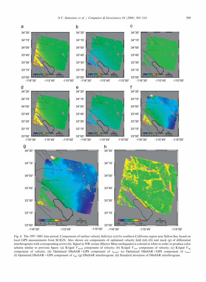
Fig. 4. The 1997–2001 time period. Components of surface velocity field ((a)–(c)) for southern California region near Salton Sea, based on

local GPS measurements from SCIGN. Also shown are components of optimized velocity field ((d)–(f)) and stack (g) of differential

interferograms with corresponding errors (h). Signal in NW corner (Hector Mine earthquake) is colored in white in order to produce color

scheme similar to previous figure. (a) Kriged Vnorth component of velocity; (b) Kriged Veast component of velocity; (c) Kriged Vup

component of velocity; (d) Optimized DInSAR+GPS component of vnorth; (e) Optimized DInSAR+GPS component of veast;

(f) Optimized DInSAR+GPS component of vup; (g) DInSAR interferogram; (h) Standard deviation of DInSAR interferogram.

S.V. Samsonov et al. / Computers & Geosciences 34 (2008) 503–514 509

ARTICLE IN PRESSS.V. Samsonov et al. / Computers & Geosciences 34 (2008) 503–514510

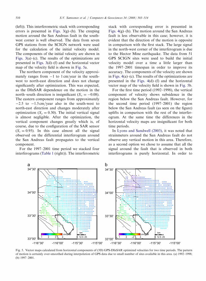
(left)). This interferometric stack with correspondingerrors is presented in Figs. 3(g)–(h). The creepingmotion around the San Andreas fault in the south-west corner is well observed. The data from sevenGPS stations from the SCIGN network were usedfor the calculation of the initial velocity model.The components of the initial velocity are shown inFigs. 3(a)–(c). The results of the optimizations arepresented in Figs. 3(d)–(f) and the horizontal vectormap of the velocity field is shown in Fig. 5a.

The northern component of the velocity approxi-mately ranges from �1 to 1 cm/year in the south-west to north-east direction and does not changesignificantly after optimization. This was expected,as the DInSAR dependence on the motion in thenorth–south direction is insignificant ðSx ¼ �0:08Þ.The eastern component ranges from approximately�2:5 to �1:5 cm=year also in the south-west tonorth-east direction and changes moderately afteroptimization ðSy ¼ 0:30Þ. The initial vertical signalis almost negligible. After the optimization, thevertical component changes greatly which is, ofcourse, due to the configuration of the SAR sensorðSz ¼ 0:95Þ. In this case almost all the signalobserved on the differential interferogram aroundthe San Andreas fault propagates to the verticalcomponent.

For the 1997–2001 time period we stacked fourinterferograms (Table 1 (right)). The interferometric

-116°30' -116°00' -115°30' -115°00'

33°00'

33°30'

34°00'

34°30'

0 12.5 25

km

1 2 3 4

cm/year

33

33

34

34

Fig. 5. Vector maps calculated from horizontal components of (3D) GP

of motion is certainly over-smoothed during interpolation of GPS data

(b) 1997–2001.

stack with corresponding error is presented inFigs. 4(g)–(h). The motion around the San Andreasfault is less observable in this case; however, it isevident that the direction of the motion is oppositein comparison with the first stack. The large signalin the north-west corner of the interferogram is dueto the Hector Mine earthquake. The data from 51GPS SCIGN sites were used to build the initialvelocity model over a time a little larger thanthe 1997–2001 timespan in order to improve itsaccuracy. The components of the velocity are shownin Figs. 4(a)–(c). The results of the optimizations arepresented in the Figs. 4(d)–(f) and the horizontalvector map of the velocity field is shown in Fig. 5b.

For the first time period (1992–1998), the verticalcomponent of velocity shows subsidence in theregion below the San Andreas fault. However, forthe second time period (1997–2001) the regionbelow the San Andreas fault (as seen on the figure)uplifts in comparison with the rest of the interfer-ogram. At the same time the differences in thehorizontal velocity maps are insignificant for bothtime periods.

In Lyons and Sandwell (2003), it was noted thatstrainmeters around the San Andreas fault do notobserve any vertical motion in this area. Therefore,as a second option we chose to assume that all thesignal around the fault that is observed in bothinterferograms is purely horizontal. In order to

-116°30' -116°00' -115°30' -115°00'

°00'

°30'

°00'

°30'

0 12.5 25

km

1 2 3 4

cm/year

S-DInSAR optimized velocities for two time periods. The pattern

due to small number of sites available in this area. (a) 1992–1998;

ARTICLE IN PRESSS.V. Samsonov et al. / Computers & Geosciences 34 (2008) 503–514 511

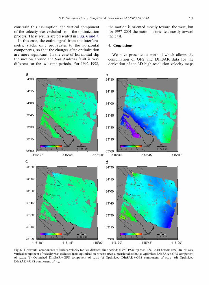
constrain this assumption, the vertical componentof the velocity was excluded from the optimizationprocess. These results are presented in Figs. 6 and 7.

In this case, the entire signal from the interfero-metric stacks only propagates to the horizontalcomponents, so that the changes after optimizationare more significant. In the case of horizontal slipthe motion around the San Andreas fault is verydifferent for the two time periods. For 1992–1998,

33°00'

33°15'

33°30'

33°45'

34°00'

34°15'

34°30'

0 12.5 25

km

-10 -5 0 5 10

cm/year

3

3

3

3

3

3

3

33°00'

33°15'

33°30'

33°45'

34°00'

34°15'

34°30'

0 12.5 25

km

-10 -5 0 5 10

cm/year

3

3

3

3

3

3

3

-116°30' -115°45' -115°00'

-116°30' -115°45' -115°00'

Fig. 6. Horizontal components of surface velocity for two different time

vertical component of velocity was excluded from optimization process (

of vnorth; (b) Optimized DInSAR+GPS component of veast; (c) O

DInSAR+GPS component of veast.

the motion is oriented mostly toward the west, butfor 1997–2001 the motion is oriented mostly towardthe east.

4. Conclusions

We have presented a method which allows thecombination of GPS and DInSAR data for thederivation of the 3D high-resolution velocity maps

3°00'

3°15'

3°30'

3°45'

4°00'

4°15'

4°30'

0 12.5 25

km

-10 -5 0 5 10

cm/year

3°00'

3°15'

3°30'

3°45'

4°00'

4°15'

4°30'

0 12.5 25

km

-10 -5 0 5 10

cm/year

-116°30' -115°45' -115°00'

-116°30' -115°45' -115°00'

periods (1992–1998 top row, 1997–2001 bottom row). In this case

two-dimensional case). (a) Optimized DInSAR+GPS component

ptimized DInSAR+GPS component of vnorth; (d) Optimized

ARTICLE IN PRESS

-116°30' -116°00' -115°30' -115°00'

33°00'

33°30'

34°00'

34°30'

0 12.5 25

km

0 2 4 6 8 10

cm/year

-116°30' -116°00' -115°30' -115°00'

33°00'

33°30'

34°00'

34°30'

0 12.5 25

km

0 2 4 6 8 10

cm/year

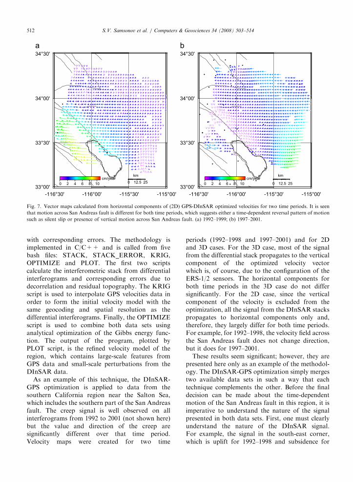
Fig. 7. Vector maps calculated from horizontal components of (2D) GPS-DInSAR optimized velocities for two time periods. It is seen

that motion across San Andreas fault is different for both time periods, which suggests either a time-dependent reversal pattern of motion

such as silent slip or presence of vertical motion across San Andreas fault. (a) 1992–1999; (b) 1997–2001.

S.V. Samsonov et al. / Computers & Geosciences 34 (2008) 503–514512

with corresponding errors. The methodology isimplemented in C/C++ and is called from fivebash files: STACK, STACK_ERROR, KRIG,OPTIMIZE and PLOT. The first two scriptscalculate the interferometric stack from differentialinterferograms and corresponding errors due todecorrelation and residual topography. The KRIGscript is used to interpolate GPS velocities data inorder to form the initial velocity model with thesame geocoding and spatial resolution as thedifferential interferograms. Finally, the OPTIMIZEscript is used to combine both data sets usinganalytical optimization of the Gibbs energy func-tion. The output of the program, plotted byPLOT script, is the refined velocity model of theregion, which contains large-scale features fromGPS data and small-scale perturbations from theDInSAR data.

As an example of this technique, the DInSAR-GPS optimization is applied to data from thesouthern California region near the Salton Sea,which includes the southern part of the San Andreasfault. The creep signal is well observed on allinterferograms from 1992 to 2001 (not shown here)but the value and direction of the creep aresignificantly different over that time period.Velocity maps were created for two time

periods (1992–1998 and 1997–2001) and for 2Dand 3D cases. For the 3D case, most of the signalfrom the differential stack propagates to the verticalcomponent of the optimized velocity vectorwhich is, of course, due to the configuration of theERS-1/2 sensors. The horizontal components forboth time periods in the 3D case do not differsignificantly. For the 2D case, since the verticalcomponent of the velocity is excluded from theoptimization, all the signal from the DInSAR stackspropagates to horizontal components only and,therefore, they largely differ for both time periods.For example, for 1992–1998, the velocity field acrossthe San Andreas fault does not change direction,but it does for 1997–2001.

These results seem significant; however, they arepresented here only as an example of the methodol-ogy. The DInSAR-GPS optimization simply mergestwo available data sets in such a way that eachtechnique complements the other. Before the finaldecision can be made about the time-dependentmotion of the San Andreas fault in this region, it isimperative to understand the nature of the signalpresented in both data sets. First, one must clearlyunderstand the nature of the DInSAR signal.For example, the signal in the south-east corner,which is uplift for 1992–1998 and subsidence for

ARTICLE IN PRESSS.V. Samsonov et al. / Computers & Geosciences 34 (2008) 503–514 513

1997–2001, is not easily explained. Also, it is notclear if the signal around the San Andreas faultdirectly corresponds to deformation signal. Part ofthis signal might be due to changes in the physicalproperties of the material around the fault such asdensity, temperature or water content.

Second, it is evident from our previous workthat seven (as in the first time period) and 51 (as inthe second time period) GPS stations are notenough to create a good initial model. We believethat the initial velocity model which is used inthis work is oversimplified and does not captureexactly the velocity pattern around and across thefault. Therefore, more GPS stations need to beinstalled and operated for a long time before asatisfactory initial velocity model of the region canbe constructed.

Despite the practical difficulties in the realizationof this method, it can be used for the investigationof surface motion in many regions of the world andargues for the increased procurement and avail-ability of these high-quality geodetic data sets.

Acknowledgments

This work was funded by an NSERC Discoverygrant and also by CSEG, KEGS Pioneers and SEGscholarships received by S. Samsonov. The work ofK. Tiampo was supported by an NSERC DiscoveryGrant. Research by J. Rundle has been supportedby a grant from the US National Aeronautics andSpace Administration under grant NAG5-13743 tothe University of California, Davis. Technicalsupport for this work has been provided by thePOLARIS network. The ERS data were obtainedfrom the WINSAR Consortium and processedby the Repeat Orbit Interferometry Package(ROI_PAC) developed at Caltech/Jet PropulsionLaboratory. The SRTM DEM data were providedby USGS and the ERS precise orbits were providedby Delft University of Technology. The GPS datawere downloaded from the SCIGN web site (http://www.scign.org) and interpolated using the GSTATpackage. The images were plotted with the help ofGMT software developed and supported by PaulWessel and Walter H.F. Smith.

References

Bock, Y., Wdowinski, S., Fang, P., Zhang, J., Behr, J.,

Genrich, J., Williams, S., Agnew, D., Wyatt, F., Johnson,

H., Stark, K., Oral, B., Hudnut, K., Dinardo, S., Young, W.,

Jackson, D., Gurtner, W., 1997. Southern California

permanent GPS geodetic array: continuous measurements of

crustal deformation between the 1992 Landers and 1994

Northridge earthquakes. Journal of Geophysical Research

108, 18013–18033.

Brooker, P., 1991. A Geostatistical Primer. World Scientific,

Singapore, 95pp.

Deutsch, C., Journel, A., 1997. GSLIB Geostatistical Software

Library and User’s Guide, second ed. Oxford University

Press, New York, 384pp.

Ge, L., Han, S., Rizos, C., 2000. Interpolation of GPS results

incorporating geophysical and InSAR information. Earth,

Planets and Space 52 (11), 999–1002.

Ge, L., Rizors, C., Han, S., Zebker, H., 2001. Mine subsidence

monitoring using the combined InSAR and GPS approach.

Technical Report, 10th FIG International Symposium on

Deformation Measurements, Orange, California, 10pp.

Gudmundsson, S., Sigmundsson, F., Carstensen, J., 2002.

Three-dimensional surface motion maps estimated from

combined interferometric synthetic aperture radar and

GPS data. Journal of Geophysical Research 107 (B10),

2250–2264.

Hanssen, R., 2001. Radar Interferometry: Data Interpretation

and Error Analysis, First ed. Kluwer Academic Publishers,

Dordrecht, 328pp.

Hanssen, R., Feijt, A., 1996. A first quantative evaluation of

atmospheric effects on SAR interferometry. In: Proceedings

of the Fringe 96 Workshop, Zurich, Switzerland.

Hofmann-Wellenhof, B., Lichtenegger, H., Collins, J., 2001. GPS

Theory and Practice. Springer, Berlin.

Jacobs, A., Sandwell, D., Fialko, Y., Sichoix, L., 2002. The

1997 (M 7.1) Hector Mine, California, earthquake:

Near-field postseismic deformation from ERS interferometry.

BSSA Special Issue on Hector Mine Earthquake 92 (4),

1433–1442.

Li, Z., Muller, J.-P., Cross, P., Fielding, E.J., 2005. Interfero-

metric synthetic aperture radar (InSAR) atmospheric correc-

tion: GPS, Moderate Resolution Imaging Spectroradiometer

(MODIS), and InSAR integration. Journal of Geophysical

Research 110 (B03410).

Lundgren, P., Berardino, P., Coltelli, M., Fornaro, G., Lanari,

R., Puglisi, G., Sansosti, E., Tesauro, M., 2003. Coupled

magma chamber inflation and sector collapse slip observed

with synthetic aperture radar interferometry on Mt. Etna

volcano. Journal of Geophysical Research 108 (B5),

2247–2262.

Lyons, S., Sandwell, D., 2003. Fault creep along the southern San

Andreas from interferometric synthetic aperture radar,

permanent scatterers and stacking. Journal of Geophysical

Research 108 (B1, 2047).

Massonnet, D., Feigl, K., 1998. Radar interferometry and its

application to changes in the Earth surface. Reviews of

Geophysics 36 (4), 441–500.

Massonnet, D., Feigl, K., Vadon, H., Rossi, M., 1996. Coseismic

deformation field of the M ¼ 6:7 Northridge, California

earthquake of January 17, 1994, recorded by two radar

satellites using interferometry. Geophysical Research Letters

23 (9), 969–972.

Massonnet, D., Rossi, M., Carmona, C., Adragna, F., Peltzer,

G., Feigl, K., 1993. The displacement field of the Landers

earthquake mapped by radar interferometry. Nature 364,

138–142.

ARTICLE IN PRESSS.V. Samsonov et al. / Computers & Geosciences 34 (2008) 503–514514

Pebesma, E.J., Wesseling, C.G., 1998. Gstat: a program for

geostatistical modelling, prediction and simulation. Compu-

ters & Geosciences 24 (1), 17–31.

Perski, Z., 1999. ERS InSAR data for geological interpretation

of mining subsidence in Upper Silesian coal basin in

Poland. In: Proceedings of the Fringe 99 Workshop, Liege,

France.

Press, W., Teukolsky, S., Vetterling, W., Flannery, B., 1992.

Numerical Recipes in C: The Art of Scientific Computing,

second ed. Cambridge University Press, Cambridge, 994pp.

Rodriguez, E., Martin, J., 1992. Theory and design of interfero-

metric synthetic aperture radars. Proceedings of the IEEE 139

(2), 147–159.

Rosen, P., Hensley, P., Joughin, I., Li, F., Madsen, S., Rodriguez,

E., Goldstein, R., 2000. Synthetic aperture radar interfero-

metry. Proceedings of the IEEE 88 (3), 333–382.

Rosen, P., Hensley, S., Peltzer, G., Simons, M., 2004. Updated

repeat orbit interferometry package released. EOS Transac-

tions, American Geophysical Union 85 (5), 47.

Samsonov, S., Tiampo, K., 2006. Analytical optimization of

DInSAR and GPS dataset for derivation of three-dimensional

surface motion. Geoscience and remote sensing letters 3 (1),

107–111.

Samsonov, S., Tiampo, K., Rundle, J., Li, Z., 2007. Application

of DInSAR-GPS optimization for derivation of fine scale

surface motion maps of southern California. Transactions on

Geoscience and Remote Sensing 45 (2), 512–521.

Scharroo, R., Visser, P., Peacock, N., 2000. ERS orbit

determination and gravity model tailoring: recent develop-

ments. In: European Space Agency Special Publication, ESA

SP-461, p. 11.

Shmidt, D., Burgmann, R., 2003. Time-dependent land uplift and

subsidence in the Santa Clara valley, California, from a large

interferometric synthetic aperture radar data set. Journal of

Geophysical Research 108 (B9), 2416.

Tsuda, T., Heki, K., Miyazaki, S., Aonashi, K., Hirahara, K.,

Nakamura, H., Tobita, M., Kimata, F., Tabei, T., Matsush-

ima, T., Kimura, F., Satomura, M., Kato, T., Naito, I., 1998.

GPS meteorology project of Japan–exploring frontiers of

geodesy. Earth Planets and Space 50 (10), i–v.

Wessel, P., Smith, W., 1998. New, improved version of the

generic mapping tools released. EOS Transactions, American

Geophysical Union 79, 579.

Wright, T., Parsons, B., England, P., Fielding, E., 2004. InSAR

observations of low slip rates on the major faults of western

Tibet. Science 305, 236–239.