application of airborne lidar in river environments: the...

Earth Surface Processes and LandformsEarth Surf. Process. Landforms 28, 299–306 (2003)Published online in Wiley InterScience (www.interscience.wiley.com). DOI: 10.1002/esp.482

APPLICATION OF AIRBORNE LIDAR IN RIVER ENVIRONMENTS:THE RIVER COQUET, NORTHUMBERLAND, UK

M. E. CHARLTON,1* A. R. G. LARGE1 AND I. C. FULLER2

1 Department of Geography, University of Newcastle, Newcastle upon Tyne, NE1 7RU, UK2 Division of Geography, University of Northumbria, Newcastle upon Tyne, NE1 8ST, UK

Received 10 July 2001; Revised 12 July 2002; Accepted 1 August 2002

ABSTRACT

The potential offered by LiDAR (laser-induced direction and ranging) for the mapping of gravel-bed river environments isaddressed in this paper. A LiDAR dataset was obtained for a reach of the River Coquet, Northumberland, UK. Topographicdata were acquired from the field at the same time using theodolite-EDM survey of a number of cross-profiles across theactive river channel and bar units. These cross-profiles provide a means of comparing measurements from the LiDARdata with ground survey. Ordnance Survey large-scale mapping was used to georeference the survey data, which werethen integrated with the LiDAR dataset using GIS software. A close correspondence between ground survey-derivedcross-profiles and those generated using LiDAR is observed. However, the presence of both vegetation and deep waterintroduces anomalies in the LiDAR surface. Correction for these anomalies is needed to improve the accuracy of LiDARmapping in the UK context and similar river environments. It is concluded that LiDAR has potential as an accuratesurvey tool for obtaining high resolution topographic data from unvegetated, exposed bar surfaces. Copyright 2003John Wiley & Sons, Ltd.

KEY WORDS: LiDAR; river channel; cross-profile; surface quality

INTRODUCTION

Intensive mapping of river channel topography in large (>1 km) dynamic reaches using traditional groundsurvey or analytical (manual) photogrammetry may exert a high demand on operator time and cost, especiallywhen including the survey of morphological detail which is at a scale larger than the gross channel-bar unit.Sub-bar morphology (e.g. chute channels, sediment lobes) may be ignored to rationalize time in the field, orat the photogrammetric plotter; however, these features may represent significant changes in sediment storagewithin the channel system (Fuller et al., 2002). Whilst digital automated photogrammetry (e.g. Westawayet al., 2000) can be used at a range of spatial scales to overcome some of these deficiencies, airborne LiDARis a potentially useful development for the acquisition of such terrain data. While differential GPS also haspotential for rapid topographic data acquisition (e.g. Brasington et al., 2000), areal extent does remain alimiting factor. LiDAR, on the other hand, permits rapid gathering of topographic data for large areas, up to90 km2 per hour (Marks and Bates, 2000).

LiDAR, variously termed in the literature as ‘laser-induced direction and ranging’ (e.g. Marks and Bates,2000) or ‘light detection and ranging’ (e.g. Optech, 2001), provides laser-based measurements of the distancebetween an aircraft carrying the sensor and the ground. The resulting measurements can be post-processedto provide a digital elevation model with a precision within 15 cm (Fowler, 2000). LiDAR consequentlyhas significant potential for generating a high-resolution digital terrain surface of complex river channelenvironments incorporating morphological features at a range of scales. Its precision when applied in gravel-bed river systems is untested, and this paper evaluates the extent to which LiDAR may be used to providereliable measurements of topography in such environments.

* Correspondence to: M. E. Charlton, Department of Geography, Daysh Building, University of Newcastle, Newcastle upon Tyne,NE1 7RU, UK. E-mail: [email protected]

Copyright 2003 John Wiley & Sons, Ltd.

300 M. E. CHARLTON, A. R. G. LARGE AND I. C. FULLER

Airborne laser techniques have been widely applied in physical geography (Innes and Koch, 1998;Bissonnette et al., 1997; McHenry et al., 1982; Parson et al., 1997; Irish and White, 1998; Gauldie et al.,1996; Krabill et al., 1995; Wadhams, 1995; Ritchie et al., 1992, 1996). Within geomorphology, the use ofairborne laser scanning has focused particularly on the measurement of ephemeral channels and gullies (e.g.Jackson et al., 1988; Ritchie and Jackson, 1989; Ritchie et al., 1994, 1995) and assessment of flood risk(Marks and Bates, 2000).

The integration of LiDAR with airborne GPS facilitates the wider use of high resolution DEMs in physicalapplications (e.g. Marks and Bates, 2000). The method of survey is rapid, relatively economic, allows surveyof difficult terrain, and large areas (for example a river catchment). This would appear to make it an attractivealternative to ground-based survey methods. However, it is difficult to determine the level of precision ofLiDAR measurements for any one survey. This feature has been identified by Brinkman and O’Neill (2000),who observe that elevations are generated from three sources: (i) the LiDAR sensor, (ii) the inertial navigationunit (INU) of the aircraft and (iii) GPS. The LiDAR measurements must be corrected for the pitch, roll andyaw of the aircraft, and the GPS information allows the slant distances to be corrected and converted into ameasurement of ground elevation relative to the WGS84 datum. The measurements are taken from side toside in a swath as the aircraft flies along its path; those measurements at the centreline of the swath are moreprecise than those near the edge. Brinkman and O’Neill (2000) also observe that both horizontal and verticalprecision depend on the flying height (where horizontal precision is 1/2000th of the flying height); horizontalprecision will thus be ‘accurate to 15 centimetres or better’ when the flying height is at or below 1200 m(Brinkman and O’Neill, 2000). In complex topography, small lateral offsets associated with the INU and GPSwill be translated into vertical error in the LiDAR surface. This is less of a problem on open, unvegetatedsurfaces than in areas with tall vegetation cover. If the flight layout can be optimized for GPS (with at leastsix satellites in view) then precisions of 7–8 cm are theoretically achievable.

The Environment Agency (EA) has commissioned LiDAR surveys of a number of river and coastal envi-ronments. The output from the flights and subsequent data processing is a series of DEMs with densities in theorder of 64 600 topographic measurements per km2 (Marks and Bates, 2000). This is equivalent to a resolutionof 3Ð9 m�1 (

p1 000 000 m2/

p64 000 measurements). Figure 1 depicts a mosaic of two adjacent 1 km2 tiles

(nt9502 and nt9602) viewed as an illuminated surface from the southwest. No vertical exaggeration has beenapplied. As well as showing the undulation of the valley sides, and some faintly visible palaeochannels onthe floodplain, vegetation cover is clearly visible. In the study area, white patches indicate where the LiDARsensor has failed to make a reading. It should be noted that these data gaps are all in the river channel.

Superimposed on Figure 1 is the outline of the area incorporating the study reach on the River Coquetat Holystone (OSGR: NY 958027), located some 25 km downstream from the river’s source in the CheviotHills and draining a subcatchment area of some 225 km2 (Figure 2). The contemporary active channel atHolystone is locally divided by expanses of bare gravel, but has well defined pool–riffle units, fitting thecriteria for a wandering channel type (Ferguson and Werritty, 1983), and displaying a complex assemblageof channel, bar and sub-bar morphology (Fuller et al., 2002). From historical maps dating back over the past150 years, the Coquet in this locality is seen to be characterized by a high degree of lateral instability andchannel avulsion. Recent calculations show volumes of sediment in excess of 2000 m3 to be reworked onan annual basis within the reach (Fuller et al., 2002). The question remains, however, as to the applicabilityof LiDAR data in the context of reach-scale topographic mapping of such gravel-bed channel systems. Inorder to address this, we compare measurements taken from the LiDAR data with spatially correspondingmeasurements obtained from tachometric survey for a series of cross-sections along the reach.

METHODS

Post-processed LiDAR data, derived from a single pulse scanning sensor, were obtained by the EA throughoutthe River Coquet catchment on 19 March 1998. No assessments of precision were available for this data set.The LiDAR measurements were georeferenced using the WGS84 datum used by the NAVSTAR GlobalPositioning System. Prior to any integration with Ordnance Survey (OS) data, all measurements had to be

Copyright 2003 John Wiley & Sons, Ltd. Earth Surf. Process. Landforms 28, 299–306 (2003)

AIRBORNE LIDAR IN RIVER ENVIRONMENTS 301

Figure 1. Perspective, viewed from the southwest, of the LiDAR elevation surface of a section of the River Coquet, showing the locationof the study reach. The area shown is 2 km ð 1 km. Flow is from northwest to southeast

North0 5 10 Km

COQUETBASIN

R.A

lwin

AMBLE

ROTHBURYHOLYSTONE

HARBOTTLE

ALWINTON

Simonside Hills

BrownshartLaw

TheCheviot

BloodybushEdge

Ch

ev

i ot H i l l s

Study reach

Feet MetresHEIGHT

2000 6101000 305400 122200 61

0 0

Gauging station

R. Coquet

R. Coquet

Forest Burn

U

sway

Bur

n

R. Coquet

Wre igh Burn

Figure 2. River Coquet catchment, Northumberland, UK, showing the location of the study reach

transformed to use the OSGB36 datum; this was carried out by the EA (Environment Agency, 1998). Thedata were then interpolated onto a 2 m ð 2 m grid.

Coincident with the LiDAR flight, channel cross-profiles were surveyed from monumented pegs on theriverbank using theodolite-EDM survey with a Total Station. This ground survey took one week around thedate of the LiDAR acquisition flight, thus ensuring minimal discrepancy between LiDAR and ground surveycross-profiles due to morphological change. The ground survey measurements were made at every break ofslope across the channel. The locations of the ground survey measurements were georeferenced by comparisonwith OS LandLine data. Of eighteen cross-sections used for sediment budgeting in the reach (Fuller et al.,2002), six cross-sections were selected for detailed comparison (Figure 3). These were selected on the basis



3

6

9

10

13

14

100 m

Figure 3. Location of cross-sections within the study reach. Cross-sections are numbered 3, 6, 9, 10, 13 and 14 run from northeast tosouthwest along the river channel; ground survey points denoting the base of bank are denoted by small black dots. Gaps in the LiDAR

data set are denoted by white zones

that they covered the full range of channel morphology within the reach. Tying both the ground survey andLiDAR to a common planar coordinate system allowed accurate comparison of one with the other.

Georeferenced height values were calculated from the LiDAR data at 0Ð25 m intervals along the six cross-sections using the surface profiling facilities available in Arc/INFO GIS. In total, this supplied 9152 estimatesof elevation for the cross-sections. By comparison, there were only 551 measurements of elevation availablefrom the ground survey. This engenders the problem that the measurements derived from the LiDAR surfacewere not taken at precisely the same positions along the cross-profile as those from the ground survey. Toresolve this, the surface profiling facilities in Arc/INFO were used to generate interpolated values from thedigital elevation model at a set of regularly spaced locations, within the mesh spacing of the model. Cubicsplines (Press et al., 1989) were fitted to these measurements (a spline has the useful property that it passesthrough all the observed data points), and values were then interpolated from the spline function at positionscorresponding to those along each cross-section at which ground survey elevations were obtained.

Elevations from the ground survey data were adjusted to the LiDAR elevation at the monumented pegfor each cross-section, so that the first data point in all cross-sections had the same z-value as the LiDARelevation for that specific location. This has the effect of removing the systematic bias component of theerror associated with both the LiDAR measurement and the survey of the monumented peg. Assessing themagnitude and variation in the bias component requires further research however.



RESULTS AND DISCUSSION

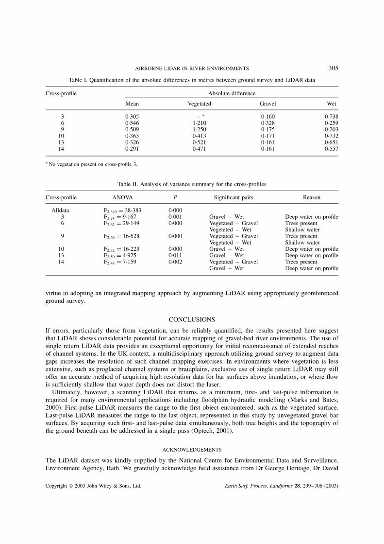
The measurement of channel cross-profiles using LiDAR and ground survey is compared in Figure 4. Severalfeatures are immediately apparent. At the time of survey, a number of mid-channel and lateral gravel barsalong with isolated sections of the banks were colonized by stands of mature Alnus glutinosa. While much ofthis has disappeared since the 1998 survey as a result of a series of major flood events, this woody vegetationis evident on the cross-section LiDAR plots as ‘spikes’ in the elevation data. No spikes are seen in the groundsurvey data as vegetation was ignored. The zones of deeper water, evident in Figure 2 as white zones, arealso replicated here as gaps in the LiDAR coverage in cross-sections 3 and 14. In addition, the nature ofthe single return measurement used here means deeper water is poorly represented in cross-sections 10 and13. Elsewhere there is reasonable correspondence between the ground and LiDAR coverages, although noconsistent pattern of superposition is apparent. The absolute differences in elevation between the LiDARand ground survey profiles are shown in Figure 4. These differences are tabulated for the different surfacecharacteristics along each profile (Table I).

It is evident that the mean difference figures exceed Fowler’s (2000) estimation of precision (15 cm); thisis due to discrepancies introduced by tall vegetation (trees) and deep water. When the figures are examinedfor the different surface characteristics, it is clear that the best correlation between LiDAR and ground surveyis provided by the gravel bar surfaces. With the exception of cross-profile 6, the figures for the gravel surfacesare consistent with Fowler’s estimation of precision.

A one-way ANOVA test is appropriate to consider whether there is sufficient evidence for these differences.Tests were carried out on the whole data set as well as each of the cross-sections and the F-tests were seen tobe significant at the 5 per cent level in all cases (Table II). However, these results only indicate that, for eachtest, at least one of the means is different from the rest. It is helpful to carry out post hoc tests to determinewhich of the three pairs of substrate means are significantly different. The results of a Scheffe test are shownin Table II for those substrate pairs which are significant at the 5 per cent level and some reasons for thesedifferences are also summarized. (The Scheffe test permits post hoc multiple comparisons between a set ofmeans; Scheffe, 1959.)

The LiDAR-generated cross-profiles are incomplete where there is deep water (e.g. cross-profile 3) anddistorted where trees are present (e.g. cross-profiles 6, 9, 13 and 15). The absolute differences from theground surface vary from 1Ð579 m (due to deep water) to 3Ð908 m (due to trees), where the degree ofdifference attributable to vegetation reflects the influence of first return data. Due to the distorting effectsof vegetation, elevation values are difficult to delineate from base topography using a single return LiDARsurvey. The LiDAR data provided by the EA trade off the frequency of measurement by the detector againstpulse separation, a problem also encountered by Marks and Bates (2000). As Marks and Bates point out, thedetector registers only the pulse returned from the terrain surface (vegetation or topography), and eliminationof vegetation effects through height differencing of the first and last returns or the full return waveform (suchas by Weltz et al., 1994) was therefore impossible. Some workers have made initial attempts to address thisby gridding the data and applying a simple variance filter (Marks and Bates, 2000); however, this approach,while appearing a reasonable initial attempt to deal with this complex issue, inevitably leads to some loss ofresolution (Marks and Bates, 2000). An alternative approach could be to use georeferenced aerial photography(if available) to distinguish and classify vegetation, permitting more vigorous elimination of LiDAR spikesin vegetated areas.

Aerial photographs have been used to estimate water depths in shallow gravel-bed rivers (e.g. Winterbottomand Gilvear, 1997; Gilvear et al., 1998), and although such an approach is limited in scope to rivers withshallow and relatively clear water, depth determination of up to one metre should be feasible with standardcolour photography. However, in this reach of the River Coquet, pools frequently exceed this threshold depth.In attempting to overcome the same problem, Irish and Lillycrop (1999) recommend using multispectrallaser imagery allowing subtraction of the difference between the reflection from the water surface of theshorter wavelengths from the longer wavelengths that can penetrate the water column. This approach permitsmeasurement of the bed surface beneath deeper water provided that associated problems with turbulenceand suspended sediment attenuating the penetration of light within a water column are not prohibitive. Suchmultispectral data were not, however, available for the River Coquet. In their absence, there is therefore a



20 40 60 80 100 120 140

20 40 60 80 100 120 140

20 40 60 80 100 120 140

20 40 60 80 100 120 140

20 40 60 80 100 120 140

20 40 60 80 100 120 140 20 40 60 80 100 120 140

20 40 60 80 100 120 140

20 40 60 80 100 120 140

20 40 60 80 100 120 140

20 40 60 80 100 120 140

20 40 60 80 100 120 140

lidar-3survey-3

Distance across channel (m)

-2

-1

2

3

1

0

-2

-1

2

3

1

0

-2

-1

2

3

1

0

-2

-1

2

3

1

0

-2

-1

2

3

1

0

-2

-1

2

3

1

0

-2

-1

2

3

1

0

-2

-1

2

3

1

0

-2

-1

2

3

1

0

-2

-1

2

3

1

0

-2

-1

2

3

1

0

-2

-1

2

3

1

0

lidar-6survey-6

lidar-9survey-9

lidar-13survey-13

lidar-14survey-14

surveydifference

surveydifference

surveydifference

surveydifference

surveydifference

Distance across channel (m)

Hei

ght a

bove

loca

l dat

um (

m)

lidar-10survey-10

surveydifference

Hei

ght a

bove

loca

l dat

um (

m)

Hei

ght a

bove

loca

l dat

um (

m)

Figure 4. Comparison between LiDAR and ground survey for six cross-sections on the River Coquet. Absolute differences betweenLiDAR and ground survey profiles are also given



Table I. Quantification of the absolute differences in metres between ground survey and LiDAR data

Cross-profile Absolute difference

Mean Vegetated Gravel Wet

3 0Ð305 – Ł 0Ð160 0Ð7386 0Ð546 1Ð210 0Ð328 0Ð2599 0Ð509 1Ð250 0Ð175 0Ð203

10 0Ð363 0Ð413 0Ð171 0Ð73213 0Ð326 0Ð521 0Ð161 0Ð65114 0Ð291 0Ð471 0Ð161 0Ð557

Ł No vegetation present on cross-profile 3.

Table II. Analysis of variance summary for the cross-profiles

Cross-profile ANOVA P Significant pairs Reason

Alldata F2,340 D 38Ð383 0Ð0003 F2,24 D 9Ð167 0Ð001 Gravel – Wet Deep water on profile6 F2,62 D 29Ð149 0Ð000 Vegetated – Gravel Trees present

Vegetated – Wet Shallow water9 F2,69 D 16Ð628 0Ð000 Vegetated – Gravel Trees present

Vegetated – Wet Shallow water10 F2,72 D 16Ð223 0Ð000 Gravel – Wet Deep water on profile13 F2,50 D 4Ð925 0Ð011 Gravel – Wet Deep water on profile14 F2,48 D 7Ð159 0Ð002 Vegetated – Gravel Trees present

Gravel – Wet Deep water on profile

virtue in adopting an integrated mapping approach by augmenting LiDAR using appropriately georeferencedground survey.

CONCLUSIONS

If errors, particularly those from vegetation, can be reliably quantified, the results presented here suggestthat LiDAR shows considerable potential for accurate mapping of gravel-bed river environments. The use ofsingle return LiDAR data provides an exceptional opportunity for initial reconnaissance of extended reachesof channel systems. In the UK context, a multidisciplinary approach utilizing ground survey to augment datagaps increases the resolution of such channel mapping exercises. In environments where vegetation is lessextensive, such as proglacial channel systems or braidplains, exclusive use of single return LiDAR may stilloffer an accurate method of acquiring high resolution data for bar surfaces above inundation, or where flowis sufficiently shallow that water depth does not distort the laser.

Ultimately, however, a scanning LiDAR that returns, as a minimum, first- and last-pulse information isrequired for many environmental applications including floodplain hydraulic modelling (Marks and Bates,2000). First-pulse LiDAR measures the range to the first object encountered, such as the vegetated surface.Last-pulse LiDAR measures the range to the last object, represented in this study by unvegetated gravel barsurfaces. By acquiring such first- and last-pulse data simultaneously, both tree heights and the topography ofthe ground beneath can be addressed in a single pass (Optech, 2001).

ACKNOWLEDGEMENTS

The LiDAR dataset was kindly supplied by the National Centre for Environmental Data and Surveillance,Environment Agency, Bath. We gratefully acknowledge field assistance from Dr George Heritage, Dr David



Passmore and Dr David Milan. We also thank Mr Brian Little and Mr Guy Renwick for granting access tothe site. Comments from three referees are gratefully acknowledged.

REFERENCES

Bissonnette LR, Kunz G, WeissWrana K. 1997. Comparison of LiDAR and transmissometer measurements. Optical Engineering 36:131–138.

Brasington J, Rumsby BT, McVey RA. 2000. Monitoring and modelling morphological change in a braided gravel-bed river using highresolution GPS-based survey. Earth Surface Processes and Landforms 25: 973–990.

Brinkman RF, O’Neill C. 2000. LiDAR and photogrammetric mapping. The Military Engineer May-June.Environment Agency. 1998. Local Environment Agency Plan: Cheviot and East Northumberland Action Plan . North East Region,

Newcastle upon Tyne.Ferguson RI, Werritty A. 1983. Bar development and channel changes in the gravelly River Feshie. In Modern and Ancient Fluvial

Systems , Collinson JD, Lewin J (eds). International Association of Sedimentologists, Special Publication 6: 133–143.Fowler A. 2000. The lowdown on LiDAR. Earth Observation Magazine 7: 227.Fuller IC, Passmore DG, Heritage GL, Large ARG, Milan DJ, Brewer PA. 2002. Annual sediment budgets in an unstable gravel bed

river: the River Coquet, northern England. In: Sediment Flux to Basins: Causes, Controls and Consequences , Jones S, Frostick LE(eds). Geological Society, Special Publication 191; 115–131.

Gauldie RW, Sharma SK, Helsley CE. 1996. LiDAR applications to fisheries monitoring problems. Canadian Journal of Fisheries andAquatic Sciences 53: 1459–1467.

Gilvear DJ, Waters TM, Milner AM. 1998. Image analysis of aerial photography to quantify the effect of gold placer mining on channelmorphology, Interior Alaska. In Landform Monitoring, Modelling and Analysis , Lane SN, Richards KS, Chandler JH (eds). Wiley:Chichester; 195–216.

Innes JL, Koch B. 1998. Forest biodiversity and its assessment by remote sensing. Global Ecology and Biogeography Letters 7: 397–419.Irish JL, Lillycrop WJ. 1999. Scanning laser mapping of the coastal zone: the SHOALS system. ISPRS Journal of Photogrammetry and

Remote Sensing 54: 123–129.Irish JL, White TE. 1998. Coastal engineering applications of high-resolution LiDAR bathymetry. Coastal Engineering 35: 47–71.Jackson TJ, Ritchie JC, White J, Leschack L. 1988. Airborne laser profile data for measuring ephemeral gully erosion. Photogrammetric

Engineering and Remote Sensing 54: 1181–1185.Krabill W, Thomas R, Jasek K, Kuvinen K, Manizade S. 1995. Greenland ice thickness changes measured by laser altimetry.

Geophysical Research Letters 22: 2341–2344.Marks K, Bates P. 2000. Integration of high-resolution topographic data with floodplain flow models. Hydrological Processes 14:

2109–2122.McHenry JR, Cooper CM, Ritchie JC. 1982. Sedimentation in Wolf Lake, Lower Yazoo river basin, Mississippi. Journal of Freshwater

Ecology 1: 547–558.Optech. 2001. http://www.optech.on.ca/aboutlaser.htm.Parson LE, Lillycrop WJ, Klein CJ, Ives RCP, Orlando SP. 1997. Use of LiDAR technology for collecting shallow water bathymetry

of Florida Bay. Journal of Coastal Research 13: 1173–1180.Press WH, Flannery BP, Teukolsky SA, Vetterling WT. 1989. Numerical Recipes in Pascal . Cambridge University Press: Cambridge.Ritchie JC, Jackson TJ. 1989. Airborne laser measurements of the surface-topography of simulated concentrated flow gullies.

Transactions of the ASAE 32: 645–648.Ritchie JC, Everitt JH, Escobar DE, Jackson TJ, Davis MR. 1992. Airborne laser measurements of rangeland canopy cover and

distribution. Journal of Range Management 45: 189–193.Ritchie JC, Grissinger EH, Murphey EB, Garbrecht JD. 1994. Measuring channel and gully cross-sections with an airborne laser

altimeter. Hydrological Processes 8: 237–243.Ritchie JC, Humes KS, Weltz MA. 1995. Laser altimeter measurements at Walnut-Gulch watershed, Arizona. Journal of Soil and Water

Conservation 50: 440–442.Ritchie JC, Menentie M, Weltz MA. 1996. Measurements of land surface features using an airborne laser altimeter: the HAPEX-Sahel

experiment. International Journal of Remote Sensing 17: 3705–3724.Scheffe H. 1959. The Analysis of Variance. Wiley: New York.Wadhams P. 1995. Arctic sea-ice extent and thickness. Philosophical Transactions of the Royal Society of London Series A 352: 301–319.Weltz MA, Ritchie JC, Fox HD. 1994. Comparison of laser and field-measurements of vegetation height and canopy cover. Water

Resources Research 30: 1311–1319.Westaway RM, Lane SN, Hicks DM. 2000. The development of an automated correction procedure for digital photogrammetry for the

study of wide, shallow gravel-bed rivers. Earth Surface Processes and Landforms 25: 209–226.Winterbottom SJ, Gilvear DJ. 1997. Quantification of channel bed morphology in gravel-bed rivers using airborne multispectral imagery

and aerial photography. Regulated Rivers: Research & Management 13: 489–499.


application of airborne lidar in river environments: the...

Documents