application of active magnetic force actuator for control
TRANSCRIPT
Cleveland State University Cleveland State University
EngagedScholarship@CSU EngagedScholarship@CSU
ETD Archive
2011
Application of Active Magnetic Force Actuator for Control of Application of Active Magnetic Force Actuator for Control of
Flexible Rotor System Vibrations Flexible Rotor System Vibrations
Volodymyr Mykhaylyshyn Cleveland State University
Follow this and additional works at: https://engagedscholarship.csuohio.edu/etdarchive
Part of the Mechanical Engineering Commons
How does access to this work benefit you? Let us know! How does access to this work benefit you? Let us know!
Recommended Citation Recommended Citation Mykhaylyshyn, Volodymyr, "Application of Active Magnetic Force Actuator for Control of Flexible Rotor System Vibrations" (2011). ETD Archive. 664. https://engagedscholarship.csuohio.edu/etdarchive/664
This Thesis is brought to you for free and open access by EngagedScholarship@CSU. It has been accepted for inclusion in ETD Archive by an authorized administrator of EngagedScholarship@CSU. For more information, please contact [email protected].
APPLICATION OF ACTIVE MAGNETIC FORCE ACTUATOR FOR
CONTROL OF FLEXIBLE ROTOR SYSTEM VIBRATIONS
VOLODYMYR MYKHAYLYSHYN
Master of Science in
Mechanical Engineering
Ternopil Ivan Pul’uj National Technical University
June, 2001
submitted in partial fulfillment of requirements for the degree
MASTER OF SCIENCE
IN MECHANICAL ENGINEERING
at the
CLEVELAND STATE UNIVERSITY
October, 2011
This thesis has been approved
for the Department of MECHANICAL ENGINEERING
and the College of Graduate Studies by
Dr. Jerzy T. Sawicki, Thesis Committee ChairpersonDepartment of Mechanical Engineering, CSU
Dr. Stephen F. DuffyDepartment of Civil and Environmental Engineering, CSU
Dr. Taysir H. NayfehDepartment of Mechanical Engineering, CSU

ACKNOWLEDGMENT
I would like to express my heartfelt gratitude to Dr. Jerzy T. Sawicki for his patient
understanding, goodness, and guidance through my graduate career. By teaching me to
do things right, he changed me and my life. Without his constant support, helpful
discussions, and motivation during my education, this thesis would not have been
possible.
I would like to thank Dr. Taysir H. Nayfeh and Dr. Stephen F. Duffy, who served on
the thesis committee for their consideration, time, and evaluation.
Also I appreciate my lab mate Alexander Pesch for his encouragement and time we
spent discussing different problems.
I am grateful to my family for believing in me and support through years of my
education.
iv
APPLICATION OF ACTIVE MAGNETIC FORCE ACTUATOR FOR CONTROL OF
FLEXIBLE ROTOR SYSTEM VIBRATIONS
VOLODYMYR MYKHAYLYSHYN
ABSTRACT
The purpose of this work was to develop and experimentally demonstrate a novel
approach to minimize lateral vibrations of flexible rotor. The applied feed forward
control approach employed magnetic force actuator to inject a specially designed force to
counteract the rotor unbalance force. By specific selection of frequency and phase as
functions of the rotor running speed and rotor natural frequency, the proposed simplified
injection waveform has been shown to be effective both in reducing the rotor’s vibrations
and for hardware implementation. A model of the test rig was constructed using the
finite element (FE) method and was validated using experimental data. The effectiveness
of the proposed current injection was numerically simulated with FE model and
experimentally validated using a residual unbalance force. It was noticed that at a
selected constant running speed, just below the first rotor critical speed, the rotor
vibrations were reduced approximately by 90%. The method was also implemented
during the speed ramp test, which passes through the first critical speed. In this test the
proposed force injection also reduced vibrations at various rotor speeds. These results
agree well with the results of simulation.
v
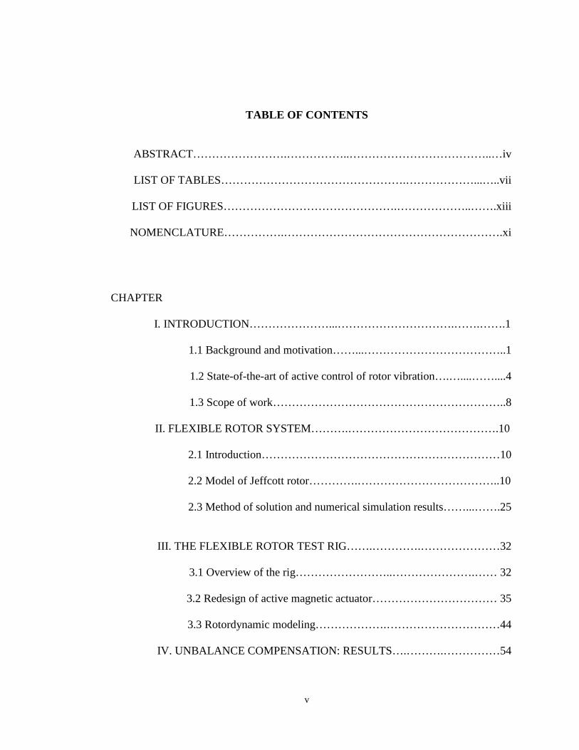
TABLE OF CONTENTS
ABSTRACT…………………….……………..………………………………..…iv
LIST OF TABLES………………………………………….………………...…..vii
LIST OF FIGURES……………………………………….………………..…….xiii
NOMENCLATURE…………….………………………………………………….xi
CHAPTER
I. INTRODUCTION…………………...………………………….…….…….1
1.1 Background and motivation……...………………………………..1
1.2 State-of-the-art of active control of rotor vibration….…....……....4
1.3 Scope of work……………………………………………………..8
II. FLEXIBLE ROTOR SYSTEM……….………………………………….10
2.1 Introduction………………………………………………………10
2.2 Model of Jeffcott rotor………….………………………………..10
2.3 Method of solution and numerical simulation results……...…….25
III. THE FLEXIBLE ROTOR TEST RIG…….………….…………………32
3.1 Overview of the rig……………………..………………….…… 32
3.2 Redesign of active magnetic actuator…………………………… 35
3.3 Rotordynamic modeling……………….…………………………44
IV. UNBALANCE COMPENSATION: RESULTS….……….……………54
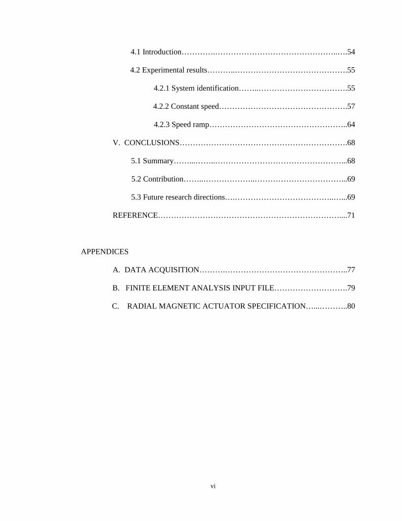
vi
4.1 Introduction………….………………………………………..….54
4.2 Experimental results………..…………………………………….55
4.2.1 System identification……..…………………………….55
4.2.2 Constant speed………………………………………….57
4.2.3 Speed ramp……………………………………………..64
V. CONCLUSIONS……………………………………………………….68
5.1 Summary……...……..…………………………………………...68
5.2 Contribution……..………………..……………………………...69
5.3 Future research directions….………………………………..…...69
REFERENCE……………………………………………………………....71
APPENDICES
A. DATA ACQUISITION……….………………………………………..77
B. FINITE ELEMENT ANALYSIS INPUT FILE……………………….79
C. RADIAL MAGNETIC ACTUATOR SPECIFICATION…...………..80
vii
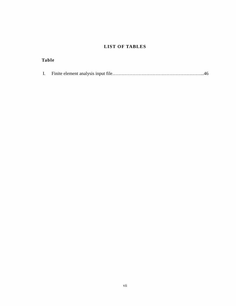
LIST OF TABLES
Table
I. Finite element analysis input file…………………………………………………...46
viii
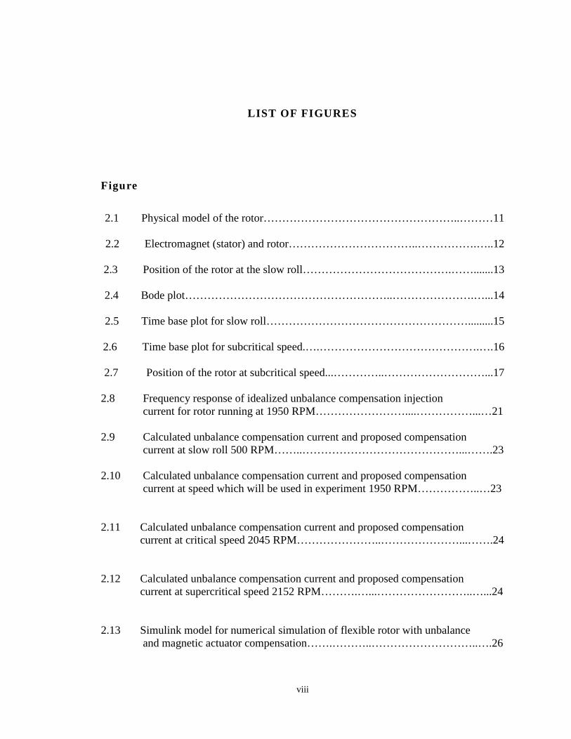
LIST OF FIGURES
Figure
2.1 Physical model of the rotor……………………………………………..………11
2.2 Electromagnet (stator) and rotor……………………………..…………….…..12
2.3 Position of the rotor at the slow roll………………………………….…….......13
2.4 Bode plot………………………………………………..………………….…...14
2.5 Time base plot for slow roll……………………………………………….........15
2.6 Time base plot for subcritical speed.….…………………………………….….16
2.7 Position of the rotor at subcritical speed...…………..………………………...17
2.8 Frequency response of idealized unbalance compensation injectioncurrent for rotor running at 1950 RPM……………………....……………...…21
2.9 Calculated unbalance compensation current and proposed compensationcurrent at slow roll 500 RPM……..……………………………………...…….23
2.10 Calculated unbalance compensation current and proposed compensationcurrent at speed which will be used in experiment 1950 RPM……………..…23
2.11 Calculated unbalance compensation current and proposed compensationcurrent at critical speed 2045 RPM…………………..…………………...…….24
2.12 Calculated unbalance compensation current and proposed compensationcurrent at supercritical speed 2152 RPM……….…...……………………..…...24
2.13 Simulink model for numerical simulation of flexible rotor with unbalanceand magnetic actuator compensation…….………..………………………..….26
ix
2.14 Simulink model of magnetic actuator force corresponding to block“MA x axis” shown in Figure2.8………..…....………………..……………....27
2.15 Sample of current signals sent to magnetic actuator in simulation……………28
2.16 Simulated vibration of rotor at disk in horizontal and vertical directionswith no vibration control….……………………..…………………………….29
2.17 Simulated vibration of rotor at disk in horizontal and vertical directionswith vibration control……………………………………………………….…30
2.18 Simulated rotor orbit at the disk with vibration control (left) and withno control (right)………..……………………………………………………..31
3.1(a) Bently Nevada rotor kit RK4 with active magnetic actuator…………...……..33
3.1(b) Active magnetic actuator…………………………….…...…………………...33
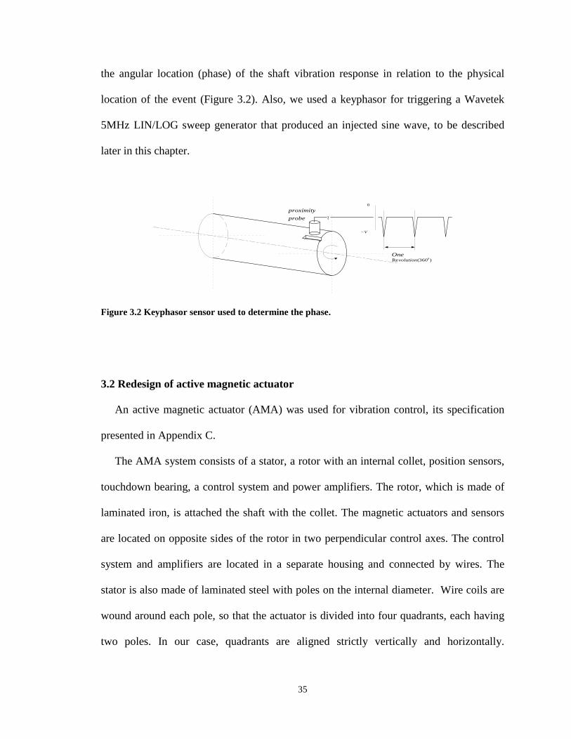
3.2 Keyphasor……..…………………………………………………………...….35
3.3 Components of the active magnetic actuator……….…………………………37
3.4 V-shape actuators mount…….……….…………………...…………………...38
3.5 V-shape base schemes……..…………………………………………………..38
3.6 Active magnetic actuator assembled on V-shape base….………..……….......39
3.7 Scheme of connection of the rig………...……………………..……………...40
3.8 Finite element model of rotor…..……………..…………………..………......45
3.9 Campbell diagram for rotor…………..……………………………………….47
3.10 Undamped critical speed map………………………………..………………..48
3.11 First natural mode shape at 33.4 Hz……………………………………….......49
3.12 Second natural mode shape at 126.6 Hz…….………………………………...50
3.13 Rotordynamic response plot at the location of the rotor ofthe active magnetic actuator……...………………………………….……..….51
3.14 Rotordynamic response plot at the location of theADRE horizontal proximity probe…………………………….………….…...52

x
3.15 Rotordynamic response plot at the location of the verticalADRE proximity probe………….………………………….…………..……..53
4.1 Hewlett Packard 35670A dynamic signal analyzer…….…..………….……...56
4.2 Transfer function of the experimental …..……..………..…………...57
4.3 Response of the shaft and generated current………..…………………………58
4.4 Numerical data of the response and current……..………………………….....59
4.5 Orbit of the shaft without injection…………..………………………………..60
4.6 Response of the shaft and injected current…………..……………...………...61
4.7 Response of the shaft and injected current (numerical view)…….………….61
4.8 Response of the shaft with injection………………….………………………62
4.9 Orbit of the shaft (a) with current injection,b)without current injection…………….……………………………….……..63
4.10 Experimental Bode plot (no injection)……….…………………….…………64
4.11 Experimental Bode plot of the rotor with injected force……...………...……65
4.12 Response of the rotor at the speed range with and withoutforce injection……...…….…..……………………...………………………..66
xi
NOMENCLATURE
angular velocity
M mass of the disk
J polar moment of inertia with respect to the axis of rotation
m center of mass (heavy spot)
l distance between center of mass and geometrical center of the disk (eccentricity)
r radius of the shaft
O geometrical center of the disk
0O position of the geometrical center of the disk without rotation
1O position of the geometrical center of the disk at “slow roll”
2O position of the geometrical center of the disk at subcritical speed
angular position of the center of mass measured from the reference angle zero
angular position of the high beat point measured from the reference angle zero
angel between center of mass and respond spot (phase)
0 angel between center of mass and respond spot (phase) at “slow roll”
2 angel between center of mass and respond spot (phase) at subcritical speed
3 angel between center of mass and respond spot (phase) at post critical speed
F unbalance (exciting) force
aF attractive magnetic force
1F attractive magnetic force at the location of the center of mass
xii
2F attractive magnetic force at the location of the high spot
geometric correction factor
0 permeability of free space
gA single pole face area
N total number of wire coils in a horseshoe
I current in the coil
g air gap distance between rotor and stator
staticg nominal air gap distance between rotor and stator
1g air gap distance between rotor and stator at the location of the center of mass
0g air gap distance between rotor and stator at “slow roll”
2g air gap distance between rotor and stator at subcritical speed
3g air gap distance between rotor and stator at post critical speed

1
CHAPTER I
INTRODUCTION
1.1 Background and Motivation.
The dynamic of rotating systems was well understood long time ago thanks to number
of mathematicians and theoretical mechanics. Beginning with the ancient world we can
observe that scientist showed interest in harmonic motion and vibration. Pythagoreans
determined the natural frequency of vibrating system and proved that it is a property of
the system in the V century B.C. and Aristotle (384 – 322 B.C.) developed a fundamental
understanding of statics and dynamics. Also, archeologists discovered that ancient
Chinese scientists invented seismograph, which was used to measure earthquakes.
The modern day theory was probably founded by scientists and mathematicians such
Sir Isaac Newton (1642–1737), who gave us calculus and the laws of motion for
analyzing vibration; Daniel Bernoulli (1700 – 1782) and Leonard Euler (1707 – 1783)
who studied beam vibrations (Bernoulli – Euler beam); and Josef Fourier (1768 – 1830),
2
who developed the theory of frequency analysis of signals. The technological revolution
expanded our present engineering development toward higher speeds and heavier loads
on machines, involving higher dynamic stresses caused by increased mechanical
vibrations. Proper design and control are crucial in maintaining high performance level
and production efficiency, and prolonging the useful life of machinery, structures and
industrial processes. The reliability of machines with rotating parts is closely connected
with the vibrational characteristic of the rotor as a whole and of its elements and with the
maintenance of the permissible level of vibrational stress. Rotordynamic dates from the
second half of the nineteenth century. The first systematic work was written by Lord
Rayleigh [24] where he introduced a correction to the lateral vibration of the beam due to
rotor inertia. Timoshenko [29] presented a model that takes into account shear
deformation and rotational inertia effects. Whirling of shafts was investigated by W.A.
Rankine [22], who anticipated that shaft operation above critical speed is impossible. The
first successful rotor model was proposed by Föppl in 1895. He described a single disk
centrally located on a circular shaft, without damping and demonstrated that supercritical
operation was stable [8]. Significant work was done by De Laval. His analysis was
inaccurately credited to Jeffcott who published his similar work in a widely read English
journal [11]. Later the Soviet scientists Nikolai [20] examined the stability of the shaft
with a disk mounted in the centre, and the stability of a shaft with the disk attached to the
free end. P.L. Kapitsa pointed out that a flexible shaft could become unstable due to
friction condition in its sliding bearings [12]. Many rotordynamics textbooks were
created, for example, by J.M. Vance [29], Erwin Kramer “Dynamics of Rotors and
Foundations” [15], K. Czolczynski [3] discussed aspects affecting the stability of the
3
system, “Handbook of Rotordynamic” by Frederic F Ehrich [6] reflect devices and
phenomena which have entered the practice of rotordynamics engineering. A. Muszynska
[18] at her “Fundamental Response of a Rotor” discussed rotor response to the inertia
force due to unbalance. J.T. Sawicki [25] at “Unbalance Response Prediction for
Accelerating Rotors with Load-Dependent Nonlinear Bearing Stiffness” discussed
unbalance response for an accelerating rotor supported on ball bearings. Many other great
scientists made their contributions in the study of dynamics of rotating machinery.
The new chapter in these investigations began with the appearance of magnetic
actuators, which allow unique application of rotating machinery with excellent
performance. Magnetic actuator is typical mechatronics product; it is composed of
mechanical and electronic elements. The properties and principles of work will be
described in Chapter III. The study of magnetic levitation goes back to S. Earnshaw [5].
Earnshaw’s theorem contends that if inverse square law forces control a flow of charged
particles, they can never be stable. The theorem is based on the Laplace partial
differential equation. The solution of this equation does not have any local maxima or
minima, so there can be no equilibrium. This theorem confirms that it is impossible to
have a completely stable system using only forces of static fields of permanent magnets.
The next level of investigation of properties of magnetic actuators was begun in the
early forties of the nineteenth century when early magnetic bearing patents were assigned
to Jesse Beam. This technology matured with the work of H. Habermann [10] and G.
Schweitzer [26], where they developed modern computer-based control technology. A
great number of scientists made their contributions to the science of vibration control.
4
Many different methods and techniques were proposed. Some of them, which are of
interest of this work, will be introduced.
1.2 State-of-the-Art of Active Control of Rotor Vibration.
A major problem faced by rotating machinery is the imbalance induced vibration. The
flexible rotor may have a variety of unbalance distribution. According to F. Ehrich [6]
there are four basic types of unbalance distribution encountered with multimass rotor.
First, continuous unbalance distribution along the shaft. The second distribution includes
radial unbalances, such as encountered by assembled compressor turbine stages on a
shaft. The third distribution represents a shaft with bow. In a bowed rotor the principal
axis of inertia (centerline) of the rotor is not concurrent with its axis of rotation. Bows
may be introduced by no uniform shrink fits, thermal effects, and permanent sag due to
gravitational effects. Fourth is the disk skew. Usually, not only one type of unbalance
appears.
There are great number of methods that can be applied to compensate this unbalance
[30]. Generally, they can be divided into two main categories: passive and active. In the
passive method we ‘assign’ balancing weights and select proper operational speed.
Balancing can be done by different methods such as single-plane balancing by influence
coefficient method, two-plane balancing by the influence coefficient method, single-
plane balancing using static and dynamic components, single-plane balancing by the
influence coefficient method using linear regression, generalized influence coefficient
method using pseudo-inversion, multiplane balancing using linear programming
5
techniques, modal balancing, three-trial-weight method of balancing, multiplane
balancing without phase, rotor balancing without trial weights, coupling trim balancing
and other [6]. All of the methods can be divided into two categories: modal methods and
influence coefficient methods. The modal method, based on a rotating structure model,
determines experimentally the disturbing unbalance associated with a specific mode. The
influence coefficient method uses experimental models that represent the machine’s
sensitivity to unbalances. Some of them are very interesting but others are expensive and
time-consuming. The conditions where these methods can be effective are limited and
even though the rotor amplitude may be reduced to small vibrations at the particular
location and speed, other points along the rotor may exhibit higher vibrations. At other
speeds the rotor may appear not be in balance.
Active methods for vibration control in rotors involve controlled force delivered by
actuators. There are different types of actuators such as hydraulic, pneumatic,
piezoelectric, and electromagnetic. The advantage of electromagnetic actuators will be
described later. Considerable research has already been done on design and application of
magnetic actuators [6].
Kari Tammi [28] created a control system for active vibration control of rotor on
similar, to presented in this thesis, test environments. He designed controllers using
feedback and feedforward control algorithm. This control system determines the force
required and applies the force commands to the force control system. The control system
design was based on knowledge available about the system to be controlled, and the
parameters were assumed invariant in time. However, the higher peaks were observed at
post critical rotational speed. The clear explanation for this behavior was not presented.
6
The study confirms that reductions in rotor’s response can be achieved by compensating
the disturbance by means of the reference signal.
M.E.F. Kasarda [13] proposed active control solution utilizing active magnetic bearing
(AMB) technology in conjunction with conventional support bearings. The AMB is
utilized as an active magnetic damper (AMD) at rotor locations inboard of conventional
support bearings. Another active magnetic actuator was used as a source of sub
synchronous vibration. The study shows that sub synchronous vibrations are reducible
with an AMD. The study also shows that the AMD can significantly increase
synchronous vibration response (up to 218%) by increasing system stiffness. The overall
results from this work demonstrate that full rotor dynamic analysis and design are critical
for successful application of this approach.
J.M. Krodkiewski at the University of Melbourne used active hydrodynamic bearing
as a third bearing to add damping to the system. A multivariable adaptive self tuning
regulator was used to control oil film thickness in the third bearing located between the
load carrying ball bearings. The system was designed to cope with non-linear fluid-film
bearing characteristics, parameter vibrations and parameter uncertainty. [16].
Interesting results were shown in “Active Balancing of Turbo machinery: Application
to Large Shaft Lines” by C. Alauze [1]. The unbalance correction was carried out in real
time, during operation in steady state and transient responses. The concept consists of
generating a correction force by using two mobile weights situated in the same plane and
running at a constant radius of the rotation axis. The balancing process is based on the
influence coefficient method and includes specific measurement and control
developments. The behavior (Bode plot) of the heavy 5.56m long, 110 to 360 mm
7
diameter and disk with mass 4.3 tons that situated in the middle was very similar to the
behavior of the test rig used at present work.
An interesting method was established by C.R. Knospe [14]. The stability and
performance robustness of an adaptive open loop control algorithm was examined.
Expressions were derived for a number of unstructured uncertainties. The experimental
results indicate that the theoretical expressions do provide an upper bound on actual
performance however, this bound is not tight.
Robust modal control design of a magnetically suspended rotor was presented in a
simulation study by Hsiang-Chieh Yu [31], involving the finite element formulation. The
original system is augmented using the direct output control in the first level, which
removes the repeated rigid body modes of an uncontrolled system. In the second level
design, a robust controller is implemented in the complex modal space. It has been
theoretically shown that the presented control design is robust, but not proved
experimentally.
M.S. De Querioz [22] presents the active feedback method that asymptotically learns
the unbalance-induced disturbance forces and identifying the unknown unbalance-related
parameters of a rotor.
A new approach was proposed by Kai-Yew Lum [17] that differs from the usual
adaptive feed-forward compensation. Under the proposed control law, a rigid rotor
achieves rotation about the mass center and principal axis of inertia. The calculation and
simulation example was done for a rotor supported by two AMBs.
Another good experiment in a similar test environment was done by C.R. Burrows [2]
at the University of Bath. In their work “Design and Application of a Magnetic Bearing
8
for Vibration Control and Stabilization of a Flexible Rotor” they described using a
magnetic actuator, control algorithm that determines the amplitude and phase required for
each axis and some typical optimum control forces obtained experimentally.
Various active control techniques, applicable to rotating machinery where, presented
in work, performed by Heinz Ulbrich [29]. In his “Elements of Active Vibration Control
for Rotating Machinery”, he presented several topics such as the availability of an
appropriate actuator, modeling of the entire system, positioning of actuators and sensors,
control concepts that should be used, controllability and observability. Real applications
were presented as examples.
1.3 Scope of Work
This work is concerned with the subject of vibrations, system dynamics, magnetic
actuators and their combinations. To reduce vibrations of the rotor focus was on
synchronous response due to unbalance. Unbalance is one of the most common
malfunction of rotating machines; analysis of rotor synchronous response allows to
balance the rotor; to understand more complex rotor dynamic behavior caused by various
other malfunctions, knowledge of rotor unbalance response is necessary. In order to
reduce vibrations, the design of magnetic force actuator was completed (Chapter III) and
experimentally verified.
In Chapter II, review of flexible rotor system is presented concerning to application of
active magnetic actuator. Also, finite element model of the rotor and methods of solution
were described.

9
A description of the , as well as unique features of active magnetic force actuators and
its modifications will be presented in Chapter III.
Unbalance compensation experimental results for sub and super-critical speeds with
model identification and force injection are shown in Chapter IV.
Chapter V provides conclusions as well as contributions and a short summary of future
research directions.
10
CHAPTER II
FLEXIBLE ROTOR SYSTEM
2.1 Introduction
“Everything should be made as simple as possible, but not simpler.”- Albert Einstein.
The Jeffcott rotor has a flexible mass shaft, one rigid disk at the midspan and simple
supports as bearings. The Jeffcott rotor model is obviously an over-simplification of real-
world rotors but, it helps to understand many features of real-world rotor behavior,
including critical speeds, response to unbalance, or the effect of damping.
2.2 Model of Jeffcott rotor
Consider the case of a long and lightweight shaft, rotating with an angular velocity
and carrying at its midspan a disk of mass M and mass polar moment of inertia with
respect to the axis of rotation J . As discussed in the previous chapter, a real flexible rotor
may have a variety of unbalance distributions. So, it is assumed that this is just a point
mass or heavy spot m on the disc. This unbalance heavy spot m is located at some
distance l from the geometrical center of the discO . This distance l is the disc
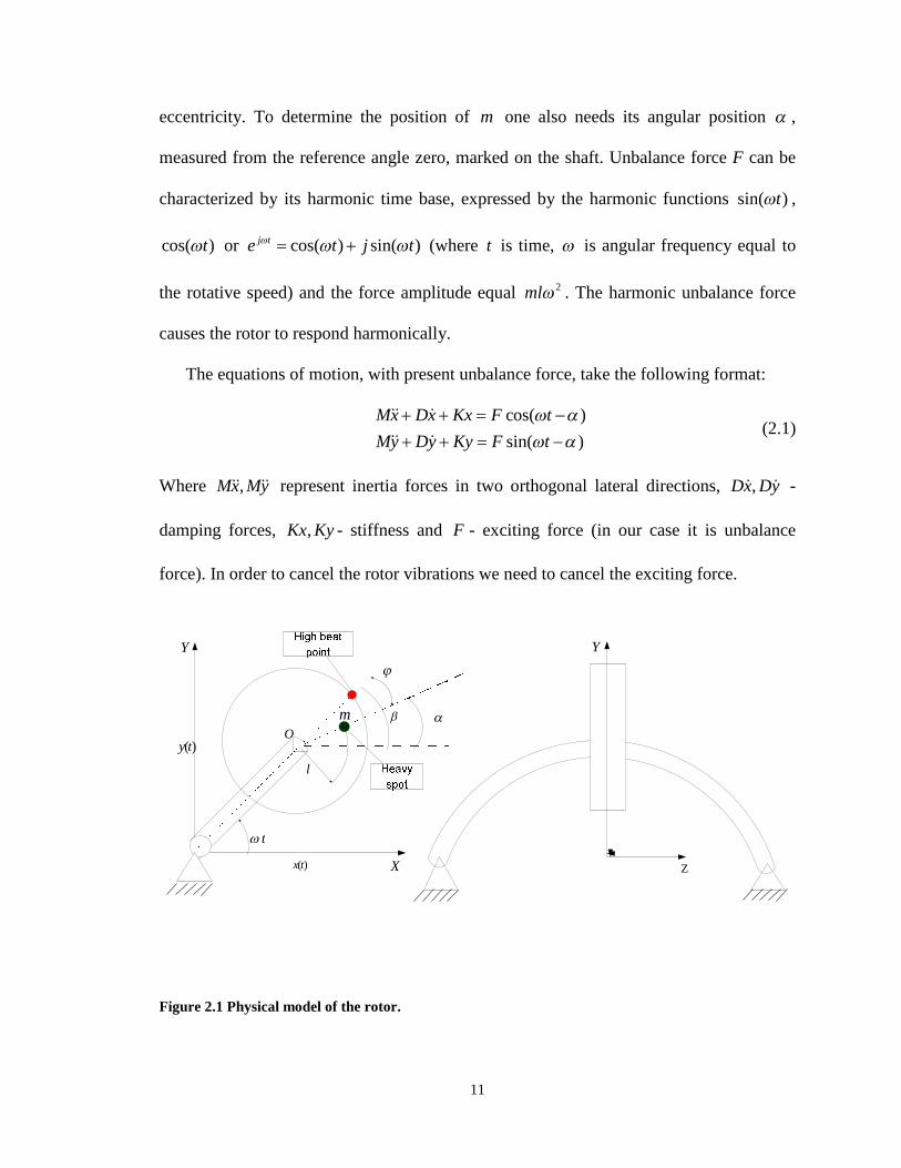
11
eccentricity. To determine the position of m one also needs its angular position ,
measured from the reference angle zero, marked on the shaft. Unbalance force F can be
characterized by its harmonic time base, expressed by the harmonic functions sin( )t ,
cos( )t or cos( ) sin( )j te t j t (where t is time, is angular frequency equal to
the rotative speed) and the force amplitude equal 2ml . The harmonic unbalance force
causes the rotor to respond harmonically.
The equations of motion, with present unbalance force, take the following format:
cos( )
sin( )
Mx Dx Kx F t
My Dy Ky F t
(2.1)
Where ,Mx My represent inertia forces in two orthogonal lateral directions, ,Dx Dy -
damping forces, ,Kx Ky - stiffness and F - exciting force (in our case it is unbalance
force). In order to cancel the rotor vibrations we need to cancel the exciting force.
Figure 2.1 Physical model of the rotor.
Z)(tx
( )y t
t
l
m
X
Y Y
O
12
Cancellation of the exciting force is possible by applying the same harmonic force but
in opposite direction. As an instrument to do this an active magnetic actuator (AMA) was
chosen.
An active magnetic actuator is a mechatronic device that uses electromagnetic fields
to apply forces to a rotor without contact. The advantages of using active magnetic
actuators are already well known. Their very low friction, virtually limitless life,
insensitivity to surrounding environment and relatively large changes in temperature, and
flexibility due to digital computer control, gives them extraordinary versatility. The
effectiveness of the active magnetic actuators is based on the nature phenomena of
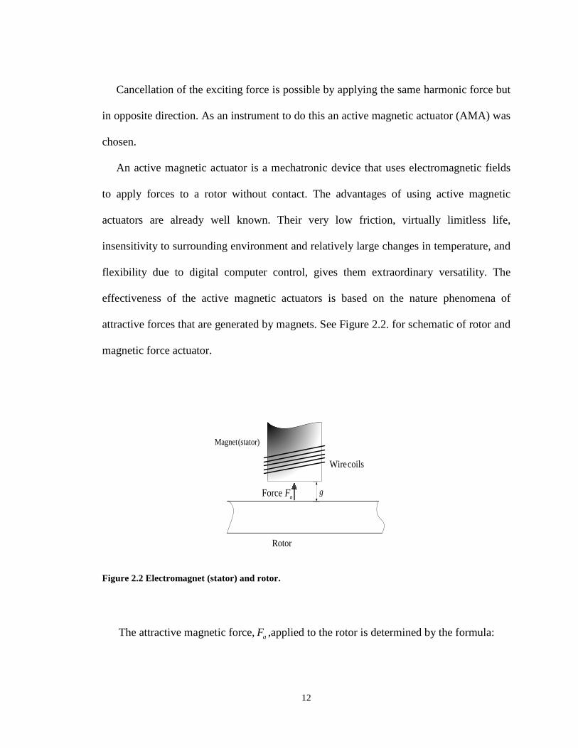
attractive forces that are generated by magnets. See Figure 2.2. for schematic of rotor and
magnetic force actuator.
g
coilsWire
aFForce
(stator)Magnet
Rotor
Figure 2.2 Electromagnet (stator) and rotor.
The attractive magnetic force, aF ,applied to the rotor is determined by the formula:
13
2 20
24
g
a
A N IF
g
(2.1)
where is a geometric correction factor, 0 is the permeability of the air gap, gA is a
single pole face area, N is the total number of wire coils in a horseshoe, I is the current
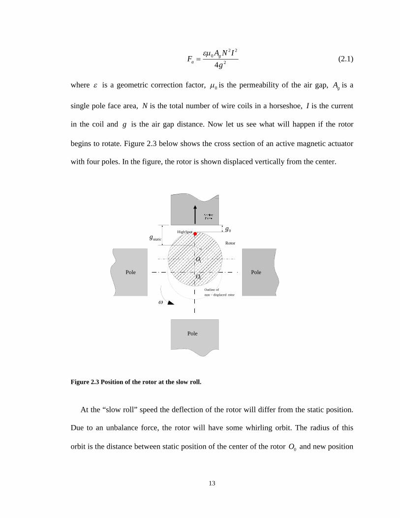
in the coil and g is the air gap distance. Now let us see what will happen if the rotor
begins to rotate. Figure 2.3 below shows the cross section of an active magnetic actuator
with four poles. In the figure, the rotor is shown displaced vertically from the center.
0g
staticg
1O
0OPole
SpotHigh
Rotor
rotordisplacednon
ofOutline
Pole
Pole
Figure 2.3 Position of the rotor at the slow roll.
At the “slow roll” speed the deflection of the rotor will differ from the static position.
Due to an unbalance force, the rotor will have some whirling orbit. The radius of this
orbit is the distance between static position of the center of the rotor 0O and new position

14
of the geometrical center of the rotor O , plus the radius of the rotor. The position of the
center of mass (heavy spot) and response point (high spot) is on the same radial line
(Figure 2.3). There is no angle between them, 0 0 .
On the Bode plot, shown in Figure 2.4, this position can be seen on the left side of the
graph (low speed).
20
3
0g
2g
3g
speed,Rotating
P
hase
,A
Am
pli
tud
e,
Figure 2.4 Bode plot of the rotor.
On the schematic Bode plot, the line that shows the position of the heavy spot has a
fixed location on the rotor. The line of the response spot (or high spot) shows that it
increases with the increased rotating speed. Also, the magnitude of vibration of the
geometrical center of the rotor grows as resonance is approached. So, to cancel the
15
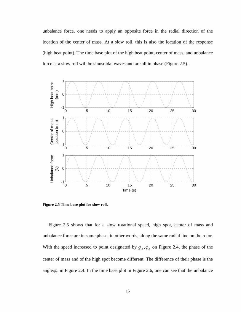
unbalance force, one needs to apply an opposite force in the radial direction of the
location of the center of mass. At a slow roll, this is also the location of the response
(high beat point). The time base plot of the high beat point, center of mass, and unbalance
force at a slow roll will be sinusoidal waves and are all in phase (Figure 2.5).
0 5 10 15 20 25 30-1
0
1
Hig
hbeat
poin
t(m
m)
0 5 10 15 20 25 30-1
0
1
Cente
rof
mass
positio
n(m
m)
0 5 10 15 20 25 30-1
0
1
Time (s)
Unbala
nce
forc
e(N
)
Figure 2.5 Time base plot for slow roll.
Figure 2.5 shows that for a slow rotational speed, high spot, center of mass and
unbalance force are in same phase, in other words, along the same radial line on the rotor.
With the speed increased to point designated by g 2 , 2 on Figure 2.4, the phase of the
center of mass and of the high spot become different. The difference of their phase is the
angle 2 in Figure 2.4. In the time base plot in Figure 2.6, one can see that the unbalance
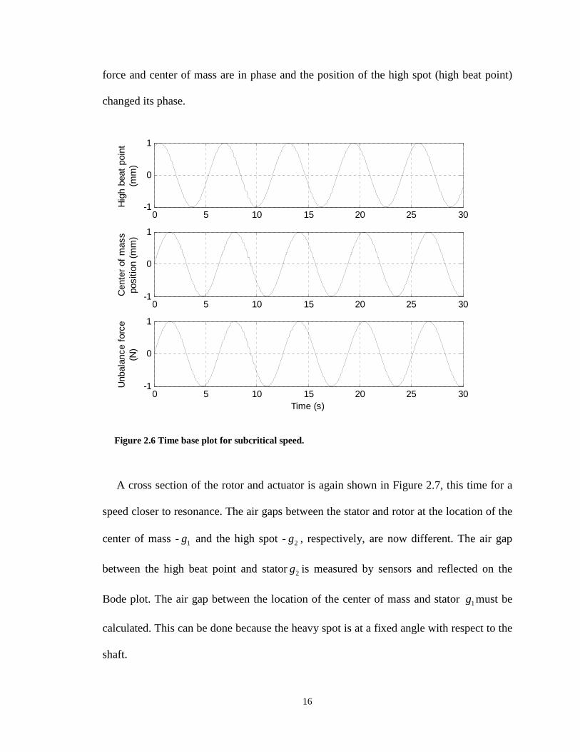
16
force and center of mass are in phase and the position of the high spot (high beat point)
changed its phase.
0 5 10 15 20 25 30-1
0
1
Hig
hbeat
poin
t(m
m)
0 5 10 15 20 25 30-1
0
1
Cente
rof
mass
positio
n(m
m)
0 5 10 15 20 25 30-1
0
1
Time (s)
Unbala
nce
forc
e(N
)
Figure 2.6 Time base plot for subcritical speed.
A cross section of the rotor and actuator is again shown in Figure 2.7, this time for a
speed closer to resonance. The air gaps between the stator and rotor at the location of the
center of mass - 1g and the high spot - 2g , respectively, are now different. The air gap
between the high beat point and stator 2g is measured by sensors and reflected on the
Bode plot. The air gap between the location of the center of mass and stator 1g must be
calculated. This can be done because the heavy spot is at a fixed angle with respect to the
shaft.
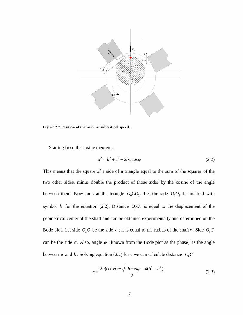
17
m
0O
2O
1F2F
nomg
1g
2g2
C
Figure 2.7 Position of the rotor at subcritical speed.
Starting from the cosine theorem:
2 2 2 2 cosa b c bc (2.2)
This means that the square of a side of a triangle equal to the sum of the squares of the
two other sides, minus double the product of those sides by the cosine of the angle
between them. Now look at the triangle 0 2O CO . Let the side 0 2O O be marked with
symbol b for the equation (2.2). Distance 0 2O O is equal to the displacement of the
geometrical center of the shaft and can be obtained experimentally and determined on the
Bode plot. Let side 2O C be the side a ; it is equal to the radius of the shaft r . Side 0O C
can be the side c . Also, angle (known from the Bode plot as the phase), is the angle
between a and b . Solving equation (2.2) for c we can calculate distance 0O C
2 22 (cos ) 2 cos 4( )
2
b b b ac
(2.3)
18
Or2 2 2
0 2 0 2 0 20
2 cos (2 cos ) 4( )
2
O O O O O O rO C
(2.4)
And, knowing the nominal air gap nomg and calculated distance 0O C we can determine
the air gap 1g which will be equal to:
1 0( )nomg g r O C (2.5)
Substituting equation (2.4) in to (2.5) one can obtain a general formula for 1g :
2 2 20 2 0 2 0 2
1
2 cos (2 cos ) 4( )( )
2nom
O O O O O O rg g r
(2.6)
Note that from equation (2.5) one can see that the air gap at the location of the center of
mass is a function of the radius of the rotor, nominal gap, displacement of the rotor, and
phase .
Now substituting 1g in to formula (2.1) in place of g one can calculate magnitude of
the force 1F that will be applied to the rotor at the point of the location of the center of
mass:
2 20
1 2 2 220 2 0 2 0 22 cos (2 cos ) 4( )
4((( ) ) )2
g
nom
A N IF
O O O O O O rg r
(2.7)
Now let’s look how the force is changing in the high beat point or response point. The
air gap 2g (see Figure 2.7) can be determined from the experimental data using formula
(2.8)
2 0 2( )nomg g r O O (2.8)
Where 0 2O O is the amplitude of the vibration, or radial displacement, of the geometrical
center of the shaft. Note that 1 2g g . But the value of the injected current will change
19
due to changing phase of the injected sinusoidal wave with the rotating of the shaft. This
phase also will be equal to the angle . So, the formula for the magnitude of the applied
force 2F at the point of response of the shaft or high beat point will be (2.9):
2 20
2 224
gA N IF
g
(2.9)
Substituting (2.8) into (2.9) the formula for calculating applied force at the high beat
point can be obtained:
2 20
2 20 24(( ) )
g
nom
A N IF
g r O O
(2.10)
As was mentioned above this force should compensate exciting force that is an
unbalance force in this case.
MatLab codes were generated for observing this force graphically. The best
performance of the rotor occurs when it rotates around its center of mass. From the
plotted graphs, we can conclude that for obtaining the force that forces the rotor rotate
around its center of mass, we need to generate a wave of current with a special shape for
injecting into magnetic actuator.
Starting with the magnetic actuator force equation:
2 20
214 cos( )
gA N IF
g t
(2.11)
It is desired to cancel the unbalance force, using the magnetic actuator force.
The equation for these forces can be stated thus:
2 202
21
cos( )4 cos( )
gA N Iml t
g t
(2.12)
20
Solving for the current gives:
2 22 1
20
cos( )4 cos( )
g
ml t g tI
A N
(2.13)
Substituting (2.6) into (2.13) gives a formula for the ideal current that needs to be
injected to cancel the unbalance exciting force:
2 2 22 20 2 0 2 0 2
2
20
2 cos (2 cos ) 4( )cos( )4( ) cos( )
2nom
g
O O O O O O rml t g r t
IA N
(2.14)
Finding the actual coil current is complicated by the switching nature of the opposing
coils in the magnetic actuator. The top coil is “on” if, and only if, the bottom coil is “off”
and vice versa. Also, the signal injection is interpreted as a negative current in a bottom
coil. Finally the switch is made dictated by the expected direction of the unbalance force
to be cancelled, as described in the formulas for all three conditions (2.15):
2 21
20
2 21
20
cos( )4 cos( )when cos( ) 0
cos( )4 cos( )when cos( ) 0
0 when cos( ) 0
g
g
ml t g tt
A N
ml t g tI t
A N
t
(2.15)
This is a complicated waveform, which is difficult to generate with conventional
hardware. It is proposed to approximate this result with a single-frequency cosine wave
because a cosine wave can be readily created using hardware common in the industry.
Starting from the constraint of a cosine form wave, three parameters must be selected to
define the injection, frequency, phase, and amplitude. To select frequency, a frequency

21
analysis of the ideal injection signal must be performed. The Figure 2.8 below is the Fast
Fourier Transform of the idealized injection signal, using parameters taken from the
experimental (which will be shown in Figure 2.10).
0 20 40 60 80 100 120 140 160 180 2000
0.05
0.1
0.15
0.2
0.25
0.3
0.35
Frequency (Hz)
Curr
ent
(A)
1X
3X
5X
Figure 2.8 Frequency response of idealized unbalance compensation injection current for rotorrunning at 1950 RPM.
It is found that the dominant frequency component is that of the running speed. This is
an intuitive result because the unbalance force, which is to be cancelled, occurs at this
frequency. The phase between the unbalance force and the rotor response is found by the
relationship between running speed and natural frequency, such that the magnetic force
will always be in the opposite direction as the unbalance force. The amplitude of current
injection is taken as the maximum amplitude of the idealized current injection.
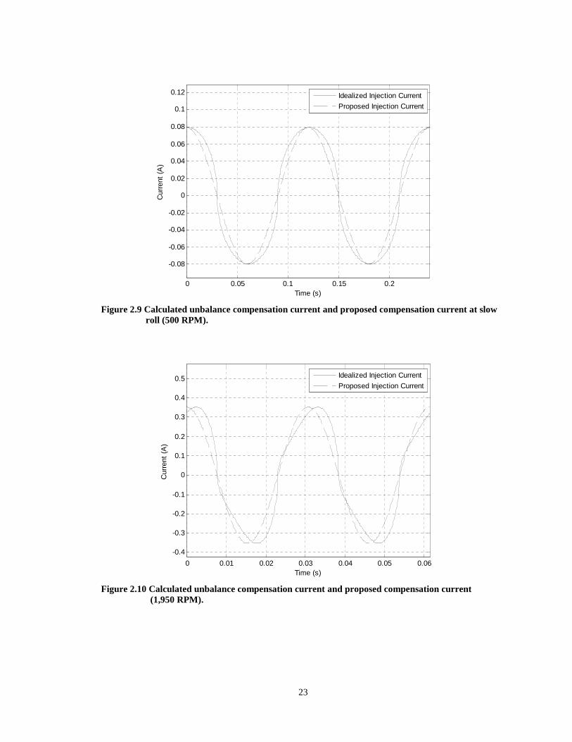
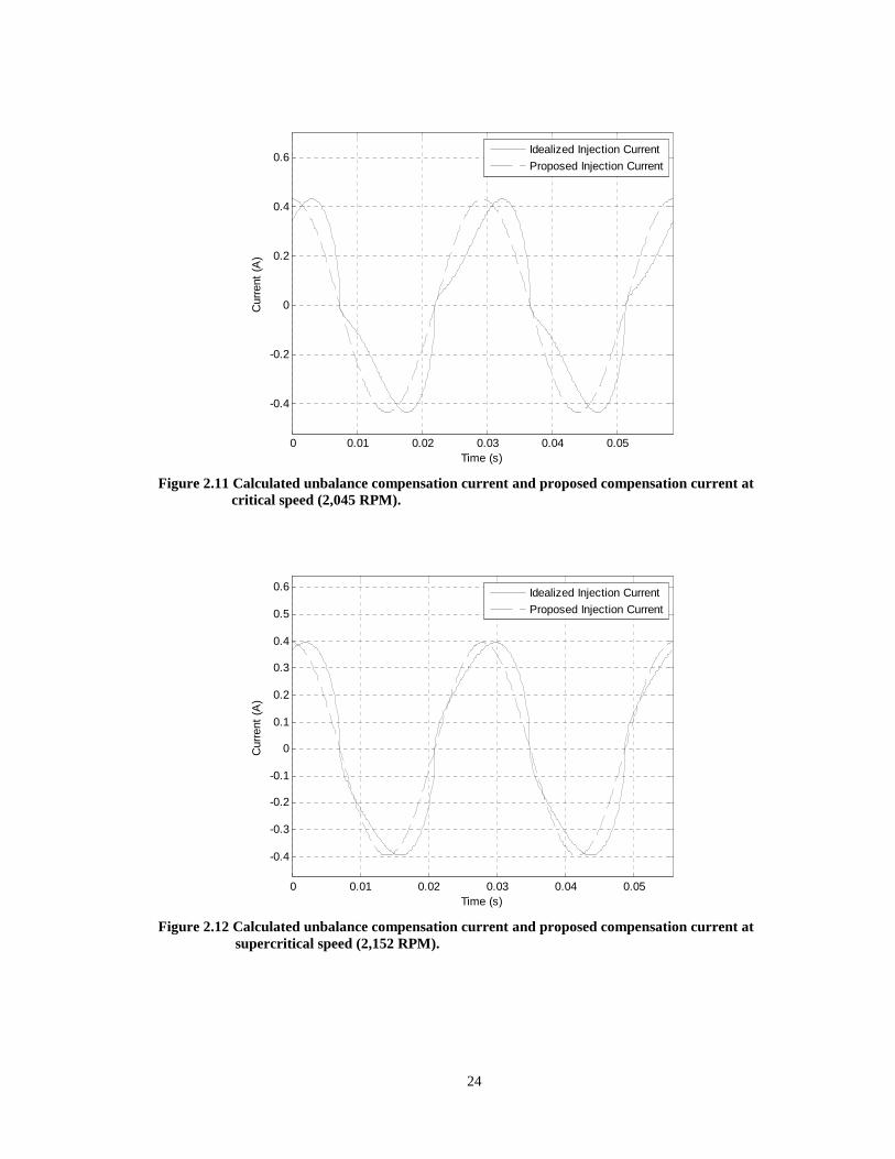
The Figures 2.9 through 2.12 shows the ideal injection current found and a
comparable cosine wave. The results for four running speeds are as follows: slow roll
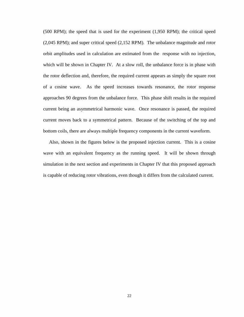
22
(500 RPM); the speed that is used for the experiment (1,950 RPM); the critical speed
(2,045 RPM); and super critical speed (2,152 RPM). The unbalance magnitude and rotor
orbit amplitudes used in calculation are estimated from the response with no injection,
which will be shown in Chapter IV. At a slow roll, the unbalance force is in phase with
the rotor deflection and, therefore, the required current appears as simply the square root
of a cosine wave. As the speed increases towards resonance, the rotor response
approaches 90 degrees from the unbalance force. This phase shift results in the required
current being an asymmetrical harmonic wave. Once resonance is passed, the required
current moves back to a symmetrical pattern. Because of the switching of the top and
bottom coils, there are always multiple frequency components in the current waveform.
Also, shown in the figures below is the proposed injection current. This is a cosine
wave with an equivalent frequency as the running speed. It will be shown through
simulation in the next section and experiments in Chapter IV that this proposed approach
is capable of reducing rotor vibrations, even though it differs from the calculated current.
23
0 0.05 0.1 0.15 0.2
-0.08
-0.06
-0.04
-0.02
0
0.02
0.04
0.06
0.08
0.1
0.12
Time (s)
Curr
ent
(A)
Idealized Injection Current
Proposed Injection Current
Figure 2.9 Calculated unbalance compensation current and proposed compensation current at slowroll (500 RPM).
0 0.01 0.02 0.03 0.04 0.05 0.06
-0.4
-0.3
-0.2
-0.1
0
0.1
0.2
0.3
0.4
0.5
Time (s)
Curr
ent
(A)
Idealized Injection Current
Proposed Injection Current
Figure 2.10 Calculated unbalance compensation current and proposed compensation current(1,950 RPM).
24
0 0.01 0.02 0.03 0.04 0.05
-0.4
-0.2
0
0.2
0.4
0.6
Time (s)
Curr
ent
(A)
Idealized Injection Current
Proposed Injection Current
Figure 2.11 Calculated unbalance compensation current and proposed compensation current atcritical speed (2,045 RPM).
0 0.01 0.02 0.03 0.04 0.05
-0.4
-0.3
-0.2
-0.1
0
0.1
0.2
0.3
0.4
0.5
0.6
Time (s)
Curr
ent
(A)
Idealized Injection Current
Proposed Injection Current
Figure 2.12 Calculated unbalance compensation current and proposed compensation current atsupercritical speed (2,152 RPM).
25
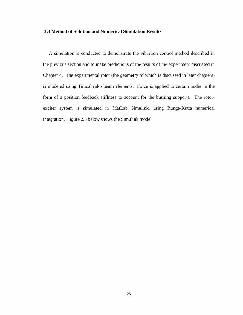
2.3 Method of Solution and Numerical Simulation Results
A simulation is conducted to demonstrate the vibration control method described in
the previous section and to make predictions of the results of the experiment discussed in
Chapter 4. The experimental rotor (the geometry of which is discussed in later chapters)
is modeled using Timoshenko beam elements. Force is applied to certain nodes in the
form of a position feedback stiffness to account for the bushing supports. The rotor-
exciter system is simulated in MatLab Simulink, using Runge-Kutta numerical
integration. Figure 2.8 below shows the Simulink model.

26
Figure 2.13 Simulink model for numerical simulation of flexible rotor with unbalance and magneticactuator compensation.
ma
gn
itu
de
of
un
ba
lan
cefo
rce
[N]
|u|2
w^2
sin
sin
sig
na
l
ge
ne
rato
r2
sig
na
l
ge
ne
rato
r1
[00
]
off
-K-
m*e
co
s
co
s
Sco
pe
1
Sco
pe
19
1
Ru
nn
ing
Sp
ee
d
x'=
Ax+
Bu
y=
Cx+
Du
Ro
tor
on
Bu
shin
gs
Pro
du
ct3
Pro
du
ct2
Pro
du
ct1
Ma
nu
al
Sw
itch
yp
osit
ion
yc
urr
en
ty
forc
e
MA
ya
xis
xp
osit
ion
xc
urr
en
tx
forc
e
MA
xa
xis
0
Clo
ck
yax
is
cu
rre
nt
[A}
xa
xis
cu
rre
nt
[A]
xa
xis
ma
gn
eti
cp
ole
po
sitio
n[u
m]
yax
ism
agn
eti
cp
ole
po
sit
ion
[um
]
xa
xis
unb
ala
nc
efo
rce
[N]
sp
ee
d
[ra
d/s
]
tim
e[s
]
on
ya
xis
un
ba
lan
ce
forc
e[N
]
xa
xis
dis
k
po
sit
ion
[um
]
ya
xis
dis
k
po
sit
ion
[um
]

27
In the simulation, the rotor running speed and eccentricity create an unbalance force
which acts only at the disk node. The unbalance force acts in vertical and horizontal
directions 90º out of phase. The magnitude of the unbalance is estimated from the orbit
of the actual rotor without vibration control as 1.68 gm-in. There is also a representation
of the magnetic actuator which may be turned “off” or turned “on” by removing or
applying its resulting force from the rotor via a manual switch block. Each axis of the
magnetic actuator is modeled using the nonlinear equation (2.15) for the top and bottom
magnetic coils in opposite directions. This is in blocks “MA x axis” and “MA y axis” for
the horizontal and vertical axis, respectively. Also, note that the rotor position is a factor
in the magnetic actuator force, which is taken from the magnetic pole node of the finite
element rotor. Figure 2.14 below shows the inside of one magnetic actuator axis block.
The saturation blocks mimic the real system, which does not accept negative current.
1
x force
-1
directionSaturation1
Saturation
f(u)
Force
Function
2 x current
1
x position
MA
f orce [N]
rotor position [um]
top coil current [A]
bot coil current [A]
Figure 2.14 Simulink model of magnetic actuator force corresponding to block “MA x axis” shown inFigure 2.8.

28
The current generators are set for sinusoidal signals with the same frequency as
rotation and out-of-phase. The current from each generator is shown in Figure 2.15
below.
50 50.01 50.02 50.03 50.04 50.05 50.06 50.07 50.08 50.09
-0.6
-0.4
-0.2
0
0.2
0.4
0.6
curr
ent
(A)
time (s)
horizontal
vertical
Figure 2.15 Sample of current signals sent to magnetic actuator in simulation.
The simulation was first run with the actuator force turned “off” and allowed to come
to steady state rotation. The position of the disk in the horizontal and vertical directions
for a characteristic span of time is shown in Figure 2.16. Note that deflection in each
direction has slightly different amplitude due to non-isotropic bearing stiffness.
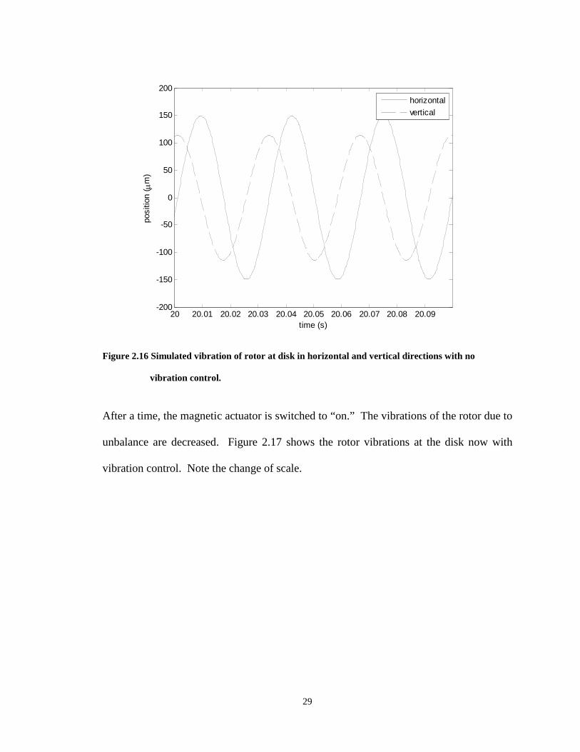
29
20 20.01 20.02 20.03 20.04 20.05 20.06 20.07 20.08 20.09-200
-150
-100
-50
0
50
100
150
200
positio
n(
m)
time (s)
horizontal
vertical
Figure 2.16 Simulated vibration of rotor at disk in horizontal and vertical directions with no
vibration control.
After a time, the magnetic actuator is switched to “on.” The vibrations of the rotor due to
unbalance are decreased. Figure 2.17 shows the rotor vibrations at the disk now with
vibration control. Note the change of scale.
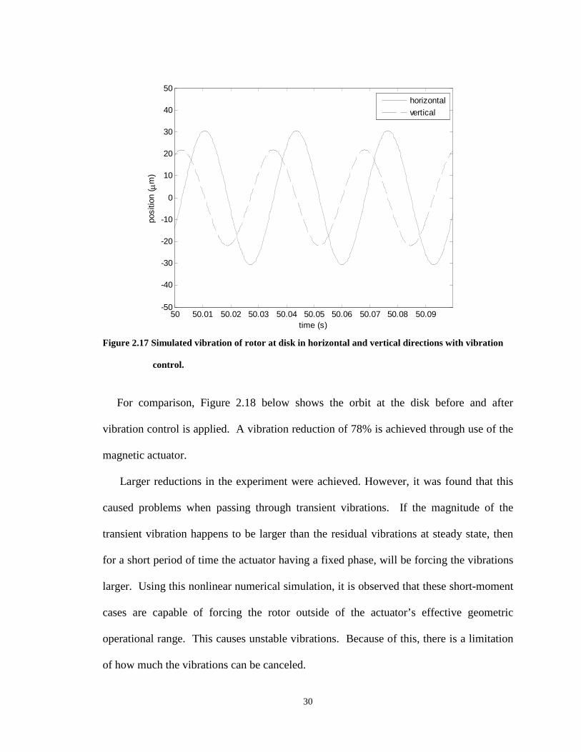
30
50 50.01 50.02 50.03 50.04 50.05 50.06 50.07 50.08 50.09-50
-40
-30
-20
-10
0
10
20
30
40
50
positio
n(
m)
time (s)
horizontal
vertical
Figure 2.17 Simulated vibration of rotor at disk in horizontal and vertical directions with vibration
control.
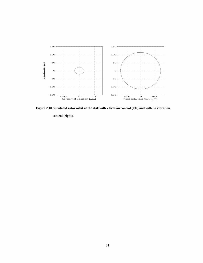
For comparison, Figure 2.18 below shows the orbit at the disk before and after
vibration control is applied. A vibration reduction of 78% is achieved through use of the
magnetic actuator.
Larger reductions in the experiment were achieved. However, it was found that this
caused problems when passing through transient vibrations. If the magnitude of the
transient vibration happens to be larger than the residual vibrations at steady state, then
for a short period of time the actuator having a fixed phase, will be forcing the vibrations
larger. Using this nonlinear numerical simulation, it is observed that these short-moment
cases are capable of forcing the rotor outside of the actuator’s effective geometric
operational range. This causes unstable vibrations. Because of this, there is a limitation
of how much the vibrations can be canceled.
31
-100 0 100-150
-100
-50
0
50
100
150
horizontal position (m)
verticalposition( m)
-100 0 100-150
-100
-50
0
50
100
150
horizontal position (m)
Figure 2.18 Simulated rotor orbit at the disk with vibration control (left) and with no vibration
control (right).

32
CHAPTER III
THE FLEXIBLE ROTOR TEST RIG
3.1 Overview of the rig
The experiment was performed using a commercial Bently Nevada Rotor Kit RK4
shown in (Figure 3.1(a)) and a modified active magnetic bearing (AMB) manufactured
by SKF Magnetic Bearings see (Figure 3.2(b)). The modified bearing serves as an
actuator. The Bently Nevada Corporation Rotor Kit is a versatile and compact example of
a rotating machine that demonstrates several patterns of shaft vibration by duplicating
vibration-producing phenomena found in large rotating machinery. This combination of
RK4 and AMB was found effective in demonstrating one of the features of active
magnetic actuators with vibration control.
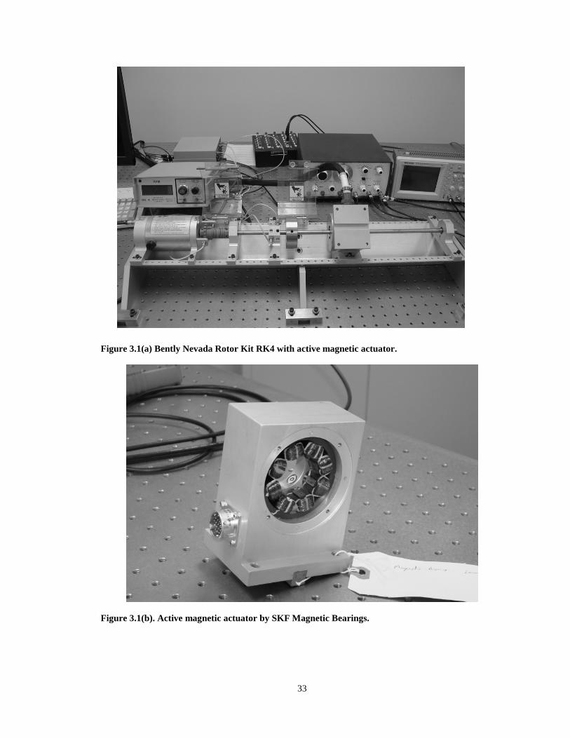
33
Figure 3.1(a) Bently Nevada Rotor Kit RK4 with active magnetic actuator.
Figure 3.1(b). Active magnetic actuator by SKF Magnetic Bearings.

34
In addition to active magnetic actuator (AMA) sensors, a Bently Nevada Rotor
Proximitor Assembly was used. Signals were transmitted first to a Bently Nevada Data
Acquisition Interface Unit (DAIU) and then to the Bently Nevada Automated Diagnostics
for Rotating Equipment software (ADRE for Windows) for displaying and recording the
data collected from the probes. The probes are located near the disk with one probe in the
vertical and one in the horizontal directions.
The stainless steel shaft is 560 mm long (22 in) and 10 mm (0.394 in) in diameter. The
weight of the rotor shaft is 350 g. One steel balance disk, 76.2 mm (3 in) in diameter,
25.4 mm (1 in) thick and weight of 0.8 kg (1.764 lb), was attached at approximately one
quarter of the rotor span from the motor side. The rotor supported by two bearings. The
radial rotor of the active magnetic actuator, which is 34.3 mm (1.35 in) in diameter, 47.8
mm (1.88 in) long and weight of 0.264 kg (0.58 lb), is placed at the bearings midspan.
The rotor was driven by an electrical motor with a separate controller. The rotor is
attached to the motor by a flexible aluminum coupling, which also incorporates speed
sensors for motor control and a Keyphasor for rotor’s angle determination.
The speed is controlled by feedback pulses from speed sensors, which observes a 20-
notch wheel mounted on the rotor coupling. The motor controller let us choose desired
rotational speed that can be selected from 250 rpm to 10,000 rpm. In addition, the speed
set point can be set to ramp up or downward at a rate of up to 15,000 rpm/min. The radial
displacement of the shaft was measured in two planes (vertical and horizontal) with eddy
current transducers or proximity probes. Proximity probes measure distances between
0.254 mm (10 mils) and 2.28 mm (90 mils). The proximity probes signal is generated by
measuring voltage changes in the proximity probes circuit. The Keyphasor let us know
35
the angular location (phase) of the shaft vibration response in relation to the physical
location of the event (Figure 3.2). Also, we used a keyphasor for triggering a Wavetek
5MHz LIN/LOG sweep generator that produced an injected sine wave, to be described
later in this chapter.
V
0
One)360(Re 0volution
probe
proximity
Figure 3.2 Keyphasor sensor used to determine the phase.
3.2 Redesign of active magnetic actuator
An active magnetic actuator (AMA) was used for vibration control, its specification
presented in Appendix C.
The AMA system consists of a stator, a rotor with an internal collet, position sensors,
touchdown bearing, a control system and power amplifiers. The rotor, which is made of
laminated iron, is attached the shaft with the collet. The magnetic actuators and sensors
are located on opposite sides of the rotor in two perpendicular control axes. The control
system and amplifiers are located in a separate housing and connected by wires. The
stator is also made of laminated steel with poles on the internal diameter. Wire coils are
wound around each pole, so that the actuator is divided into four quadrants, each having
two poles. In our case, quadrants are aligned strictly vertically and horizontally.
36
Opposing quadrants constitute an axis and, therefore, each actuator can be described by
two perpendicular axes. So each actuator’s axis has a pair of amplifiers to provide current
to generate an attractive magnetic force to correct the position of the rotor along that
particular axis. The amplifiers, which are of pulse with modulation (PWM) type, are high
voltage switches that are turned “on” and “off” at a high frequency, to achieve a current
in the coils requested by the controller. The stator and rotor are the active bearing
elements used to apply force to the shaft. The application of magnetic actuators is based
upon the principle that an electromagnet will attract ferromagnetic material. The sensor
ring measures radial position of the shaft and is mounted as close to the actuator as
possible. The sensors feed information about the position of the shaft to the controller in
the form of an electrical voltage. The touchdown bearing is not in contact with the rotor
during normal operation and used to protect the magnetic poles when vibration of the
shaft exceeds admissible level. See Figure3.3, which shows the components
disassembled. The touchdown bearing used on this are deep groove ball bearings
mounted in the actuator housing. The clearance between the shaft and the touchdown
bearing is approximately half of that between the magnetic bearing rotor and stator. The
original magnetic bearing was designed for 3/8 inch diameter shaft. Bently Nevada’s
Rotor Kit RK4 uses a shaft 10mm in diameter. To keep the same clearance between the
shaft and the touchdown bearing, a new bearing ring with necessary dimensions was
produced.

37
Figure 3.3 Components of the active magnetic actuator.
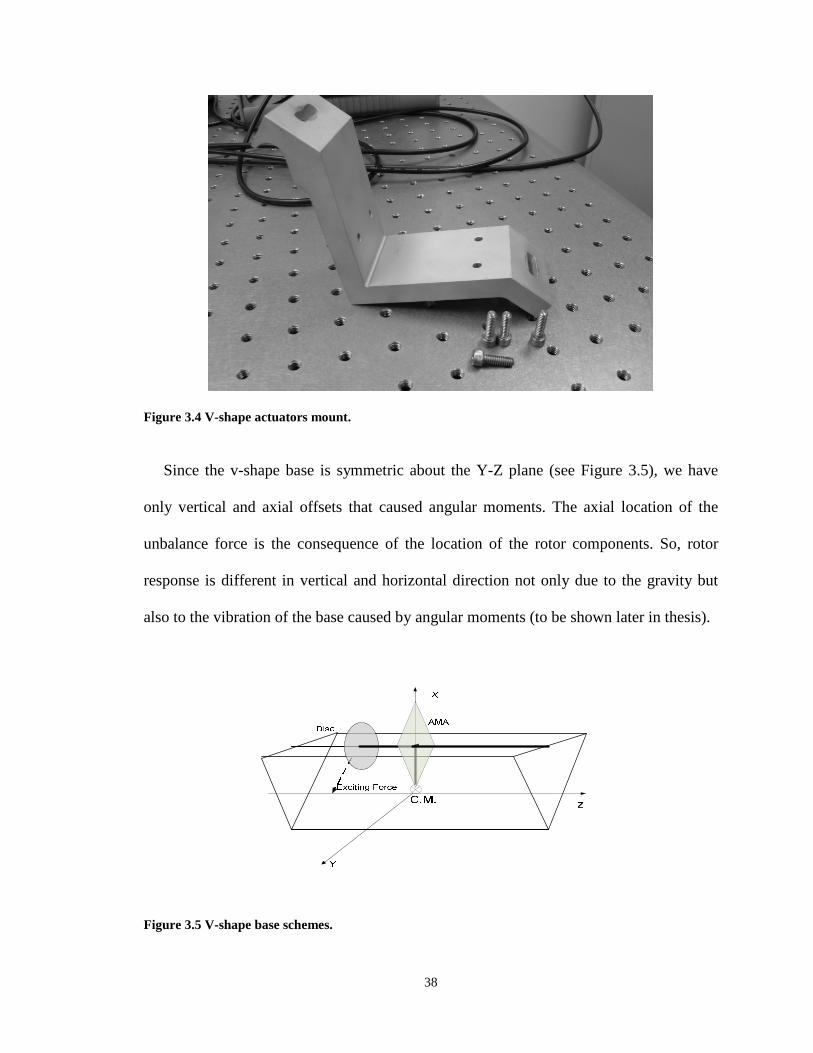
As was mentioned above, a V-shape base from Bently Nevada was used. A special V-
shape mount was designed and manufactured for mounting the active magnetic actuator
by Revolve Magnetic Bearings, Inc. The V-shape mount is shown in Figure 3.4. Since the
V-shape rotor kit’s base is being perturbed by an unbalance force in the X-Y plane, there
always is a harmonic force applied in the vertical and horizontal directions, no matter
where the perturbation plane is. But it is possible to reduce the torque on the base by
reducing the length of the moment arm between the perturbation force (unbalance at the
disk) and the center of mass of the base.
TouchdownBearing withadjusting ring
RadialRotor
TaperedSleeve
Housing withRadial Statorand RadialSensor
38
Figure 3.4 V-shape actuators mount.
Since the v-shape base is symmetric about the Y-Z plane (see Figure 3.5), we have
only vertical and axial offsets that caused angular moments. The axial location of the
unbalance force is the consequence of the location of the rotor components. So, rotor
response is different in vertical and horizontal direction not only due to the gravity but
also to the vibration of the base caused by angular moments (to be shown later in thesis).
Figure 3.5 V-shape base schemes.

39
To minimize these moments as much as possible, the mount was designed to keep the
center of mass of the rig as close to the axis of rotation as possible. See Figure 3.6.
Figure 3.6 Active magnetic actuator assembled on a V-shape base.
The active magnetic actuator was connected to the MB350 Controller. See Figure 3.7.
The MB350 Controller is a self-contained, fully digital, magnetic bearing control system.
It has a great number of features. But, to make this method of reducing vibration more
attractive and easy to use, only a simple one is used. The function of the controller is to
receive and process the voltage signal from the position sensors and inject and calculate a
feedback control current. Here it is used for accepting and sending externally-generated
harmonic current to the active magnetic actuator. The MB350 controller was connected
to the computer via MBScope software. MBScope is a Windows-based software program
designed to provide full access to the functional capabilities of SKF magnetic bearing
controllers. System parameters such as position and current can be monitored with an
external computer connected with a parallel cable. The software provides a rich,
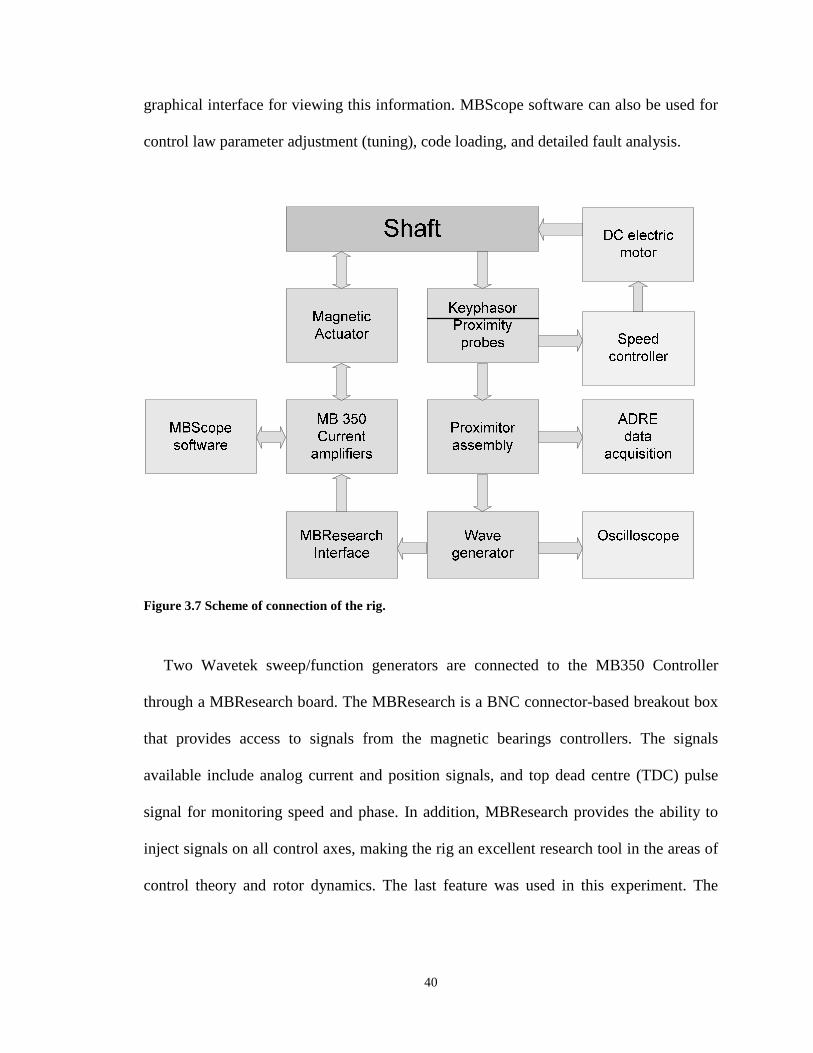
40
graphical interface for viewing this information. MBScope software can also be used for
control law parameter adjustment (tuning), code loading, and detailed fault analysis.
Figure 3.7 Scheme of connection of the rig.
Two Wavetek sweep/function generators are connected to the MB350 Controller
through a MBResearch board. The MBResearch is a BNC connector-based breakout box
that provides access to signals from the magnetic bearings controllers. The signals
available include analog current and position signals, and top dead centre (TDC) pulse
signal for monitoring speed and phase. In addition, MBResearch provides the ability to
inject signals on all control axes, making the rig an excellent research tool in the areas of
control theory and rotor dynamics. The last feature was used in this experiment. The

41
MBResearch board connects to the magnetic actuator controller via 68-pin SCSI
connector.
Two Wavetek sweep/function generators are taken for generating and injecting sine
waves in the vertical and horizontal directions. Model 185 and model FG3B are used in
this experiment. Wavetek generators are a precision source of sine, triangle square,
positive pulse and negative pulse waveforms as well as a DC voltage supply. The
frequency of the waveforms is manually or remotely variable from 100 Hz to 5 Hz .
Frequencies can be swept both linearly and logarithmically. The amplitude of the
waveforms is variable from 20V p-p, open circuit maximum, to -80dB. The waveforms
can be given a DC offset positively and negatively. The symmetry of the waveforms is
continuously adjustable from approximately 1:19 to 19:1. Varying symmetry provides
variable duty cycle pulses, sawtooth and asymmetrical sine waveforms. The heart of the
generator consists of the positive and negative current sources, the current switch, timing
capacitors, triangle amplifier, and hysteresis switch. The positive and negative current
sources generate equal but opposite polarity currents, which charge and discharge the
timing capacitor selected by the range selector. The current switch, which is controlled by
the hysteresis switch, selects either the positive or negative current as the input to the
capacitor. Since the capacitor is being charged by a current source, which changes
polarity periodically, the voltage across the capacitor forms a triangle waveform and
reaches predetermined positive and negative peak values. When this occurs, the output of
the hysteresis changes state and causes the current switch to select the opposite polarity
current. The output of the hysteresis switch is a square wave whose edges correspond to
the triangle peak values. The magnitude of the current produced by the current sources is
42
dependent upon the output of the voltage controlled generator (VCG) amplifier. By
varying the output of the VCG amplifier, the frequency of the triangle and square
waveforms may be controlled. In order to generate sine waves, the triangle waveform is
sine shaped in the sine converter circuit with nonlinear elements. The waveforms switch
selects the waveform of interest and the portion of the signal is selected by the amplitude
potentiometer and applied to the output amplifier. The output amplifier is capable of
driving a 50 load and may be DC offset. The amplifier output is routed to a 50
attenuator which can provide 60dB of attenuation in 20dB steps. An additional 20dB of
attenuation can be obtained from the amplitude control. We used the generator in the
trigger mode. In the trigger mode, the generator is stopped by the amplifier. This
amplifier compares the output of the triangle amplifier to ground. Its output draws just
the right amount of current away from the capacitor to keep it at zero volts. This level is
known as the “trigger baseline”. When the external signal is applied to the trigger input, it
is shaped into a fast rise time pulse by squaring the circuit and is applied to the trigger
logic circuit. This circuit in turn shuts off the trigger amplifier for one cycle of the output
waveform [22].
The wave generators are triggered by the signal received from the Bently Nevada
Rotor Kit Proximitor Assembly. That signal is taken from the Keyphasor probe. Also this
signal was sent to the interface and then to an independent data acquisition system.
An Automated Diagnostics for Rotating Equipment (ADRE) system was used. The
ADRE system is specifically designed for real-time highly parallel signal processing and
presentation. This system incorporates the functionality of many types of instrumentation,
such as oscilloscopes, spectrum analyzers, filters, signal conditioners, and digital

43
recorders into a single platform. The system’s real-time display capability permits it to
continuously display data independently of data being stored to permanent memory. An
ADRE data acquisition system consists of a Bently Nevada 408 Dynamic Signal
Processing Instrument, ADRE client software, and a computer capable of running ADRE
software. The Bently Nevada data acquisition interface unit (DAIU) 408 supports many
standard and non-standard input types, including both dynamic transducer signals (such
as those from proximity probes), and static transducer signals (such as process variables
from transmitters and distributed control systems). For rotating machinery, a Keyphasor
or other speed input signal can be used. A Keyphasor with a 1 TDC mark is used for
phase and a speed sensor with a 28 teeth is used for speed.
Also, we used a Tektronix TDS210 oscilloscope for observation and synchronization.
The Tektronix TDS210 oscilloscope is a graph-displaying device. It draws a graphical
representation a voltage signal. In most applications, the graph shows how signals change
over time: The vertical axis represents voltage and the horizontal axis represents time. A
third axis is indicated by the intensity or brightness of the display.
The Tektronix TDS210 oscilloscope's simple graph can tell many things about a
signal such as:
The time and voltage values of a signal.
The frequency of an oscillating signal.
The “moving parts” of a circuit represented by the signal.
The frequency with which a particular portion of the signal is occurring relative
to, other portions.
44
Whether or not a malfunctioning component is distorting the signal
How much of a signal is direct current (DC) or alternating current (AC) and how
much of the signal is noise.
Whether the noise is changing with time.
The specification for the Tektronix TDS 210 oscilloscope is presented in Table 3.3.
3.3 Rotordynamic modeling
Mathematical modeling is done in order to estimate the parameters of the mechanical
system such as unbalance and to validate the assumptions made in Chapter II. Finite
element analysis is applied in modeling of the rotor-bearing system using the finite
element modeling software. A Campbell diagram is drawn and the calculation of critical
speeds and mode shapes for the rotor on journal bearings (and with active magnetic
actuator off) are made. A determination of the magnitude of the unbalance is made by
assuming static unbalance at the disk and tuning orbit to experimental data. Also included
are the prediction of static deflection of the rotor and the critical speed map.
The finite element model consists of 53 Timoshenko beam elements with eight
degrees of freedom each and takes into account rotational inertia and shear deformation.
The model is shown in Figure 3.8.
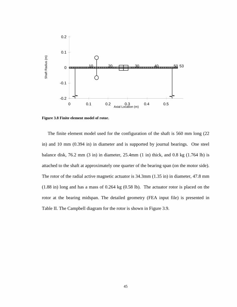
45
535040302010
-0.2
-0.1
0
0.1
0.2
0 0.1 0.2 0.3 0.4 0.5Axial Location (m)
Shaft
Radiu
s(m
)
Figure 3.8 Finite element model of rotor.
The finite element model used for the configuration of the shaft is 560 mm long (22
in) and 10 mm (0.394 in) in diameter and is supported by journal bearings. One steel
balance disk, 76.2 mm (3 in) in diameter, 25.4mm (1 in) thick, and 0.8 kg (1.764 lb) is
attached to the shaft at approximately one quarter of the bearing span (on the motor side).
The rotor of the radial active magnetic actuator is 34.3mm (1.35 in) in diameter, 47.8 mm
(1.88 in) long and has a mass of 0.264 kg (0.58 lb). The actuator rotor is placed on the
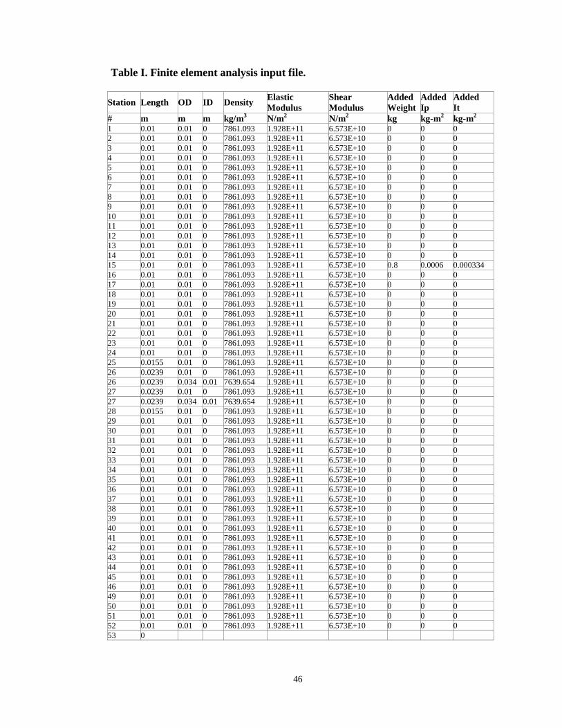
rotor at the bearing midspan. The detailed geometry (FEA input file) is presented in
Table II. The Campbell diagram for the rotor is shown in Figure 3.9.
46
Table I. Finite element analysis input file.
Station Length OD ID DensityElasticModulus
ShearModulus
AddedWeight
AddedIp
AddedIt
# m m m kg/m3 N/m2 N/m2 kg kg-m2 kg-m2
1 0.01 0.01 0 7861.093 1.928E+11 6.573E+10 0 0 02 0.01 0.01 0 7861.093 1.928E+11 6.573E+10 0 0 03 0.01 0.01 0 7861.093 1.928E+11 6.573E+10 0 0 04 0.01 0.01 0 7861.093 1.928E+11 6.573E+10 0 0 05 0.01 0.01 0 7861.093 1.928E+11 6.573E+10 0 0 06 0.01 0.01 0 7861.093 1.928E+11 6.573E+10 0 0 07 0.01 0.01 0 7861.093 1.928E+11 6.573E+10 0 0 08 0.01 0.01 0 7861.093 1.928E+11 6.573E+10 0 0 09 0.01 0.01 0 7861.093 1.928E+11 6.573E+10 0 0 010 0.01 0.01 0 7861.093 1.928E+11 6.573E+10 0 0 011 0.01 0.01 0 7861.093 1.928E+11 6.573E+10 0 0 012 0.01 0.01 0 7861.093 1.928E+11 6.573E+10 0 0 013 0.01 0.01 0 7861.093 1.928E+11 6.573E+10 0 0 014 0.01 0.01 0 7861.093 1.928E+11 6.573E+10 0 0 015 0.01 0.01 0 7861.093 1.928E+11 6.573E+10 0.8 0.0006 0.00033416 0.01 0.01 0 7861.093 1.928E+11 6.573E+10 0 0 017 0.01 0.01 0 7861.093 1.928E+11 6.573E+10 0 0 018 0.01 0.01 0 7861.093 1.928E+11 6.573E+10 0 0 019 0.01 0.01 0 7861.093 1.928E+11 6.573E+10 0 0 020 0.01 0.01 0 7861.093 1.928E+11 6.573E+10 0 0 021 0.01 0.01 0 7861.093 1.928E+11 6.573E+10 0 0 022 0.01 0.01 0 7861.093 1.928E+11 6.573E+10 0 0 023 0.01 0.01 0 7861.093 1.928E+11 6.573E+10 0 0 024 0.01 0.01 0 7861.093 1.928E+11 6.573E+10 0 0 025 0.0155 0.01 0 7861.093 1.928E+11 6.573E+10 0 0 026 0.0239 0.01 0 7861.093 1.928E+11 6.573E+10 0 0 026 0.0239 0.034 0.01 7639.654 1.928E+11 6.573E+10 0 0 027 0.0239 0.01 0 7861.093 1.928E+11 6.573E+10 0 0 027 0.0239 0.034 0.01 7639.654 1.928E+11 6.573E+10 0 0 028 0.0155 0.01 0 7861.093 1.928E+11 6.573E+10 0 0 029 0.01 0.01 0 7861.093 1.928E+11 6.573E+10 0 0 030 0.01 0.01 0 7861.093 1.928E+11 6.573E+10 0 0 031 0.01 0.01 0 7861.093 1.928E+11 6.573E+10 0 0 032 0.01 0.01 0 7861.093 1.928E+11 6.573E+10 0 0 033 0.01 0.01 0 7861.093 1.928E+11 6.573E+10 0 0 034 0.01 0.01 0 7861.093 1.928E+11 6.573E+10 0 0 035 0.01 0.01 0 7861.093 1.928E+11 6.573E+10 0 0 036 0.01 0.01 0 7861.093 1.928E+11 6.573E+10 0 0 037 0.01 0.01 0 7861.093 1.928E+11 6.573E+10 0 0 038 0.01 0.01 0 7861.093 1.928E+11 6.573E+10 0 0 039 0.01 0.01 0 7861.093 1.928E+11 6.573E+10 0 0 040 0.01 0.01 0 7861.093 1.928E+11 6.573E+10 0 0 041 0.01 0.01 0 7861.093 1.928E+11 6.573E+10 0 0 042 0.01 0.01 0 7861.093 1.928E+11 6.573E+10 0 0 043 0.01 0.01 0 7861.093 1.928E+11 6.573E+10 0 0 044 0.01 0.01 0 7861.093 1.928E+11 6.573E+10 0 0 045 0.01 0.01 0 7861.093 1.928E+11 6.573E+10 0 0 046 0.01 0.01 0 7861.093 1.928E+11 6.573E+10 0 0 049 0.01 0.01 0 7861.093 1.928E+11 6.573E+10 0 0 050 0.01 0.01 0 7861.093 1.928E+11 6.573E+10 0 0 051 0.01 0.01 0 7861.093 1.928E+11 6.573E+10 0 0 052 0.01 0.01 0 7861.093 1.928E+11 6.573E+10 0 0 053 0
47
-150
-100
-50
0
50
100
150
200
0 2000 4000 6000 8000 10000
Rotor Speed (rpm)
Natu
ralF
req
uency
(Hz)
.
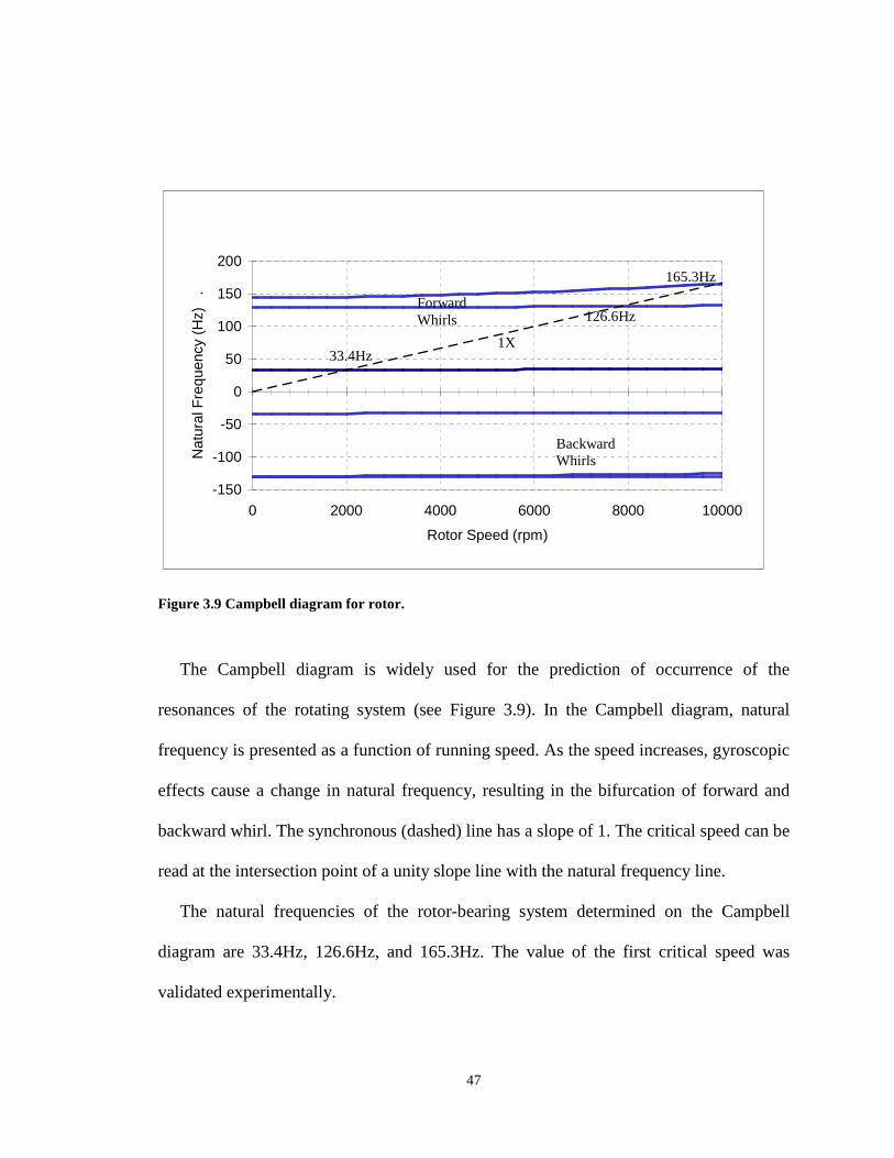
Figure 3.9 Campbell diagram for rotor.
The Campbell diagram is widely used for the prediction of occurrence of the
resonances of the rotating system (see Figure 3.9). In the Campbell diagram, natural
frequency is presented as a function of running speed. As the speed increases, gyroscopic
effects cause a change in natural frequency, resulting in the bifurcation of forward and
backward whirl. The synchronous (dashed) line has a slope of 1. The critical speed can be
read at the intersection point of a unity slope line with the natural frequency line.
The natural frequencies of the rotor-bearing system determined on the Campbell
diagram are 33.4Hz, 126.6Hz, and 165.3Hz. The value of the first critical speed was
validated experimentally.
ForwardWhirls
BackwardWhirls
1X33.4Hz
126.6Hz
165.3Hz
48
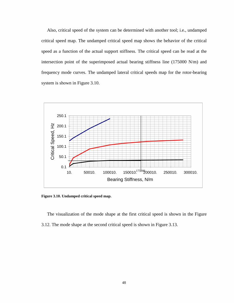
Also, critical speed of the system can be determined with another tool; i.e., undamped
critical speed map. The undamped critical speed map shows the behavior of the critical
speed as a function of the actual support stiffness. The critical speed can be read at the
intersection point of the superimposed actual bearing stiffness line (175000 N/m) and
frequency mode curves. The undamped lateral critical speeds map for the rotor-bearing
system is shown in Figure 3.10.
0.1
50.1
100.1
150.1
200.1
250.1
10. 50010. 100010. 150010. 200010. 250010. 300010.
Bearing Stiffness, N/m
Critic
alS
pe
ed
,H
z
Figure 3.10. Undamped critical speed map.
The visualization of the mode shape at the first critical speed is shown in the Figure
3.12. The mode shape at the second critical speed is shown in Figure 3.13.
175000
49
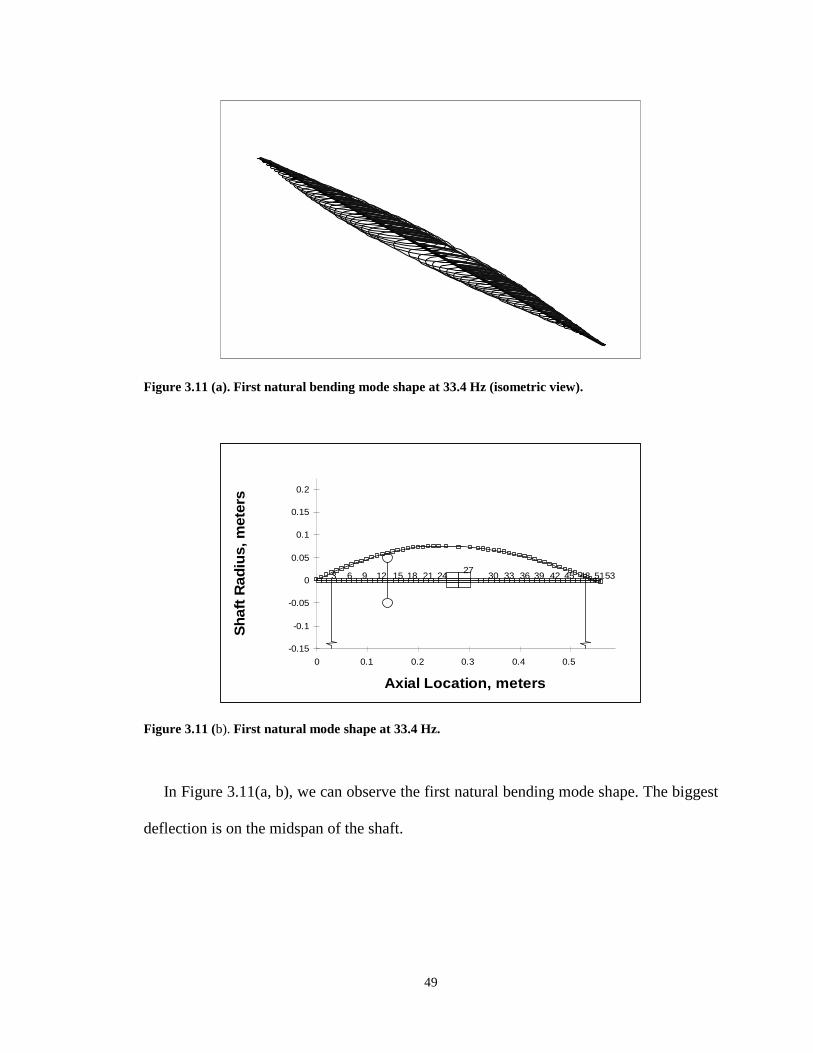
Figure 3.11 (a). First natural bending mode shape at 33.4 Hz (isometric view).
53514845423936333027
2421181512963
-0.15
-0.1
-0.05
0
0.05
0.1
0.15
0.2
0 0.1 0.2 0.3 0.4 0.5
Axial Location, meters
Sh
aft
Rad
ius,m
ete
rs
Figure 3.11 (b). First natural mode shape at 33.4 Hz.
In Figure 3.11(a, b), we can observe the first natural bending mode shape. The biggest
deflection is on the midspan of the shaft.
50
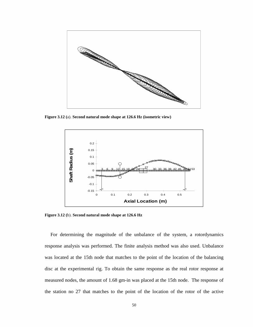
Figure 3.12 (a). Second natural mode shape at 126.6 Hz (isometric view)
53514845423936333027
2421181512963
-0.15
-0.1
-0.05
0
0.05
0.1
0.15
0.2
0 0.1 0.2 0.3 0.4 0.5
Axial Location (m)
Shaft
Radiu
s(m
)
Figure 3.12 (b). Second natural mode shape at 126.6 Hz
For determining the magnitude of the unbalance of the system, a rotordynamics
response analysis was performed. The finite analysis method was also used. Unbalance
was located at the 15th node that matches to the point of the location of the balancing
disc at the experimental rig. To obtain the same response as the real rotor response at
measured nodes, the amount of 1.68 gm-in was placed at the 15th node. The response of
the station no 27 that matches to the point of the location of the rotor of the active

51
magnetic actuator is shown in Figure 3.13. The response of the modeled node at the real
rig was measured by the active magnetic actuator sensors and will be shown in Chapter
IV.
0
0.1
0.2
0.3
0.4
0.5
0.6
0 2000 4000 6000 8000 10000 12000
Rotor Speed (rpm)
Re
sp
on
se
(mm
p-p
)
Horz Amp
Vert Amp
Figure 3.13. Simulated rotordynamics response plot at the location of the rotor of the active
magnetic actuator.
The response of the 11th and 12th stations that matches the points of the location of
the proximity probes is shown in Figures 3.14 and 3.15.
52
0
0.05
0.1
0.15
0.2
0.25
0.3
0 2000 4000 6000 8000 10000 12000
Rotor Speed (rpm)
Res
po
nse
(mm
p-p
)
-720
-630
-540
-450
-360
-270
-180
-90
0
90
180
270
360
Horz Amp
Horz Phs
Figure 3.14. Simulated rotordynamic response plot at the location of the ADRE horizontal
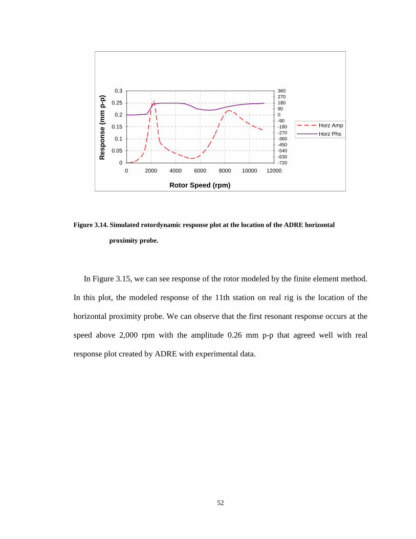
proximity probe.
In Figure 3.15, we can see response of the rotor modeled by the finite element method.
In this plot, the modeled response of the 11th station on real rig is the location of the
horizontal proximity probe. We can observe that the first resonant response occurs at the
speed above 2,000 rpm with the amplitude 0.26 mm p-p that agreed well with real
response plot created by ADRE with experimental data.
53
0
0.05
0.1
0.15
0.2
0.25
0.3
0.35
0 2000 4000 6000 8000 10000 12000
Rotor Speed, rpm
Re
sp
on
se
,m
mp
-p
-720-630
-540-450
-360-270
-180-90
090
180270
360
Vert Amp
Vert Phs
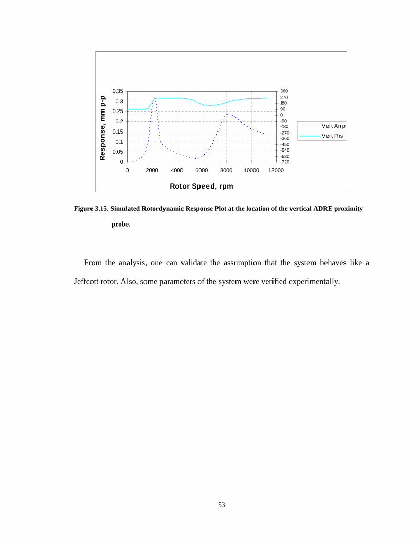
Figure 3.15. Simulated Rotordynamic Response Plot at the location of the vertical ADRE proximity
probe.
From the analysis, one can validate the assumption that the system behaves like a
Jeffcott rotor. Also, some parameters of the system were verified experimentally.

54
CHAPTER IV
UNBALANCE COMPENSATION EXPERIMENTAL RESULTS
4.1. Introduction
As previously stated an experiment was conducted on the rig with the following
configuration. The shaft is 560 mm long (22 in), 10 mm (0.394 in) in diameter and
supported by journal bearings. The active magnetic actuator is installed at the midspan of
the shaft and one steel balance disk, 76.2 mm (3in) in diameter, 25.4 mm (1in) thick and
0.8kg (1.764lb) is attached at approximately one quarter of the shaft’s span from the
coupling. Two Wavetek sweep/function generators are used for generating and injecting
sine wave current in the vertical and horizontal axis of the active magnetic actuator. The
function generators are triggered with a once per revolution keyphasor. To determine the
model identification, an impact hammer test was carried out. Two types of results are
55
presented in this work: one for constant subcritical speed and the second for speed range
crossing the resonant first natural frequency.
4.2. Experimental Results.
4.2.1. System Identification.
The model validation of the experimental rig was performed for the configuration
described above with the active magnetic actuator turned “off” (no injection). The
transfer function of the rotor was measured using impact hammer modal testing. The
measurements were carried out on the non-rotating rotor in the vertical plane. The
calibrated impulse hammer excited the rotor at the non-drive end. The response of the
rotor was measured with an accelerometer, fixed on the rotor. The input and output were
analyzed using the Hewlett Packard 35670A dynamic signal analyzer shown in
Figure 4.1.
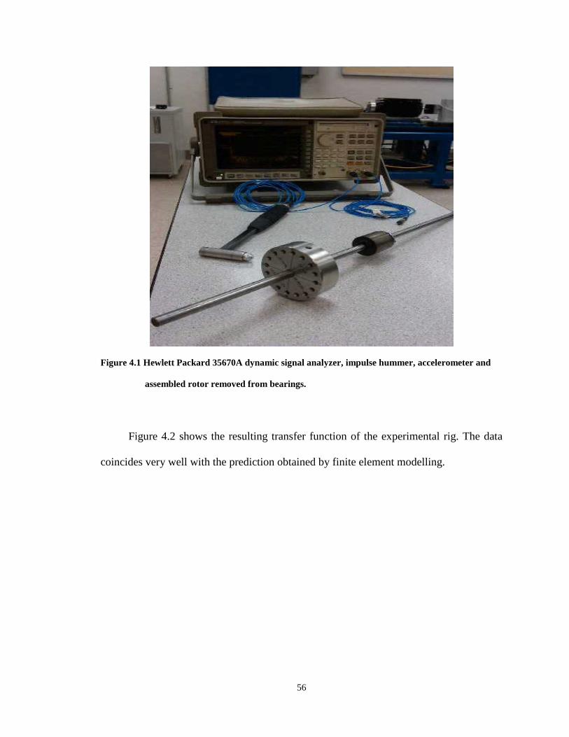
56
Figure 4.1 Hewlett Packard 35670A dynamic signal analyzer, impulse hummer, accelerometer and
assembled rotor removed from bearings.
Figure 4.2 shows the resulting transfer function of the experimental rig. The data
coincides very well with the prediction obtained by finite element modelling.
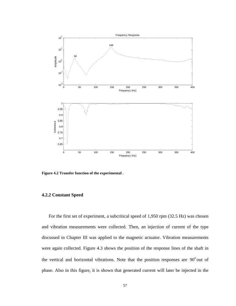
57
0 50 100 150 200 250 300 350 40010
-2
10-1
100
101
102
Frequency Response
Am
plit
ude
Frequency (Hz)
0 50 100 150 200 250 300 350 400
0.65
0.7
0.75
0.8
0.85
0.9
0.95
1
Cohere
nce
Frequency (Hz)
34
148
Figure 4.2 Transfer function of the experimental .
4.2.2 Constant Speed
For the first set of experiment, a subcritical speed of 1,950 rpm (32.5 Hz) was chosen
and vibration measurements were collected. Then, an injection of current of the type
discussed in Chapter III was applied to the magnetic actuator. Vibration measurements
were again collected. Figure 4.3 shows the position of the response lines of the shaft in
the vertical and horizontal vibrations. Note that the position responses are 090 out of
phase. Also in this figure, it is shown that generated current will later be injected in the

58
vertical and horizontal direction to decrease the position response amplitudes.
Amplitudes of the vertical and horizontal injections are 0.69 A and 0.66 A, respectively.
The frequency is the same for all of the lines and corresponds to the rotating speed of
1,950 rpm (32.5 Hz).
Figure 4.3. Uncompensated response of the shaft at magnetic actuator sensor and required current.
In Figures 4.3 through 4.7, the V13 and W13 positions represent the response of the
shaft in the vertical and horizontal planes respectively. The V13 Post Inject and W13 Post
Inject represent the current injected into the active magnetic actuator’s poles in the
vertical and horizontal axes, respectively.
VerticalResponse
HorizontalResponse
HorizontalInjection
VerticalInjection
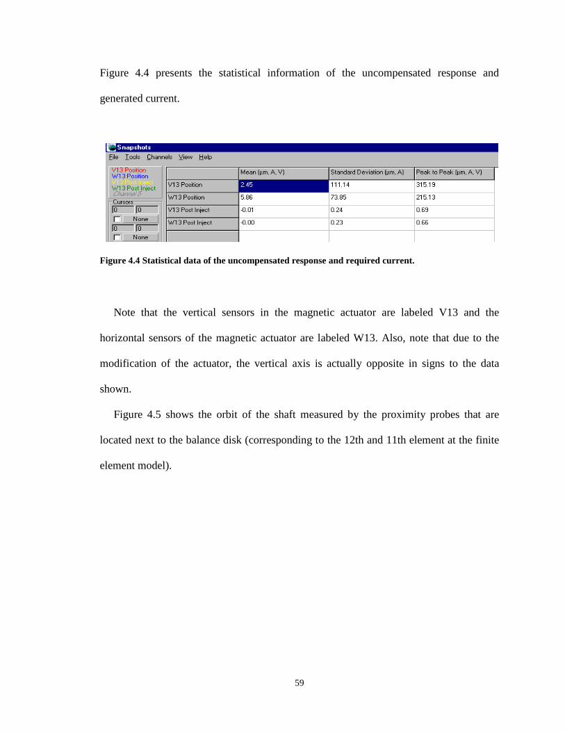
59
Figure 4.4 presents the statistical information of the uncompensated response and
generated current.
Figure 4.4 Statistical data of the uncompensated response and required current.
Note that the vertical sensors in the magnetic actuator are labeled V13 and the
horizontal sensors of the magnetic actuator are labeled W13. Also, note that due to the
modification of the actuator, the vertical axis is actually opposite in signs to the data
shown.
Figure 4.5 shows the orbit of the shaft measured by the proximity probes that are
located next to the balance disk (corresponding to the 12th and 11th element at the finite
element model).
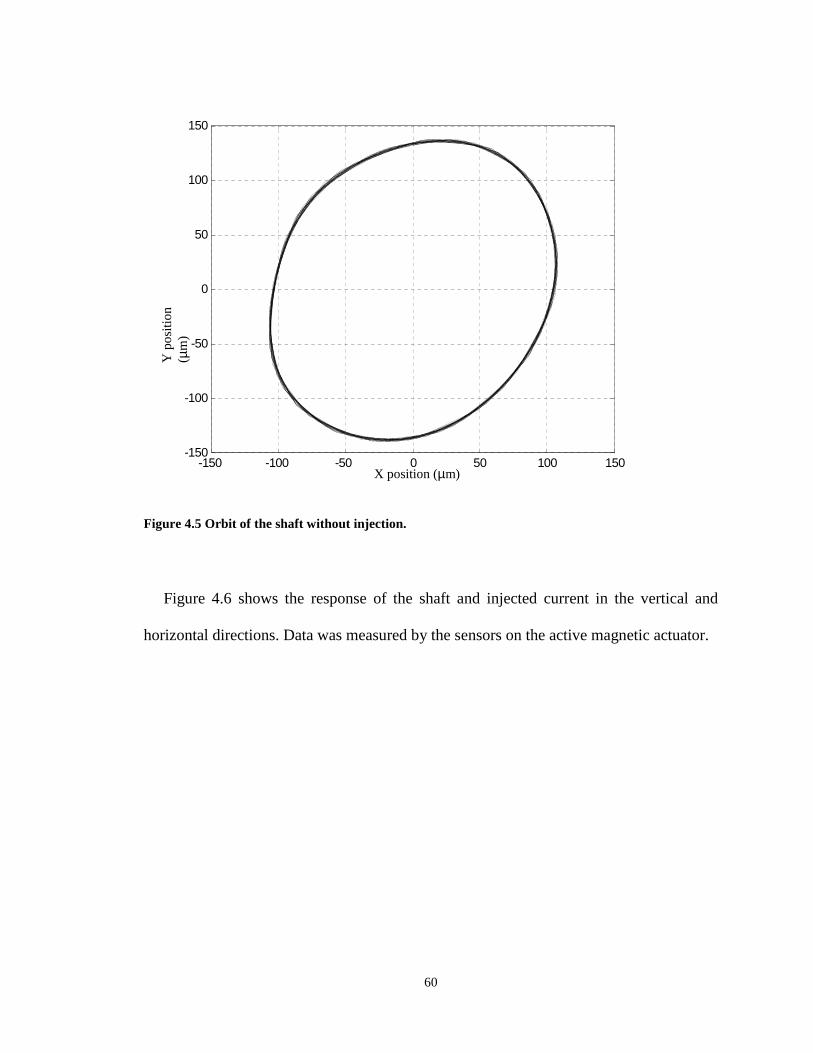
60
Figure 4.5 Orbit of the shaft without injection.
Figure 4.6 shows the response of the shaft and injected current in the vertical and
horizontal directions. Data was measured by the sensors on the active magnetic actuator.
-150 -100 -50 0 50 100 150-150
-100
-50
0
50
100
150
Yp
osi
tio
n(µ
m)
X position (µm)
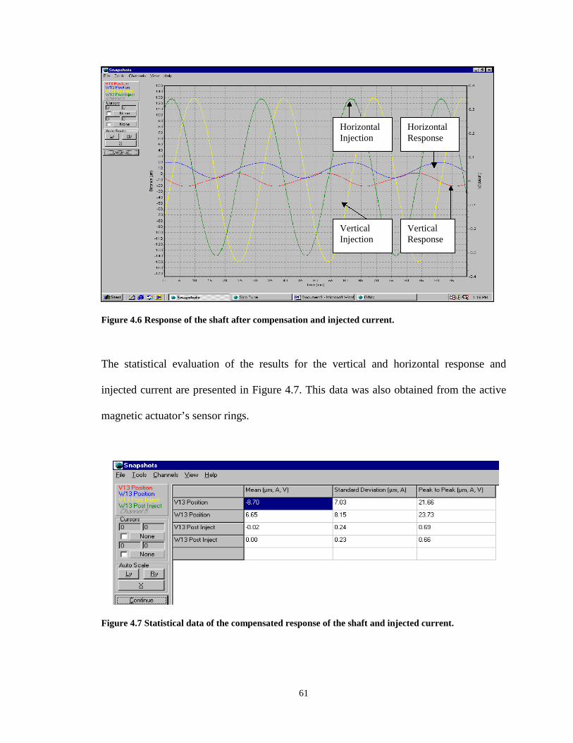
61
Figure 4.6 Response of the shaft after compensation and injected current.
The statistical evaluation of the results for the vertical and horizontal response and
injected current are presented in Figure 4.7. This data was also obtained from the active
magnetic actuator’s sensor rings.
Figure 4.7 Statistical data of the compensated response of the shaft and injected current.
VerticalResponse
VerticalInjection
HorizontalResponse
HorizontalInjection

62
The response of the rotor was also measured by the ADRE proximity probes. ADRE
data, presented in Figure 4.8, shows the orbit of the shaft measured at the position next to
the balance disk, after the force was applied to the shaft by the magnetic actuator.
Figure 4.8 Orbit of the shaft with injection.
In Figures 4.6 through 4.8, a significant reduction in the vibration amplitude of the
shaft is observed. Figure 4.9 compares the vibration amplitude both with and without
current injection on the same scale. A reduction of amplitude of over 90% was achieved.
-15 -10 -5 0 5 10 15-10
-8
-6
-4
-2
0
2
4
6
8
10
Yp
osi
tio
n(µ
m)
X position (µm)
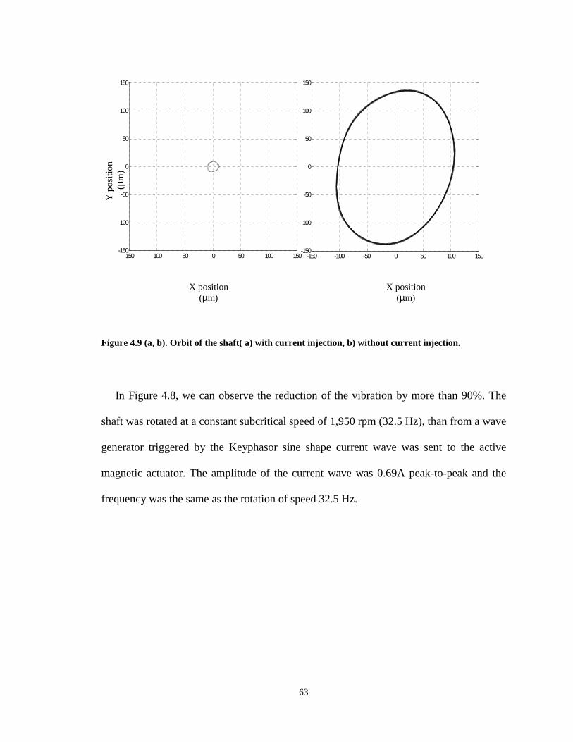
63
Figure 4.9 (a, b). Orbit of the shaft( a) with current injection, b) without current injection.
In Figure 4.8, we can observe the reduction of the vibration by more than 90%. The
shaft was rotated at a constant subcritical speed of 1,950 rpm (32.5 Hz), than from a wave
generator triggered by the Keyphasor sine shape current wave was sent to the active
magnetic actuator. The amplitude of the current wave was 0.69A peak-to-peak and the
frequency was the same as the rotation of speed 32.5 Hz.
-150 -100 -50 0 50 100 150-150
-100
-50
0
50
100
150
-150 -100 -50 0 50 100 150-150
-100
-50
0
50
100
150
X position(µm)
Yp
osi
tio
n(µ
m)
X position(µm)
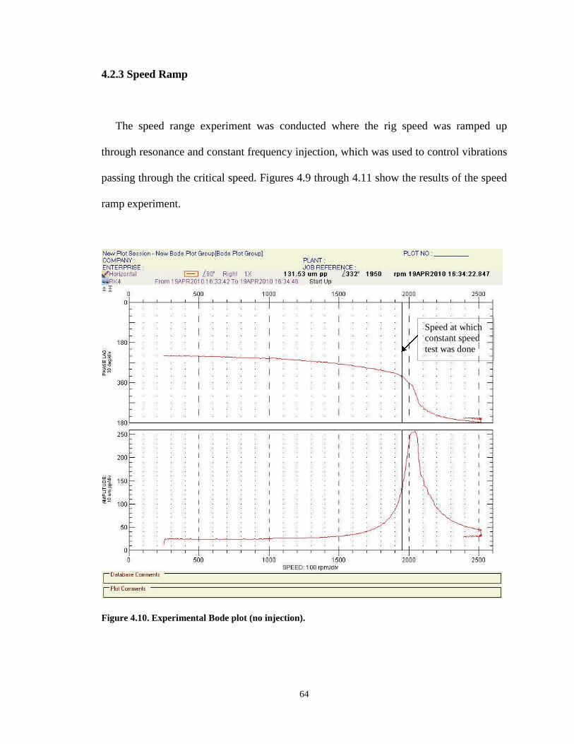
64
4.2.3 Speed Ramp
The speed range experiment was conducted where the rig speed was ramped up
through resonance and constant frequency injection, which was used to control vibrations
passing through the critical speed. Figures 4.9 through 4.11 show the results of the speed
ramp experiment.
Figure 4.10. Experimental Bode plot (no injection).
Speed at whichconstant speedtest was done
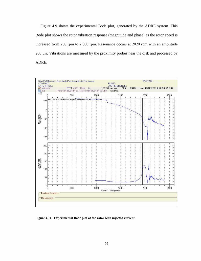
65
Figure 4.9 shows the experimental Bode plot, generated by the ADRE system. This
Bode plot shows the rotor vibration response (magnitude and phase) as the rotor speed is
increased from 250 rpm to 2,500 rpm. Resonance occurs at 2020 rpm with an amplitude
260 µm. Vibrations are measured by the proximity probes near the disk and processed by
ADRE.
Figure 4.11. Experimental Bode plot of the rotor with injected current.
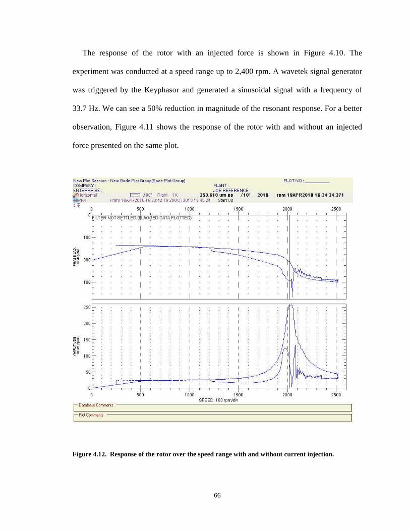
66
The response of the rotor with an injected force is shown in Figure 4.10. The
experiment was conducted at a speed range up to 2,400 rpm. A wavetek signal generator
was triggered by the Keyphasor and generated a sinusoidal signal with a frequency of
33.7 Hz. We can see a 50% reduction in magnitude of the resonant response. For a better
observation, Figure 4.11 shows the response of the rotor with and without an injected
force presented on the same plot.
Figure 4.12. Response of the rotor over the speed range with and without current injection.

67
Due to limitations of the equipment, it is not possible to adjust the frequency of the
injected generated signal in real time. At all speeds in the range of the experiment, the
generator produced a constant frequency wave for every revolution of the shaft. A better
result could probably be achieved if the generator could change the injection frequency
according to the rotational speed.
68
CHAPTER V
CONCLUSIONS
5.1 Summary
A novel method for vibration control of a flexible rotor using a feed-forward signal
and magnetic force actuator has been studied. The method was discussed and an
analytical solution of the required magnetic actuator current, to cancel the steady state
vibrations, was found. An experimental was discussed, including the generation of a
system transfer function using a finite element method and rotordynamics modeling of
the rig. A Campbell diagram, critical speed map, unbalance response simulation, and
mode shape analysis were done. The flexible rotor model was confirmed by the impulse
hammer modal testing method. The proper current was modified to be applicable for
readily available signal generator hardware and demonstrated to be effective using
numerical simulations. The vibration control method was confirmed by operating the at
a constant speed and at changing speeds and comparing its behavior with and without the

69
control method applied. An approximately 90% reduction in vibration amplitude was
achieved.
5.2 Contributions
The new method was proposed for the control of vibrations for a flexible rotor. The
method uses a magnetic actuator and feed-forward of single frequency harmonic current
signals which counteract the unbalance force. It is unique because of the simplistic
application of the harmonic control signal, but it maintains the practical effectiveness of
more complicated approaches. Because of this, the proposed method is more useful to
industry than the current methods, which require specialized hardware.
5.3 Future Research Directions
This work can be further developed in a few areas. Studies could be conducted to
examine the influence of the change of location of the actuator on the effectiveness of the
vibration control. For example, the actuator can be located at the main unbalance
location for the maximum effect, located near the bearing for minimum interference of
the machine function, or at other locations to control other modes of vibration. Also, this
method could be studied in a real world application by using an actual machine with
realistic unbalance issues as a . An important area of improvement is the creation of an
automated algorithm for injection tuning. This will speed the process and may be able to
achieve slightly greater levels of vibration cancelling.
Some problems have been analyzed in this work, and the results may now be
summarized. The following conclusions emerge.
70
A new method for the control of flexible rotor system vibration using an active
magnetic actuator was established. Going to this goal theoretical explanation of the
remodeled rotor was reviewed. This review lead to the more precise formula for force
and required current calculations.
The finite element model of the rig was developed. The modeling produced results
indicative of the actual rotor dynamic behavior.
71
REFERENCE
1. Alauze, C., Der Hagopian, J., Gaudiller, L., Voinis Ph., “Active Balancing of
Turbomachinery: Application to Large Shaft Lines,” Journal of Vibration and
Control, volume 7 no.2 p-p. 249-278, 2001
2. Burrows, C.R., Sahinkaya, N., Traxler, A., Schweitzer, G., “Design and
Application of a Magnetic Bearing for Vibration Control and Stabilization of a
Flexible Rotor,” Proceeding of the First International Symposium on Magnetic
Bearings, Zurich, June 6-8, 1988
3. Czolczynski, K., Rotordynamics of Gas-Lubricated Journal Bearing System,
Springer-Verlag, New York, Inc. 1999
4. Dimentberg, F.M., Flexural Vibration of rotating shafts, Butterworths’, London.
1961
5. Earnshaw, S., “On the Nature of the Molecular Forces witch Regulate the
Constitution of the Lumiferous Ether,” Trans. Of the Cambridge Philosophical
Society, Vol. 7, Part I, pp. 97-112. 1842
72
6. Ehrich, F., Handbook of Rotordynamics, McGRAW-HILL, Inc., New York. 1992
7. Findeisen, D., System Dynamics and Mechanical Vibrations, Springer-Verlag,
New York. 2000
8. Foppl, A., “The shaft of the Laval Steam-Turbine,” Der Civilingenieur pp.332-
342 1895
9. Genta, G., Vibration of structures and machines, Springer-Verlag. New York.
591p. 1999
10. Habermann, H., Liard, G., “Practical Magnetic Bearings,” IEEE Spectrum, Vol.
16, No. 9. September 1979
11. Jeffcott, H., “The lateral vibration of loaded shafts in the neighborhood of a
whirling speed-the effect of want of balance,” Phil. Mag., volume 37, no. 6, pp.
304-314. 1919
12. Kapitsa, P.L., “Ustoichivost I perekhod cherez kriticheskie oboroty bistro
vraschayschihsja rotorov pri nalichii treniya,” Zurnal teknicheskoi fiziki, IX,
Vypusk 2, 1939
73
13. Kasarda, M.E.F., Mendoza, H., Kirk, R.G., Wicks, A., “Reduction of
subsynchronous vibrations in a single-disk rotor using an active magnetic
damper,” Mechanics Research Communications, volume 31, issue 6, pp. 689–
695, 2004
14. Knospe C.R., Hope, R.W., Tamer, S.M., Fedigan, S.J., “Robustness of Adaptive
Unbalance Control of Rotors with Magnetic Bearings,” Journal of Vibration and
Control, volume. 2, no. 1, pp. 33-52, January 1996
15. Kramer, E., Dynamics of Rotors and Foundations, Springer-Verlag, New York,
1993
16. Krodkiewski, J.M., Sun, L., “Self-Tuning Adaptive Control of Forced Vibration
in Rotor Systems Using an Active Journal Bearing,” Journal of Sound and
Vibration, volume 231, pp. 1-14. 1998
17. Kai-Yew, L., Coppola, V. T., Bernstein, D. S., “Adaptive Auto centering Control
for an Active Magnetic Bearing Supporting a Rotor with Unknown Mass
Imbalance,” IEEE Transactions on control systems technology, volume 4, no 5,
September 1996
18. Muszynska, A., “Fundamental Response of a Rotor,” Bently Rotor Dynamic
Research Corporation, Minden, NV. 1986
74
19. Natanzon, V. Ya., “Frequencies of flexular vibration of a rotating shaft,”
Transactions of the Institute “Oborongiz”, no 142, 1948
20. Nelson, F.C., “Rotor Dynamic without Equations,” International Journal of
COMADEM, volume 10, no3, pp. 2 – 10, July 2007
21. Nikolai, E.L, “K teorii gibkogo vala,” Trud. Leningrad Ind. Inst., Razdelenie
Fiziki-Matematicheskikh Nauk, vypusk 3, no 6, 1937
22. Querioz, De M.S., “An Active Identification Method of Rotor Unbalance
Parameters,” Journal of Vibration and Control, volume 15, no 9, 2009
23. Rankine W. J. Mc. Q, “Centrifugal whirling of shafts,” The Engineer (London),
volume 26, April 8, p.249, 1869
24. Rayleigh, J. W., The theory of sound Volume 1, MacMillan, 2nd revised edition,
Cambridge, 1894
25. Sawicki, J. T., Fleming, D. P., Poplawski, J.V., “Unbalance Response Prediction
for Accelerating Rotors with Load-Dependent Nonlinear Bearing Stiffness,”
Third Biennial International Symposium on Stability Control of Rotating
Machinery (ISCORMA-3), 2005
75
26. Schweitzer, G., “Characteristics of a Magnetic Rotor Bearing for Active
Vibration Control,” First International Conference on Vibrations in Rotating
Machinery, 1976
27. Sun, J.C., Wang, X.G., Xi, F.J., “Sliding mode active vibration control of circular
saws,” International Conference on Control Applications, IEEE, pp. 953-958,
2000
28. Tammi, K., “Active Vibration Control of Rotor in Desktop Test Environment,”
Espoo VTT Publications 498, pp. 82-176, 2003
29. Timoshenko, S. P., “On the correction factor for shear of the differential equation
for transverse vibrations of bars of uniform cross-section,” Philosophical
Magazine, p. 744, 1921
30. Ulbrich, H., Elements of Active Vibration Control for Rotating Machinery, NASA
Lewis Research Center, Cleveland, Ohio, May 1990
31. Vance, J. M., Rotordynamic of Turbomachinery, John Wiley & Sons, New York,
1988
76
32. Yu, H-C, Lin, Y-H, Chu, C-L., “Robust modal vibration suppression of a flexible
rotor,” Mechanical Systems and Signal Processing, volume 21, pp. 334–347,
2007
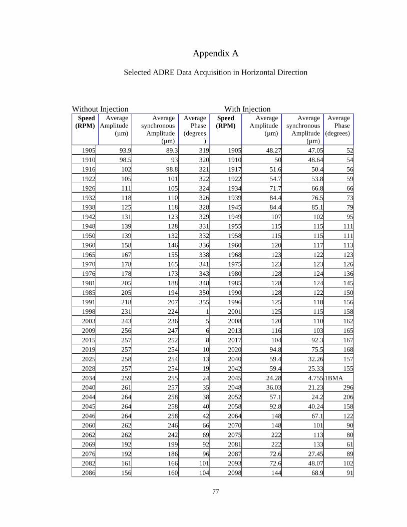
77
Appendix A
Selected ADRE Data Acquisition in Horizontal Direction
Without Injection With InjectionSpeed
(RPM)Average
Amplitude(µm)
Averagesynchronous
Amplitude(µm)
AveragePhase
(degrees)
Speed(RPM)
AverageAmplitude
(µm)
Averagesynchronous
Amplitude(µm)
AveragePhase
(degrees)
1905 93.9 89.3 319 1905 48.27 47.05 52
1910 98.5 93 320 1910 50 48.64 54
1916 102 98.8 321 1917 51.6 50.4 56
1922 105 101 322 1922 54.7 53.8 59
1926 111 105 324 1934 71.7 66.8 66
1932 118 110 326 1939 84.4 76.5 73
1938 125 118 328 1945 84.4 85.1 79
1942 131 123 329 1949 107 102 95
1948 139 128 331 1955 115 115 111
1950 139 132 332 1958 115 115 111
1960 158 146 336 1960 120 117 113
1965 167 155 338 1968 123 122 123
1970 178 165 341 1975 123 123 126
1976 178 173 343 1980 128 124 136
1981 205 188 348 1985 128 124 145
1985 205 194 350 1990 128 122 150
1991 218 207 355 1996 125 118 156
1998 231 224 1 2001 125 115 158
2003 243 236 5 2008 120 110 162
2009 256 247 6 2013 116 103 165
2015 257 252 8 2017 104 92.3 167
2019 257 254 10 2020 94.8 75.5 168
2025 258 254 13 2040 59.4 32.26 157
2028 257 254 19 2042 59.4 25.33 155
2034 259 255 24 2045 24.28 4.755151BMA
2040 261 257 35 2048 36.03 21.23 296
2044 264 258 38 2052 57.1 24.2 206
2045 264 258 40 2058 92.8 40.24 158
2046 264 258 42 2064 148 67.1 122
2060 262 246 66 2070 148 101 90
2062 262 242 69 2075 222 113 80
2069 192 199 92 2081 222 133 61
2076 192 186 96 2087 72.6 27.45 89
2082 161 166 101 2093 72.6 48.07 102
2086 156 160 104 2098 144 68.9 91
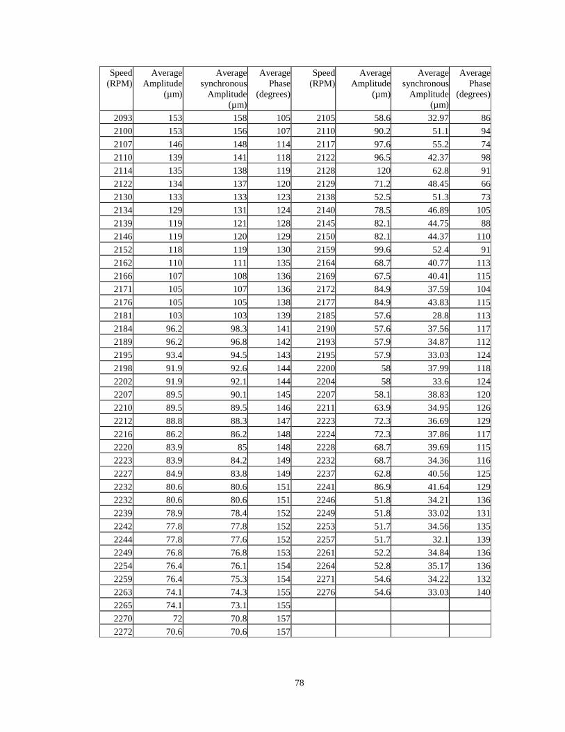
78
Speed(RPM)
AverageAmplitude
(µm)
Averagesynchronous
Amplitude(µm)
AveragePhase
(degrees)
Speed(RPM)
AverageAmplitude
(µm)
Averagesynchronous
Amplitude(µm)
AveragePhase
(degrees)
2093 153 158 105 2105 58.6 32.97 86
2100 153 156 107 2110 90.2 51.1 94
2107 146 148 114 2117 97.6 55.2 74
2110 139 141 118 2122 96.5 42.37 98
2114 135 138 119 2128 120 62.8 91
2122 134 137 120 2129 71.2 48.45 66
2130 133 133 123 2138 52.5 51.3 73
2134 129 131 124 2140 78.5 46.89 105
2139 119 121 128 2145 82.1 44.75 88
2146 119 120 129 2150 82.1 44.37 110
2152 118 119 130 2159 99.6 52.4 91
2162 110 111 135 2164 68.7 40.77 113
2166 107 108 136 2169 67.5 40.41 115
2171 105 107 136 2172 84.9 37.59 104
2176 105 105 138 2177 84.9 43.83 115
2181 103 103 139 2185 57.6 28.8 113
2184 96.2 98.3 141 2190 57.6 37.56 117
2189 96.2 96.8 142 2193 57.9 34.87 112
2195 93.4 94.5 143 2195 57.9 33.03 124
2198 91.9 92.6 144 2200 58 37.99 118
2202 91.9 92.1 144 2204 58 33.6 124
2207 89.5 90.1 145 2207 58.1 38.83 120
2210 89.5 89.5 146 2211 63.9 34.95 126
2212 88.8 88.3 147 2223 72.3 36.69 129
2216 86.2 86.2 148 2224 72.3 37.86 117
2220 83.9 85 148 2228 68.7 39.69 115
2223 83.9 84.2 149 2232 68.7 34.36 116
2227 84.9 83.8 149 2237 62.8 40.56 125
2232 80.6 80.6 151 2241 86.9 41.64 129
2232 80.6 80.6 151 2246 51.8 34.21 136
2239 78.9 78.4 152 2249 51.8 33.02 131
2242 77.8 77.8 152 2253 51.7 34.56 135
2244 77.8 77.6 152 2257 51.7 32.1 139
2249 76.8 76.8 153 2261 52.2 34.84 136
2254 76.4 76.1 154 2264 52.8 35.17 136
2259 76.4 75.3 154 2271 54.6 34.22 132
2263 74.1 74.3 155 2276 54.6 33.03 140
2265 74.1 73.1 155
2270 72 70.8 157
2272 70.6 70.6 157
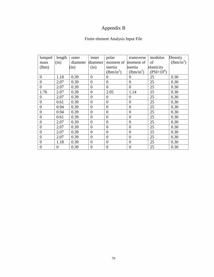
79
Appendix B
Finite element Analysis Input File
lumpedmass(lbm)
length(in)
outerdiameter
(in)
innerdiameter(in)
polarmoment ofinertia(lbm/in2)
transversemoment ofinertia(lbm/in2)
modulusof
elasticity(PSI×106)
Density(lbm/in3)
0 1.18 0.39 0 0 0 25 0.300 2.07 0.39 0 0 0 25 0.300 2.07 0.39 0 0 0 25 0.301.76 2.07 0.39 0 2.05 1.14 25 0.300 2.07 0.39 0 0 0 25 0.300 0.61 0.39 0 0 0 25 0.300 0.94 0.39 0 0 0 25 0.300 0.94 0.39 0 0 0 25 0.300 0.61 0.39 0 0 0 25 0.300 2.07 0.39 0 0 0 25 0.300 2.07 0.39 0 0 0 25 0.300 2.07 0.39 0 0 0 25 0.300 2.07 0.39 0 0 0 25 0.300 1.18 0.39 0 0 0 25 0.300 0 0.39 0 0 0 25 0.30
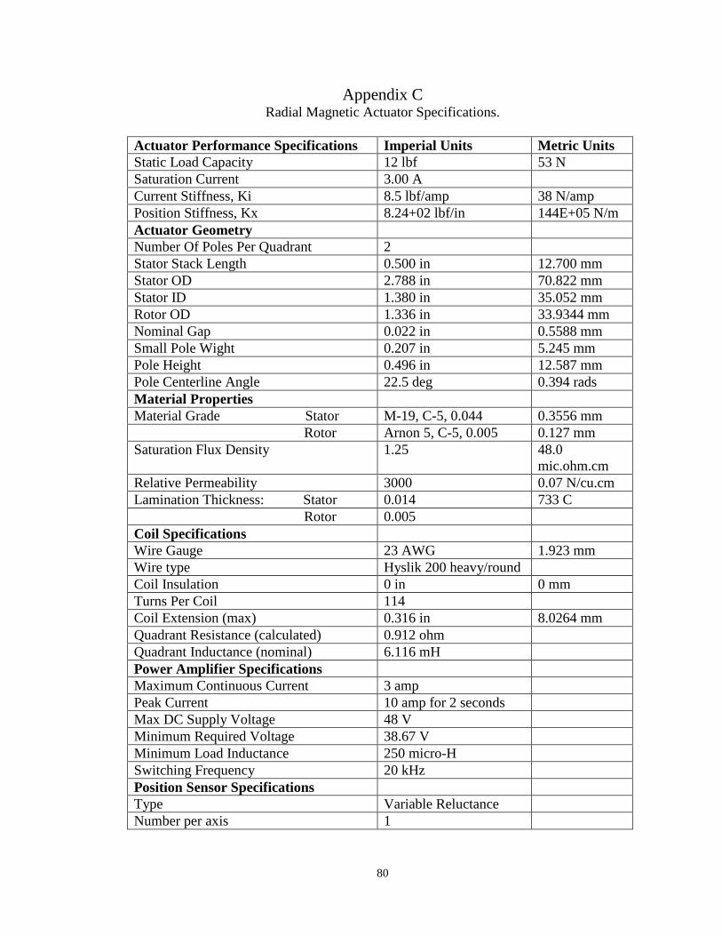
80
Appendix CRadial Magnetic Actuator Specifications.
Actuator Performance Specifications Imperial Units Metric UnitsStatic Load Capacity 12 lbf 53 NSaturation Current 3.00 ACurrent Stiffness, Ki 8.5 lbf/amp 38 N/ampPosition Stiffness, Kx 8.24+02 lbf/in 144E+05 N/mActuator GeometryNumber Of Poles Per Quadrant 2Stator Stack Length 0.500 in 12.700 mmStator OD 2.788 in 70.822 mmStator ID 1.380 in 35.052 mmRotor OD 1.336 in 33.9344 mmNominal Gap 0.022 in 0.5588 mmSmall Pole Wight 0.207 in 5.245 mmPole Height 0.496 in 12.587 mmPole Centerline Angle 22.5 deg 0.394 radsMaterial PropertiesMaterial Grade Stator M-19, C-5, 0.044 0.3556 mm
Rotor Arnon 5, C-5, 0.005 0.127 mmSaturation Flux Density 1.25 48.0
mic.ohm.cmRelative Permeability 3000 0.07 N/cu.cmLamination Thickness: Stator 0.014 733 C
Rotor 0.005Coil SpecificationsWire Gauge 23 AWG 1.923 mmWire type Hyslik 200 heavy/roundCoil Insulation 0 in 0 mmTurns Per Coil 114Coil Extension (max) 0.316 in 8.0264 mmQuadrant Resistance (calculated) 0.912 ohmQuadrant Inductance (nominal) 6.116 mHPower Amplifier SpecificationsMaximum Continuous Current 3 ampPeak Current 10 amp for 2 secondsMax DC Supply Voltage 48 VMinimum Required Voltage 38.67 VMinimum Load Inductance 250 micro-HSwitching Frequency 20 kHzPosition Sensor SpecificationsType Variable ReluctanceNumber per axis 1