Application Note 059

Advanced Microwave Amplifier Models and X-Parameter Simulation Setup Examples for Advanced Design System

Simulation

Introduction

This Application Note gives a tutorial overview of nonlinear amplifier models available from Modelithics™, with a focus on the enabling features of X-parameters models.

Mobile and wireless communication has seen phenomenal growth over the past two decades. Faster communication with higher data rates has been the driving factor. To achieve this, the RF front end components have been continuously improved to meet the linearity and power requirements and a range of wireless standards have emerged, based on variations in frequency, modulation and power level requirements. The 0.7 GHz to 6 GHz band has been the mostly widely used frequency range for mobile and wireless communications using different standards such as GSM, CDMA, WCDMA, LTE, WLAN and WiMAX. The evolving 5G standard is pushing frequency ranges for emerging commercial systems upward to mm-wave frequencies1 as high as 86 GHz! Still, the bulk of near term 5G developments will likely be at the proposed bands of 28GHz and below.

Amplifiers are an indispensable component of the circuitry for wireless and microwave systems. They have been used in a variety of applications including mobile communications, microwave heating, jamming and electronic warfare networks, radar systems and satellite communications. There are many vendors that manufacture low noise amplifiers, power amplifiers, gain blocks and variable gain amplifiers for microwave wireless frequency bands below 6 GHz. An increasing number of products are now also being offered at higher frequencies, including many GaN MMIC based amplifiers, which offer higher power densities and higher frequencies than possible with Silicon and GaAs power transistor technologies.

When it comes to modeling, among the most advanced models available for nonlinear simulations is the X-parameter*2 model3,4,5. This is conveniently supported within Keysight Advanced Design System (ADS) and Genesys. Another model that is available and predates X-parameters is the P2D model6,7. Both are behavioral models that are particularly useful for modeling productized die and packaged integrated circuit amplifiers, for which internal schematic details may not be available to the modeler. In the following treatment, examples of both models are discussed with an emphasis on the more powerful and accurate X-parameter model. X-parameter models can be generated either from an ADS nonlinear circuit simulation or from measurements taken on a suitably equipped test bench, such as one equipped with a nonlinear vector network analyzer (NVNA) like the Keysight PNA-X. Our focus in this article will be on measurement-generated models.

* X-parameters" is a trademark of Keysight Technologies, Inc. The X-parameters format and underlying equations are open and documented. For more information on the use of this trademark, refer to X-parameters Open Documentation, Trademark Usage & Partnerships. http://www.keysight.com/find/eesof-x-parameters

2

Available Models

Table 1 shows a list of currently available amplifier models included in the Modelithics™® COMPLETE Library for ADS. These models are setup to enable both broad-band linear as well as nonlinear simulations of internally matched and unmatched amplifiers. Many of the models include noise parameter prediction and all allow some level of nonlinear simulations with the X-parameter model being most flexible and accurate. Several of these models are also available for immediate free use thanks to sponsorship from Mini-Circuits. Unique model features test conditions and simulation results along with measurement validations, are detailed in each models’ data sheet. The columns to the right of the product listing in Table 1 indicate various features of these models that use either the X-parameters or the P2D model. Note one Modelithics™ model, for the Qorvo RF2878, includes both X-Parameter and P2D model formats7, that can be selected by setting the user-defined parameter to 0 for P2D and 1 for X-Parameters. This model is available in Modelithics™ SELECT+ free sample library for ADS. While the focus in this article will be on models for ADS, X-parameters-based models are also available from Modelithics™ for Keysight Genesys.

Table 1. Currently Available Models as Included in Modelithics™ COMPLETE Library for ADS

Vendor Part Number Modelithics Model Number Body Style

Max Freq.

(GHz)

P1dB

(dBm) No

n-L

inea

r

X-P

aram

eter

s M

od

el

P2D

Mo

del

Sub

stra

te S

cala

ble

No

ise

Par

amet

ers

Bro

adb

and

S-P

aram

eter

s

Tem

per

atu

re D

epen

den

t

Load

Pu

ll

TOI

Free

Do

wn

load

s

Avago MGA-635P8 AMPXP-AVA-MGA635P8-001 2x2mm QFN 13 22

Avago MGA86576 AMP-AVA-MGA86576-001 Package 10 7

Freescale MWE6IC9100NR1 AMPXP-FRS-MWE6IC9100NR1-001 TO-270 0.96 50

Guerrilla RF GRF2070DS AMPSP-GUR-GRF2070-001 2x2mm DFN 8 20.1 *

Guerrilla RF GRF2071DS AMPSP-GUR-GRF2071-001 2x2mm DFN 8 21 *

Guerrilla RF GRF2072DS AMPSP-GUR-GRF2072-001 2x2mm DFN 8 19.7 *

Guerrilla RF GRF2073DS AMPSP-GUR-GRF2073-001 2x2mm DFN 8 18 *

Guerrilla RF GRF2501DSR AMPSP-GUR-GRF2501-001 1.5x1.5mm DFN 8 -8 *

Maxim MAX2371 AMP-MAX-2371-001 QFN 2.5 -3

Maxim MAX2373 AMP-MAX-2373-001 QFN 2.5 -3

Mini-Circuits GVA-62+ AMPXP-MCL-GVA62+-001 SOT-89 18 19.8

Mini-Circuits GVA-63+ AMPXP-MCL-GVA63+-001 SOT-89 18 19

Mini-Circuits GVA-84+ AMPXP-MCL-GVA84+-001 SOT-89 12 20.5

Mini-Circuits PGA-102+ AMPXP-MCL-PGA102+-001 SOT-89 12 17.5

Mini-Circuits PGA-103+ AMPXP-MCL-PGA103+-001 SOT-89 12 22.5

Mini-Circuits PGA-105+ AMPXP-MCL-PGA105+-001 SOT-89 12 19.3

Mini-Circuits PHA-1+ AMPXP-MCL-PHA1+-001 SOT-89 18 22

Mini-Circuits PHA-22+ AMPXP-MCL-PHA22+-001 DL1020 12 22

Mini-Circuits PSA4-5043+ AMPXP-MCL-PSA4-5043+-001  SOT-343 12 21

Mini-Circuits ZFL-1000LN+ AMP-MCL-ZFL-1000LN+-001  Coaxial 1 3 *

NEC uPC8179TK-E2-A AMP-NEC-UPC8179TK-001 1151 Minimold 2.4 2

Qorvo AH101 AMPXP-TQT-AH101-001 SOT-89 15 26.5

Qorvo RF2132 AMP-RFMD-RF2132-001 Package 3 29

Qorvo RF2878 AMPXP-RFMD-RF2878-001 Package 3 14.4

Qorvo RF5110G AMPXP-RFMD-RF5110G-001 3x3mm QFN 3 36

Qorvo TGA8344-SCC AMP-TRI-TGA8344-001 MMIC 26 16

Qorvo TGA8399B-SCC AMP-TRI-TGA8399B-001 MMIC 10 11

Qorvo TGA8810-SCC AMP-TRI-TGA8810-001 MMIC 13 17

*In development, available for pre-release ordering.

3

Understanding X-Parameters (In Brief)

X-Parameters are analogous to S-Parameters. They are both behavioral or “black box” models, in that there is no need for knowledge of internal circuitry, design or device type. However, whereas S-parameters provide for linear input/output relationships, X-parameters enable multi-harmonic nonlinear simulations. X-parameters can be easily ported to multiple EDA platforms, but like S-parameters performance one must be very careful about any extrapolations in frequency, power, or bias outside of the data range used to build the model. Modelithics™ X-parameter model datasheets give power, frequency, bias, and additional guidelines for model users. As Figure 1 suggests a behavioral model provides a nonlinear mapping between a time domain (or multi-harmonic frequency domain) input signal x(t) and output signal y(t). Shown also is the Modelithics™ X-parameters-based model representation for a specific example amplifier model from Mini-Circuits. The available input parameters will vary with the model. The “model_mode” parameter is set to “1” for nonlinear X-parameter analyses and to “0” for small-signal S-parameter analyses. For practical reasons, it is easier to provide a broader-band small-signal (S-parameter-based) model to include out of band frequencies that may be of interest for stability and other purposes. The nonlinear model will generally be applicable to a narrower frequency band, including the main operating band of interest, since it is more “expensive” to develop in terms of test time and measurement complexity. This is especially true when measuring X-parameters of high power devices and circuits.

Figure 1. Amplifier representation as a “black box” model: a. packaged amplifier shown with desired mapping between output y(t) and input x(t), b. Modelithics™ ADS model for GVA84+ amplifier from Mini-Circuits.

4

Whereas a deep dive on the mathematical formulation of X-parameters is beyond our scope here it may be helpful to review in brief one of the main defining equations shown below in Eq.. 1.

Equation 1

Before we discuss the terms in Eq. 1, let’s recall the form of the S-parameter formulation that X-parameters simplify to in the low power linear extrapolation. Eq. 2 should look more familiar, and friendly!

Equation 2

or

Equation 3

Starting with Eq. 2, b1 and b2 are the “reflected” voltage waves flowing out of ports 1 and 2, respectively, from a 2-port device, defined in terms of the S-parameters and the incident voltage waves a1 and a2. The indices 1 and 2 are port indices and all parameters are frequency dependent. This is a linear equation set and no new frequencies are generated and the “mapping” is assumed to be amplitude independent. The S-parameters are measured as ratios between reflected and incident waves, typically using a vector network analyzer, with no need to know the exact absolute power level of any of the waves. Eq. 3 is equivalent to Eq. 2 with i and j being the input and output port indices, respectively. S-parameters models obey superposition, that the combination of multiple small signal stimuli presented to the model will output the same response as the sum of the individual responses would. As such, S-parameters are easily and conveniently cascaded in a linear mode of operation.

Turning our attention to Eq. 1, in this case we have a nonlinear mapping between “reflected” or outgoing “b” waves, linear superposition does not apply and we have new periodic frequencies generated, cross frequency phase dependency, and the mapping is amplitude and frequency dependent at a single operating point. For this reason, there are four subscript indices used in the equation: i is the output port index, j is the output frequency (or harmonic number) index, k is the input port index and l is the input frequency (or harmonic number) index. This formulation is setup to accurately represent amplitude dependence under the variance of port 1 power as represented by the notation |A11|, which is the amplitude of the incident wave on port 1 at the fundamental frequency. The X-parameters are the functions that have superscripts (F), (S) and (T) and depend nonlinearly on |A11|. P is a phase term that, along with the magnitude-only dependence on |A11| of the X(S) and X(T) functions, is a necessary consequence of the assumed time invariance of the underlying system5. When measuring X-parameters with a modern nonlinear vector network analyzer, such as a suitably optioned Keysight PNA-X, we need to calibrate for and accurately measure absolute powers

)1,1(,

*

11

)(

,11

)(

,11

)( ))()(()(lk

kl

ljT

klijkl

ljS

klijj

F

ijij aPAXaPAXPAXb

2221212

2121111

aSaSb

aSaSb

2 ,1for 2

1

iaSbk

kiki

5

and the phase relationship at fundamental and all harmonic frequencies to be recorded. Moreover, for high efficiency amplifiers or when PAE is important, drain efficiency data can be included in the X-parameter model by carefully setting up the bias in the NVNA menu to establish communication between instruments and guaranteeing that the model is set up properly with measurement variables8.

The motivated and mathematically inclined reader is referred to the cited references to dig deeper into understanding Eq. 1; however, some graphical insight is offered in Figure 2. For engineers who have a lot of familiarity looking at S-parameters for amplifiers, a first look at X-parameters plotted can be far from intuitive! Nevertheless, when we consider that X-parameters are a superset of S-parameters, we can start getting some comfort level by examining Figure 2a. Note how some of the functions can be presented in a way that directly correlates with the more familiar S11 and S21 parameters at low power. Figure 2b, illustrates the multi-frequency, multi-port mapping that X-parameters enable between the nonlinear a and b waves. One of the key advantages to X-parameters is the way that harmonic signals with accurate harmonic amplitude and phase information are captured. This enables time domain waveform transformations as well as accurate analysis of cascaded nonlinearities. This contrasts with the worst-case system analysis performed by engineers for many years, using traditional spread-sheet methods.

6

a.

b.

Figure 2. Graphical views to assist with understanding X-parameters for an amplifier: a. in terms of linear extrapolation to S-parameters and b. representation of the multi-port/multi-harmonic frequency mapping the X-parameters enable. (Graphics provided courtesy of Keysight Technologies.)

X-parameters enable accurate analysis of multi-stage or cascaded nonlinearities,

not just worst-case analysis

7

Figure 4. Location of the open workspace button on the ADS main window.

Example Amplifier Models and Simulation Results

We now turn to presenting a few examples of X-parameter models selected from Table 1. We will start with the GVA84+ model. Figure 3 illustrates the Modelithics™ datasheet available for this amplifier model.

Loading the Example Workspace

Accessing Modelithics™ amplifier examples is a straightforward process. Once one of the featured Modelithics™ libraries have been installed to the system, the examples folder will be available to access within the Modelithics™ library folder on the computer.

Opening the main ADS window; navigate to the ‘Open Workspace’ button or select it in the dropdown menu by going to File -> Open-> Workspace.

Figure 3. As an example, the Modelithics™ datasheet for the GVA84+ model contains 15 pages of information on model use, validations and detailed technical information.

8

Once selected, to open a workspace, navigate in the ‘Open Workspace’ window to “C:\Modelithics\Examples_forKeysightADS\SLC\Workspaces”. Note: if you chose a different

directory other than the default path to install your Modelithics™ library the folder path will be slightly different than above.

Within the Workspaces folder there will be a list of example workspace projects to choose from. Once opened, the workspace will contain schematics and plots for the available simulations with that model. These tests are designed to replicate the information contained in each models’ datasheet. These tests include S-parameter, noise, 1dB compression sweeps, single tone power sweeps, and 2 Tone Power Sweeps.

For this example, select the workspace labeled “Mini-Circuits_GVA84plus_ExampleProject_wrk” and open it.

Figure 5. The ADS open workspace window with the available Modelithics examples displayed.

Figure 6. Once the example for GVA84+ has been opened this will be displayed in the main ADS window. Depending on your setting the arrangement of files may be different.

9

Model Parameters for X-parameter amplifier models

Many of the X-parameter models in the Modelithics™ library are designed to work under conditions specified by the manufacturer of the physical part. Some of the X-parameter amplifiers have editable parameters such as voltage biasing, substrate scaling, and model modes. These parameters can be altered according to the user’s requirements. Listed below are the Mini-Circuits X-parameter models that are currently available for use.

Table 2. A listing of all available Mini-Circuits models available in Modelithics libraries.

Table of Modelithic Mini-Circuit Models

Model Bias Substrates Freq Range

MCL-62+ +5V 20mil Rogers 0.05-18 GHz

MCL-63+ +5V 20mil Rogers 0.05-18 GHz

MCL-84+ +5V 10mil Rogers 0.05-12 GHz

MCL-PGA102+ +3.3V 10mil Rogers 0.05-12 GHz

MCL-PGA103+ +3V or +5V 10mil Rogers 0.05-12 GHz

MCL-PGA105+ +5V 10mil Rogers 0.05-12 GHz

MCL-PHA1+ +5V 20mil Rogers 0.05-18 GHz

MCL-PHA22+ +5V 10mil Rogers 0.05-12 GHz

MCL-5043+ +3 or +5V 10mil or 30mil Rogers 0.1-12 GHz

Parameters on models

Some of the Modelithics™ amplifier X-parameter models can simulate over bias. These models have a voltage (V) parameter included with them that allows the user to specify the desired voltage to be applied in simulations (within a range specified in the model data sheet). The available biases and their ranges can be found within each individual model datasheet. Consult the model features on the top of the first page for a brief overview of available voltage settings for each model.

Figure 7. The Mini-Circuits 5043+. This amplifier model has both bias and substrate scaling available as well as the standard model mode.

10

Also available on some Modelithics™ X-parameter models is the ability to scale with substrate. Models that have this scalability have an “H” and “Er” user parameter. These parameters set the height and dielectric constant of the substrate to be included in the simulation. Each substrate scalable model has been measurement validated and will scale across the H/Er range specified in the datasheet. It is recommended to consult the models’ datasheet for more technical information on substrate scaling when available.

The model_mode parameter is found on all Modelithics X-parameter amplifier models and is used to dictate the modeling type the amplifier will be used for. This parameter currently has two settings available to switch the model between linear simulation mode and non-linear simulation mode. Its’ setting is dependant upon the requirements of the simulation being performed.

Simulations with X-Parameter Models Linear Simulations (model_mode = 0) - The model, which is setup using the manufacturer recommended bias point of 5V and low power current of 108mA, has two model modes: 0 and 1. Model mode 0 enables accurate linear S-parameter simulation over 0.05 to 12 GHz. Noise parameter prediction is also provided for over 0.5 to 6 GHz, using the same mode. Figure 8 shows simulated and measured S-parameter and noise parameter results for the GVA84+ amplifier model. One of the advantages of data-based behavioral models like S-parameters and X-parameters models, is that agreement to measured data can be exact “on grid” (that is when the simulation corresponds to measured data conditions used in generating the model.)

Figure 8. S-parameters (a.) and noise parameters (b.) simulation and measured results for GVA84+ model using model_mode=0 setting and appropriate linear ADS simulation schematics.

11

Linear Simulations: S-parameters and Noise Workspace

Performing a linear simulation with the models begins by opening the “Sparameter and NoiseSim” schematic for a given workspace. The frequency of the schematic is set to reflect the range covered in the model datasheet. In this example, the GVA84+ is accurate for S-parameters from 0.5 to 12 GHz and accurate for Noise simulations from 0.5 to 6 GHz. Note that the amplifier is set to model_mode=0.

In this schematic, the frequency range for noise simulations is set by placing a S-Parameter block from the palette menus and setting the start and stop frequencies from 0.5 to 6 GHz. Step size can be defined by the user’s preference in this case we will be using a 50 MHz step.

Included in the schematic is the DisplayTemplate block for “S_Params_Quad_dB_Smith”. This block automatically plots S-parameters and Noise parameters.

Full S-parameter results are displayed on the left side of the default display. Noise results are only included on the right side of the page displaying Noise and Minimum Noise, Noise Resistance, and the Gopt of the simulated model.

Each model has unique frequency ranges that can be found in each models’ datasheet. It is not recommended to simulate behavioral models, like X-parameters, outside of the specified

Figure 10. The S-Parameter Sweep and DisplayTemplate blocks.

Figure 9. The example S-parameter and Noise simulation schematic.

12

range as this will result in extrapolation.

Nonlinear HB Simulations (model_mode=1) - Switching to nonlinear analysis, Figure 11 shows simulation results for a single-tone power sweep setup for the same amplifier model. According to the model datasheet, nonlinear analysis can be performed from 0.2 to 6 GHz. As can be seen in Figure 11, the device is compressed at high-power levels. Since X-Parameters contain information about the device’s amplitude and phase at multiple harmonics, the nonlinear phase behavior (e.g. AM/PM) in the compression region can also be assessed. The results of using a somewhat more involved simulation setup for P1dB calculated across a range of frequencies are shown in Figure 12Figure 12, with excellent correlation to the manufacturer’s specified P1dB for this part.

Figure 11. Multi-harmonic power sweep simulation for GVA84+ amplifier example showing amplitude and phase at 2GHz for the b2j (amplifier output signal) wave at j= 1, 2 and 3, corresponding to fundamental (red), second (blue) and third (green) harmonic.

Legend: Red: Fundamental Output Power at P1dB, Blue X: Mini-Circuits: Measured Typical Data Plot shows P1dB vs. Frequency X-Parameter Model results mounted on 10mil Rogers 4350B substrate. DC Voltage: +5V, model_mode=1 used.

Figure 12 Simulated results for cross-frequency 1dB compression power simulations compared to manufacturers

13

data.

Non-Linear Simulations: Single Tone Power Sweeps & Power Compression

The example workspace comes with several single tone harmonic balance schematics. Typically, there is one schematic per simulated result in the models’ datasheet. Each model datasheet provides a list of available dBm power ranges that the amplifiers function in depending on the frequency selected for simulation. For this example, the schematic chosen will simulate at 2000 MHz. For this, we need to open the “1tonePswp_HBsim_2000MHz” schematic.

In this schematic, the circuit has again been setup with a completed circuit including two current probes for measurements as well as a 1 tone terminal block at port 1. This block allows for an adjustable input frequency and power.

Observing the Harmonic Balance block, there are inputs for frequency and the number of harmonics to be simulated. In this schematic, the frequency refers to a fundamental frequency which has been defined along with a default input power (Pin) for the 1 tone terminal block. A Parameter Sweep block has also been added to the schematic to sweep the Pin

Figure 14. Harmonic balance and parameter sweep blocks.

Figure 13. Example single tone power sweep schematic. Note the current probe positions and parameter blocks.

14

parameter while during simulation.

Simulating the schematic, input power is swept from the datasheet specified range of -10 to 5 dBm for our chosen frequency. To properly display the forward transmission and output power of the simulated model a few equations must be observed.

These equations represent the formula for forward transmission power, dBm(a1) and phase, phase(a2), as well as the output power, dBm(b1) and its respective phase, phase(b2). To properly display the second and third orders of the output power, the plots must be specified for each order.

Another single tone simulation available for X-parameter models are power compression simulations. These have a similar setup to the Harmonic Balance simulation but include the addition of a ‘Gain Compression’ block to the schematic. This block has the ability to constrain a number of the parameters during simulation. The Gain Compression block requires a definition of the input and output ports as well as the desired input and output frequency. Also included are restrictions for power variation and the maximum allowed input power (measured in dBm) to be used during simulation.

Nonlinear Envelope Domain Simulations (model_mode=1) Another common amplifier figure of merit of interest is two-tone third order intermodulation (IM3) and third order intercept point (IP3) simulations. While there is a methodology for measuring X-parameters under 2-tone simulation9, our scope here

will be limited to X-parameters generated from more conventional 1-tone X-parameters test setups. That said, our experience in validations done so far is that quite good results can be obtained for 2-tone IM3 and IP3 simulations using 1-tone X-parameters models, with certain caveats also observed10. Figure shows that excellent results were obtained for this comparison between simulated and measured third order distortion. In this case, the measurements were made at Modelithics™ using a separate test setup from that used to generate the X-parameters model. The envelope domain can also be used along with the same X-parameters model type to simulate more complex digital modulations, such as CDMA.

Another interesting example of the advantage of an X-parameter model over than that of an S-parameter model is one where superposition breaks down, such as two amplifiers, with non-linearities present, are cascaded as depicted in the schematic in Figure a, with simulated results shown below in Figure b. In this example, two X-parameter models of different Mini-Circuits XFL-1000LN+ amplifier units are cascaded back to back (AMP1 and AMP2). The

Figure 15. Equations that result in output power and phase.

Figure 16. Adding a gain compression block to a power sweep schematic allows for a power compression simulation.

15

results are then compared to a third X-parameter model (AMP3) where the cascaded amplifiers were treated as a single gain block and modeled together. AMP1 overdrives AMP2 at higher power levels, but unlike S-parameters, these X-parameter models are able to accurately predict the fundamental and harmonic spectra of the incoming and outgoing waves. This can be seen by observing the close correlation of the simulated results, verifying the accuracy of X-parameters with for proper calculation of cascaded non-linearities in both amplitude and phase.

a. Schematic block diagrams of AMP1 and AMP2 discrete X-parameter models cascaded in simulation (upper schematic) and the AMP3, which is the X-parameter model of the two amplifiers measured and modeled together as a discrete gain block.

b. Comparison of simulated results of an X-parameter model of cascaded amplifiers (red) to the result of a combination of the amplifiers when measured and modeled as individual X-parameter models (blue), and cascaded in simulation. Left plot shows simulated output power of the fundamental, 2

nd and 3

rd harmonics vs. input power. Right plot shows simulated phase

of the fundamental, 2nd

and 3rd

harmonics. 1 Ghz is the frequency of simulation.

Figure 17 Schematic (a.) and simulated results (b.) for output power and phase of the fundamental, 2nd

and 3rd

harmonics when two X-parameter amplifier models are cascaded together as measured and in simulation.

16

Figure 18 Simulation results compared to independently measured IP3/IM3 data. Left plot shows simulated IP3 vs. frequency over 0.2 to 3 GHz. Right plot shows power swept fundamental and IM3 data at 1 GHz fundamental for GVA84+ model.

Non-Linear Simulations: Two-tone Envelope Power Sweep

Two-tone power sweeps are also available within the example workspaces. These two-tone

simulations provided by the 1 tone X-parameter models are reliable representations of IM3

and IP3 simulations. Open the schematic labeled “2TonePswp_Envelope”. This schematic will

provide both IM3 and IP3 results once simulated in ADS.

The schematic of the two-tone circuit layout features a single current probe and a P_nTone

terminal connection for port 1. This nTone terminal can support multiple input frequency and

powers to represent up to the nth tone required. In this case the schematic calls for two

separate tones for simulation. For complex power sweeps such as this example, an Envelope

Figure 19. The example two-tone power sweep schematic.

17

block is used. This block is designed for use in high-frequency amplifiers that involve transient

or modulated RF signals. In this case we will be using it for RF modulated signal of two

separate signal inputs. The Envelope defines the frequency and the number of orders to be

simulated. The Envelope also defines the stop and step timings of transient calculations.

Since a two-tone schematic requires two unique inputs, the setup utilizes two separate

Parameter sweep blocks to simultaneously sweep both input frequency and the power of the

input signal. Using the nTone terminal, two equations are used to separate the signal from

each other without cluttering the schematic with too many variables. The same method is

used for the power

input of the circuit. In

this case, the RFpower

of both input signals

will be the same.

Consult the models’

datasheet for further

information on

appropriate input

frequency and power

combinations.

The simulation equations

shown are used to plot the

fundamental and third order

power output as well the IP3

results.

Load-Pull X-parameters Models - For the remaining examples we will switch to a different model. The previously discussed GVA84+ is a pre-matched amplifier that is matched in the

Figure 20. Blocks for configuring the envelope simulation. These blocks are used to set the constraints of the two-tone simulation.

Figure 21. Envelope simulation parameter sweeps used to define the ranges of power and frequency.

Figure 22. Equations used to define fundamental, third order, and IP3 results.

18

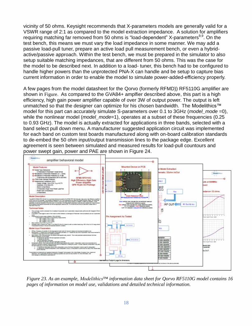
vicinity of 50 ohms. Keysight recommends that X-parameters models are generally valid for a VSWR range of 2:1 as compared to the model extraction impedance. A solution for amplifiers requiring matching far removed from 50 ohms is “load-dependent” X-parameters9,9. On the test bench, this means we must vary the load impedance in some manner. We may add a passive load-pull tuner, prepare an active load pull measurement bench, or even a hybrid- active/passive approach. Within the test bench, we must be prepared in the simulator to also setup suitable matching impedances, that are different from 50 ohms. This was the case for the model to be described next. In addition to a load- tuner, this bench had to be configured to handle higher powers than the unprotected PNA-X can handle and be setup to capture bias current information in order to enable the model to simulate power-added-efficiency properly. A few pages from the model datasheet for the Qorvo (formerly RFMD)) RF5110G amplifier are shown in Figure. As compared to the GVA84+ amplfier described above, this part is a high efficiency, high gain power amplifier capable of over 3W of output power. The output is left unmatched so that the designer can optimize for his chosen bandwidth. The Modelithics™ model for this part can accurately simulate S-parameters over 0.1 to 3GHz (model_mode =0), while the nonlinear model (model_mode=1), operates at a subset of these frequencies (0.25 to 0.93 GHz). The model is actually extracted for applications in three bands, selected with a band select pull down menu. A manufacturer suggested application circuit was implemented for each band on custom test boards manufactured along with on-board calibration standards to de-embed the 50 ohm input/output transmission lines to the package edge. Excellent agreement is seen between simulated and measured results for load-pull countours and power swept gain, power and PAE are shown in Figure 24.

Figure 23. As an example, Modelithics™ information data sheet for Qorvo RF5110G model contains 16

pages of information on model use, validations and detailed technical information.

19

Figure 24. Load-pull (left) and power swept nonlinear data (right) for Qorvo RF5110G amplifier

Non-linear Simulation: X-parameter Load Pulls

OPTIONSPAR AM ETER SW EEP H AR M ON IC B ALANCE

VarEqn

VarEqn

Var

Eqn

VarEqn

VarEqn

VarEqn

MLIN

I_Probe

S1P_EqnDC_Block

VAR

V_DC

I_Probe

DC_Feed

VAR

P_1ToneDC_Block

HarmonicBalance

VAR

ParamSweepOptions VAR

VAR

VAR

AM P XP_RFMD_RF5110G_001_MDLXSLC1

MTAPER MTAPER

Iload

S1DC_Block2

VAR101

SRC1

Is_high

DC_Feed1

TL1

SweepEquations10

PORT1DC_Block1

HB1

VAR50

Sweep1Options1 ImpedanceEquations1

VAR102

STIMULUS13

X1

Taper1 Taper2

Z[1]=Z0

S[1,1]=LoadTuner

Temperature=25

Vdc=Vhigh

Subst="MSub1"

W=0.000625 meter

L=0.0025 meter

Z0=50

pts=500

s11_center= -0.6-j*0.05

s11_rho =0.3

Freq=RFfreq

P=dbmtow(Pavs)

Z=50

Num=1

Order[1]=26

Freq[1]=RFfreq

Z_s_3 =Z0*(1+GammaS3)/(1-GammaS3)

Z_s_2 =Z0*(1+GammaS2)/(1-GammaS2)

Z_s_fund =Z0*(1+GammaS)/(1-GammaS)

Z_s_bb=Z0

;Source Impedances=

Z_l_3 =Z0*(1+GammaL3)/(1-GammaL3)

Z_l_2 =Z0*(1+GammaL2)/(1-GammaL2)

Z_l_bb=Z0

;Load Impedances=

MaxWarnings=10

GiveAllWarnings=yes

I_AbsTol=1e-5 A

I_RelTol=3e-5

V_AbsTol=1e-5 V

V_RelTol=3e-5

Tnom=25

Temp=25

GammaL3=-0.18878 +j*0.87158

GammaL=0

GammaL2=-0.69028 +j*0.59868

GammaS3=-0.00522 -j*0.00296

GammaS2=-0.00187 -j*0.00306

GammaS=0.05469 +j*0.02841

Vlow=0

Vhigh=3.6

RFfreq=0.26 GHz

Pavs=-5

Model_Mode=0 - Small Signal Model

RFfreq=RFfreq

E xtrapolation_Mode=1 - Interpolation

Band_Select=0 - 220 MHz Application Circuit

Subst="MSub1"

W1=25.0 mil

W2=20.0 mil

L=100.0 mil

Subst="MSub1"

W1=25.0 mil

W2=20.0 mil

L=100.0 mil

vload

Vs_high

v2

Running a load pull simulation requires a number of predefined variables in order to be

Figure 25. The schematic setup for the Qorvo RF5110G for load pull simulations. For this model, microstrip tapers are included to replicate the device in a circuit application.

20

successful. This circuit uses two separate inputs for simulation and need to be defined by the user during setup. The input frequency is inserted from the 1Tone port block and mixed with a DC voltage offset that is input to the system to supply a constant voltage that will not interfere with the A/C input. This DC offset defines the Bias of the system, in the case of this model the offset is 3.6V.

Additional to the harmonic balance and parameter sweep blocks used to sweep the frequency variable of the schematic, an options block is also used. This block allows control of simulation model temperatures, voltage and current tolerances, and a restriction to the number of warnings the simulation can produce during a given simulation. This does not limit the simulator from testing in these warning areas, it only restricts the number of warning messages the user will receive during simulation.

For load pull simulation, source and load gamma must also be defined within the schematic. These are uniquely dependent on the frequency at which the simulation will be run at and can be represented in a complex or polar format. Consulting the models’ datasheet will provide more information on the relationship of gamma source and load values to frequency and power input selections for the various load pull simulations.

Once simulated, the default display area will be controlled by one of the schematic variable blocks. This set of variables define the areas of a smith chart that will display the PAE and delivered power contours after the simulation has finished. These variables are necessary to translate the schematic inputs to data that can be represented on a smith chart at the users’ reference impendences, and within the constraints of the defined length and area specified by the variables defined in the schematic

of the load pull.

Summary

A library of advanced nonlinear models for a range of amplifier products is available for use in Keysight ADS. Advanced features include accurate de-embedding to device or package terminals with the same model being usable for broad-band linear and noise (where applicable) simulations as well as harmonic balance and envelope domain simulations enabled primarily by X-parameters technology. X-parameters are an excellent model solution for amplifier modeling. Among other reasons it requires little or no detailed internal device information and allows the amplifier to be treated as a black box. When extracted properly, the

OPTIONS

VarEqn

VarEqn

VAR

Options

VAR

SweepEquations10

Options1

STIMULUS13

Z0=50

pts=500

s11_center=-0.6-j*0.05

s11_rho =0.3

MaxWarnings=10

GiveAllWarnings=yes

I_AbsTol=1e-5 A

I_RelTol=3e-5

V_AbsTol=1e-5 V

V_RelTol=3e-5

Tnom=25

Temp=25

Vlow=0

Vhigh=3.6

RFfreq=0.26 GHz

Pavs=-5

VarEqn VAR

VAR102

GammaL3=-0.18878 +j*0.87158

GammaL2=-0.69028 +j*0.59868

GammaL=0

GammaS3=-0.00522 -j*0.00296

GammaS2=-0.00187 -j*0.00306

GammaS=0.05469 +j*0.02841

Figure 26. Options and variable definitions

for a typical load pull simulation

Figure 27. A variable block defining the

various gamma source and load values

used in a load pull simulation.

21

result is a model that can be used for multi-stage nonlinear analyses and design optimizations of individual amplifier output or inter-stage matching circuits.

Information and simulations from example models were used to illustrate the type of simulations that are provided for with each model. Specific examples of how to perform various simulations in ADS is also included to make it easy for designers to get up and running quickly with these simulations. To increase confidence we have also provided a range of measurement validations showing excellent correlations are possible with nonlinear test data, even if derived from completely independent test benches and verifying test data not used as part of the model development data set.

Acknowledgements and Additional Information

The authors would like to thank Keysight Technologies for collaboration related to this work as part of the Keysight Solution Partnership program. In particular, we would like to thank Chad Gillease for his great technical support and Jose Civello of Keysight for his helpful editing comments.

A trial of Modelithics™® COMPLETE Library for ADS can be requested at: https://www.Modelithics™.com/model. For designer convenience, several ADS workspace examples, including the schematic setups for results illustrated in this article are included in the Modelithics EXEMPLAR (trial and university version) Library and Modelithics COMPLETE Library installations

For access to the Mini-Circuits sponsored models, including the amplifier models discussed in this work see: https://www.Modelithics™.com/mvp/minicircuits.

.

About this note

This application note was developed by Larry Dunleavy, Kevin Kellogg, and Joshua Lowe

Contact Information

For information about Modelithics’ products and services, please contact us at:

Modelithics, Inc.

3802 Spectrum Blvd., Suite 130

Tampa, FL 33612

Voice: 813-866-6335

22

Email: sales@modelithics.com

Web: www.modelithics.com

References

1 Y. Niu, y, Li, D. Jin, L. Su, A Vasilakos, “A survey of millimeter wave communications (mmWave) for 5G: opportunities

and challenges,” Wireless Networks, Nov. 2015, Vol. 21, pp2657-2676 . 2 X-parameters is a trademark of Keysight Technologies. www.keysight.com

3 J. Verspecht and D. Root, “Polyharmonic Distortion Modeling,” IEEE Microwave Magazine, vol. 7, no. 3, pp. 44-57,

June 2006. 4 J. Horn, D. Root, D. Gunyan, J. Xu, “Method and Apparatus for Determining Response of a DUT to a Desired Large-

Signal, and for Determining Input Tones Required to Produce a Desired Output,” US Patent No.: US 7924026 B2, April

12, 2011. 5 D. Root, J. Verspecht, D. Sharrit, J. Wood and A. Cognata, “Broad-Band Poly-Harmonic Distortion (PHD)

Behavioral Models from Fast Automated Simulations and Large-Signal Vectoral Network Measurements, IEEE Trans on

Microwave Theor. And Tech. Nov. 2005., pp 3656-3664. 6 L. Dunleavy, J.Liu, “Understanding P2D Nonlinear Models,” Microwaves and RF Magazine, July 2007.

7 J. Liu, H. Morales. L. Dunleavy and L. Betts, “Evaluating X-Parameter, P2D and S2D Models for Characterizing

Nonlinear behavior in Active Devices,” High Frequency Design Magazine, November 2011. 8 Maury Microwave Application notes 5C-083 and 5A-041,

https://www.maurymw.com/MW_RF/Application_Notes_Library.php 9 D. Root, J. Verspecht, J. Horn, and H. Marcu, X-Parameters: Characterization, Modeling, and Design of Nonlinear RF

and Microwwave Components. Cambridge University Press, 2013. 10

K.Kellogg, J.Liu, and L. Dunleavy, “An Evaluation of Static Single-tone X-parameter Models in Time-varying Envelope

Domain simulations of Intermodulation Distortion Performance,”IEEE WAMICON 2015, April 2015, Cocoa Beach,

FL USA.