applicability of portfolio theory in nepali stock market

Applicability of Portfolio Theory

in Nepali Stock Market

Sujan Adhikari *

Pawan Kumar Jha, Ph.D.**

Abstract In the rapidly growing stock market of Nepal, this study tests the applicability of the portfolio

creation model and attempts to aware investors about the potential portfolio alternatives they can

make to achieve their peculiar risk-return need, through a robust optimization model. A portfolio

model using Markowitz mean-variance method is applied to calculate the optimal portfolio and

portfolios fitting the investor specific needs, from a sample of 20 Group “A” listed companies on

NEPSE. The monthly stock prices between April 2010 and December 2014 of sample companies

are used as training data. And, the applicability of the model is tested based on their prices on

April 2015. From the analysis it is concluded that such mean-variance optimization is applicable

in Nepal. Furthermore, most of the stocks, even from different sectors, are highly correlated to

each other illustrating the lack of diversification opportunity at NEPSE. Additionally, the

significantly high volatility even at global minimum variance level illustrated the risky nature of

business environment in the country. There is an opportunity for high return, but the investor’s

willingness to gain this is tested through the high magnitude of minimum risk. These findings call

for the policy makers’ immediate attention in creating a favorable environment to bring the real

sector companies in the public trading realm and enhancing the commodities and derivatives

market in the country, thereby helping stimulate the investment environment in Nepal.

Key Words: Investment Decisions, Portfolio Choice, Portfolio Optimization, Markowitz

Frontier

JEL Classification: G11

* Kathmandu University School of Management, Balkumari, Lalitpur.

Email: [email protected]

** Kathmandu University School of Management, Balkumari, Lalitpur.


66 NRB Economic Review

I. INTRODUCTION

Nepali stock market has a relatively short history. The modern development of stock

market began with the establishment of Securities Exchange Centre (SEC) in 1976, which

aimed at facilitating and promoting the growth of capital market (Gurung, 2004). The

floor opened for secondary trading of government bond in 1981 and corporate shares in

1984. The full-fledged stock trading operation began in Nepal only after the conversion

of Securities Exchange Centre into Nepal Stock Exchange (NEPSE) in 1993. As of mid

2015, there are 408 scrips listed in NEPSE with market capitalization of over NRs.

1120.32 Billion.

The sharp increase in per capita income among urban middle class (CBS, 2011) has lured

them towards the stock market. This can be illustrated from the fact that the one-day

trading amount on 22 July 2015 was 1.2 Billion, equal to one sixth of the volume of

annual trading in 2010. Despite this short popularity, a lot of research has been conducted

in relation to stock price behaviors in NEPSE. A major finding that is consistently echoed

is that stock prices in NEPSE show persistent and predictable behavior. Dangol (2010)

also claims that the price changes in NEPSE are not random and can be predicted to gain

desired returns.

The important question is what factors do investors need to consider in making

investment decisions so that they may achieve the desired return within a stated risk level.

Studies have shown that the relationship of one stock with the other in a portfolio, apart

from individual stock characteristics, is largely responsible for determining the total

return obtained from a portfolio by staying within the risk limit (Cochrane, 2003; Engels,

2004).

Every investor aims at selecting the best possible combination of securities that addresses

his peculiar risk-return need. But, in a country like Nepal with a very low financial

literacy, people often gamble while choosing stocks to invest. The individual stocks are

chosen based on market psychology and heuristics, and such stocks are individually

gathered to form a portfolio. Choosing securities based on their individual risk-return

characteristics leads to creation of portfolio with risk and return highly deviated from

what the investor is looking for. Thus, in order to get the utmost benefit from a collection

of securities being held, it is very important to analyze them in terms of combination,

rather than examining individually.

One of the most basic ways of creating a portfolio addressing the peculiar need of the

investor was developed by Harry Markowitz (1952, 1959). Markowitz portfolio selection

model attempts to maximize portfolio expected return for a given amount of portfolio risk

or minimize risk for a given level of expected return, by sensibly choosing the assets

(Kaplan, 1998). The theory models an asset‟s return-as mean, and the risk associated with

the asset-as variance. By combining different assets, it seeks to reduce total variance of

portfolio returns.

NEPSE index is at record high level beating the previous best mark of 1175 made in

2008. The latest political development, favorable monetary policy framework and the

ample liquidity in market have lured new investors towards the security market. The

Applicability of Portfolio Theory in Nepali Stock Market 67

prevailing context has made the scope of this research relevant and a necessity. Although

investors attempt to create a portfolio yielding the desired return at the lowest possible

risk, their effort often goes in vain due to the frequent fluctuations in the stock market.

Not using an appropriate method for portfolio construction keeps these investors at a

significant disadvantage (Hilsted, 2012).

Researchers in Nepal have made great strides over the past couple of years in their

attempt to identify the best combination of securities (e.g., Paudel & Koirala, 2006), but

the public has known only little. In addition, many of these researches have not been able

to accommodate the conditions and constraints in Nepali Stock Market; their efforts to

practically help the investors make their decisions have gone in vain. Thus, a fresh

approach is required to dissect the investor‟s mood in Nepali Stock Market. There is need

for a study to state the advantage of creating an optimal portfolio. This study seeks to fill

the gap by suggesting a suitable portfolio combination for varying needs of investors

using the Markowitz mean-variance analysis model. The findings of this research can be

valuable to prospective institutional and individual investors in making investment

decisions. Furthermore, the research can pave path for future research works on portfolios

with inclusion of other investment possibilities – commodities, real estate, currency and

derivatives.

The rest of the paper flows as follows. The next section reviews the prominent literature

of portfolio theory. Data and methodology are discussed in section three. Section four

explains the results and findings, and finally section five concludes the paper with some

implications for individual and institutional investors, and the policymakers.

II. REVIEW OF LITERATURE

2.1 Historical Review of Portfolio Theory

The area of portfolio management was explored much before the dawn of Modern

Portfolio Theory. The concept of diversification can be found from Shakespeare‟s

Merchant of Venice to the modeling done by the English and Scottish investment trusts in

nineteenth century (Markowitz, 1999). Williams (1938), through his Dividend discount

model, stated that the goal of investors was to find good stock and buy it at best price.

Wiesenberger‟s 1941 annual report shows that the Investment Companies held large

number of security (Markowitz, 1999). But, the consideration of risk-return tradeoff on

the portfolio as a whole started only after the influential paper of Harry Markowitz on

Portfolio Selection at the start of second half of the twentieth century.

Markowitz (1952, 1959) described the Modern Portfolio Theory for the first time. The

portfolio problem was formulated as a choice of mean, representing expected returns, and

variance, representing risk associated of a portfolio of assets. The theorems on holding

constant variance, maximizing the expected return and holding constant return,

minimizing variance led to the formation of an efficient frontier, which is used by the

investor, based on the risk preference, to make the choice of desired portfolio. The

Markowitz mean-variance formulation paved way for exploration of new dimensions in

Portfolio research. Tobin (1958) in his Separation Theorem added a risk-free asset to the


consideration enabling leverage and deleverage portfolios on the efficient frontier. The

concept of super-efficient portfolio and capital market line thus developed was able to

outperform the portfolios on the efficient frontier. The work was largely related to

development of return distribution of assets and utility functions of investors that results

in mean-variance theory being optimal (Markowitz, 1999). The Capital Asset Pricing

Model developed in the 1960s proved an important achievement in the field of finance.

Sharpe (1964), Lintner (1965) and Mossin (1966) are considered to have developed a

similar security returns model. The model talks about the compensation made by the

market to the investors taking systematic risk but not the asset specific risks. Sharpe

(1964) conceptualized Beta encouraging investors to hold the market portfolio and

leverage it with a position in a risk free asset. The model proved useful for predicting the

equilibrium price of the asset, but the several unreasonable assumptions lying underneath

hindered its practicality.

The essence of all these authors and portfolio finance experts can be summarized as –

understanding the characteristics of securities helps to optimize or maximize the expected

returns centered on the stated level of risk (Lai & Xing, 2011). Kaplan (1998) concludes

that the mean variance approach of determining efficient frontier is powerful and the

developments since its inception have made the model more robust thus, capable for

practical application in the field of investment.

2.2 Empirical Findings

Investing in the global minimum variance portfolio with no short sale position

constructed using block structure for covariance matrix of asset returns has an ability to

outperform the naive portfolio that invests equally across all the risky assets (Disatnik &

Katz, 2012). However, DeMiguel, Garlappi & Uppal (2009) favor the simple equal

weighting rule in their empirical study of these portfolios in terms of Sharpe ratio. This

argument falls within the realm of current research thus, is incorporated in the study with

tests done in the case of Nepali market.

Clarke, De Silva & Thorley (2011) had 120 securities in their minimum variance set out

of 1000 securities they considered for their study. DeMiguel et al (2009) mention that

their long only portfolio assigned weight different from zero to only few assets. Similar

findings have not been presented in context of Nepal. Maillard, Roncalli & Teiletche

(2010) offer a new dimension to the portfolio analysis. The research devices an equally

weighted risk contribution (ERC) strategy, which has volatility, located between

minimum variance portfolio and equally weighted portfolio. This is an attempt to address

the less diversification problem of minimum variance portfolio and make it more

efficient.

Roncalli (2010) analyzes the impact of weight constraints in portfolio theory following

the work of Jagannathan & Ma (2003). The study uses Dow Jones EURO STOXX 50 to

show that weight constraints are useful for investors and portfolio managers to

substantially modify the covariance matrix. This approach is very useful to obtain more

robust portfolio with small concentration. Ang, Hodrick & Zhang (2006) attempted to

argue that the safer investments also come with higher risk potential. But, Bali & Cakici


(2008) conclude that these findings lack robustness when exposed to numerous markets.

Several researchers have concluded that low volatility stocks have low returns but

investment horizon could have an impact on that relationship (Amenc et al, 2011). Engles

(2004) studied different portfolio optimization models in mathematical way. The research

illustrates the ability of Tesler models, based on Value at Risk, to work with not just

normally distributed returns, but with each distribution from the elliptical family. This

presents an opportunity for portfolio managers to address the lower tail risk associated

with the returns.

Various studies have implemented the newer mathematical models thus assisting in the

enhancement of portfolio theory in recent time. Portfolio rebalancing model based on

fuzzy decision theory accommodates the uncertainty associated with the return, risk and

the liquidity of portfolio thus, is useful particularly in unstable financial environments

(Fang, Lai & Wang, 2006). Given that the developing countries are subject to unstable

economic conditions, this model could be suitable for finding the optimal portfolios to

invest (Fabozzi, Gupta & Markowitz, 2002) especially in the stock market like Nepal.

Cesarone, Scozzari & Tardella (2009) attempted to resolve the problem associated with

high variables in traditional mean-variance model. By utilizing some recent theoretical

results on quadratic programming the algorithm devised by the authors is able to handle

more than 2000 variables. The favorable results obtained from the test conducted in some

major stock markets meant that the investors could use it for their decision-making.

Konno & Yamazaki (1991) suggest the use of mean-absolute deviation risk function

leading to linear program instead of quadratic program, which is complex to solve. This

gives an opportunity for investors to simplify the portfolio calculations in multi asset

scenario. Soleiman, Golmakani & Salimi (2009) and Golmakani & Mehrshad (2011)

included real world features of financial market in their models. Inclusion of minimum

transaction lots and sector capitalization constraints among other constraints they have

formed mixed-integer non-linear programming model. Some parts of constraints from

this model have been incorporated in the current study.

The distribution of returns has been subject of many studies. The preference of a rational

investor is to maximize the returns, meaning the fondness in lying at the upside of a tail.

Konno, Tanaka & Yamamoto (2011) proposed an algorithm for solving optimization

problem for the construction of portfolio with shorter downside tail and longer upside

tail. Hu & Kercheval (2010) propose methods for portfolio optimization of returns data

with Student „t‟ and skewed „t‟ distributions. These works have made the portfolio

managers able to capture heavy tails and skewness in the returns data.

The current study is based on the assumption of normal distribution of returns. The

consideration of merely mean and variance of returns makes the model simplistic

compared to the ones with additional moments, which could be better at describing the

return distributions of a portfolio. Some researchers (Kraus & Litzenberger, 1976) have

added more moments such as skewness in their portfolio theories. Fama (1965), Elton &

Gruber (1974) and Konno et al (2011) among others have given more realistic real world

returns distribution. But, the Mean-Variance theory continues to remain the base of

Modern Portfolio Theory. Elton & Gruber (1997) offer two reasons for this: Mean-


Variance theory itself places large data requirements while there is no evidence that

adding additional moments improves desirability of portfolios and, the wide known

intuitive appeal of the implications of Mean-Variance theory.

2.3 The Context of Developing Market

Despite massive advances made in the portfolio theory their application has been tested

only in few financial markets of the developing countries (Puelz, 2002; Konno &

Yamazaki, 1991). Financial markets in developing countries have different characteristics

with the securities behaving differently (Konno & Yamazaki, 1991) to those of the

western countries. Thus, there exists a need to examine the applicability of portfolio

optimization models in stock markets of developing countries.

The developing markets face high uncertainty in calculating future expected returns due

to their economic and political environment. In such markets historical performance

might not seem to be a fair indicator of future performances of stock (Fabozzi et al 2002).

Taghizadegan, Darvish & Bakhshayesh (2014) endeavored to overcome this through the

use of fuzzy optimal model. The study was concentrated on stock mutual funds at

Teheran Stock Exchange (TSE). This presents an ideal alternative for the investors and

portfolio managers from the developing countries. Mokta (2013) attempted to reduce the

uncertainty brought by inclusion of numerous input estimates through the use of single

index models. The study conducted on Dhaka Stock Exchange (DSE) used 33 stocks,

providing the optimal portfolio with 6.17% return at a risk of 8.76%.

Despite numerous studies on portfolio analysis having been conducted in Nepal, very few

are robust enough to accommodate the changing market pattern. Paudel & Koirala (2006)

is among the popular portfolio study conducted in the country. It covers relatively old

study period (1997-2006) and considers only combination of two-stock portfolios. The

optimal portfolios from this study largely consist of financial institution stocks. But, the

inclusion of only two stock portfolios seems irrelevant in current securities market

context. Thus, there exists a need to examine the applicability of portfolio optimization

models in stock markets of developing countries. This study therefore aims to explore the

relevance and applicability of modern portfolio optimization theory in the Nepal Stock

Exchange.

2.4 Conceptual Framework

Portfolio construction and evaluation is done on the basis of risk return characteristics of

individual stocks and the mutual relationships between them. Using the Markowitz mean-

variance analysis model (1952, 1959), the expected stock return and volatility, and

correlation estimates associated with it are used to represent return of stocks and co-

movement of stocks with each other. These primary parameters are used in combination

in order to determine the optimal portfolio. The optimal portfolio to be built depends on

the objectives of the investor. Thus, the peculiar need of the investor acts as a moderating

variable in the model.


Figure 1: Relationship of stock parameters and optimal portfolio

The investor specific and market related constraints obtained from the literature review of

Soleiman, Golmakani & Salimi (2009) and Golmakani & Mehrshad (2011) have been

incorporated in the study. The risk measures proposed by Konno et al (2011) have been

excluded since Markowitz (1952, 1959) states that the first two moments namely, mean

and covariance are adequate measures for a normally distributed return curve.

III. METHODOLOGY

This research aims to create a stock-only portfolio with diverse classes of stocks in it. In

order to limit the number of stocks for investor‟s contemplation the stocks classified as

belonging to Group “A” companies (Sensitive Index) by NEPSE are considered as

population. The Group “A” classified companies are supposed to have minimum paid up

capital of Rs. 20 million and at least 1000 shareholders. The firm should have been

making profit for minimum of last three years, with the market price of share higher or

equal to the book price. The firm should have filed the transaction and income statements

within six months of completion of the fiscal year.

The stratified sampling method was used to come up with a sample of 20 stocks to

include in our portfolio, imitating the portfolio size of a random investor. The Group “A”

list contains 130 companies divided into 8 sub-categories namely, Commercial Banks,

Development Banks, Finance Companies, Insurance Companies, Hydropower, Hotel,

Production and Refinery, and Others. The latter four sub sectors have very less

representation, totaling to 6, in the Sensitive Index list. Therefore, these four sectors have

been reclassified into others category. Thus the final strata for consideration consists of

Commercial Banks, Development Banks, Finance Companies, Insurance Companies and

Others.

A total of 20 stocks have been randomly drawn from the five strata developed, with each

stratum getting a proportional representation. Although the objective was to include these

randomly drawn stocks from each stratum into the portfolio, it could not be possible due

to the difficulty in obtaining data. It is extremely important to have the data belonging to

the same period for all the companies in order to accurately measure their covariance and


correlation. Thus, the stocks that were traded on or prior to April 2010 have been

included. Out of these 20 stocks nine are of Development Banks, four each of

Commercial Banks and Finance Companies, two from the Insurance companies and one

from the Others stratum.

The monthly stock return, variance, covariance and correlations between them have been

calculated for 57 months, from April 2010 to December 2014. The stocks of a couple of

financial institutions were not traded for some period while they were in the process of

merger. In such cases, the recent trading price has been continued until the scrips were

reopened for trading. The test check of mean-variance model in NEPSE has been done at

April 2015 stock prices. It is unsuitable to check the applicability for the stocks whose

trading has been halted in the check period. Thus, only the stocks that were open for

trading as of April 2015 have been included in the sample.

3.1 Markowitz Mean-Variance Model

The Modern Portfolio Theory rests on certain assumptions made about the stock returns.

i. Investment horizon is one year.

ii. The volatility associated with the return is measured by risk.

iii. The gain properties are based on expected return on portfolio.

In order to characterize the Risk-Return properties of portfolios, some assumptions

were made about the probability distribution of the security returns as well.

iv. Ri ~ iid N (μ, σi2), i=A, B…. , where Ri denote the simple return on security i

The simple return on security was considered, as the portfolio calculations is based

on weighted average of simple returns. Each simple return is independent and

identically distributed random variable with mean μ and variance σ.

v. Cov(RA, RB) = σAB

vi. Cor(RA, RB) = ρAB

vii. Investors prefer high expected returns E[Ri]= μi

viii. Investors loathe high variance (Ri)= σ2

The case of two risky assets A and B, with simple returns denoted by RA and RB

respectively, is considered for simplicity. The share of total wealth W0 on asset A and B

can be written as,

xA = (Rs. in A) / W0 and xB = (Rs. in B) / W0

Two types of portfolios were considered for investor‟s contemplation. The long-only

portfolio, where the asset weights are always positive (xA, xB > 0). The short-allowed

portfolio has one of the asset weight negative (xA < 0 or xB < 0). These allocations held

under the assumption that all wealth is allocated between these two assets:

xA + xB = 1


This means to form a portfolio with short sales allowed, one of the assets had to be sold

short with the proceeds from the sell used to purchase more of the other stock.

Then, the return on portfolio was measured by the expected return,

μp= E[Rp] = μAxA + μBxB

and the risk of the portfolio was measured by the variance.

σp2 = Var(Rp) = xA

2 σA

2 + xB

2 σB

2 + 2xA xBσAB

As the asset returns were normally distributed, the portfolio return was also considered to

be normally distributed.

Rp ~ iid N (μp, σp2)

This is the main focus of the mean variance model. If the asset returns distribution is

normal then the probability distribution is completely characterized by the mean and

variance.

Thus, the end of period wealth of the Investor can be written as,

W1 = W0 (1+Rp) = W0 ( 1 + RAxA + RBxB)

and the distribution of end of period wealth,

W1 ~ N ( W0 (1+μp) , σp2W0

2)

Since the portfolio return was normal, the end of period wealth was also normally

distributed with mean of W0 (1+μp) and volatility of σp2W0

2.

Portfolio Frontier

The risk return trade-off between portfolios is graphically illustrated through the two-

dimensional plot of expected return and volatility known as the portfolio frontier. All

possible portfolios i.e. the values of xA and xB are considered with mean and variance for

each of them being plotted in the two dimensional space. The shape of the frontier largely

depends on the correlation between two assets. If ρAB = -1, then there exists portfolio that

has no risk, σp2 = 0. If

ρAB = 1, then the assets are perfectly correlated and there is no

benefit from diversification in terms of risk reduction. The benefit of having negative

correlation is quite evident but the diversification is beneficial even if assets are

positively correlated ( 0 < ρAB < 1).

Efficient Portfolio

Efficient portfolios are the portfolios with highest expected return for a given level of risk

as measured by the portfolio standard deviation. The tip of Markowitz bullet (points M-1

and M0.5 in Figure 2) separates the efficient and inefficient portfolios. This is particularly

helpful as it narrows down the potential portfolios investors can invest into a subset.


Figure 2: The Polar Cases of Correlation

The shape of the frontier parabola depends on the correlation between the assets. It does

depend on the expected return and standard deviation, but even by holding these two

parameters constant and changing the correlation, the shape of the frontier can be

changed. If the correlation is positive then risk-return tradeoff is completely linear. If the

correlation is perfectly negative (ρ = -1, Figure 2) then it is a perfect hedge. The tip of

frontier ρ = -1 namely, M-1 is the portfolio of A and B with least possible volatility.

The choice of efficient portfolio the investor holds will completely depend on the

individual risk preference. A risk averse investor chooses portfolio towards the global

minimum variance portfolio sacrificing some upside potential gain for safety of low

volatility while the risk tolerant investor holds portfolio with high volatility compensated

with higher expected gain. The best portfolio starts upward the curve from point M and

the investor chooses the exact location in the curve based on risk preference.

Global Minimum Variance Portfolio

The edge of Markowitz bullet has the portfolio with smallest possible variance and is also

known as global minimum variance portfolio. It has a nice intuitive appeal as safe

investment and is chosen by the most risk-averse investors.

This was found by minimizing the variance equation subject to given constraint.

min xA, xB σp2 = Var(Rp) = xA

2 σA

2 + xB

2 σB

2 + 2xA xBσAB

subject to, xA + xB = 1

Using substitution method with,

xB = 1 - xA


To get the univariate minimization,

min xA σp2 = Var(Rp) = xA

2 σA

2 + (1- xA)

2 σB

2 + 2xA (1- xA) σAB

The first order derivative,

(σp2)/ xA = (xA

2 σA

2 + (1- xA)

2 σB

2 + 2xA (1- xA) σAB) / xA

= 2 xA σA2 – 2 (1- xA)

σB

2 + 2 σAB (1- 2 xA)

Setting the derivative to 0, in order to solve for xA,

min xA= (σB

2 - σAB) / (σA

2 + σB

2 - 2 σAB )

and, min xB = 1- min xA

This gives the analytic solution for minimum variance portfolio. This shows that the

minimum variance portfolio depended on variance of assets and covariance between

them. In this study the above calculations for the multi assets case have been done using

the solve.QP() in R under the quadprog package, which is generally used for quadratic

optimization problems.

3.2 Real world restrictions

The previous section discusses the solution methods of the unrestricted mean-variance

analysis. The Markowitz model in its earliest form assumes that investment is

unrestricted (Mayanja, 2011). There is restriction of short sales of stocks in Nepal. This

restriction has been incorporated in the study by adding the constraint xi 0.

IV. RESULTS

The simple returns on stocks were calculated because the portfolio analysis holds for

simple returns rather than the continuously compounded returns. The mean of monthly

returns was obtained for each of the twenty stocks. Since an assumption is made that the

returns on stocks are normally distributed, the mean of monthly returns gives the

expected return of the stocks. The correlations ranged from -0.23 (CBBL and CIT) to

0.76 (EBL and NABIL) for the data set. This showed that most of the stocks are highly

correlated to each other. This is particularly common for the stocks belonging to the same

sub-sector. The dependent variables were then fed into a model for mean-variance

optimization developed in R program. The characteristics of global minimum variance

portfolio, equally weighted portfolio, portfolio subject to target returns and the tangency

portfolio were calculated through the use of this model. The test check of the model

showed that it provides 71.86% of the actual return desired by the investor during the test

period.

4.1 The Power of Portfolio

An investor with no portfolio knowledge and looking to invest in stock with low

volatility would have chosen the EBL stock, which has one of the lowest standard


deviations (0.4239) in the sample. But, a heavy investment in the stock with low

individual variability does not necessarily make the portfolio the least risky of all possible

portfolios. This has been shown from the fact that the minimum variance portfolio has a

standard deviation of 0.2171, almost half that of the least risky stock. It is worth noting

that the minimum variance portfolio has allocated zero weight to the EBL stock. This is

due to the high positive correlation coefficient of EBL stock with majority of other stocks

in the portfolio. The average correlation coefficient of EBL with remaining 19 stocks is

0.4392, underscoring its low portfolio risk reducing potential.

The CIT stock, which is different from the banking stocks that dominate the stocks on

NEPSE, has the volatility of about 50%. Investors looking to invest in less risky asset

would hesitate to invest in CIT stock. But, the global minimum variance portfolio has

21.93% of the investor wealth allocated to CIT stock. This is due to the low correlation

coefficient of the CIT stock with other stocks in the sample. Its correlation coefficients

are negative with majority of assets (as low as -0.23 with CBBL) and the average

correlation with all the stocks is merely 0.0508, stating the risk reducing capability of the

CIT stock.

The analysis of data shows that majority of stocks are highly correlated to each other,

illustrating the difficulty in achieving a diversified portfolio from the stocks available for

trading at NEPSE. This finding fits well with the study by Paudel (2002). Even the

hydropower stocks and stocks of the insurance companies tend to move together with the

banking institution stocks. The PLIC stock has average correlation of 0.5033 with the

commercial banks taken for consideration in the study. This highlights the need for real

sector companies in securities market of Nepal. The public trading of real sector firms

could provide an investment alternative and diversification opportunity for Nepali

investors. Apart from that, the existing business firms should be encouraged to trade

publicly. Public flotation of stocks of these business firms not only helps the general

investors get alternatives to invest but also helps these companies raise the funds easily

from market, thus assisting in fulfilling their growth potential (Ferreira, Manso & Silva,

2012).


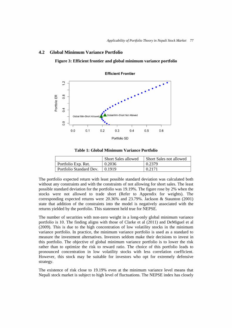
4.2 Global Minimum Variance Portfolio

Figure 3: Efficient frontier and global minimum variance portfolio

Table 1: Global Minimum Variance Portfolio

Short Sales allowed Short Sales not allowed

Portfolio Exp. Ret. 0.2036 0.2379

Portfolio Standard Dev. 0.1919 0.2171

The portfolio expected return with least possible standard deviation was calculated both

without any constraints and with the constraints of not allowing for short sales. The least

possible standard deviation for the portfolio was 19.19%. The figure rose by 2% when the

stocks were not allowed to trade short (Refer to Appendix for weights). The

corresponding expected returns were 20.36% and 23.79%. Jackson & Staunton (2001)

state that addition of the constraints into the model is negatively associated with the

returns yielded by the portfolio. This statement held true for NEPSE.

The number of securities with non-zero weight in a long-only global minimum variance

portfolio is 10. The finding aligns with those of Clarke et al (2011) and DeMiguel et al

(2009). This is due to the high concentration of low volatility stocks in the minimum

variance portfolio. In practice, the minimum variance portfolio is used as a standard to

measure the investment alternatives. Investors seldom make their decisions to invest in

this portfolio. The objective of global minimum variance portfolio is to lower the risk

rather than to optimize the risk to reward ratio. The choice of this portfolio leads to

pronounced concentration in low volatility stocks with less correlation coefficient.

However, this stock may be suitable for investors who opt for extremely defensive

strategy.

The existence of risk close to 19.19% even at the minimum variance level means that

Nepali stock market is subject to high level of fluctuations. The NEPSE index has closely


followed the crests and troughs of political developments in the country, one of the major

reasons for the high fluctuation. But, a 20.36% return even from the least risky portfolio

underlines the high level of business potential in the country.

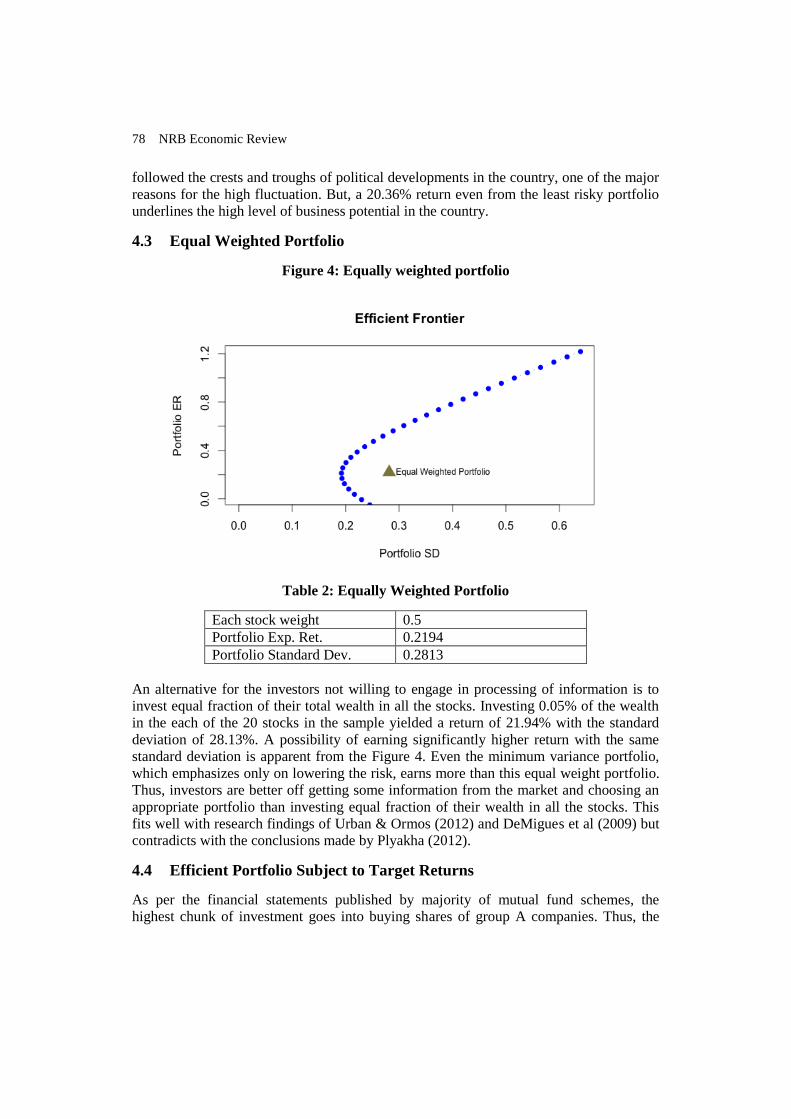
4.3 Equal Weighted Portfolio

Figure 4: Equally weighted portfolio

Table 2: Equally Weighted Portfolio

Each stock weight 0.5

Portfolio Exp. Ret. 0.2194

Portfolio Standard Dev. 0.2813

An alternative for the investors not willing to engage in processing of information is to

invest equal fraction of their total wealth in all the stocks. Investing 0.05% of the wealth

in the each of the 20 stocks in the sample yielded a return of 21.94% with the standard

deviation of 28.13%. A possibility of earning significantly higher return with the same

standard deviation is apparent from the Figure 4. Even the minimum variance portfolio,

which emphasizes only on lowering the risk, earns more than this equal weight portfolio.

Thus, investors are better off getting some information from the market and choosing an

appropriate portfolio than investing equal fraction of their wealth in all the stocks. This

fits well with research findings of Urban & Ormos (2012) and DeMigues et al (2009) but

contradicts with the conclusions made by Plyakha (2012).

4.4 Efficient Portfolio Subject to Target Returns

As per the financial statements published by majority of mutual fund schemes, the

highest chunk of investment goes into buying shares of group A companies. Thus, the


mean-variance model created in this research could be ideal for these mutual funds to

allocate the resources to ensure the attainment of proposed rate of return.

Nabil Investment Banking Limited launched its first mutual fund scheme named Nabil

Balanced fund on March 2013. The scheme is worth 600 millions and has maturity of

five years. The major objective of the scheme is to balance the risk of portfolio by

investing in a mix of securities. The projected Return on Investment (ROI) is 18% and

21% for the third and fourth year. NIBL Capital launched the NIBL Samriddhi Fund – I

with maturity of 7 years on July 2015. The scheme is worth 800 millions and aims at

investing in mixed securities as well. The projected ROI is 19.23% and 24.92% for year 2

and year 3 respectively.

The figure 5 shows the plot of projected return and variation associated with the two

mutual fund companies for the given years. These lie quite close to the minimum

variance portfolio thus the investment needed to produce the stated level of return can be

considered relatively less risky. This indicates the risk averse nature of mutual fund

companies in the country. The other portfolios, preferably higher up the Markowitz bullet

or the tangency portfolio, provide them a better return for the risk they take.

Figure 5: Plot of Returns for Mutual Fund Schemes


Nabil Invest

Figure 6: Nabil Invest Portfolio Weights

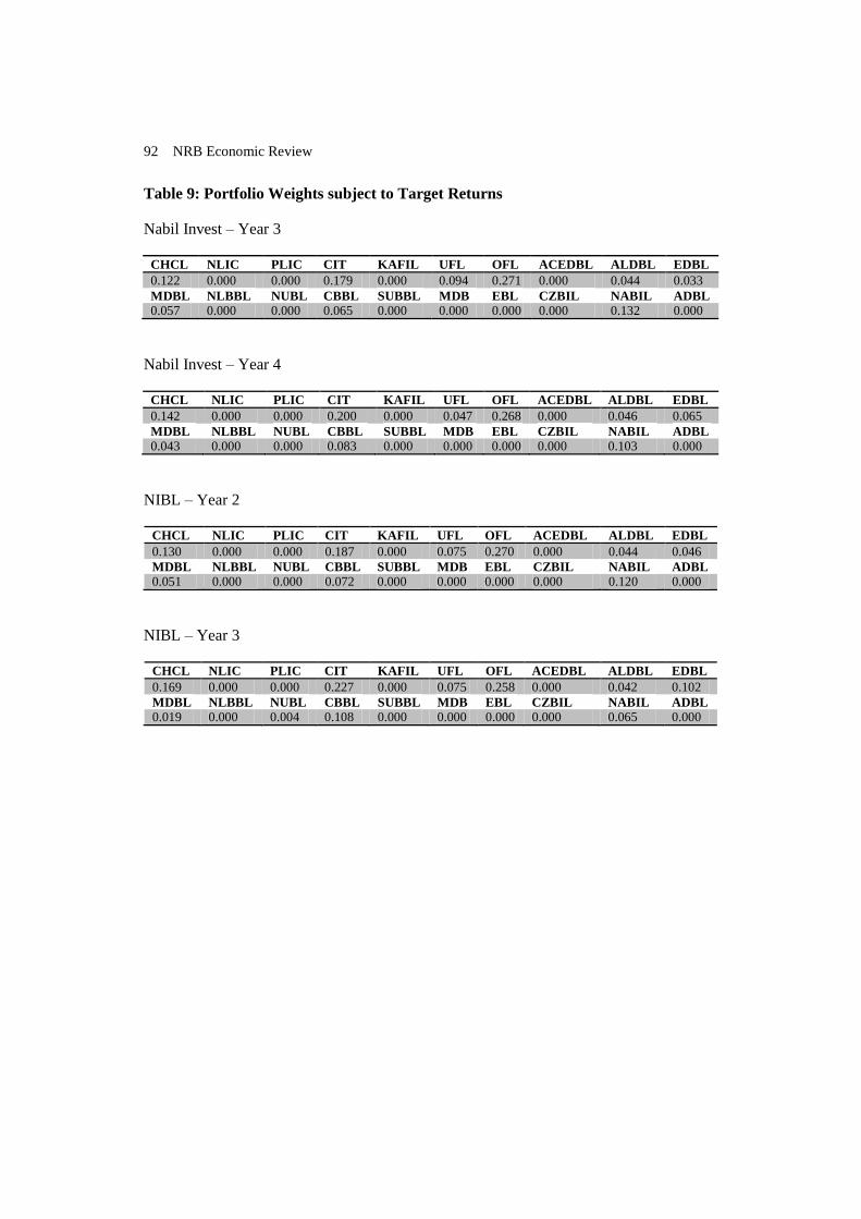
A large part of the return for Nabil Invest in both the third and the fourth year comes from

OFL and CIT stocks. It is worth noting that the low level of risk associated with both

these stocks provides stability to the return earned by the investment of Mutual Fund

Company. This is partly due to the closeness of the returns provided by these mutual fund

schemes to the minimum variance portfolio, and the risk reducing characteristics of these

stocks. The weights for 11 other sample stocks were zero. There is need to change the

weightage during the end of the year, in order to achieve the desired returns. The UFL

and EDBL stocks, in particular, need quite a bit reallocation if the mutual fund is to

provide the stated level of returns to the unit holders.

NIBL Capital

Figure 7: NIBL Capital Portfolio Weights


A large part of return for NIBL comes from OFL, CIT and CHCL stocks. The weights of

10 other stocks are zero for both the years. The UFL stock should be held only for the

year 2 but not for the following year. A fraction of NUBL stock needs to be newly

purchased in the year 3 in order to achieve the return on investment ambitions. The

relative consistency in both the years for OFL stock can be attributed to its less volatility.

The standard deviation of OFL is 40.62%, which is among the lowest for the gives

sample of stocks. The relative consistent level of OFL stock in the portfolio adds stability

to the returns.

From the unit holder‟s perspective, the analysis of minimum variance portfolio and the

returns provided by the mutual funds together provide a point for consideration. The

investment in mutual fund scheme does not seem to be more profitable than looking for

an optimal portfolio to invest on one‟s own. This presents the value of investment related

knowledge to the perspective investors. It is very important for the investors to consider

the stock investment opportunities present in the market and analyze the risk-return

tradeoff, than locking into a modest return proved by a mutual fund.

4.5 Tangency Portfolio

Figure 8: Tangency Portfolio at rf =0.0061

Table 3: Tangency Portfolio at Risk Free Rate 0.61%

Portfolio Exp. Ret. 0.7185

Portfolio Standard Dev. 0.3645

The investors have an option to invest in large universe of risky assets bounded by the

Markowitz bullet. In an economy with lending and borrowing possible at the risk free

rate, an investor can choose to combine the risk free asset with any portfolio on the

frontier. The best portfolio to hold in combination with the risk free rate is the portfolio

yielding highest expected return per unit increase in risk i.e. the one with highest Sharpe

slope, the tangency portfolio. This is the portfolio any investment analyst would suggest

to the client. The choice of allocating the wealth would depend on the risk preference of

the client. Risk averse investors tend to place themselves within the origin and the


tangency portfolio point thus, lending at risk free rate. One the other hand, risk seeking

investors aim to reach a point further away in the line than the tangency portfolio,

borrowing at the risk free rate and investing the proceeds at the tangency portfolio

(Cochrane, 1999; Mayanja, 2011).

The 364-day Treasury bill rate as of August 2015 is 0.61%. The institutional investors

can use this rate as the risk free rate of investment for them. The weights to be allocated

for the tangency portfolio obtained from the model are given in table 4.

Table 4: Tangency Portfolio Weights

CHCL NLIC PLIC CIT KAFIL UFL OFL ACEDBL ALDBL EDBL

0.495 0.348 -0.068 0.329 -0.071 -0.672 0.215 -0.010 0.221 0.350

MDBL NLBBL NUBL CBBL SUBBL MDB EBL CZBIL NABIL ADBL

-0.267 -0.223 0.057 0.288 -0.184 0.259 -0.073 -0.075 -0.145 0.227

A risk averse investor would lie exactly on the y-intercept in figure 8, thus yielding a total

portfolio return equal to the return provided by the treasury bill. If the investor holds

equal of both the treasury bills and the tangency portfolio, a return of 36.23% would be

obtained with a reduction in the portfolio volatility. A risky investor would borrow

money at the rate of Treasury bill and invest proceeds in the tangency portfolio, thus

earning return higher than 71.85%. But, there is a sharp increase in the risk in such

scenario.

4.6 The Applicability Test of Model

The model uses historical performance to obtain estimates of the future characteristics of

the stocks. Fabozzi et al (2002) stated that the performance of developing markets could

be different from the expected performance thus, raising question over the applicability of

the mean variance theory in developing markets like Nepal. Thus, a test check was

necessary to validate the model in case of Nepali stock market.

In order to check the applicability of the model in NEPSE, a test was carried out at the

expected return of 30%. The portfolio weights obtained at the 30% level of returns are

given in table 5.

Table 5: Test Check Weights


0.169 0.021 0.032 0.262 0.000 0.000 0.202 0.000 0.016 0.010


0.00 0.000 0.016 0.143 0.000 0.016 0.000 0.000 0.0171 0.000

A hypothetical wealth of Rs. 100,000 was used to purchase these stocks on December,

2015 market price as per the weights assigned by the model. The weights were divided by

the then share price to come up with the number of each shares to be held. This number

of shares was then multiplied with the market price of the share on April 23, 2014 in

order to come up with the portfolio value.


The portfolio value on April 23, 2014 was Rs. 106,070.68, which amounted to a 110-day

return of 6.06%. This figure was then annualized using,

RA = (1 + 0.0606 )3.3181

– 1

Giving, the annualized return of 21.56%.

The test shows that the mean-variance model was quite close in yielding the desired level

of return for the investor in NEPSE.

The closeness of suggested weight allocation can be calculated using,

100% - ((30 - 21.56) / 30 * 100%)

giving, the closeness figure of 71.86%.

Thus, the model provided 71.86% of the return desired by the investor. This can be

further increased with the increase in accuracy of the parameters being estimated for the

model. Inclusion of real market forces in the model would help the model provide a more

accurate result, as sought by the investor.

V. CONCULSION

This study found that the Markowitz mean-variance method of portfolio analysis is useful

in construction of optimal portfolio from stocks traded at NEPSE. The model provided

71.86% of the desired rate of return by the investors, and has potential to be further

increased with the use of better estimation of return by considering more of the real world

factors. Furthermore, the inclusion of CIT stock in majority of the peculiar-risk-return

portfolios illustrates the importance of active portfolio construction compared to a mere

collection of individual assets. The CIT stock despite having asset specific risk on the

higher side was able to reduce the risk associated with the portfolio due to its negative

correlation coefficient with most of the other stocks present in the portfolio.

The research found a significant lacking of such negatively (or low) correlation stock in

the Nepal stock exchange. Majority of banking stocks, understandably move together

with each other. But the data analysis showed that insurance and hydropower stocks

move in the same trend as the banking stocks do. This has relative disadvantage for the

investors and calls for expansion of the Nepali stock market to encourage the privately

owned companies to enter the market.

The bringing of privately owned real sector companies into the public trading realm

should create a win-win situation for all the stakeholders. The government‟s current

treating of the companies who have gone public on par with the companies who have not

has discouraged the latter to issue public shares, and forced them to remain content with

their current business volume. These privately owned companies should be provided

some tangible benefits in return for their public disclosure of financial position thus,

encouraging their converting to a public company. The existing mechanism of companies

having to float Initial Public Offering only after three years of registering profit and at a

face value of Rs. 100 discourages a profit-making firm. A flexible provision on allowing


the companies to offer their share to public at a premium rate, after an independent

valuation, will definitely encourage their entering the public realm. A mandatory

requirement can be made for companies above a scientifically determined threshold level

of capital to list a certain fraction of their shares for public trading.

The minimum variance portfolio provides return close to 20% and has a similar risk as

well. This sums up the current investment scenario of the country. The high political and

economic risk surrounding the country has translated into significant high minimum level

of risk for the investments. But, the once willing to take on the risk get the reward

through a relatively high level of return. The return provided by the mutual fund is

comparable with the minimum variance portfolio return. This largely means that a

knowledgeable investor able to analyze the market situation should explore the

opportunities present in the stock market than locking the investment in mutual fund

schemes. These schemes seem well suited for elderly and retired people with less ability

or willingness to regularly analyze the investment situations in the market. Tangency

portfolio is the ideal portfolio to consider for every investor and is the one recommended

by portfolio manager to all the investors. There is an immense return of 71.85% for

holding the tangency portfolio. Though the risk associated is quite high, it is largely

compensated by the high return potential, thus the portfolio with highest Sharpe slope.

This research can be a base for additional studies to come. The ability of the model to

come up with asset weights giving the stated rate of return as expected by the investor

seemingly decays over time as the input data and the expected return period get further

and further apart, the characteristic of autoregressive process. This relation could be a

subject of future study through the use of Autoregressive model. The study of portfolio

construction could be widened by consideration of all the scrips available for trading in

NEPSE. With the development of commodities market in Nepal, various commodities,

and financial and non-financial derivatives could be added into the consideration for

construction of an optimal portfolio.

Investors in developing markets like that of Nepal should actively seek more information

rather than following the herd. Investing without an education and research leads to

lamentable investment decision. Research is much more than just listening to the herd.

Phillip Fisher once rightly stated, “The stock market is filled with individuals who know

the price of everything, but the value of nothing.” We would want to do better.

*****


REFERENCES

Amenc, N., F. Goltz, L. Martellini & D. Sahoo. 2011. A Long Horizon Perspective on the Cross-

Sectional Risk-Return Relationship in Equity Markets. EDHEC-Risk Institute Publication.

Ang, A., Hodrick, R., & X. Zhang. 2006. The Cross-section of Volatility and Expected Returns.

Journal of Finance, 61(1), 259-299.

Bali, T., & N. Cakici. 2008. Idiosyncratic Volatility and the Cross Section of Expected Returns.

Journal of Financial and Quantative Analysis, 43(1), 29-58

Cesarone, F., Scozzari, A., & F. Tardella. 2009. Efficient Algorithm for Mean-Variance Portfolio

Optimization with Hard Real-World Constraints. The Magazine Of The Arts, 1–15.

Central Bureau of Statistics. 2004. Nepal living standards survey 2003/04.

Central Bureau of Statistics. 2011. Nepal living standards survey 2010/11.

Clarke, R., De Silva, H. & S. Thorley. 2011. Minimum Variance Portfolio Composition. Journal

of Portfolio Management, 37(2), 31-45.

Cochrane, J. H. 1999. Portfolio advice for a multifactor world. Economic Perspectives. Federal

Reserve Bank of Chicago, 23(3), 59–78.

Cowels, A. 1933. Can Stock Market Forecasters Forecast? Econometrica, 1, 309-324

Dangol, J. 2010. Stock Market Efficiency and Predictability of Prices in Nepal. (Unpublished

M.Phil Research, 2010, Tribhuwan University).

DeMiguel, V., Lorenzo, G. & R. Uppal. 2009. Optimal versus Naive Diversification: How

Inefficient is the 1/N Portfolio Strategy? Review of Financial Studies 22(5), 1915-1953.

Disatnik, D., & S. Katz. 2012. Portfolio Optimization Using a Block Structure for the Covariance

Matrix. Journal of Business Finance & Accounting, 39(5/6), 806–843.

Elton, E. J., & M. J. Gruber. 1974. Portfolio Theory when Investment Relatives are Lognormally

Distributed. Journal of Finance, 29, 1265-1273

Elton, E. J., & M. J. Gruber. 1997. Modern portfolio theory, 1950 to date. Journal of Banking &

Finance, 21(11-12), 1743–1759.

Engels, M. 2004. Portfolio Optimization: Beyond Markowitz. Master’s Thesis, Leiden University.

Retrieved from http://eom.pp.ua/books/[Engels] Portfolio Optimization MSc Thesis

[04].MsuCity.pdf

Fabozzi, F.J., Gupta, F., & H. M. Markowitz, 2002. The Legacy of Modern Portfolio Theory. The

Journal of Investing, 7-22.

Fama, E.F. 1965. The Behavior of Stock-Market Prices. The Journal of Business, 38(1), 34-105.

Fang, Y., Lai, K. K., & S. Y. Wang. 2006. Portfolio rebalancing model with transaction costs

based on fuzzy decision theory. European Journal of Operational Research, 175(2), 879–

893.

Gurung, J. B. 2004. Growth and Performance of Securities Market in Nepal. Journal of Nepalese

Business Studies, 1(1), 85–92.

Golmakani, H. R. & F. Mehrshad. 2011. Constrained Portfolio Selection using Particle Swarm

Optimization. Expert Systems with Applications, 38(7), 8327-8335.


Jagannathan, R. & T. Ma. 2003. Risk Reduction in Large Portfolios: Why Imposing the Wrong

Constraints Helps. Journal of Finance, 58(4), 1651-1684.

Hilsted, J. C. 2012. Active Portfolio Management and Portfolio Construction. (Unpublished

Masters Thesis, 2012, Copenhagen Business School)

Hu, W., & A. N. Kercheval. 2010. Portfolio optimization for student t and skewed t returns.

Quantitative Finance, 10(1), 91–105.

Kraus, A., R. Litzenberger. 1976. Skewness preference and the valuation of risky assets. Journal

of Finance, 21(4), 1085-1100.

Kadariya, S. 2012. Factors affecting investor decision making : A case of Nepalese capital market.

Journal of Research in Economics and International Finance, 1(1), 16–30.

Kaplan, P. D. 1998. Asset Allocation Models Using the Markowitz Approach.

Konno, H., Tanaka, K., & R. Yamamoto. 2011. Construction of a portfolio with shorter downside

tail and longer upside tail. Computational Optimization and Applications, 48(2), 199–212.

Konno, H., & H. Yamazaki. 1991. Mean-Absolute Deviation Portfolio Optimization Model and Its

Applications to Tokyo Stock Market. Management Science, 37(5), 519–531.

Lintner, J. 1965. The Valuation of Risk Assets and the Selection of Risky Investments in Stock

Portfolios and Capital Budgets. Review of Economics and Statistics, 47, 13-37.

Lai, T. L., Xing, H., & Z. Chen. 2011. Mean-variance portfolio optimization when means and

covariances are unknown. Annals of Applied Statistics, 5(2 A), 798–823.

Maillard,S. , Roncalli, T. & J. Teiletche. 2010. On the Properties of Equally-Weighted Risk

Contributions Portfolios. Journal of Portfolio Management, 36(4), 60-70.

Markowitz, H. M. 1952. Portfolio Selection. The Journal of Finance, 7(1), 77–91.

Markowitz, H. M. 1999. The History of Portfolio Theory : Portfolio Theory : 1600 - 1960.

Financial Analysts Journal, 55(4), 5–16.

Markowitz, H. M., & Dijk, E. L. Van. 2014. Single-Period in a Mean-Variance Analysis Changing

World. Financial Analysts Journal, 59(2), 30–44.

Markowitz, H. M., Lacey, R., Plymen, J., Dempster, M. a. H., & R.G. Tompkins. 1994. The

General Mean-Variance Portfolio Selection Problem. Philosophical Transactions of the

Royal Society A: Mathematical, Physical and Engineering Sciences, 347(1684), 543–549.

Mayanja, F. 2011. Portfolio Optimization Model: The Case of Uganda Securities Exchange.

University of Dar es Salaam.

Mokta, R. S. 2013. Optimal Portfolio Construction: Evidence from Dhaka Stock Exchange in

Bangladesh. World Journal of Social Sciences, 3(6), 75-87.

Mokhtar, M., Shuib, A., & D. Mohamad. 2014. Mathematical Programming Models for Portfolio

Optimization Problem : A Review. International Journal of Social, Education, Economics

and management Engineering, 8(2), 428–435.

Mossin, J. 1966, Equilibrium in a Capital Asset Market, Econometrica, 34, 468-483.

Paudel, D. R. B., & S. Koirala. 2007. Application of Markowitz and Sharpe Models in Nepalese

Stock. Journal of Nepalese Business Studies, 3(1), 18–35.


Paudel, N. P. 2002. Investing in Shares of Commercial Banks in Nepal : an Assessment of Return

and Risk Elements. Economic Review: Occasional Paper, 14.

Plyakha, Y., Uppal, R., & G. Vilkov. 2012. Why Does an Equal-Weighted Portfolio Outperform

Value-and Price-Weighted Portfolios? SSRN 1787045.

Puelz, A. V. 2002. A Stochastic Convergence Model for Portfolio Selection. Operations Research,

50(3), 462-476.

Maillard, S., Roncalli, T., & J. Teiletche. 2010. On the properties of equally-weighted. Working

Paper, 1–23.

Roncalli, T., & L. A. Management. 2010. Understanding the Impact of Weights Constraints in

Portfolio Theory, Lyxor Asset Management.

Soleiman, H. , Golmakani, H. R., & M. H. Salimi. 2009. Markowitz-based Portfolio Selection with

Minimum Transaction Lots, Cardinality Constraints and Regarding Sector Capitalization

using Genetic Algorithm. Expert Systems with Applications, 36(3), 5058-5063.

Sharpe, W. F. 1964. Capital Asset Prices: A Theory of Market Equilibrium under Conditions of

Risk. Journal of Finance, 19(3), 425-442.

Taghizadegan, G. , Darvish, Z. A. & A. Y. Bakhshayesh. 2014. Portfolio Optimization of Equity

Mutual Funds in Tehran Stock Exchange (TSE) with Fuzzy Set. Management and

Administrative Sciences Review, 3(4), 484-494.

Tobin, J. 1981. Portfolio theory. Science (New York, N.Y.), 214(4524).

Urbán, A., & M. Ormos. 2012. Performance analysis of equally weighted portfolios: USA and

Hungary. Acta Polytechnica Hungarica, 9(2), 155–168.

Williams, J. B. 1938. The Theory of Investment Value. Cambridge, MA: Harvard University

Press.


Appendices

A. Stocks Used in the Sample & their Abbreviations

Commercial Banks (4)

Agriculture Development Bank (ADBL)

Everest Bank Limited (EBL)

Citizens Bank Limited (CZBIL)

Nabil Bank (NABIL)

Finance Companies (4)

Kaski Finance Company (KAFIL)

United Finance Company (UFL)

Om Finance Limited (OFL)

Citizen Investment Trust (CIT)

Insurance Companies (2)

Prime Life Insurance Company (PLIC)

Nepal Life Insurance Company (NLIC)

Development Banks (9)

Ace Development Bank (ACEDBL)

Alpine Development Bank (ALDBL)

Excel Development Bank (EDBL)

Malika Bikas Bank (MDBL)

Nerude Laghubitta Bikas Bank (NLBBL)

Nirdhan Utthan Bank (NUBL)

Subechha Bikas Bank (SUBBL)

Miteri Development Bank (MDB)

Chhimek Laghu Bitta Bikas Bank (CBBL)

Others (1)

Chilime Hydropower Company (CHCL)

B. Portfolio Characteristics

Table 6: Expected Annual Return


0.227 0.440 0.417 0.442 0.101 -0.040 0.060 0.116 0.132 0.293


0.041 0.304 0.389 0.457 -0.002 0.272 0.182 0.172 0.094 0.286

Table 7: Covariance Matrix

CHCL NLIC PLIC CIT KAFIL UFL OFL ACEDBL ALDBL EDBL MDBL NLBBL NUBL CBBL SUBBL MDB ADBL EBL CZBIL NABIL

CHCL 0.187

NLIC 0.050 0.258

PLIC 0.127 0.094 0.232

CIT -0.005 0.076 -0.005 0.243

KAFIL 0.079 0.094 0.106 -0.035 0.262

UFL 0.029 0.082 0.020 0.009 0.053 0.178

OFL -0.013 0.049 0.024 -0.007 0.063 0.074 0.165

ACEDBL 0.124 0.051 0.123 -0.023 0.139 0.068 0.007 0.227

ALDBL 0.042 0.028 0.054 -0.019 0.132 0.091 0.061 0.103 0.172

EDBL 0.030 0.081 0.062 0.040 0.057 0.097 0.000 0.103 0.064 0.208

MDBL 0.082 0.066 0.044 -0.016 0.113 0.097 0.040 0.120 0.082 0.087 0.173

NLBBL 0.099 0.066 0.110 -0.006 0.126 0.038 0.060 0.084 0.092 0.037 0.035 0.304

NUBL 0.014 0.074 0.073 0.040 0.049 0.094 0.039 0.081 0.097 0.102 0.050 0.067 0.227

CBBL 0.053 -0.017 0.072 -0.069 0.073 0.023 0.034 0.070 0.086 0.030 0.035 0.166 0.083 0.351

SUBBL 0.077 0.072 0.042 0.015 0.100 0.105 0.050 0.103 0.097 0.088 0.109 0.050 0.042 0.043 0.277

MDB 0.034 0.065 0.026 -0.043 0.092 0.156 0.100 0.082 0.118 0.079 0.134 0.091 0.103 0.097 0.124 0.394

ADBL 0.094 0.095 0.121 0.005 0.099 0.081 0.034 0.081 0.078 0.082 0.100 0.090 0.067 0.042 0.079 0.100 0.194

EBL 0.132 0.089 0.103 0.010 0.111 0.062 0.003 0.118 0.059 0.065 0.104 0.073 0.048 0.027 0.075 0.073 0.138 0.184

CZBIL 0.134 0.124 0.111 0.007 0.143 0.110 0.069 0.164 0.097 0.091 0.133 0.101 0.052 0.066 0.127 0.124 0.132 0.166 0.309

NABIL 0.117 0.078 0.119 0.013 0.113 0.019 -0.011 0.127 0.036 0.062 0.071 0.093 0.020 0.021 0.061 0.010 0.112 0.152 0.154 0.215


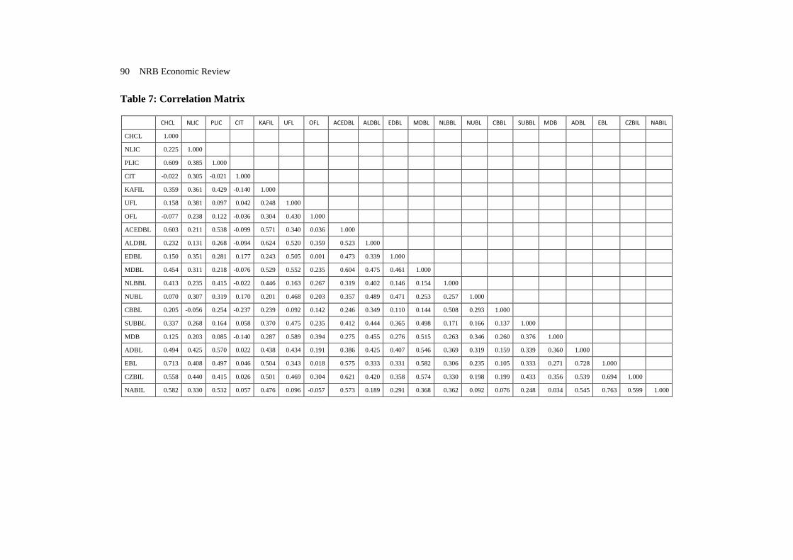
Table 7: Correlation Matrix

CHCL NLIC PLIC CIT KAFIL UFL OFL ACEDBL ALDBL EDBL MDBL NLBBL NUBL CBBL SUBBL MDB ADBL EBL CZBIL NABIL

CHCL 1.000

NLIC 0.225 1.000

PLIC 0.609 0.385 1.000

CIT -0.022 0.305 -0.021 1.000

KAFIL 0.359 0.361 0.429 -0.140 1.000

UFL 0.158 0.381 0.097 0.042 0.248 1.000

OFL -0.077 0.238 0.122 -0.036 0.304 0.430 1.000

ACEDBL 0.603 0.211 0.538 -0.099 0.571 0.340 0.036 1.000

ALDBL 0.232 0.131 0.268 -0.094 0.624 0.520 0.359 0.523 1.000

EDBL 0.150 0.351 0.281 0.177 0.243 0.505 0.001 0.473 0.339 1.000

MDBL 0.454 0.311 0.218 -0.076 0.529 0.552 0.235 0.604 0.475 0.461 1.000

NLBBL 0.413 0.235 0.415 -0.022 0.446 0.163 0.267 0.319 0.402 0.146 0.154 1.000

NUBL 0.070 0.307 0.319 0.170 0.201 0.468 0.203 0.357 0.489 0.471 0.253 0.257 1.000

CBBL 0.205 -0.056 0.254 -0.237 0.239 0.092 0.142 0.246 0.349 0.110 0.144 0.508 0.293 1.000

SUBBL 0.337 0.268 0.164 0.058 0.370 0.475 0.235 0.412 0.444 0.365 0.498 0.171 0.166 0.137 1.000

MDB 0.125 0.203 0.085 -0.140 0.287 0.589 0.394 0.275 0.455 0.276 0.515 0.263 0.346 0.260 0.376 1.000

ADBL 0.494 0.425 0.570 0.022 0.438 0.434 0.191 0.386 0.425 0.407 0.546 0.369 0.319 0.159 0.339 0.360 1.000

EBL 0.713 0.408 0.497 0.046 0.504 0.343 0.018 0.575 0.333 0.331 0.582 0.306 0.235 0.105 0.333 0.271 0.728 1.000

CZBIL 0.558 0.440 0.415 0.026 0.501 0.469 0.304 0.621 0.420 0.358 0.574 0.330 0.198 0.199 0.433 0.356 0.539 0.694 1.000

NABIL 0.582 0.330 0.532 0.057 0.476 0.096 -0.057 0.573 0.189 0.291 0.368 0.362 0.092 0.076 0.248 0.034 0.545 0.763 0.599 1.000

Table 8: Global Minimum Variance Portfolio

8.1: With Short selling allowed

Portfolio expected return: 0.203

Portfolio standard deviation: 0.191

Portfolio weights:


0.324 0.055 -0.079 0.182 -0.012 0.043 0.345 0.006 0.134 0.132


0.009 -0.131 -0.038 0.142 -0.060 0.0182 -0.030 -0.245 0.236 -0.022

8.2: Not allowing for short sales

Portfolio expected return: 0.237

Portfolio standard deviation: 0.217

Portfolio weights:


0.165 0.000 0.000 0.219 0.000 0.003 0.266 0.000 0.047 0.095


0.030 0.000 0.000 0.099 0.000 0.000 0.000 0.000 0.076 0.000


Table 9: Portfolio Weights subject to Target Returns

Nabil Invest – Year 3


0.122 0.000 0.000 0.179 0.000 0.094 0.271 0.000 0.044 0.033


0.057 0.000 0.000 0.065 0.000 0.000 0.000 0.000 0.132 0.000

Nabil Invest – Year 4


0.142 0.000 0.000 0.200 0.000 0.047 0.268 0.000 0.046 0.065


0.043 0.000 0.000 0.083 0.000 0.000 0.000 0.000 0.103 0.000

NIBL – Year 2


0.130 0.000 0.000 0.187 0.000 0.075 0.270 0.000 0.044 0.046


0.051 0.000 0.000 0.072 0.000 0.000 0.000 0.000 0.120 0.000

NIBL – Year 3


0.169 0.000 0.000 0.227 0.000 0.075 0.258 0.000 0.042 0.102


0.019 0.000 0.004 0.108 0.000 0.000 0.000 0.000 0.065 0.000

GUIDELINES FOR ARTICLE SUBMISSION

NRB Economic Review, previously published as the "Economic Review Occasional

Paper", is a bi-annual peer-reviewed economic journal being published in April and

October. Submission of a paper for the NRB Economic Review will be taken to imply that

it represents original work not previously published, and it is not being considered

elsewhere for publication, and that if accepted for publication it will not be published

anywhere without the consent of the Editorial Board. The papers so received have to

undergo a double blind review process and are then subject to approval by the Editorial

Board. However, the ideas and opinions expressed in the papers published in the Review

are solely those of authors and in no way represent views and policies of Nepal Rastra

Bank or that of the Editorial Board.

Submitted manuscripts should be written in English, typed in double spacing with wide

margins (3 cm) on one side of standard paper. The title page should contain the title, the

name, institutional affiliation(s), JEL classification, key words, full postal address,

telephone/fax number and E-mail of each author, and, in the case of co-authorship

indicate the corresponding author. In case the author(s) is provided grant or any type of

financial support from any organization or institution, this should be spelled out clearly

below the key words. Footnotes, if any, should be numbered consecutively with

superscript arithmetic numerals at the foot of each page. Figures and tables should be on

separate sheets and have descriptive titles. References in the text should follow the

author-date format. References should be listed alphabetically in the following style:

Anderson, T. W. and C. Hsiao. 1982. "Formulation and Estimation of Dynamic Models

Using Panel Data." Journal of Econometrics 18: 47–82.

Goldstrein, M. and M. Khan. 1985. "Income and Price Effects in Foreign Trade." In R.

W. Joners and P. B. Kenen, eds., Handbook of International Economics, vol. II,

Elsevier, New York.

Hemphill, W. 1974. "The Effect of Foreign Exchange Receipts on Imports of Less

Developed Countries." IMF Staff Papers 21: 637–77.

The manuscript should be accompanied by an abstract not exceeding 300 words, and the

preferred maximum length of a submission is 10,000 words. The preferred word

processing software for the Review is Microsoft Word. Authors should e-mail their

manuscript to:

The Editorial Board

NRB Economic Review

Nepal Rastra Bank

Research Department

Baluwatar, Kathmandu


Telephone: 977-1-4419804, Ext. 265

Past Issues of NRB Economic Review are available at www.nrb.org.np under Publication

NRB ECONOMIC REVIEW ISSN 1608-6627

Nepal Rastra Bank Central Office, Research Department

Baluwatar Kathmandu, Nepal

Phone: 977-1-4411638

Fax: 977-1-4441048


Website: www.nrb.org.np

applicability of portfolio theory in nepali stock market

Documents