APPENDIX A

ELEVATION ANGLE DEPENDENCE FOR SLANT PATH COMMUNICATIONS LINKS

Very often in radiowave propagation calculations it is necessary to evaluate a path length dependent parameter, such as atmospheric attenuation, path delay, or rain attenuation, as a function of the elevation angle () of the ground antenna to the satellite. Atmospheric attenuation models are usually developed for the zenith «() = 90°) direction, and attenuation at other elevation angles must be derived from that value. Rain attenuation modeling, on the other hand, is most often developed for terrestrial paths «() = 0°) and other values of attenuation for slant paths must be derived from it.

In this appendix the general procedure for determining elevation angle de­pendence for a slant path is developed.

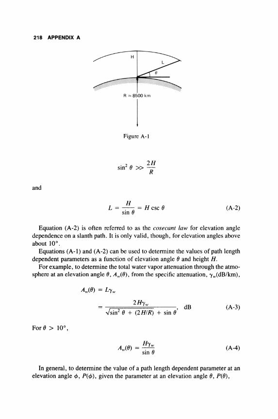
Consider a horizontally stratified interaction region in the atmosphere of height H above the surface of the spherical earth with an effective radius (in­cluding refraction) of R, as shown in Figure A-I. We desire to determine the path length L through the stratified atmosphere, as a function of the elevation angle (). The value for R is usually taken as 8500 km. H will typically range up to 10-20 km maximum for most parameters of interest for radiowave propa­gation factors.

The path length L is then found from geometric considerations as

2H L = -;==;0=====----

.Jsin2 () + (2HIR) + sin () (A-i)

This result is valid for all elevation angles from () = 0°, where L = .J2RH, to () = 900, where L = H, under the reasonable assumption that R » 2 H.

A further simplification is possible for elevation angles greater than about 10°. For () between 10° and 90°, sin2 () will range between 0.03 and 1. The maximum value of 2HIR will be on the order of 0.0024 forthe values discussed above. Therefore for () > 10°,

217

218 APPENDIX A

and

R "" 8500km

Figure A-I

2H sin2 (J » Ii

H L = -- = H csc (J

sin (J (A-2)

Equation (A-2) is often referred to as the cosecant law for elevation angle dependence on a slanth path. It is only valid, though, for elevation angles above about 10°.

Equations (A-I) and (A-2) can be used to determine the values of path length dependent parameters as a function of elevation angle (J and height H.

For example, to determine the total water vapor attenuation through the atmo­sphere at an elevation angle (J, Aw((J), from the specific attenuation, 'Yw(dB/km),

2H'Yw dB ../sin2 (J + (2H1R) + sin (J'

(A-3)

(A-4)

In general, to determine the value of a path length dependent parameter at an elevation angle cf>, P( cf», given the parameter at an elevation angle (J, P( (J),

ELEVATION ANGLE DEPENDENCE 219

or

Then,

PC</»~ = P«()) L(</» L«())

PC</»~ = L(</» P«()) L«())

.J sin2 () + (2 HI R) + sin () PC</»~ = P«())

.Jsin2 </> + (2H1R) + sin </>

If both () and </> are greater than 10°,

sin () PC</»~ = -. - P«())

SIn </>

(A-5)

(A-6)

These results are used in the developments of gaseous attenuation (Chapter 3), rain, cloud and fog attenuation (Chapter 4), and in several other sections throughout the text.

APPENDIX B

INTERPOLATION PROCEDURE FOR ATMOSPHERIC ATTENUATION

COEFFICIENTS

Tables 3-1 and 3-2 present listings of frequency dependent coefficients for use in the detennination of specific attenuation and total zenith attenuation due to gaseous atmospheric absorption. To detennine the coefficients at frequencies other than those given in the tables, the following procedure should be used.

Given the frequency/coefficient pairsfl/YI andf2/Y2, from either table, where Y is a(/), b(/), c(/), or a(/), (3(/), Hf), we desire to detennine the coeffi­cient Yo at frequency fo (see Figure B-1).

Note that,

log Y2 = m logf2 + b ' (B-1)

and

log YI = m logfl + b ' (B-2)

Solving for m and b I,

log [(yh2)] m=

log [(Nf2)] (B-3)

b ' = log Y2 - m logf2 (B-4)

The coefficient Yo at frequency fo is then found from

log Yo = m logfo + b ' (B-5)

where m and b ' are detennined from Equations (B-3) and (B-4) above. For example, to detennine the (3(/) coefficient at 17.5 GHz from Table 3-2,

220

f­Z w U LL LL W o u

ATMOSPHERIC ATTENUATION COEFFICIENTS 221

y2r-----------------------~

y 1 t--------7!"

f 0

FREQUENCY

WHERE. f: FREQUENCY IN GHz y: a(fl. b(fl. AND e(fl

IN TABLE (3-11 OR

a(fl. Il(fl. AND WI IN TABLE (3-21

Figure 8-1

II = 16 GHz

12 = 20 GHz

lu = 17.5 GHz

(31(f) = 0.00821

(32U) = 0.0346

(3oU) = ???

From Equation (B-3),

log [(0.0082110.0346)] m = = 6.447

log [(16/20)]

From Equation (B-4),

b ' = log 0.0346 - 6.447 log 20

= -9.848

Therefore, from Equation (B-5),

log (3oU) = 6.447 log 17.5 - 9.848 = -1.8341

(3oU) = 0.01465

The aU) and Hf) coefficients for 17.5 GHz can be found in a similar man­ner.

APPENDIX C

ANALYTICAL BASIS FOR THE aRb REPRESENTATION OF RAIN

ATTENUATION

The specific attenuation produced by rain on a radiowave path was found in Chapter 4 to be well approximated by the expression

(C-l)

where R is the rain rate in mm/h and a and b are frequency and temperature dependent constants. In this appendix the analytical basis for this relationship is developed from the classical descriptions of rain attenuation on a radiowave path.

Consider the specific attenuation in terms of the attenuation cross-section Qt and drop size distribution n(r), as given by Equation (4-13)

(C-2)

where [see Eq. (4-12)]

In these equations Qt is the attenuation cross section, r is the rain drop diameter, A is the wavelength, m is the refractive index of the water drop, R is the rain rate in mm/h, and No, c, and d are empirical constants.

The attenuation cross section is given by [see Equation (4-9)]

(C-3)

222

THE aFr> REPRESENTATION OF RAIN ATTENUATION 223

In the region where 27r r « }.., i.e., where the Rayleigh Scattering condition applies,

or

Only the first term of b l is signfiicant compared to the other terms, therefore

}..2 Q = - 3 Re b '27r I

(C-4)

where Re indicates "the real part of," and 1m "the imaginary part of." Then, substituting Q, from Equations (C-4) into Equation (C-2)

0' = 4.343No 87r2 [1m m: - q [000

r3 e- Ar dr (C-5) }.. L m- + 2J J

Evaluating the definite integral,

(C-6)

For typical values of rain rate R and drop size r, with the Marshall-Palmer drop size distribution assumed, the second term in the integral will be negligible compared to the first term, as shown by Table C-I.

The integral therefore reduces to the value 61 A 4 , and Equation (C-5) becomes

0'=

or

0' = a~ (C-7)

224 APPENDIX C

R (mm/hr)

.25

10

25

50

100

200

where

and

Table C-1. Comparison of Terms in Integral

r3 e-fl.r dr = - - - r3 e-fl.r ~ oo 6 1

o A4 A t t

Term 1 Term 2

A = 820R-·21 (Marshall-Palmer Distribution)

r (mm)

0.25 0.75 1.25

0.25 0.75 1.25

0.25 0.75 1.25

0.25 0.75 1.25

0.25 0.75 1.25

0.25 0.75 1.25

0.25 0.75 1.25

Tenn 1

2.28 x 10- 2

7.31 x 10- 2

0.566

1.09

1.96

3.50

6.27

m2 - 1 4.343N04811'2 1m -=-2-­

m + 2 a = ------~-----

AC4

b = 4d

Tenn 2

1.74 X 10- 16

7.08 x 10-39

4.9 x 10-62

2.38 X 10- 13

1.00 .( 10-29

7.27 x 10-47

1.01 x 10-9

2.84 x 10- 19

1.37 x 10- 29

1.11 x 10-8

2.62 x 10- 16

1.06 x 10-24

5.27 x 10- 8

2.10 x 10- 19

1.43 x 10- 21

2.066 x 10-7

9.48 x 10- 13

7.45 x 10- 19

6.87 x 10- 7

2.6 x 10- 11

1.69 x 10- 16

(C-8)

(C-9)

APPENDIX D

CRANE GLOBAL RAIN ATTENUATION MODEL CALCULATION PROCEDURE

This appendix presents the step-by-step procedure for the calculation of rain attenuation for an average year by use of the Crane global model, discussed in Chapter 5, Section 5.4.

The input parameters required for the Crane Global Model are:

f Frequency (GHz) 8: Elevation angle to satellite (degrees) G: Ground station elevation, i.e., the height above mean sea level (km) ¢: Ground station latitude (degrees)

The mean rain attenuation distribution for an average year is determined as follows:

STEP 1. Obtain the annual rain rate distribution, Rp, for values of p from 2 % to 0.001 % of an average year, for the location of interest. If this information is not available from local historical data sources, use the appropriate rain rate distribution listed in Table 4-9, as determined from the climate regions given by the maps of Figures 4-8, 4-9, or 4-10.

STEP 2. Determine the O°C isotherm height H(p) for each percent of the average year p from Figure 4-11. Isotherm heights for p = 0.00 1 %, 0.01 % , 0.1 %, and 1 % can be read directly off of the curves on the figure. Isotherm heights at other values of p can be determined by logarithmic interpolation be­tween the curves.

STEP 3. Calculate the projected surface path length D for each p percent of the year desired from the following:

For 8 ~ 100,

D = H(p) - G tan 8

(D-1)

where H(p) are the 0 0 isotherm heights obtained in Step 2, G is the ground

225

226 APPENDIX D

station elevation above mean sea level, and () is the elevation angle to the sat­ellite.

At elevation angles less than 10°, the curvature of the earth's surface must be accounted for. Therefore, for () < 10°,

D = R sin-I

J cos () (.J(G + R)2 sin2 () + 2R(H(p) - G) + H2(p) - G 2

LH(p) + R

- (G + R) sin ()) J (D-2)

where R is the effective radius of the earth, assumed to be 8500 kIn. STEP 4. Determine the specific attenuation coefficients a and b at the fre­

quency and polarization of interest. The values given by Table 4-3 are recom­mended.

STEP 5. Determine the following four empirical constants from Rp for each p of interest.

d = 3.8 - 0.6 In Rp (D-3)

x = 2.3R;;o.17 (D-4)

y = 0.026 - 0.03 In Rp (D-5)

(D-6)

STEP 6. The mean slant-path rain attenuation at each probability of occur­rence p is then found as follows:

(a) If 0 < D ::5 d:

(b) If d < D ::5 22.5:

aft.. r eUbD - IJ A(p) = ~ cos () Ub

aft.. reUbd - 1 _ xeYbd + Xb eYbDJ A(p) = -=.L

cos () Ub Yb Yb

(D-7)

(D-8)

CRANE GLOBAL RAIN ATTENUATION MODEL CALCULATION PROCEDURE 227

(c) If D > 22.5, calculate A(p) with D = 22.5 but use the rain rate R; at the value

l22.5l p'=p -D

(D-9)

instead of Rp-STEP 7. Estimate the upper and lower bounds of the mean slant-path atten­

uation (i.e., the standard deviation of measurements about the model) from the following:

Percent Standard of Year Deviation (%)

1.0 ±39 0.1 32 0.01 32 0.001 39

For example, a mean prediction of 12 dB at 0.01 % of the year yields an upper! lower bound of ±32% or ±3.84 dB.

APPENDIX E

CCIR RAIN ATTENUATION MODEL CALCULATION PROCEDURE

This appendix presents step-by-step procedures for the calculation of rain at­tenuation for an average year by application of the CCIR rain attenuation model discussed in Chapter 5, Section 5.5. Three separate methods are included in the CCIR model:

Method I: for maritime climates Method II: for continental climates and/or for time percentages greater than

0.01 % Method I': for tropical climates

The CCIR Model determines an annual attenuation distribution at a specified location from as "average year" rain rate distribution. The input parameters required for the model are:

f: frequency (GHz) (): elevation angle to the satellite (degrees) G: Ground station elevation, i.e., the height above mean sea level (km) cJ>: Ground station latitude (degrees)

The step-by-step procedure for each method follows.

METHOD I. MARITIME CLIMATES

STEP 1. Obtain the rain height hR from

hR = 5.1 - 2.15 log [1 + 10(<1>-27/25)] (E-l)

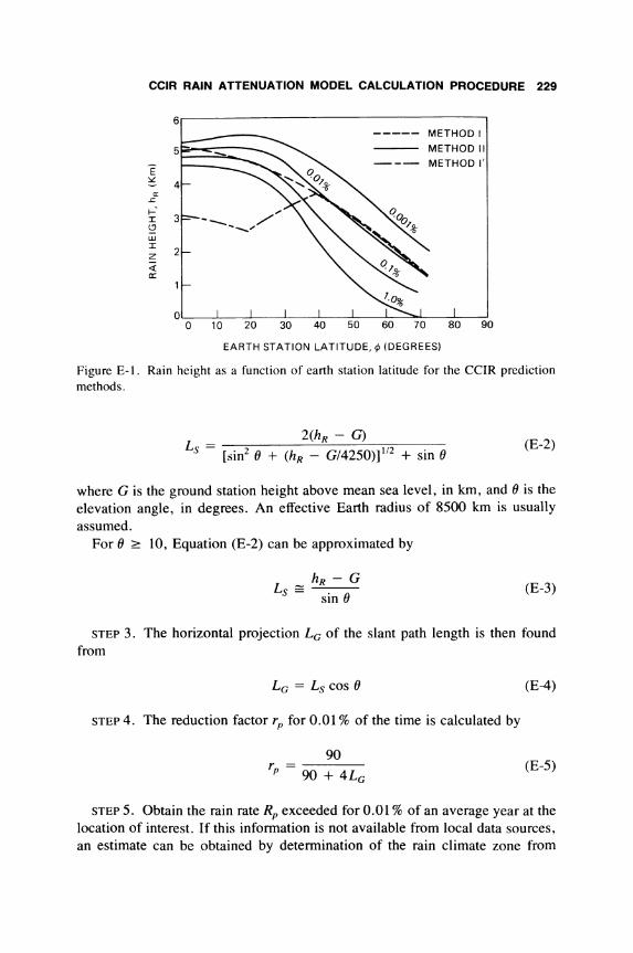
where cJ> is the ground station latitude, in degrees. This equation is shown plot­ted in Figure E-l as the curve labeled "Method I."

STEP 2. The slant path length Ls is determined from

228

CCIR RAIN ATTENUATION MODEL CALCULATION PROCEDURE 229

6 ----- METHOD I

5

E ~

4 a:

-'" ... ' 3 I

'=" UJ I

2 z ;;{ 0::

OL-__ ~ __ -L __ ~ __ ~ ____ L-__ ~~w-__ -L __ -J

o 10 30 40 90

EARTH STATION LATITUDE, ¢ (DEGREES)

Figure E-J. Rain height as a function of earth station latitude for the CCIR prediction methods.

Ls = [sin2 fJ + (hR - G/4250)] 1/2 + sin fJ (E-2)

where G is the ground station height above mean sea level, in km, and fJ is the elevation angle, in degrees, An effective Earth radius of 8500 krn is usually assumed.

For fJ ~ 10, Equation (E-2) can be approximated by

hR - G Ls == sin fJ

(E-3)

STEP 3. The horizontal projection Lc of the slant path length is then found from

Lc = Ls cos fJ (E-4)

STEP 4, The reduction factor rp for 0.01 % of the time is calculated by

90 r = -------p 90 + 4Lc

(E-5)

STEP 5. Obtain the rain rate Rp exceeded for 0.01 % of an average year at the location of interest. If this information is not available from local data sources, an estimate can be obtained by determination of the rain climate zone from

230 APPENDIX E

Figures 4-13 or 4-14, and the corresponding rain rate value at 0.01 % from Table 4-10.

STEP 6. Obtain the specific attenuation ex from

ex = aR!, dB/kIn (E-6)

where a and b are the frequency dependent constants described by Equation (4-15). The values given by Table 4-3 are recommended.

STEP 7. The rain attenuation exceeded for 0.01 % of the average year is then obtained from

(E-7)

STEP 8. The rain attenuation for other percentages p of the average year is found from Equation (E-7) by

A = p

( )-0.33

Ao.oI 0~1 '

( )-0.41

Ao.ol 0~1 '

0.001 !5; p !5; 0.01

0.01 < P !5; 0.1

METHOD II. CONTINENTAL CLIMATES

(E-8)

Method II is used for locations in continental climates and/or when time per­centages greater than 0.1 % are required. It is somewhat more invovled than is Method I, since it uses four rain rate distribution values rather than the single value at 0.01 % used in Method I.

STEP 1. Obtain the rain height hR for the four percentage values 0.001 %, 0.01 %, 0.1 %, and 1 % at the ground location of interest from the curves of Figure E-l labeled "Method II."

STEP 2. Determine the slant-path length Ls from Equations (E-2) or (E-3), as in Method I, Step 2.

STEP 3. Determine the horizontal projection LG from Equation (E-4) as in Method I, Step 3.

STEP 4. The reduction factor rp is determined for each of the four time per­centages from

10 (E-9) ro.OOI = ---

10 + LG

CCIR RAIN ATTENUATION MODEL CALCULATION PROCEDURE 231

90 rO.OI

90 + 4LG (E-1O)

180 rO.1

180 + LG (E-ll)

rl.o = (E-12)

STEP 5. Obtain the rain rate Rp at the location of interest exceeded for 0.001 %, 0.01 %, 0.1 %, and 1.0% of an average year. If this infonnation is not available from local data sources, use the appropriate rain rate distribution listed in Table 4-9, as detennined from the climate regions given by the maps of Figures 4-8,4-9, or 4-10.

STEP 6. The rain attenuation exceeded for each of the four time percentages is found from

AO.OOI = aRg.oolLsro.oo I (E-13)

Ao.ol = am.ol Lsro.ol (E-14)

AO.I = aRg.ILsrol (E-15)

AI = aK;Lsrl (E-16)

where a and b are the frequency dependent constants for specific attenuation described by Equation (4-15).

STEP 7. The rain attenuation for other percentages p between 0.001 % and 1. 0 % is found from Equations (E-13) through (E-16) by the following

A = p

A (_p_)IOg[(AO.OO1/AO.OI)]

0.001 0.001 '

A (~)IOg[(AO.OI/Ao.OI)]

0.01 0.01 '

(x..)IOg[(AO.'/AI»)

AO.I 0.1 '

METHOD I'. TROPICAL CLIMATES

0.001 < P < 0.01

0.01 < P < 0.1

0.1 < P < 1

(E-17)

Method I was modified by the CCIR IWP 5/2 in May 1982 to improve the prediction for tropical climates where the original Method I was found to overpredict the rain attenuation.

232 APPENDIX E

The Method I' procedure differs from Method I in two ways. First, the rain height hR calculated in Step I, Equation (E-l), is modified by a reduction factor Pp which is a function of ground station latitude. The modified rain height hR is found from

where

{0.6,

Pp = 0.6 + 0.02(ct> - 20),

1.0,

(E-18)

(E-19)

The modified rain height is shown plotted in Figure E-1 as the curve labeled "Method I'."

Method I Steps 2 through 7 are unchanged for Method I'. The second modification occurs in Step 8, the calculation of rain attenuation

for other percentages of the year. Method I' includes an additional equation for calculating rain attenuation for percentages from 0.1 to 1.0%. Equation (E-8) is extended to

A = p

( )~O.33

Ao.oJ 0~1 '

( )~O.9J

Ao.oJ 0~1 '

( )~O.5

1.3Ao.oJ 0~1 '

0.001 :5 P :5 0.01

0.01 < P :5 0.1 (E-20)

0.1 < P :5 1

Method I' provides predictions which are identical to Method I for locations above 40° latitude, and provides predictions which are reduced by up to about 40% for locations below 20° latitude.

Method I' was adapted by CCIR Study Group V at it's 1983 Interim Meetings in Geneva as the sole CCIR Prediction Model to be used for attenuation pre­diction calculations (CCIR Doc. 5/101, 27 July 1983).

APPENDIX F

CCIR TROPOSPHERIC SCINTILLATION MODEL PROCEDURE

In this appendix the detailed step by step procedure of the CCIR tropospheric scintillation model introduced in Chapter 8 is presented. A thin turbulent layer at an average height of 1 km is assumed, and empirical approximations to the determination of amplitude fluctuations from turbulence theory are employed in the model.

The model determines the standard deviation of the log of the received power, which is a measure of the root mean square (r.m.s.) amplitude scintillation of a radiowave transmitted on a satellite path. The model is applicable at any elevation angle, and has shown good agreement with measurements at frequen­cies up to 30 GHz.

REQUIRED INPUT PARAMETERS

Antenna diameter D, in meters Operating frequency j, in GHz Elevation angle 0, in degrees

STEP 1. Determine L, the slant path distance to the horizontal thin turbulent layer, from

L = [.J0.017 + 72.25 sin2 0 - 8.5 sin 0] x 106 (F-l)

STEP 2. Determine the parameter Z from

D z~ 0.685 ~ (F-2)

233

234 APPENDIX F

STEP 3. Detennine the antenna aperture averaging factor, G(z), from

{ 1.0 - 1.4z,

G(z) = 0.5 - O.4z,

0.1,

o < Z < 0.5

0.5 < z <

1 < z

(F-3)

STEP 4. The r.m.s. amplitude scintillation, expressed as (lx, the standard de­viation of the log of the received power, is then given by

SAMPLE CALCULATION

STEP 1.

STEP 2.

STEP 3.

STEP 4.

Let

D = 37m f= 7.3 GHz (J = I 0 degrees

L = [.J0.017 + 72.25 (sin2 10) - 8.5 sin 10] X 106

= 5747 m

37 Z = 0.685 m = 0.903

5747 7.3

G(z) = 0.5 - 0.4(0.903) = 0.139

= 0.13 dB

(F4)

It should be emphasized that the model is based on a statistical description of the propagation path. The r.m.s. amplitude scintillation calculated by the model should be expected over a long tenn averaging period (several months). Instantaneous, short tenn fluctuations could exceed this value by several orders of magnitude.

INDEX

INDEX

absorption, 18 bands, 18

adaptive forward error correction. 213 Advanced Communications Technology

Satellite (ACTS). 206, 213 amplitude scintillation, 139. 145

measurements. 149 angle of arrival. 22. 139, 154 anisotropic propagation, 93 annual statistics, 162 anomalous depolarization, 107 antenna

efficiency, 14 gain, 13 gain degradation, 22, 139. 154

atmospheric attenuation, 25 coefficients, 30 interpolation procedure for coefficients, 220 multiple regression analysis, 29 total slant path, 27

atmospheric turbulence, 154 atmospheric windows, 18.32 ATS (Applications Technology Satellites), 2,

48. 102, 108, 149, 153 attenuation

atmospheric, 25 cloud. 56 coefficients for rain, 40, 44, 46 cross section, 40, 222 fog, 56, 61 free space, 14 gaseous. 21, 25 hydrometeor, 21, 38 rain, 38 specific, 39

availability, 48, 162

bandwidth coherence. 22, 139, 151 bandwidth reduction, 212 bit energy, 161 bit error rate, 213 Boltzman's constant, 159 Born approximation, 145 brightness temperature

of space, 136 of surface, 132

broadcasting satellite service (BSS), 3. 162 BSE satellite, 48, 205 burst time plan, 200

canting angle, 96 carrier-to-noise ratio, 160

for frequency translation satellite, 170 for on-board processing satellite, 171

C-band, 8 CCIR (International Radio Consultative

Committee), 6, 65, 79, 100, 1l5, 1l9, 140, 146, 147, 163

CCIR rain attenuation models, 79, 228 Method I, 228 Method I', 231 Method II, 230 rain climate zones, 85

CCIR tropospheric scintillation model, 147 procedure, 233

CCIR worst month relationship, 163 circularly polarized wave, 15 cloud attenuation, 56

prediction model, 57 cloud types, 57 coherence bandwidth, 22, 139, 153 COMSTAR, 48, 149, 153, 154, 185,206

237

238 INDEX

cosecant law for elevation angle dependence, 218 for power, 149

Crane global rain attenuation model, 71 calculation procedure, 225

Crane, R. K., 66, 71,145 cross-polarization, 93, see also depolarization

discrimination (XPD), 94, 97 in power control, 205

cross section Mie scattering, 41 Rayleigh scattering, 41

CS satellite, 48 CTS (Communications Technology Satellite),

48, 102, 112, 172, 195 cumulative distributions, 48

depolarization, 21, 93 anomalous, 107 caused by ice, 107 caused by multipath, 116 caused by rain, 95 measurements, 102

diffraction, 19 diversity, see site diversity downlink limited system, 174 downlink power control, 205 drop size distribution, 40, 42 Dutton-Dougherty attenuation prediction

model,65

effective isotropic radiated power (EIRP), 161 effective path length, 64

for Lin model, 71 elevation angle, 47

dependence for slant paths, 217 elliptically polarized wave, 16 emissivity, 132 energy-per-bit to noise ratio, 161

for frequency translation satellite, 171 for onboard processing satellite, 172

ETS-II satellite, 48 European Space Agency, 3 exceedance, 48, 162

fading, 19 frequency selective, 153 multipath, 23

Faraday Effect, 23, 93 Federal Communications Commission (FCC),

5

figure of merit, 159 five minute point rainrate, 68 fixed satellite service (FSS), 3, 5, 162 foward error correction (FEC), 213 foward scattered wave, 17 free space path loss, 14 frequency, 12

dispersion, 19 diversity, 211 selective fading, 153

frequency allocations, 6, 7 broadcasting satellite service, 11 fixed satellite service, 9 mobile satellite service, 10

frequency reuse,S, 22, 93 frequency translation satellite, 165

direct transponder, 166

gain antenna, 13 diversity, 180

gain degradation, 154 measurements, 155

gaseous attenuation, 25 geostationary satellites, 3

orbital locations, 5 Goldhirsh, 196 Grantham and Kantor, 66 ground wave propagation, 17 group delay, 23

Hodge site diversity model, 188 hybrid satellites, 8, 212 hydrometeors, 38, 93

ice depolarization, 107 measurements, 108 prediction, 115

INTELSAT,2, 183, 199,205,206 International Radio Consultative Committee

(CCIR),6 International Telecommunications Union

(ITU),6 inverse square law, 13 ionosphere, 16 ionospheric scintillation, 23, 139

approximation methods, 146 measurements, 142 prediction, 145

ionospheric (sky) wave, 17 isolation, 94, see also cross-polarization

Joss and Waldvogel drop size distribution, 42

Ka-band.8 Kaul. R., 195 Ku-band, 8

Laws and Parsons drop size distribution, 42. 97

linearly polarized wave, 15 line-of-site propagation. 18 Lin rain attenuation model, 68 liquid water content, 56, 66 loss factor. 125

MARISAT.145 Markov approximation, 145 Marshall and Palmer drop size distribution,

42,66.224 Medhurst, 38 Mie scattering, 41, 97

coefficients, 41 multipath. 19

depolarization, 116 fading. 23 propagation, 93

multiple beam antennas, 5 multiple scattering, 39

National Aeronautics and Space Administration (NASA), 2

deep space network (DSN), 138 National Telecommunications and Information

Administration (NTIA), 6 Institute for Telecommunications Sciences

(ITS). 67 National Weather Service, 58, 69 noise, see radio noise noise factor. 122 noise figure, 159 noise temperature, 159, 203

effective sky, 125 of atmospheric gases. 125 of clouds. 127 of extra-terrestrial sources, 135 of rain, 129 of space, 122, 137 of surface emissions, 132

oblate spheroids, 95 Oguchi.97 Olsen, Rogers and Hodge coefficients, 44

INDEX 239

on-board processing satellite, 165, 171 orbital diversity, 206

diversity gain, 208 OTS satellite, 48 outage, 48, 162 oxygen, 25

path diversity. see site diversity path length, 47, 217 path length parameter. 64 phase dispersion. 154 polarization, 15

coefficients. 96 diversity, 5. see also frequency reuse rotation, 23

power control, 20 downlink. 205 uplink, 202

power flux density, 12 propagation

delay, 23 loss, 165 noise, 165

radiative transfer, 33 radio noise, 22, 23, 122

from atmospheric gases, 125 from clouds, 127 from extra-terrestrial sources, 135 from rain, 129 from space, 124. 137

radiowave, 12 frequency, 16 propagation factors, 20 propagation modes, 17 propagation mechanisms. 18,20

rain attenuation, 38 analytical basis, 222 coefficients, 40. 44. 46 measurements, 48 prediction, 64

rain attenuation models CCIR,79 Crane global model, 71 Dutton-Dougherty, 65 Lin, 68

rain climate zones, 65 for CCIR models, 85, 88 for Crane global model, 72, 76

240 INDEX

rain depolarization, 93 measurements, 102 prediction, 98

rain margins, 48 from satellite measurements, 56

rain rate, 40, 43, 64 five minute point rate, 68

Rayleigh approximation, 41,56, 115 criterian, 134 distribution, 118

refraction, 18 tropospheric, 23

refractive index of troposphere, 146 of water, 40, 57 structure constant, 147

refractivity, 146 regulatory aspects, 6 relative humidity, 27 reliability, 48, 162 restoration techniques, 178

adaptive foward error correction, 213 bandwidth reduction, 212 frequency diversity, 211 omital diversity, 206 power control, 201 signal processing, 209 site diversity, 178 spot beams, 208 transmission delay, 212

Rice-Holmberg model, 65 Rice-Nakagami distribution, 118 Rytov approximation, 145

satellites ACTS, 206, 213 ATS, 2, 48, 102, 108, 149, 153 BSE, 48, 295 COMSTAR,48, 102, 1l2, 172, 195 CTS, 48, 102, 1l2, 172, 195 downlink limited, 174 hybrid,8 link perfonnance, 158 MARISAT, 145 omital locations, 5 service designations, 7 SIRIO, 48 SKYNET,3 SYNCOM-3,2 TACSAT,3

TORS, 3 uplink limited, 174

scale height, 28 scattering, 18 scintillation, 19,23, 139

amplitude, 140, 145, 147 ionospheric, 23, 139 tropospheric, 145

selective fading, 116 S index, 140 SI index, 140 signal processing restoration techniques, 209

bandwidth reduction, 212 frequency diversity, 211 transmission delay, 212

single scattering, 39 SIRIO satellite, 48 site diversity, 5, 178

gain, 180 improvement, 183 measurements, 183 prediction model, 188 processing, 196 system performance, 187 three site, 185

SKYNET satellite, 3 sky noise, see radio noise slant path, 47 Slobin,

cloud model, 57 cloud radio noise, 129

space diversity, see site diversity specific attenuation,

approximation for rain, 43, 222 clouds, 58 oxygen and water vapor, 26 rain, 39,43

spot beams, 5, 208 standard atmosphere (U.S., 1966), 146 SYNCOM-3 satellite, 2

TACSAT satellite, 3 temperature inversion, 145 time division multiple access (TOMA), 199,

205,213 Tracking and Data Relay Satellite (TORS), 3 transmission delay, 212 troposphere, 18 tropospheric refraction, 23 tropospheric scintillation, 145

CCIR model, 147, 149,233

uplink limited satellite, 174 uplink power control, 202

closed loop, 203 open loop, 204

VanVleck and Weisskopf, 26

WARC (World Administrative Radio Conference), 4, 6, 80

water vapor, 25 attenuation, 218

wavelength, 12 worst month statistics, 162

INDEX 241

XPD (cross-polarization discrimination), 94, 97, see also isolation

measurements, 102