1

Anti-Dumping Sunset Reviews:

The Uneven Reach of WTO Disciplines*

April 2007

Olivier Cadot+

Jaime de Melo∗ Bolormaa Tumurchudur§

Abstract

The paper uses a new database on Anti-Dumping measures worldwide to assess whether the 1995 Uruguay Round Agreement on AD sunset reviews had any effect. Estimates from a count of revocations for a panel of AD-using countries over 1979-2005 show that a five-year cycle is more apparent after the WTO agreement than before, with the marginal propensity to revoke AD measures at five years jumping from 0-2% to 45%. A survival analysis of AD measures confirms that those covered by the agreement stick on average for shorter periods, and a semi-parametric difference-in-difference approach confirms a strong de-jure component to the overall compliance. However, much of the adjustment to the WTO’s new rules on sunset reviews came from small and new users of Anti-Dumping rules rather than the traditional and large ones.

Keywords: Antidumping, sunset reviews, WTO, survival analysis JEL classification codes: F13

Word count: 7320

* Paper prepared for the conference on antidumping and developing countries organized by the World Bank and the Institut d’Etudes Politiques de Paris (Sciences Po) in Paris, December 15-16, 2006. We are grateful to Petros Mavroidis, Jorge Miranda, and Jaspers Wauters for useful conversations (the paper actually grew out of a conversation with Petros), to Chad Bown and his team for sharing the results of their colossal data-collection effort, and to Marius Brülhart, Neil MacDonald, Marcelo Olarreaga, Edwin Vermulst, and participants at the Paris conference (in particular our discussant David Cheong), and at seminars at Lausanne and the WTO for very useful comments on an earlier draft. Without implicating him, we would like to express special thanks to Jorge Miranda for a very careful reading of the draft and comments (many of which made it verbatim into the paper) that were too numerous to be acknowledged in the text. All remaining errors are however entirely ours.

+ HEC Lausanne, CERDI, CEPR and CEPREMAP ∗ University of Geneva, CERDI and CEPR. § HEC Lausanne.

2

1. Introduction Not many aspects of Anti-Dumping (AD) regulations were put on the negotiation

table during the Uruguay Round, as any talk of change met −and still does− fierce

resistance from, among others, the US Congress.1 One change, however, that did

make it was the introduction of mandatory sunset reviews, which the US did not

have at the time (Canada, Australia and the EU already had various forms of

sunset provisions).2 The reason for introducing such mandatory reviews was that

AD measures tended to stick for very long periods, some cases stretching over

decades. The risk was then that the proliferation of AD measures around the

world would lead to a ratchet effect, with made-to-measure protection creeping

through the back door to replace declining MFN tariffs and other trade barriers.

The question we address here is whether the WTO agreement succeeded in

imposing the discipline of a five-year cycle on AD measures and, ultimately, in

curbing their length. It matters for several reasons. First, from a substantive

perspective, sunset reviews are a contentious issue at the WTO because many

Members view the disciplines of the Anti-Dumping Agreement (ADA) as

insufficient in this regard. Second, from a political-economy perspective, the

implementation of the ADA’s sunset-review provisions provides an interesting

1 Moore (2004) notes that Representative Richard Gephardt, among others, made preserving antidumping regulations a top priority for US negotiators during the last phase of the Uruguay Round (see also the discussion in Horlick 1993). On the other side, Japan had made antidumping reform a priority, and it had the support of the EU which already had sunset review provisions. The US ultimately gave in as part of a trade-off: In return for agreeing to the introduction of mandatory sunset reviews, it sought to obtain, in Article 17.6 of the Anti-Dumping Agreement (ADA), a standard of review for WTO dispute settlement based on what is known in US law as the “Chevron doctrine”, by which is meant a deferential attitude of courts to administrative decisions (in clear, that courts overrule administrative decisions only in the most clear-cut cases). Applied to AD sunset reviews, the principle meant that WTO panels would be expected to rule in favor of national AD authorities in all cases involving no clear violation of the ADA’s provisions. 2 The EU introduced a five-year sunset clause as part of 1984 amendments to its basic Regulation (Vermulst and Waer 1996) as well as interim-review procedures (see Section 1.3 below) which were used in 165 cases between 1980 and 1995. Canada also introduced a five-year sunset clause in 1984, while Australia, which supported the introduction of a sunset clause in multilateral negotiations, introduced one as part of packages of reform gradually introduced between 1988 and 1996 (Australian Customs Service 2000). Besides the US, among major AD users only New Zealand did not have a sunset clause before the Uruguay Round agreement.

3

case study of the WTO’s capacity to make even unwanted parts of multilateral

packages of agreements translated into not just national laws, but also practice.

The standard for sunset reviews is set forth in Article 11.3 of the Anti-Dumping

Agreement (ADA). In contrast to original investigations, for which Articles 2 and

3 impose some −albeit imperfect− disciplines, Article 11.3, which is not further

developed anywhere in the ADA, allows WTO Members great latitude in their

determination of the likelihood of dumping and injury resumption. Thus, as

noted by Liebman (2001), the scope for arbitrariness is even greater in sunset

reviews than in initial determinations.

Whereas a vast literature has explored the determinants of filings and

determinations, only a few papers so far looked at the duration of measures,

essentially for lack of data outside the US, as revocation dates have been collected

only this year. A number of insights have nevertheless emerged. As pointed out

by Howse and Staiger (2005), two sets of determinants should influence the

duration of AD measures: first, the conditions that led to the imposition of duties

in the first place; second, new evidence on whether ‘injurious dumping’ is likely

to resume or not after the duties are lifted. In an early assessment of the US

administration of sunset reviews, Moore (2006) showed that the Department of

Commerce rarely modified the initial dumping margins of orders under review,

but when it did, adjustments seemed to be essentially upward (i.e. penalizing for

the exporter). But the same facts can lead to opposite conclusions in initial

determinations vs. sunset reviews. For instance, in an initial investigation a high

rate of import penetration is suggestive of injurious dumping; in a sunset review,

on the contrary, it may suggest that dumping was not the cause of the difficulties

4

if it persisted in spite of the duties.3 Econometric evidence in Liebman (2001)

suggests that this was indeed the ITC’s ‘average’ reasoning.4

Reverse causation from measures to exporter behavior, noted in the analysis of

determinations, takes full force in the analysis of review decisions. Blonigen and

Park (2004) showed that, by themselves, AD duties may set perverse incentives

to increase dumping. The idea is straightforward: under incomplete pass-

through, the exporter subject to AD duties must reduce his export price in order

to absorb part of the duties. Under the US system of annual reviews, 5 this raises

the dumping margin measured by the Department of Commerce (DOC) during

the following year’s review and leads to an upward revision of the duties’ rate.

The rise is further absorbed by the exporter, triggering a new upward revision of

the margin, and so on until he is driven out of the market. This issue applies also

to EU dumping margin calculations during refund reviews. Empirically, although

Moore (2006) found, as mentioned, evidence that the DOC’s dumping-margin

adjustments are essentially upward, these adjustments appeared rare in practice.

Rather than a systematic study of the statistical correlates of sunset review

decisions −which would be interesting in its own right− we focus in this paper on

the WTO agreement’s implementation. On this, the most plausible scenario

would be for the agreement to affect countries like the US that did not have

sunset provisions prior to it and to leave others unaffected. But other scenarios

3 This was the view taken by the ITC in the case of elemental sulfur from Canada (AA1921-127, cited by Liebman 2001). The ITC took, however, the opposite view in the case of heavy forged hand tools from China, arguing that the maintenance of high market shares in spite of AD measures suggested that “[..] foreign producers and exporters and US importers [had] the contacts and distribution network necessary to support an increase in volume” (731-TA-457-C, also cited in Liebman 2001). 4 Liebman’s (2001) experiment consisted of running a probit on the voting decisions of the ITC’s six commissioners in sunset reviews (942 observations), using fixed effects by commissioner and a variety of economic and political controls, including the usual industry-specific correlates of initial decisions. 5 Sunset reviews are not the only type of review. As we will discuss in the next section, there are other provisions for “changed circumstances” and “annual” reviews (“interim” or “refund” reviews in EU terminology). The latter are granted at the request of exporters when they can demonstrate that their dumping margins over the review period were lower than the original dumping margins reflected in the duty rates enforced .

5

are possible as well. For instance, in the US, mandated sunset reviews could be

made perfunctory so that nothing happens in practice; conversely, countries like

the EU that did have sunset provisions before the agreement could start to take

them more seriously once everybody else does. Thus, whether the agreement had

any effect on the average duration of AD measures −the question addressed by

the present paper− is an empirical question. Looking at US implementation,

Moore (2004) found it “decidedly unenthusiastic”. Out of 306 AD orders6 subject

to sunset review, 231 were contested by domestic interests; of those, 172 (56%)

ended up being continued. Most ominously, the trend did not seem to be toward

a higher proportion of terminations at five years−on the contrary.7 Yet, Liebman

(2001) found limited evidence of political-economy interference through plant

location in the districts of Senate Trade subcommittee members. Moore (2006)

similarly found little evidence of political interference with ITC sunset-review

decisions, although he found (and in his 2002 paper on DOC decisions as well)

some evidence of an ‘anti-Chinese’ bias.

We revisit the evidence using a new database compiled by Chad Bown and his

team at Brandeis University (Bown 2006) whose newest version (version 2.1)

includes data on the initiation8 and revocation dates of AD measures notified to

the WTO. Following a description of the data in section, we look at the data from

several angles. First, we study revocation counts in section 3. In a perfect world, if

the WTO agreement had a binding effect, revocations should follow initiations

lagged five years fairly closely, whereas one would expect a noisier relationship or

no relationship before the agreement. This provides the first element of our

identification strategy: regressing revocations on initiations lagged five years

should yield estimates closer to values implying a one-for-one relationship and

6 “AD orders” is the US term. The equivalent WTO term is “AD measures”. 7 Moore ran a probit whose dependent variable was continuation of the measures after sunset on all 306 cases eligible for review since the 1995 reforms and showed that a time trend had a positive and significant coefficient. 8 Throughout, we will use the term “initiation” to designate the year in which final AD duties were put in place (rather than the year the investigation was initiated, which is the term’s conventional meaning).

6

less noisy after the agreement than before. Second, in section 4, we study the

duration of AD measures. To begin with, we would thus expect survival rates to

jump down at five year intervals for post-agreement measures but less so for pre-

agreement ones. Next, drawing on the database’s bilateral nature, we expect that

if the WTO agreement was binding, survival functions should differ also

according to whether investigated countries are WTO members or not.

Combining these two observations suggests a “difference-in-differences”

approach: if the agreement’s effect was binding, the change in AD measures’

duration post-agreement should be significant when target countries are WTO

members but not when they aren’t (since WTO disciplines would not apply even

after the agreement). Log-rank tests of equality of hazard rates pre- and post-

agreement should thus reject the null for the “treatment group” (WTO members)

but not for the “control group” (non-members).

In a nutshell, we find that the agreement indeed seems to have had a “de jure”

effect, i.e. was visibly binding on Members, but with notable exceptions. The

count analysis of revocations yields a coefficient on measures initiations lagged

five years that is larger and more precisely estimated after the agreement than

before, although nowhere near the value that would give a one-for-one

relationship between initiations and revocations after five years. Decomposing

the agreement’s effect by country, we find that (i) if it affected EU AD practices, it

went the wrong way, the five-year cycle being quantitatively weaker after the

agreement than before; (ii) the agreement had no visible effect on the United

States except for a one-time peak in 2000 suggesting a mopping-up of old cases.9

Thus, the pessimistic conclusions of Moore (2004) on US compliance seem

confirmed, judging by the data. Our survival analysis of AD measures around the

world suggests a shortening of their expected lifetime after the agreement, and

this shortening effect (a downward shift in the survival function post-agreement)

9 Moore (2006) found that 18% of US measures thus “mopped up” were terminated because either the domestic industry had lost interest, or there was no domestic industry left at all. We are grateful to Michael Moore for pointing this out to us.

7

was larger and more significant for measures targeted at WTO members than for

those targeted at non-members (for which WTO disciplines do not bind),

suggesting again that compliance was de jure. A difference-in-differences Cox

regression confirms this diagnosis: controlling for the countries imposing the

measures, for the investigated countries and for the products’ sector, we find a

larger increase in the hazard rate of AD measures for measures covered by the

agreement than for others (those targeted at non-members).

2. Prima-facie evidence

Tables 1a-1b compile descriptive statistics on the duration of AD measures across

‘filing’ countries on a restricted sample for which duration could be calculated.

Table 1a contains the whole (but restricted) sample, and Table 1b restricts it

further by taking out censored observations (measures that were still in force as

of the data collection point), which represent half the sample (column (7) of Table

1a). In both tables, the overall median duration is at 60 months (five years),

which means that half the measures last over five years, as is confirmed by

comparing the number of over-five-year measures (864 in Table 1a) with the total

number of measures (1’969).

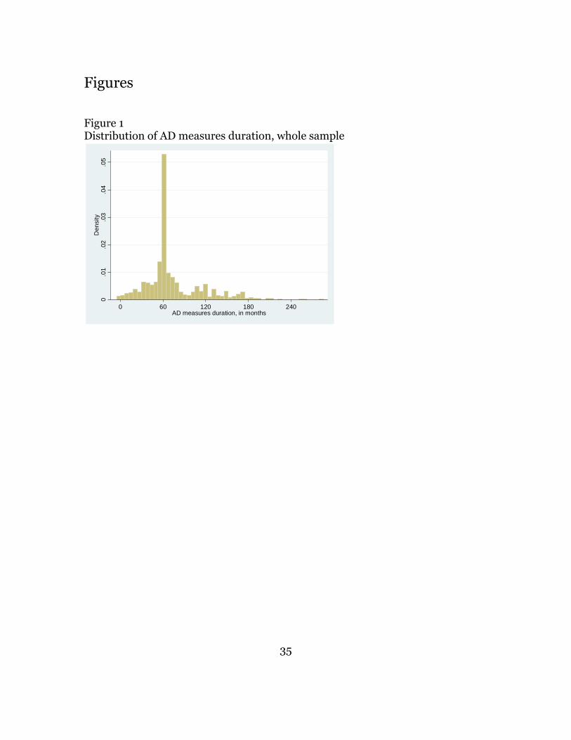
Figure 1 shows that although the five-year review is −unsurprisingly− the mode of

the distribution of durations, a substantial number of measures are terminated

before the 5-year review; moreover this is true even when censored observations

are taken out (they are included in Figure 1).

Figure 1 Distribution of AD measures duration, whole sample

Returning to the country data in Tables 1a-1b, the US stands out with a median

duration of 89 months (110 if censored observations are taken out). The US also

8

holds the record of maximum length at 285 months (23 years and nine

months).10 At the other extreme, Argentina is at a low 33 months.11 Other major

users (Australia, Canada, the EU, Mexico and South Africa) are at 60 months or

close to it, suggesting regular and effective five-year reviews. Overall, however,

the proportion of over-five-year measures is substantial: 44% on average, with

Canada (42%) and the EU (50%) on the low side and the US (68%) and Venezuela

(81%) on the high side.

Table 1a-1b Length of AD measures: descriptive statistics by determination country Figure 2 collects graphs of the duration of AD measures for a few countries. It

suggests that, over time, the duration of AD measures has been trending down,

although one has to be careful to filter out the effect of censoring towards the end

of the sample period. Thus Figure 2 shows AD duration over time, by country,

plotted against the measures’ initiation year for both full country samples (plain

lines) and samples purged of censored observations (dotted lines). Looking at the

latter, the curves are heading down since 1980 for the EU and since 1996 for the

US, with less clear-cut trends for other countries. Though Moore (2004) found,

as noted in the introduction, a positive coefficient on time in a probit of renewal

decisions, judging from the overall duration of measures, the unobserved

interaction between annual and expiry reviews seems to have worked to reduce

average measure duration in the US. Whether this is due to the WTO agreement

or not, however, must be assessed on the basis of parametric evidence (see next

10 This was case USA-AD-25 filed by Pq Corp. of Valley Forge, PA, in May 1980 against Rhône-Poulenc SA of France, which carried a duty of 60% and was revoked in October 2004. 11 Argentina sets duties at less than five years (typically three years). This is consistent with Article 11.3 of the AD Agreement, since this provision sets the maximum duration of measures. Chile not only sets the duration of duties at less than five years but also cuts off the life of measures at the end of the period chosen with no possibility of extension.

9

section). Interestingly, for Turkey, the WTO agreement seems to have stopped a

downward trend rather than encouraged it.12

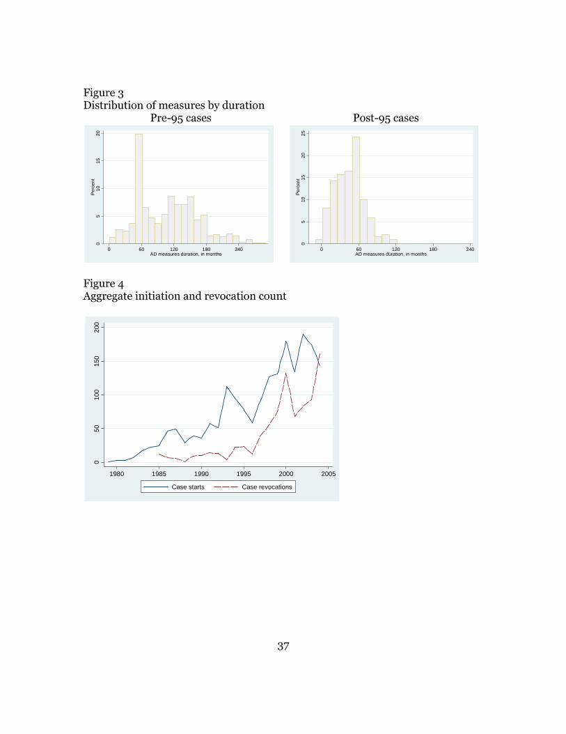
Figure 2 Duration of AD measures, selected determination countries Figure 3 shows the distribution of measures by their duration, before and after

the agreement. It can be seen that, in the second period, the mass of measures

clearly shifts from over five years to under five years, suggesting that something

did happen.

Figure 3 Distribution of measures by duration Figure 4, which aggregates initiations and revocations over all countries, suggests

a parallel movement of initiations and revocations, so the rise of revocations

toward the end of the sample period is likely to be due at least partly to the rise of

measures “ripe for revocation” as much as the WTO agreement.

Figure 4 Aggregate initiation and revocation count

In sum, the evidence so far suggests that something did happen in the later years

of the sample period, but assessing what that is −the WTO agreement or

autonomous forces− calls for a more formal analysis.

12 At least in principle, the agreement could have had the effect of reducing the frequency of revocations at less than five years. In Mexico, for instance, an AD order could be revoked after just one year of no-dumping finding (a rule similar to the US 3-years-no-dumping). The perspective of a mandatory review at five years could thus reduce the frequency of requests for administrative reviews and thus of the dumping-margin recalculations that could otherwise have led to early termination.

10

3. Initiations & revocations: A five-year cycle?

This section estimates the relationship between AD measure revocations and

their initiations lagged five years. There are two natural break points. If the WTO

agreement had a de jure effect, the break point should be 2000, the year in which

the first “eligible” measures came up for review. If it had a de facto effect, the

break point could be 1995, after which countries knew that the rules had changed

and progressively put in place WTO-consistent procedures.

3.1 Estimation

3.1.1. The equation

The dependent variable is the count of revocations for each year/determination

country pair (the year/country is the unit of observation, with an effective sample

size of about 200 observations). The regressors include, first, the count of

initiations lagged five years broken into two parts: one interacted with a dummy

variable equal to one when the revocation year is after 2000 (“5-year lagged

starts, post-2000”) and one interacted with one minus that dummy (“5-year

lagged starts, pre-2000”). This is the crucial explanatory factor: As explained in

the introduction, if the WTO agreement had a de jure effect, we would expect this

coefficient to be higher and more precisely estimated when interacted with the

post-2000 dummy.

A similar variable is constructed using 1995 as the break point in order to test

whether countries significantly altered their behavior as soon as the agreement

was signed but before it became binding (revoking a 5-year old measure in 1998,

for instance, would not be mandated by the agreement and would therefore

reflect a political decision to comply).

11

Panel estimation takes care of unobserved time-invariant heterogeneity between

countries, but there may also be time-variant sources of heterogeneity. In

particular, country i’s revocation count at t is likely to be related to the number of

measures in force, which varies over time. In order to control for this, we include

the stock of existing measures for country i at time t as an “exposure” variable.13

We also split it between before and after the agreement in order to minimize the

scope for misspecification.

All regressions include time effects, not reported (in order to save space) except

for 2000. As mentioned, for measures straddling the pre- and post-agreement

periods (think of a measure put in place, say, in 1993 and still in force by 1995)

the 5-year clock would start ticking in 1995. Thus, a large stock of measures

adopted before 1995 and never revoked would all come up for mandatory review

in 2000, in particular in the US which did not have sunset reviews prior to the

UR agreement. This generates a peak of revocations in 2000 that is visible in the

data. Thus, the dummy variable for the year 2000 is of special interest, and we

will report its coefficient.

Finally, the regression is performed in levels; this is appropriate because

variables on the equation’s LHS (revocations) and RHS (initiations), although

non-stationary, are co-integrated.14

13 In an accident-count study, the equivalent would be, say, the annual number of kilometers travelled by an individual driver. Stata has a specific “exposure” option but its function is merely to constrain the parameter of the exposure variable to equal unity, a constraint that is rejected by the data. So we include the stock of cases as a regressor with no constraint. 14 A Maddala-Wu unit-root test for unbalanced panels accepts the hypothesis of co-integration of revocations and initiations at the 5% level.

12

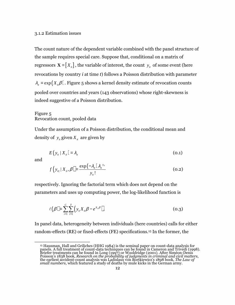
3.1.2 Estimation issues

The count nature of the dependent variable combined with the panel structure of

the sample requires special care. Suppose that, conditional on a matrix of

regressors [ ]itX=X , the variable of interest, the count ity of some event (here

revocations by country i at time t) follows a Poisson distribution with parameter

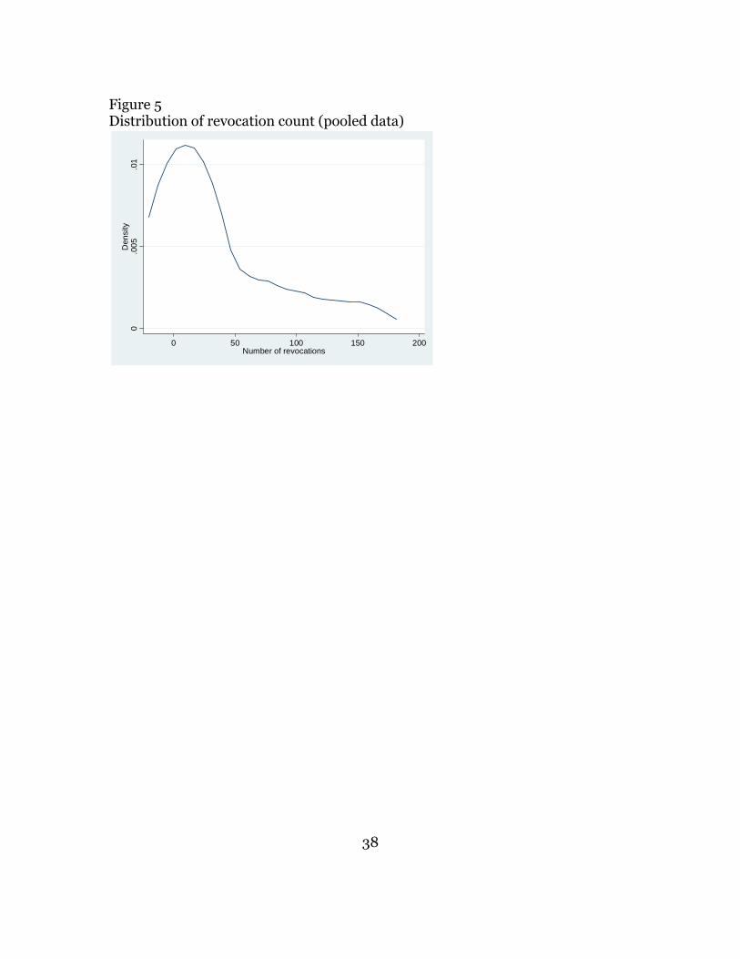
( )expit itXλ β= . Figure 5 shows a kernel density estimate of revocation counts

pooled over countries and years (143 observations) whose right-skewness is

indeed suggestive of a Poisson distribution.

Figure 5 Revocation count, pooled data Under the assumption of a Poisson distribution, the conditional mean and

density of ity given itX are given by

( )|it it itE y X λ= (0.1)

and

( ) ( )|

exp| ,

!

ityit it

it itit

f y Xy

λ λβ

−= (0.2)

respectively. Ignoring the factorial term which does not depend on the

parameters and uses up computing power, the log-likelihood function is

( ) ( )1 1

it

C TX

it iti t

y X e ββ β= =

= −∑∑� . (0.3)

In panel data, heterogeneity between individuals (here countries) calls for either

random-effects (RE) or fixed-effects (FE) specifications.15 In the former, the

15 Hausman, Hall and Griliches (HHG 1984) is the seminal paper on count-data analysis for panels. A full treatment of count-data techniques can be found in Cameron and Trivedi (1998). Briefer treatments can be found in Long (1997) or Wooldridge (2001). After Siméon-Denis Poisson’s 1838 book, Research on the probability of judgments in criminal and civil matters, the earliest accident-count analysis was Ladislaus von Bortkiewicz’s 1898 book, The Law of small numbers, which featured a study of deaths by mule kicks in the German army.

13

parameter of the Poisson distribution is assumed to be itself a random variable of

the form

it i itλ α λ=� (0.4)

where iα is a random country-specific effect with a gamma distribution. Thus, if

( )expit itXλ β= as before and ( )expi icα = for some random variable ic , then

( )expit i itc Xλ β= +� . In the fixed-effects (FE) specification, the individual effect ic is

taken as non-stochastic and the estimation is conditioned on the sum of the

counts for each individual, 1

T

itty

=∑ , which is itself a Poisson variable.

By assumption the Poisson distribution requires the mean and variance of the

count to be equal, which is not always (in fact, rarely) the case. Checking for

overdispersion requires first running a Poisson regression, retrieving the

estimated variance of the residuals and plotting it against the conditional mean of

the dependent variable, the unit of observation being here a country (a figure

similar to HHG’s Figure 1). Under the Poisson assumption, the ratio should be

around unity. A regression can also be run of the variance against the mean. We

found overdispersion,16 and accordingly used a negative binomial (NB) estimator.

The NB distribution makes the Poisson parameter itλ� itself a random variable

following a gamma distribution with parameters ( )expit itXλ β≡ and iθ .17 Then

( )it it iE y λ θ= and ( ) ( )var 1it i i ity θ θ λ= + . Under a RE specification, iθ is itself taken

as a random variable with ( )1/ 1 iθ+ following a beta distribution; under a FE

specification, iθ is non-random and the joint probability of the counts is, as

before, conditioned on their total by individual.

16 A regression of

2σ̂ on λ̂ gives 2 ˆˆ 3.91(3.68) 2.39(0.38)σ λ= − + (standard errors in parentheses)

so the hypothesis of zero intercept cannot be rejected but the unit slope is. The sample-wide averages of

2σ̂ and λ̂ are 20.12 and 8.92. 17 On this, see Allison and Waterman (2002). Note that here

itλ� follows a gamma distribution

whereas in the FE Poisson model it was ic that followed a gamma distribution.

14

3.1.3 Interpreting regression coefficients

Count-data regression coefficients can be reported either in standard form or in

so-called “incidence-rate ratio” (IRR) form. The “incidence rate” (here the

predicted revocation count) is ˆˆ exp( )it ity X β= and the effect of a unit increase in

regressor X on this incidence rate is

( ) IRR1

X

X

ee

e

ββ

β β− = ≡ . (0.5)

Thus, an IRR below one indicates a negative effect (i.e. is equivalent to a negative

coefficient in standard form), and conversely. Alternatively, if regressor X is

continuous, its marginal effect is

ˆ ˆ ˆ .it

j itijt

yy

xβ∂ =

∂ (0.6)

where ˆjβ is a standard-form coefficient. Thus, a marginal effect equal to one for

lagged initiations −one-for-one revocation of measures after five years− requires

ˆ1/ 0.13j ityβ = =� after substitution of the predicted revocation count.

3.1.4 Results

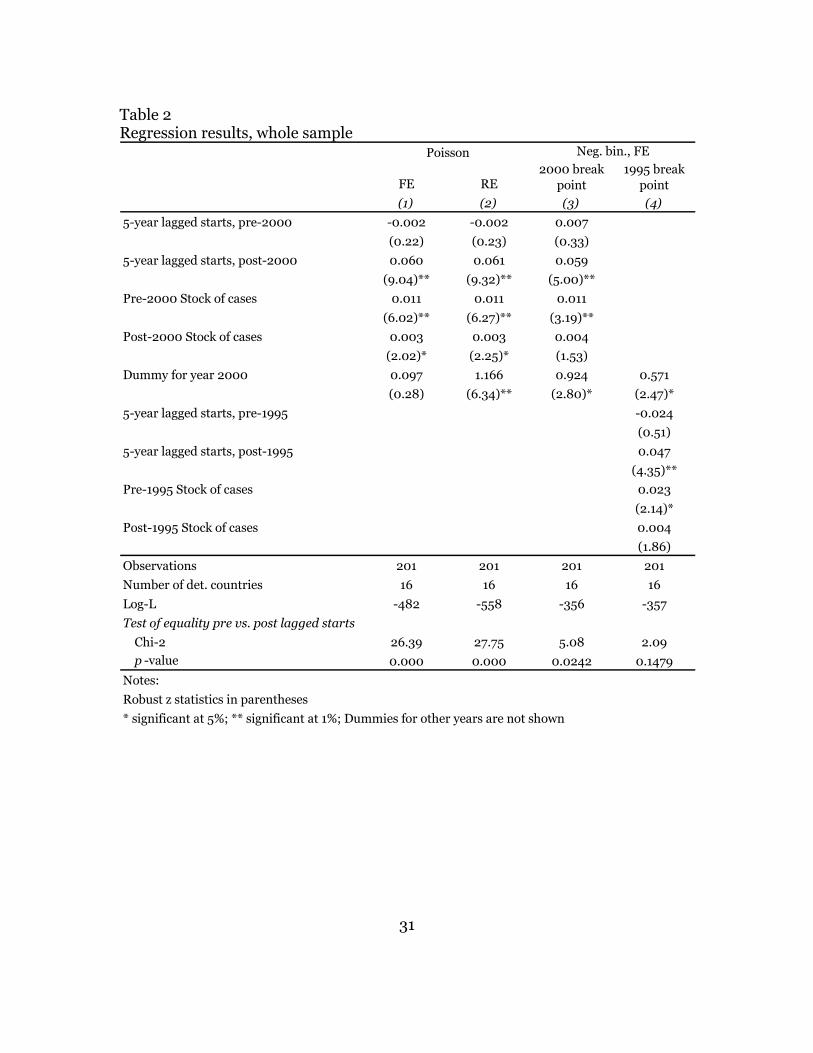
FE and RE Poisson estimates are reported in columns (1)-(2) of Table 2, all in

standard form. Note that they are very close; this being also the case for the NB

estimator, we report only FE estimates for the latter.

Table 2 Regression results, whole sample

15

Poisson coefficients on initiations lagged five years are insignificant before 2000

and positive and highly significant after; chi-squared tests of equality of

coefficients consequently reject the null hypothesis of equality at any level of

significance. This provides the first piece of evidence that the WTO agreement

had an effect. However even after 2000 the estimate is much lower than the 0.13

benchmark, with an implied marginal propensity to revoke measures at 5 years of

46% (against zero before, since the coefficient was insignificant). Consistent with

expectations, the ‘year 2000’ dummy variable was significant (and had the

highest coefficients of all time effects) under pooled and RE estimation but not

under FE where the “between-countries” dimension of the variability in

revocations is not used (the mopping up of old cases in 2000 essentially

concerned the US).

NB estimates using 2000 as the break point, reported in column (3), are close to

those of the Poisson estimator, which is to be expected, and thus again very far

from the levels that would give one-for-one revocations at five years. 18

A Chow (LR) test confirms the presence of a structural break in 2000 ( 2 3.82χ = ,

p-value 0.0508). Thus, using 2000 as the break point suggests that WTO

Members strengthened the five-year cycle once the agreement became binding,

evidence in favor of a de jure effect. Column (4) shows that using 1995 as a break

point, gives qualitatively similar estimates, but the null of equality is no longer

rejected by the Chi-square test, suggesting a weaker structural break.

Next, we explored the possibility that some WTO Members complied more

whole-heartedly than others by interacting the pre- and post-agreement count of

5-year-lagged initiations with country dummies and running separate tests for

the equality of coefficients before and after 2000. Results are reported in Table 3.

18 Using the negative binomial regression, the estimated marginal propensity to revoke measures at 5 years was 45% after the agreement (against 46% using Poisson).

16

Tests of equality of pre- and post-2000 cycle variables reject the null hypothesis

(no change) for Canada, Australia, Mexico and the EU. For the latter, however,

the change goes in the wrong direction (the cycle is less marked after than before

as the coefficient on initiations lagged five years goes down). Remarkably, for the

US, there is no trace of a five-year cycle either before or after 2000. Thus,

Moore’s conclusion that the US ‘shirked’ on the application of the WTO

agreement seems confirmed by the revocation data. The year 2000 is

nevertheless significant for the US, suggesting a WTO-consistent one-time

“mopping-up” of old measures.19

Table 3 Regression results by country 3.1.5 When did things really change?

Given the importance of the change’s timing, in the next exercise we turned the

question on its head and asked, assuming that there was a structural break (an

assumption consistent with the Chow test’s result), when would it be most likely

to have taken place? The problem can be expressed as a standard switching-

regression problem with unknown but exogenous cutoff. Let ity be the observed

number of revocations for country i and year t, 1ity and 2ity be two latent

variables and 1itu and 2itu two independent and Poisson-distributed error terms.

Suppose that the data-generating process is given by

( ) ( )( ) ( )

1 1 0 0 1

2 2 1 1 2

, exp ,

, exp ,

it i i i i

it i i i i

E y X c X c

E y X c X c

α β

α β

= + +

= + + (0.7)

1

2

if 1

otherwise,it t

itit

y Iy

y

==

(0.8)

19 As mentioned in Footnote 9 above, roughly a fifth of those measures were terminated because there was no domestic interest.

17

01 if

0 otherwiset

t tI

≥=

(0.9)

where ic is a country fixed effect, t is time since the beginning of the sample

period (1979 in our case) and 0t is the postulated breakpoint (the agreement plus

five years if the conjecture is true). The problem is to find the value of 0t , together

with the model’s other parameters, for which the likelihood of observing the

given data is highest. System (0.7)-(0.9) can be written in more compact form as

( ) ( )1 2 0 0 1 1 2, , exp 1it i i i t i t t i t iE y X X c I X I X cα β β= + + − + (0.10)

Except for the exponential form and distributional assumption, this is a standard

problem for which several methods are available (see Dutoit 2006 for a survey).

In a case where OLS was appropriate, Hansen (2000) proposed a grid-search

method based on the minimization (by choice of the cutoff point 0t ) of the sum of

squared errors. An obvious alternative here is the maximization of the maximum

likelihood (the “maximum-maximorum”, henceforth MM).

We performed a grid search over sample- split years between 1990 and 2005

using the fixed-effects Poisson estimator and then plotted the maximum

likelihood as a function of time. The result is shown in the left-hand side panel

(iii) in Figure 6. It can be seen that it peaks somewhere between 1995 and 2000,

although 2000 is not any better than pre-Uruguay Round years. Given that the

Chow test already gave indication of a structural break, this last observation

should probably not be taken too seriously recalling that the sample period’s early

years contain the bulk of the sample’s missing values and are thus not very

informative.

Figure 6 Log likelihood as a function of the break year, true and simulated data

18

Nevertheless, as a check we generated a simulated data set mimicking as closely

as possible our sample but embodying a time break at t = 20 (corresponding to

year 2000 in our sample). A scatter plot of the dependent variable against time

and a kernel density estimate are shown in the right-hand side panels of Figure 6

for comparison with the true ones (on the left-hand side). It can be seen that the

simulated sample mimics fairly well the true one. The data-generating equations

are given in Appendix 1. Then we performed a series of grid searches (one for

each simulated sample, with a new random error drawn each time) identical to

the one we performed on the true sample and plotted the resulting MM curves.

One such curve is shown in the last panel of Figure 6. The peak at the true sample

split is very clear, suggesting that if 2000 was a strong trend break we should

probably have sharper results in terms of the MM curve’s shape. Thus, it is fair to

say that the “structural break at 2000” signal, while there, is a relatively faint one.

4. Shorter AD measures?

4.1 Non-Parametric Survival Analysis

We now turn to a survival analysis of individual AD measures. This is instructive

on three counts. First, from a substantive point of view, what we are interested in

is not just the WTO’s ability to impose a five-year cycle, but also, and perhaps

more importantly, its ability to reduce the duration of trade-distorting AD

measures. Second, making AD measures the unit of observation dispenses with

the need for aggregation. Third, the bilateral nature of the AD database provides

us with a quasi-experiment setting. The reason is that some measures (about a

third of them) were taken against countries that were not members of the WTO.

Those measures were covered by the agreement neither before nor after 1995;

they accordingly provide a “control group” against which to benchmark the

19

change observed in the duration of measures taken against WTO members (the

“treatment group”) after the agreement.

As WTO membership is voluntary, it might be argued that our setting is not one

of “natural experiment” but rather one of “treatment effect”, where individuals

may choose the treatment because they have unobserved characteristics that raise

its return (like ability for schooling decisions). If such were the case, better

outcomes (shorter measures) attributed to the treatment would actually be a

reflection of unobserved characteristics (say stronger bargaining power) rather

than of the agreement itself. However this potential endogeneity bias is unlikely

to apply here. Most of our WTO members are GATT-1947 founding signatories

and the main non-members, China and Russia, are so because they are formerly

Communist countries. Thus, it is hard to think of any conceivable selection bias

and the treatment can pretty well be considered as “forced”.

Let t be “analysis time”, i.e. time since the onset of risk, which for each AD

measure is the year in which final duties were put in place (what we have called

the initiation year, the ‘risk’ being that of revocation), T be the date of revocation

measured again in “analysis time”, and let ( ) ( )probF t T t= ≤ be the cumulative

distribution function of the time of revocation, with density f . The corresponding

survival and hazard functions are defined as ( ) ( )1S t F t= − and ( ) ( )0

tH t h dτ τ= ∫

respectively, where ( ) ( ) ( )1h t f t F t= − is the distribution’s hazard rate. It can

be shown that ( )H t and ( )S t are related by ( ) ( )lnH t S t= − . Finally let tn and

ty be respectively the stock of AD measures in force (“individuals at risk”) and the

number of revocations (“deaths”) at t months. The Kaplan-Meier (KM) estimator

of ( )S t is calculated as

20

( )1

ˆ 1t y

S tn

τ

τ τ=

= −

∏ ; (0.11)

that is, the KM estimator of ( )S t is the product of per-period survival-probability

estimates calculated as one minus death frequencies, from the onset of risk up to

time t.

As discussed, we take the target country’s WTO membership status as the

criterion for treatment vs. control groups: the treatment group is that of AD

measures against WTO members (subject to WTO disciplines) whereas the

control group is that of AD measures against non-members (not subject to WTO

disciplines). As for the pre- vs. post-treatment dimension, things are more

complicated. The “treatment” applies to AD measures initiated after 1995. Quid

of a measure that started, say, in 1989, survived past 1995, and was revoked later

on? As explained in section 2.3, for a pre-agreement measure having survived

past 1995, the sunset-review clock would start ticking in 1995, implying a

mandatory review in 2000. Based on this, we split our sample as follows. The

“pre-agreement” period covers measures initiated before 1995 and revoked prior

to or in 1995. Measures still in force by 1995 are treated as censored. The “post-

agreement” period covers measures initiated in 1995 or later; measures still in

force by the sample period’s end (2005) are treated as censored. Pre-1995

measures that were in force in 1995 are considered as new measures in the post-

agreement period, as if they had changed identity.20

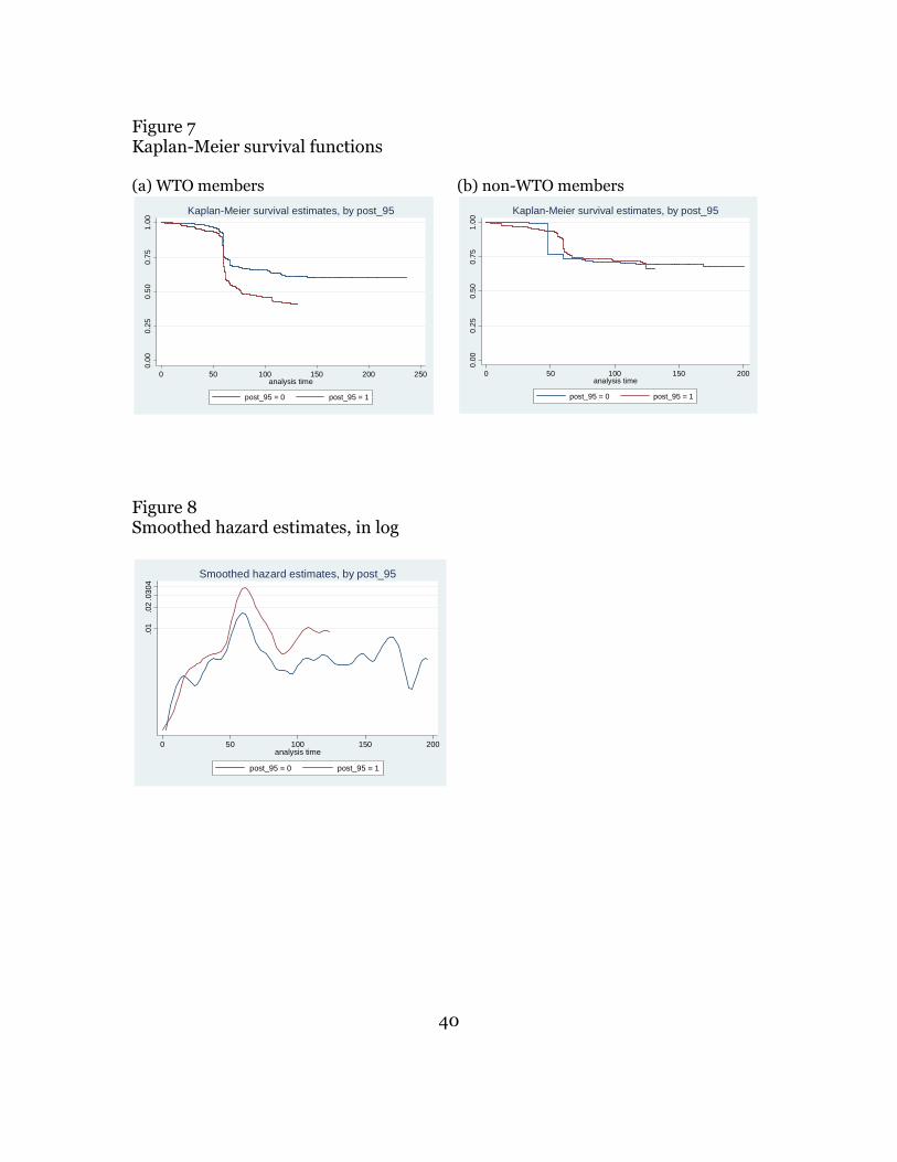
Graphs of KM estimates are shown for WTO members and non-members in the

two panels Figure 7 respectively. For WTO members (panel a), the post-

agreement survival curve is below the pre-agreement one, meaning that measures

20 This implies double counting of measures straddling the pre- and post-agreement periods. Treating these measures as pre-agreement ones (and therefore counting them only once) alters none of our results.

21

die faster, and a larger part of the difference is in the size of the jump down at 60

months (5 years).

Figure 7 Kaplan-Meier survival functions

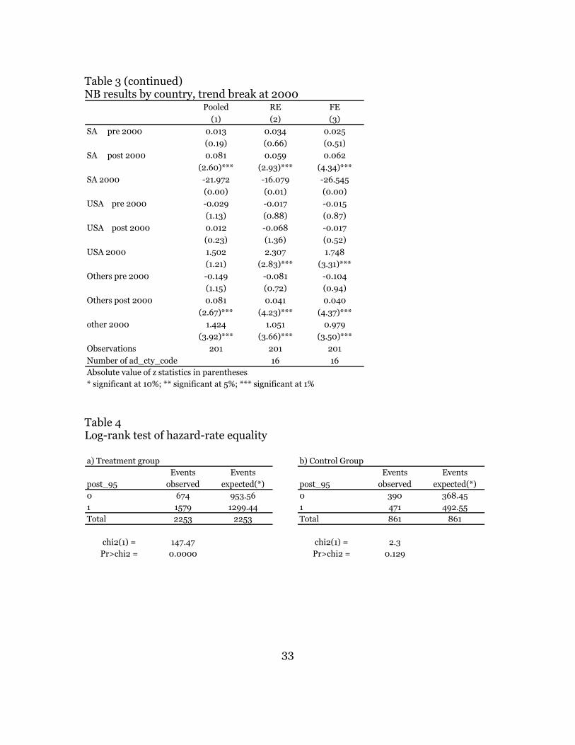
A log-rank test of the null hypothesis ( ) ( )0 0 1:H h t h t= (equality of hazard rates, a

Chi-squared (1) when there are two alternatives), reported in Table 4 (a), rejects

the null at any conceivable level of significance.21

Table 4 (a-b) Log-rank test for equality of survivor functions Thus, the outcome changed without ambiguity for the treatment group. For the

control group, Panel (b) of Figure 7 and of Table 4 (b) shows that the “treatment”

had no effect.

In order to verify that this effect is not driven by heterogeneity between the

treatment and control groups (“overt bias”), we now turn to a semi-parametric

approach.

4.2 Semiparametric Cox Regression

We now run a difference-in-differences Cox regression controlling for each

measure’s sector, determination country, investigated country and for time. Cox’s

proportional-hazard model (Cox 1972) is a semi-parametric one whose basic

assumption is that the conditional hazard function is separable between time and

covariates; that is,

( ) ( ) ( )0, ,h t h tβ φ β=x x (0.12)

21 We also performed Wilcoxon tests and got the same answer.

22

where the first factor on the RHS is the “baseline hazard” and is a function of t

alone, while the second is a function of the covariates alone. Cox’s model does not

assume any particular form for the baseline hazard, which entails a loss of

efficiency compared to fully parametric Weibull or Gompertz models but reduces

the risk of mis-specification.22

Is the proportional-hazards (PH) assumption appropriate? Figure 8 shows

smoothed hazard-function estimates for the treatment and control groups in logs.

Under the PH assumption, the log curves should be roughly parallel to each

other.

Figure 8 Smoothed hazard estimates, in logs A Schoenfeld test of the proportional-hazards assumption accepts the null of

proportional hazards across groups (WTO membership, first line of Table 5)

across periods (pre- and post-treatment, second line) and across their interaction

(third line).

Table 5 Test of proportional hazards assumption

The form of the function ( ).φ reflects both the usual exponential form and the

difference-in-differences approach:

( ) {

}1 2 3

4 5 6 7

exp WTO POST POST WTOi i i i i

D Ii i i i i

D D D D

HS C C t u

φ β β β β

β β β β

= + +

+ + + + +

x (0.13)

In (0.13), i indexes AD measures (the unit of observation), POSTiD and WTO

iD are

dummy variables marking respectively the post-treatment period and WTO

22 In Cox’s model, the baseline hazard cancels out from the likelihood function because of the assumption of proportional hazards, which is why it is called a partial or pseudo-likelihood function.

23

membership of the target country, and 3β̂ measures the treatment’s effect. iHS ,

i

DC , i

IC and it are controls for the AD measure’s industry (by HS section),

determination country (the one imposing the measures), investigated country

and year of determination.

Table 6 (a-b) Cox regression results (robust) Table 6 shows the regression results. All coefficients are in “exponentiated” form

and can be interpreted pretty much like incidence-rate ratios in count models:

they give the ratio of the hazard rates for a change in the corresponding dummy

from zero to one, so a value above one indicates a positive effect and a value

between zero and one a negative effect. For instance, the effect of WTO

membership of the investigated country on the hazard rate of AD measures

before the agreement is

( )( )

( ) ( )( ) ( ) ( )( )

0 1

10

ˆˆ exp1, 0, ˆexpˆ exp 00, 0,

exp 0.211

1.235.

WTO POST

WTO POST

h th t D D

h th t D D

βββ

β= =

= == =

==

(0.14)

Because this estimate is above one, the effect of WTO membership on the hazard

rate of measures is positive: they die 23.5% faster than when the investigated

country is not a member, a result in conformity with the KM curves. What we are

particularly interested in is whether the agreement had any effect once outside

influences on the duration of measures are controlled for. Controls for:

determination country, investigated country, industry and initiation year are

introduced one by one from column (1) to column (5). It can be seen that the

coefficient on WTO*Post agreement, which gives a consistent estimate of the

treatment’s effect, is robustly above one and always significant at the 1% level.

24

The introduction of controls actually raises its value, except for the time controls

−column (5)− which seem to confound the effect of the agreement.

As a further check, we ran the same regression but stratifying the estimation by

the covariates’ categories, a technique that is more robust to violations of the

proportional-hazards assumptions. The results, reported in Table 6b, are

essentially same.

Thus, conditional on the covariates, the WTO agreement significantly raised the

hazard rate of AD measures against WTO members and even more so when the

counterfactual is what happened to measures against non-members −strong

evidence in favor of “forced” or de jure compliance.

5. Concluding remarks

Summing up, the count-data evidence is suggestive of a stronger five-year cycle

for AD measures covered by the WTO agreement than for others, whereas the

survival-rate evidence is suggestive of a somewhat shorter duration due to a jump

down in the survival function at five years. Can that be taken to mean that the

WTO was successful in its effort to bring AD measures under an effective

discipline of five-year sunset reviews?

A WTO agreement, like any agreement between sovereign nations, is bound to

reflect a mixture of free political will and coercion through package-dealing.

Thus, there can be two components to the agreement’s effect: a de jure or binding

component and a de facto or political component. We tried to disentangle these

two components using several identification strategies. First, we used the count

analysis to identify where the structural break was: in 2000, when the first

mandatory reviews appeared, or in 1995, when the agreement was signed but not

25

yet binding? The answer we found in the data can be summarized as “in 2000,

but 1995 is also OK”. Second, also using the count data we looked at compliance

by country and found that the US, which was the only major AD user that was

forced by the agreement to adopt the practice of sunset reviews (other large users

already had sunset-review provisions) nevertheless did not alter its practices,

making the reviews largely perfunctory. Third and last, using the database’s

bilateral structure, we split the survival analysis according to whether target

countries were WTO members or not. We found that, after controlling for

relevant covariates, the “treatment group” (AD measures against WTO members,

for which WTO disciplines would apply after 1995) seemed to have been affected

by the post-1995 treatment significantly more than the “control group” (AD

measures against non-members, for which WTO disciplines would not bind even

after 95). All in all, the data’s verdict through a variety of approaches is in favor of

a substantial de jure component in the agreement’s effect. Put differently, the

agreement does not seem to have merely validated a change in the mood of

member countries.

This conclusion must be nuanced by the fact that the US did not introduce a clear

five-year cycle in its AD measures, although this might arguably have been the

agreement’s primary goal. This last observation raises a question. If the US

disliked Article 11.3 of the ADA as much as it seems to, why did it sign it in the

first place? There may be several answers. First, the Uruguay Round Agreement

was a package and not every Member liked everything in it. Second, Article 11.3’s

wording was so loose that it made almost-systematic continuation of measures an

easy option −albeit not consistent with the agreement’s spirit− since it was

unlikely to be taken to the DSB. Lastly, there may have been something of a

“double dupes’ deal” at the WTO in that the US did not quite get the “deferential

attitude” it was hoping for from panels, and especially from the Appellate Body,

on the basis of Article 17.6; while Members wishing for strengthened AD

26

disciplines failed to convince the US to go with the spirit of the sunset-review

agreement.

Opposition to any relaxation in the force of AD regulations still runs strong. For

instance, sixty-two Senators including the majority and minority leaders recently

signed a letter to President Bush expressing their continued opposition to any

agreement that would weaken trade remedy laws. However, positions may

gradually evolve as AD use by emerging countries intensifies and the US

increasingly finds itself, as was already noted in a 1998 report of the

Congressional Budget Office (CBO 1998), on the receiving side (it currently ranks

second only to China as an AD target).

27

References

Allison, Paul D. and Richard Waterman (2002), “Fixed effects negative binomial regression models”, in Ross Stolzenberg, ed., Sociological Methodology 2002, Blackwell. Australian Customs Service (2000), Australia’s Antidumping and Countervailing Administration; Australian Government. Blonigen, Bruce and Jee-Hyeong Park (2004), “Dynamic Pricing in the Presence of Antidumping Policy: Theory and Evidence”; American Economic Review 94, 134-154. Bown, Chad (2006), “Global Antidumping Database version 2.1”; mimeo, Brandeis. Cameron, A. Colin and P. K. Trivedi (1998) Regression Analysis of Count Data, Cambridge University Press. − (2005), Microeconometrics: Methods and Applications, Cambridge University Press. Cleves, Mario; W. W. Gould and R.G. Gutierrez (2004), An Introduction to Survival Analysis Using Stata; revised ed., Stata Corp.

Congressional Budget Office (1998), Antidumping Action in the United States and Around the World: An Analysis of International Data; CBO paper. Cox, David R. (1972), “Regression Models and Life Tables Iwith Discussion)”; Journal of the Royal Statistical Society B 24, 406-424. Dutoit, Laure (2006), “Switching-regression and Selection Models: A Survey”, mimeo, University of Lausanne. Hansen, Bruce (2000), “Sample Splitting and Threshold Estimation”; Econometrica 68, 575-603. Hausman, Jerry A.; Bronwyn H. Hall and Zvi Griliches (1984), "Econometric Models for Count Data with an Application to the Patents-R&D Relationship"; NBER Technical Working Papers 0017, National Bureau of Economic Research, Inc.

28

Horlick, Gary (1993), “How the GATT Became Protectionist: An Analysis of the Uruguay Round Draft Final Antidumping Code”; Journal of World Trade 27, 5-17. Howse, Robert, and R. Staiger (2005), “United States-Sunset Revies of Anti-Dumping Duties on corrosion-Resistant Carbon Steel Flat Products From Japan, AB-2003-5, A Legal and Economic Analysis of the Appellate Body Ruling”. Ikenson, Daniel (2005), “Shell Games and Fortune Tellers: The Sun Doesn’t Set at the Antidumping Circus”; Free Trade Bulletin 18, Center for Trade Policy Studies, Cato Institute. Im, K. S., Pesaran, M. H., and Shin. Y. (2003), “Testing for Unit Roots in Heterogenous Panels, Journal of Econometrics 115 (revise version of 1997’s work), 53-74. Levin A., Lin C.F., and Chu C.J. (2002), “Unit Root tests in Panel Data: Asymptotic and finite-sample properties”, Journal of Econometrics 108 (revise version of 1992’s work), 1-24. Liebman, Benjamin (2001), “ITC Voting Behaviour on Sunset Reviews”; mimeo. Long, Scott (1997), Regression Models for Categorical and Limited Dependent Variables; Sage. Maddala, G. S., and S.Wu(1999), “A Comparative study of unit root tests with panel data and a new simple test”, Oxford Bulletin of Economics and Statistics, Special issue, 631-652. Moore, Michael (1999) “Antidumping Reform in the US: A Faded Sunset” Journal of World Trade 33, 1-88. − (2002) “Commerce Department Antidumping Sunset Reviews: First Assessment,” Journal of World Trade 36, 675-698. − (2004), “Can the US Dump Antidumping? Evidence from Past ‘Reforms’”; mimeo. − (2006), “An Econometric Analysis of US Antidumping Sunset Review Decisions” Weltwirtschaftliches Archiv 142. Vermulst, Edwin, and p. Waer (1996), E.C. Antidumping Law and Practice; Sweet & Maxwell.

29

Tables Table 1a Length of AD measures: descriptive statistics by determination country c/

Obs Mean Median

Std.

Dev. Min Max

Censored

# of obs. a/

% of

censored

obs.

# of obs.

over 5 years

b/

% of

over-5-

years

(1) (2) (3) (4) (5) (6) (7) (8) (9) (10)

Argentina 117 33 33 15 0 73 51 44% 4 3%

Australia 64 50 49 24 18 121 32 50% 13 20%

Canada 201 75 60 40 6 236 58 29% 84 42%

China 75 27 27 18 3 79 63 84% 6 8%

Colombia 19 66 60 38 0 130 1 5% 5 26%

European Union 252 68 60 34 9 183 90 36% 127 50%

India 276 46 43 20 7 129 156 57% 68 25%

Indonesia 17 22 14 26 0 67 11 65% 4 24%

Mexico 114 71 61 43 2 183 52 46% 68 60%

New Zealand 14 48 45 37 12 113 13 93% 5 36%

Peru 12 17 14 12 2 40 12 100% 0 0%

South Africa 128 69 64 28 14 155 62 48% 85 66%

South Korea 48 50 41 30 1 140 19 40% 15 31%

Taiwan 16 51 61 21 11 74 3 19% 9 56%

Turkey 121 44 35 30 4 111 92 76% 33 27%

USA 479 106 89 64 1 285 261 54% 325 68%

Venezuela 16 67 69 21 4 100 11 69% 13 81%

Total 1'969 68 60 48 0 285 987 50% 864 44%

Notes

a/ Cases whose revocation date is coded is coded as "IF" (in force)

b/ Cases whose length is over 60 months

c/ Cases with incompatible dates (init.date posterior to revocation date) taken out of the sample

30

Table 1b Descriptive statistics for uncensored observations only

Obs Mean Median Std. Dev. Min Max

Argentina 66 29 31 13 0 62

Australia 32 60 60 25 18 121

Canada 143 77 60 32 32 183

China 12 22 12 21 3 53

Colombia 18 69 60 37 0 130

European Union 162 65 60 27 17 177

India 120 48 55 15 15 71

Indonesia 6 44 67 34 0 67

Mexico 62 67 61 31 2 146

New Zealand 1 63 63 63 63

Peru 0

South Africa 66 64 63 21 16 113

South Korea 29 56 54 29 1 140

Taiwan 13 51 61 23 11 74

Turkey 29 86 93 22 49 111

USA 218 108 110 56 1 285

Venezuela 5 46 49 25 4 65

Total 982 71 60 42 0 285

31

Table 2 Regression results, whole sample

FE RE2000 break

point

1995 break

point

(1) (2) (3) (4)

5-year lagged starts, pre-2000 -0.002 -0.002 0.007

(0.22) (0.23) (0.33)

5-year lagged starts, post-2000 0.060 0.061 0.059

(9.04)** (9.32)** (5.00)**

Pre-2000 Stock of cases 0.011 0.011 0.011

(6.02)** (6.27)** (3.19)**

Post-2000 Stock of cases 0.003 0.003 0.004

(2.02)* (2.25)* (1.53)

Dummy for year 2000 0.097 1.166 0.924 0.571

(0.28) (6.34)** (2.80)* (2.47)*

5-year lagged starts, pre-1995 -0.024

(0.51)

5-year lagged starts, post-1995 0.047

(4.35)**

Pre-1995 Stock of cases 0.023

(2.14)*

Post-1995 Stock of cases 0.004

(1.86)

Observations 201 201 201 201

Number of det. countries 16 16 16 16

Log-L -482 -558 -356 -357

Test of equality pre vs. post lagged starts

Chi-2 26.39 27.75 5.08 2.09

p -value 0.000 0.000 0.0242 0.1479

Notes:

Robust z statistics in parentheses

* significant at 5%; ** significant at 1%; Dummies for other years are not shown

Poisson Neg. bin., FE

32

Table 3 NB results by country, trend break at 2000

Pooled RE FE

(1) (2) (3)

Australia pre 2000 0.122 0.112 0.102

(1.63) (2.39)** (2.44)**

Australia post 2000 0.194 0.179 0.165

(1.69)* (1.78)* (1.97)**

Australia 2000 -0.352 -0.091 -0.138

(0.26) (0.09) (0.14)

Canada pre 2000 0.083 0.109 0.091

(2.83)*** (4.51)*** (4.24)***

Canada post 2000 0.149 0.147 0.142

(2.85)*** (4.10)*** (5.22)***

Canada 2000 0.415 0.381 0.363

(0.40) (0.85) (0.80)

EU pre 2000 0.069 0.085 0.071

(1.57) (1.97)** (2.21)**

EU post 2000 0.064 0.042 0.048

(2.26)** (3.06)*** (4.49)***

EU 2000 -0.835 -0.809 -0.750

(0.77) (1.16) (1.10)

Mexico pre 2000 0.045 0.084 0.061

(0.88) (1.85)* (1.57)

Mexico post 2000 0.207 0.153 0.144

(2.18)** (1.97)** (2.33)**

Mexico 2000 -2.057 -1.288 -1.198

(1.17) (1.14) (1.15)

NZ post 2000 -17.735 -11.552 -23.062

(0.00) (0.02) (0.00)

NZ 2000 -20.920 -14.688 -26.253

(0.00) (0.00) (0.00)

33

Table 3 (continued) NB results by country, trend break at 2000

Pooled RE FE

(1) (2) (3)

SA pre 2000 0.013 0.034 0.025

(0.19) (0.66) (0.51)

SA post 2000 0.081 0.059 0.062

(2.60)*** (2.93)*** (4.34)***

SA 2000 -21.972 -16.079 -26.545

(0.00) (0.01) (0.00)

USA pre 2000 -0.029 -0.017 -0.015

(1.13) (0.88) (0.87)

USA post 2000 0.012 -0.068 -0.017

(0.23) (1.36) (0.52)

USA 2000 1.502 2.307 1.748

(1.21) (2.83)*** (3.31)***

Others pre 2000 -0.149 -0.081 -0.104

(1.15) (0.72) (0.94)

Others post 2000 0.081 0.041 0.040

(2.67)*** (4.23)*** (4.37)***

other 2000 1.424 1.051 0.979

(3.92)*** (3.66)*** (3.50)***

Observations 201 201 201

Number of ad_cty_code 16 16

Absolute value of z statistics in parentheses

* significant at 10%; ** significant at 5%; *** significant at 1% Table 4 Log-rank test of hazard-rate equality a) Treatment group b) Control Group

Events Events Events Events

post_95 observed expected(*) post_95 observed expected(*)

0 674 953.56 0 390 368.45

1 1579 1299.44 1 471 492.55

Total 2253 2253 Total 861 861

chi2(1) = 147.47 chi2(1) = 2.3

Pr>chi2 = 0.0000 Pr>chi2 = 0.129

34

Table 5 Test of Proportional hazards assumption

rho chi2 df Prob>chi2

WTO member 0.00122 0.01 1 0.9112

Post agreement 0.00999 0.03 1 0.8741

WTO*Post agreement -0.0187 0.73 1 0.3921 Table 6 (a) Cox regression results (robust)

(1) (2) (3) (4) (5)WTO member 1.235*** 1.259 0.617 0.435* 0.114***

(3.19) (0.61) (1.14) (1.81) (4.61)

Post agreement 0.953 0.745*** 0.845** 0.686*** 0.130***

(0.66) (3.92) (2.26) (4.66) (10.76)

WTO*Post agreement 1.743*** 2.355*** 2.535*** 2.713*** 1.860***

(6.57) (9.73) (10.40) (10.38) (5.59)

Controls

Investigated country no yes yes yes yes

Section no no yes yes yes

Determination country no no no yes yes

Initiation year no no no no yes

Observations 9484 9484 9484 9484 9484 significant at 10%; ** significant at 5%; *** significant at 1% Determination & investigated country, section and time effects not shown.

(b) Stratified Cox regression results (robust)

(1) (2) (3) (4) (5)

WTO member 1.235*** 1.238 1.218 0.118*** 0.014***

(3.19) (0.52) (0.38) (2.97) (4.83)

Post agreement 0.953 0.778*** 1.829*** 1.892*** 1.643

(0.66) (3.61) (6.23) (4.30) (0.93)

WTO*Post agreement 1.743*** 2.448*** 1.384*** 1.903*** 1.734***

(6.57) (10.55) (2.89) (3.98) (3.10)

stratified by

Investigated country no yes yes yes yes

Section no no yes yes yes

Determination country no no no yes yes

Dummies for Initiation years no no no no yes

Observations 9484 9484 9484 9484 9484 * significant at 10%; ** significant at 5%; *** significant at 1% (1): Determination & investigated country, section and time effects not shown. (2): Stratification by investigated country. (3): Stratification by investigated country and by HS section. (4): Stratification by determination and investigated country and by HS section. (5): With time effects. Time effects not shown. All coefficients in exponentiated form.

35

Figures Figure 1 Distribution of AD measures duration, whole sample

0.0

1.0

2.0

3.0

4.0

5D

ensi

ty

0 60 120 180 240AD measures duration, in months

36

Figure 2 Duration of AD measures, by determination country and initiation year

Argentina Turkey

020

4060

80A

v. c

ase

Dur

atio

n

1994 1996 1998 2000 2002 2004Case starting year

All cases Uncensored only

05

01

00A

v. c

ase

Dur

atio

n

1990 1995 2000 2005Case starting year

All cases Uncensored only

China India

020

4060

80A

v. c

ase

Dur

atio

n

1996 1998 2000 2002 2004Case starting year

All cases Uncensored only

020

4060

8010

0A

v. c

ase

Dur

atio

n

1990 1995 2000 2005Case starting year

All cases Uncensored only

EU US

05

01

0015

020

0A

v. c

ase

Dur

atio

n

1980 1985 1990 1995 2000 2005Case starting year

All cases Uncensored only

050

100

150

200

Av.

cas

e D

urat

ion

1980 1985 1990 1995 2000 2005Case starting year

All cases Uncensored only

37

Figure 3 Distribution of measures by duration

Pre-95 cases Post-95 cases

05

1015

20

Per

cent

0 60 120 180 240AD measures duration, in months

05

1015

202

5P

erce

nt

0 60 120 180 240AD measures duration, in months

Figure 4 Aggregate initiation and revocation count

050

100

150

200

1980 1985 1990 1995 2000 2005

Case starts Case revocations

38

Figure 5 Distribution of revocation count (pooled data)

0.0

05.0

1D

ensi

ty

0 50 100 150 200Number of revocations

39

Figure 6 Log likelihood as a function of the break year, true and simulated data

True sample Simulated sample a/ (i) Scatterplot

020

406

0(m

ean

) nr

0 10 20 30time

050

100

150

y

0 5 10 15 20 25time

(ii) Kernel density estimate of count

0.0

05.0

1D

ensi

ty

0 50 100 150 200Number of revocations

0.0

05.0

1.0

15

Den

sity

0 50 100 150ag_y

(iii) Maximum-maximorum of log-likelihood

-620

-600

-580

-560

log

_L

1990 1995 2000 2005break_est

-131

0-1

300

-129

0-1

280

-127

0lo

g_L

5 10 15 20 25break_est

Notes: a/ True break in time trend at t = 20

40

Figure 7 Kaplan-Meier survival functions (a) WTO members (b) non-WTO members

0.00

0.25

0.5

00.

751.

00

0 50 100 150 200 250analysis time

post_95 = 0 post_95 = 1

Kaplan-Meier survival estimates, by post_95

0.0

00.

250.

500.

751.

00

0 50 100 150 200analysis time

post_95 = 0 post_95 = 1

Kaplan-Meier survival estimates, by post_95

Figure 8 Smoothed hazard estimates, in log

.01

.02

.03.0

4

0 50 100 150 200analysis time

post_95 = 0 post_95 = 1

Smoothed hazard estimates, by post_95

41

Appendix 1: Data-generating model for simulations The following equations were used to generate a sample with two features: (i) it had a trend break at t = 20 (corresponding to the year 2000 in our true sample), (ii) it mimicked as closely as possible the true sample up to a scaling factor (of 4). In the model, x stands for the “exposure” variable (stock of cases or number of cases 4-6 years old).

( ) ( )1/ 43/ 2 4 if 8

0 otherwise;it

t tx

− >=

(0.15)

gamma(1);u ∼ (0.16)

( )

( )

int exp 0.01 0.5 20 if 202

int exp 0.01 otherwise.2

it

it

it

ui x t t

yu

i x

+ + − ≥ =

+

(0.17)

Up to the scaling factor, the resulting dependent variable has the same mean (about 5) but a higher dispersion than the true one (14.8 against 8.11). The choice of a gamma distribution instead of a Poisson one was for convenience only, as Stata has a built-in command generating a random variable with a gamma distribution but not a Poisson one.