Chapter 9

Propagation

The discussion so far has neglected mention of how radar signals propagate to and from the target. In a homogeneousmedium, radio wave propagation is by direct line of sight. The Earth’s atmosphere and ionosphere constitute aninhomogeneous medium, however, and spatial variations in the index of refraction (as well as ground effects) mustbe considered. The curvature of the Earth limits the distance over which line-of-sight communication occurs, but thiscan be extended by diffraction, refraction, reflection, andscattering in the atmosphere and ionosphere, and by groundeffects. The extension may be advantageous, as in the case ofdistant-object tracking, or may simply present additionalrange clutter, as in the case of aircraft or weather system tracking.

In the lower atmosphere, variations in the index of refraction n at commonly-used radar frequencies arise fromvariations in the neutral temperature, pressure, water vapor content, and liquid water content according to the formula

N ≡ (n− 1) × 106 = 77.6P

T+ 3.73 × 105Pw

T 2+ 1.4W (9.1)

whereN is called the refractivity,P is atmospheric pressure in mbar,T is temperature in Kelvin,Pw is the partialpressure of water vapor, andW is liquid water content in grams per cubic meter. The first term on the right sideof (9.1) is associated with the polarizability of air molecules, the second with permanent dipole moments of watervapor molecules, and the last with scattering from water droplets of some representative size. Except during extrememeteorological conditions, deviations in the index of refraction are generally limited to a few hundred parts per mil-lion. Nevertheless, it is possible for waves in the VHF and UHF bands to undergo sufficient refraction in the loweratmosphere and to propagate over paths significantly longerthan line-of-sight propagation would allow. From a radarperspective, this can permit the detection of targets at much greater ranges than might otherwise be possible. This canlead to confusion, particularly if the echoes are range aliased.

In contrast, variations in the index of refraction that occur in the upper atmosphere and ionosphere can be sub-stantial (up to 100%) at HF frequencies. This is what permitsshortwave radio signals to propagate around the Earth.So-called “over the horizon” (OTH) radars operate at HF frequencies and utilize long propagation paths to track aircraftand ships at distances of thousands of kilometers. The propagation paths taken by OTH radar signals are complicatedand highly variable. Predicting them requires large numerical models driven by routine and extensive ionosphericmeasurements from the ground and from space. The problem of inverting OTH radar signals is an active area ofcontemporary research.

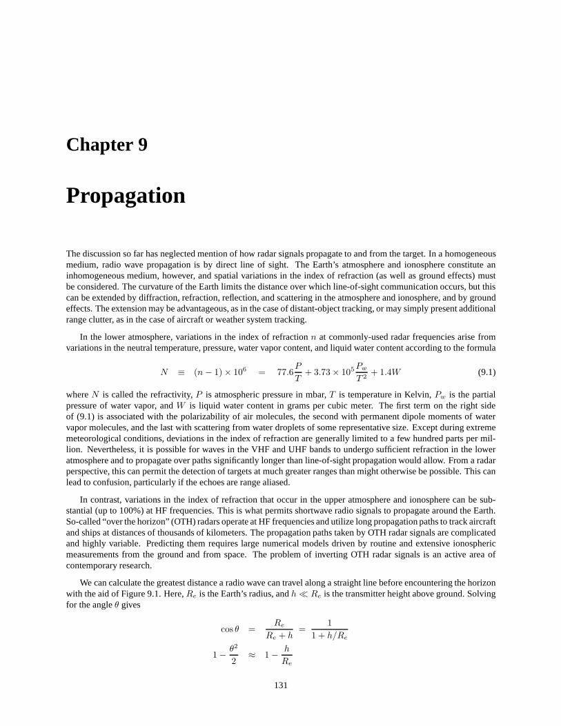
We can calculate the greatest distance a radio wave can travel along a straight line before encountering the horizonwith the aid of Figure 9.1. Here,Re is the Earth’s radius, andh≪ Re is the transmitter height above ground. Solvingfor the angleθ gives

cos θ =Re

Re + h=

1

1 + h/Re

1 − θ2

2≈ 1 − h

Re

131

Re

z=h

θ

ψ

z=0

z

n(z)

Figure 9.1: Radio wave propagation geometry. Two ray paths are shown: one along a straight path terminating at thehorizon, and the other along a refracted path. The latter must have a turning point (ψ = π/2) if the ray is to return tothe ground past the transmitter’s horizon.

or θ ≈√

2h/Re. The corresponding arc length on the ground isReθ =√

2Reh. For example, radio signals launchedfrom ah = 100 m tower will encounter the horizon at a distance of about 35 km. This is about the limit for FM radioand television signals, which propagate mainly by line of sight. The range can be extended by elevating the radio sourcefurther, as in the case of airborne radar (AWACS) which can beabout 100 times higher and have ten times the range ofground-based radar installations. Spaceborne radar can cover still greater range. The range of communications linkscan also be extended by incorporating high-altitude scatterers. Turbulent scatter in the troposphere and stratosphereand meteor scatter in the mesosphere and lower thermospherehave been utilized this way. Communications satelliteshave rendered these techniques largely obsolete, however.

9.1 Tropospheric ducting

The index of refraction in the Earth’s troposphere varies with altitude, mainly because of varying water vapor concen-tration, and radio waves propagate along curved lines as a result. This can greatly increase the distance radio signalstravel, particularly over water when meteorological conditions are favorable. Radio and television signals sometimespropagate across the Great Lakes and rarely across even larger bodies of water in so-called tropospheric ducts, whichfunction like weakly-guiding dielectric waveguides.

In a spherically stratified medium, Snell’s law applied along a radio ray path can be shown to take the form(Bouger’s law):

(Re + z)n(z) sinψ(z) = const (9.2)

wheren(z) is the index of refraction,z is the height above ground,ψ is the zenith angle shown in Figure 9.1, andthe radius of curvature of the dashed line isRe + z. After differentiation with respect toz and noting thatdz ≈cotψ(Re + z)dθ, we have

1

(Re + z)

dψ

dθ= −

(

1

n

dn

dz+

1

Re + z

)

(9.3)

where the term on the left is the rate of chage of zenith angle with lateral displacement and the trailing term in theparentheses on the right is a purely geometric effect associated with propagation over a spherical body. In order for

132

the ray to travel horizontally, exactly following the curvature of the Earth, we requiredψ/dθ = 0 and therefore

dn

dz= − n

Re + z≈ − 1

Re(9.4)

where we note again that the index of refraction is typicallynearly unity throughout the troposphere, differing myno more than a few hundred ppm. In fact, under standard atmospheric conditions,dn/dz ≈ −1/4Re. This meansthat the gradient in the index of refraction is usually insufficiently strong to maintain horizontal radio ray paths, thatdψ/dθ < 0, and that the radio waves will exhibit some curvature but ultimately escape into space.

Examining (9.3), we see that the rate of change of the wave zenith angle under standard atmospheric conditions isidentical to what it would be if there were no refraction and if the radius of the Earth wereae ≈ (4/3)Re. Consequently,the height of the ray above ground would be the same in either case. A common practice for incorporating the effectsof atmospheric refraction in propagation calculations is to assume straight-line propagation, only replacingRe withae. This has the minor effect of increasing the distance estimates from the previous section by a factor of

√

4/3.

When |n′(z)| is greater than (less than) about1/4Re, we have superstandard (substandard) refraction. If it isgreater than1/Re, ducting may occur, and radio waves can be refracted back to Earth. This can happen at ground level(a surface duct) or well above the surface (an elevated duct)during unusual meteorological conditions, particularly overwater. It can also occur where surface heating or other meteorological conditions create a temperature inversion withassociated effects on the refractivity profile. Surface ducts tend to be lossy because they incorporate scattering off theground, which sends radiation off in all directions. Elevated ducts act like dielectric wavegudes created by perturbedrefractivity layers at altitude. They can convey radiationefficiently over long distances, but coupling radiation into andout of them is difficult. How well confined a radio wave is to a duct and over what distance it can propagate dependsin the duct thickness and steepness (the refractivity gradient).

We can model an elevated duct as a thin layer where the index ofrefraction has a parabolic shape:

n(z) = n + n1z(h− z)(4/h2), 0 ≤ z ≤ h

wheren andn1 are the indices of refraction at the edges and the center of the duct, respectively. Let the radiusof curvature of the guided wave be sufficiently small when it is in the duct that we can neglect the Earth’s gradualcurvature by comparison. Suppose a wave is launched into themidpoint of the duct atz = h/2 and at an angleψi

with respect to the vertical. Snell’s law for a vertically stratified medium is justn sinψ = const or

n(z) sinψ = n(h/2) sinψi

At the turning points, the wave propagates horizontally, and n(z) = n(h/2) sinψi. Solving from the model, theheights of the turning points must be

z = zt =h

2

[

1 ±(

1 +n

n1

)1/2

(1 − sinψ)1/2

]

The question then is whether or not the turning points are inside the layer. If they are, the wave will remain within thewaveguide. Otherwise, it will penetrate the upper boundaryand escape. This happens if the initial zenith angle is toosteep. The critical angle is the initial zenith angle givinga turning point precisely atz = h, viz.

sinψc =1

1 + (n1/n)

For example, takingn = 1 andn1 = 1 × 10−4 (corresponding to a 100 ppm maximum perturbation in the index ofrefraction across the duct) gives the critical angleψc = 89.2, showing that waves must be launched nearly horizontallyto be ducted. This means that it is easier to couple radio waves into surface ducts than elevated ducts. Of those waveswith shallow enough zenith angles to be confined, only wave modes withλ < hwill actually be confined to and guidedby the waveguide, and only those withλ ≪ h are likely to be remain confined over long distances. Perturbations inthe index of refraction caused by water vapor are most significant for waves in the microwave band, but these also tendto suffer the most absorption. In practice, waves in the VHF and UHF bands are the most prone to ducting.

133

109 1010 1011 1012

Ne (m-3)

Alt(km)

50

100

500

1000

DE

F1

F2

E

F

night day

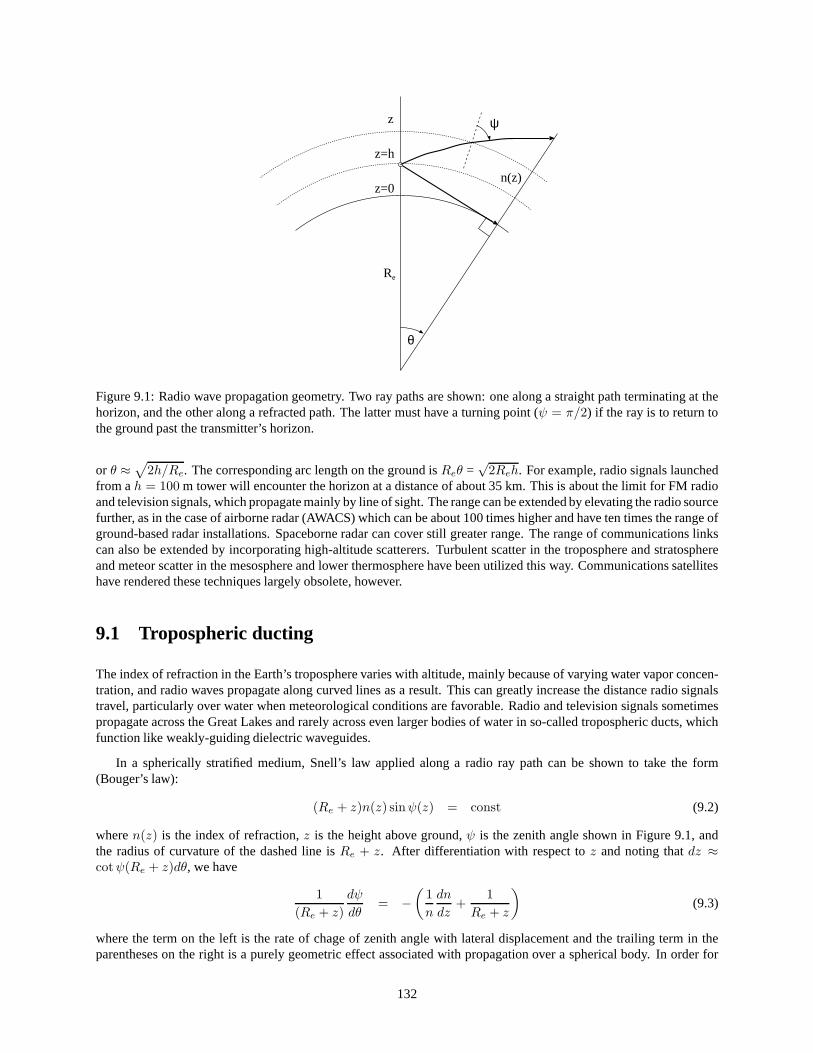
Figure 9.2: Electron number density in the Earth’s ionosphere.

9.2 Ionospheric refraction

Radio waves are often sorted into one of three categories: ground waves, space waves, and sky waves. Ground wavesare guided by the dielectric waveguide formed at the air/ground interface. This is a rather lossy waveguide, and onlylow-frequency waves can propagate long distances without severe attenuation. Low-frequency signals, including AMradio signals, can propagate several tens of kilometers this way, permitting reception even after the transmitting towerfalls below the horizon.

VHF and higher frequency waves (along with HF waves launchedat high elevation angles) propagate along almoststraight lines into space and are known as space waves. HF andlower frequency waves meanwhile are refracted asthey pass through the Earth’s ionosphere, a layer of the upper atmosphere that is partially ionized and that representsa population of free electrons. Whereas the index of refraction is only perturbed slightly in atmospheric ducts, it canvary drastically in the ionosphere. If both the radio wave frequency and elevation angle are low enough, signals canreturn along wide arcs to ground level at great distances (over the horizon) from their origin. These are sky waves. Thegap where neither ground waves nor sky waves are detected is called theskip distance. At sufficiently low frequencies,ionospheric refraction becomes reflection, the wide arcs become sharp angles, and there is no skip distance.

Roughly speaking, waves between 10–40 MHz can propagate long distances via ionospheric refraction, whereaswaves between 2–10 MHz can do so via ionospheric reflection. Below about 2 MHz, strong absorption in the lowestlayer of the ionosphere (the D region) prohibits long distance propagation during the day, but reflection still occurs atnight. This phenomenon is easily detected by listening to AMradio.

Figure 9.2 shows representative daytime and nighttime electron density profiles for the Earth’s ionosphere. Actualprofiles vary with location, local time, season, and solar cycle. There are three main ionospheric layers, the D,E, and F layers. These layers are generated by photoionization from solar radiation and shaped by chemical anddynamical (winds, electric fields) processes. Above the F layer, the neutral atmosphere is too tenuous for significantphotoionization to occur. Below the D layer, meanwhile, most of the ionizing radiation from the sun has been absorbed.The E layer (“E” stands for electric) was discovered first because of the strong electric currents that flow in it. TheF layer is the densest and is associated with long-distance radio wave propagation. During the day, it splits subtlyinto two layers (although the F1 layer is really more of a ledge.) The D layer exists only during the day. Collisionswith the dense neutral atmosphere cause this layer to be verylossy, and radio signals that interact with it are stronglyattenuated. At night, chemical recombination removes muchof the lower ionosphere, but the upper ionosphere losesonly some of its ionization.

The ionosphere is everywhere very nearly charge neutral, with electrons and ions occurring in close proximity.

134

Electrons and ions respond differently to electric fields, however, and so conduction current can flow. Conductioncurrent combines with displacement current and modifies theindex of refraction of the medium, causing radio wavesto reflect, refract, and exhibit other interesting and important phenomena.

Some of these phenomena can be understood my modeling the ionosphere as a uniform background of ions whichare relatively massive and fixed, with an equal number of relatively mobile electrons intermixed. We will neglect theEarth’s magnetic fieldB for the moment, although this will turn out to be important, as we will see in section 9.4 Theelectrons obey Newton’s second law:

medv

dt= −eE−meνv

Reading from left to right, the terms in this equation for theelectron momentum represent inertia, the Coulomb force,and collisional drag, withν representing the collision rate with neutral species. Applying phasor notation and solvingfor the electron velocity yields:

v =−eE

(jω + ν)me

whereω is the frequency of the electric field applying force to the electrons. Notice that the electron drift is generallyout of phase with the applied Coulomb force because of the effect of inertia. Associated with this electron drift is acurrent densityJ = −Neev, whereNe is the number density of electrons. This current is also out of phase with theelectric field. The current can be incorporated into Ampere’s law:

∇× H = J + iωǫE

= iωǫE

ǫ(ω) ≡ ǫ

(

1 − e2Ne/ǫme

ω(ω − jν)

)

Notice how the conduction current has been absorbed into an effective, frequency-dependent dielectric constantǫ(ω).This redefinition of the dielectric constant affords a simple means of assessing the effect of currents in a plasma onradio wave propagation, since the index of refraction in a dielectric is defined byn2 ≡ ǫ/ǫ. A plasma is not a dielectricper se, since it has mobile charge carriers, but the analogy is a powerful and useful one.

Plasmas exhibit a characteristic resonance frequency called theplasma frequency

ωp = 2πfp =

√

e2Ne

ǫme

fp ≈ 9√

Ne (MKS units)

which corresponds to the natural oscillation frequency of the electrons with finite inertia and a Coulomb restoringforce. The index of refraction for electromagnetic waves inan unmagnetized plasma is then given by

n2 = 1 −ω2

p

ω(ω − jν)(9.5)

≈ 1 −ω2

p

ω2, ν ≪ ω

When the wave frequency is comparable to both the plasma frequency and the collision frequency, the index of refrac-tion has a significant imaginary component, and attenuationoccurs. This happens to MF (medium frequency) wavesduring the daytime. In the collisionless limit, when the wave frequency is less than the plasma frequency, the index ofrefraction becomes imaginary, and wave propagation ceases. Radio waves reflect at altitudes where this occurs. Sincethe peak plasma number density is seldom much greater than1×1012 m−3, reflection is usually limited to frequenciesbelow about 10 MHz. (The plasma frequency associated with the plasma density at the F layer peak is called thecrit-ical frequency fc, which is the highest reflection frequency.) Finally, the index of refraction can depart significantlyfrom unity even when the wave frequency is above the plasma frequency. This is the regime of ionospheric refraction.Note that, forν ≪ ω, ωp plays the same role as the cutoff frequency for waves propagating in a waveguide. In thatway, the plasma can act like a high-pass filter.

135

Re

θ

dmax

h’

ψi

Figure 9.3: Radio wave propagation at the MUF.

9.2.1 Maximum usable frequency (MUF)

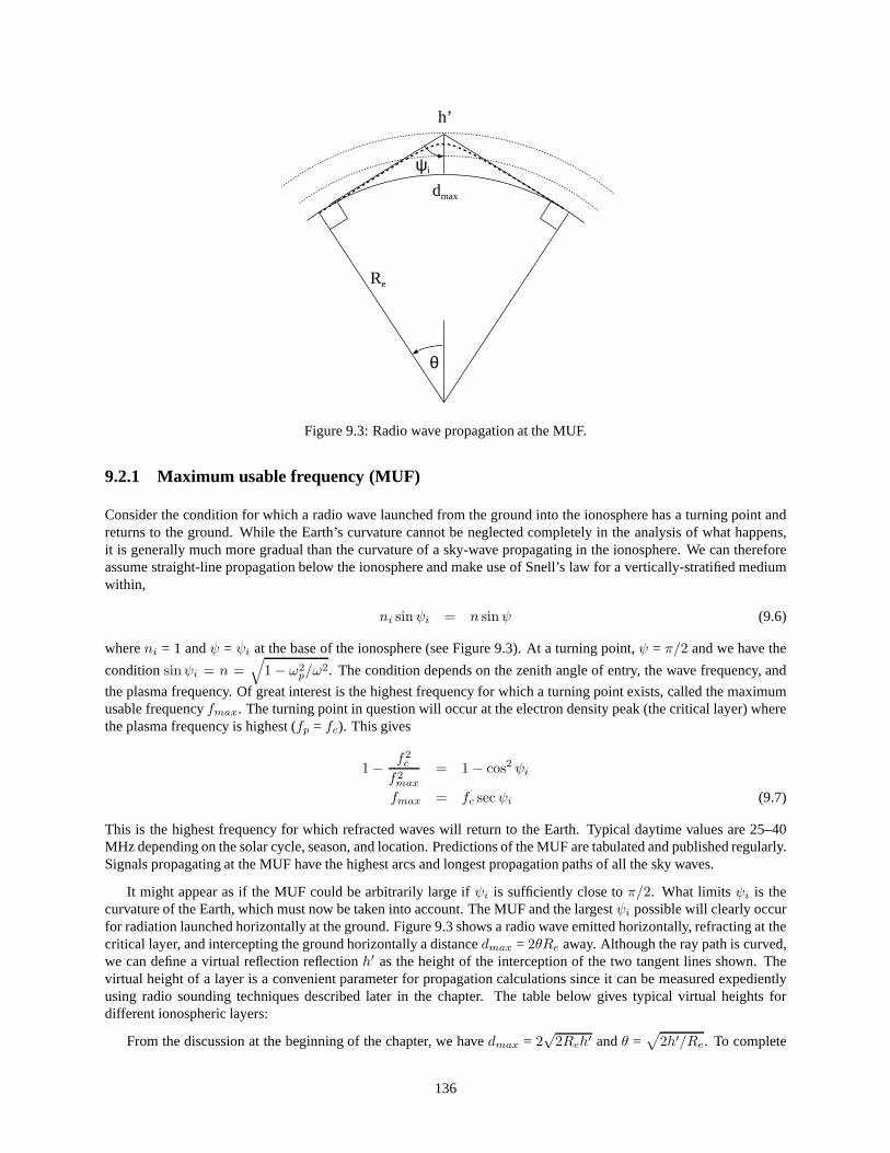
Consider the condition for which a radio wave launched from the ground into the ionosphere has a turning point andreturns to the ground. While the Earth’s curvature cannot beneglected completely in the analysis of what happens,it is generally much more gradual than the curvature of a sky-wave propagating in the ionosphere. We can thereforeassume straight-line propagation below the ionosphere andmake use of Snell’s law for a vertically-stratified mediumwithin,

ni sinψi = n sinψ (9.6)

whereni = 1 andψ = ψi at the base of the ionosphere (see Figure 9.3). At a turning point, ψ = π/2 and we have the

conditionsinψi = n =√

1 − ω2p/ω

2. The condition depends on the zenith angle of entry, the wavefrequency, and

the plasma frequency. Of great interest is the highest frequency for which a turning point exists, called the maximumusable frequencyfmax. The turning point in question will occur at the electron density peak (the critical layer) wherethe plasma frequency is highest (fp = fc). This gives

1 − f2c

f2max

= 1 − cos2 ψi

fmax = fc secψi (9.7)

This is the highest frequency for which refracted waves willreturn to the Earth. Typical daytime values are 25–40MHz depending on the solar cycle, season, and location. Predictions of the MUF are tabulated and published regularly.Signals propagating at the MUF have the highest arcs and longest propagation paths of all the sky waves.

It might appear as if the MUF could be arbitrarily large ifψi is sufficiently close toπ/2. What limitsψi is thecurvature of the Earth, which must now be taken into account.The MUF and the largestψi possible will clearly occurfor radiation launched horizontally at the ground. Figure 9.3 shows a radio wave emitted horizontally, refracting at thecritical layer, and intercepting the ground horizontally adistancedmax = 2θRe away. Although the ray path is curved,we can define a virtual reflection reflectionh′ as the height of the interception of the two tangent lines shown. Thevirtual height of a layer is a convenient parameter for propagation calculations since it can be measured expedientlyusing radio sounding techniques described later in the chapter. The table below gives typical virtual heights fordifferent ionospheric layers:

From the discussion at the beginning of the chapter, we havedmax = 2√

2Reh′ andθ =√

2h′/Re. To complete

136

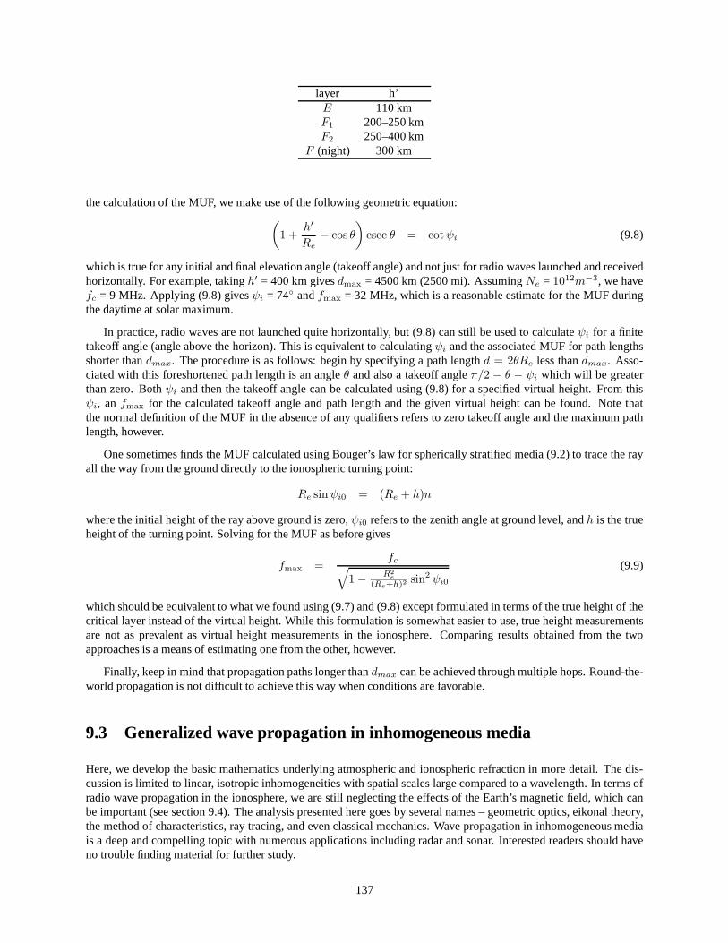
layer h’E 110 kmF1 200–250 kmF2 250–400 km

F (night) 300 km

the calculation of the MUF, we make use of the following geometric equation:(

1 +h′

Re− cos θ

)

csec θ = cotψi (9.8)

which is true for any initial and final elevation angle (takeoff angle) and not just for radio waves launched and receivedhorizontally. For example, takingh′ = 400 km givesdmax = 4500 km (2500 mi). AssumingNe = 1012m−3, we havefc = 9 MHz. Applying (9.8) givesψi = 74 andfmax = 32 MHz, which is a reasonable estimate for the MUF duringthe daytime at solar maximum.

In practice, radio waves are not launched quite horizontally, but (9.8) can still be used to calculateψi for a finitetakeoff angle (angle above the horizon). This is equivalentto calculatingψi and the associated MUF for path lengthsshorter thandmax. The procedure is as follows: begin by specifying a path length d = 2θRe less thandmax. Asso-ciated with this foreshortened path length is an angleθ and also a takeoff angleπ/2 − θ − ψi which will be greaterthan zero. Bothψi and then the takeoff angle can be calculated using (9.8) for aspecified virtual height. From thisψi, an fmax for the calculated takeoff angle and path length and the given virtual height can be found. Note thatthe normal definition of the MUF in the absence of any qualifiers refers to zero takeoff angle and the maximum pathlength, however.

One sometimes finds the MUF calculated using Bouger’s law forspherically stratified media (9.2) to trace the rayall the way from the ground directly to the ionospheric turning point:

Re sinψi0 = (Re + h)n

where the initial height of the ray above ground is zero,ψi0 refers to the zenith angle at ground level, andh is the trueheight of the turning point. Solving for the MUF as before gives

fmax =fc

√

1 − R2e

(Re+h)2 sin2 ψi0

(9.9)

which should be equivalent to what we found using (9.7) and (9.8) except formulated in terms of the true height of thecritical layer instead of the virtual height. While this formulation is somewhat easier to use, true height measurementsare not as prevalent as virtual height measurements in the ionosphere. Comparing results obtained from the twoapproaches is a means of estimating one from the other, however.

Finally, keep in mind that propagation paths longer thandmax can be achieved through multiple hops. Round-the-world propagation is not difficult to achieve this way when conditions are favorable.

9.3 Generalized wave propagation in inhomogeneous media

Here, we develop the basic mathematics underlying atmospheric and ionospheric refraction in more detail. The dis-cussion is limited to linear, isotropic inhomogeneities with spatial scales large compared to a wavelength. In terms ofradio wave propagation in the ionosphere, we are still neglecting the effects of the Earth’s magnetic field, which canbe important (see section 9.4). The analysis presented heregoes by several names – geometric optics, eikonal theory,the method of characteristics, ray tracing, and even classical mechanics. Wave propagation in inhomogeneous mediais a deep and compelling topic with numerous applications including radar and sonar. Interested readers should haveno trouble finding material for further study.

137

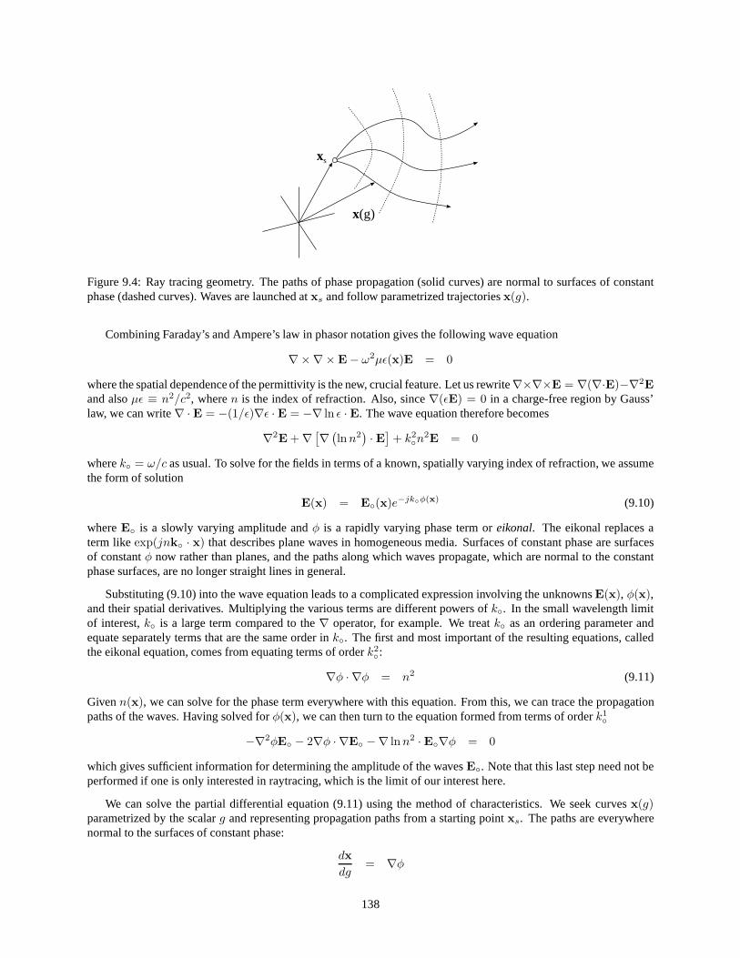
xs

x(g)

Figure 9.4: Ray tracing geometry. The paths of phase propagation (solid curves) are normal to surfaces of constantphase (dashed curves). Waves are launched atxs and follow parametrized trajectoriesx(g).

Combining Faraday’s and Ampere’s law in phasor notation gives the following wave equation

∇×∇× E− ω2µǫ(x)E = 0

where the spatial dependence of the permittivity is the new,crucial feature. Let us rewrite∇×∇×E = ∇(∇·E)−∇2E

and alsoµǫ ≡ n2/c2, wheren is the index of refraction. Also, since∇(ǫE) = 0 in a charge-free region by Gauss’law, we can write∇ · E = −(1/ǫ)∇ǫ · E = −∇ ln ǫ · E. The wave equation therefore becomes

∇2E + ∇

[

∇(

lnn2)

· E]

+ k2n

2E = 0

wherek = ω/c as usual. To solve for the fields in terms of a known, spatiallyvarying index of refraction, we assumethe form of solution

E(x) = E(x)e−jkφ(x) (9.10)

whereE is a slowly varying amplitude andφ is a rapidly varying phase term oreikonal. The eikonal replaces aterm likeexp(jnk · x) that describes plane waves in homogeneous media. Surfaces of constant phase are surfacesof constantφ now rather than planes, and the paths along which waves propagate, which are normal to the constantphase surfaces, are no longer straight lines in general.

Substituting (9.10) into the wave equation leads to a complicated expression involving the unknownsE(x), φ(x),and their spatial derivatives. Multiplying the various terms are different powers ofk. In the small wavelength limitof interest,k is a large term compared to the∇ operator, for example. We treatk as an ordering parameter andequate separately terms that are the same order ink. The first and most important of the resulting equations, calledthe eikonal equation, comes from equating terms of orderk2

:

∇φ · ∇φ = n2 (9.11)

Givenn(x), we can solve for the phase term everywhere with this equation. From this, we can trace the propagationpaths of the waves. Having solved forφ(x), we can then turn to the equation formed from terms of orderk1

−∇2φE − 2∇φ · ∇E −∇ lnn2 · E∇φ = 0

which gives sufficient information for determining the amplitude of the wavesE. Note that this last step need not beperformed if one is only interested in raytracing, which is the limit of our interest here.

We can solve the partial differential equation (9.11) usingthe method of characteristics. We seek curvesx(g)parametrized by the scalarg and representing propagation paths from a starting pointxs. The paths are everywherenormal to the surfaces of constant phase:

dx

dg= ∇φ

138

According to (9.11), we then have

dx

dg· dxdg

= n2 (9.12)

Differentiating with respect tog yields

d2x

dg2= n∇n (9.13)

What was once a PDE has become three uncoupled, 2nd order, scalar ODEs, one for each vector component ofx(g).Note also the form of the equations. With the appropriate scaling, (9.13) has the form of Newton’s second law, withthen∇n term playing the role of a generalized force. Ray paths evidently follow ballistic trajectories, and solutionsto (9.13) can be highly intuitive as a result. Of course, the path depends on the initial conditions as well as onn, justas the initial position and velocity of a ballistic object, together with the applied force, determine its trajectory.

What isg? It is related to path length, but what is the relationship? Note that, by definition, one may always write

dx

ds· dxds

= 1

whereds2 = dx2 +dy2 +dz2 andds is a physical path length element. Comparing with (9.12) shows thatds/dg = n,or thatdg is linearly related tods by the index of refraction. We callg the optical path length, which is proportional tothe path length measured in wavelengths rather than fixed units.

9.3.1 Stratified media

Consider what happens to (9.13) in vertically stratified media. In the horizontal (x) direction, we have

d2x

dg2=

d

dg

(

dx

dg

)

= nd

ds

(

ndx

ds

)

= 0

Integrating yields

n(z)dx

ds= c

wherec is a constant of integration. If the zenith angle of the ray atany instant isθ, thendx/ds is justsin θ, meaning

n(z) sin θ = c = sin θ (9.14)

where we take the index of refraction to be unity at the originof the ray path, whereθ = θ. Equation (9.14) is ofcourse just Snell’s law in a stratified medium. While this is sufficient information to trace the ray, we can develop anexplicit equation for the ray trajectory by manipulating the vertical(z) component of (9.13):

nd

ds

(

ndz

ds

)

= ndn

dz=

1

2

d(n2)

dz

To this, we apply Snell’s law in the formds = (n/c)dx to find

d2z

dx2=

1

2c2d

dz(n2)

Note further that, along a line segment,d/dx = (dz/dx)d/dz. Therefore, the left side of the preceding equation is(dz/dx)d/dz(dz/dx) or

1

2

d

dz

(

dz

dx

)2

=1

2c2d

dz(n2)

139

Integrating once inz gives

(

cdz

dx

)2

= n2(z) +B

whereB is another constant of integration. Recalling that we have takenn(0) = 1 and thatc = sin θ as a consequenceallows the assignmentB = − sin2 θ (sincedz/dx at the origin iscot θ). Taking the reciprocal of the square root ofthe resulting equation and integrating then gives the desired equation for the ray trajectory:

x(z) =

∫ z

0

√

sin2 θ

n2(z) − sin2 θdz

In a homogeneous medium withn = 1, this obviously gives the equation for a straight line,x = z tan θ. In inhomo-geneous media, it specifies a ray which may or may not return tothez = 0 interface, depending on the steepness of theindex of refraction gradient and the initial zenith angleθ.

9.3.2 Radius of curvature

It is often useful to formulate the raytracing problem in curvilinear coordinates, as in the case of a ray bent into anearly circular arc. Care must be taken here since the coordinate axes themselves vary with position. Returning to theballistic equation, we have

d2x

dg2= n∇n with

ds

dg= n

nd

ds

(

ndx

ds

)

= n∇n

In polar coordinates,x = rer andds = rdθ on a circular arc. Furthermore,der/dθ = eθ anddeθ/dθ = −er. Alltogether,

d

ds(neθ) = ∇n

dn

dseθ −

n

rer = ∇n

wherer has been held constant throughout. Taking the dot product with er then gives

1

r= −∇ lnn · er

which relates the radial gradient in the index of diffraction to the radius of curvature of a refracted ray. For example,we can determine how the index of refraction must vary in order for the ray to be bent into a circular arc of radiusRe.

− dr

Re= d lnn

− r

Re+ C = lnn

n = ne−r/Re

This shows that the radius of curvature of a circular ray is the scale height of the index of refraction in a radiallystratified medium, in agreement with statements made earlier. Note that the calculations become more cumbersome ifdeviations from a circular path are allowed.

140

9.4 Birefringence (double refraction)

Reflection and refraction are hallmarks of radio wave propagation in inhomogeneous media. Birefringence, mean-while, is an additional effect characteristic of waves propagating in anisotropic media. An anisotropic medium is onethat responds differently depending on the direction of forcing. Many crystals have this property because of asymme-tries in their lattice structure. In the ionosphere, anisotropy arises from the Earth’s magnetic field and the effect of theJ×B component of the Lorentz force on the currents driven by electromagnetic waves. This effect has been neglectedso far but is quite important for understanding ionosphericradio wave propagation.

Mathematically, the dielectric constant in an anisotropicmedium is generally described by a matrix rather than asingle constant. The consequence of this is that the equation governing the index of refraction is quadratic and has twoviable solutions or modes. Two distinct kinds of waves may therefore propagate in any given direction in the medium.The two generally obey different dispersion relations and have different polarizations. When the two interfere, thepolarization of the combined wave can vary in ways not observed in isotropic media.

Let us return to Newton’s second law, this time including theJ× B component of the Lorentz force:

medv

dt= −e(E + v × B) −meνv

In this equation,B denotes the Earth’s background magnetic field and not the magnetic field due to the wave itself,which exerts negligible force on electrons moving at non-relativistic speeds. This equation can be solved for theelectron velocity, which is linearly related to the wave electric field, but the relationship is through a matrix, calledthemobility matrix. Its form is simplified by working in Cartesian coordinates and taking the Earth’s magnetic field to liein the z direction:

vx

vy

vz

=

µ11 µ12

µ21 µ22

µ33

Ex

Ey

Ez

µ11 = µ22 = −(

1 +(jω + ν)2

Ω2e

)−1jω + ν

ΩeB

µ12 = −µ21 =

(

1 +(jω + ν)2

Ω2e

)−11

B

µ33 = − Ωe/B

jω + ν

The termΩe = eB/me is the angular electron gyrofrequency which gives the angular frequency of gyration of theelectrons around the Earth’s magnetic field lines. Anisotropy results from the fact that electrons are bound to orbitsaround magnetic field lines but are relatively free to move along the field lines. In the ionosphere,Ωe/2π ≤ 1.4 MHzand depends on magnetic latitude and altitude. Theµ33 term is what would be found in an isotropic plasma with nobackground magnetic field. As the wave frequency increases well beyond the gyrofrequency,µ11 andµ22 approachµ33, and the off-diagonal terms of the mobility matrix become small. Nevertheless, so-called magneto-ionic effectsremain significant even at radio frequencies much higher than Ωe/2π.

The current density is related to the electron drift velocity by J = −Neev, and to the electric field by the consti-tutive relationshipJ = σE, whereσ is the conductivity matrix. For wave frequencies much greater than the electrongyrofrequency and collision frequency, the nonzero elements of the conductivity matrix are:

σ11 = σ22 = Nee

(

1 − ω2

Ω2e

)−1jω

ΩeB

σ12 = −σ21 = −Nee

(

1 − ω2

Ω2e

)−11

B

σ33 = −jNeeΩe/B

ω

141

Finally, we can write Ampere’s law once again as:

∇× H = J + iωǫE

= (σ + iωǫI)E

= iωǫE

ǫ =

ǫ11 ǫ12ǫ21 ǫ22

ǫ33

ǫ11 = ǫ22 = ǫ

(

1 +ω2

p

Ω2e − ω2

)

ǫ12 = −ǫ21 = jǫΩe

ω

ω2p

Ω2e − ω2

ǫ33 = ǫ

(

1 −ω2

p

ω2

)

The dielectric matrix gives a description of the response ofthe medium, the ionospheric plasma in this case,to electromagnetic waves. In effect, the dielectric matrixgives the electrical displacement that arises from electricfields applied in different directions. Obviously, the displacement is not parallel to the electric field in general. Thishas important implications, including the fact that the phase velocity of the waves (which is normal to the electricaldisplacement – see below) and the group velocity (which is parallel to the Poynting flux and therefore normal tothe electric field) need not be parallel. Waves propagating in the same direction but with different polarizations willmoreover be governed by different components of the dielectric matrix and so will behave fundamentally differently,having different phase and group velocities, for example, and different reflection conditions.

9.4.1 Fresnel equation of wave normals

To analyze the behavior of electromagnetic waves in the plasma, we combine Faraday’s law and Ampere’s law inmacroscopic form. We seek plane-wave solutions for the fieldquantities of the formexp j(ωt − k · r). In phasornotation, Faraday’s and Ampere’s law in a charge-free, current-free region become:

k × E = ωµH

k × B = −ωD

These equations apply to the ionospheric plasma, which is charge-neutral (ions and electrons everywhere in approxi-mately equal density) so long as the conduction current is included in the definition of the dielectric constant and theelectric displacement. From the above equations, we can conclude that the wavevectork will be normal both to themagnetic field/magnetic induction and also to the electric displacement but not necessarily to the electric field.

Combining Maxwell’s equations yields the desired wave equation:

k(k ·E) − k2E + ω2µǫ · E = 0

where the dielectric constant is the matrix derived just above. In matrix form, the wave equation can be expressed as

ω2µǫ11 − k2 + k2x ω2µǫ12 + kxky kxkz

ω2µǫ21 + kxky ω2µǫ22 − k2 + k2y kykz

kxkz kykz ω2µǫ33 − k2 + k2z

Ex

Ey

Ez

= 0

142

For a given wave frequencyω, the objective now is to solve the above for the wavevectork(ω), which constitutes adispersion relation. If a solution other than the trivial solution (Ex, Ey, Ez = 0) is to exist, the 3x3 matrix above mustbe singular and therefore non-invertible. We therefore findthe dispersion relation by setting the determinant of thematrix equal to zero. The resulting equation is called the wave normal equation.

Having found one or more wavevectors that solve the wave normal equation, we can then substitute them backinto the 3x3 matrix to see what they imply aboutE. There is no unique solution for the electric field amplitudecorresponding to each wavevector found, since any solutionmultiplied by a constant remains a solution. However,it is possible to find the ratio of the componentsEx : Ey : Ez corresponding to each solution or mode. This ratiodetermines the polarization of the given mode.

A convenient way to express the dispersion relation is by solving for the wavenumberk as a function of thefrequencyω and the prescribed phase propagation directionk = k/k. Since the problem is azimuthally symmetricabout the magnetic field, the direction can be expressed wholly in terms of the angleθ between the magnetic field andthe wavevector,θ. Finally, it is common to write the dispersion relation in terms of the index of refraction, which isrelated to the wavenumber byn2 = c2k2/ω2. Consequently, we will solve the wave normal equation forn(ω, θ).

The wave normal equation is quadratic inn2, and so we expect two independent solutions for any given wavefrequency and propagation direction. (The word “birefringence” refers to the dual solutions.) These are the so-calledmagneto-ionic modes of propagation. The two modes will havedistinct, orthogonal polarizations and be governed bydifferent dispersion relations. Radiation launched into the ionosphere at arbitrary direction and polarization willdivideinto two modes which may then depart from one another. In general, superimposed modes will exhibit a combinedpolarization that varies in space.

9.4.2 Astrom’s equation

Considerable effort has been invested in finding compact ways of writing the wave normal equation for an ionosphericplasma. One of these is

(

n21

n2 − n21

+n2−1

n2 − n2−1

)

sin2 θ

2+

n2

n2 − n2

cos2 θ = 0

n2α ≡ 1 − X

1 − αY, α = −1, 0, 1

X ≡ ω2p/ω

2

Y ≡ Ωe/ω

Here,ω andθ are independent variables, andn2 is the dependent variable. The other variables are auxiliary variables;α takes on values from -1 to 1 inclusive.

9.4.3 Booker quartic

An equivalent formulation is found by multiplying Astrom’sequation to clear the fractions:

[

n21(n

2 − n2−1) + n2

−1(n2 − n2

1)] sin2 θ

2+ n2

(n2 − n2

1)(n2 − n2

−1) cos2 θ = 0

In this formulation, the wave normal equation is clearly quadratic inn2.

143

0.5 1 1.5 2X

-2

-1.5

-1

-0.5

0.5

1

1.5

2n2

0.5 1 1.5 2X

-2

-1.5

-1

-0.5

0.5

1

1.5

2n2

0.5 1 1.5 2X

-2

-1.5

-1

-0.5

0.5

1

1.5

2n2

0.5 1 1.5 2X

-2

-1.5

-1

-0.5

0.5

1

1.5

2n2

0.5 1 1.5 2X

-2

-1.5

-1

-0.5

0.5

1

1.5

2n2

θ = π/2 θ=π/4 θ=π/8

θ=π/20 θ=0

XO

X

Figure 9.5: Dispersion curves plotted for various propagation anglesθ. In each plot, the horizontal and vertical axesrepresentX=ω2

p/ω2 andn2, respectively. Curves are plotted for the conditionY =

√X/3 (meaningΩe = ωp/3).

Note that the range of frequencies plotted here excludes thelow-frequencyY > 1 region where additional interestingbehavior can be found.

9.4.4 Appleton-Hartree equation

By factoring the Booker quartic, one can obtain the Appleton-Hartree equation:

n2 = 1 − X

1 − Y 2

T

2(1−X) ±√

Y 4

T

4(1−X)2 + Y 2L

where

YT ≡ Y sin θ

YL ≡ Y cos θ

The termsYT andYL refer to transverse and longitudinal propagation with respect to the background magneticfield. In the quasi-transverse and quasi-longitudinal limits, one term is deemed negligible compared to the other.

The three equivalent equations may seem daunting, but a little inspection yields incisive information. The conditionfor wave propagation isn2 > 0. In the eventn2 < 0, the wave is evanescent. Settingn2 = 0 in the Booker quarticyields an equation for the cutoff frequencies:

n2n

21n

2−1 = 0

for all propagation angles with respect to the magnetic field. Settingn2 = 0 gives the conditionω2 = ω2

p. This isthe same cutoff condition as for waves in an isotropic plasma(no magnetic field), and so this is referred to as the“ordinary” mode cutoff. Settingn2

±1 = 0 meanwhile gives the conditionsX = 1 ∓ Y or ω2p = ω(ω ∓ Ωe). This

behavior is new, and so the frequencies are known as the “extraordinary” mode cutoffs. The terms “ordinary” and“extraordinary” actually come from crystalogrophy, wheresimilar ideas and terminology apply.

The dispersion relations contained within the three equations can be understood better by examining some illustra-tive limits. Consider first the case of propagation perpendicular to the magnetic fieldθ = π/2. In this limit, YT = Y ,YL = 0, and the two solutions to the Appleton Hartree equation are

n2 = 1 −X

144

n2 = 1 − X

1 − Y 2/(1 −X)

The first of these is identical to the dispersion relation in aplasma with no background magnetic field. There is acutoff atX = 1 or ω = ωp, and waves with frequencies above (below) the cutoff are propagating (evanescent). Sucha wave is called an ordinary or O-mode wave because of its similarity to waves studied in the simpler case of isotropicplasmas. It can be shown to have a characteristic linear polarization with an electric field parallel to the axis of thebackground magnetic field. Electrons accelerated by the wave electric field will experience nov×B force, and so themagnetic field has no effect on this wave.

The other solution is called the extraordinary or X-mode wave. This wave is also linearly polarized, but with theelectric field perpendicular to the background magnetic field. This wave has a resonance (n2 → ∞) atX=1 − Y 2

which is called the upper-hybrid resonance (hybrid since the resonant frequency involves both the plasma and theelectron cyclotron frequency). The wave propagates at highfrequencies and also at frequencies just below the upperhybrid frequency. It is evanescent at low frequencies and atfrequencies just above the upper hybrid frequency.

Figure 9.5 plots the dispersion relations for theθ = π/2 case for both the X- and O-mode waves. It also plotssolutions for other propagation angles. Similar features are found at all intermediate angles betweenθ = π/2 andθ = 0. These include an O-mode cutoff atX = 1 and an X-mode resonance at the upper hybrid frequency, givengenerally byX = (1−Y 2)/(1−Y 2

L). We have already determined that the X-mode cutoff frequencies are given byX= 1±Y for all propagation angles. What changes between the plots is the steepness of the curves near the upper-hybridresonance, where all the waves are clearly very dispersive.

The characteristic polarizations of the X- and O-modes are elliptical. For k · B > 0, the modes are right andleft elliptically polarized, respectively. As the propagation becomes close to parallel, the polarizations become nearlycircular. Since electrons orbit the magnetic field line in a right circular sense, the X-mode interacts more strongly withthe electrons, explaining the fact that it is more dispersive than the O-mode.

Another special limiting case is that of parallel propagation with θ = 0. Here, the upper-hybrid resonance and theX = 1 cutoff vanish, and the X- and O-modes coalesce into two modeswith cutoff frequencies still given byX =1 ± Y . From the Appleton Hartree equation, we find the dispersion relations for the two modes to be

n2 = 1 − X

1 ± Y

Whenk ·B > 0, the+/− solutions correspond, respectively, to left- and right-circularly polarized modes.

The vertical line atX = 1 reflects a resonance at the plasma frequency for parallel propagating waves. The wavesin question are non-propagating electrostatic plasma oscillations. The electric field for these waves is parallel to thewavevector and therefore parallel to the magnetic field, andthe electrons it accelerates do not experience aJ × B

force.

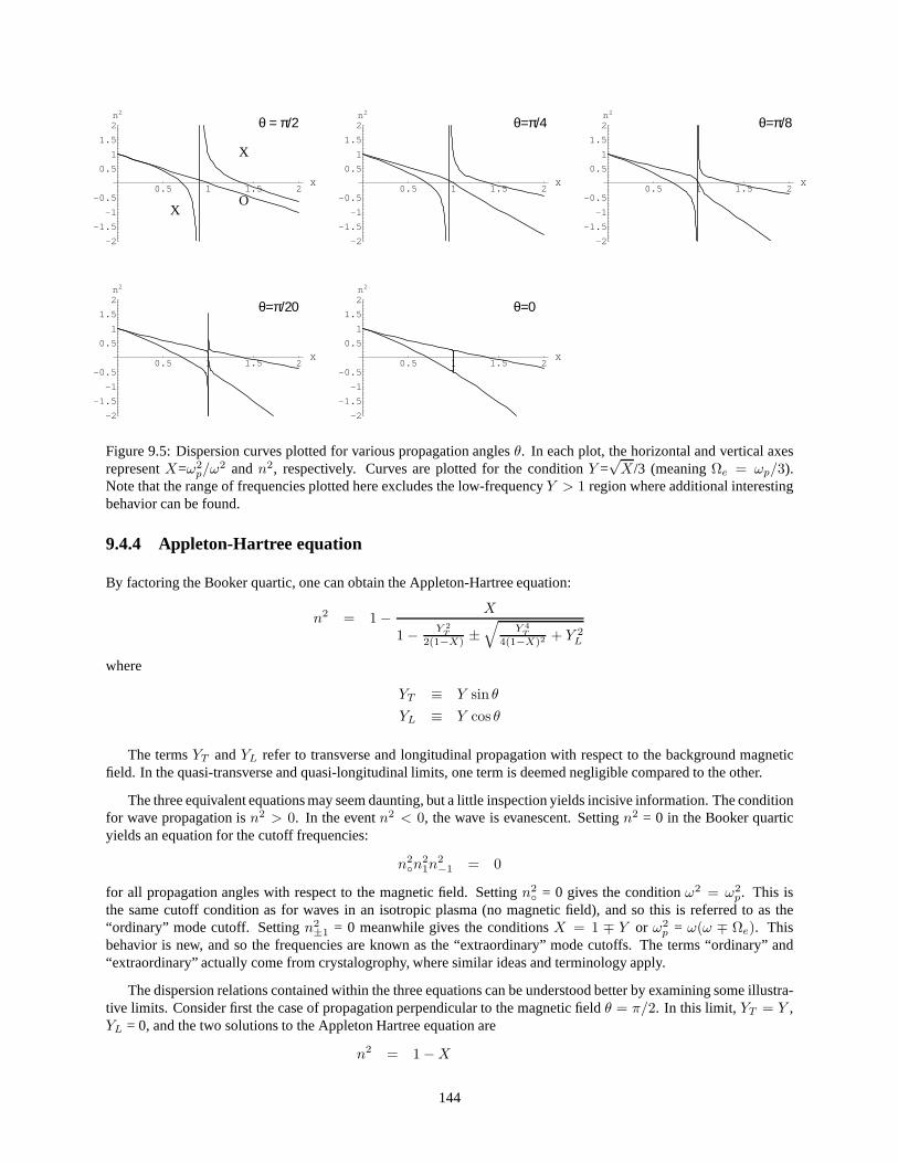
Figure 9.6 summarizes the findings so far. It is similar to Figure 9.5 except that 1) it is plotted on a log-log scale,2) it extends to largerX (lower frequency), and 3) it only shows propagating modes. Furthermore, curves for bothθ = 0 andθ = π/2 are plotted simultaneously. Waves propagating at arbitrary, intermediate angles can be thought ofas filling in the regions between these two extreme limits. Inspection of the figure reveals that, at any given frequencyand angle, there are two, one, or no propagating solutions.

At high frequency (X < 1), waves can propagate in one of two envelopes collectively referred to as the X andO modes, depending on which of these they approach in the perpendicular limit. Both have indices of refraction thatapproach unity asX = ω2

p/ω2 approaches zero and the plasma frequency becomes negligible compared to the wave

frequency. As the variableX increases, the X-mode cuts off first, followed by the O-mode.At frequencies belowthe plasma frequency (X > 1), wave propagation may take place in the so-called Z-mode. The cutoff frequenciesfor these three modes are the same three given above and do notdepend on propagation angle. The characteristicpolarization of the X- and O-mode waves are right- and left-elliptically polarized.

For waves propagating along the magnetic field, another resonance near the electron gyrofrequency (Y = 1) occursat still lower frequencies. This solution is also shown at the right side of Figure 9.6 forθ = 0. Waves propagating in thisbranch of the dispersion relation are highly dispersive andhave a group speed which increases with frequency. Pulses

145

0.5 1 5 10X

0.51

510

50100

n2

X

OZ

Figure 9.6: Summary of dispersion relations for all modes and propagation angles. Once again,Y =√X/3 here. A

qualitatively different set of curves results ifY >√X or Ω > ωp.

propagating in this mode will disperse in such a way that their high-frequency components arrive at their destinationfirst, followed by the low-frequency components. Radiationfrom lightning strikes can couple into this mode, givingrise to signals in the audible range with a characteristic whistling noise. Such waves are referred to as “whistlers.”

9.4.5 Phase and group velocity

As mentioned previously, a remarkable property of birefringent media is that the wave phase and group velocities candiffer not just in magnitude but also in direction. The phasevelocity is, by definition, in the direction of the wavevectorwhich is normal to the direction of the electric displacement. The group velocity, meanwhile, is in the direction of thePoynting flux, which is normal to the direction of the electric field. The electric displacement and electric field arerelated by a matrix rather than a constant and are therefore not necessarily parallel. The phase and group velocities aretherefore also not parallel in general. In this case, ray paths will not follow the phase velocity, and propagation mustbe re-evaluated.

The meaning of phase and group velocity can be examined by considering a wave packet propagating in three-dimensional space. The packet is composed of Fourier modes (plane waves) with spectral amplitudeA(k), which hasa finite bandwidth and is centered on the wavevectork. In physical space, the wave packet is the continuous sum ofall the Fourier modes:

f(x, t) =1

(2π)3

∫

d3kA(k)ei(k·x−ωt)

We can express the wavenumberk as the center wavenumberk plus the differenceδk. At t = 0, the wave packetlooks like

f(x, 0) = eik·x1

(2π)3

∫

d3kA(k)eiδk·x

≡ eik·xF (x)

whereF (x) is the initial envelope of the packet and the exponential term is the phase factor. The time evolution ofthe packet will be governed by the dispersion relationω(k) for the wave. This can be expanded about the centralwavenumber in a power series

ω(k) = ω(k) + δk · ∂ω∂k

∣

∣

∣

∣

k

+ O(δk2)

146

k

ω

ωp

vp

vg

θ

α

ω=const

vp

vgkω2 = ωp

2+k2c2

Figure 9.7: Graphical interpretation of phase and group velocities for 1-D isotropic (left) and 2-D anisotropic (right)plasmas.

with the first two terms providing a reasonable approximation of the dispersion relation so long as the medium is nottoo dispersive and the bandwidth of the pulse is not too great. Applying this expansion, the wave packet looks like

f(x, t) = ei(k·x−ω(k)t) 1

(2π)3

∫

A(k) exp

[

iδk ·(

x − ∂ω

∂k

∣

∣

∣

∣

k

t

)]

d3k

= eik·(x−vpt)F (x − vgt)

It is evident that the time-dependent description of the wave packet is identical to the initial description except thatboth the phase factor and the envelope undergo spatial translation in time. The phase factor translates at a rate givenby the phase velocity,vp = ω(k)/|k|k. The envelope translates at the group velocity,vg = ∂ω/∂k|k

. The twovelocities need not be the same. If the medium is very dispersive, additional terms in the power series expansion ofωmust be retained. In general, the packet envelope will distort over time as it translates in this case, limiting the rangeover which information can be communicated reliably.

In the case of an isotropic plasma, the dispersion relation is simplyn2 = 1 − ω2p/ω

2 or ω2 = ω2p + k2c2. (A one-

dimensional treatment is sufficient here.) This dispersionrelation forms a parabola inω-k space. The phase velocityis given by the slope of the line from the origin to any point onthe parabola and is always greater than the speed oflight c. The group velocity, meanwhile, is given by the slope of the tangent line at that point and is always less than thespeed of light. Both velocities share the same direction. Implicit differentiation shows furthermore that the productofthe phase and group velocities is always the speed of light squared, i.e.vpvg = c2.

In the case of an anisotropic plasma, multi-dimensional treatment is necessary in general. Since the problem issymmetric about the axis of the magnetic field, the dispersion relation can be expressed by a wave frequency thatis a function of the scalar wavenumber and the angle the wavevector makes with the magnetic field,ω(k, θ). Thedispersion relation can be plotted readily in polar coordinates ink space as a series of concentric, constant-ω curvesor surfaces. The wavevector points from the origin to any point on such a surface. The group velocity at that point canthen be found from the gradient in polar coordinates (i.e.vg = ∇kω):

vg =∂ω

∂k

∣

∣

∣

∣

θ

k +1

k

∂ω

∂θ

∣

∣

∣

∣

k

θ

By definition, the phase velocity is in the directionk. The angle between the group and phase velocity is therefore

α = tan−11k

∂ω∂θ |k

∂ω∂k |θ

= tan−1 −1

k

∂k

∂θ

∣

∣

∣

∣

ω

where the last step follows from writingdω(k, θ) = 0 on a constantω surface and considering the dispersion relationin the formk(ω, θ). Finally, this angle can be expressed in terms of the phase velocity and the index of refraction:

α = tan−1 1

vp

∂vp

∂θ

147

= tan−1 − 1

n

∂n

∂θ

= tan−1 − 1

2n2

∂n2

∂θ

9.4.6 Index of refraction surfaces

We cannot rely on the equations developed in section 8.3 for ray tracing in an inhomogeneous medium. That sectionneglected the effects of birefringence. Its main failing isin equating the direction of the rays with the direction ofthe phase velocity. As we have argued already, this relationship does not hold for anisotropic media. While a morecomplete formalism can be developed for ray tracing in inhomogeneous, anisotropic media, it is beyond the scope ofthis text. Instead, we investigate qualitatively the behavior of the magneto-ionic mode rays with the help of a geometricconstruction.

The phase and group velocities are said to be in the wave normal and ray normal directions, respectively. Thepreceding discussion involved calculations of the ray normal direction in terms of dispersion relations stated asω(k, θ).Since the group velocity can be regarded as the gradient of the dispersion relation in wavevector space, it is alwaysnormal to surfaces of constant frequency, suggesting a way of studying it graphically.

However, we have seen that the dispersion relations for magneto-ionic modes are often more easily stated in termsof the index of refractionn(ω, θ). In order to interpret the phase and ray normal directions graphically, it is useful todefine a new vector space with componentsnx = n sin θ andnz = n cos θ, where the direction of the magnetic fieldcontinues to be in thez direction. (The definition can be generalized to three dimensions using spherical coordinatesif desired.) The direction of vectors in this space is understood to be the direction of the wave normal. The lengthof a vector meanwhile is the index of refraction for a given wave normal direction and frequency. A solution to theAppleton-Hartree equation for some frequency can therefore be represented as a curve or surface in this space. Suchsurfaces are called refraction index surfaces. There are two at any frequency — the X and O modes for example. Indexof refraction surfaces for the same mode at different frequencies are concentric.

Since a refractive index surface is obtained for a particular, fixed frequency, the surfaces are also everywherenormal to the ray normal direction. This can be seen by notingthe definition of the index of refraction,n ≡ kc/ω, andthe consequence of fixing the frequency so that

δω =∂ω

∂k· δk = 0

= vg · δk

So the group velocity is normal to all allowed displacementsin the wavevector at constant frequency, but such dis-placements all lie along a given refractive index surface calculated for a given frequency. Using this information, it ispossible to estimate the shapes of the ray for a magneto-ionic mode using a construction introduced by Poeverlein inthe late 1940’s. The basic idea is to use the raytracing equation (or perhaps just Snell’s law) for an isotropic medium toestimate the wave-normal direction and then to deduce the corresponding ray-normal directions and ray shapes fromthe refractive index surface normals. Illustrative examples are given below.

9.4.7 Ionospheric sounding

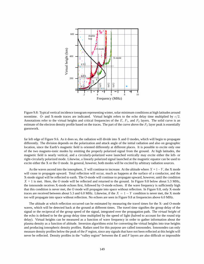
We can now begin to address the question of what happens to RF radiation launched vertically into the ionospherefrom the ground. A special kind of radar used to to probe the ionosphere by transmitting HF signals over a broadrange of frequencies and measuring the return times of the echoes is called anionosonde. The record of propagationtimes versus frequency it produces is called anionogram. An example ionogram is shown in Figure 9.8. Electrondensity profiles can be deduced, in part, from ionogram traces like those shown in the figure usually with the help ofcomputational inversion algorithms.

At ground level, there is no ionization, and the index of refraction of the wave is nearly unity. As the wave ascendsinto the ionosphere, the plasma frequency increases,X increases, and the wave effectively moves rightward from the

148

O-mode

X-mode

h’F2

h’F1

h’E

foE

foF

1

foF

2

fxF

2

doublehop

200

400

600

Virt

ual h

eigh

t (km

)

2 4 6 8 10

Frequency (MHz)

Figure 9.8: Typical vertical incidence ionogram representing winter, solar minimum conditions at high latitudes aroundnoontime. O- and X-mode traces are indicated. Virtual height refers to the echo delay time multiplied byc/2.Annotations refer to the virtual heights and critical frequencies of theE, F1, andF2 layers. The solid curve is anestimate of the electron density profile based on the traces.The part of the curve above theF2 layer peak is essentiallyguesswork.

far left edge of Figure 9.6. As it does so, the radiation will divide into X and O modes, which will begin to propagatedifferently. The division depends on the polarization and attack angle of the initial radiation and also on geographiclocation, since the Earth’s magnetic field is oriented differently at different places. It is possible to excite only oneof the two magneto-ionic modes by emitting the properly polarized signal from the ground. At high latitudes, themagnetic field is nearly vertical, and a circularly-polarized wave launched vertically may excite either the left- orright-circularly polarized mode. Likewise, a linearly polarized signal launched at the magnetic equator can be used toexcite either the X or the O mode. In general, however, both modes will be excited by arbitrary radiation sources.

As the waves ascend into the ionosphere,X will continue to increase. At the altitude whereX = 1−Y , the X modewill cease to propagate upward. Total reflection will occur,much as happens at the surface of a conductor, and theX-mode signal will be reflected to earth. The O-mode will continue to propagate upward, however, until the conditionX = 1 is met. Here, the O mode will be reflected and returned to theground. In Figure 9.8 below about 5.3 MHz,the ionosonde receives X-mode echoes first, followed by O-mode echoes. If the wave frequency is sufficiently highthat this condition is never met, the O mode will propagate into space without reflection. In Figure 9.8, only X-modetraces are received between about 5.3 and 6.0 MHz. Likewise,if theX = 1 − Y condition is never met, the X modetoo will propagate into space without reflection. No echoes are seen in Figure 9.8 at frequencies above 6.0 MHz.

The altitude at which reflection occurred can be estimated bymeasuring the travel times for the X- and O-modewaves, which will be detected back at the ground at differenttimes. The travel time signifies the group delay of thesignal or the reciprocal of the group speed of the signal, integrated over the propagation path. Thevirtual height ofthe echo is defined to be the group delay time multiplied by thespeed of light (halved to account for the round tripdelay). Virtual heights can be measured as a function of wavefrequency in order to gather information about theplasma density as a function of altitude. Inversion algorithms exist for converting the virtual heights into true heightsand producing ionospheric density profiles. Radars used forthis purpose are called ionosondes. Ionosondes can onlymeasure density profiles below the peak of theF region, since any signals that have not been reflected at thisheight willnever be reflected. Density profiles in the “valley region” between theE andF layers are also difficult or impossible

149

nz

nx

0

A B

A’ B’

1

.2.4

.6.8

X=1magneticfield

A,B A’ B’

Figure 9.9: Raytracing the O-mode wave in the plane of the magnetic meridian in the southern hemisphere. Themagnetic dip angle is set to 45. (left) Refractive index surfaces for O-mode propagation with Y < 1 (oversimplifiedsketch). The numbers indicate the value ofX for which the given surface was drawn. The radius of a point onasurface is the index of refractionn(ω, θ) calculated for the given frequency and angle. Vertical lines represent phasenormal directions for waves obeying Snell’s law. Corresponding ray normal directions are normal to the refractiveindex surfaces. (right) O-mode rays launched with different zenith angles.

to measure, being obscured byE layer ionization.

The preceding discussion is accurate for vertical incidence but is incomplete and does not address the ray pathsof the magneto-ionic modes. For that, we need to analyze the refractive index surface for the two modes. Figure 9.9(left panel) shows the O-mode refractive index surfaces. Here, the labels indicate the values ofX corresponding to thedifferent surfaces. TheX = 0 surface is a circle of radius 1. TheX = 1 surface collapses to a straight line that passesthrough the origin. Surfaces at intermediate values ofX are ellipsoids. The surfaces have been rotated 45 clockwiseso that the direction of the magnetic field is pointed up and tothe right. The figure can be viewed as describing wavepropagation looking westward in the plane of the magnetic meridian in the southern hemisphere.

The two vertical lines superimposed on the refractive indexsurfaces represent the wave normals of two waveslaunched from the ground into a vertically stratified ionosphere. Snell’s law demands that the index of refraction timesthe sine of the zenith angle of the wave normal is a constant, which is the equation for a vertical line in this figure. Thegreater the initial zenith angle of the wave, the greater thedistance of the vertical line from the origin of the figure.

As the waves propagate into and then out of the ionosphere, the ray normal directions are given by the plottedarrows, which are everywhere normal to the refractive indexsurfaces. Consider first the behavior of the waveBB′.At the ground, the plasma frequency is zero, andX = 0. As the wave enters the ionosphere,X increases, and theray normal direction rotates clockwise. Eventually, the ray normal direction turns downward, and the wave exits theionosphere. The turning point occurs in a region whereX < 1, and so the O-mode reflection height is never reached.The ray path of the wave is illustrated in the right panel of Figure 9.9.

Next, consider what happens to the rayAA′, which is launched at a much smaller zenith angle. The ray normaldirection of this wave initially rotatescounterclockwise. At the point where it intersects theX = 1 refractive indexsurface, the ray normal direction is normal to the directionof the magnetic field. At this point, which is termed the‘Spitze’, the ray direction reverses, the wave reflects, andit returns through a cusp along the same path through whichit came. The ray normal direction rotates clockwise until the wave exits the ionosphere and returns to the ground. Incases where the Spitze exists, reflection occurs at theX = 1 height. The range of initial zenith angles for which thereis a Spitze is termed the Spitze angle.

Contrast this behavior with that of the X-mode, which is depicted in Figure 9.10. For the X-mode, the refraction

150

nz

nx

0

A B

A’ B’

.1.2

X=1-Y

magneticfield

A,B A’ B’

.4

Figure 9.10: Raytracing the X-mode wave in the plane of the magnetic meridian in the southern hemisphere. (left)Refractive index surfaces for X-mode propagation withY < 1 andX < 1 (oversimplified sketch). (right) X-moderays launched with different zenith angles.

index surface collapses to a point atX = 1−Y rather than to a line; there is consequently no Spitze. Waveslaunchedwith finite zenith angles have turning points below theX = 1 − Y altitude. Waves launched with small zenith anglesare deflected so as to propagate nearly parallel to the magnetic field near the turning point. For both the X- and O-modewave solutions, rays return to the ground along the paths by which they entered if the initial incidence is vertical. Notealso that the ray paths are reversible.

The X mode is evanescent between1 − Y < X < Xuh but propagates again in the regimeXuh < X < 1 + Y ,where it is usually referred to as the Z mode. (It is possible to construct refractive index surfaces for the Z mode, justas it was for the X and O modes.) Since the X and O modes are cutoff below this range of frequencies, it is difficult tocouple radio waves launched from the ground into the Z mode. However, inspection of Figure 9.6 shows that the O andZ modes make contact atX = 1. Referring to the left panel of Figure 9.9, the point of contact corresponds to eitherend of theX = 1 line. Waves launched at zenith angles so as to intersect either endpoint can be converted from theO mode to the Z mode at the Spitze. From there, it can be shown (by examining the Z-mode refractive index surfaces– not plotted) that the radiation will propagate nearly horizontally near theX = 1 − Y 2 stratum. This radiation willnot return to the ground and appear in an ionogram unless additional reflection caused by horizontal inhomogeneityoccurs.

9.4.8 Generalized raytracing in inhomogeneous, anisotropic media

9.4.9 Attenuation and absorption

Collisions mainly between the electrons and neutral atmospheric constituents give rise to Ohmic heating, and the signalis attenuated as a result. The phenomenon is usually termed absorption in the ionosphere. In an anisotropic plasma (nobackground magnetic field), absorption is governed by (9.5), which retains the electron collision frequency. DefiningZ = ν/ω, that equation can be expressed as:

n2 = 1 −X

(

1 + jZ

1 + Z2

)

which shows how the index of refraction becomes complex. In the limit thatZ ≪ 1, which holds for most of the HFband and higher frequencies, the real part of the index of refraction is nearly unaffected by collisions. This implies thatthe ray paths are also unaffected. The imaginary part of the index of refraction, meanwhile, gives rise to attenuation

151

of the signal power, which will be governed by the factor

exp

(

−2k

∫

s

ℑ(n)ds

)

∼ exp

(

k

∫

s

XZds

)

wherek = ω/c and where the integration is over the unperturbed ray path. The factor of 2 comes from the fact that thepower is proportional to the square of the signal amplitude.In the case of radar experiments, the path should includethe incident and scattered ray paths.

Absorption occurs where the product of the plasma number density and electron collision frequency is high. Thecollision frequency decreases rapidly with height in the ionosphere, whereas the number density increases rapidlybelow theF peak. The product is greatest in the D region, which is only present at low and middle latitudes during theday. There, absorption is only important during the day and at frequencies of a few MHz or less. At high latitudes,the D region can be populated by energetic particle precipitation when and where the aurora are active. Very dense Dregion ionization associated with auroral activity can give rise to significant absorption even at VHF frequencies. Notethat when the collision frequency is sufficiently high, the cutoff even vanishes.

The isotropic limit (approximation) holds in a realistic, anisotropic ionospheric plasma so long as the wave fre-quency is much greater than the cyclotron frequency. At frequencies less than about 30 MHz, however, anisotropy canstart to have significant effects. Including the backgroundmagnetic field and retaining the electron collision frequencyin the derivation, the Appleton-Hartree equation can be shown to assume the form:

n2 = 1 − X

1 − jZ − Y 2

T

2(1−X−jZ) ±√

Y 4

T

4(1−X−jZ)2 + Y 2L

≡ (µ+ jχ)2

whereµ = nr andχ = ni are referred to as the refractive index and the absorption coefficient in this context. This isa complicated expression, best evaluated computationally. It is illustrative, however, to consider what happens in thequasi-longitudinal (θ ∼ 0) and quasi-transverse (θ ∼ π/2) limits.

The quasi-longitudinal limit applies in situations whereY 2T /2YL ≪ |(1 −X) − jZ| and as usually quoted as

n2L,R ≈ 1 − X

1 − jZ ± |YL|

Depending on the frequency, the quasi-longitudinal limit applies to angles more than a few degrees from perpendic-ular propagation. In the opposite limit, which applies onlyvery close to perpendicular, there is the quasi-transverseapproximation:

n2O ≈ 1 − X sin2 θ

1 − jZ −X cos2 θ

n2X ≈ 1 − X(1 −X − jZ)

(1 − jZ)(1 −X − jZ) − Y 2T

Absorption coefficients are calculated accordingly. The general expressions are quite complicated, but simple resultscan be obtained in various limiting situations. Information about the collision frequency profile can be derived bycomparing the measured O- and X-mode absorption.

9.4.10 Faraday rotation

Another feature of wave propagation in anisotropic media isthe progressive change of polarization along the propa-gation path. Each magneto-ionic mode has a characteristic polarization, and the polarization of two coincident modesare orthogonal. A signal with arbitrary polarization can therefore be viewed as the superposition of two orthogonal

152

magneto-ionic modes. As these two modes propagate, they obey different dispersion relations, and their phases varyspatially at different rates. The polarization of the combined wave they form is a function of their relative phases.Consequently, polarization can change along the path. One manifestation of this phenomenon is known as Faradayrotation, where the plane of a linearly polarized signal rotates in space.

Consider a linearly polarized wave propagating parallel tothe magnetic field in the high frequency limit. Thiswave is the sum of left and right circularly polarized magneto-ionic modes with equal amplitudes. At any point inspace, the electric fields of the two modes rotate with the same angular frequency in time but in opposite directions.Measured clockwise from thex axis, the angles of the electric fields of the modes areφL and−φR, which are justthe phase angles of the modes. The angle of the plane of polarization of the linearly polarized wave formed by thetwo is then the average, or(φL − φR)/2. This angle is constant at any given point in space. Since thewavelengths ofthe magneto-ionic modes are different, however, the phase differenceφL − φR will vary spatially in the direction ofpropagation, and the plane of the linearly polarized wave will rotate in space.

The fields of the left- and right-circularly polarized modesvary along the paths as

EL,R(s) ∼ exp

[

j

(

ωt− k

∫

s

n±(s)ds

)]

where the indices of refraction for parallel propagation inthe high-frequency, collisionless limit are

n± =

(

1 − X

1 ± Y

)1/2

∼ 1 − X

2(1 ∓ Y )

Consequently, the accumulated difference in the phase of the left- and right-circularly polarized waves along the pathis

∆φ = φL − φR =

∫

s

X(s)Y (s)ds

=e3

cm2eǫ

1

ω2

∫

s

N(s)B(s)ds

If the propagation is not quite parallel to the magnetic fieldbut falls within the quasi-longitudinal limit, this expressioncan be written more generally as (in SI units)

∆φ =4.73 × 104

f2

∫

s

N(s)B(s) cos θ ds

This formula shows how the plane of polarization of a linearly polarized wave∆φ/2 rotates incrementally in a plasmawith a background magnetic field. This phenomena can be used to measure the path-integrated plasma number densityor magnetic field in a space plasma presuming that the other quantity is somehow known. Differential measurementsof the Faraday angle with distance can yield entire profiles of one or the other of these quantities. Differential mea-surements can be made using spacecraft in relative motion toeach other or from radar scatter from different strata in aspace plasma. Care must be taken to sample the Faraday angle with sufficient spatial resolution to avoid problems dueto aliasing.

Faraday rotation must be taken into account when operating aradio link or radar across the ionosphere. A linkmade using only linearly-polarized antennas will suffer polarization mismatch and fading as the plane of polarizationof the received signal changes. Spacecraft communicationsare often conducted with circularly-polarized signals,which approximate a magneto-ionic mode in the quasi-longitudinal limit and so do not undergo Faraday rotation. Iflinear-polarized signals are used for transmission, both orthogonal polarizations must be received in order to recoverall of the power in the link. Circularly-polarized receive antennas will not suffer fading but will not recover all theincident power. All of these considerations cease to be important at frequencies well in excess of the plasma frequency(e.g. UHF and above) when the ionospheric plasma is well described by the isotropic approximation.

Note that reciprocity does not hold in this medium. Considera pair of transceivers using dipole antennas orientednormal to the line separating them and rotated 45 from one another. Because of Faraday rotation, it would be possiblefor a communication link so constructed to be perfectly efficient for signals going one way and perfectly inefficient

153

for signals going the other. Reciprocity is restored in a broader sense if the direction of the magnetic field is reversedwhen the roles of the transmitter and receiver are exchanged, however. Note too that, in any event, this argument doesnot alter the equivalence of antenna effective area and gain.

9.5 References

9.6 Problems

154