annual greenland accumulation rates (2009--2012) from airborne

TCD9, 6697–6731, 2015

Annual Greenlandaccumulation rates(2009–2012) from

airborne Snow Radar

L. S. Koenig et al.

Title Page

Abstract Introduction

Conclusions References

Tables Figures

J I

J I

Back Close

Full Screen / Esc

Printer-friendly Version

Interactive Discussion

Discussion

Paper

|D

iscussionP

aper|

Discussion

Paper

|D

iscussionP

aper|

The Cryosphere Discuss., 9, 6697–6731, 2015www.the-cryosphere-discuss.net/9/6697/2015/doi:10.5194/tcd-9-6697-2015© Author(s) 2015. CC Attribution 3.0 License.

This discussion paper is/has been under review for the journal The Cryosphere (TC).Please refer to the corresponding final paper in TC if available.

Annual Greenland accumulation rates(2009–2012) from airborne Snow RadarL. S. Koenig1, A. Ivanoff2, P. M. Alexander3,4, J. A. MacGregor5, X. Fettweis6,B. Panzer7, J. D. Paden7, R. R. Forster8, I. Das9, J. McConnell10, M. Tedesco4,9,C. Leuschen7, and P. Gogineni7

1National Snow and Ice Data Center, University of Colorado, Boulder, CO, USA2ADNET Systems, Inc., Bethesda, MD, USA3NASA Goddard Institute for Space Studies, New York, NY, USA4City College of New York, New York, NY, USA5Institute for Geophysics, The University of Texas at Austin, Austin, TX, USA6Department of Geography, University of Liège, Belgium7Center for Remote Sensing of Ice Sheets, University of Kansas, Lawrence, KS, USA8Department of Geography, University of Utah, Salt Lake City, UT, USA9Lamont-Doherty Earth Observatory, Columbia University, New York, NY, USA10Division of Hydrologic Science, Desert Research Institute, NV, USA

6697

http://www.the-cryosphere-discuss.net

http://www.the-cryosphere-discuss.net/9/6697/2015/tcd-9-6697-2015-print.pdf

http://www.the-cryosphere-discuss.net/9/6697/2015/tcd-9-6697-2015-discussion.html

http://creativecommons.org/licenses/by/3.0/

TCD9, 6697–6731, 2015


airborne Snow Radar

L. S. Koenig et al.

Title Page



Tables Figures

J I

J I

Back Close

Full Screen / Esc



Discussion

Paper

|D

iscussionP

aper|

Discussion

Paper

|D

iscussionP

aper|

Received: 13 November 2015 – Accepted: 24 November 2015 – Published:10 December 2015

Correspondence to: L. S. Koenig ([email protected])

Published by Copernicus Publications on behalf of the European Geosciences Union.

6698





TCD9, 6697–6731, 2015


airborne Snow Radar

L. S. Koenig et al.

Title Page



Tables Figures

J I

J I

Back Close

Full Screen / Esc



Discussion

Paper

|D

iscussionP

aper|

Discussion

Paper

|D

iscussionP

aper|

Abstract

Contemporary climate warming over the Arctic is accelerating mass loss from theGreenland Ice Sheet (GrIS) through increasing surface melt, emphasizing the needto closely monitor surface mass balance (SMB) in order to improve sea-level rise pre-dictions. Here, we quantify accumulation rates, the largest component of GrIS SMB,5

at a higher spatial resolution than currently available, using Snow Radar stratigraphy.We use a semi-automated method to derive annual-net accumulation rates from air-borne Snow Radar data collected by NASA’s Operation IceBridge from 2009 to 2012.An initial comparison of the accumulation rates from the Snow Radar and the outputsof a regional climate model (MAR) shows that, in general, the radar-derived accumu-10

lation matches closely with MAR in the interior of the ice sheet but MAR estimates arehigh over the southeast GrIS. Comparing the radar-derived accumulation with contem-poraneous ice cores reveals that the radar captures the annual and long-term mean.The radar-derived accumulation rates resolve large-scale patterns across the GrIS withuncertainties of up to 11 %, attributed mostly to uncertainty in the snow/firn density pro-15

file.

1 Introduction

Contemporary climate warming over the Greenland Ice Sheet (GrIS) has acceler-ated its mass loss, nearly quadrupling from ∼ 55 Gtyr−1 between 1993–99 (Krabillet al., 2004) to ∼ 210 Gtyr−1 of ice, equivalent to ∼ 0.6 mmyr−1 of sea level rise, be-20

tween 2003–08 (Shepherd et al., 2012). As GrIS mass loss has accelerated, a funda-mental change in the nature of this loss has occurred. The dominant mass loss processfor the GrIS is changing from being governed by ice dynamics to being dominated bysurface mass balance (SMB) processes (van den Broeke, 2009; Enderlin et al., 2014).This recent shift emphasizes the need to monitor SMB which, over most of the GrIS, is25

dominated by net accumulation.

6699





TCD9, 6697–6731, 2015


airborne Snow Radar

L. S. Koenig et al.

Title Page



Tables Figures

J I

J I

Back Close

Full Screen / Esc



Discussion

Paper

|D

iscussionP

aper|

Discussion

Paper

|D

iscussionP

aper|

Here we use the complete set of airborne Snow Radar data collected by NASA’sOperation IceBridge (OIB) over the GrIS from 2009 to 2012 to produce annual-netaccumulation rates, here after called accumulation for simplicity, along those flightlines.The radar-derived accumulation rates are compared to both in situ data and modeloutputs from the Modèle Atmosphérique Régional (MAR).5

2 Background

In situ accumulation-rate measurements are limited by the time and cost of acquiringice cores, digging snow pits or monitoring stake measurements across large sectors ofthe ice sheet. Only two major accumulation-rate measurement campaigns have beenundertaken across the GrIS, the first in the 1950’s when the US Army collected pit data10

along long traverse routes (Benson, 1962) and the second in the 1990’s when the Pro-gram on Arctic and Regional Climate Assessment (PARCA) collected an extensivelydistributed set of ice cores (e.g. Mosley-Thompson et al., 2001). A recent traverse andstudy by Hawley et al. (2014) reports a 10 % increase in accumulation since the 1950’sand highlights the need to monitor how Greenland precipitation is evolving in the midst15

of ongoing climate change. Although many other accumulation-rate measurements ex-ist, they are more limited in either space or time (e.g. Dibb and Fahnestock, 2004;Hawley et al., 2014).

To date there is no annually resolved satellite-retrieval algorithm for accumulationrate across ice sheets. Hence, the two primary methods used to generate large-scale20

(hundreds of km) accumulation-rate patterns are model predictions and radar-derivedaccumulation rates (Koenig et al., 2015). High resolution, near-surface radar data haveshown good fidelity at mapping spatial patterns of accumulation over ice sheets atdecadal and annual resolutions from both airborne and ground-based radars (Kana-garatnam et al., 2001, 2004; Spikes et al., 2004; Arcone et al., 2005; Anshütz et al.,25

2008; Müller et al., 2010; Medley et al., 2013; Hawley et al., 2006, 2014; de la Peña et al., 2010; Miège et al., 2013). Radars detect and map isochronal layers within the

6700





TCD9, 6697–6731, 2015


airborne Snow Radar

L. S. Koenig et al.

Title Page



Tables Figures

J I

J I

Back Close

Full Screen / Esc



Discussion

Paper

|D

iscussionP

aper|

Discussion

Paper

|D

iscussionP

aper|

firn. When these layers are either (1) dated in conjunction with ice cores or (2) annuallyresolved from the surface, they can be used to determine along-track accumulationrates.

Early studies by Spikes et al. (2004) in Antarctica and Kanagaratnam et al. (2001 and2004) in Greenland used high/very high-frequency (100 to 1000 MHz) ground-based5

and airborne radars, with vertical resolutions of ∼ 30 cm, to monitor decadal-scale ac-cumulation rates between dated ice cores. These high/very high-frequency radars canpenetrate to hundreds of meters in the dry-snow zone and tens of meters in the ab-lation zone (Kanagaratnam et al., 2004). Subsequent studies utilized the larger band-widths of ultra/super-high frequency (2 to 20 GHz), frequency-modulated continuous10

wave (FMCW) radars, with centimeter-scale vertical resolutions capable of mappingannual layers within ice sheets (e.g. Legarsky, 1999; Marshall and Koh, 2008; Medleyet al., 2013). Ultra/super-high frequency radars can penetrate tens of meters in thedry-snow zone and meters in the ablation zone. Legarsky (1999) was among the firstto show that such radars could image annual layers, and Hawley et al. (2006) further15

demonstrated that a 13.2 GHz (Ku-band) airborne radar imaged annual layers in thedry-snow zone of the GrIS to depths of up to 12 m.

Most previous studies used radar data that overlapped spatially with ice cores orsnow pits for both dating layers and density information. Medley et al. (2013) and Daset al. (2015), however, showed that accumulation rates could be derived using density20

from a regional ice core ensemble. The end members of density are used as the un-certainty limits and the derived regional density profile is sufficient for radar studies ofaccumulation and SMB (Das et al., 2015). Additionally, Medley et al. (2013) showedthat the Snow Radar was capable of resolving annual layering in high accumulationregions where the layers were preserved and, therefore, it was possible to date the25

layers by counting from the surface downwards.Regional and Global Climate Models (RCMs and GCMs) and reanalysis products

provide the only spatially and temporally extensive estimates of accumulation-ratefields at ice-sheet scales (e.g. Burgess et al., 2010; Hanna et al., 2011; Ettema et al.,

6701





TCD9, 6697–6731, 2015


airborne Snow Radar

L. S. Koenig et al.

Title Page



Tables Figures

J I

J I

Back Close

Full Screen / Esc



Discussion

Paper

|D

iscussionP

aper|

Discussion

Paper

|D

iscussionP

aper|

2009; Fettweis, 2007; Cullather et al., 2014). In a comprehensive model intercompar-ison study, Vernon et al. (2013) found that modelled accumulation rates had the leastspread across RCM’s but still had a ∼ 20 % variance. Chen et al. (2011) found the rangein average accumulation across the GrIS between 5 reanalysis models to be ∼ 15 to30 cmyr−1, while Cullather and Bosilovich (2011) found the range in average accumu-5

lation across the GrIS between reanalysis data and RCM’s to be ∼ 34 to 42 cmyr−1.Overall, while these models continue to improve, there is clearly a continuing need forlarge-scale accumulation-rate measurements to evaluate their outputs.

3 Data, instruments and model description

3.1 Snow radar and data10

Annual layers in the GrIS snow/firn were mapped using the University of Kansas’Center for Remote Sensing of Ice Sheets (CReSIS) ultra-wideband Snow Radarduring NASA’s Operation IceBridge (OIB) Arctic Campaigns from 2009 through2012 (Leuschen, 2014). The radar operates over the frequency range from ∼ 2 to6.5 GHz (Panzer et al., 2013; Rodriguez-Morales et al., 2014). The Snow Radar uses15

a Frequency-Modulated Continuous Wave (FMCW) design to provide a vertical-rangeresolution of ∼ 4 cm in snow/firn, capable of resolving annual layering, when preserved,to tens of meters in depth (Medley et al., 2013).

3.2 Modelled accumulation rates and density

Accumulation rate and snow/firn density profiles were derived from the MAR RCM20

(v3.5.2; X. Fettweis, personal communication, 2015). MAR is a coupled surface–atmosphere model that simulates fluxes of mass and energy in the atmosphere and be-tween the atmosphere and the surface in three dimensions, and is forced at the lateralboundaries with climate reanalysis outputs (Gallée, 1997; Gallée and Schayes, 1994;Lefebre et al., 2003). It incorporates the atmospheric model of Gallée and Schayes25

6702





TCD9, 6697–6731, 2015


airborne Snow Radar

L. S. Koenig et al.

Title Page



Tables Figures

J I

J I

Back Close

Full Screen / Esc



Discussion

Paper

|D

iscussionP

aper|

Discussion

Paper

|D

iscussionP

aper|

(1994), and the Soil Ice Snow Vegetation Atmosphere Transfer scheme (SISVAT) landsurface model, which includes the multi-layer Crocus snow model of Brun et al. (1992).The MAR v3.5.2 simulation used here utilizes reanalysis outputs from the EuropeanCenter for Medium Range Weather Forecasting (ECMWF) ERA-Interim (Dee et al.,2011) at the lateral boundaries, with a horizontal resolution of 25 km. The details of5

this setup are described further by Fettweis (2007), with further updates described byFettweis et al. (2011, 2013) and Alexander et al. (2014). MAR has been validated within situ data and remote sensing data over GrIS, including data from weather stations(e.g. Lefebre et al., 2003; Fettweis et al., 2011), in situ and remote sensing albedodata (Alexander et al., 2014), and ice-core accumulation-rate estimates (Colgan et al.,10

2015), and it has been used to model both past and future SMB (Fettweis et al., 2005,2013). We use accumulation-rate and density profiles simulated by MAR for the periodduring which the radar data were collected (2009 to 2012).

3.3 In situ density and accumulation data

The SUrface Mass balance and snow depth on sea ice working group (SUMup) dataset15

(July 2015 release) contains a compilation of publically available accumulation, snowdepth and density measurements over both sea ice and ice sheets (Koenig et al.,2012). We use two subsets of this data. First, to characterize density across the GrIS,we extract the snow/firn density measurements ranging in depth from the snow surfaceto 15 m (the depth to which MAR predicts firn densities), which contains over 150020

measurements from snow pits and ice cores (Koenig et al., 2015, 2014; Miège et al.,2013; Mosley-Thompson et al., 2001; Hawley et al., 2014; Baker, 2015) (Fig. 1). Sec-ond, to compare radar-derived and measured accumulation rates, we consider onlyaccumulation-rate measurements within 5 km of OIB Snow Radar data, a criterion thatincludes 11 ice cores from the SUMup dataset (Mosley-Thompson et al., 2001). To25

expand this comparison, an additionally dataset of 71 ice cores (J. McConnell, per-sonal communication, 2015) which includes additional cores to the SUMup dataset,

6703





TCD9, 6697–6731, 2015


airborne Snow Radar

L. S. Koenig et al.

Title Page



Tables Figures

J I

J I

Back Close

Full Screen / Esc



Discussion

Paper

|D

iscussionP

aper|

Discussion

Paper

|D

iscussionP

aper|

was used to locate accumulation measurements within 5 km of OIB Snow Radar dataproviding 23 additional ice cores (Fig. 1).

4 Methods

4.1 Determining the density profile and uncertainties

Because we seek to derive accumulation rates from near-surface radars across large5

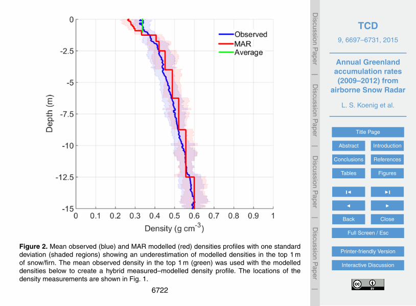
portions of the ice sheet, we require firn density profiles that cover and vary acrossthe GrIS. Modelled snow/firn density profiles from the MAR model were investigatedfor use. However, a preliminary comparison of the SUMup-measured density pro-files to MAR-estimated density profiles showed that MAR simulated density values inthe top 1 m of snow/firn were significantly lower (0.284±0.050 gcm−3) than observed10

(0.338±0.039 gcm−3) (Fig. 2). We consider it beyond the scope of this study to inves-tigate and explain why MAR underestimates near-surface density, therefore, here weassume that the firn density in the top 1 m is 0.338 gcm−3. Below 1 m, the model andobserved densities are similar (4 % mean difference), so the spatially-varying modelleddensity profiles are used. Hence, a hybrid measured-modelled density profile is used15

to determine accumulation rates from the snow radar data (Fig. 2).Uncertainty in the top meter is assigned by the ±1σ variation in observed density

(12 %). We note that this uncertainty is broadly consistent with that which we expectdue to natural variability in surface density across the GrIS. This natural variation, how-ever, represents a smaller assumed error than the mean difference between the mod-20

elled and observed values within the top 1 m (16 %).

4.2 Deriving accumulation rates from Snow Radar and uncertainties

The radar travel time is converted to depth (z) using the snow/firn density profile andthe dielectric mixing model of Looyenga (1965). Possible errors in radar-derived depth

6704





TCD9, 6697–6731, 2015


airborne Snow Radar

L. S. Koenig et al.

Title Page



Tables Figures

J I

J I

Back Close

Full Screen / Esc



Discussion

Paper

|D

iscussionP

aper|

Discussion

Paper

|D

iscussionP

aper|

come from two sources: (1) the dielectric mixing model chosen and (2) layer pick-ing. The choice of the dielectric mixing model maximizes potential error at a densityof ∼ 0.300 gcm−3. The maximum possible difference in depth over 15 m is 3 % as-suming a constant density of 0.320 gcm−3 and < 1 % assuming a constant density of0.600 gcm−3 (Wiesmann and Matzler, 1999; Gubler and Hiller, 1984; Schneebeli et al.,5

1998; Looyenga, 1965; Tiuri et al., 1984). The second source of error occurs duringmanual adjustment of the picked layers (Sect. 4.3.4) and is estimated to be ±3 bins or∼ 8 cm.

Accumulation rate is derived using the standard equation for converting depth froma radar profile to accumulation rates at location (x):10

b(x) =TWT(x)ρ(x)c

2a(x)ρw

(ρ(x)ρi

(ε′1/3i −1

)+1

)3/2(1)

Where b is water equivalent accumulation rate in mw.e.yr−1, TWT is the two-way traveltime to the dated layer in sec, ρ is cumulated snow/firn density at that depth in kgm−3,c is the speed of light in ms−3, a is age of the layer in years from the date of radardata collection, ρw is water density in kgm−3, ρi is ice density in kgm−3 and ε′i is the15

dielectric permittivity of ice. The cumulative snow/firn density (ρ) is determined by thedensity profile previously described in Sect. 4.1. The layers are picked in the radar datausing a semi-automated approach (Sect. 4.3).

Layer ages are determined by assuming spatially continuous layers are annuallyresolved and dated accordingly from the year the radar data were collected. The radar20

data were collected during springtime (April–May) and the surface is assumed to be 30April. The picked layers at depth are assumed to be 1 July ±1 month as follows. A peakin radar reflection, assuming ice with no impurities, is caused by the largest changein snow density. In the ablation and percolation zone, the peak in density differenceoccurs in the summer between the snow layer and ice or the snow/firn layer and the25

high-density melt/crust layer, respectively (e.g. Nghiem et al., 2005). In the dry snow6705





TCD9, 6697–6731, 2015


airborne Snow Radar

L. S. Koenig et al.

Title Page



Tables Figures

J I

J I

Back Close

Full Screen / Esc



Discussion

Paper

|D

iscussionP

aper|

Discussion

Paper

|D

iscussionP

aper|

zone, the peak in density difference also occurs in the summer between the summerhoar layer and the denser snow/firn layer (e.g. Alley et al., 1990).

To calculate the total uncertainty on the radar-derived accumulation rate, the max-imum error is assumed for both density (12 %) and age (8 %). Equation (1) is writtento show the relationship between the density profile, which is used both for calculating5

depth and water equivalent. The derivative of Eq. (1) is used to determine the corre-lated error between depth and density. Assuming uncorrelated and normally distributederrors between density and age, the maximum accumulation-rate uncertainty is 11 %,with uncertainty in the density profile in the top meter of firn being the largest contrib-utor. Uncertainty from our study is very similar to studies by Medley et al. (2013) and10

Das et al. (2015) for radar-derived accumulation rates.

4.3 Semi-automated radar layer picker

A semi-automated layer detection algorithm was developed to process the largeamounts of radar data gathered by OIB (> 104 kmyr−1), analogous to the challengesfaced by MacGregor et al. (2015) for analysis of very high frequency “deep” radar data.15

A previously developed semi-automated method designed by Onana et al. (2014) wastested for this application but proved too computationally intensive, with higher errorrates than the method described here. While a fully automated method is ultimatelydesirable, we have found that it is necessary to manually check every automated pick,making adjustments as needed by an experienced analyst, to distinguish between spa-20

tially discontinuous radar reflectors, caused by the normal heterogeneity of firn mi-crostructure, and spatially consistent annual layers. The algorithm processes the OIBSnow Radar data in four steps outlined below.

4.3.1 Surface alignment

The snow surface is detected by a threshold, set to four times the mean radar return25

from air, which is assumed to be the radar noise level. A median filter is applied ver-

6706





TCD9, 6697–6731, 2015


airborne Snow Radar

L. S. Koenig et al.

Title Page



Tables Figures

J I

J I

Back Close

Full Screen / Esc



Discussion

Paper

|D

iscussionP

aper|

Discussion

Paper

|D

iscussionP

aper|

tically to each radar trace to minimize data noise. In addition, any surface value thatexceeds a distance threshold of 10 range bins (∼ 25 cm) from its neighbors is not usedand that entire vertical trace is ignored in subsequent analysis. Data arrays are thenaligned to the surface and truncated above and below the surface (200 and 800 rangebins, respectively), equivalent to ∼ 25 m into the snow/firn, to reduce data volumes.5

Layer depths are measured relative to the snow surface. The radar data are then hor-izontally averaged (stacked) to an along-track spacing of ∼ 50 m, in 2011 and 2012,and ∼ 10 m, in 2009 and 2010, and split into equally sized sections of 2000 traces perradargram for easier processing.

4.3.2 Layer detection10

The algorithm takes advantage of the difference between high-frequency and low-frequency spatial variability to identify peaks in returned power in the radar data. Peaksare formed by the stratified accumulation layers, resulting in density changes, which ex-tend across the GrIS. The point at which the peak forms occurs over a small spatialscale, or at a high frequency. The peak detection process is thus a type of high-pass15

filter, resulting in the set of disjointed points in adjacent traces along the flight path.These points are stored as layer segments using the half maximum width of the peak’swaveform, resulting in continuous layer segments over the radar data profile (Fig. 3).

4.3.3 Layer indexing

Each detected layer is indexed, with both a number and the corresponding year (Fig. 3).20

This process is accomplished by indexing the layers downward from the surface. Theindexing process begins with the segmentation of the layers, so that each layer isuniquely identifiable. The peak points within each segment are then connected bysmoothed spline fits, resulting in a set of sharply defined layers. Layer indices are as-signed from top to bottom to take into account the partial overlap that can exist between25

layers.

6707





TCD9, 6697–6731, 2015


airborne Snow Radar

L. S. Koenig et al.

Title Page



Tables Figures

J I

J I

Back Close

Full Screen / Esc



Discussion

Paper

|D

iscussionP

aper|

Discussion

Paper

|D

iscussionP

aper|

4.3.4 Manual adjustment with the Layer Editor

A graphical user interface (GUI) was developed to verify the automated layer detec-tions. An analyst used the GUI to quickly compare the picked layers and the radargram.The GUI application allows for editing of the output layers as needed.

5 Results5

5.1 Radar-derived accumulation rates over the GrIS

Annual radar-derived accumulation rates and their uncertainties were calculated forall 2009–2012 OIB radar data that contained detected layers (Fig. 4). The increasein coverage from 2009 to 2012 is related to an increasing number of OIB flights overthe GrIS and adjustments to the Snow Radar antenna and operations that improved10

overall data quality. These accumulation-rate patterns are consistent with observedand modelled large-scale spatial patterns for the GrIS: high accumulation rates in thesoutheast-coastal sector and lower accumulation rates in the northeast (Fig. 5). Year-to-year variability in accumulation rate is also evident and can be seen even at theice-sheet scale, e.g., in the southeast accumulation rates were lower in 2010 than in15

2011.The radar-derived accumulation in Fig. 4 represents only the first layer detected by

the Snow Radar, or approximately the annual accumulation rate from the year priorto data collection. For simplicity, we refer to this quantity as the annual accumulationrate, but we caution that it does not strictly represent the calendar year. The values20

shown in Fig. 4 represent only 10 months of accumulation, based on our assumptionthat the radar layers date to 1 July (Sect. 4.2) and that the data collection date is 30April for all OIB data. When comparing the first layer of radar-derived accumulationto modelled estimates from MAR (Fig. 5) or other accumulation measurements, this

6708





TCD9, 6697–6731, 2015


airborne Snow Radar

L. S. Koenig et al.

Title Page



Tables Figures

J I

J I

Back Close

Full Screen / Esc



Discussion

Paper

|D

iscussionP

aper|

Discussion

Paper

|D

iscussionP

aper|

timing difference must be considered. Although the first layer represents only a partialyear, all deeper layers represent a full year, from 1 July to 30 June.

Figure 6 shows the number of detected layers, or previous years, discernable in theOIB radar data. For the majority of the GrIS, 1 to 3 annual layers are discernable,due to the spatial distribution of OIB flightlines. OIB flightlines are clustered in the5

ablation/percolation zones of the GrIS, where radar penetration depths are reduced bythe increased density, englacial water and layering structure of the firn column (Fig. 3).In the GrIS interior, where dry snow conditions allow deeper radar penetration, annuallayering going back over two decades is detectable (Fig. 3).

Crossover points were assessed to determine the internal consistency of the radar-10

derived accumulation rates (Figs. 7 and 8). While no consistent spatial pattern is foundin the crossover errors, the largest discrepancies were found in 2011 and 2012 in thenorthwest and southeast (Fig. 7). Other inconsistencies are likely due to snow stormsoccurring between flights in the southeast and incorrectly picked layers that were ei-ther sub- or multi-annual in the northwest. Figure 8 shows a scatterplot of crossover15

points. There are relatively few outliers, and those that are outlying are generally offsetby a factor of two, suggesting an error in layer detection/dating rather than a radar-system error. Crossover differences per year, including the mean, standard deviationand maximum, are listed in Table 1. Crossover differences are comparable (mean of0.04 mw.e.) to our inferred relative uncertainty of 11 % which emphasizes the overall20

validity of our chosen methods.

5.2 Comparison with modelled accumulation

The radar-derived accumulation rate was gridded to the MAR grid for comparison.The mean-local, radar-derived accumulation rate was used when gridding. BecauseOIB flightlines are not spatially heterogeneous, each MAR grid cell represents a dif-25

ferent number of radar-derived values, so grid cells are not sampled equally. With thisdiscrepancy noted, this gridding method is still the most straightforward and useful ap-proach for this comparison. Figure 9 shows the difference between the radar-derived

6709





TCD9, 6697–6731, 2015


airborne Snow Radar

L. S. Koenig et al.

Title Page



Tables Figures

J I

J I

Back Close

Full Screen / Esc



Discussion

Paper

|D

iscussionP

aper|

Discussion

Paper

|D

iscussionP

aper|

and MAR accumulation rates. The mean difference for all years is low (0.02 mw.e.).Table 1 shows the annual variability of the mean difference, which is low for every yearexcept 2010, when large differences are seen over the southeast coastal region of theGrIS (Fig. 9).

Figure 9 shows that MAR generally predicts accumulation well in the GrIS interior5

(consistent with the comparison with ice core estimates presented by Colgan et al.,2015), but has larger errors around the periphery, especially in the southeast andnorthwest. In the southeast, MAR generally overestimates accumulation rates, exceptin 2011 when there is a mixed pattern of agreement and overestimation. This pattern ofoverestimation in the southeast is not surprising and is likely due to the lack of previous10

measurements in the region to constrain accumulation and the large changes in sur-face topography that are not resolved by the relatively large grid size used in modelledestimates (Burgess et al., 2010). In 2011, the northwest coastal region of the GrIS waswell sampled by OIB and MAR shows an underestimation of accumulation rate, but theorigin of this anomaly is less clear.15

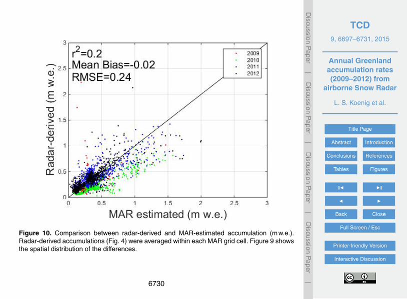
Figure 10 shows a scatterplot of the radar-derived and MAR-estimated accumu-lation rates. These values are not well correlated (Pearson correlation coefficientr2 = 0.2) and have large RMSE (0.24 mw.e.), emphasizing that further improvements inaccumulation-rate modeling are needed, particularly over the southeast and northwestGrIS.20

5.3 Comparison with annually resolved in situ data

Between 2009 and 2012, OIB flew within 5 km of 34 ice-core locations but only twolocations, NEEM and Camp Century (Fig. 1) were coincident in time with the layerswe detected. Each of these locations has two cores, providing annual accumulationrates and a measure of spatial variability. Figure 11 compares the radar-derived to25

ice-core measured accumulation rates. At NEEM, the two ice cores and radar dataare closely located, within 0.6 km of each other. The radar-derived accumulation ratesare self-consistent between 2011 and 2012 and agree well with the ice cores (Root

6710





TCD9, 6697–6731, 2015


airborne Snow Radar

L. S. Koenig et al.

Title Page



Tables Figures

J I

J I

Back Close

Full Screen / Esc



Discussion

Paper

|D

iscussionP

aper|

Discussion

Paper

|D

iscussionP

aper|

Mean Square Error (RMSE) of 0.06 mw.e.). For comparison, the two NEEM ice coreshave a RMSE of 0.05 mw.e. for the period of overlap. A timing discrepancy ariseswith this comparison because the ice cores, with higher dating resolution from isotopicand chemical analysis, are dated and reported as the calendar year, whereas as theradar-derived accumulation is assumed 30 June–1 July (Sect. 4.2). This mismatch in5

the measurement is likely evident in Fig. 11 by the differences in the annual peaksbetween the cores and radar-derived accumulation having similar means yet differingmagnitudes from year to year.

Near Camp Century, the ice cores and radar data are farther apart from each other.The radar-data are located within 4.4 km of the Camp Century core and the GITS core10

is located ∼ 8.2 km from the Camp Century core. These separations are likely respon-sible for the poorer agreement at this site of radar-derived accumulation rate to theCamp Century core (RMSE 0.10 mw.e.) and the larger difference (RMSE 0.07 mw.e.)in accumulation rate between the two cores for the period of overlap. While it is moredifficult to analyze the results at Camp Century, with only 3 points of overlap and no15

time series of radar-derived accumulation, it is evident that the radar-derived accumu-lation rates are within the expected variability and capture the long-term mean value.

6 Discussion

This study is the first to derive annual accumulation rates from near-surface airborneradar data collected across the large portions of the GrIS. The pattern of radar-derived20

accumulation rates compares well with known large-scale patterns and clearly showsthat these accumulation-rate measurements are useful for evaluating model estimates.At the two locations with contemporaneous cores, the radar-derived rates agree wellwith the long-term mean. Additional cores, with direct overflights, are clearly neededto continue assessing the accuracy of the radar-derived accumulation rates from the25

layers within the firn over the GrIS.

6711





TCD9, 6697–6731, 2015


airborne Snow Radar

L. S. Koenig et al.

Title Page



Tables Figures

J I

J I

Back Close

Full Screen / Esc



Discussion

Paper

|D

iscussionP

aper|

Discussion

Paper

|D

iscussionP

aper|

The work shown here only incorporates layering detected in the radar data that isannual and continuous from the surface to depth. It does not exhaust all layering de-tected by the Snow Radar, i.e., there are still contiguous layers in the dataset that werenot utilized. For example, in the central-northern GrIS, there is a strongly reflectinglayer varying between 15 and 18 m that cannot be dated with the radar data alone. If5

ice cores were drilled to identify this layer, techniques similar to those developed byMacGregor et al. (2015) or Das et al. (2015) could be used to determine multi-annualaccumulation rates in additional regions of the GrIS. Additionally, further deconvolutionprocessing of the radar data, currently ongoing at CReSIS, resolves additional deeplayers in the Snow Radar data that will expand accumulation measurements in the10

future.Annual-radar-derived accumulation rates are not extrapolated spatially here. Spatial

extrapolation between the constantly varying flightlines will be left for future work, asadditional data are collected and made available to fill in gaps.

Finally, the largest uncertainty in the radar-derived accumulation rate comes from15

the hybrid measured-modelled density profiles used. Spatially distributed density mea-surements and improved density models spanning the entire firn column are requiredto take full advantage of the layering detected by near-surface radars and to reducethe errors in radar-derived accumulation rates. More specifically, as shown in Fig. 1,the current sampling of measurements has large spatial gaps over the southwest-20

ern and northeastern GrIS and the majority of the measurements are located in theupper-percolation and dry-snow zones. To further constrain and improve density mod-els required for radar-derived accumulation rates, these spatial gaps and samplingdistributions need to be filled to broaden with additional measurements.

7 Conclusions25

A semi-automated method was developed to process tens of thousands of kilometersof airborne Snow Radar data collected by OIB across the GrIS between 2009 and

6712





TCD9, 6697–6731, 2015


airborne Snow Radar

L. S. Koenig et al.

Title Page



Tables Figures

J I

J I

Back Close

Full Screen / Esc



Discussion

Paper

|D

iscussionP

aper|

Discussion

Paper

|D

iscussionP

aper|

2012. The resulting radar-derived accumulation dataset represents the largest valida-tion dataset for recent annual accumulation across the GrIS to date. This dataset cap-tures the large-scale accumulation-rate patterns of the GrIS well. Over two decades ofannual radiostratigraphy is observed in the dry snow zone, near Summit Station, and1 to 3 years are generally detectable in the ablation/percolation zones. Our estimated5

uncertainty in the radar-derived accumulation is 11 %, with the largest error contribu-tion coming from the hybrid measured-modelled density profiles. This study empha-sizes the need for ice cores coincident in time with airborne overflights and, more im-portantly, for improved density profiles, particularly in the top 1 m of snow/firn. Theseradar-derived accumulation-rate datasets should be used to evaluate RCM/GCM and10

reanalysis products, as demonstrated here using the MAR model. MAR reproducesthe radar-derived accumulation rates for most of the interior of the GrIS, but tends tooverestimate accumulation rates in the southeastern coastal region of the GrIS and, inat least one year, underestimates accumulation rates in the northwestern costal regionof the GrIS. While determining the precise nature of these differences is left for future15

work, we have clearly demonstrated the usefulness of the ice-sheet-wide, radar-derivedaccumulation-rate datasets for improving SMB estimates. As the GrIS continues to losemass through SMB processes, monitoring accumulation rates directly is vital.

Acknowledgements. This work was supported by the NASA Cryospheric Sciences Programand by the NSF grant #1 304 700 and the NASA grants #NNX15AL45G and #NNX14AD98G.20

Data collection and instrument development were made possible by The University of Kansas’Center for Remote Sensing of Ice Sheets (CReSIS) supported by the National Science Foun-dation and NASA’s Operation IceBridge.

References

Alexander, P. M., Tedesco, M., Fettweis, X., van de Wal, R. S. W., Smeets, C. J. P. P.,25

and van den Broeke, M. R.: Assessing spatio-temporal variability and trends in modelledand measured Greenland Ice Sheet albedo (2000–2013), The Cryosphere, 8, 2293–2312,doi:10.5194/tc-8-2293-2014, 2014.

6713





http://dx.doi.org/10.5194/tc-8-2293-2014

TCD9, 6697–6731, 2015


airborne Snow Radar

L. S. Koenig et al.

Title Page



Tables Figures

J I

J I

Back Close

Full Screen / Esc



Discussion

Paper

|D

iscussionP

aper|

Discussion

Paper

|D

iscussionP

aper|

Alley, R. B., Saltzman, E. S., Cuffey, K. M., and Fitzpatrick, J. J.: Summertime for-mation of Depth Hoar in central Greenland, Geophys. Res. Lett., 17, 2393–2396,doi:10.1029/GL017i013p02393, 1990.

Anschütz, H., Steinhage, D., Eisen, O., Oerter, H., Horwath, M., and Ruth, U.: Small-scalespatio-temporal characteristics of accumulation rates in western Dronning Maud Land,5

Antarctica, J. Glaciol., 54, 315–323, doi:10.3189/002214308784886243, 2008.Arcone, S. A., Spikes, V. B., and Hamilton, G. S.: Phase structure of radar stratigraphic horizons

within Antarctic firn, Ann. Glaciol., 41, 10–16, doi:10.3189/172756405781813267, 2005.Benson, C. S.: Stratigraphic studies in the snow and firn of the Greenland Ice sheet, SIPRE

Res. Rep., 70, 1–89, 1962.10

Baker, I.: Density and permeability measurements with depth for the NEEM 2009S2firn core, ACADIS Gateway, https://www.aoncadis.org/dataset/neem_firn_core_2009s2_density_and_permeability.html, 2015.

Brun, E., David, P., Sudul, M., and Brunot, G.: A numerical model to simulate snow-cover stratig-raphy for operational avalanche forecasting, J. Glaciol., 38, 13–22, 1992.15

Burgess, E. W., Forster, R. R., Box, J. E., Mosley-Thompson, E., Bromwich, D. H., Bales, R. C.,and Smith, L. C.: A spatially calibrated model of annual accumulation rate on the GreenlandIce Sheet (1958–2007), J. Geophys. Res., 115, F02004, doi:10.1029/2009JF001293, 2010.

Chen, L., Johannessen, O. M., Wang, H., and Ohmura, A.: Accumulation over the Green-land Ice Sheet as represented in reanalysis data, Adv. Atmos. Sci., 28, 1030–1038,20

doi:10.1007/s00376-010-0150-9, 2011.Colgan, W., Box, J. E., Andersen, M. L., Fettweis, X., Csathó, B., Fausto, R. S., Van As, D., and

Wahr, J.: Greenland high-elevation mass balance: inference and implication of reference pe-riod (1961–90) imbalance, Ann. Glaciol., 56, 105–117, doi:10.3189/2015AoG70A967, 2015.

Cullather, R. I. and Bosilovich, M. G.: The Energy Budget of the Polar Atmosphere in MERRA,25

J. Climate, 25, 5–24, doi:10.1175/2011JCLI4138.1, 2012.Cullather, R. I., Nowicki, S. M., Zhao, B., and Suarez, M. J.: Evaluation of the surface represen-

tation of the Greenland Ice Sheet in a general circulation model, J. Climate, 27, 4835–4856,2014.

Das, I., Scambos, T. A., Koenig, L. S., van den Broeke, M. R., and Lenaerts, J. T. M.: Extreme30

wind-ice interaction over Recovery Ice Stream, East Antarctica, Geophys. Res. Lett., 42,2015GL065544, doi:10.1002/2015GL065544, 2015.

6714





http://dx.doi.org/10.1029/GL017i013p02393

http://dx.doi.org/10.3189/002214308784886243

http://dx.doi.org/10.3189/172756405781813267

https://www.aoncadis.org/dataset/neem_firn_core_2009s2_density_and_permeability.html



http://dx.doi.org/10.1029/2009JF001293

http://dx.doi.org/10.1007/s00376-010-0150-9

http://dx.doi.org/10.3189/2015AoG70A967

http://dx.doi.org/10.1175/2011JCLI4138.1

http://dx.doi.org/10.1002/2015GL065544

TCD9, 6697–6731, 2015


airborne Snow Radar

L. S. Koenig et al.

Title Page



Tables Figures

J I

J I

Back Close

Full Screen / Esc



Discussion

Paper

|D

iscussionP

aper|

Discussion

Paper

|D

iscussionP

aper|

Dee, D. P., Uppala, S. M., Simmons, A. J., Berrisford, P., Poli, P., Kobayashi, S., Andrae, U.,Balmaseda, M. A., Balsamo, G., Bauer, P., Bechtold, P., Beljaars, A. C. M., van de Berg, L.,Bidlot, J., Bormann, N., Delsol, C., Dragani, R., Fuentes, M., Geer, A. J., Haimberger, L.,Healy, S. B., Hersbach, H., Hólm, E. V., Isaksen, L., Kållberg, P., Köhler, M., Matricardi, M.,McNally, A. P., Monge-Sanz, B. M., Morcrette, J.-J., Park, B.-K., Peubey, C., de Rosnay, P.,5

Tavolato, C., Thépaut, J.-N., and Vitart, F.: The ERA-Interim reanalysis: configuration andperformance of the data assimilation system, Q. J. Roy. Meteor. Soc., 137, 553–597,doi:10.1002/qj.828, 2011.

de la Peña, S., Nienow, P., Shepherd, A., Helm, V., Mair, D., Hanna, E., Huybrechts, P., Guo, Q.,Cullen, R., and Wingham, D.: Spatially extensive estimates of annual accumulation in the dry10

snow zone of the Greenland Ice Sheet determined from radar altimetry, The Cryosphere, 4,467–474, doi:10.5194/tc-4-467-2010, 2010.

Dibb, J. E. and Fahnestock, M.: Snow accumulation, surface height change, and firn densifi-cation at Summit, Greenland: insights from 2 years of in situ observation, J. Geophys. Res.,109, D24113, doi:10.1029/2003JD004300, 2004.15

Enderlin, E. M., Howat, I. M., Jeong, S., Noh, M.-J., van Angelen, J. H., andvan den Broeke, M. R.: An improved mass budget for the Greenland ice sheet, Geophys.Res. Lett., 41, 2013GL059010, doi:10.1002/2013GL059010, 2014.

Ettema, J., van den Broeke, M. R., van Meijgaard, E., van de Berg, W. J., Bamber, J. L.,Box, J. E., and Bales, R. C.: Higher surface mass balance of the Greenland ice20

sheet revealed by high-resolution climate modeling, Geophys. Res. Lett., 36, L12501,doi:10.1029/2009GL038110, 2009.

Fettweis, X.: Reconstruction of the 1979–2006 Greenland ice sheet surface mass balance us-ing the regional climate model MAR, The Cryosphere, 1, 21–40, doi:10.5194/tc-1-21-2007,2007.25

Fettweis, X., Gallée, H., Lefebre, F., and Ypersele, J.-P. van: Greenland surface mass balancesimulated by a regional climate model and comparison with satellite-derived data in 1990–1991, Clim. Dynam., 24, 623–640, doi:10.1007/s00382-005-0010-y, 2005.

Fettweis, X., Tedesco, M., van den Broeke, M., and Ettema, J.: Melting trends over the Green-land ice sheet (1958–2009) from spaceborne microwave data and regional climate models,30

The Cryosphere, 5, 359–375, doi:10.5194/tc-5-359-2011, 2011.Fettweis, X., Franco, B., Tedesco, M., van Angelen, J. H., Lenaerts, J. T. M.,

van den Broeke, M. R., and Gallée, H.: Estimating the Greenland ice sheet surface mass

6715





http://dx.doi.org/10.1002/qj.828

http://dx.doi.org/10.5194/tc-4-467-2010

http://dx.doi.org/10.1029/2003JD004300

http://dx.doi.org/10.1002/2013GL059010

http://dx.doi.org/10.1029/2009GL038110

http://dx.doi.org/10.5194/tc-1-21-2007

http://dx.doi.org/10.1007/s00382-005-0010-y

http://dx.doi.org/10.5194/tc-5-359-2011

TCD9, 6697–6731, 2015


airborne Snow Radar

L. S. Koenig et al.

Title Page



Tables Figures

J I

J I

Back Close

Full Screen / Esc



Discussion

Paper

|D

iscussionP

aper|

Discussion

Paper

|D

iscussionP

aper|

balance contribution to future sea level rise using the regional atmospheric climate modelMAR, The Cryosphere, 7, 469–489, doi:10.5194/tc-7-469-2013, 2013.

Fowler, N. O., McCall, D., Chou, T. C., Holmes, J. C., and Hanenson, I. B.: Electrocardiographicchanges and cardiac arrhythmias in patients receiving psychotropic drugs, Am. J. Cardiol.,37, 223–230, 1976.5

Gallée, H.: Air–sea interactions over Terra Nova Bay during winter: simulation with a coupledatmosphere-polynya model, J. Geophys. Res., 102, 13835–13849, doi:10.1029/96JD03098,1997.

Gallée, H. and Schayes, G.: Development of a three-dimensional meso-γ primitive equationmodel: katabatic winds simulation in the area of Terra Nova Bay, Antarctica, Mon. Weather10

Rev., 122, 671–685, doi:10.1175/1520-0493(1994)122<0671:DOATDM>2.0.CO;2, 1994.Gubler, H. and Hiller, M.: The use of microwave FMCW radar in snow and avalanche research,

Cold Reg. Sci. Technol., 9, 109–119, doi:10.1016/0165-232X(84)90003-X, 1984.Hanna, E., Huybrechts, P., Cappelen, J., Steffen, K., Bales, R. C., Burgess, E., McConnell, J. R.,

Peder Steffensen, J., Van den Broeke, M., Wake, L., Bigg, G., Griffiths, M., and Savas, D.:15

Greenland Ice Sheet surface mass balance 1870 to 2010 based on Twentieth Cen-tury Reanalysis, and links with global climate forcing, J. Geophys. Res., 116, D24121,doi:10.1029/2011JD016387, 2011.

Hawley, R. L., Morris, E. M., Cullen, R., Nixdorf, U., Shepherd, A. P., and Wingham, D. J.:ASIRAS airborne radar resolves internal annual layers in the dry-snow zone of Greenland,20

Geophys. Res. Lett., 33, L04502, doi:10.1029/2005GL025147, 2006.Hawley, R. L., Courville, Z. R., Kehrl, L. M., Lutz, E. R., Osterberg, E. C., Overly, T. B.,

and Wong, G. J.: Recent accumulation variability in northwest Greenland from ground-penetrating radar and shallow cores along the Greenland Inland Traverse, J. Glaciol., 60,375–382, doi:10.3189/2014JoG13J141, 2014.25

Kanagaratnam, P., Gogineni, S. P., Gundestrup, N., and Larsen, L.: High-resolution radar map-ping of internal layers at the North Greenland Ice Core Project, J. Geophys. Res., 106, 33799,doi:10.1029/2001JD900191, 2001.

Kanagaratnam, P., Gogineni, S. P., Ramasami, V., and Braaten, D.: A wideband radar for high-resolution mapping of near-surface internal layers in glacial ice, IEEE T. Geosci. Remote, 42,30

483–490, doi:10.1109/TGRS.2004.823451, 2004.Koenig, L., Box, J., and Kurtz, N.: Improving surface mass balance over ice sheets and snow

depth on sea ice, Eos Trans. AGU, 94, 100–100, doi:10.1002/2013EO100006, 2013.

6716





http://dx.doi.org/10.5194/tc-7-469-2013

http://dx.doi.org/10.1029/96JD03098

http://dx.doi.org/10.1175/1520-0493(1994)122<0671:DOATDM>2.0.CO;2

http://dx.doi.org/10.1016/0165-232X(84)90003-X

http://dx.doi.org/10.1029/2011JD016387

http://dx.doi.org/10.1029/2005GL025147

http://dx.doi.org/10.3189/2014JoG13J141

http://dx.doi.org/10.1029/2001JD900191

http://dx.doi.org/10.1109/TGRS.2004.823451

http://dx.doi.org/10.1002/2013EO100006

TCD9, 6697–6731, 2015


airborne Snow Radar

L. S. Koenig et al.

Title Page



Tables Figures

J I

J I

Back Close

Full Screen / Esc



Discussion

Paper

|D

iscussionP

aper|

Discussion

Paper

|D

iscussionP

aper|

Koenig, L., Forster, R., Brucker, L., and Miller, J.: Remote sensing of accumulation over theGreenland and Antarctic ice sheets, in: Remote Sensing of the Cryosphere, edited by:Tedesco, M., John Wiley & Sons, Ltd., Chichester, West Sussex, UK, 157–186, 2015.

Koenig, L. S., Miège, C., Forster, R. R., and Brucker, L.: Initial in situ measurements of perennialmeltwater storage in the Greenland firn aquifer, Geophys. Res. Lett., 41, 2013GL058083,5

doi:10.1002/2013GL058083, 2014.Koenig, L. and the Surface mass balance and snow on sea ice working group (SUMup): SUMup

Snow Density Dataset, Greenbelt, MD, USA: NASA Goddard Space Flight Center, Digitalmedia, http://neptune.gsfc.nasa.gov/csb/index.php?section=267 2015.

Krabill, W., Hanna, E., Huybrechts, P., Abdalati, W., Cappelen, J., Csatho, B., Freder-10

ick, E., Manizade, S., Martin, C., Sonntag, J., Swift, R., Thomas, R., and Yungel, J.:Greenland Ice Sheet: increased coastal thinning, Geophys. Res. Lett., 31, L24402,doi:10.1029/2004GL021533, 2004.

Lefebre, F.: Modeling of snow and ice melt at ETH Camp (West Greenland): a study of surfacealbedo, J. Geophys. Res., 108, 4231, doi:10.1029/2001JD001160, 2003.15

Legarsky, J. J.: Synthetic-Aperture Radar (SAR) Processing of Glacial Ice Depth-SoundingData, ka-Band Backscattering Measurements and Applications, PhD thesis, Retrieved fromProQuest Dissertations Publishing, 9946109, Lawrence, University of Kansas, KS, USA,1999.

Leuschen, C.: IceBridge Snow Radar L1B Geolocated Radar Echo Strength Pro-20

files, Boulder, Colorado, NASA DAAC at the National Snow and Ice Data Center,doi:10.5067/FAZTWP500V70, 2014.

Looyenga, H.: Dielectric constants of heterogeneous mixtures, Physica, 31, 401–406,doi:10.1016/0031-8914(65)90045-5, 1965.

MacGregor, J. A., Fahnestock, M. A., Catania, G. A., Paden, J. D., Prasad Gogineni, S.,25

Young, S. K., Rybarski, S. C., Mabrey, A. N., Wagman, B. M., and Morlighem, M.: Ra-diostratigraphy and age structure of the Greenland Ice Sheet, J. Geophys. Res.-Earth, 120,2014JF003215, doi:10.1002/2014JF003215, 2015.

Marshall, H.-P. and Koh, G.: FMCW radars for snow research, Cold Reg. Sci. Technol., 52,118–131, 2008.30

Medley, B., Joughin, I., Das, S. B., Steig, E. J., Conway, H., Gogineni, S., Criscitiello, A. S.,McConnell, J. R., Smith, B. E., van den Broeke, M. R., Lenaerts, J. T. M., Bromwich, D. H.,and Nicolas, J. P.: Airborne-radar and ice-core observations of annual snow accumulation

6717





http://dx.doi.org/10.1002/2013GL058083

http://neptune.gsfc.nasa.gov/csb/index.php?section=267

http://dx.doi.org/10.1029/2004GL021533

http://dx.doi.org/10.1029/2001JD001160

http://dx.doi.org/10.5067/FAZTWP500V70

http://dx.doi.org/10.1016/0031-8914(65)90045-5

http://dx.doi.org/10.1002/2014JF003215

TCD9, 6697–6731, 2015


airborne Snow Radar

L. S. Koenig et al.

Title Page



Tables Figures

J I

J I

Back Close

Full Screen / Esc



Discussion

Paper

|D

iscussionP

aper|

Discussion

Paper

|D

iscussionP

aper|

over Thwaites Glacier, West Antarctica confirm the spatiotemporal variability of global andregional atmospheric models, Geophys. Res. Lett., 40, 3649–3654, doi:10.1002/grl.50706,2013.

Miège, C., Forster, R. R., Box, J. E., Burgess, E. W., McConnell, J. R., Pasteris, D. R., andSpikes, V. B.: Southeast Greenland high accumulation rates derived from firn cores and5

ground-penetrating radar, Ann. Glaciol., 54, 322–332, doi:10.3189/2013AoG63A358, 2013.Mosley-Thompson, E., McConnell, J. R., Bales, R. C., Li, Z., Lin, P.-N., Steffen, K., Thomp-

son, L. G., Edwards, R., and Bathke, D.: Local to regional-scale variability of annual netaccumulation on the Greenland ice sheet from PARCA cores, J. Geophys. Res., 106, 33839–33851, doi:10.1029/2001JD900067, 2001.10

Müller, K., Sinisalo, A., Anschütz, H., Hamran, S.-E., Hagen, J.-O., McConnell, J. R., and Pas-teris, D. R.: An 860 km surface mass-balance profile on the East Antarctic plateau derived byGPR, Ann. Glaciol., 51, 1–8, doi:10.3189/172756410791392718, 2010.

Nghiem, S. V., Steffen, K., Neumann, G., and Huff, R.: Mapping of ice layer extent and snowaccumulation in the percolation zone of the Greenland ice sheet, J. Geophys. Res., 110,15

F02017, doi:10.1029/2004JF000234, 2005.Onana, V., Koenig, L. S., Ruth, J., Studinger, M., and Harbeck, J. P.: A semiautomated multilayer

picking algorithm for ice-sheet radar echograms applied to ground-based near-surface data,IEEE T. Geosci. Remote, 53, 51–69, doi:10.1109/TGRS.2014.2318208, 2015.

Panzer, B., Gomez-Garcia, D., Leuschen, C., Paden, J., Rodriguez-Morales, F., Patel, A.,20

Markus, T., Holt, B., and Gogineni, P.: An ultra-wideband, microwave radar for measuringsnow thickness on sea ice and mapping near-surface internal layers in polar firn, J. Glaciol.,59, 244–254, doi:10.3189/2013JoG12J128, 2013.

Rodriguez-Morales, F., Gogineni, S., Leuschen, C. J., Paden, J. D., Li, J., Lewis, C. C.,Panzer, B., Gomez-Garcia Alvestegui, D., Patel, A., Byers, K., Crowe, R., Player, K.,25

Hale, R. D., Arnold, E. J., Smith, L., Gifford, C. M., Braaten, D., and Panton, C.: Advancedmultifrequency radar instrumentation for polar research, IEEE T. Geosci. Remote, 52, 2824–2842, doi:10.1109/TGRS.2013.2266415, 2014.

Schneebeli, M., Coléou, C., Touvier, F., and Lesaffre, B.: Measurement of density and wetnessin snow using time-domain reflectometry, Ann. Glaciol., 26, 69–72, 1998.30

Shepherd, A., Ivins, E. R., A, G., Barletta, V. R., Bentley, M. J., Bettadpur, S., Briggs, K. H.,Bromwich, D. H., Forsberg, R., Galin, N., Horwath, M., Jacobs, S., Joughin, I., King, M. A.,Lenaerts, J. T. M., Li, J., Ligtenberg, S. R. M., Luckman, A., Luthcke, S. B., McMillan, M.,

6718





http://dx.doi.org/10.1002/grl.50706

http://dx.doi.org/10.3189/2013AoG63A358

http://dx.doi.org/10.1029/2001JD900067

http://dx.doi.org/10.3189/172756410791392718

http://dx.doi.org/10.1029/2004JF000234


http://dx.doi.org/10.3189/2013JoG12J128


TCD9, 6697–6731, 2015


airborne Snow Radar

L. S. Koenig et al.

Title Page



Tables Figures

J I

J I

Back Close

Full Screen / Esc



Discussion

Paper

|D

iscussionP

aper|

Discussion

Paper

|D

iscussionP

aper|

Meister, R., Milne, G., Mouginot, J., Muir, A., Nicolas, J. P., Paden, J., Payne, A. J.,Pritchard, H., Rignot, E., Rott, H., Sørensen, L. S., Scambos, T. A., Scheuchl, B.,Schrama, E. J. O., Smith, B., Sundal, A. V., van Angelen, J. H., van de Berg, W. J.,van den Broeke, M. R., Vaughan, D. G., Velicogna, I., Wahr, J., Whitehouse, P. L., Wing-ham, D. J., Yi, D., Young, D., and Zwally, H. J.: A reconciled estimate of ice-sheet mass5

balance, Science, 338, 1183–1189, doi:10.1126/science.1228102, 2012.Spikes, V. B., Hamilton, G. S., Arcone, S. A., Kaspari, S., and Mayewski, P. A.: Variability in

accumulation rates from GPR profiling on the West Antarctic plateau, Ann. Glaciol., 39, 238–244, doi:10.3189/172756404781814393, 2004.

Tiuri, M. E., Sihvola, A. H., Nyfors, E., and Hallikaiken, M.: The complex dielec-10

tric constant of snow at microwave frequencies, IEEE J. Oceanic Eng., 9, 377–382,doi:10.1109/JOE.1984.1145645, 1984.

van den Broeke, M., Bamber, J., Ettema, J., Rignot, E., Schrama, E., van de Berg, W. J.,van Meijgaard, E., Velicogna, I., and Wouters, B.: Partitioning recent Greenland mass loss,Science, 326, 984–986, doi:10.1126/science.1178176, 2009.15

Vernon, C. L., Bamber, J. L., Box, J. E., van den Broeke, M. R., Fettweis, X., Hanna, E., andHuybrechts, P.: Surface mass balance model intercomparison for the Greenland ice sheet,The Cryosphere, 7, 599–614, doi:10.5194/tc-7-599-2013, 2013.

Wiesmann, A. and Mätzler, C.: Microwave emission model of layered snowpacks, RemoteSens. Environ., 70, 307–316, doi:10.1016/S0034-4257(99)00046-2, 1999.20

6719





http://dx.doi.org/10.1126/science.1228102

http://dx.doi.org/10.3189/172756404781814393

http://dx.doi.org/10.1109/JOE.1984.1145645

http://dx.doi.org/10.1126/science.1178176

http://dx.doi.org/10.5194/tc-7-599-2013

http://dx.doi.org/10.1016/S0034-4257(99)00046-2

TCD9, 6697–6731, 2015


airborne Snow Radar

L. S. Koenig et al.

Title Page



Tables Figures

J I

J I

Back Close

Full Screen / Esc



Discussion

Paper

|D

iscussionP

aper|

Discussion

Paper

|D

iscussionP

aper|

Table 1. Radar-derived accumulation-rate crossover analysis. Columns include the year theradar data were collected, the number of, the mean, the standard deviation and the maximumdifference of radar-derived accumulation at crossover points. Minimum crossover values werezero for all years. The final column shows the mean difference between the gridded-radar-derived accumulation and the MAR estimates of accumulation.

Year # of Mean Std. Max Mean DifferenceCrossovers Crossover Crossover Crossovers Radar-MAR

(mw.e.) (mw.e.) (mw.e.) (mw.e.)

2009 21 0.03 0.04 0.12 −0.052010 270 0.02 0.02 0.16 −0.182011 992 0.04 0.06 0.60 0.012012 579 0.04 0.04 0.31 0.03

6720





TCD9, 6697–6731, 2015


airborne Snow Radar

L. S. Koenig et al.

Title Page



Tables Figures

J I

J I

Back Close

Full Screen / Esc



Discussion

Paper

|D

iscussionP

aper|

Discussion

Paper

|D

iscussionP

aper|

Figure 1. Locations of snow/firn density measurements (red circles) and ice core accumulationmeasurements (blue circles) used in this study with OIB flightline coverage from 2009 through2012 (gray lines). Camp Century (CC) and NEEM core locations are labeled.

6721





TCD9, 6697–6731, 2015


airborne Snow Radar

L. S. Koenig et al.

Title Page



Tables Figures

J I

J I

Back Close

Full Screen / Esc



Discussion

Paper

|D

iscussionP

aper|

Discussion

Paper

|D

iscussionP

aper|

Figure 2. Mean observed (blue) and MAR modelled (red) densities profiles with one standarddeviation (shaded regions) showing an underestimation of modelled densities in the top 1 mof snow/firn. The mean observed density in the top 1 m (green) was used with the modelleddensities below to create a hybrid measured–modelled density profile. The locations of thedensity measurements are shown in Fig. 1.

6722





TCD9, 6697–6731, 2015


airborne Snow Radar

L. S. Koenig et al.

Title Page



Tables Figures

J I

J I

Back Close

Full Screen / Esc



Discussion

Paper

|D

iscussionP

aper|

Discussion

Paper

|D

iscussionP

aper|

Figure 3. Example Snow Radar echograms from 2011 in the percolation zone (top), inland fromJakobshavn Isbræ, and dry snow zone (bottom), near the ice divide ∼ 220 km south of SummitStation, showing automatically picked layers (black) resulting from the layer picking algorithmbefore any manual adjustments. Indexing by year is shown at the left end of each picked layer.Snow Radar data frames represented are 20 110 422_01_218 to 20 110 422_01_244 (top) and20 110 426_03_155 to 20 110 426_03_180 (bottom) (Leuschen, 2014).

6723





TCD9, 6697–6731, 2015


airborne Snow Radar

L. S. Koenig et al.

Title Page



Tables Figures

J I

J I

Back Close

Full Screen / Esc



Discussion

Paper

|D

iscussionP

aper|

Discussion

Paper

|D

iscussionP

aper|

Figure 4. Radar-derived-annual accumulation rate (mw.e.) for 2009 through 2012 from Opera-tion IceBridge Snow Radar data.

6724





TCD9, 6697–6731, 2015


airborne Snow Radar

L. S. Koenig et al.

Title Page



Tables Figures

J I

J I

Back Close

Full Screen / Esc



Discussion

Paper

|D

iscussionP

aper|

Discussion

Paper

|D

iscussionP

aper|

Figure 5. Modelled estimates of annual accumulation (mw.e.) over the GrIS for 2009 through2012 from the Modèle Atmosphérique Régional (MAR) regional climate model (v3.5.2).

6725





TCD9, 6697–6731, 2015


airborne Snow Radar

L. S. Koenig et al.

Title Page



Tables Figures

J I

J I

Back Close

Full Screen / Esc



Discussion

Paper

|D

iscussionP

aper|

Discussion

Paper

|D

iscussionP

aper|

Figure 6. Number of detected annual layers from 2009 through 2012 showing that, for themajority of the GrIS, less than three layers, or previous years of accumulation, were detected.

6726





TCD9, 6697–6731, 2015


airborne Snow Radar

L. S. Koenig et al.

Title Page



Tables Figures

J I

J I

Back Close

Full Screen / Esc



Discussion

Paper

|D

iscussionP

aper|

Discussion

Paper

|D

iscussionP

aper|

Figure 7. Maps of annual-crossover error (mw.e.) from the radar-derived accumulation for 2009through 2012.

6727





TCD9, 6697–6731, 2015


airborne Snow Radar

L. S. Koenig et al.

Title Page



Tables Figures

J I

J I

Back Close

Full Screen / Esc



Discussion

Paper

|D

iscussionP

aper|

Discussion

Paper

|D

iscussionP

aper|

Figure 8. Crossover errors from the radar-derived accumulation (mw.e.) from 2009 through2012. Figure 7 shows the spatial distribution of these crossover errors.

6728





TCD9, 6697–6731, 2015


airborne Snow Radar

L. S. Koenig et al.

Title Page



Tables Figures

J I

J I

Back Close

Full Screen / Esc



Discussion

Paper

|D

iscussionP

aper|

Discussion

Paper

|D

iscussionP

aper|

Figure 9. Difference between annual radar-derived and MAR-estimated accumulation (mw.e.)showing MAR overestimation in red and underestimation in blue.

6729





TCD9, 6697–6731, 2015


airborne Snow Radar

L. S. Koenig et al.

Title Page



Tables Figures

J I

J I

Back Close

Full Screen / Esc



Discussion

Paper

|D

iscussionP

aper|

Discussion

Paper

|D

iscussionP

aper|

Figure 10. Comparison between radar-derived and MAR-estimated accumulation (mw.e.).Radar-derived accumulations (Fig. 4) were averaged within each MAR grid cell. Figure 9 showsthe spatial distribution of the differences.

6730





TCD9, 6697–6731, 2015


airborne Snow Radar

L. S. Koenig et al.

Title Page



Tables Figures

J I

J I

Back Close

Full Screen / Esc



Discussion

Paper

|D

iscussionP

aper|

Discussion

Paper

|D

iscussionP

aper|

Figure 11. Annual accumulation rate measured from the two cores at both the NEEM andCamp Century locations compared to temporally overlapping radar-derived values.

6731





annual greenland accumulation rates (2009--2012) from airborne

Documents