anisotropy without tensors: a novel approach using ... · anisotropy without tensors: a novel...

Anisotropy without tensors: a novel approach using geometric algebra

Sérgio A. Matos*, Marco A. Ribeiro, and Carlos R. Paiva

Instituto de Telecomunicações and Department of Electrical and Computer Engineering, Instituto Superior Técnico, Av. Rovisco Pais 1, 1049-001 Lisboa, Portugal

*Corresponding author: [email protected]

Abstract: The most widespread approach to anisotropic media is dyadic analysis. However, to get a geometrical picture of a dielectric tensor, one has to resort to a coordinate system for a matrix form in order to obtain, for example, the index-ellipsoid, thereby obnubilating the deeper coordinate-free meaning of anisotropy itself. To overcome these shortcomings we present a novel approach to anisotropy: using geometric algebra we introduce a direct geometrical interpretation without the intervention of any coordinate system. By applying this new approach to biaxial crystals we show the effectiveness and insight that geometric algebra can bring to the optics of anisotropic media.

©2007 Optical Society of America

OCIS codes: (160.1190) Anisotropic optical materials; (000.3860) Mathematical methods in physics; (260.2110) Electromagnetic optics; (260.1180) Crystal optics; (260.1440) Birefringence

References and links

1. J. C. Maxwell, A Treatise on Electricity and Magnetism (Dover, New York, 1954) Vol. 2, p. 443. 2. M. Born and E. Wolf, Principles of Optics, 7th expanded ed. (Cambridge University Press, Cambridge,.,

1999) pp. 790-852. 3. A. Yariv and P. Yeh, Optical Waves in Crystals: Propagation and Control of Laser Radiation (Wiley

Classics Library, Hoboken, 2003). 4. I. Richter, P. C. Sun, F. Xu, and Y. Fainman, “Design considerations of form birefringence

microstructures,” Appl. Opt. 34, 2421-2429 (1995). http://www.opticsinfobase.org/abstract.cfm?URI=ao-34-14-2421

5. U. Levy, C. H. Tsai, L. Pang, and Y. Fainman, “Engineering space-time variant inhomogeneous media for polarization control,” Opt. Lett. 29, 1718-1720 (2004). http://www.opticsinfobase.org/abstract.cfm?URI=ol-29-15-1718

6. D. Schurig, J. B. Pendry, and D. R. Smith, “Calculation of material properties and ray tracing in transformation media,” Opt. Express 14, 9794-9804 (2006).

7. I. V. Lindell, Differential Forms in Electromagnetics, (IEEE Press, Piscataway, 2004) pp. 123-161. 8. I. V. Lindell, Methods for Electromagnetic Field Analysis, (IEEE Press, Piscataway, 2nd ed., 1995) pp. 17-

52. 9. D. Hestenes, New Foundations for Classical Mechanics (Kluwer Academic Publishers, Dordrecht, 2nd ed.,

1999). 10. P. Lounesto, Clifford Algebras and Spinors (Cambridge University Press, Cambridge, 2nd ed., 2001). 11. C. Doran and A. Lasenby, Geometric Algebra for Physicists (Cambridge University Press, Cambridge,

2003). 12. L. Dorst, D. Fontijne, and S. Mann, Geometric Algebra for Computer Science – An Object-oriented

Approach to Geometry (Elsevier – Morgan Kaufmann Publishers, San Francisco, 2007). 13. D. Hestenes, “Oersted Medal Lecture 2002: Reforming the mathematical language of physics,” Am. J.

Phys. 71, 104-121 (2003). http://modelingnts.la.asu.edu/pdf/OerstedMedalLecture.pdf. 14. P. Puska, “Covariant isotropic constitutive relations in Clifford’s geometric algebra,” Progress in

Electromagnetics Research – PIER 32, 413-428 (2001). http://ceta.mit.edu/PIER/pier32/16.00080116.puska.pdf.

15. C. R. Paiva and M. A. Ribeiro, “Doppler shift from a composition of boosts with Thomas rotation: A spacetime algebra approach,” J. Electromagn. Waves Appl. 20, 941-953 (2006). http://dx.doi.org/10.1163/156939306776149806.

16. D. Hestenes and G. Sobczyk, Clifford Algebra to Geometric Calculus: A Unified Language for Mathematics and Physics, (Kluwer Academic Publishers, Dordrecht, 1984) pp. 63-136.

#86789 - $15.00 USD Received 22 Aug 2007; revised 8 Oct 2007; accepted 26 Oct 2007; published 1 Nov 2007

(C) 2007 OSA 12 November 2007 / Vol. 15, No. 23 / OPTICS EXPRESS 15175

17. H. C. Chen, Theory of Electromagnetic Waves: A Coordinate-Free Approach, (McGraw-Hill, Singapore, 1985) pp. 215-216.

18. M. A. Ribeiro, S. A. Matos, and C. R. Paiva, “A geometric algebra approach to anisotropic media,” in Proc. 2007 IEEE Antennas and Propagation Society International Symposium, Honolulu, Hawaii, USA, (2007), pp. 4032-4035.

19. J. F. Nye, Physical Properties of Crystals: Their Representation by Tensors and Matrices, (Oxford University Press, Oxford, 1985) pp. 24-25.

1. Introduction

In Art. 794 of his celebrated treatise, originally published in 1873, James Clerk Maxwell states that “in certain media the specific capacity for electrostatic induction is different in different directions, or in other words, the electric displacement, instead of being in the same direction as the electromotive intensity, and proportional to it, is related to it by a system of linear equations” [1]. This is the physical definition of an (electrically) anisotropic medium. In electromagnetism, especially in optics and photonics, anisotropic media have always played a central role [2, 3]. There is a significant research activity in subwavelength anisotropic structures for a large variety of applications (e.g., polarization control) [4, 5]. Even new exciting potential applications such as invisibility cloaking using metamaterials do require a study of anisotropic media [6]. Apart from some attempts to use differential forms [7], the preferred coordinate-free approach to anisotropic (and bianisotropic) media is based on plain tensor (or dyadic) methods [8]. In this article we intend to show that anisotropy (as well as bianisotropy) can be more easily handled through the new mathematical approach to linear algebra provided by Clifford’s geometric algebra [9-12]. Although based on the mathematical ideas of Grassmann, Hamilton and Clifford, only recently did this mathematical approach began to reach a wider acceptability, namely through the works of David Hestenes – the most pre-eminent forerunner of this universal geometric algebra and calculus [13]. Usually, it is believed that geometric algebra is particularly useful when applied to special relativity or to relativistic quantum mechanics and general relativity [11]. Accordingly, spacetime algebra – the geometric algebra of Minkowski spacetime – has been used to solve several problems of relativistic electromagnetism [14, 15]. However, the insight and new algebraic techniques brought up to linear and multilinear functions [16] makes geometric algebra a particularly useful tool and, to the authors’ opinion, a far better framework to understand (and work on) anisotropic media than tensor methods.

Although explaining how this new approach to anisotropy can be generalized to study bianisotropic media, we focus in this article on the way geometric algebra 3C� (the geometric

algebra of Euclidean space 3� ) can handle electrical anisotropy without tensors (or dyadics).

An alternative treatment to the dyadic analysis of biaxial crystals [17] is fully developed herein, which is an extension of a preliminary work presented in [18]. Namely, the two eigenwaves ( )± in a biaxial crystal are fully analyzed: after obtaining the two refractive

indices n± , the fields ( ), , ,± ± ± ±E D B H , the angles ( ),θ± ± ±= E D� and the energy velocities ( )e±v are derived and new expressions that provide a better insight into the optical behavior of

biaxial crystals are presented. Hopefully we intend to show how this new approach, which avoids the clumsiness of

tensors and dyadics in coordinate-free analyses, can facilitate the research work on anisotropy which, with the ongoing progress on metamaterials technology, is becoming increasingly more important to the optical community. One should stress that our approach should be particularly relevant whenever a coordinate-free analysis is needed either to provide insight into new anisotropic (or bianisotropic) media or leading to solutions in their most general analytical form. We do not claim, however, that this approach is the most appropriate in all circumstances: it is doubtful, for example, that our coordinate-free approach will be the most adequate to handle specific problems in guided-wave optics or in periodic layered media, where a matrix approach is, probably, still preferable.



2. Anisotropy in geometric algebra

Anisotropy means that the magnitude of a property can only be defined along a given direction [19]. Let us be more specific: if a medium is electrically anisotropic, an angle between vectors E (the electric field) and D (the electric displacement) exists and depends on the direction of the (Euclidean) space 3

� along which E is applied. In other words, anisotropy means that it is not possible to write 0ε ε=D E , where 0ε is the permittivity of vacuum and ε is a scalar called the (relative) dielectric permittivity of the medium. Then, the usual solution consists in introducing a permittivity (or dielectric) tensor that, in a given coordinate system, may be written as a 3 3× matrix. In fact, according to tensor algebra, a coordinate system where that 3 3× matrix can be conveyed is always implicit, although that matrix is only the specific form that the dielectric tensor takes in that particular coordinate system. In geometric algebra 3C� , on the other hand, we simply state anisotropy by writing

( )0ε=D Eε , where ( )Eε is a linear function 3 3: →� �ε that maps vectors to vectors. We

call ε the dielectric function and it fully characterizes the aforementioned property of the medium that can only be defined along a given direction. Throughout we use sans-serif symbols for linear functions.

2.1 Geometric algebra of the Euclidean three-dimensional space

In 3C� we introduce the geometric product u = ED , which is associative and an invertible product for vectors, as the graded sum

u α= = ⋅ + ∧ = +ED E D E D F , (1)

where α = ⋅ ∈E D � is the usual dot (or inner) product, which is symmetric, and 2 3= ∧ ∈F E D �∧ is the outer (or exterior) product, which is antisymmetric. We further

impose the contraction on the geometric product: 22= =aa a a if 3∈a � . One should not

confuse the outer product (which produces bivector ∧E D ) with the Gibbsian cross product (which produces vector E× D ): the outer product is associative whereas the cross product is not (it satisfies the Jacobi identity and generates a Lie algebra). Basically a vector is a directed line segment whereas a bivector is a directed plane segment. The area or norm of a bivector is denoted by F . Parallel bivectors ||A B (i.e., bivectors corresponding to the same plane) can

be regarded as directed angles turning either the same way, ↑↑A B , or the opposite way, ↑↓A B . Only when =A B and ↑↑A B do we say that =A B . There is a crucial

difference between a vector 3∈a � and a bivector 2 3∈F �∧ : 22 2 0a= = ≥a a whereas

22 2 0β= − = − ≤F F . Then, from Eq. (1), we get the reverse of u , u� , such that

u α= = ⋅ − ∧ = −DE E D E D F� . Whence

( ) ( )2, 2u u u uα = ⋅ = + = ∧ = −E D F E D� � , (2)

( ) ( )2 2 2 2 2 2 2 2 0u u u α α α α β= = = = + − = − = + = ≥E DDE E D F F F� � . (3)

One can easily show that, as the unit bivector is such that 2ˆ 1= −F , then

( ) ( ) ( ) 2 2ˆ ˆ ˆexp cos sin ,u α β θ θ θ α β= + = = + = = +F F F E D� � � � , (4)



where ˆβ=F F . The outer product of a vector and a bivector produces a trivector 3 3= ∧ = ∧ ∈V a F F a �∧ which is an oriented volume element. A vector and a bivector can

also be multiplied so that the result is a vector: using the left contraction 3= ∈a F d �� we

have, if = ∧F E D , ( ) ( )= ⋅ − ⋅d a E D a D E ; the right contraction F a� is such that

= −F a a F� � [10]. The geometric product aF is then = + ∧ = +aF a F a F d V� , i.e., the

sum of a vector and a trivector. An arbitrary element 3u C∈ � , which we call a multivector, is

a (graded) sum of a scalar, a vector, a bivector and a trivector: u α= + + +a F V , 0

uα = ,

1u=a ,

2u=F ,

3u=V , denoting the operation of projecting onto the terms of a chosen

grade k by k

. The multivector structure of 3C� can be expressed through the direct sum

of linear subspaces of homogeneous grades (or degrees) 0, 1, 2, 3, from the Grassmann (or exterior) algebra 3

�∧ as follows:

2 3

3 3 33C = ⊕ ⊕ ⊕� � � � �∧ ∧ . (5)

A k -blade of 3C� (with 0,1, 2,3k = ) is an element ku such that k k ku u= , where k k

u is

a homogeneous multivector of grade k , i.e., 3kku ∈ �∧ (assuming that 0 3 =� �∧ and

1 3 3=� �∧ ). Any trivector can be written as 123β=V e , where β ∈� and 123ˆ=e V is the

unit trivector such that 2123 1= −e . We can easily show that any multivector can be uniquely

decomposed into the sum 123 123u α β= + + +a b e e . In fact any bivector is the (Clifford) dual

of a vector 3∈b � , i.e., one has 123 123= =F be e b . For example, the relations between the

outer and the cross products between two vectors 3, ∈a b � are ( ) 123∧ = ×a b a b e and

( ) 123× = − ∧a b a b e . Geometric algebra 3C� is a linear space of dimension 31 3 3 1 2 8+ + + = = : adopting { }1 2 3, ,e e e as an orthonormal basis for vector space 3

� , a

suitable basis for the corresponding linear space 3C� is

� �

1 2 3 12 31 23 1231 , , , , , , ,⎧ ⎫⎪ ⎪⎨ ⎬⎪ ⎪⎩ ⎭scalars trivectorsvectors bivectors

e e e e e e e��

(6)

where 12 1 2 1 2= ∧ =e e e e e , 31 3 1 3 1= ∧ =e e e e e and 23 2 3 2 3= ∧ =e e e e e constitute a basis for

the subspace 2 3�∧ of bivectors (i.e., 2-blades). The subalgebra of scalars and trivectors is the

center of the algebra, i.e., it consists of those elements of 3C� which commute with every

element in 3C� :

( )3

33Cen .C = ⊕� � �∧ (7)

This subalgebra is isomorphic to the complex field � . Even multivectors, which result from the geometric product of an even number of vectors, form the so-called even subalgebra

2 33C + = ⊕� � �∧ . This even subalgebra is isomorphic to the division ring of quaternions H

[10]. Although we will never use the dielectric tensor in our approach, it is easy to show how it can be obtained as soon as a coordinate system is adopted: ( )j k j kε = ⋅e eε .



2.2 Defining anisotropy in geometric algebra

A medium is said (electrically) anisotropic if the angle θ between the electric field E and the electric displacement D is different for different directions of E . Hence, according to Eq. (4),

( ) ( )sinβ β θ θ= =�� (i.e., 2

β = = = ∧F E D E D ) depends on the direction along which

E is applied. A principal dielectric axis of the anisotropic medium is a direction 0θ θ= such

that ( )0 0β θ = . Let us write =E E s and =D D t , where 2 2 1= =s t (i.e., s and t are

unit vectors). Then ( )ˆ sin θ= ∧ =F s t sr , where 2 1=r , so that ⊥= +D D D� with

( )cosD θ= ⋅ =s D D� � and ( )sinD θ⊥ ⊥= ⋅ =r D D as shown in Fig. 1. Moreover, a

(relative) permittivity along s , εs , can be defined as ( )ε = ⋅s s sε ; one has 0ε =s if ⊥E D

and 0ε <s if 2θ π> (e.g., these two cases are possible in metamaterials). For a lossless

nonmagnetic crystal, the eigenvalue equation ( ) λ=a aε gives three positive eigenvalues 1ε ,

2ε and 3ε corresponding to three unit eigenvectors 1e , 2e and 3e (respectively), which form

an orthonormal basis for 3� . These eigenvectors correspond to the three principal dielectric

axes of the crystal. For a biaxial crystal, one has 3 2 1ε ε ε> > thereby allowing the definition

of two unit vectors 1d and 2d , such that

3 22 11 1 1 3 3 2 1 1 3 3 1 3

3 1 3 1

, , ,ε εε εγ γ γ γ γ γ

ε ε ε ε−−= + = − + = =

− −d e e d e e , (8)

with ( )1 sin 2γ φ= and ( )3 cos 2γ φ= . The relation between 2d and 1d is very neat in 3C�

( ) ( ) ( )2 1 31 31, exp 2 cos 2 sin 2r r rφ φ φ φ φ φ= = = +d d e e� , (9)

where 2 3rφ ∈ ⊕� �∧ (an even multivector) is called a rotor and satisfies the relation 1r rφ φ =� .

This result should be compared with the Gibbsian formula ( ) ( ) ( )2 1 1 2cos sinφ φ= + ×d d d e .

One can easily show that the corresponding dielectric function is then

( ) ( ) ( ) ( )2 3 1 1 2 2 12ε ε ε= + − ⋅ + ⋅⎡ ⎤ ⎡ ⎤⎣ ⎦ ⎣ ⎦E E E d d E d dε . (10)

When 1 2ε ε ε⊥= = and 3ε ε= � the crystal is just a uniaxial medium with 1 2= =d d c and

( ) ( ) ( )ε ε ε⊥ ⊥= + − ⋅E E E c c�ε . (11)

The isotropic case corresponds, obviously, to the limit ε ε⊥=� . A bianisotropic medium, on

the other hand, is the general linear medium characterized by the constitutive relations

( ) ( ) ( ) ( )0 0,ε μ= + = +D E H B H Eε ξ μ ζ (12)

where μ is the (relative) permeability and ξ and ζ are some linear functions expressing the magnetoelectric coupling.



Fig. 1. (Color online) The electrical anisotropy of a medium is characterized by the bivector

ˆβ= ∧ = = ∧F E D F s t� , where ( )sinβ θ= � , E D=� (with E = E , D = D ) and ˆ =F s r is a unit bivector as 0⋅ =s r ( r , s and t are unit vectors). Angle θ is such that

( ) 0cos E Dθ ε ε= ⋅ = ss t , where ( )ε = ⋅s s sε is the permittivity along s and ( )sε is the dielectric function. One has ⊥= +D D D

� with D=D s

� � and D⊥ ⊥=D r , where

( )cosD D θ=�

and ( )sinD D θ⊥ = . For an isotropic medium 0β ≡ , i.e., 0θ = for all possible directions s .

The inverse of the dielectric function ε is the impermeability function 1−=η ε such that

( ) 0ε=E Dη . If 1 1 2 2 3 3E E E= + +E e e e and 1e , 2e and 3e are the principal dielectric axes

corresponding to the eigenvalues 1ε , 2ε and 3ε (respectively), with 3 2 1ε ε ε> > , then

1 1 1 2 2 2 3 3 3E E Eε ε ε= + +D e e e and 1 1 1 2 2 3 3 3D Dη η η= + +E e e e where 1i iη ε −= (with

1, 2,3i = ). One can readily show that, is 1d and 2d are the two unit vectors that characterize

ε , then 1c and 2c are the two unit vectors that characterize η , where

3 11 1 1 3 3 1 1 1 3 3 1 1 3 3

2 2

, , ,ε ετ τ τ τ τ γ τ γε ε

= + = − + = =c e e c e e , (13)

with ( )1 sin 2τ δ= and ( )3 cos 2τ δ= . Similarly to Eq. (9), we can now write

( ) ( ) ( )2 1 31 31, exp 2 cos 2 sin 2r r rδ δ δ δ δ δ= = = +c c e e� . (14)

Whence,

1 1 3 1

22 2 3 1

1, ,

1

ε εγ γ βα β γ

γ β γ ε ε β

−−⎛ ⎞ ⎛ ⎞⎛ ⎞= = =⎜ ⎟ ⎜ ⎟⎜ ⎟− +⎝ ⎠ −⎝ ⎠ ⎝ ⎠

c d

c d. (15)

One should note that ( )coshγ ξ= , ( )sinhγ β ξ= and 1 3 2α ε ε ε= , thus leading to

( )tanhβ ξ= , ( ) ( ) ( )3 1ln 1 1 2 ln 4ξ β β ε ε= + − =⎡ ⎤⎣ ⎦ and ( ) ( )3 1tan 2 tan 2δ ε ε φ= .

In Fig. 2 we show the relation between unit vectors 1d and 2d and unit vectors 1c and 2c . Accordingly, in comparison with (10), one has

( ) ( ) ( ) ( )2 3 1 1 2 2 12η η η= + − ⋅ + ⋅⎡ ⎤ ⎡ ⎤⎣ ⎦ ⎣ ⎦D D D c c D c cη . (16)



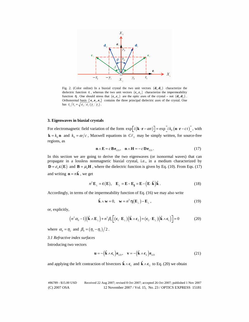
Fig. 2. (Color online) In a biaxial crystal the two unit vectors ( )1 2,d d characterize the dielectric function ε , whereas the two unit vectors ( )1 2,c c characterize the impermeability function η . One should stress that ( )1 2,c c are the optic axes of the crystal – not ( )1 2,d d . Orthonormal basis { }1 2 3, ,e e e contains the three principal dielectric axes of the crystal. One has ( )1 3 3 1 1 3τ τ ε ε γ γ= .

3. Eigenwaves in biaxial crystals

For electromagnetic field variation of the form ( ) ( )0exp expi t i k c tω⋅ − = ⋅ −⎡ ⎤ ⎡ ⎤⎣ ⎦ ⎣ ⎦k r n r , with

0k=k n and 0k cω= , Maxwell equations in 3C� may be simply written, for source-free regions, as

123 123,c c∧ = ∧ = −n E Be n H De . (17)

In this section we are going to derive the two eigenwaves (or isonormal waves) that can propagate in a lossless nonmagnetic biaxial crystal, i.e., in a medium characterized by

( )0ε=D Eε and 0μ=B H , where the dielectric function is given by Eq. (10). From Eqs. (17)

and writing ˆn=n k , we get

( ) ( )2 ˆ ˆ,n ⊥ ⊥= = − = − ⋅E E E E E E E k k�

ε . (18)

Accordingly, in terms of the impermeability function of Eq. (16) we may also write

( )2ˆ 0, n ⊥ ⊥∧ = = −k w w E Eη , (19)

or, explicitly,

( )( ) ( )( ) ( )( )2 20 0 1 2 2 1

ˆ ˆ ˆ1 0n nα β⊥ ⊥ ⊥⎡ ⎤− ∧ + ⋅ ∧ + ⋅ ∧ =⎣ ⎦

k E c E k c c E k c (20)

where 0 2α η= and ( )0 3 1 2β η η= − .

3.1 Refractive index surfaces

Introducing two vectors

( ) ( )1 123 2 123ˆ ˆ,= − ∧ = − ∧u k c e v k c e (21)

and applying the left contraction of bivectors 1ˆ ∧k c and 2

ˆ ∧k c to Eq. (20) we obtain



( ) ( ) ( ) ( )

2 2 2 20 0

1 2 2 12 20 0 0 0

,1 1

n n

n n

β βα β α β⊥ ⊥ ⊥ ⊥⋅ = ⋅ ⋅ = ⋅

− + ⋅ − + ⋅u v

c E c E c E c Eu v u v

. (22)

Whence

( )

( )4 2 2 2

0122

0 0

1 01

n

n

β

α β⊥

⎧ ⎫⎪ ⎪− ⋅ =⎨ ⎬

⎡ ⎤− + ⋅⎪ ⎪⎣ ⎦⎩ ⎭

u vc E

u v. (23)

Therefore, the eigenwaves corresponding to the direction of propagation k̂ (the wave normal) are characterized by two distinct refractive indices (birefringence) n+ and n− , such that

( )2 20 02

1

nα β

±

= + ⋅ ±u v u v . (24)

This can be readily shown to be in accordance with the results obtained using dyadic methods [17]. Nevertheless, the approach using geometric algebra is far less cumbersome than the one using dyadics. By the way, if 3, ∈a b � , then the tensor (or dyadic) product ⊗a b is such that the outer product is related to it through ∧ = ⊗ − ⊗a b a b b a . One should bear in mind, however, that bivector ∧a b has a direct geometric relation with vectors a and b whereas no such relation exists with dyadic ⊗a b .

There is a very important conclusion to be drawn from Eq. (24): for waves propagating along 1c or 2c we have, according to Eq. (21), 0=u or 0=v (respectively) and hence

20 21n α ε± = = , i.e., the two refractive indices are equal. But then, according to the definition

of optic axis, we conclude that the two unit vectors 1c and 2c that characterize the impermeability function are, in fact, the two optic axes of the biaxial crystal. We introduce two dimensionless parameters

2 1 3 2,ζ ε ε κ ε ε= = , (25)

with 1κ > and 1ζ > , in order to study the evolution of the refractive index surfaces

( )0ˆnα ± k of an anisotropic medium as shown in Fig. 3 and Fig. 4: the starting point is an

isotropic medium ( 1ζ κ= = ); then, only parameter κ is increased to obtain a uniaxial medium (parameter ζ is kept at 1ζ = ); finally, with the increase of ζ (while keeping

2.1κ = ), a biaxial medium is obtained. Only for the uniaxial case do ordinary and extraordinary waves exist, corresponding to a sphere and an ellipsoid as is well-known. For the biaxial case this clear distinction between the two eigenwaves cannot be maintained. This becomes clearer when looking at a single plane. In Fig 4 we consider the 1 2∧c c plane (i.e, the

1 3X X plane of Fig. 2): a circumference of radius 1 is always present; however, for the biaxial case, this circumference does not correspond to a single eigenwave as it is only completed through the contribution of both eigenwaves, depending on the direction under consideration.

Then we may say that, along those directions for which ( )0ˆ 1nα ± =k , an ordinary-like

behavior is found for the corresponding eigenwave – although it is not possible to distinguish anymore between ordinary and extraordinary waves as for the uniaxial case.



Fig. 3. (496 kB) The 3D refractive index surfaces, ( )0

ˆnα ± k , for the two eigenwaves of a lossless nonmagnetic crystal.

Fig. 4. (77 kB) The two refractive index surfaces, ( )0

ˆnα ± k , on the plane 1 2∧c c : surface

( )0ˆnα − k is in red and corresponds to the ordinary wave only in the uniaxial case; surface

( )0ˆnα + k is in green and corresponds to the extraordinary wave only in the uniaxial case.

3.2 Electromagnetic fields and energy velocity

From Eqs. (22) one has ( ) ( )1 2⊥ ⊥⋅ = ± ⋅v c E u c E for the two eigenwaves. Accordingly, it is

possible to define two important vectors

2 1 1 2ˆ ˆ

± = ∧ ± ∧b k c c k c c (26)

from which the electromagnetic fields for each linearly polarized eigenwave can be derived:

( ) ( )2 200 0 0 0

0

ˆ ˆ , 1n E n Eαε αε± ± ± ± ± ± ±

⎡ ⎤= ∧ = + −⎣ ⎦

D k k b E D b� , (27)



http://www.opticsexpress.org/viewmedia.cfm?URI=oe-15-23-15175-1

http://www.opticsexpress.org/viewmedia.cfm?URI=oe-15-23-15175-2

( )0 0 123ˆn

Ec

μ ±± ± ±= = − ∧B H k b e . (28)

Obviously that, when 1ˆ =k c or 2

ˆ =k c (i.e., for waves propagating along an optic axis), we

have ˆ 0±∧ =k b and these expressions fail. In fact, as is well-known, conical refraction takes place in these particular cases [2] which should be analyzed by an alternative method and will not be discussed herein. One should note that

( ) ( )2 1 1 2ˆ ˆ ˆ ˆ ˆ

±⋅ = ∧ ⋅ ± ∧ ⋅k b k c k c k c k c (29)

and hence, if k̂ is perpendicular do the plane 1 2∧c c , then ˆ 0±⋅ =k b . According to Eq. (27)

we obtain, for 20 1nα ± = ,

( ) ( )00 0

0

ˆ ˆ ˆ ˆ, E Eεα± ± ± ± ± ±

⎡ ⎤ ⎡ ⎤= = ∧ = − ⋅⎣ ⎦ ⎣ ⎦

D E E k k b b k b k� . (30)

From Eq. (27) and for ˆ 0±⋅ =k b we also get

20 0,n Eε± ± ± ± ±= =D E E b . (31)

This last result shows the meaning of the two vectors ±b : whenever ˆ±⊥k b we have an

ordinary-like behavior with both ±D and ±E parallel to ±b (respectively). In the general

biaxial case, the angles θ± between ±E and ±D (one for each eigenwave) as introduced in Eq. (4) can be explicitly obtained from

( ) ( )( ) ( )

22

22

2 2 20 0

ˆcos

ˆ2n nθ

α α

± ±

±

± ± ± ±

− ⋅=

− − ⋅

b k b

b k b. (32)

For 20 1nα ± = we just get, from Eq. (32), 0θ± = as stated previously. This same result also

occurs whenever ˆ 0±⋅ =k b . After calculating the energy density and the Poynting vector, using Eqs. (27) and (28), we derive the following expressions for the energy velocity of the two eigenwaves:

( )( ) ( ) ( )( ) ( )

( )

22 2 2

0 0

22

ˆ ˆ 1

ˆ

p p

e

n n vα α± ±± ± ± ± ± ±

±

± ±

⎡ ⎤− ⋅ − ⋅ −⎢ ⎥⎣ ⎦=

− ⋅

b k b v k b bv

b k b. (33)

The phase velocity is given by ( ) ( ) ˆp pv± ±=v k where ( )

pv c n±±= . From Eq. (33) we get

( ) ( )ˆe pv± ±⋅ =k v . (34)

This means that the phase velocity is the projection of the energy velocity along the direction

k̂ of the wave normal. From Eq. (33) we also get, for 20 1nα ± = or ˆ 0±⋅ =k b , ( ) ( )

e p± ±=v v

which reinforces our earlier statement that directions ˆ 0±⋅ =k b present an ordinary-like behavior. From Fig. 5 we can confirm that phase and energy velocities coincide when

20 1nα ± = ; for the other directions, the energy velocity is always greater than the phase



velocity. Energy velocity e ev = v is such that 3 1ev v v≤ ≤ with 1,3 1,3v c ε= (the

maximum 1v occurs on the 1X -axis and the minimum 3v on the 3X -axis); for 20 1nα ± = the

energy velocity is 2 2v c ε= . To obtain a causal medium the principal values of the

dielectric function must be above unit ( )3 2 1 1ε ε ε> > > ; otherwise the energy velocity would

be greater than the speed of light in vacuum. To study media with 1 1ε < , a causal dispersive model should be taken into account and losses included (according to the Kramers-Kronig relations); but then the two eigenwaves will not be linearly polarized anymore (the two eigenwaves will be elliptically polarized). One should stress that Eq. (33) is only valid for a lossless medium.

Fig. 5. (Color online) Normalized energy velocities ( )

2ev v± and phase velocities ( )2pv v± for

the two eigenwaves of a biaxial crystal. One has 2 0 2v c cα ε= = .

4. Conclusion

The standard approach to anisotropic media has been the coordinate method where the problem is usually solved through the principal coordinate system of the dielectric tensor as it takes, in this specific system, its simplest diagonal form. However, a coordinate-free approach is preferable as it provides solutions in their greater generality, thereby rendering the whole physical problem easier to grasp. Dyadic analysis has been the only coordinate-free method available to date – apart from differential forms which, from our perspective, do not offer any special improvements when compared to the usual dyadic approach. Nevertheless, the dyadic approach lacks a direct physical and geometrical interpretation: whenever such an interpretation is needed one usually reduces the general expressions to a specific coordinate system.

With the novel approach herein presented we have shown how geometric algebra can provide a better mathematical framework for anisotropy than tensors and dyadics. Through the direct manipulation of coordinate-free objects such as vectors, bivectors and trivectors, geometric algebra is the most natural setting to study anisotropy, providing a deeper insight and simpler calculations, without loosing its direct geometrical interpretation. We have applied our method to the problem of the electromagnetic wave propagation in biaxial crystals: the whole treatment puts in evidence the superiority of this novel approach in the determination of the two eigenwaves of these anisotropic media. In fact, as a by-product of our analysis, we have presented several new expressions that provide a better insight to the optical behavior of biaxial crystals.



Finally, with the present work, we hope to have contributed to establish a new trend in the analysis of the optics of anisotropic media by showing how Clifford’s geometric algebra may shed light on this ancient topic which, by the ongoing research on metamaterials, has regained a new interest for optical science.



anisotropy without tensors: a novel approach using ... · anisotropy without tensors: a novel...

Documents