and/or search spaces for graphical modelscsp/r126.pdf · and/or search spaces for graphical models...
TRANSCRIPT
AND/OR Search Spaces for Graphical Models
Rina Dechter and Robert Mateescu
Donald Bren School of Information and Computer ScienceUniversity of California, Irvine, CA 92697-3425
Abstract
The paper introduces an AND/OR search space perspective for graphical models that in-clude probabilistic networks (directed or undirected) and constraint networks. In contrastto the traditional (OR) search space view, the AND/OR search tree displayssome of theindependencies present in the graphical model explicitly and may sometimes reduce thesearch space exponentially. Indeed, most algorithmic advances in search-based constraintprocessing and probabilistic inference can be viewed as searching an AND/OR search treeor graph. Familiar parameters such as the depth of a spanning tree, treewidth and pathwidthare shown to play a key role in characterizing the effect of AND/OR search graphs vs. thetraditional OR search graphs. We compare memory intensive AND/OR graphsearch withinference methods, and place various existing algorithms within the AND/OR search space.
Key words: search, AND/OR search, decomposition, graphical models, Bayesiannetworks, constraint networks
1 Introduction
Bayesian networks, constraint networks, Markov random fields and influence dia-grams, commonly referred to as graphical models, are all languages for knowledgerepresentation that use graphs to capture conditional independencies between vari-ables. These independencies allow both the concise representation of knowledgeand the use of efficient graph-based algorithms for query processing. Algorithmsfor processing graphical models fall into two general types: inference-based andsearch-based. Inference-based algorithms (e.g., Variable Elimination, Tree Cluster-ing) are better at exploiting the independencies captured by the underlying graph-ical model. They provide a superior worst case time guarantee, as they are time
Email addresses:[email protected] (Rina Dechter),[email protected] (Robert Mateescu).
Preprint submitted to Elsevier Science 7 November 2006

exponential in the treewidth of the graph. Unfortunately, any method that is time-exponential in the treewidth is also space exponential in the treewidth or separatorwidth and, therefore, not practical for models with large treewidth.
Search-based algorithms (e.g., depth-first branch-and-bound, best-first search) tra-verse the model’s search space where each path represents a partial or full solu-tion. The linear structure of search spaces does not retain the independencies repre-sented in the underlying graphical models and, therefore, search-based algorithmsmay not be nearly as effective as inference-based algorithms in using this informa-tion. On the other hand, the space requirements of search-based algorithms may bemuch less severe than those of inference-based algorithms and they can accommo-date a wide spectrum of space-bounded algorithms, from linear space to treewidthbounded space. In addition, search methods require only an implicit, generative,specification of the functional relationship (given in a procedural or functionalform) while inference schemes often rely on an explicit tabular representation overthe (discrete) variables. For these reasons, search-basedalgorithms are the onlychoice available for models with large treewidth and with implicit representation.
In this paper we propose to use the well-known idea of an AND/OR search space,originally developed for heuristic search [1], to generatesearch procedures that takeadvantage of information encoded in the graphical model. Wedemonstrate how theindependencies captured by the graphical model may be used to yield AND/ORsearch trees that are exponentially smaller than the standard search tree (that canbe thought of as an OR tree). Specifically, we show that the size of the AND/ORsearch tree is bounded exponentially by the depth of a spanning pseudo tree over thegraphical model. Subsequently, we move from AND/OR search trees to AND/ORsearch graphs. Algorithms that explore the search graph involve controlled mem-ory management that allows improving their time-performance by increasing theiruse of memory. The transition from a search tree to a search graph in AND/ORrepresentations also yields significant savings compared to the same transition inthe original OR space. In particular, we show that the size ofthe minimal AND/ORgraph is bounded exponentially by the treewidth, while for OR graphs it is boundedexponentially by the pathwidth.
Our idea of the AND/OR search space is inspired by search advances introducedsporadically in the past three decades for constraint satisfaction and more recentlyfor probabilistic inference and for optimization tasks. Specifically, it resemblespseudo tree rearrangement [2,3], briefly introduced two decades ago, which wasadapted subsequently for distributed constraint satisfaction [4,5] and more recentlyin [6], and was also shown to be related to graph-based backjumping [7]. This workwas extended in [8] and more recently applied to optimization tasks [9]. Anotherversion that can be viewed as exploring the AND/OR graphs waspresented recentlyfor constraint satisfaction [10] and for optimization [11]. Similar principles were in-troduced recently for probabilistic inference (in algorithm Recursive Conditioning[12] as well as in Value Elimination [13,14]) and currently provide the backbones
2

of the most advanced SAT solvers [15]. An important contribution of this paperis in showing that all these seemingly different ideas can becast as simple traver-sal of AND/OR search spaces. We will also elaborate on the relationship betweenthis scheme and Variable Elimination [16]. We will also discuss the relationshipwith Ordered Binary Decision Diagrams (OBDD) [17], disjunctive DecomposableNegational Normal Forms (d-DNNF) and their extension to arithmetic circuits forBayesian networks [18,19], as well as with the recent work in [20–23].
The structure of the paper is as follows. Section 2 contains preliminary notationsand definitions. Section 3 describes graphical models. Section 4 introduces theAND/OR search tree that can be traversed by a linear space search algorithm. Sec-tion 5 presents the AND/OR search graph that can be traversedby memory inten-sive search algorithms. Section 6 shows how to use the AND/ORgraphs to solve areasoning problem, and gives the AND/OR search algorithm for counting and be-lief updating. Section 7 is dedicated to a detailed comparison of AND/OR searchand other new algorithmic advances in graphical models as well as compilationschemes. Finally, Section 8 provides concluding remarks. All the proofs are givenin an appendix at the end.
2 Preliminaries
Notations A reasoning problem is defined in terms of a set of variables takingvalues on finite domains and a set of functions defined over these variables. Wedenote variables or subsets of variables by uppercase letters (e.g.,X; Y; Z; S; R : : :)and values of variables by lower case letters (e.g., x; y; z; s). An assignment (X1 =x1; : : : ; Xn = xn) can be abbreviated asx = (hX1; x1i; : : : ; hXn; xni) or x =(x1; : : : ; xn). For a subset of variablesY , DY denotes the Cartesian product ofthe domains of variables inY . xY and x[Y ] are both used as the projection ofx = (x1; : : : ; xn) over a subsetY . We will also denote byY = y (or y for short) theassignment of values to variables in Y from their respectivedomains. We denotefunctions by lettersf , g, h etc., and the scope (set of arguments) of the functionfby scope(f).Definition 1 (functional operators) Given a functionh defined over a subset ofvariablesS, whereX 2 S, functions(minX h), (maxX h), and (PX h) are de-fined overU = S � fXg as follows: For everyU = u, and denoting by(u; x)the extension of tupleu by assignmentX = x, (minX h)(u) = minx h(u; x),(maxX h)(u) = maxx h(u; x), and(PX h)(u) = Px h(u; x). Given a set of func-tions h1; : : : ; hk defined over the subsetsS1; : : : ; Sk, the product function,�jhj,and summation function,
Pj hj, are defined overU = [jSj. For everyU = u,(�jhj)(u) = �jhj(uSj), and(Pj hj)(u) =Pj hj(uSj).Definition 2 (graph concepts) A directed graphis a pairG = fV;Eg, whereV =
3

fX1; : : : ; Xng is a set of vertices, andE = f(Xi; Xj)jXi; Xj 2 V g is the setof edges (arcs). If(Xi; Xj) 2 E, we say thatXi points toXj. The degree of avariable is the number of arcs incident to it. For each variable Xi, pa(Xi) or pai,is the set of variables pointing toXi in G, while the set of child vertices ofXi,denotedch(Xi), comprises the variables thatXi points to. The family ofXi, Fi,includesXi and its parent variables. A directed graph is acyclic if it has no directedcycles. Anundirected graphis defined similarly to a directed graph, but there is nodirectionality associated with the edges.
Definition 3 (induced width) An ordered graphis a pair (G; d) whereG is anundirected graph, andd = X1; : : : ; Xn is an ordering of the nodes. Thewidth ofa nodeis the number of the node’s neighbors that precede it in the ordering. Thewidth of an orderingd, is the maximum width over all nodes. Theinduced widthof an ordered graph, w�(d), is the width of the induced ordered graph obtained asfollows: nodes are processed from last to first; when nodeX is processed, all itspreceding neighbors are connected. Theinduced width of a graph, denoted byw�,is the minimal induced width over all its orderings.
Definition 4 (hypergraph) A hypergraphis a pair H = (X;S), whereS =fS1; : : : ; Stg is a set of subsets ofV calledhyperedges.
Definition 5 (tree decomposition) A tree decompositionof a hypergraphH =(X;S) is a treeT = (V;E) (V is the set of nodes, also called “clusters”, andE is the set of edges) together with a labeling function� that associates with eachvertexv 2 V a set�(v) � X satisfying:(1) For eachSi 2 S there exists a vertexv 2 V such thatSi � �(v);(2) (running intersection property)For eachXi 2 X, the setfv 2 V jXi 2 �(v)g
induces a connected subtree ofT .
Definition 6 (treewidth, pathwidth) Thewidth of a tree decomposition of a hy-pergraph is the size of its largest cluster minus 1 (maxv j�(v)j � 1). Thetreewidthof a hypergraph is the minimum width along all possible tree decompositions. Thepathwidth is the treewidth over the restricted class of chain decompositions.
It is easy to see that given an induced graph, the set of maximal cliques (also calledclusters) provide a tree decomposition of the graph, namelythe clusters can beconnected in a tree structure that satisfies the running intersection property. It iswell known that the induced width of a graph is identical to its treewidth [24]. Forvarious relationships between these and other graph parameters see [25–27].
2.1 AND/OR Search Graphs
AND/OR search spaces.An AND/OR state space representation of a problem isdefined by a 4-tuplehS;O; Sg; s0i. S is a set of states which can be either OR or
4
AND states (the OR states represent alternative ways for solving the problem whilethe AND states often represent problem decomposition into subproblems, all ofwhich need to be solved).O is a set of operators. An OR operator transforms anOR state into another state, and an AND operator transforms an AND state intoa set of states. There is a set of goal statesSg � S and a start nodes0 2 S.Example problem domains modeled by AND/OR graphs are two-player games,parsing sentences and Tower of Hanoi [1].
The AND/OR state space model induces an explicit AND/OR search graph. Eachstate is a node and its child nodes are those obtained by applicable AND or ORoperators. The search graph includes astart node. The terminal nodes (having nochild nodes) are marked as Solved (S), or Unsolved (U).
A solution subtreeof an AND/OR search graphG is a subtree which: (1) containsthe start nodes0; (2) if n in the subtree is an OR node then it contains one of itschild nodes inG and if n is an AND node it contains all its children inG; 3. allits terminal nodes are “Solved” (S). AND/OR graphs can have acost associatedwith each arc, and the cost of a solution subtree is a function(e.g., sum-cost) of thearcs included in the solution subtree. In this case we may seek a solution subtreewith optimal (maximum or minimum) cost. Other tasks that enumerate all solutionsubtrees (e.g., counting solutions) can also be defined.
3 Graphical Models
Graphical models include constraint networks defined by relations of allowed tu-ples, (directed or undirected) probabilistic networks, defined by conditional proba-bility tables over subsets of variables, cost networks defined by costs functions andinfluence diagrams which include both probabilistic functions and cost functions(i.e., utilities) [28]. Each graphical model comes with its typical queries, such asfinding a solution, or an optimal one (over constraint networks), finding the mostprobable assignment or updating the posterior probabilities given evidence, posedover probabilistic networks, or finding optimal solutions for cost networks. Thetask for influence diagrams is to choose a sequence of actionsthat maximizes theexpected utility. Markov random fields are the undirected counterparts of proba-bilistic networks. They are defined by a collection of probabilistic functions calledpotentials, over arbitrary subsets of variables. The framework presented in this pa-per is applicable across all graphical models that have discrete variables, howeverwe will draw most of our examples from constraint networks and directed proba-bilistic networks.
In general, a graphical model is defined by a collection of functionsF , over a setof variablesX, conveying probabilistic, deterministic or preferentialinformation,whose structure is captured by a graph.
5
Definition 7 (graphical models) A graphical modelR is a 4-tuple, R =hX;D; F;Ni, where:(1) X = fX1; : : : ; Xng is a set of variables;(2) D = fD1; : : : ; Dng is the set of their respective finite domains of values;(3) F = ff1; : : : ; frg is a set of real-valued functions each defined over a subset
of variablesSi � X, called its scope, and sometimes denoted byscope(fi).(4)
Ni fi 2 fQi fi;Pi fi;1i fig is a combination operator1 .
The graphical model represents the combination of all its functions:Nri=1 fi.
Next, we introduce the notion ofuniversalgraphical model which is defined by asingle function.
Definition 8 (universal equivalent graphical model) Given a graphical modelR = hX;D; F;Ni the universal equivalent model ofR is u(R) = hX;D; F =fNri=1 fig;Ni.Two graphical models areequivalent if they represent the same set of solutions.Namely, if they have the same universal model.
Definition 9 (cost of a full and a partial assignment) Given a graphical modelR, the cost of a full assignmentx = (x1; :::; xn) is defined byc(x) =Nf2F f(x[scope(f)]). Given a subset of variablesY � X, the cost of a partialassignmenty is the combination of all the functions whose scopes are included inY (FY ) evaluated at the assigned values. Namely,c(y) =Nf2FY f(y[scope(f)]).We can restrict a graphical model by conditioning on a partial assignment.
Definition 10 (conditioned graphical model) Given a graphical modelR =hX;D; F;Ni and given a partial assignmentY = y, Y � X, the conditionalgraphical model isRjy = hX;Djy; F jy;Ni, whereDjy = fDi 2 D;Xi =2 Y g andF jy = ff jY=y; f 2 F , andscope(f) 6� Y g.Consistency.For most graphical models, the functions range has a specialvalue“0” that is absorbing relative to the combination operator (e.g., multiplication).Combining anything with “0” yields a “0”. The “0” value expresses the notion ofinconsistent assignments. It is a primary concept in constraint networks but can alsobe defined relative to other graphical models that have a “0” element.
Definition 11 (consistent partial assignment, solution)Given a graphical modelhaving a “0” element, a partial assignment is consistent if its cost is non-zero. Asolution is a consistent assignment to all the variables.
Flat functions. Each function in a graphical model having a “0” element expresses1 The combination operator can also be defined axiomatically [29].
6

implicitly a constraint. Theflat constraint of functionfi is a constraintRi over itsscope that includes all and only the consistent tuples. In this paper, when we talkabout a constraint network, we refer also to the flat constraint network that canbe extracted from the general graphical model. When all the full assignments areconsistent we say that the graphical model isstrictly positive.
Unless otherwise noted, we assume that functions are expressed in a tabular explicitform, having an entry for every combination of values from the domains of theirvariables. Therefore, the specification of such functions is exponential in their scopesize (the base of the exponent is the maximum domain size). Relations, or clauses,can be expressed as functions as well, associating a value of“0” or “1” for eachtuple, depending on whether or not the tuple is in the relation (or satisfies a clause).The combination operator takes a set of functions and generates a new functionwhose scope is the union of the input functions scopes.
Definition 12 (primal graph) Theprimal graphof a graphical model is an undi-rected graph that has variables as its vertices and an edge connects any two vari-ables that appear in the scope of the same function.
Reasoning problems, queries.There are various queries/tasks that can be posedover graphical models. We refer to all asreasoning problems. In general, a reason-ing problem is a function from the graphical model to some setof elements, mostcommonly, the real numbers. We need one more functional operator,marginaliza-tion, to express most of the common queries.
Definition 13 (reasoning problem) A reasoning problemover a graphical modelis defined by a marginalization operator and a set of subsets.It is therefore a triplet,P = hR;+Y ; fZ1; : : : ; Ztgi, whereR = hX;D; F;Ni is a graphical model andZ = fZ1; : : : ; Ztg is a set of subsets of variables ofX. If S is the scope of functionf andY � X, +Y f 2 f maxS�Y f; minS�Y f; QY f; PS�Y fg, is a marginalization operator.P can be viewed as a vector function over the scopesZ1; :::; Zt. The reasoningproblem is to computePZ1;:::Zt(R):PZ1;:::Zt(R) = +Z1 rOi=1 fi; : : : ;+Zt rOi=1 fi! :We will focus primarily on reasoning problems defined byZ = ;. The marginal-ization operator is sometimes called anelimination operator because it removessome arguments from the input function’s scopes. Specifically, +Y f is defined onY . It therefore removes variablesS � Y from f ’s scope,S. Note that here
Qis the
relational projection operator and unlike the rest of the marginalization operatorsthe convention is that is defined by the scope of variables that arenoteliminated.
We next elaborate on the two popular graphical models of constraint networks andbelief networks which will be the primary focus of this paper.
7

3.1 Constraint Networks
Constraint Satisfactionis a framework for formulating real world problems, suchas scheduling and design, planning and diagnosis, and many more as a set of con-straints between variables. For example, one approach to formulating a schedulingproblem as a constraint satisfaction problem (CSP) is to create a variable for eachresource and time slice. Values of variables would be the tasks that need to bescheduled. Assigning a task to a particular variable (corresponding to a resourceat some time slice) means that this resource starts executing the given task at thespecified time. Various physical constraints (such as that agiven job takes a certainamount of time to execute, or that a task can be executed at most once) can be mod-eled as constraints between variables. Theconstraint satisfaction taskis to find anassignment of values to all the variables that does not violate any constraints, orelse to conclude that the problem is inconsistent. Other tasks are finding all solu-tions and counting the solutions.
Definition 14 (constraint network, constraint satisfaction problem) A con-straint network (CN)is defined by a 4-tuple,hX;D;C;1i, whereX is a set ofvariablesX = fX1; : : : ; Xng, associated with a set of discrete-valued domains,D = fD1; : : : ; Dng, and a set of constraintsC = fC1; : : : ; Crg. Each constraintCi is a pair (Si; Ri), whereRi is a relationRi � DSi defined on a subset ofvariablesSi � X. The relation denotes all compatible tuples ofDSi allowed by theconstraint. The combination operator,1, is join. The primal graph of a constraintnetwork is called aconstraint graph. A solution is an assignment of values to allthe variablesx = (x1; : : : ; xn), xi 2 Di, such that8 Ci 2 C, xSi 2 Ri. Theconstraint network represents its set of solutions,1i Ci.Constraint satisfactionis a reasoning problemP = hR;�; Z = ;i, whereR = hX;D;C; ./i is a constraint network, and the marginalization operator isthe projection operator�. Namely, for constraint satisfactionZ = ;, and+Y is�X�Y . So the task is to find+; Ni fi = �X ./i fi which corresponds to enumeratingall solutions. When the combination operator is a product over the cost-based rep-resentation of the relations, and the marginalization operator is logical summationwe get 1 if the constraint problem has a solution and “0” otherwise. Forcounting,the marginalization operator is summation andZ = ; too.
An immediate extension of constraint networks arecost networkswhere the set offunctions are real-valued cost functions, and the primary task is optimization.
Definition 15 (cost network, combinatorial optimization) A cost networkis de-fined by a 4-tuple,hX;D;C;Pi, whereX is a set of variablesX = fX1; : : : ; Xng,associated with a set of discrete-valued domains,D = fD1; : : : ; Dng, and a setof cost functionsC = fC1; : : : ; Crg. EachCi is a real-valued function definedon a subset of variablesSi � X. The combination operator, is
P. The reasoning
8

problem is to find a minimum or maximum cost solution which is expressed via themarginalization operator of maximization or minimization, andZ = ;.A task such as MAX-CSP: finding a solution that satisfies maximal number of con-straints (when the problem is inconsistent), can be defined by treating each relationas a cost function that assigns “0” to consistent tuples and “1” otherwise. Then thecombination operator is summation and the marginalizationoperator is minimiza-tion. Namely, the task is to find+; Ni fi = minXPi fi.3.2 Propositional Satisfiability
A special case of a CSP is thepropositional satisfiability problem(SAT). A formula' in conjunctive normal form(CNF) is a conjunction ofclauses�1; : : : ; �t wherea clause is a disjunction ofliterals (propositions or their negations). For example,� = (P _:Q_:R) is a clause, whereP ,Q andR are propositions, andP ,:Q and:R are literals. The SAT problem requires deciding whether a given CNF theoryhas amodel, i.e., a truth-assignment to its propositions that does not violate anyclause.
Propositional satisfiability (SAT) can be defined as a CSP, where propositionscorresponds to variables, domains aref0, 1g, and constraints are represented byclauses, for example clause(:A _B) is the relation (or function) over its proposi-tional variables that allows all tuples over(A;B) except(A = 1; B = 0).3.3 Belief Networks
Belief networks[30] provide a formalism for reasoning about partial beliefs underconditions of uncertainty. They are defined by a directed acyclic graph over ver-tices representing random variables of interest (e.g., the temperature of a device,the gender of a patient, a feature of an object, the occurrence of an event). The arcssignify the existence of direct causal influences between linked variables quanti-fied by conditional probabilities that are attached to each cluster of parents-childvertices in the network.
Definition 16 (belief networks)A belief network (BN)is a graphical modelP =hX;D; PG;Qi, whereX = fX1; : : : ; Xng is a set of variables over multi-valueddomainsD = fD1; : : : ; Dng. Given a directed acyclic graphG overX as nodes,PG = fPig, wherePi = fP (Xi j pa (Xi) ) g are conditional probability tables(CPTs for short) associated with eachXi, wherepa(Xi) are the parents ofXi inthe acyclic graphG. A belief network represents a probability distribution over X,P (x1; : : : ; xn) = Qni=1 P (xijxpa(Xi)). An evidence sete is an instantiated subset ofvariables.
9
When formulated as a graphical model, functions inF denote conditional proba-bility tables and the scopes of these functions are determined by the directed acyclicgraphG: each functionfi ranges over variableXi and its parents inG. The com-bination operator is
Nj = Qj. The primal graph of a belief network is called amoral graph. It connects any two variables appearing in the same CPT.
Definition 17 (belief updating) Given a belief network and evidencee, thebeliefupdatingtask is to compute the posterior marginal probability of variableXi, con-ditioned on the evidence. Namely,Bel(Xi = xi) = � Xf(x1;:::;xi�1;xi+1;:::;xn)jE=e;Xi=xig nYk=1P (xk; ejxpak);where� is a normalization constant. In this case, the marginalization operator is+Y= PX�Y , andZi = fXig. Namely,8Xi;+Xi Nk fk = PfX�XijXi=xigQk Pk.The query of finding the probability of the evidence is definedbyZ = ;.Definition 18 (most probable explanation) The most probable explanation(MPE) task is to find a complete assignment which agrees with the evidence, andwhich has the highest probability among all such assignments. Namely, to find anassignment(xo1; : : : ; xon) such thatP (xo1; : : : ; xon) = maxx1;:::;xn nYk=1P (xk; ejxpak):As a reasoning problem, an MPE task is to find+; Ni fi = maxX Qi Pi. Namely,the marginalization operator ismax andZ = ;.Markov networks are graphical models very similar to belief networks. The onlydifference is that the set of probabilistic functionsPi, called potentials, can be de-fined over any subset of variables. An important reasoning task for Markov net-works is to find the partition function which is defined by the marginalization op-erator of summation, whereZ = ;.4 AND/OR Search Trees for Graphical Models
We will next present the AND/OR search space for a generalgraphical modelstarting with an example of a constraint network.
Example 19 Consider the simple tree graphical model (i.e., the primal graph isa tree) in Figure 1(a), over domainsf1; 2; 3g, which represents a graph-coloringproblem. Namely, each node should be assigned a value such that adjacent nodes
10

X
Y Z
T R L M
(a) A constrainttree
1 2 3
2 3 1 3 1 2
1 3 1 2
X
T
R
Y
Z
L
M
2 3 1 2 2 3 1 3
1 3 1 3 1 2 1 2 1 2 1 2 2 3 2 3
2 3 2 3 2 3
1 3
1 3 1 3
(b) OR search tree
1 2 3
X
Y Z Y Z Y Z
2 32 3
T R L M
1 3 1 3 1 2 1 2
OR
OR
AND
AND
OR
AND
(c) AND/OR search tree with one ofits solution subtrees
Fig. 1. OR vs. AND/OR search trees; note the connector for AND arcs
have different values. Once variableX is assigned the value 1, the search space itroots can be decomposed into two independent subproblems, one that is rooted atYand one that is rooted at Z, both of which need to be solved independently. Indeed,givenX = 1, the two search subspaces do not interact. The same decompositioncan be associated with the other assignments toX, hX; 2i and hX; 3i. Applyingthe decomposition along the tree (in Figure 1(a) yields the AND/OR search tree inFigure 1(c). In the AND/OR space a full assignment to all the variables is not apath but a subtree. For comparison, the traditionalOR search tree is depicted inFigure 1(b). Clearly, the size of the AND/OR search space is smaller than that ofthe regular OR space. The OR search space has3 � 27 nodes while the AND/OR has3 �25 (compare 1(b) with 1(c)). Ifk is the domain size, a balanced binary tree withnnodes has an OR search tree of sizeO(kn). The AND/OR search tree, whose pseudotree has depthO(log2 n), has sizeO((2k)log2 n) = O(n � klog2 n) = O(n1+log2 k).Whenk = 2, this becomesO(n2).The AND/OR space is not restricted to tree graphical models.It only has to beguided by abackbonetree which spans the original primal graph of the graphicalmodel in a particular way. We will define the AND/OR search space relative to adepth-first search tree (DFS tree) of the primal graph first, and will generalize to abroader class of backbone spanning trees subsequently. Forcompleteness sake wedefineDFS spanning tree, next.
Definition 20 (DFS spanning tree)Given a DFS traversal ordering of an undi-rected graphG = (V;E), d = X1; : : : ; Xn, theDFS spanning treeT of G is de-fined as the tree rooted at the first node,X1, which includes only the traversed arcsofG. Namely,T = (V;E 0), whereE 0 = f(Xi; Xj) j Xj traversed from Xig.We are now ready to define the notion of AND/OR search tree for agraphicalmodel.
Definition 21 (AND/OR search tree) Given a graphical model R =11

hX;D; F;Ni, its primal graphG and a backbone DFS treeT of G, the as-sociated AND/OR search tree, denotedST (R), has alternating levels of AND andOR nodes. The OR nodes are labeledXi and correspond to the variables. The ANDnodes are labeledhXi; xii (or simplyxi) and correspond to the value assignmentsin the domains of the variables. The structure of the AND/OR search tree is basedon the underlying backbone treeT . The root of the AND/OR search tree is an ORnode labeled by the root ofT . A path from the root of the search treeST (R) to anoden is denoted by�n. If n is labeledXi or xi the path will be denoted�n(Xi) or�n(xi), respectively. The assignment sequence along path�n, denotedasgn(�n) isthe set of value assignments associated with the sequence of AND nodes along�n:asgn(�n(Xi))= fhX1; x1i; hX2; x2i; : : : ; hXi�1; xi�1ig;asgn(�n(xi))= fhX1; x1i; hX2; x2i; : : : ; hXi; xiig:The set of variables associated with OR nodes along path�n is denoted byvar(�n):var(�n(Xi)) = fX1; : : : ; Xi�1g, var(�n(xi)) = fX1; : : : ; Xig . The exact parent-child relationship between nodes in the search space are defined as follows:(1) An OR node,n, labeled byXi has a child AND node,m, labeledhXi; xii iffhXi; xii is consistent with the assignmentasgn(�n). Consistency is defined
relative to the flat constraints.(2) An AND nodem, labeledhXi; xii has a child OR noder labeledY , iff Y is
child ofX in the backbone treeT . Each OR arc, emanating from an OR toan AND node is associated with a weight to be defined shortly (see Definition26).
Clearly, if a noden is labeledXi (OR node) orxi (AND node),var(�n) is the set ofvariables mentioned on the path from the root toXi in the backbone tree, denotedbypathT (Xi) 2 .
A solution subtree is defined in the usual way:
Definition 22 (solution subtree) A solution subtreeof an AND/OR search treecontains the root node. For every OR nodes it contains one of its child nodes andfor each of its AND nodes it contains all its child nodes, and all its leaf nodes areconsistent.
Example 23 In the example of Figure 1(a),T is the DFS tree which is the treerooted atX, and accordingly the root OR node of the AND/OR tree in 1(c) isX.Its child nodes are labeledhX; 1i; hX; 2i; hX; 3i (only the values are noted in theFigure), which are AND nodes. From each of these AND nodes emanate two ORnodes,Y andZ, since these are the child nodes ofX in the DFS tree of (1(a)).The descendants ofY along the path from the root,(hX; 1i), are hY; 2i andhY; 3ionly, sincehY; 1i is inconsistent withhX; 1i. In the next level, from each nodehY; yi2 When the AND/OR tree is extended to dynamic variable orderings the set of variablesalong different paths may vary.
12

emanate OR nodes labeledT andR and fromhZ; zi emanate nodes labeledL andM as dictated by the DFS tree. In 1(c) a solution tree is highlighted.
4.1 Weights of OR-AND Arcs
The arcs in AND/OR trees are associated with weightsw that are defined based onthe graphical model’s functions and combination operator.The simplest case is thatof constraint networks.
Definition 24 (Arc weight for constraint networks) Given an AND/OR treeST (R) of a constraint networkR, each terminal node is assumed to have a sin-gle, dummy, outgoing arc. The outgoing arc of a terminal AND node always hasthe weight “1” (namely it is consistent and thus solved). An outgoing arc of a ter-minal OR node has weight “0”, (there is no consistent value assignments). Theweight of any internal OR to AND arc is “1”. The arcs from AND to OR nodeshave no weight.
We next define arc weights for any graphical model using the notion of buckets offunctions.
Definition 25 (buckets relative to a backbone tree)Given a graphical modelR = hX;D; F;Ni and a backbone treeT , the bucketof Xi relative toT , de-notedBT (Xi), is the set of functions whose scopes containXi and are included inpathT (Xi), which is the set of variables from the root toXi in T . Namely,BT (Xi) = ff 2 F jXi 2 scope(f); scope(f) � pathT (Xi)g:Definition 26 (OR-to-AND weights) Given an AND/OR treeST (R), of a graph-ical modelR, the weightw(n;m)(Xi; xi) of arc (n;m) whereXi labelsn and xilabelsm, is thecombinationof all the functions inBT (Xi) assigned by valuesalong�m. Formally,w(n;m)(Xi; xi) =Nf2BT (Xi) f(asgn(�m)[scope(f)]).Definition 27 (weight of a solution subtree)Given a weighted AND/OR treeST (R), of a graphical modelR, and given a solution subtreet having OR-to-ANDset of arcsarcs(t), the weight oft is defined byw(t) =Ne2arcs(t) w(e).Example 28 Figure 2 shows a belief network, a DFS tree that drives its weightedAND/OR search tree, and a portion of the AND/OR search tree with the appropriateweights on the arcs expressed symbolically. In this case the bucket ofE containsthe functionP (EjA;B), and the bucket ofC contains two functions,P (CjA) andP (DjB;C). Note thatP (DjB;C) belongs neither to the bucket ofB nor to thebucket ofD, but it is contained in the bucket ofC, which is the last variable in itsscope to be instantiated in a path from the root of the tree. Wesee indeed that the
13

A
C
B
DE
A
D
B C
E
0
A
B
0
E D
0 1
C
0
0 1
1
C
0 1
1
E D
0 1
C
0
0 1
1
C
0 1
P(A=0)
P(B=0|A=0) P(B=1|A=0)
P(E=0|A=0,B=0)
P(D=0|B=0,C=0)×P(C=0|A=0)
P(D=1|B=1,C=1)×P(C=1|A=0)
P(D=0|B=0,C=1)×P(C=1|A=0)
P(D=1|B=0,C=0)×P(C=0|A=0)
P(D=1|B=0,C=1)×P(C=1|A=0)
P(D=0|B=1,C=0)×P(C=0|A=0)
P(D=0|B=1,C=1)×P(C=1|A=0)
P(D=1|B=1,C=0)×P(C=0|A=0)
P(E=1|A=0,B=0) P(E=0|A=0,B=1) P(E=1|A=0,B=1)
Fig. 2. Arc weights for probabilistic networks
A
C
B
DE
A
D
B C
E
0
A
B
0
E D
0 1
C
0
0 1
1
C
0 1
1
E D
0 1
C
0
0 1
1
C
0 1
R(A=0, B=0) R(A=0,B=1)
R(A=0,B=0,E=0)
R(B=0,C=0,D=0)×R(A=0,C=0)
R(B=1,C=1,D=1)×R(A=0,C=1)
R(B=0,C=1,D=0)×R(A=0,C=1)
R(B=0,C=0,D=1)×R(A=0,C=0)
R(B=0,C=1,D=1)×R(A=0,C=1)
R(B=1,C=0,D=0)×R(A=0,C=0)
R(B=1,C=1,D=0)×R(A=0,C=1)
R(B=1,C=0,D=1)×R(A=0,C=0)
R(A=0,B=0,E=1) R(A=0,B=1,E=0) R(A=0,B=1,E=1)
R(AB)R(AC)R(ABE)R(BCD)
Fig. 3. Arc weights for constraint networks
weights on the arcs from the OR nodeE and any of its AND value assignmentsinclude only the instantiated functionP (EjA;B), while the weights on the arcsconnectingC to its AND child nodes are the products of the two functions in itsbucket instantiated appropriately. Figure 3 shows a constraint network with fourrelations, a backbone DFS tree and a portion of the AND/OR search tree withweights on the arcs. Note that the complex weights would reduce to“0”s and “1”sin this case. However, since we use the convention that arcs appear in the searchtree only if they represent a consistent extension of a partial solution, we will notsee arcs having zero weights.
4.2 Properties of AND/OR Search Tree
Any DFS treeT of a graphG has the property that the arcs ofG which are not inTare backarcs. Namely, they connect a node and one of its ancestors in the backbonetree. This ensures that each scope ofF will be fully assigned on some path inT , aproperty that is essential for the validity of the AND/OR search tree.
Theorem 29 (correctness)Given a graphical modelR having a primal graphGand a DFS spanning treeT ofG, its weighted AND/OR search treeST (R) is soundand complete, namely: 1) there is a one-to-one correspondence between solutionsubtrees ofST (R) and solutions ofR; 2) the weight of any solution tree equals thecost of the full solution it denotes; namely, ift is a solution tree ofST (R) whichdenotes a solutionx = (x1; :::xn) thenc(x) = w(t).
14

Table 1OR vs. AND/OR search size, 20 nodes
OR space AND/OR space
treewidth height time (sec.) nodes time (sec.) AND nodes OR nodes
5 10 3.154 2,097,151 0.03 10,494 5,247
4 9 3.135 2,097,151 0.01 5,102 2,551
5 10 3.124 2,097,151 0.03 8,926 4,463
5 10 3.125 2,097,151 0.02 7,806 3,903
6 9 3.124 2,097,151 0.02 6,318 3,159
The virtue of an AND/OR search tree representation is that its size may be farsmaller than the traditional OR search tree. The size of an AND/OR search treedepends on the depth of its backbone DFS treeT . Therefore, DFS trees of smallerdepth should be preferred to drive the AND/OR searchtree. An AND/OR searchtree becomes an OR search tree when its DFS tree is a chain.
Theorem 30 (size bounds of AND/OR search tree)Given a graphical modelR,with domains size bounded byk, and a DFS spanning treeT having depthm andl leaves, the size of its AND/OR search treeST (R) isO(l � km) (and therefore alsoO(nkm) andO((bk)m) whenb bounds the branching degree ofT andn boundsthe number of nodes). In contrast the size of its OR search tree along any orderingis O(kn). The above bounds are tight and realizable for fully consistent graphicalmodels. Namely, one whose all full assignments are consistent.
Table 1 demonstrates the size saving of AND/OR vs. OR search spaces for 5 ran-dom networks having 20 bivalued variables, 18 CPTs with 2 parents per child and 2root nodes, when all the assignments are consistent (remember that this is the casewhen the probability distribution is strictly positive). The size of the OR space isthe full binary tree of depth 20. The size of the full AND/OR space varies basedon the backbone DFS tree. We can give a better analytic bound on the search spacesize by spelling out the depthmi of each leaf nodeLi in T .
Proposition 31 Given a graphical modelR, with domains size bounded byk, anda backbone spanning treeT havingL = fL1; : : : ; Llg leaves, where depth of leafLi is mi, then the size of its full AND/OR search treeST (R) is O(Plk=1 kmi). Al-ternatively, we can use the exact domain sizes for each variable yielding an evenmore accurate expressionO(PLk2L�fXj jXj2pathT (Lk)gjD(Xj)j).
15

(a)
61
23
4
7 5
3
4
2
1
7
5
6
(b)
3
42
1
7
5
6
(c)
3
7
4
2
1
(d)
6
5
Fig. 4. (a) A graph; (b) a DFS treeT1; (c) a pseudo treeT2; (d) a chain pseudo treeT34.3 From DFS Trees to Pseudo Trees
There is a larger class of trees that can be used as backbones for AND/OR searchtrees, calledpseudo trees[2]. They have the above mentioned back-arc property.
Definition 32 (pseudo tree, extended graph)Given an undirected graphG =(V;E), a directed rooted treeT = (V;E 0) defined on all its nodes is apseudotreeif any arc ofG which is not included inE 0 is a back-arc inT , namely it con-nects a node inT to an ancestor inT . The arcs inE 0 may not all be included inE. Given a pseudo treeT ofG, theextended graphofG relative toT is defined asGT = (V;E [ E 0).Clearly, any DFS tree and any chain of a graph are pseudo trees.
Example 33 Consider the graphG displayed in Figure 4(a). Orderingd1 =(1; 2; 3; 4; 7; 5; 6) is a DFS ordering of a DFS treeT1 having the smallest DFStree depth of 3 (Figure 4(b)).
The treeT2 in Figure 4(c) is a pseudo tree and has a tree
depth of 2 only. The two tree-arcs (1,3) and (1,5) are not inG. TreeT3 in Figure4(d), is a chain. The extended graphsGT1 , GT2 andGT3 are presented in Figure4(b),(c),(d) when we ignore directionality and include the dotted arcs.
It is easy to see that the weighted AND/OR search tree is well defined when thebackbone trees is a pseudo tree. Namely, the properties of soundness and com-pleteness hold and the size bounds are extendible.
Theorem 34 (properties of AND/OR search trees)Given a graphical modelRand a backbone pseudo treeT , its weighted AND/OR search treeST (R) is soundand complete, and its size isO(l � km) wherem is the depth of the pseudo tree,lbounds its number of leaves, andk bounds the domain size.
Example 35 Figure 5 shows the AND/OR search trees along the pseudo treesT1andT2 from Figure 4. Here the domains of the variables arefa; b; cg and the con-
16

a
1
2
a
3
a b
4 4
b
cba a cb cba
c
4
3
a b
4 4
cba a cb cba
c
4
c
3
a b
4 4
cba a cb cba
c
4
7
a
5
a b
6 6
b
cba a cb cba
c
6
5
a b
6 6
cba a cb cba
c
6
c
5
a b
6 6
cba a cb cba
c
6
b
2
a
3
a b
4 4
b
cba a cb cba
c
4
3
a b
4 4
cba a cb cba
c
4
c
3
a b
4 4
cba a cb cba
c
4
7
a
5
a b
6 6
b
cba a cb cba
c
6
5
a b
6 6
cba a cb cba
c
6
c
5
a b
6 6
cba a cb cba
c
6
c
2
a
3
a b
4 4
b
cba a cb cba
c
4
3
a b
4 4
cba a cb cba
c
4
c
3
a b
4 4
cba a cb cba
c
4
7
a
5
a b
6 6
b
cba a cb cba
c
6
5
a b
6 6
cba a cb cba
c
6
c
5
a b
6 6
cba a cb cba
c
6
a
1
3
a
4
a b c
2
a b c
b
4
a b c
2
a b c
c
4
a b c
2
a b c
5
a
7
a b c
6
a b c
b
7
a b c
6
a b c
c
7
a b c
6
a b c
a
3
a
4
a b c
2
a b c
b
4
a b c
2
a b c
c
4
a b c
2
a b c
5
a
7
a b c
6
a b c
b
7
a b c
6
a b c
c
7
a b c
6
a b c
c
3
a
4
a b c
2
a b c
b
4
a b c
2
a b c
c
4
a b c
2
a b c
5
a
7
a b c
6
a b c
b
7
a b c
6
a b c
c
7
a b c
6
a b c
Fig. 5. AND/OR search tree along pseudo treesT1 andT2straints are universal. The AND/OR search tree based onT2 is smaller, becauseT2has a smaller depth thanT1. The weights are not specified here.
Finding good pseudo trees.Finding a pseudo tree or a DFS tree of minimal depthis known to be NP-complete. However various greedy heuristics are available. Forexample, pseudo trees can be obtained by generating a heuristically good inducedgraph along an orderingd and then traversing the induced graph depth-first, break-ing ties in favor of earlier variables [8]. For more information see [31,32].
The definition of buckets relative to a backbone tree extendsto pseudo trees as well,and this allows the definitions of weights for an AND/OR tree based on pseudo tree.Next we define the notion of abucket treeand show that it corresponds a pseudotree. This relationship will be used to make additional connections between variousgraph parameters.
Definition 36 (bucket tree [33]) Given a graphical model, its primal graphG andan orderingd, the bucket treeof G along d is defined as follows. LetG�d be theinduced graph ofG alongd. Each variableX has an associatedbucket, denotedbyBX , that containsX and its earlier neighbors in the induced graphG�d (similarto Definition 25). The nodes of the bucket tree are then buckets. Each nodeBXpoints toBY (BY is the parent ofBX) if Y is the latest earlier neighbor ofX inG�d.The following relationship between the treewidth and the depth of pseudo trees isknown [8,26]. Given atree decompositionof a primal graphG havingn nodes,whose treewidth isw�, there exists a pseudo treeT of G whose depth,m, satisfies:m � w� � logn. It can also be shown that any bucket tree [33] yields a pseudotree and that a min-depth bucket tree yields min-depth pseudo trees. The depth of abucket tree was also calledelimination depthin [26].
17

Table 2Average depth of pseudo trees vs. DFS trees; 100 instances of each random model
Model (DAG) width Pseudo tree depth DFS tree depth
(N=50, P=2, C=48) 9.5 16.82 36.03
(N=50, P=3, C=47) 16.1 23.34 40.60
(N=50, P=4, C=46) 20.9 28.31 43.19
(N=100, P=2, C=98) 18.3 27.59 72.36
(N=100, P=3, C=97) 31.0 41.12 80.47
(N=100, P=4, C=96) 40.3 50.53 86.54
In summary,
Proposition 37 [8,26] The minimal depthm over all pseudo trees satisfiesm �w� � logn, wherew� is the treewidth of the primal graph of the graphical model.
Therefore,
Theorem 38 A graphical model that has a treewidthw� has an AND/OR searchtree whose size isO(n � k(w��logn)), wherek bounds the domain size andn is thenumber of variables.
For illustration, Table 2 shows the effect of DFS spanning trees against pseudotrees, both generated using brute-force heuristics over randomly generated graphs,whereN is the number of variables,P is the number of variables in the scope of afunction andC is the number of functions.
4.4 Pruning Inconsistent Subtrees for the Flat Constraint Networks
Most advanced constraint processing algorithms incorporate no-good learning, andconstraint propagation during search, or use variable elimination algorithms suchasadaptive-consistencyanddirectional resolution[34], generating all relevant no-goods, prior to search. Such schemes can be viewed as compiling a representationthat would yield aprunedsearch tree. We next define thebacktrack-freeAND/ORsearch tree.
Definition 39 (backtrack-free AND/OR search tree) Given an AND/OR searchtree ST (R), the backtrack-free AND/OR search treeof R based onT , denotedBFT (R), is obtained by pruning fromST (R) all inconsistent subtrees, namely allnodes that root no consistent partial solution.
Example 40 Consider 5 variablesX;Y; Z; T;R over domainsf2; 3; 5g, where theconstraints are:X dividesY andZ, andY dividesT andR. The constraint graph
18

X
Y Z
T R
{2,3,5}
{2,4,7} {2,3,5}
{4,5,7} {4,6,7}
(a) A constrainttree
2 3 5
X
Y Z Y Z Y
22 4
T
4
3
Z
3
R
4
T
4
R
41 1 1 1
1 1 1
1 1 1 1
1 1
1 1 0 1 0 1
1 0 0
1
(b) Search tree
2
X
Y Z
22 4
T
4
R
4
T
4
R
4
OR
OR
AND
AND
OR
AND 1 1 1 1
1
1 1 1 1
1 1
1 1
1
1
(c) Backtrack-free searchtree
Fig. 6. AND/OR search tree and backtrack-free tree
and the AND/OR search tree relative to the DFS tree rooted atX, are given inFigure 6(a). In 6(b) we present theST (R) search space whose nodes’ consistencystatus (which will latter will be referred to asvalues) are already evaluated hav-ing value “1” is consistent and “0” otherwise. We also highlight two solutionssubtrees; one depicted by solid lines and one by dotted lines. Part (c) presentsBFT (R), where all nodes that do not root a consistent solution are pruned.
If we traverse the backtrack-free AND/OR search tree we can find a solution sub-tree without encountering any dead-ends. Some constraint networks specificationsyield a backtrack-free search space. Others can be made backtrack-free by massag-ing their representation usingconstraint propagationalgorithms before or duringsearch. In particular, it is well known that variable-elimination algorithms suchasadaptive-consistency[35] and directional resolution [36], applied in a reversedorder ofd (whered is the DFS order of the pseudo tree) compile a constraint spec-ification (resp., a Boolean CNF formula) that has a backtrack-free search space.Assuming that the reader is familiar with variable elimination algorithms [16] wedefine:
Definition 41 (directional extension [35,36])LetR be a constraint problem andlet d be a DFS traversal ordering of a backbone pseudo tree of its primal graph,then we denote byEd(R) the constraint network (resp., the CNF formula) compiledby Adaptive-consistency (resp., directional resolution)in reversed order ofd.
Proposition 42 Given a Constraint networkR, the AND/OR search tree of thedirectional extensionEd(R) whend is a DFS ordering ofT , is identical to thebacktrack-free AND/OR search tree ofR based onT . NamelyST (Ed(R)) =BFT (R).Example 43 In Example 40, if we apply adaptive-consistency in reverse order ofX;Y; T;R; Z, the algorithm will remove the values3; 5 from the domains of bothXandZ yielding a tighter constraint networkR0. The AND/OR search tree in Figure
19

40(c) is bothST (R0) andBFT (R).Proposition 42 emphasizes the significance of no-good learning [37] for decid-ing inconsistency or for finding a single solution. These techniques are known asclause learning in SAT solvers, first introduced by [38] and are currently used inmost advanced solvers [39]. Namely, when we apply no-good learning we explorethe search space whose many inconsistent subtrees are pruned. For counting how-ever, and for other relevant tasks, pruning inconsistent subtrees and searching thebacktrack-free search tree yields a partial help only, as weelaborate later.
5 AND/OR Search Graphs
It is often the case that a search space that is a tree can become a graph if identicalnodes are merged, because identical nodes root identical search subspaces, andcorrespond to identical reasoning subproblems. Any two nodes that root identicalweighted subtrees can bemerged, reducing the size search graph. For example, inFigure 1(c), the search trees below any appearance ofhY; 2i are all identical, andtherefore can be merged.
Sometimes, two nodes may not root identical subtrees, but they could still rootsearch subspaces that correspond to equivalent subproblems. Nodes that root equiv-alent subproblems having the same universal model (see Definition 44) even thoughthe weighted subtrees may not be identical, can beunified, yielding an even smallersearch graph, as we will show.
We next formalize the notions ofmergingandunifyingnodes and define the mini-mal AND/OR search graph.
5.1 Minimal AND/OR Search Graphs
An AND/OR search tree can also be viewed as a data structure that defines auniver-sal graphical model (see Definition 8), defined by the weights of its set of solutionsubtrees (see Definition 22).
Definition 44 (universal graphical model of AND/OR search trees) Given aweighted AND/OR search treeG over a set of variablesX and domainsD, itsuniversal graphical model, denoted byU(G), is defined by its set of solutionsas follows: if t is a solution subtree andx = asgn(t) is the set of assignmentsassociated witht thenu(x) = w(t); otherwiseu(x) = 0.
A graphical modelR is equivalent to its AND/OR search tree,ST (R), which meansthatu(R) is identical toU(ST (R)). We will next define sound merge operations
20

C
A
B
C
A B
0
C
A
0
B
0 1
1
B
0 1
1
A
0
B
0 1
1
B
0 1
(a) (b) (c)
20111
15011
2101
1001
4110
3010
6100
3000
f(C,A,B)BAC
111
601
510
200
f(C,A)AC
2 5 6 1
3 6 3 4 1 2 15 20
6 12 15 20 6 12 15 20
Fig. 7. Merge vs. unify operators
that transform AND/OR search trees into graphs that preserve equivalence.
Definition 45 (merge) Assume a given weighted AND/OR search graphS 0T (R)(S 0T (R) can be the AND/OR search treeST (R)), and assume two paths�1 =�n1(xi) and�2 = �n2(xi) ending by AND nodes at leveli having the same labelxi. Nodesn1 and n2 can bemergediff the weighted search subgraphs rooted atn1 andn2 are identical. Themergeoperator,merge(n1; n2), redirects all the arcsgoing inton2 into n1 and removesn2 and its subgraph. It thus transformsS 0T intoa smaller graph. When we merge AND nodes only we call the operation AND-merge. The same reasoning can be applied to OR nodes, and we call the operationOR-merge.
We next define the semantic notion ofunifiablenodes, as opposed to the syntacticdefinition ofmerge.
Definition 46 (unify) Given a weighted AND/OR search graphG for a graphicalmodelR and given two paths�n1 and�n2 having the same label on nodesn1 andn2, thenn1 andn2 are unifiable, iff they root equivalent conditioned subproblems(Definition 10). Namely, ifRjasgn(�1) = Rjasgn(�2).Example 47 Let’s follow the example in Figure 7 to clarify the difference betweenmergeand unify. We have a graphical model defined by two functions (e.g.costfunctions) over three variables. The search tree given in Figure 7(c) cannot bereduced to a graph bymerge, because of the different arc weights. However, thetwo OR nodes labeledA root equivalent conditioned subproblems (the cost of eachindividual solution is given at the leaves). Therefore, thenodes labeledA can beunified, but they cannot be recognized as identical by themergeoperator.
Proposition 48 (minimal graph) Given a weighted AND/OR search graphGbased on pseudo treeT :(1) The merge operator has a unique fix point, called themerge-minimal
AND/OR search graph and denoted byMmergeT (G).(2) Theunify operator has a unique fix point, called theunify-minimal AND/OR
21
1 2 3
2 3 1 3 1 2
1 3 1 2
X
T
R
Y
Z
L
M
2 3 1 2 2 3 1 3
1 3 1 3 1 2 1 2 1 2 1 2 2 3 2 3
2 3 2 3 2 3
1 3
1 3 1 3
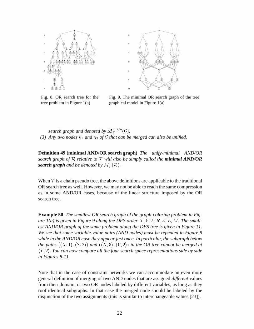
Fig. 8. OR search tree for thetree problem in Figure 1(a)
1 2 3
2 3 1 3 1 2
1 3 1 2
X
T
R
Y
Z
L
M
2 3 1 2 2 3 1 3
1 32 1 2 3
123
1 2
1 2
2 3 1
1 3
3
2 3
Fig. 9. The minimal OR search graph of the treegraphical model in Figure 1(a)
search graph and denoted byMunifyT (G).(3) Any two nodesn1 andn2 of G that can be merged can also be unified.
Definition 49 (minimal AND/OR search graph) The unify-minimal AND/ORsearch graph ofR relative toT will also be simply called theminimal AND/ORsearch graph and be denoted byMT (R).WhenT is a chain pseudo tree, the above definitions are applicable to the traditionalOR search tree as well. However, we may not be able to reach thesame compressionas in some AND/OR cases, because of the linear structure imposed by the ORsearch tree.
Example 50 The smallest OR search graph of the graph-coloring problem in Fig-ure 1(a) is given in Figure 9 along the DFS orderX;Y; T;R; Z; L;M . The small-est AND/OR graph of the same problem along the DFS tree is givenin Figure 11.We see that some variable-value pairs (AND nodes) must be repeated in Figure 9while in the AND/OR case they appear just once. In particular, the subgraph belowthe paths(hX; 1i; hY; 2i) and (hX; 3i; hY; 2i) in the OR tree cannot be merged athY; 2i. You can now compare all the four search space representations side by sidein Figures 8-11.
Note that in the case of constraint networks we can accommodate an even moregeneral definition of merging of two AND nodes that are assigneddifferentvaluesfrom their domain, or two OR nodes labeled by different variables, as long as theyroot identical subgraphs. In that case the merged node should be labeled by thedisjunction of the two assignments (this is similar to interchangeable values [23]).
22

1 2 3
X
Y Z Y Z Y Z
2 32 3
T R L M
1 3 1 3 1 2 1 2
OR
OR
AND
AND
OR
AND
Fig. 10. AND/OR search treefor the tree problem in Figure1(a)
1 2 3
X
Y Z Y Z Y Z
2 32 3
T R
1 3
1 1
2
T R T R
1 32
L M
1 32
L M L M
1 32
Fig. 11. The minimal AND/OR search graph ofthe tree graphical model in Figure 1(a)
5.2 Building AND/OR search graphs
In this subsection we will discuss practical algorithms forgenerating compactAND/OR search graphs of a given graphical model. In particular we will iden-tify effective rules for recognizing unifiable nodes, aiming towards the minimalAND/OR search graph as much as computational resources allow. The rules allowgenerating a small AND/OR graph calledthe context minimal graphwithout cre-ating the whole search treeST first. We focus first on AND/OR search graphs ofgraphical models having no cycles, calledtree models(i.e., the primal graph is atree).
5.2.1 Building AND/OR search graphs for Tree Models and Tree Decompositions
Consider again the graph in Figure 1(a) and its AND/OR search tree in Figure1(c) representing a constraint network. Observe that at level 3, nodehY; 1i appearstwice, (and so arehY; 2i andhY; 3i). Clearly however, the subtrees rooted at eachof these two AND nodes are identical and we can reason that they can be mergedbecause any specific assignment toY uniquely determines its rooted subtree. In-deed, the AND/OR search graph in Figure 11 is equivalent to the AND/OR searchtree in Figure 8 (same as Figure 1(c)).
Definition 51 (explicit AND/OR graphs for constraints tree models) Given atree model constraint network and the pseudo treeT identical to its primal graph,theexplicit AND/OR search graphof the tree model relative toT is obtained fromST by merging all AND nodes having the same labelhX; xi.Proposition 52 Given a rooted tree modelT : (1) Its explicit AND/OR searchgraphis equivalent toST . (2) The size of the explicit AND/OR search graph isO(nk). (3)For some tree models the explicit AND/OR search graph is minimal.
23

The notion of explicit AND/OR search graph for a tree model isextendable to anygeneral graphical models that are trees. The only difference is that the arcs haveweights. Thus, we need to show that merged nodes via the rule in definition 51 rootidentical weighted AND/OR trees.
Proposition 53 Given a general graphical model whose graph is a treeT , its ex-plicit AND/OR searchgraphis equivalent toST , and its size isO(nk);Next, the question is how to identifyefficientlymergeable nodes forgeneralnon-tree graphical models. A guiding idea is to transform a graphical model into a treedecomposition first, and then apply the explicit AND/OR graph construction to theresulting tree decomposition. The next paragraph sketchesthis intuition.
A tree decomposition[33] (see Definition 5) of a graphical model partitions thefunctions into clusters. Each cluster corresponds to a subproblem that has a set ofsolutions and the clusters interact in a tree-like manner. Once we have a tree de-composition of a graphical model, it can be viewed as a regular (meta) tree modelwhere each cluster is a node and its domain is the cross product of the domains ofvariables in the cluster. The constraint between two adjacent nodes in the tree de-composition is equality over the common variables. For moredetails about tree de-compositions see [33]. For the meta-tree model the explicitAND/OR search graphis well defined: the OR nodes are the scopes of clusters in the tree decomposi-tion and the AND nodes, are their possible value assignments. Since the graphicalmodel is converted into a tree, its explicit AND/OR search graph is well definedand we can bound its size.
Theorem 54 Given a tree decompositionof a graphical model, whose domainsizes are bounded byk, the explicit AND/OR search graphimplied by the treedecomposition has a size ofO(rkw�), wherer is the number of clusters in the treedecomposition andw� is the size of the largest cluster.
The tree decomposition can guide an algorithm for generating an AND/OR searchgraph whose size is bounded exponentially by the induced width, which we willrefer to in the next section as thecontext minimal graph.
While the idea of explicit AND/OR graph based on a tree decomposition can be ex-tended to any graphical model it is somewhat cumbersome. Instead, in the next sec-tion we propose a more direct approach for generating the context minimal graph.
5.2.2 The Context Based AND/OR Graph
We will now present a generative rule for merging nodes in theAND/OR searchgraph that yields the size bound suggested above. We will need the notion ofin-duced width of a pseudo tree of Gfor bounding the size of the AND/OR searchgraphs. We denote bydDFS(T ) a linear DFS ordering of a treeT .
24

Definition 55 (induced width of a pseudo tree)The induced width ofG relativeto the pseudo treeT , wT (G), is the induced width along thedDFS(T ) ordering ofthe extended graph ofG relative toT , denotedGT .
Proposition 56 (1) The minimal induced width ofG over all pseudo trees is iden-tical to the induced width (treewidth),w�, of G. (2) The minimal induced widthrestricted to chain pseudo trees is identical to its pathwidth, pw�.Example 57 In Figure 4(b), the induced graph ofG relative toT1 contains also theinduced arcs (1,3) and (1,5) and its induced width is 2.GT2 is already triangulated(no need to add induced arcs) and its induced width is 2 as well.GT3 has the addedarc (4,7) and when ordered it will have the additional induced arcs (1,5) and (1,3)edges, yielding induced width 2 as well.
We will now provide definitions that will allow us to identifynodes that can bemerged in an AND/OR graph. The idea is to find a minimal set of variable as-signments from the current path that will always generate the same conditionedsubproblem, regardless of the assignments that are not included in this minimal set.Since the current path for an OR nodeXi and an AND nodehXi; xii differ by theassignment ofXi to xi (Definition 2), the minimal set of assignments that we wantto identify will be different forXi and forhXi; xii. In the following two definitionsancestors and descendants are with respect to the pseudo treeT , while connectionis with respect to the primal graphG.
Definition 58 (parents) Given a primal graphG and a pseudo treeT of a rea-soning problemP, theparentsof an OR nodeXi, denoted bypai or paXi , are theancestors ofXi that have connections inG toXi or to descendants ofXi.Definition 59 (parent-separators) Given a primal graphG and a pseudo treeTof a reasoning problemP, theparent-separatorsof Xi (or of hXi; xii), denoted bypasi or pasXi , are formed byXi and its ancestors that have connections inG todescendants ofXi.It follows from these definitions that the parents ofXi, pai, separate in the primalgraphG (and also in the extended graphGT and in the induced extended graphGT �) the ancestors (inT ) of Xi, fromXi and its descendants (inT ). Similarly, theparents separators ofXi, pasi, separate the ancestors ofXi from its descendants.It is also easy to see that each variableXi and its parentspai form a clique in theinduced graphGT �. The following proposition establishes the relationship betweenpai andpasi.Proposition 60 (1) If Y is the single child ofX in T , thenpasX = paY .(2) If X has childrenY1; : : : ; Yk in T , thenpasX = [ki=1paYi .
Theorem 61 (context based merge)GivenGT �, let �n1 and�n2 be any two par-tial paths in an AND/OR search graph, ending with two nodes,n1 andn2.
25

(1) If n1 andn2 are AND nodes annotated byhXi; xii andasgn(�n1)[pasXi ] = asgn(�n2)[pasXi ] (1)
then the AND/OR search subtrees rooted byn1 andn2 are identical andn1andn2 can be merged.asgn(�ni)[pasXi ] is called theAND context of ni.
(2) If n1 andn2 are OR nodes annotated byXi andasgn(�n1)[paXi ] = asgn(�n2)[paXi ] (2)
then the AND/OR search subtrees rooted byn1 andn2 are identical andn1andn2 can be merged.asgn(�ni)[paXi ] is called theOR context of ni.
Example 62 For the balanced tree in Figure 1 consider the chainpseudo tree d = (X;Y; T;R; Z; L;M). Namely the chain has arcsf(X;Y ); (Y; T ); (T;R); (R;Z); (Z;L); (L;M)g and the extended graph in-cludes also the arcs(Z;X); (M;Z). The parent-separator ofT alongd is XY T(since the induced graph has the arc(T;X)), ofR it is XR, for Z it is Z and forM it is M . Indeed in the first 3 levels of the OR search graph in Figure 9 there areno merged nodes. In contrast, if we consider the AND/OR ordering along the DFStree, the parent-separator of every node is itself yieldinga single appearance ofeach AND node having the same assignment annotation in the minimal AND/ORgraph.
Definition 63 (context minimal AND/OR search graph) The AND/OR searchgraph ofR based on the backbone treeT that is closed under context-based mergeoperator is calledcontext minimalAND/OR search graph and is denotedCT (R).We should note that we can in general merge nodes based both onAND and ORcontexts. However, Proposition 60 shows that doing just oneof them renders theother unnecessary (up to some small constant factor). In practice, we would recom-mend just the OR context based merging, because it has a slight (albeit by a smallconstant factor) space advantage. In the examples that we give in this paper,CT (R)refers to an AND/OR search graph for which either the AND context based or ORcontext based merging was performed exhaustively.
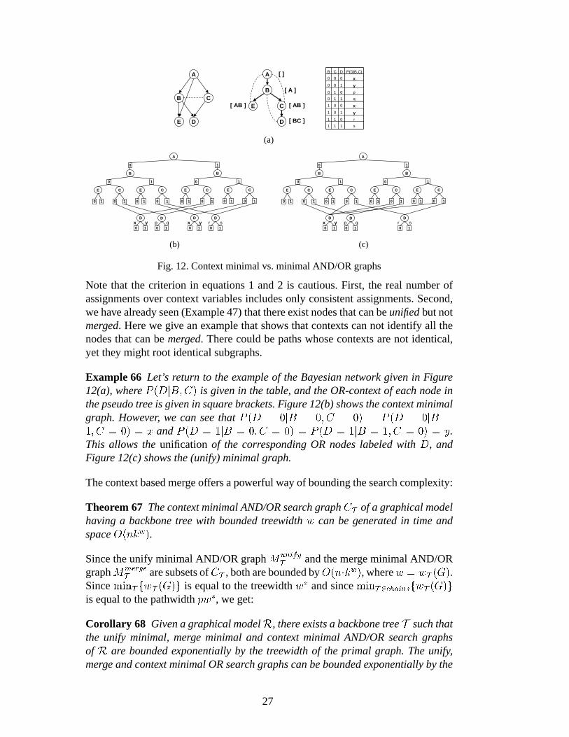
Example 64 Consider the example given in Figure 12(a). The OR context of eachnode in the pseudo tree is given in square brackets. The context minimal AND/ORsearch graph (based on OR merging) is given in Figure 12(b).
Since the number of nodes in the context minimal AND/OR search graph cannotexceed the number of different contexts, we can bound the size of the context min-imal graph.
Theorem 65 Given a graphical modelR, its primal graphG, and a pseudo treeThaving induced widthw = wT (G), the size of the context minimal AND/OR searchgraph based onT , CT (R), isO(n � kw), whenk bounds the domain size.
26
A
D
B
CE
A
D
B C
Es111
r011
y101
x001
q110
p010
y100
x000
P(D|B,C)DCB
(a)
[ ]
[ A ]
[ AB ]
[ BC ]
[ AB ]
(b)
0
A
B
0
E C
0 1
D
0 1
0 1
D
0 1
1
E C
0 1
D
0 1
0 1
D
0 1
1
B
0
E C
0 1 0 1
1
E C
0 1 0 1
x y p q r sx y
(c)
0
A
B
0
E C
0 1
D
0 1
0 1
D
0 1
1
E C
0 1 0 1
D
0 1
1
B
0
E C
0 1 0 1
1
E C
0 1 0 1
x y p q r s
Fig. 12. Context minimal vs. minimal AND/OR graphs
Note that the criterion in equations 1 and 2 is cautious. First, the real number ofassignments over context variables includes only consistent assignments. Second,we have already seen (Example 47) that there exist nodes thatcan beunifiedbut notmerged. Here we give an example that shows that contexts can not identify all thenodes that can bemerged. There could be paths whose contexts are not identical,yet they might root identical subgraphs.
Example 66 Let’s return to the example of the Bayesian network given in Figure12(a), whereP (DjB;C) is given in the table, and the OR-context of each node inthe pseudo tree is given in square brackets. Figure 12(b) shows the context minimalgraph. However, we can see thatP (D = 0jB = 0; C = 0) = P (D = 0jB =1; C = 0) = x andP (D = 1jB = 0; C = 0) = P (D = 1jB = 1; C = 0) = y.This allows theunification of the corresponding OR nodes labeled withD, andFigure 12(c) shows the (unify) minimal graph.
The context based merge offers a powerful way of bounding thesearch complexity:
Theorem 67 The context minimal AND/OR search graphCT of a graphical modelhaving a backbone tree with bounded treewidthw can be generated in time andspaceO(nkw).Since the unify minimal AND/OR graphMunifyT and the merge minimal AND/ORgraphMmergeT are subsets ofCT , both are bounded byO(n�kw), wherew = wT (G).SinceminT fwT (G)g is equal to the treewidthw� and sinceminT 2chainsfwT (G)gis equal to the pathwidthpw�, we get:
Corollary 68 Given a graphical modelR, there exists a backbone treeT such thatthe unify minimal, merge minimal and context minimal AND/OR search graphsof R are bounded exponentially by the treewidth of the primal graph. The unify,merge and context minimal OR search graphs can be bounded exponentially by the
27

pathwidth only.
5.2.3 More on OR vs. AND/OR
It is well known [26] that for any graphw� � pw� � w� � logn. It is easy to placem� (the minimal depth over pseudo trees) in that relation yielding w� � pw� �m� � w� � logn. It is also possible to show that there exist primal graphs for whichthe upper bound on pathwidth is attained, that ispw� = O(w� � logn).Consider a complete binary tree of depthm. In this case,w� = 1, m� = m, and itis also known [40,41]) that:
Theorem 69 ([41]) If T is a binary tree of depthm thenpw�(T ) � m2 .
Theorem 69 shows that for graphical models having a bounded tree widthw, theminimal AND/OR graph is bounded byO(nkw) while the minimal OR graph isbounded byO(nkw�logn). Therefore, even when caching, the use of an AND/ORvs. an OR search space can yield a substantial saving.
Remark 70 We have seen that AND/ORtreesare characterized by thedepthofthe pseudo trees while minimal AND/ORgraphsare characterized by theirinducedwidth. It turns out however that sometimes a pseudo tree that is optimal relative tow is far from optimal form and vice versa. For example a primal graph model thatis a chain has a pseudo tree havingm1 = n andw1 = 1 on one hand, and anotherpseudo tree that is balanced havingm2 = logn andw2 = logn. There is no singlepseudo tree having bothw = 1 andm = logn for a chain. Thus, if we plan tohave linear space search we should pick one kind of a backbone pseudo tree, whileif we plan to search a graph, and therefore cache some nodes, another pseudo treeshould be used.
5.3 On the Canonicity and Generation of the Minimal AND/OR Graph
We showed that the merge minimal AND/OR graph is unique for a given graphicalmodel, given a backbone pseudo tree (Proposition 48). In general, it subsumes theminimal AND/OR graph, and sometimes can be identical to it. For constraint net-works we will now prove a more significant property of uniqueness relative to allequivalent graphical models given a backbone tree. We will prove this notion rel-ative tobacktrack-freesearch graphs which are captured by the notion of stronglyminimal AND/OR graph. Remember that any graphical model can have an associ-ated flat constraint network.
Definition 71 (strongly minimal AND/OR graph) 3 A strongly minimal3 The minimal graph is built by lumping together “unifiable” nodes, which are those that
28

AND/OR graph ofR relative to a pseudo treeT is the minimal AND/OR graph,MT (R), that is backtrack-free (i.e. any partial assignment in the graph leads toa solution), denoted byM�T (R). The strongly context minimal graph is denotedC�T (R).5.3.1 Canonicity of Strongly Minimal AND/OR Search Graphs
We briefly discuss here the canonicity of the strongly minimal graph, focusingon constraint networks. Given two equivalent constraint networks representing thesame set of solutions, where each may have a different constraint graph, are theirstrongly minimal AND/OR search graphs identical?
The above question is not well defined however, because an AND/OR graph forR is defined only with respect to a backbone pseudo tree. We can have twoequivalent constraint networks having two different graphs where a pseudo treefor one graph may not be a pseudo tree for the other. Consider, for example aconstraint network having three variables:X, Y andZ and equality constraints.The following networks,R1 = fRXY = (X = Y ); RY Z = (Y = Z)gandR2 = fRXZ = (X = Z); RY Z = (Y = Z)g andR3 = fRXY =(X = Y ); RY Z = (Y = Z); RXZ = (X = Z)g are equivalent. However,T1 = (X Y ! Z) is a pseudo tree forR1, but not forR2 neither forR3. We asktherefore a different question: given two equivalent constraint networks and givena backbone tree that is a pseudo tree for both, is the stronglyminimal AND/ORgraph relative toT unique?
We will answer this question positively quite straightforwardly. We first showthat equivalent networks that share a backbone tree have identical backtrack-freeAND/OR search trees. Since the backtrack-free search treesuniquely determinetheir strongly minimal graph the claim follows.
Definition 72 (shared pseudo trees)Given a collection of graphs on the same setof nodes, we say that the graphs share a treeT , if T is a pseudo tree of each ofthese graphs. A set of graphical models defined over the same set of variables sharea treeT , iff their respective primal graphs shareT .
Proposition 73 1. IfR1 andR2 are two equivalent constraint networks that shareT , thenBFT (R1) = BFT (R2) (see Definition 39). 2. IfR1 andR2 are two equiv-alent graphical models (not necessarily constraint networks) that shareT , thenBFT (R1) = BFT (R2) as AND/OR search trees although their arcs may not haveidentical weights.
root equivalent subproblems. Therefore, at each level (corresponding to one variable), allthe nodes that root inconsistent subproblems will be unified. If we eliminate the redundantnodes, the minimal graph is already backtrack free.
29

Theorem 74 If R1 andR2 are two equivalent constraint networks that shareT ,thenM�T (R1) = M�T (R2).Theorem 74 implies thatM�T is a canonical representation of a constraint networkR relative toT .
Generating the strongly minimal AND/OR graphs
From the above discussion we see that several methods for generating the canon-ical AND/OR graph of a given graphical model, or a given AND/OR graph mayemerge. The method we focused on in this paper is to generate the context minimalAND/OR graph first. Then we can process this graph from leavesto root, whilecomputing the value of nodes, and additional nodes can be unified or pruned (iftheir value is “0”).
There is another approach that is based on processing the functions in a variableelimination style, when viewing the pseudo tree as a bucket tree or a cluster tree.The original functions can be expressed as AND/OR graphs andthey will be com-bined pairwise until an AND/OR graph is generated. This phase allows computingthe value of each node and therefore allows for semantic unification. Subsequentlya forward phase will allow generating the backtrack-free representation as well asallow computing the full values associated with each node. The full details of thisapproach are out of the scope of the current paper. For initial work restricted toconstraint networks see [42].
5.4 Merging and Pruning: Orthogonal Concepts
Notice that the notion of minimality is orthogonal to that ofpruning inconsistentsubtrees (yielding the backtrack-free search space). We can merge two identicalsubtrees whose root value is “0” but still keep their common subtree. However,since our convention is that we don’t keep inconsistent subtrees we should com-pletely prune them, irrespective of them rooting identicalor non-identical subtrees.Therefore, we can have a minimal search graph that isnotbacktrack-free as well asa non-minimal search graph (e.g.a tree) that is backtrack-free.
When the search space is backtrack-free and if we seek a singlesolution, the sizeof the minimal AND/OR search graph and its being OR vs. AND/ORare both ir-relevant. It will, however, affect a traversal algorithm that counts all solutions orcomputes an optimal solution as was often observed [43]. Forcounting and foroptimization tasks, even when we record all no-goods and cache all nodes by con-text, the impact of the AND/OR graph search vs. the OR graph search can still besignificant.
Example 75 Consider the graph problem in Figure 6(a) when we add the value 4
30

to the domains ofX andZ. Figure 13(a) gives the full AND/OR search tree andFigure 13(b) gives the backtrack-free search tree. Figure 14(a) gives the contextminimal but unpruned search graph and Figure 14(b) gives theminimal and prunedsearch graph.
X
2
Y
2
T
74 5
R
74 6
4
T
74 5
R
74 6
7
T
74 5
R
74 6
Z
2 3 4 5
3
Y
2
T
74 5
R
74 6
4
T
74 5
R
74 6
7
T
74 5
R
74 6
Z
2 3 4 5
4
Y
2
T
74 5
R
74 6
4
T
74 5
R
74 6
7
T
74 5
R
74 6
Z
2 3 4 5
5
Y
2
T
74 5
R
74 6
4
T
74 5
R
74 6
7
T
74 5
R
74 6
Z
2 3 4 5
(a) Full AND/OR tree
X
2
Y
2
T
4
R
4 6
4
T
4
R
4
Z
2 4
4
Y
4
T
4
R
4
Z
4
(b) Pruned backtrack-free AND/OR tree
Fig. 13. AND/OR treesX
2
Y
2
T
74 5
R
74 6
4
T R
7
T R
Z
2 3 4 5
3
Y Z
4
Y Z
5
Y Z
(a) Context minimal unpruned AND/OR graph
X
2
Y
2
T
4
R
4 6
4
T R
Z
2 4
4
Y Z
(b) Context minimalpruned backtrack-freeAND/OR graph
Fig. 14. AND/OR graphs
5.5 Using Dynamic Variable Ordering
The AND/OR search tree we defined uses a fixed variable ordering. It is knownthat exploring the search space in a dynamic variable ordering is highly beneficial.AND/OR search trees for graphical models can also be modifiedto allow dynamicvariable ordering. A dynamic AND/OR tree that allows variedvariable orderinghas to satisfy that for every subtree rooted by the current path �, any arc of theprimal graph that appears as a cross-arc (not a back-arc) in the subtree must be“inactive” conditioned on�.
Example 76 Consider the propositional formulaX ! A _ C andX ! B _ C.The constraint graph is given in Figure 15(a) and a DFS tree in15(b). However,the constraint subproblem conditioned onhX; 0i, has no real constraint betweenA;B;C, so the effective spanning tree belowhX; 0i is fhX; 0i ! A; hX; 0i !B; hX; 0i ! Cg, yielding the AND/OR search tree in Figure 15(c). Note that whilethere is an arc betweenA andC in the constraint graph, the arc isnotactive whenX is assigned the value0.
31
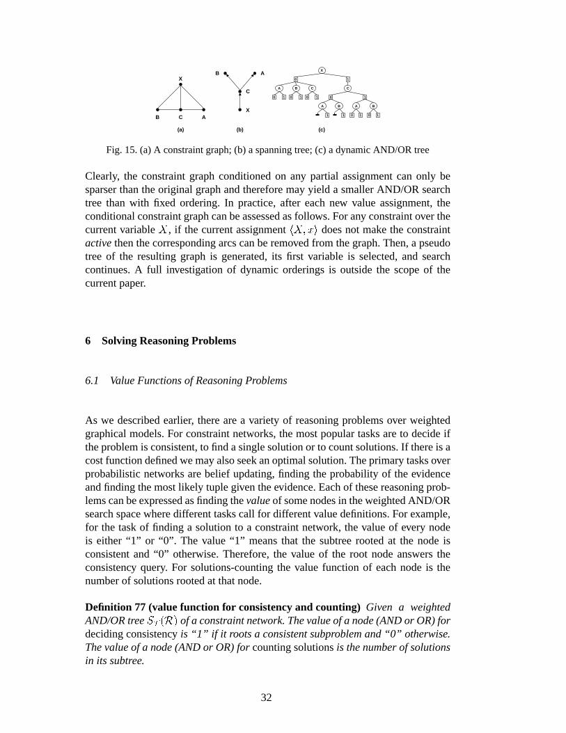
CB
X
A
(a)
AB
C
X
(b) (c)
X
1
A C
0
A
1
B
1
1
A
0 1
B
0 1
0 1
0
B
0 1
C
0 1
Fig. 15. (a) A constraint graph; (b) a spanning tree; (c) a dynamic AND/OR tree
Clearly, the constraint graph conditioned on any partial assignment can only besparser than the original graph and therefore may yield a smaller AND/OR searchtree than with fixed ordering. In practice, after each new value assignment, theconditional constraint graph can be assessed as follows. For any constraint over thecurrent variableX, if the current assignmenthX; xi does not make the constraintactivethen the corresponding arcs can be removed from the graph. Then, a pseudotree of the resulting graph is generated, its first variable is selected, and searchcontinues. A full investigation of dynamic orderings is outside the scope of thecurrent paper.
6 Solving Reasoning Problems
6.1 Value Functions of Reasoning Problems
As we described earlier, there are a variety of reasoning problems over weightedgraphical models. For constraint networks, the most popular tasks are to decide ifthe problem is consistent, to find a single solution or to count solutions. If there is acost function defined we may also seek an optimal solution. The primary tasks overprobabilistic networks are belief updating, finding the probability of the evidenceand finding the most likely tuple given the evidence. Each of these reasoning prob-lems can be expressed as finding thevalueof some nodes in the weighted AND/ORsearch space where different tasks call for different valuedefinitions. For example,for the task of finding a solution to a constraint network, thevalue of every nodeis either “1” or “0”. The value “1” means that the subtree rooted at the node isconsistent and “0” otherwise. Therefore, the value of the root node answers theconsistency query. For solutions-counting the value function of each node is thenumber of solutions rooted at that node.
Definition 77 (value function for consistency and counting)Given a weightedAND/OR treeST (R) of a constraint network. The value of a node (AND or OR) fordeciding consistencyis “1” if it roots a consistent subproblem and “0” otherwise.The value of a node (AND or OR) forcounting solutionsis the number of solutionsin its subtree.
32

It is easy to see that the value of nodes in the search graph canbe computed recur-sively from leaves to root.
Proposition 78 (recursive value computation)(1) For the consistency task thevalue of AND leaves is their labels and the value of OR leaves is“0” (they areinconsistent). An internal OR node is labeled “1” if one of its successor nodes is“1” and an internal AND node has value “1” iff all its successorOR nodes havevalue “1”.(2) The counting values of leaf AND nodes are “1” and of leaf OR nodes are “0”.The counting value of an internal OR node is the sum of the counting-values of allits child nodes. The counting-value of an internal AND node isthe product of thecounting-values of all its child nodes.
We can now generalize to any reasoning problem, focusing on the simplified casewhenZ = ;, namely when the marginalization has to be applied to all thevariables.This special case captures most tasks of interest. We will start with the recursivedefinition.
Definition 79 (recursive definition of values) The value function of a reasoningproblemP = hR;+Y ; Zi, whereR = hX;D; F;Ni andZ = ;, is defined asfollows: the value of leaf AND nodes is “1” and of leaf OR nodes is“0”. The valueof an internal OR node is obtained bycombiningthe value of each AND child nodewith the weight (see Definition 26) on its incoming arc and thenmarginalizingoverall AND children. The value of an AND node is the combination of the values ofits OR children. Formally, ifchildren(n) denotes the children of noden in theAND/OR search graph, then:v(n) =Nn02children(n) v(n0), if n = hX; xi is an AND node,v(n) =+n02children(n) (w(n;n0)N v(n0)), if n = X is an OR node.
The following proposition states that given a reasoning task, computing the valueof the root node solves the given reasoning problem.
Proposition 80 LetP = hR;+Y ; Zi, whereR = hX;D; F;Ni andZ = ;, andlet X1 be the root node in any AND/OR search graphS 0T (R). Thenv(X1) =+XNri=1 fi whenv is defined in Definition 79.
Search algorithms that traverse the AND/OR search space cancompute the valueof the root node yielding the answer to the problem. The following section dis-cusses such algorithms. Algorithms that traverse the weighted AND/OR searchtree in a depth-first manner or a breadth-first manner are guaranteed to have timebound exponential in the depth of the pseudo tree of the graphical model. Depth-first searches can be accomplished using either linear spaceonly, or context basedcaching, bounded exponentially by the treewidth of the pseudo tree. Depth-firstsearch is an anytime schemes and can, if terminated, providean approximate so-lution for some tasks such as optimization. The next subsection presents typi-cal depth-first algorithms that search AND/OR trees and graphs. We usesolution
33
countingas an example for a constraint query and the probability of evidence asan example for a probabilistic reasoning query. The algorithms compute the valueof each node. For application of these ideas for combinatorial optimization tasks,such as MPE see [31].
6.2 Algorithm AND/OR Tree Search and Graph Search
Algorithm 1 presents the basic depth-first traversal of the AND/OR search tree(or graph, if caching is used) for counting the number of solutions of a constraintnetwork, AO-COUNTING (or for probability of evidence for belief networks, AO-BELIEF-UPDATING).
The context based caching is done based on tables. We exemplify with OR caching.For each variableXi, a table is reserved in memory for each possible assignmentto its parent setpai. Initially each entry has a predefined value, in our case “-1”.The fringe of the search is maintained on a stack calledOPEN. The current node isdenoted byn, its parent byp, and the current path by�n. The children of the currentnode are denoted bysuccessors(n).The algorithm is based on two mutually recursive steps: EXPAND and PROPA-GATE, which call each other (or themselves) until the searchterminates.
Since we only use OR caching, before expanding an OR node, itscache table ischecked (line 6). If the same context was encountered before, it is retrieved fromcache, andsuccessors(n) is set to the empty set, which will trigger the PROPA-GATE step.
If a node is not found in cache, it is expanded in the usual way,depending onwhether it is an AND or OR node (lines 10-17). The only difference between count-ing and belief updating is line 12 vs. line 13. For counting, the value of a consistentAND node is initialized to 1 (line 12), while for belief updating, it is initialized tothe bucket value for the current assignment (line 13). As long as the current node isnot a dead-end and still has unevaluated successors, one of its successors is chosen(which is also the top node onOPEN), and the expansion step is repeated.
The bottom up propagation of values is triggered when a node has an empty set ofsuccessors (note that as each successor is evaluated, it is removed from the set ofsuccessors in line 31). This means that all its children havebeen evaluated, and itsfinal value can now be computed. If the current node is the root, then the searchterminates with its value (line 20). If it is an OR node, its value is saved in cachebefore propagating it up (line 22). Ifn is OR, then its parentp is AND andp updatesits value by multiplication with the value ofn (line 24). If the newly updated valueof p is 0 (line 25), thenp is a dead-end, and none of its other successors needsto be evaluated. An AND noden propagates its value to its parentp in a similar
34

Algorithm 1 : AO-COUNTING / AO-BELIEF-UPDATINGinput : A constraint networkR = hX;D;Ci, or a belief networkP = hX;D;P i; a pseudo treeT rooted atX1; parentspai (OR-context) for every variableXi; caching set totrue or false.output : The number of solutions, or the updated belief,v(X1).if caching == true then // Initialize cache tables1
Initialize cache tables with entries of “�1”2 v(X1) 0; OPEN fX1g // Initialize the stack OPEN3while OPEN 6= � do4 n top(OPEN); removen from OPEN5
if caching == true and n is OR, labeledXi andCache(asgn(�n)[pai]) 6= �1 then // In cache6 v(n) Cache(asgn(�n)[pai]) // Retrieve value7 successors(n) � // No need to expand below8else // EXPAND9
if n is an OR node labeledXi then // OR-expand10 successors(n) fhXi; xii j hXi; xii is consistent with�n g11 v(hXi; xii) 1, for all hXi; xii 2 successors(n)12 v(hXi; xii) Qf2BT (Xi) f(asgn(�n)[pai]), for all hXi; xii 2 successors(n) // AO-BU13
if n is an AND node labeledhXi; xii then // AND-expand14 successors(n) childrenT (Xi)15 v(Xi) 0 for all Xi 2 successors(n)16
Add successors(n) to top ofOPEN17
while successors(n) == � do // PROPAGATE18if n is an OR node labeledXi then19
if Xi == X1 then // Search is complete20return v(n)21
if caching == true then22 Cache(asgn(�n)[pai]) v(n) // Save in cache23 v(p) v(p) � v(c)24if v(p) == 0 then // Check if p is dead-end25
removesuccessors(p) from OPEN26 successors(p) �27
if n is an AND node labeledhXi; xii then28let p be the parent ofn29 v(p) v(p) + v(n);30
removen from successors(p)31 n p32
way, only by summation (line 30). Finally, the current noden is set to its parentp(line 32), becausen was completely evaluated. The search continues either withapropagation step (if conditions are met) or with an expansion step.
6.3 General AND-OR Search - AO(i)
General AND/OR algorithms for evaluating the value of a rootnode for any rea-soning problem using tree or graph AND/OR search are identical to the above al-gorithms when product is replaced by the combination operator and summation isreplaced by the marginalization operator. We can view the AND/OR tree algorithm(which we will denote AOT) and the AND/OR graph algorithm (denoted AOG)as two extreme cases in a parameterized collection of algorithms that trade spacefor time via a controlling parameteri. We denote this class of algorithms asAO(i)
35

wherei determines the size of contexts that the algorithm caches. AlgorithmAO(i)records nodes whose context size isi or smaller (the test in line 22 needs to be abit more elaborate and check if the context size is smaller than i). Thus AO(0) isidentical to AOT, whileAO(w) is identical to AOG, wherew is the induced widthof the used backbone tree. For any intermediatei we get an intermediate level ofcaching, which is space exponential ini and whose execution time will increase asi decreases.
6.4 Complexity
From Theorems 34 and 38 we can conclude that:
Theorem 81 For any reasoning problem,AOT runs in linear space and timeO(nkm), whenm is the depth of the pseudo tree of its graphical model andk is themaximum domain size. If the primal graph has a tree decomposition with treewidthw�, there exists a pseudo treeT for which AOT isO(nkw��logn).Obviously, the algorithm for constraint satisfaction, that would terminate early withfirst solution, would potentially be much faster than the rest of the AOT algorithms,in practice.
Based on Theorem 65 we get complexity bounds for graph searching algorithms.
Theorem 82 For any reasoning problem, the complexity of algorithmAOG is timeand spaceO(nkw) wherew is the induced width of the pseudo tree andk is themaximum domain size.
Thus the complexity of AOG can be time and space exponential in the treewidth,while the complexity of any algorithm searching the OR spacecan be time andspace exponential in its pathwidth.
The space complexity can often be less than exponential in the treewidth. This issimilar to the well known space complexity of tree decomposition schemes whichcan operate in space exponential only in the size of the cluster separators, ratherthan exponential in the cluster size. It is also similar to the dead cachesconceptpresented in [12,32]. Intuitively, a node that has only one incoming arc will onlybe traversed once by search, and therefore its value does notneed to be cached,because it will never be used again. For context based caching, such nodes can berecognized based only on the parents (or parent separators)sets.
Definition 83 (dead cache)If X is the parent ofY in T , andpaX � paY , thenpaY is a dead cache.
36

Given a pseudo treeT , the induced graph alongT can generate a tree decom-position based on the maximal cliques. The maximum separator size of the treedecomposition is the separator size ofT .
Proposition 84 The space complexity of graph-caching algorithms can be reducedto being exponential in the separator’s size only, while still being time exponentialin the treewidth, if dead caches are not recorded.
7 AND/OR Search Spaces and Other Schemes
7.1 Relationship with Variable Elimination
A comparison between Variable Elimination and memory intensive AND/ORsearch appears in [44]. That paper shows that Variable Elimination can be under-stood as bottom up layer by layer traversal of the context minimal AND/OR searchgraph. If the graphical model is strictly positive (has no determinism), then contextbased AND/OR search and Variable Elimination are essentially identical. When de-terminism is present, they may differ, because they traverse the AND/OR graph indifferent directions and encounter determinism (and can take advantage of it) differ-ently. Therefore, for graphical models with no determinism, there is no principleddifference between memory-intensive AND/OR search with fixed variable order-ing and inference beyond: (1) different direction of exploring a common searchspace (top down for search vs. bottom up for inference); (2) different assumptionof control strategy (depth-first for search and breadth-first for inference).
Another interesting observation discussed in [44] is that many known advancedalgorithms for constraint processing and satisfiability can be explained as traversingthe AND/OR search tree,e.g.graph based backjumping [3,37,8]. For more detailswe refer the reader to [44].
7.2 Relationship with BTD (Backtracking with Tree-Decomposition)
BTD [10] is a memory intensive method for solving constraint satisfaction prob-lems, which combines search techniques with the notion of tree decomposition.This mixed approach can in fact be viewed as searching an AND/OR graph, whosebackbone pseudo tree is defined by and structured along the tree decomposition.What is defined in [10] asstructural goods, that is parts of the search space thatwould not be visited again as soon as their consistency is known, corresponds pre-cisely to the decomposition of the AND/OR space at the level of AND nodes, whichroot independent subproblems. Not surprisingly, the time and space guarantees of
37

(a) (c)
A
E
B C
D
F
A AB AC ABE BCD DF
DBC
A
D
B
C
E
A
F
A AB ABE AC BCD DF
CB
A
D
A
B
C
F
D
E
(b)
Fig. 16. RC and AND/OR pseudo-trees
BTD are the same as those of AND/OR graph search. An optimization version ofthe algorithm is presented in [11].
7.3 Relationship with Recursive Conditioning
Recursive Conditioning (RC) [12] is based on the divide and conquer paradigm.Rather than instantiating variables to obtain a tree structured network like the cyclecutset scheme, RC instantiates variables with the purpose ofbreaking the networkinto independent subproblems, on which it can recurse usingthe same technique.The computation is driven by a data-structure calleddtree, which is a full binarytree, the leaves of which correspond to the network CPTs.
It can be shown that RC explores an AND/OR space. Let’s start with the exam-ple in Figure 16, which shows: (a) a belief network; (b) and (c), two dtrees andthe corresponding pseudo-trees for the AND/OR search. The dtrees also show thevariables that are instantiated at some of the internal nodes. The pseudo-trees canbe generated from the static ordering of RC dictated by the dtree. This ensures thatwhenever RC splits the problem into independent subproblems, the same happensin the AND/OR space. It can also be shown that the context of the nodes in RC, asdefined in [12] is identical to that in AND/OR.
7.4 Relationship with Value Elimination
Value Elimination [13] is a recently developed algorithm for Bayesian inference. Itwas already explained in [13] that, under static variable ordering, there is a strongrelation between Value Elimination and Variable Elimination. From our paragraphon the relation between AND/OR search and VE we can derive theconnection be-tween Value Elimination and AND/OR search, under static orderings. But we canalso analyze the connection directly. Given a static ordering d for Value Elimina-
38

tion, we can show that it actually traverses an AND/OR space.The pseudo-treeunderlying the AND/OR search graph traversal by Value Elimination can be con-structed as the bucket tree in reversedd. However, the traversal of the AND/ORspace will be controlled byd, advancing the frontier in a hybrid depth or breadthfirst manner.
The most important part to analyze is the management of goods. When Value Elim-ination computes a factor at a leaf node, it backs up the valueto the deepest nodein the dependency setDset. TheDset is identical to the context in the AND/ORspace. For clarity reasons, we chose to have the AND/OR algorithm back up thevalue to its parent in the pseudo-tree, which may be different than the deepest vari-able in the context. We can however accommodate the propagation of the valuelike in Value Elimination, and maintain bookkeeping of the summation setSset,and this would amount to a constant factor saving. Value Elimination continues byunionizingDsets andSsets whenever values are propagated, and this is iden-tical to computing the context of the corresponding node in the AND/OR space(which is in fact the induced ancestor set of graph-based backjumping [45]).
In the presence of determinism, any backjumping strategy and nogood learningused by Value Elimination can also be performed in the AND/ORspace. Con-text specific structure that can be used by Value Elimination, can also be used inAND/OR. Dynamic variable orderings can also be used in AND/ORspaces, but inthis paper we limit the discussion to static orderings.
7.5 Relationship with Case-Factor Diagrams
Case-Factor Diagrams (CFD) were introduced in [20] and represent a probabilisticformalism subsuming Markov random fields of bounded treewidth and probabilisticcontext free
grammars. Case-factor diagrams are based on a variant of BDDs (binary decisiondiagram [17]) with both zero suppression and “factor nodes”. Factor nodes areanalogous to the AND nodes in an AND/OR search space. A case-factor diagramcan be viewed as an AND/OR search space in which each outgoingarc from anOR node is explicitly labeled with an assignment of a value toa variable. Zerosuppression is used to fix the value of variables not mentioned in a given solution.Zero suppression allows the formalism to concisely represent probabilistic contextfree grammars as functions from variable-value assignments to log probabilities (orenergies).
39

7.6 AO-Search Graphs and Compilation
The authors have proposed in [42] the compilation of constraint networks intoAND/OR Multi-Valued Decision Diagrams (AOMDDs). This is essentially thestrongly minimal AND/OR graph representation of a constraint network with re-dundant variables removed for conciseness. The algorithm that achieves this isstructurally similar to variable elimination. It uses a bottom up traversal of a buckettree, and at each node anAPPLY operator is used to combine all the AOMDDs ofthe bucket into another AOMDD. TheAPPLY is similar to the OBDD apply oper-ator [17], but is adapted for AND/OR structures. Essentially, the AOMDD extendsan OBDD (or multi-valued decision diagram) with an AND/OR structure.
7.6.1 Relationship with d-DNNF
An AND/OR structure restricted to propositional theories is very similar to d-DNNF [18]. One can show a one-to-one linear translation froman AND/OR bi-valued tree of a propositional CNF theory into a d-DNNF. The AND/OR structure ismore restrictive allowing disjunction only on the variable’s value while in d-DNNFdisjunction is allowed on more complex expressions; see [46] for implications ofthis distinction. The AND/OR search graph is built on top of agraphical model andcan be viewed as a compiled scheme of a CNF into an AND/OR structure. Since anAND/OR search can be expressed as a d-DNNF, the constructionvia pseudo treeyields a scheme for d-DNNF compilation. In other words, given a CNF theory, thealgorithm can be applied using a pseudo tree to yield an AND/OR graph, whichcan be transformed in linear time and space into a d-DNNF.
Conversely, given a d-DNNF that is specialized to variable-based disjunction forOR nodes, it is easy to create an AND/OR graph or a tree that is equivalent hav-ing a polynomially equivalent size. The AND/OR search graphfor probabilisticnetworks is also closely related to algebraic circuits of probabilistic networks [19]which is an extension of d-DNNF to this domain.
7.6.2 Relationship with OBDDs
The notion of minimal OR search graphs is also similar to the known concept ofOrdered Binary Decision Diagrams (OBDD)in the literature of hardware and soft-ware design and verification The properties of OBDDs were studied extensively inthe past two decades [17,47].
It is well known that the size of the minimal OBDD is bounded exponentially bythepathwidthof the CNF’s primal graph and that the OBDD is unique for a fixedvariable ordering. Our notion of backtrack-free minimal AND/OR search graphs,if applied to CNFs, resemblestree BDDs[48]. Minimal AND/OR graphs are also
40

related to Graph-driven BDDs (called G-FBDD) [49,50] in that they are based ona partial order expressed in a directed graph. Still, a G-FBDDhas an OR structure,whose ordering is restricted to some partial orders, but notan AND/OR structure.For example, the OBDD based on a DFS ordering of a pseudo tree isa G-FBDD.Some other relationships between graphical model compilation and OBDDs werestudied in [18].
In summary, putting OBDDs within our terminology, an OBDD representation ofa CNF formula is a strongly minimal OR search graph where redundant nodes areremoved.
7.6.3 Relationship with Tree Driven Automata
Fargier and Vilarem [21] proposed the compilation of CSPs into tree-driven au-tomata, which have many similarities to the work in [42]. In particular, the com-piled tree-automata proposed there is essentially the sameas the AND/OR multi-valued decision diagram. Their main focus is the transitionfrom linear automatato tree automata (similar to that from OR to AND/OR), and the possible savingsfor tree-structured networks and hyper-trees of constraints due to decomposition.Their compilation approach is guided by a tree-decomposition while ours is guidedby a variable-elimination based algorithms. And, it is wellknown that VariableElimination and cluster-tree decomposition are in principle, the same [24].
7.7 Relationship with Disjoint Support Decomposition
The work on Disjoint Support Decompositions (DSD) [22] was proposed in thearea of design automation [51], as an enhancement for BDDs aimed at exploitingfunction decomposition. The main common aspect of DSD and AOMDD [42] isthat both approaches show how structure decomposition can be exploited in a BDD-like representation. DSD is focused on Boolean functions andcan exploit morerefined structural information that is inherent to Boolean functions. In contrast,AND/OR BDDs assume only the structure conveyed in the constraint graph, and aretherefore more broadly applicable to any constraint expression and also to graphicalmodels in general. They allow a simpler and higher level exposition that yieldsgraph-based bounds on the overall size of the generated AOMDD.
7.7.1 Relationship with Semi-Ring BDDs
In recent work [23] OBDDs were extended to semi-ring BDDs. The semi-ring treat-ment is restricted to the OR search spaces, but allows dynamic variable ordering.It is otherwise very similar in aim and scope to our strongly minimal AND/ORgraphs. When restricting the strongly minimal AND/OR graphsto OR graphs only,
41

the two are closely related, except that we express BDDs usingthe Shenoy-Shaferaxiomatization that is centered on the two operation of combination and marginal-ization rather then on the semi-ring formulation. Minimality in the formulation in[23] is more general allowing merging nodes having different values and thereforecan capture symmetries (called interchangeability).
8 Conclusions
The primary contribution of this paper is in viewing search for graphical models inthe context of AND/OR search spaces rather than OR spaces. Weintroduced theAND/OR search tree, and showed that its size can be bounded exponentially by thedepth of its pseudo tree over the graphical model. This implies exponential savingsfor any linear space algorithms traversing the AND/OR search tree. Specifically, ifthe graphical model has treewidthw�, the depth of the pseudo tree isO(w� � logn).The AND/OR search tree was extended into a graph by merging identical sub-trees. We showed that the size of the minimal AND/OR search graph is exponentialin the treewidth while the size of the minimal OR search graphis exponential inthe pathwidth. Since for some graphs the difference betweentreewidth and path-width is substantial (e.g., balanced pseudo trees) the AND/OR representation im-plies substantial time and space savings for memory intensive algorithms traversingthe AND/OR graph. Searching the AND/OR searchgraphcan be implemented bygoods caching during search, while no-good recording is interpreted as pruningportions of the search space independent of it being a tree ora graph, an OR oran AND/OR. For finding a single solution, pruning the search space is the mostsignificant action. For counting and probabilistic inference, using AND/OR graphscan be of much help even on top of no-good recording.
We observe that many known advanced algorithms for constraint processing andsatisfiability can be explained as traversing the AND/OR search tree. (e.g., back-jumping [3,37,8]). Also, recent algorithms in probabilistic reasoning such as Re-cursive Conditioning [12] and Value Elimination [13] can operate in linear spaceand can be viewed as searching the AND/OR search tree. In their memory inten-sive mode, these algorithms were noted to search the AND/OR graph, having sim-ilar time and space complexities. Also, as noted, recent work [10] proposes searchguided by a tree decomposition either for constraint satisfaction or optimization,and is searching the AND/OR searchgraph, whose pseudo tree is constructed alongthe tree decomposition.
42

Acknowledgements
This work was supported in part by the NSF grants IIS-0086529and IIS-0412854and by the MURI ONR award N00014-00-1-0617.
References
[1] N. J. Nilsson, Principles of Artificial Intelligence, Tioga, Palo Alto, CA,1980.
[2] E. C. Freuder, M. J. Quinn, Taking advantage of stable sets of variables in constraintsatisfaction problems, in: Proceedings of the Ninth International Joint Conference onArtificial Intelligence (IJCAI’85), 1985, pp. 1076–1078.
[3] E. C. Freuder, M. J. Quinn, The use of lineal spanning trees to represent constraintsatisfaction problems, Tech. Rep. 87-41, University of New Hampshire,Durham(1987).
[4] Z. Collin, R. Dechter, S. Katz, On the feasibility of distributed constraintsatisfaction,in: Proceedings of the Twelfth International Conference of Artificial Intelligence(IJCAI’91), 1991, pp. 318–324.
[5] Z. Collin, R. Dechter, S. Katz, Self-stabilizing distributed constraint satisfaction,The Chicago Journal of Theoretical Computer Science 3(4), special issue on self-stabilization, 1999.
[6] P. J. Modi, W. Shena, M. Tambea, M. Yokoo, Adopt: asynchronous distributedconstraint optimization with quality guarantees, Artificial Intelligence 161 (2005)149–180.
[7] R. Dechter, Constraint networks, Encyclopedia of Artificial Intelligence (1992) 276–285.
[8] R. Bayardo, D. Miranker, A complexity analysis of space-bound learning algorithmsfor the constraint satisfaction problem, in: Proceedings of the Thirteenth NationalConference on Artificial Intelligence (AAAI’96), 1996, pp. 298–304.
[9] J. Larrosa, P. Meseguer, M. Sanchez, Pseudo-tree search with soft constraints, in:Proceedings of the European Conference on Artificial Intelligence (ECAI’02), 2002,pp. 131–135.
[10] C. Terrioux, P. J́egou, Hybrid backtracking bounded by tree-decomposition ofconstraint networks, Artificial Intelligence 146 (2003) 43–75.
[11] C. Terrioux, P. J́egou, Bounded backtracking for the valued constraint satisfactionproblems, in: Proceedings of the Ninth International Conference on Principles andPractice of Constraint Programming (CP’03), 2003, pp. 709–723.
[12] A. Darwiche, Recursive conditioning, Artificial Intelligence 125 (1-2) (2001) 5–41.
43

[13] F. Bacchus, S. Dalmao, T. Pitassi, Value elimination: Bayesian inference viabacktracking search, in: Proceedings of the Nineteenth Conference on Uncertaintyin Artificial Intelligence (UAI’03), 2003, pp. 20–28.
[14] F. Bacchus, S. Dalmao, T. Pitassi, Algorithms and complexity results for#satand bayesian inference, in: Proceedings of the 44th Annual IEEE Symposium onFoundations of Computer Science (FOCS’03), 2003, pp. 340–351.
[15] T. Sang, F. Bacchus, P. Beam, H. Kautz, T. Pitassi, Combining component cachingand clause learning for effective model counting, in: Proceedings of the SeventhInternational Conference on Theory and Applications of Satisfiability Testing(SAT’04), 2004.
[16] R. Dechter, Bucket elimination: A unifying framework for reasoning, ArtificialIntelligence 113 (1999) 41–85.
[17] R. E. Bryant, Graph-based algorithms for boolean function manipulation, IEEETransaction on Computers 35 (1986) 677–691.
[18] A. Darwiche, P. Marquis, A knowledge compilation map, Journal of ArtificialIntelligence Research (JAIR) 17 (2002) 229–264.
[19] A. Darwiche, A differential approach to inference in Bayesian networks, Journal ofthe ACM 50 (3) (2003) 280–305.
[20] D. McAllester, M. Collins, F. Pereira, Case-factor diagrams for structured probabilisticmodeling, in: Proceedings of the Twentieth Conference on Uncertainty in ArtificialIntelligence (UAI’04), 2004, pp. 382–391.
[21] H. Fargier, M. Vilarem, Compiling csps into tree-driven automata for interactivesolving, Constraints 9 (4) (2004) 263–287.
[22] V. Bertacco, M. Damiani, The disjunctive decomposition of logic functions, in:ICCAD, International Conference on Computer-Aided Design, 1997, pp. 78–82.
[23] N. Wilson, Decision diagrams for the computation of semiring valuations, in:Proceedings of the Nineteenth International Joint Conference on Artificial Intelligence(IJCAI’05), 2005, pp. 331–336.
[24] R. Dechter, J. Pearl, Tree clustering for constraint networks, Artificial Intelligence 38(1989) 353–366.
[25] S. A. Arnborg, Efficient algorithms for combinatorial problems on graphs withbounded decomposability - a survey, BIT 25 (1985) 2–23.
[26] H. L. Bodlaender, J. R. Gilbert, Approximating treewidth, pathwidth andminimumelimination tree-height, Tech. rep., Utrecht University (1991).
[27] H. L. Bodlaender, Treewidth: Algorithmic techniques and results, in:The TwentySecond International Symposium on Mathematical Foundations of Computer Science(MFCS’97), 1997, pp. 19–36.
44

[28] R. Dechter, A new perspective on algorithms for optimizing policies under uncertainty,in: International Conference on Artificial Intelligence Planning Systems (AIPS-2000),2000, pp. 72–81.
[29] P. Shenoy, Valuation-based systems for bayesian decision analysis, OperationsResearch 40 (1992) 463–484.
[30] J. Pearl, Probabilistic Reasoning in Intelligent Systems, Morgan Kaufmann, 1988.
[31] R. Marinescu, R. Dechter, AND/OR branch-and-bound for graphical models, in:Proceedings of the Nineteenth International Joint Conference on Artificial Intelligence(IJCAI’05), 2005, pp. 224–229.
[32] D. Allen, A. Darwiche, New advances in inference by recursiveconditioning, in:Proceedings of the Nineteenth Conference on Uncertainty in Artificial Intelligence(UAI’03), 2003, pp. 2–10.
[33] K. Kask, R. Dechter, J. Larrosa, A. Dechter, Unifying cluster-tree decompositions forreasoning in graphical models, Artificial Intelligence 166 (1-2) (2005) 165–193.
[34] R. Dechter, Constraint Processing, Morgan Kaufmann Publishers, 2003.
[35] R. Dechter, J. Pearl, Network-based heuristics for constraint satisfaction problems,Artificial Intelligence 34 (1987) 1–38.
[36] I. Rish, R. Dechter, Resolution vs. search; two strategies for sat,Journal of AutomatedReasoning 24(1/2) (2000) 225–275.
[37] R. Dechter, Enhancement schemes for constraint processing: Backjumping, learningand cutset decomposition, Artificial Intelligence 41 (1990) 273–312.
[38] R. J. Bayardo, R. C. Schrag, Using csp look-back techniques tosolve real worldsat instances, in: Proceedings of the Fourteenth National Conferenceon ArtificialIntelligence (AAAI’97), 1997, pp. 203–208.
[39] J. P. Marques-Silva, K. A. Sakalla, Grasp: A search algorithm for propositionalsatisfiability, IEEE Transaction on Computers 48 (5) (1999) 506–521.
[40] N. Robertson, P. Seymour, Graph minors i. excluding a forest, J. Combin. Theory, Ser.B 35 (1983) 39–61.
[41] D. Bienstock, N. Robertson, P. Seymour, R. Thomas, Quickly excluding a forest, J.Combin. Theory Ser. B 52 (1991) 274–283.
[42] R. Mateescu, R. Dechter, Compiling constraint networks into AND/OR multi-valued decision diagrams (AOMDDs), in: Proceedings of the Twelfth InternationalConference on Principles and Practice of Constraint Programming (CP’06), 2006, pp.329–343.
[43] D. H. Frost, Algorithms and heuristics for constraint satisfaction problems, Tech.rep., Ph.D. thesis, Information and Computer Science, University of California, Irvine(1997).
45

[44] R. Mateescu, R. Dechter, The relationship between AND/OR searchand variableelimination, in: Proceedings of the Twenty First Conference on UncertaintyinArtificial Intelligence (UAI’05), 2005, pp. 380–387.
[45] R. Dechter, D. Frost, Backjump-based backtracking for constraint satisfactionproblems, Artificial Intelligence 136(2) (2002) 147–188.
[46] J. Huang, A. Darwiche, Dpll with a trace: From sat to knowledge compilation, in:Proceedings of the Nineteenth International Joint Conference on Artificial Intelligence(IJCAI’05), 2005, pp. 156–162.
[47] K. L. McMillan, Symbolic Model Checking, Kluwer Academic, 1993.
[48] K. L. McMillan, Hierarchical representation of discrete functions with application tomodel checking, in: Computer Aided Verification, 1994, pp. 41–54.
[49] J. Gergov, C. Meinel, Efficient boolean manipulation with obdds can be extended tofbdds, IEEE Trans. Computers 43 (1994) 1197–1209.
[50] D. Sieling, I. Wegner, Graph driven BDDs - a new data structure for boolean functions,Theoretical Computer Science 141 (1994) 283–310.
[51] R. Brayton, C. McMullen, The decomposition and factorization of booleanexpressions, in: ISCAS, Proceedings of the International Symposium on Circuits andSystems, 1982, pp. 49–54.
A Proofs
Proof of Theorem 29 (correctness)1) By definition, all the arcs ofST (R) are consistent. Therefore, any solution treeof ST (R) denotes a solution forRwhose assignments are all the labels of the ANDnodes in the solution tree. Also, by definition of the AND/OR tree, every solutionof R must corresponds to a solution subtree inST (R). 2) By construction, the setof arcs in every solution tree have weights such that each function ofF contributeto one and only one weight via the combination operator. Since the total weight ofthe tree is derived by combination, it yields the cost of a solution.
Proof of Theorem 30 (size bounds of AND/OR search tree)Let p be an arbitrary directed path in the DFS treeT that starts with the root andends with a leaf. This path induces an OR search subtree whichis included in theAND/OR search treeST , and its size isO(km) whenm bounds the path length.The DFS treeT is covered byl such directed paths, whose lengths are boundedbym. The union of their individual search trees covers the wholeAND/OR searchtreeST , where every distinct full path in the AND/OR tree appears exactly once,and therefore, the size of the AND/OR search tree is bounded by O(l � km). Sincel � n andl � bm, it concludes the proof.
46
Proof of Proposition 31The proof is similar to that of Theorem 30, only each nodes contributes with itsactual domain size rather than the maximal one, and each pathto a leaf inT con-tributes with its actual depth, rather than the maximal one.
Proof of Theorem 34 (properties of AND/OR search trees)All the arguments in the proof for Theorem 29 carry immediately to AND/ORsearch spaces that are defined relative to a pseudo tree. Likewise, the bound sizeargument in the proof of Theorem 30 holds relative to the depth of the more generalpseudo tree.
Proof of Proposition 42First, we should note that ifT is a pseudo tree ofR and if d is a DFS orderingof T , thenT is also a pseudo tree ofEd(R) and thereforeST (Ed(R)) is a faith-ful representation ofEd(R). Ed(R) is equivalent toR, thereforeST (Ed(R)) is asupergraph ofBFT (R). We only need to show thatST (Ed(R)) does not containany dead-ends, in other words any consistent partial assignment must be extend-able to a solution ofR. Adaptive consistency makesEd(R) strongly directionalw�(d) consistent, wherew�(d) is the induced width ofR along orderingd [35].It follows from this that eitherR is inconsistent, in which case the proposition istrivially satisfied, both trees being empty, or else any consistent partial assignmentin ST (Ed(R)) can be extended to the next variable ind, and therefore no dead-endis encountered.
Proof of Proposition 48 (minimal graph)(1) All we need to show is that themergeoperator is not dependant on the orderof applying the operator. Mergeable nodes can only appear atthe same level in theAND/OR graph. Looking at the initial AND/OR graph, before the merge operatoris applied, we can identify all the mergeable nodes per level. We prove the propo-sition by showing that if two nodes are initially mergeable,then they must end upmerged after the operator is applied exhaustively to the graph. This can be shownby induction over the level where the nodes appear.Base case:If the two nodes appear at the leaf level (level0), then it is obvious thatthe exhaustive merge has to merge them at some point.Inductive step:Suppose our claim is true for nodes up to levelk and two nodesn1andn2 at levelk + 1 are initially identified as mergeable. This implies that, ini-tially, their corresponding children are identified as mergeable. These children areat levelk, so it follows from the inductive hypothesis that the exhaustive merge hasto merge the corresponding children. This in fact implies that nodesn1 andn2 willroot the same subgraph when the exhaustive merge ends, so they have to end upmerged. Since the graph only becomes smaller by merging, based on the above theprocess of merging has to stop at a fix point.
47
(2) Analogous to (1). (3) If the nodes can be merged, it follows that the subgraphsare identical, which implies that they define the same conditioned subproblems, andtherefore the nodes can also be unified.
Proof of Proposition 52Parts 1 and 2 follow from definitions. Regarding claim 3, for the graph coloringproblem in Figure 1(a), the minimal AND-OR search graph is identical to its ex-plicit AND/OR search graph,GT . (See Figure 11).
Proof of Proposition 53In tree models, the functions are only over two variables. Therefore, after an assign-menthX; xi is made and the appropriate weight is given to the arc fromX to hX; xi,the variableX and all its ancestors in the pseudo tree do not contribute to any arcweight below in the AND/OR search tree. Therefore, the conditioned subproblemsrooted at any AND node labeled byhX; xi depend only on the assignment ofX tox (and do not depend on any other assignment on the current path), so it followsthat all the AND nodes labeled byhX; xi can be merged. Since the equivalence ofAND/OR search spaces is preserved by merge, the explicit AND/OR search graphis equivalent toST . At each AND level in the explicit graph there are at mostkvalues, and therefore its size isO(nk).Proof of Theorem 54The size of an explicit AND/ORgraphof a tree model was shown to beO(n � k)(Proposition 52), yielding,O(r � kw�) size for the explicit AND/OR graph, becausek is replaced bykw�, the number of possible assignments to a cluster of scope sizew�, andr replacesn.
Proof of Proposition 56(1) The induced width ofG relative to a given pseudo tree is always greater thanw�, by definition ofw�. It remains to show that there exists a pseudo treeT suchthatwT (G) = w�. Consider an orderingd that gives the induced widthw�. Theorderingd defines a bucket treeBT (see Definition 36), which can also be viewedas a pseudo tree for the AND/OR search, thereforewBT (G) = w�. (2) Analogousto (1).
Proof of Proposition 60Both claims follow directly from Definitions 58 and 59.
Proof of Theorem 61 (context based merge)(1) The conditioned graphical models (Definition 10) atn1 andn2 are defined by
48

the functions whose scopes are not fully assigned by�n1 and�n2 . Sincen1 andn2have the same labelinghXi; xii, it follows thatvar(�n1) = var(�n2), and there-fore the two conditioned subproblems are based on the same set of functions, let’scall it F jvar(�n1 ). The scopes of functions inF jvar(�n1 ) determine connections inthe primal graph between ancestors ofXi and its descendants. Therefore, the onlyrelevant variables that define the restricted subproblems are those inpasi, and equa-tion 1 ensures that they have identical assignments. It follows that the conditionedsubproblems are identical, andn1 andn2 can be merged.(2) Analogous to (1).
Proof of Theorem 65The number of different nodes in the context minimal AND/OR search graph,CT ,does not exceed the number of contexts. From equations 1 and 2we see that, for anyvariable, the number of contexts is bounded by the number of possible instantiationsof the largest context inGT �, which is bounded byO(kw). For all then variables,the boundO(n � kw) follows.
Proof of Theorem 67We can generateCT using depth-first or breadth first search which caches all nodesvia their contexts and avoids generating duplicate searches for the same contexts.Therefore, the generation of the search graph is linear in its size, which is exponen-tial in w and linear inn.
Proof of Proposition 73Let B1 = BFT (R1) andB2 = BFT (R2) be the corresponding backtrack-freeAND/OR search trees ofR1 andR2, respectively. Namely,BFT (R1) � ST (R1),BFT (R2) � ST (R2). Clearly they are subtrees of the same full AND/OR tree. Weclaim that a path appears inB1 iff it appears inB2. If not, assume without loss ofgenerality that there exists a path inB1, �, which does not exists inB2. Since this isa backtrack-free search tree, every path appears in some solution and therefore thereis a solution subtree inB1 that includes� which does not exist inB2, contradictingthe assumption thatR1 andR2 have the same set of solutions. The second part hasan identical proof based on flat functions (see introductionto Section 3).
Proof of Theorem 74From Proposition 73 we know thatR1 andR2 have the same backtrack-freeAND/OR tree. Since the backtrack-free AND/OR search tree for a backbone treeT uniquely determines the strongly minimal AND/OR graph, thetheorem follows.
Proof of Proposition 78 (recursive value computation)The proof is by induction over the number of levels in the AND/OR graph.
49

Basis step:If the graph has only two levels, one OR and one AND, then the claimis straightforward because the AND leaves are labeled by “1”if consistent and theOR node accumulates “1” or the sum of consistent values below, or “0” if there isno consistent value.Inductive step:Assuming the proposition holds fork pairs of levels (one AND andone OR in each pair), proving it holds fork+1 pairs of levels is similar to the basisstep, only the labeling of the top AND nodes is the sum of solutions below in thecase of counting.
Proof of Proposition 80The proof is again by induction, similar to the proof of Proposition 78.Basis step:If the model has only one variable, then the claim is obvious.Inductive step:Let X be an OR node in the graph. Assume that the value ofeach OR node below it is the solution to the reasoning problemcorrespondingto the conditioned subproblem rooted by it. We need to prove that the value ofX will be the solution to the reasoning problem of the conditioned subproblemrooted byX. SupposeX has childrenY1; : : : ; Ym in the pseudo tree. We havev(Yi) =+Yi[Desc(Yi) Nf2F j�Yi f , whereDesc(Yi) are the descendants ofYi, and
the functions are restricted on the current path. Each AND node hX; xi will com-bine the values below. Because the setsYi [ Desc(Yi) are pairwise disjoint, themarginalization operator commutes with the combination operator and we get:v(hX; xi) = mOi=1 +Yi[Desc(Yi) Of2F j�Yi f = +Smi=1(Yi[Desc(Yi)) Of2F j�x f:The valuesv(hX; xi) are then combined with the values of the bucket ofX, whichare the weightsw(X;hX;xi). The functions that appear in the bucket ofX do notcontribute to any of the weights belowYi, and therefore the marginalization overSmi=1(Yi [Desc(Yi)) can commute with the combination that we have just de-scribed:w(X;hX;xi)O v(hX; xi) = +Smi=1(Yi[Desc(Yi)) w(X;hX;xi)O( Of2F j�x f):Finally, we get:v(X) = +X w(X;hX;xi)O v(hX; xi) = +X[Desc(X) Of2F j�X f:Proof of Proposition 84 A bucket tree can be built by having a cluster for eachvariableXi and its parentspai, and following the structure of the pseudo treeT .Some of the clusters may not be maximal, and they have a one to one correspon-dence to the variables with dead caches. The parentspai that are not dead cachescorrespond to separators between maximal clusters in the bucket tree.
50