BIODrVERSITY OF OPEN SPACE GRASSLANDS AT A

". SUBURBAN/AGRICULTURAL INTERFACE

PART IV

SPATIAL FACTORS INFLUENCING SONGBIRD DISTRIBUTION ON

OPEN SPACE GRASSLANDS NEAR BOULDER, COLORADO

Final Report to: Biological Resources Division United States Geological Survey 45 12 McMurry Avenue Fort Collins, Colorado 805 25-3400 [Contract No. 1445-CA09-9640251

and

Department of Open Space/Real Estate City of Boulder P. 0. Box 791 Boulder, Colorado 80306

Prepared by:

Sandra L. Haire and Carl E. Bock Biological Resources Division Department of EPO Biology United States Geological Survey University of Colorado 45 12 McMurry Avenue Boulder, Colorado 80309 Fort Collins, Colorado 805 25 -3 400

Date: April 30, 1998

This document comprised the Master's Thesis of Ms. Sandra Haire,

completed as part of the study of biodiversity on Boulder Open Space

grasslands, and submitted in partial fulfilment of the requirements for a

Master of Science degree at Colorado State University, Fort Collins,

Colorado.

ABSTRACT OF THESIS

SPATIAL FACTORS INFLUENCING BIRD DISTRTBUTION IN

GRASSLANDS NEAR BOULDER, COLORADO

I examined the relationships between bird abundance and landscape, plot-

level habitat, and spatial location factors for eight species of grassland nesting

birds and five species of urban nesting birds in Open Space areas near Boulder,

Colorado, USA. These areas were composed of native shortgrass, mixed grass,

tallgrass, and hayfield habitats that were situated in landscapes with varying

degrees of urbanization. Landscape patterns were described at five scales using

a Geographic Information Systems data base derived from Landsat Thematic

Mapper imagery. Bird abundance data, collected in another, ongoing study,

were related to the mapped data using coordinate locations of bird sample plots.

Species' preferences for habitat types identified within the sample plots

were apparent for some lowland associates [Savannah Sparrow (PassercuZus

~and~chensis), Bobolink (Dolichonyx oryzivorus)] and some upland associates . .

porned Lark (Eremophila aZpeszris), Lark Sparrow (Chondestes g~-cmmcus)].

I described changes in species composition along landscape gradients of

grassland types and an urban context gradient using Canonical Correspondence

Analysis (CCA). All five of the subuhan nesters were associated with

landscapes higher in uhan composition than were the grassland nesters,

suggesting that these landscapes may facilitate expioitation of grasslands by

iii

species that otherwise would not occur in grassland habitats. .

Although habitat type was an important factor in determining bird

abundance, landscape context explained an even greater proportion of the

variability in the bird species data than habitat type when models containing

landscape and habitat variables were compared using CCA. Detection of the

significance of landscape pattern was scaledependent; the importance of

landscape structure was most evident at scales between 6- and 40 ha. Analysis

of the importance of spatial location demonstrated a common spatial structuring

between the habitat, landscape, and bird abundance data. Quantification of

spatial structure led to hypotheses about unmeasured biotic and abiotic factors

that create spatially coincident patterns in bird distribution and landscape

characteristics. These factors include biotic interactions, such as interspecific

competition, and abiotic processes, such as geomorphology , hydrology, and land

use. The effects of abiotic, or environmental p m s s e s were visible in mapped

land-cover patterns. Further study was recommended to ciatify the role of

decrease in grassland habitat and increase of urban habitat in the landscape.

Additional detail in habitat type descriptions at the plot level could enable a

better comparison between landscape and habitat effects.

Sandra Louise Haire Forest Science Department Colorado State University

Fort Collins, CO 80523 Summer 1998

TABLE OF CONTENTS

Page

... .............................................. ABSTRACT OF THESIS m

.............................................. ACKNOWLEDGEMENTS v

........................................................ . I Introduction 1

11-Methods .......................................................... 9

II1.Results ......................................................... 23

....................................................... N.Discussion 30

................................................... . V Literature Cited 40

VI-Tables . . . . . . . . . . . . . . . . . . . . . . . . . . . . . . . . . . . . . . . . . . . . . . . . . . . . . . . . . . 52

VII.Figures .......................................................... 68

APPENDICES ...................................................... 94

................................................... Appendix 1 95

. . . . . . . . . . . . . . . . . . . . . . . . . . . . . . . . . . . . . . . . . . . . . . . . . . Appendix 2 101

ACKNOWLEDGMENTS

I thank my advisor, Dr. Denis D m for c o n f i g a wealth of knowledge and

wisdom during my graduate school experience. My appreciation goes to Dr. Carl E.

Bock for providing the impetus for this thesis project, as well as important insights

fiom his depth of experience in the field. Many colleagues and fdow graduate

students gave needed support and fiendship to me: I thank Amy Cade, Brian Cade,

Suzanne Joy, Tim Keldsen, Susan Maxwell, Lisa Nelson, Fred Parent and Rick

Schroeder. I also acknowledge the support of former University of Colorado graduate

students Dr. Bany Bennett and Mark Bmy, and researchers at the City of Boulder

Operations Center Jon Osbome and Lynn Riedel during the mapping and ground

truthing stages of my project. My committee members, Dr. Ken W h n and Dr.

a Natasha Kotliar continue to act as professional mentors in my work, and have often

added a much needed sense of humor to the pursuit of science.

Financial support was provided by the United States Geological Survey, 1 Midcontinent Ecological Science Center. Many colleagues at the Center provided 1

insightful discussion and practical assistance. Satellite imagery and a n d w data were

provided by the Ciry of Boulder, Boulder C o w , add~rapahoe-~oosevelt National

Forest. Technical and logistical support were also provided by the City of Boulder

Operations Center.

I am especially gratefbl to my family; Abe ShaEer, our children Abe Thomas

and Marly Mia, and my parents Emory and Martha Haire, for their perennial

confidence in me, and for making all efforts worthwhile.

v

Chapter I

Introduction

"People wish to know how human activity influences the fbchting diversity of

biological communities." (ter Braak and Verdonschot 1995)

Grasslands of the Great Plains have been advocated as the most endangered

ecosystem in North America (Samson and Knopf 1994). Deches of one-third of

endemic grassland bird species support that claim. Trends in Breeding Bird S w q r

data show among the highest declines in grassland birds of any behavioral or ecological

guild in North America (Knopf 1996). The mobity, conspicuousness, and fhiliarity

of birds make them effective indicators of environmental change, underscoring their

importance in conservation efforts (Bock 1997).

The causes of declines in grassland species are undoubtedly complex, and may

be linked to a number of current and historic changes in ecological processes. Prairie

bird species evolved in a M i n g mosaic of grassland habitats driven to a large extent

by grazing disturbance (Knopf 1996). Bison (Bison bison) and prairie dogs (C'omys

ludoviciamrs), two of the dominant grazers, played an important role in maintaining

native grassland communities. Grazing regimes have been drastically altered by

reductions in prairie dog populations, replacement of bison with domestic cattle, and

the restriction of grazing pressures with fences (Mute1 and Emerick 1992).

Furthermore, extensive croplands and fields of non-native hay and pasture have Iargdy

replaced naturai vegetation, leaving only remnants of native prairie. Fm has also been

an important force in the evolution of mixed grass (Bragg and Steuter 19%) and

tallgrass prairie (Steinauer and Collins 1996). The initial increase in f ie with prairie

settlement 150 years ago was followed by a decrease in fire as control efforts and

m e n t a t i o n became prevalent (Steinauer and Collins 1996). Collectively, these

changes have resulted in a system with little resemblance to historic, presettlement

conditions.

Along the Front Range of the Rocky Mountains in Colorado, urbanization has

resulted in fbrther alterations to the prairie landscape (Mute1 and Emerick 1992). The

Front Range refers to the eastern edge of the Rocky Mountains, and the chain of urban

areas along this edge, including Fort Collins, Boulder, Denver, Colorado Springs, and

Pueblo. The human population of the Front Range has increased by 350,000 since

1990 (Long 1997). This dramatic increase in human activity leads to the question:

What are the effects of urbanization on biologicat communities?

The numbers and kinds of species change along urban-nuai gradients (BIair . ~

1996, Jokimaki and Suonen 1993, Sodhi 1992). These changes may be linked to the

effects of urbanization on environmental conditions such as increased concentrations of

heavy metals, changes in soil moisture regimes, altered composition and abundance of

soil organisms, and modiied rates of nutrient cycling (Zipperer and Pouyat 1995). In

addition, the frequency and type of disturbance events, including human use, change

with the proximity of urban development. The invasion of non-native species and

predation by domestic animals also dramatically in- in urban areas.

The objective of this study was to descriie relationships between bud speck

abundance pattern and landscape patterns in a grassland ecosystem that is

experiencing urban encroachment. The study area included the Boulder Open Space

properties and their surrounding landscape in Boulder Corn, Colorado, USA.

Specific questions addressed were: 1) What are the relative roles of landscape pattern

and plot-level habitat type in determining bird abundance patterns? 2) How does the

choice of spatial scale influence the identification of correlations between landscape and

avian abundance and distribution? and 3) Can inferences bemade regarding the

importance of underlying processes by identifjing patterns in bud abundance related to

geographic location?

Background

To provide the foundation and historical context of this study, I begin with an

overview of several concepts. First, I will highlight the historical progression of . .

thinking concerning factors influencing bud community structure. Second, I will

review the inclusion of spatial scale in ecological studies. Findy, I will present some

background on the importance of geographical location in the study of ecology.

Factors Influencing Community Stnrcture

Pattern in avian community structure may be associated with biotic procaJes

such as interspecific competition and predation, or with abiotic processes that result in

spatiai heterogeneity of habitats (w~ens 1989a). Earty tbinking emphasized the role of

in terspdc competition as the main driving factor in determining avian community

patterns (Ricklefs 1975, Cormell 1983). Theories recognizing the importance of

weather, history, disturbance, and chance events have since challenged the competition

paradigm (Wiens 1989a). One alternate theory asserts that species exhibit

individualistic responses to their environment, recognizing that these responses may

have been influenced by competition (Gleason 1926, Andrewartha and Birch 1954,

1984). These responses are evident in many characteristics of avian community

structure, such'as the observed spatial heterogeneity in the bird community. Greater

understanding of community structure may be gained by recognizing the relative role of

each of these alternative models (Quinn and Dunham 1983).

In a generalized scheme presented by Wiens (1989a), environmental factors

(e.g., climate, habitat, and food) and stochastic events (e.g., fire, climatic fluctuations),

influence species-specific responses. Biotic factors, such as predation, competition, . .

parasitism, and mutualism fbrther modify this response, resulting in patterns of

distribution and abundance. Interpretation of community patterns, following this

model, requires consideration of a complex history of events, and the relative

contribution of the various elements at a given point in time. In my research, I

described the influence of some environmental factors (habitat type and landscape

pattern) on the bird community. I also examined implications coneemkg unmeasured

e&ironmental and biotic factors through an analysis of geographic location effects.

i%e Impommce 00fScPjle

There has been an historical progression from viewing natural systems as

homogeneous in order to simplify research ( W h s 1995) to a recognition of the

importance of heterogeneity in understanding ecological processes (KO& 1996,

Pearson et al. 1996). Definition and use of concepts such as grain and extent (Wiens

1989b, 1990, O'Neill et al. 1986) direct attention to the choice of scale parameters and

lead researchers to consider the implications of those choices (KotIiar 1996). The

ability to detect patterns depends on the grain, or the size of the individual units of

observation, and the extent, or the area we wish to descriie by sampling. By examining

how patterns vary across scales, and how pattern relate to a process of interest across

scales, it is possible to infer the scale at which important processes are operating.

Detecting the scale at which landscape heterogeneity is measurable is crucial, because

of its fbnctional role in ecosystems (Legendre 1993).

Spatial scales are often selected because of one or more factors that may not be

related to the phenomenon of interest (Meetenmeyer 1989). Furthermore, the cost and

effort of creating a spatial data base may lead to the use of adsting maps and map

scales, and the interpretation of results is therefore constrained by the scale of available

data (e.g. McGarigal and McComb 1995). Likewise, scales of aerial photography and

satellite images may determine the spatial ocales chosen. In some case% the researcher

may harbor a certain preference for looking at microscale versus macroscale processes

and patterns (or levels in between). Such preferences may be linked to paradigms that

dominate current thinking.

Although the critical relationship between scale and processes has, until

recently, often been ignored wens 1989a), the history of incorporating scale has long

been recognized by plant ecologists. Greig-Smith (1952) used nested quadrats to

characterize spatial variance as a function of plot size. Several studies in the late 1970's

recognized the scaledependence of measurement and the need to choose a scale

relevant to the phenomenon of interest (Home and Schneider 1995). These earlier

studies have contributed to the progression of thinking about scale issues, leading to

the current surge in interest in the subject (McIntosh 1985). Ecologists now

acknowledge the integral role of scale in Setting spatial heterogeneity, a crucial

component of understanding how variability afFects ecological processes (Li and

Reynolds 1995).

. . The Importance of Location

The role of geographical ecology and the basis and importance of geographic

variation in species were emphasiied among early ecologists such as Joseph Grinnell

(Bock 1 997). Geography focuses on places, regions, and their interconnectedness

(Abler 1987), describing and explaining differences over space. Geography's

contribution to ecology lies in the location-bad aspects of phenomek of interest.

This includes the concept that processes vary over space, and this variation is

influenced by proximate locations. The perception of locations as products of

processes at multiple scales is central to geography. For ecologists, knowing how the

composition of the landscape varies with location provides insight into underlying

processes & ' g biologicd phenomena of interest.

Recognition of the primacy of scale and location in describ'ing landscape

heterogeneity goes hand-in-hand with increased use of infoxmation taken from maps.

Maps are an essential medium for geographers, and development of innovative ways to

represent geographic relationships is a current focus of the geographical sciences.

Remote sensing technoiogies and Geographic Information Systems (GIs) W t a t e this

focus. Geographic Information Systems are computer-based tools designed to work

with data collected on, above, or below the earth's surf' (Lawhi and Thompson

1992). Because of the emphasis on spatial data, GIs provide an increased abiity and

efficiency for "Seeing relationships based on geography" (Laurini and Thompson 1992,

p. 19). Using spatial information systems enables ecologists to link observations on * .

processes of interest to locations on the Earth's surface. Analysis of locational data

can also lead to hypotheses regarding the importance of unmeasured influences on

phenomena of interest (Borcard and Legendre 1994).

Oniy a subset of the total set of potential biotic and abiotic influences on

community structure can be directly measured (Borcard et ai. 1992). For example,

biotic interactions, site history and disturbance events may be difficult to qua*. In

the absence of direct measurements of these influences, there is an increasing interest in

quantifjing the spatid structure of the factors that can be more readily measured.

Spatial structure can be used as an in&.mct descriptor of various processes that have

generated it (Borcard and Legendre 1994), and models integrating space as a predictive

variable have been used for this purpose (e-g. Legendre and Fortin 1989). Once the

effects of measured biotic and abiotic variables have been removed &om measures of

bird community stnrcture, the remaining variation may be explained (at least in part) by

spatial variation. In this study, I used a model that included geographic location of

sample sites to provide a surrogate measure of the influence of unmeasured processes

on the bid community.

Chapter II

Methods

Several types of data were needed to achieve the goals of this study

(Appendix 2). First, information on the abundance of bird species of interest was

required to quantify patterns of bird distxibution. Second, a description of the

habitat types at sample plots where bird abundance was measured was needed to

identify the plot-level habitat characteristics. Third, a map of land-aver types that

would provide a description of the landscape patterns around the sample plots had

to be- created. Fiy, I needed location coordinates for the sample plots so that

the bird abundance data could be linked to the mapped data.

Data Requirements

Sampling Methods-Bird Abwtdance

I used data on bird abundance that were collected over a three year period

from an ongoing effoxt to quantify the biological diversity of the Bwlder Open

Space (Bock and Bock 1995). The study design included sixty-six 200-m diameter

sample plots that were placed systematically within the Boulder Open Space

properties to represent the natural variations present in the study m. Thty-five

plots were located in upland grassland habitat, and 31 in lowland tallgrass/hayf3eld

habitat. The upland and lowland plots varied in terms of their proximity to urban

development from sites as Emote from urban development as is possible within the

Boulder Open Space properties to locations immediately adjacent to an urban area.

Bird abundance was quanMed on the plots using fued distance (100 m) point

counts (Reynolds et al. 1980)- Ten counts were made of all birds over each of

three nesting seasons (late May to Mid-July): 1994 (4 counts), 1995 (3 counts),

1996 (3 counts). Thirteen species were included in this analysis (Table l), based

on their preference for either urban or grassland nesting habitat (Bock et al., In

press). Seventeen other passerine species were sighted over the three year period.

None of these 17 species were grassland nesters nor did they exclusively nest in

urban habitats. The species most commonly sighted that were not included in this 1

analysis included CUT Swallow (Hirundo pyrrhomta), Barn Swallow (H. mtica) , 1 ,

and Black-billed Magpie (Pica pica). ~ I

Detemnnrnannanon of Habitat Qpes

In order to determine the influence of habitat type on the bird community at

the scale of the 200-m diameter plot, I used habitat categories derived by C. E.

Bock from data collected by B e ~ e t t et al. (1997). The categories were based on

vegetation species composition data collected during July 1995 and July 1996.

Presence and absence data for all vascular plant species dong a 50-m -sect

placed in a due west direction from the plot center were recorded. These plant

abundance data were used to assign a habitat category of either mixed grass,

shortgrass, tallgrass, or hayfieId to each study plot. Three plots (3, 18, and 27), . .

recently abandoned prairie dog towns, were dominated by exotic plant species.

Rather than create a fifth habitat category for these three plots, I eliminated them

10

from the analyses of habitat type effects.

Location of sample plofs

Location coordinates for the sample plots were necessary to establish

relationships between the bird abundance data and the landscape data. I collected

Universal Transverse Mercator (UTM) coodinate data for all identifiable plot

markers (n = 55) using Global Positioning Systems (GPS). The remainder of the

plots (n = 11) were located in hayfields that were periodically mowed, making a

permanent marker impractical. Coordinates for these plot locafions we= derived

h m a digital map provided by the City of Boulder Open Space Operations Center,

which shows-the plot locations as they were identified on orthophoto quad sheets

by C. E. Bock.

Lund-cover mapping fiom Lmdkat &a

The first objective of the mapping effort was to represent the landscape

patterns in the study area in a format compatible with automated GIS analysis

techniques. Secondly, the mapped data needed t.o'inc1ude a sufficient area

sumunding the Open Space properties to allow description and analysis of

landscape pattern at multiple scales, including areas up to one kilometer in all

directions from the bird sample plots (Figure 1). I used Landsat Thematic Mapper

(TM) imagery recorded August 31, 1995 to achieve these objectives. The Landsat

image was geo&ied by I-CUBED using the State Plane coordinate system,

(GRS 1980, Zone -501/3451, North American Datum 83) before being acquind by

the City of Boulder Open Space Operations Center. Image classification was

accomplished using ERDAS IMAGINE software version 8.2 on a Sun Sparc

Workstation.

Landsat Thematic Mapper ITM) imagery is collected by a satellite-borne

scanning optical-mechanical sensor system that records the reflected and emitted

energy in seven regions of the electromagnetic spectrum (Table 2) (Jensen 1986).

This sensor system can discriminate vegetation type and vigor, measure plant and

soil moisture, and identify hydro thed alteration in certain rock types (Jensen

1986). The instantaneous field of view (IFOV) is 28.5 x 28.5 m for bands 1-5 and

7, and 120 x'120 m for band 6. Data gathered from each imaging of the sensor

consists of measurements of reflected and emitted energy in each of the seven

bands. The data fiom each of the seven bands are stored in units called prjreh,

which represent one 28.5-by-28.5 meter portion of the earth's surface and are

assembled into scenes covering approximately 100 by 115 miles of the Earth's

surface.

If sufficient ancillary cover type data are available in digital form, these

data can be used to train the computer to produce a supervised classification of the

image. In a supervised approach, the computer uses the observed spectral

characteristics of the locations with known cover types to determine spectral

signatures for each cover type, and then assigns each pixel to the cover types

whose spectral signature most closely matches the pixel's observed spectral

12

characteristics. However, in this study, such ancillary data were umvaiiable, SO an

unsupervised classification method was used. ISODATA (Iterative-Self-

Organizing-Data-Analysis-Technique) was used to identify spectrally similar

clusters of pixels (ERDAS 1997). ISODATA determines the minimum speed

distance between arbitrary cluster means, and uses these distances to shift pixels

among clusters. New cluster means can then be computed and the pixel shifting

process can be repeated. Iterations continue until user-specified criteria regarding

either the maximum number of iterations, or the maximum number of non-shifted

pixels between two iterations have been met. The user must then assign a cover

type to each of the clusters i&need by the technique.

Masking was employed to reduce the spectral variability of the data,

allowing easier identification of the cluster classes that are created by the

unsupervised classification. In the masking approach, the pixels in the Landsat

scene are divided into two or more groups (e.g. pixels representing urban areas

and other pixels) and separate ISODATA analyses are performed on each group.

This approach reduces the total variability present in each group, thereby

producing more meaningfbl and easy to interpret 'results. In this study, a number

of different masking schemes were tried. Three masks yielded the most readily

interpretable results (Figure 2). The first mask included the foothills, the

grasslands immediately north of the City of Boulder, and the southern grasslands

extending toward the eastern edge of the map extent. The second included all

urban and suburban areas and the agricultural areas in the north and northeastern

parts of the study area. I used 25 cluster classes in each of thesc arcas. The third

mask, with 12 cluster classes, included the area ciinxtly east and southeast of the

City of Boulder, where the majority of the remnant tallgxass prairie is located.

The cover types for each of the 62 clusters for all areas were then identified

using mean signature plots (Appendix 1). The horizontal axis of these plots

represents bands one through seven, and the vertical axis represents the average

redlectance value for a cluster class. I interpreted the plots based on known

chaxacterktics of the TM sensor system (Table 2). For example, high reflectance

in bands one and two indicate bare soil, rock or pavement, and a steeply sloping

line between bands three and four indicates green vegetation. I grouped cluster

classes that displayed similar patterns in their signature plots, and then assigned

cover types to the gmuped classes based on landcover data gathered from bird

sample plots located in the Boulder Open Space, and by using CiIS vegetation

coverages provided by the City and County of Boulder and the Arapaho-Roosevelt

National Forest.

The resulting classification scheme (Table 3) represented a modified version

of the Vertebrate Habitat Type classes defined by the City of Boulder Open Space.

These ciasses could be identified with reasonable confidence. Scientists with the

City and County of Boulder, and at the University of Colorado, provided input on

the classification. Revisions were based on their input and extensive field checking

during the summer and fall of 1996.

Map accuracy was estimated based on data collected using Global

Positioning Systems (GPS) at 86 randomly selected test pohB. I visited each of

these 86 points and recorded a description of the actual landcover present. 1 used

the Kappa statistic (Czaplewski 1994) to compare the image classification with

these ground truth data. Kappa values indicate a range from complete agreement

between the two data sets (kappa = I), to agreement expected by chance alone

(kappa = 0). The kappa analysis measured overall map accuracy at 0.426,.

characterized in past studies as "fairn or "modexate" (Czapiewski 1994).

Accuracies of individual classes varied from "excellentn/ " almost pexfect" (water,

conifer), to "poorn (shortgrass, non-native haylpasbre) (Table 4). Inaccuracies

for grassland types were generally due to confusion between the types (see Error

Matrix, Table 4a.).

The map's accuracy was also evaluated subjectively by C. E. Bock, who is

extremely familiar with the study area. Because Dr. Bock expressed high

confidence in the map's accuracy, I mevaluated the methodology used to generate

kappa statistics. Over 75% of the area on the land-cover map is within 30 m of

the edge of another cover type. This characteristic probably accounted for the high

d e w of confusion represented by kappa for the individual cover types. I

calculated the kappa statistics again using a subset of the ground truth data (n=43)

that were recorded with a high level of confidence. All other points were recarded

with lower confidence, because the field location was near to the edge of other

cover types. This analysis resulted in higher values of kappa for overall and

individual cover types (Table 4b.)

To gain further perspeztive on the issue of cover type accuracy, I

performed a third analysis using combined cover types. The combined rypes were

the most easily confused in the field, because of their spatial proximity to one

another, and because they often occurred in small patches. For example, the two

midgrass categories were highly interspersed in small patches. This analysis

resulted in the highest overall accuracy, as well as the highest overall kappa (Table

4c.). Statistics for individual cover types indicate close agreement between the

mapped cover type classes and the classes recoded at random points.

I ran a final test of kappa using the same combined cover types, except I

also combined the non-native bay/pasture with midgrass types. Confusion in these

categories prbbably resulted from the various mowing times and degree of wetness

over the season. ' This analysis resulted in high kappa statistics for a l l cover types,

and a high overall kappa (Figure 4.).

Sampling Merhods-Lczndrcape panem

Because I wanted to determine the effect of scale on idenwing influences . .

of landscape pattern, I measured pattern using various sizes of geomem'c windows

(Dillworth et al. 1994). Windows are used to defrne sub-areas of interest from

larger geographic regions. Geometric, or rectangular, windows of five sizes were

centered on each sample plot location (Table 5). The smallest window size was

chosen to represent an area slightly larger than the 200-m diameter sample plot.

The largest window size (approximately 2,250 by 2,250 m) was chosen to

represent an area that would likely be important to bird habitat selection, based On

their extremely mobile nature.

New maps were created for each window (5 scales * 66 plots = 330 maps)

using computer code written in C. Measures of landscape composition and

codguration were calculated for each of these 330 maps. The particular

landscape composition and structure indices used in this study are shown in Table

6. 1 chose these measures to explore their usefulness in describing the arrangement

of cover-types in a grassland system, recognizing that they were developed to

quantify patterns of forest fragmentation. Landscape metrics were calculated using

FRAGSTATS (McGarigal and Marks 1995) and ArcIGrid (ESRI 1996). I used a

summed value of urban vegetation and buildingslpaved and a summed value of the

two tallgrass categories for analyses. This simplified the description of

relationships between bird abundance and urbanization, and the relationship

between bird abundance and particular tallgrass types in the landscape.

Statistics

I used Splus (StatSci 1997) and maps generated in Arc/Info (ESRI 1996) for

preliminary analysis of the data. Mean abundance for each bird species was

calculated by dividing the number of observations of each species by the total

number of counts conducted in each plot. Mom's I (Cliff and Ord 1973) was

used to test for spatial autocorrelation in residuals. Inverse distance (more weight

was given to points closer together) was used to determine autocorreiation. I used

17

the Spatial Library for Splus developed by R Davis and R Reich, professors at

Colorado State University, to compute spatial statistics.

I examined the relationships between landscape measures and bird species

abundance with regression techniques in order to see if relationships existed and to

gain further insight on the best approach to describing patterns in the data. I

applied Linear regression models to the data using abundance of species groups

(grassland nesters and suburban nesters, defrned in Bock et al., In press) as

dependent variables and landscape measures as independent variables. Comparison

of Akaike's Information Criterion (AIC3 for small sample size was used in model

selection. Spatial autoregression models were used to describe the spatial

autocomlation present in the residuals of an ordinary least squares regression

(Cressie 199 1). This procedure involves selection of simcant variables using

ordinary least squares, testing for spatial correlation in the residuals with Moran's

I, and then using spatial autoregressive techniques to derive additional terms that

can be added to the original regression models to incorporate any spatial

correlation. . .

To test the significance of landscape metrics to individual bird species, I

used logistic, or binary regression models. Plots of species presencelabsence data

against landscape measures were used to screen for variables with potential

si@~cance. Model fit was determined by a X2 test of . . residual deviance, where

larger p-values indicated a better fit (Neter et al. 1996). Smaller AIC, indicated a

better model choice.

I used an ordination technique, Canonical Correspondence Analysis (CCA)

(Jongman et al. 1987), to describe the relationships betwarn the bird abundance

data and the habitat, landscape, and sample plot coordinate (locational) variables. I

used a recently modified version of the CANOCO software (ter B m k 1987-1992)

for ordination analyses. The modifications to CANOCO address Miticisms of the

stability of ordination results reported by Oksanen and Minchin (1997).

Conceptually, ordination assumes that sites (sample locations) and/or

species can be arranged along environmental gradients. The theories and historical

development of ordination can be found in Whittaker (1973) and Jongman et al.

(1987). CCA is a weighted averaging ordination technique. The mathematical

foundations of CCA have been described by ter Braak (1985, 1986, 1987). Palmer

(1993) gave a simplified explanation of the method, which was used to present the

following description of the CCA algorithm.

It is important to understand the precursor of CCA, which is

Correspondence Analysis (CA). In the CA algorithm, fom steps are performed in

an iterative fashion. First, arbitrary numbers are assigned to each sample site . .

(SITE SCORE). Second, the weighted average of the SITE SCORES at the

sample sites where the species occurs is assigned to each species (SPECIES

SCORE). Weights are the abundance of species in each sample site. The

weighted average of the SITE SCORES is calculated as: . .

where the abundance of species k at site i is denoted by y,, the s c o ~ of site i is

represented by x, and the score of species k is denoted by u, (equations from

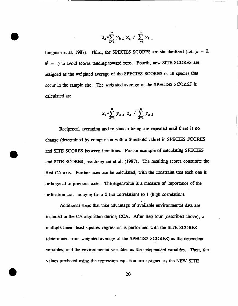
Jongman et al. 1987). Third, the SPECIES SCORES are s t a n w e d (i.e. p = 0,

62 = 1) to avoid scores tending toward zero. Fourth, new SITE SCORES are

assigned as the weighted average of the SPECIES SCORES of all species that

occur in the sample site. The weighted average of the SPECIES SCORES is

calculated as:

Reciprocal avemging and r e - s t a a s g are repeated until there is no

change (deteimined by comparison with a threshold value) in SPECIES SCORES

and SITE SCORES between iterations. For an example of calculating SPECIES

and SITE SCORES, see Jongman et al. (1987). The resulting scores constitute the

first CA axis. Further axes can be calculated, with the constraint that each one is

orthogonal to previous axes. The eigenvalue is a measure of importance of the

ordination axis, ranging from 0 (no correlation) to 1 (high correlation).

Additional steps that take advantage of available environmental data are

included in the CA algorithm during CCA. After step four (described above), a

multiple linear least-squares regression is performed with the SlTE SCORES

(determined from weighted average of the SPECIES SCORES) as the dependent . .

variables, and the environmental variables as the independent variables. Then, the

values predicted using the regression equation are assigned as the NEW SITE

SCORES. These NEW SITE SCORES are linear combinations of the

environmental variables. The NEW SITE SCORES are then used in subsequent

itexations of the algorithm.

The NEW SITE SCORES produced by CCA are used to plot an ordination

diagram that allows visualization of the species/environment relationships (Figure

3). Environmental variables are represented by lines of lengths proportional to

their importance, and direction indicative of comiations between variables. The

position of a species along a gradient is determined by drawing a perpendicular

line from the species point to the gradient line (Figure 3.) To evaluate an axis

quantitatively, its eigenvalue is used. The eigenvalue measures how much

variation in the species data is explained by the axis, and therefore, by the

environmental variables. I used the eigenvalues from analyses using various

combinations of the data sets to compare models that explain the variation in the

species abundance data.

I used methods proposed by B o d et al. (1992) to partition the habitat,

landscape, and spatial components of the variation in the species data. I compared . .

different models in CCA using the habitat, landscape, and location coordinate

variables (Table 7). The resulting sum of all canohical eigenvalues was used to

calculate the proportion of variabiiity explained relative to the total variation in the

bird species matrix.

To describe spatial structure in the data, I &rived a location coordinate

matrix using steps described by Legendre (1990). This matrix, 2, included the

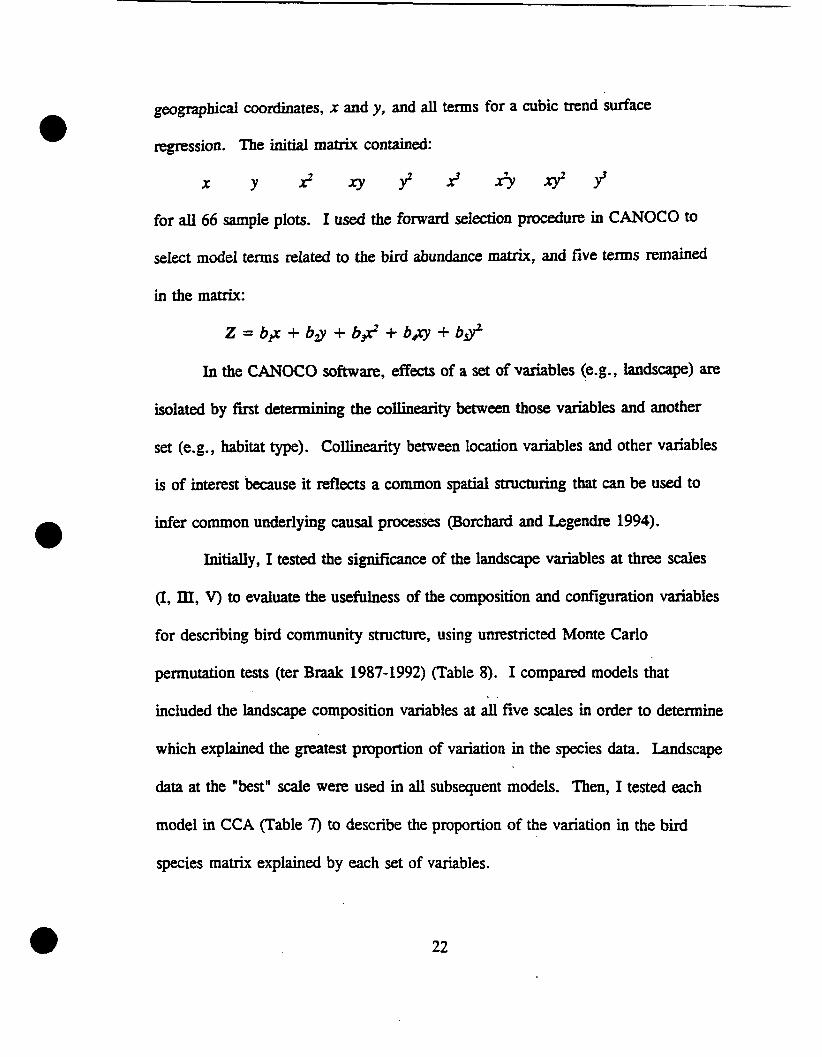
geugraphical coordinates, x and y, and all terms for a cubic trend surface

regression. The initial matrix contained:

x Y *3 xy J i f i X J y l

for a l l 66 sample plots. I used the fornard selection procedure in CANOCO to

select model terms related to the bird abundance &, and five terns remained

in the matrix:

Z = b $ + b g + b $ + b m + b $

In the CANOCO software, effects of a set of variables (e.g., landscape) are

isolated by first determining the coIlinearity between those variables and another

set (e.g., habitat type). Collinearity between location variables and other variabIes

is of interest because it reflects a common spatial structuring that can be used to

infer common underlying causal processes (Borchard and Legendre 1994).

Initially, I tested the si@cance of the landscape variables at three scales

(I, III, V) to evaluate the usefulness of the composition and configuration variables

for describing bird community structure, using unrestricted Monte Carlo

permutation tests (ter Braak 1987-1992) (Table 8). 1 compared models that

included the landscape composition variables at all five scales in order to determine

which explained the greatest proportion of variation in the species data. Landscape

data at the "best" scale were used in all subsequent models. Then, I tested each

model in CCA (Table 7) to describe the proportion of the variation in the bird

species matrix explained by each set of variables.

Chapter IZI

Results

cape Pattern Description

The landscape context of the sample plots was dominated by the extensive

background matrix of native and introduced grasslands (Figure 4). The m i d m

tsllgrass, and hsy/pastwe mver types dominated all other cow types at all five scales

Figure 5). The shee of the anaiysis profoundly influenced the d d p t i o n of

landscape. The mean percent of each analysis window claySed as urban g raddy

increased as window size increased (Figure 6). The distriiution of urban cover types at

scale V was similar to scale IV, but the mean percentage at scale V was higher than

that at scale N due to several outliers in the scale V data Urban composition did not

influence landscape analyses at scale I because of its limited distribution. In general,

the mean percent of grassland cover trpes decreased as mean percent of urban cover

types increased in the landscape.

The change in variance, or distribution of variables, between scales reflected the

shift in dominance away fiom grassland types toward urban types in the landscape.

The largest change in variance between scales occ&;d between scales I and I1 for the

following variables: percent urban, perimeterlarea ratio, percent tallgrass, contagion,

and dlfd (double log fractal dimension) (Figure 7). The largest change in variance for

number of patches, however, occurred at scale V.

Habitat Preference

Some bud species showed a preference for certain habitat types at the scale of

the sample plot. Based on number of occurrences in each habitat type, the Savannah

Sparrow and the Bobolink preferred tallgrass and hayfield habitats (Table 9). The

Homed Lark and the Lark Sparrow were only observed in upland habitats (shortgrass

or mixed grass). Red-winged Blackbird, Robin, and Common Grackle were more

common in lowland plots. The Grasshopper Sparrow and Vesper Sparrow were more

often sighted in upland plots. Species with no apparent preference based on the raw

count data included Western Meadowlark, European Starling, House Finch, and House

Sparrow.

In a few cases, species that preferred the same habitat type exhibited differences

in spatial distribution among the plots (Figure 8). Homed Lark and Lark Sparrow

occurred in similar upland habitats, but never occurred together at the same plot.

Furthermore, a majority of plots where the Homed Lark occurred were in the

expansive mixed and shortgrass areas in the south, whereas the Lark Sparrow was only

observed in the block of mixed and shortgrass north of the city of Boulder. The . .

distribution of Savannah Sparrows and Bobolinks overlapped at tallgrass and hayfield

plots.

Importance of Ludcape Context . .

Grassland-nesting bird species generally preferred areas with a less urbanized

landscape. Scatter plots of bud abundance for individual grssrland spede~ and urban

context (percent of combined urban cover types) at scales I1 through V exhibited

similar patterns, with a large amount of variation in abundance at low levels of urban

context (Figure 9.). High levels of bird abundance rarely occmed at higher levels of

urban landscape composition. Pearson's correlation coefficient indicated significant

negative correlations (p < 0.05) between Meadowlark, Grasshopper Sparrow, and

Vesper Sparrow abundance and urban context at scale IIL Among the individual

species analyzed using logistic regression, only the Grasshopper Sparrow showed a

significant negative relationship with urban landscape context (Table 10).

The negative relationship between grassland bird abundance and urbanization

was influenced by spatial structure. Ordinary least squares regression analysis showed

significant negative relationships between grassland bid abundance, when abundance

values for the eight species were combined, aid percent urban composition at scales XI,

III, N, and V. AICC statistics varied fiom 276.636 (scale IlJ to 267.071 1 (scale V).

The differences in AICC values were not great enough to select a "best" model. The

residuals &om the scale V regression contained spatial autocorrefation (Moran's I =

0.175, p < 0.001). The coefficient &om spatial autckegrrrdon was correspondingly

high (lambda = 0.7983).

Suburban-nesting bird species were more common on sample plots within a

more urbanized landscape. The European Starliig and House Sparrow had sigr&cant

positive relationships with urban composition at scales 11, III, IV and IV (Pearson's

correlation coefficient p < 0.05). Results of regression analysis confhed correlation

of suburban nesters with urban composition at scales &.IlI, IV, and V. The "best"

model included urban data at scale Ill (AICC = 281.3844). AICC values did not differ

greatly, but I used the data at scale Ill to evaluate the spatial autocorrelation, which

was significant (Moran's I = 0.144, p < 0.001). The si@cance of the spatial effects

were reff ected in the high value of lambda (0.71 52). Using logistic regression, a

significant positive relationship was identified between the House Sparrow and urban

context.

Grassland bird species associated with certain habitat types at the plot level

were more abundant in landscapes with higher percent composition of their preferred

grassland types. Maximum levels of abundance for the Lark Sparrow and Homed Lark

were only observed at the highest levels of upland grassland type composition (sum of

midgrasdmixed grass and midgrass/shortgrass) (Frgure 10). Scatterplots of Savannah

Sparrow and Bobolink abundance against lowland grassland landscape composition

measures (sum of tallgrass and haylpasture types) exhibited similar patterns. There was

a significant positive relationship bemeen these species' abundance and grassland

composition variables at scafe ID in tests of ~eano~r '~orreiat ion Coefficient @ <

0.05). 4

Bird Community Patterns in Relation to M c a p e Stnrcture

Avian community structure was strongly influenced by landscape context. The

ordination diagrams confinned the impo-ce of landscape context to grassland and

suburban species M the thne scales analyzed in CCA (Figure 1 la - 1 lc.). Species

associated with landsapes dominated by upland grasses and those species associated

with lowland tallgrass or hayfield landscapes were grouped dong these gradients.

Quadrant locations of particular grassland species rdected their a f h i t y for landscape

context of a particular grassland type. For example, the Bobolink, Savannah Sparrow,

and Red-winged Blackbird were all located at the high end of the tailgrass and wetland

gradients in the ordination diagrams. The first axis (horizontal) was highly correlated

with percent mixed grass and percent shortgrass cover types at all tbree scales and the

eigenvalue of this axis indicated a strong gradient (Figure 1 1 a - 1 1 c.).

The pefcent of urban cover types in the landscape was not as important as the

percent of grassland types in determining bud community structure. The second axis

(vertical) was correlated with percent urban cover types at scales III and Y, but this

axis had a low eigenvalue (< 0.3), indicating a weak gradient (ter Braak and

Verdonschot 1995). At scales EX and V, the suburban species were grouped at the

high end of the urban gradient, and the grassland species f d at the lower end of this 9 .

gradient. The Bobolii was an exception, and fell at the midpoint of the urban

gradient.

The variation in the species community data explained by the landscape data

increased with scale (Figures 1 1 a. - 1 1 c.). At scale I, 34.99% of the variation was

accounted for by the set of independent variables. Two, of the landscape configuration

indices were significant to the ordination at this scale (Table 8). Fractal dimension and

perimeterlarea ratio were non-sigificant for scales I, Dl, and V. At scale III, more of

the predictive power was contained in the independent miables (39.73% explained

variation). One of the landscape indices (contagion) was significant at this scale, and

the composition variables differed somewhat fiom those! included at scale I. At scale

V, 45.90% of the variation was explained by the landscape variables (n = 66). Six of

the composition variables were significant to the ordination at scale V, but none of the

configuration indices were significant. Because the wuiables at scale V explained the

greatest amount of variation, these variables were used in h the r analysis of landscape

influence on the bid species.

Bird Community Patterns in Relation to Habitat Type

Habitat type played a role in d e t e n - g bid community structure. However,

landscape context had an even greater influence on avian patterns. Analysis of habitat

effects using CCA explained roughly 26.43% of the variation in the bid data (Table

11). I compared this analysis with the results using landscape data (cover type

composition only) fiom scale V. The landscape data'explained a higher percentage of

the variation than the habitat type data (46.20%). There was a substantial amount of

collinearity in the landscape and habitat data, however, as 17.70% of the variability

explained by landscape could also be explained by habitat type (Table 12).

l h Irnpnkzna of Location

The structure of the avian community was influenced by geographic location

A common spatial structuring existed between the landsape and habitat variables,

indicated by a fXr amount of coilin- between the landscape and habitat variables

and the geographic coordinate matrix (Table 12). Some variation in the bird species

data was explained by the location matrix (12.98%). but could not be dated to the

landscapehabitat variables A sub- amount of variation was unexplained after

habitat, landscape, and location were taken into account. This indicated that other,

unmeasured fktors, were influencing the bird comrmrnity structure.

Chapter IV

Discussion

Interrelationships: Lmdscape Scale and Bird Communi~ Pattern

Influences on the bird species community in the Boulder Open Space were

apparent at Merent spatial scales. At the scale of the sample plot, habitat preferences

played a role in determining bird community structure. However, these patterns were

not as clear and definitive as the patterns of distribution related to landscape context.

The extensive grassland mosaic captured in measurements at the &ha scale were

interrupted by patterns of urban encroachment at the 4Gha scale.

The area between 6 and 40 ha is the geographic scale at which processes and

patterns associated with urbanization were evident, both in terms of bird community

and landscape characteristics. Landscape patterns at this scale reflect two components

of change; an increase in area of urban cover types and a decrease in area of grassland

cover types. Detectible change in landscape pattern at these scales may be related to

the location of the bird sample plots, many of which were positioned at the edge of a

suburban development.

The scale-dependent patterns were most closely related to the area of grassland

cover types. The results of the ordination analyses indicate that the patterns of

grassland habitat in the landscape were more important than the amount of urban

habitat in structuring the bird community. Urban landscape composition was a

significant variable in the ordination analysis. However, a weak gradient was indicated

by the axis associated with this variable. Composition of grasJland typ& apkially

midgrass and shortgrass types, had a stronger role in det&g bird community

patterns. A common characteristic of fragmentation is the loss of area in certain habitat

types, and its subsequent replacement by some other type, or land use (Andren 1994).

This change in habitat composition o m e d in the Boulder study area, where the mean

of the grassiand habitat types decreased as the mean of the urban cover types increased

in the landscape. Based on the results of my study, I hypothesize that the more

important component of change is the decrease in grassland cover types, rather than the

increase in urban types. It may be possible to test this hypothesis if study areas could

be identified where grassIand habitats were being replaced by non-urban cover types.

The rehionship between urban landscape context and individual grassIand bird

species abundance suggested by the scatterplots (Figure 9) was not confixmed by the

ordination results, perhaps because there were fewer suburban nesters included in the

analysis. Ordination provided a description of the bird community in relation to

landscape gradients using species abundances at the sample sites where they were

observed to weight the ordination. The relatively greater importance of the grassland . .

gradients compared to the urban gradient may have resulted from inclusion of fewer

suburban nesting species.

The importance of landscape context in explaining bird community structure

was also noted in other studies. Pearson (1 993) reported similar results in his study of

wintering birds in the Georgia piedmont, where 3.0-90 % of the variation in bird

abundance and divenity was accounted for by landscape variables. &ght and Moms

(1996) emphasize the importance of examinbg the effects of habitat selection before

assessing the role of landscape composition and mucrun. In my study, as well as

Pearson's (1993), habitat type was also an impoxtaut component of the &on. The

results of this study indicate that much of the effect of habitat type can be also be

predicted by landscape context.

The Importance of Location

Geographic location explained some of the variation in bird distribution and

abundance. Locational analysis identified a common spatial structure between bid

community and landscape pattern. Spatial structure reflects the non-uniform and non-

random manner in which biological and environmental components of nature are

distributed (Legendre 1993). The action of physical processes structuring the

arrangement of these components is visible in either gradients or patchiness on the

landscape.

The effects of geomorphology, hydrology, and land use on landscape patterns . .

are visible in the land-cover maps (Figures 4 and 12). A geomorphologicai shift occurs

at the mountain-plains boundaq. To the east of this boundary, the extensive

background grassland matrix is patterned by the hydrology of Boulder Creek, and land

use practices driven by economy, politics and culture. The fixtors determining land use

are intertwined, but the results of these forces are evident in Qrating regimes (reflected

in pattern of midgrass and shortgrass cover types), extent of *cultural areas, and the

preservation of grassland habitatsin Open Space properties (delineated in Figure 1).

Additional spatial structuring in communities may resuit &om biotic interactions

such as predation, competition, reproduction, and death. Spatial structuring in the

Boulder bird community may be linked to biotic interactions resulting &om

urban/grassland landscape patterns. The mosaic of cover types in the urbanized . .

landscape may provide opportunities for M o n by species not adapted to grasslands,

such as the urban nesters observed in this study. Uninterrupted expanses of grassland

habitat contain few patches of different cover types that may serve as refirgia for

species not adapted to the variations in cfimate and resources present in grassland

habitats (Wiens 1974). Patches of urban vegetation may allow non-grassland species,

such as European Starlings, American Robins, House Sparrows, House Fiches and

Common Grackles, to exploit grassland resources when climate and productivity are

favorable. Increased opportunities for utilization of grassland resources by non-

grassland species may lead to interspecific competition for resources.

Biogeography and Urbanization

Biogeographical boundaries reflecting changes in bird abundance patterns in the

Great Plains are likely related to climate (Bock et al. 1977). A predominant gradient in

moisture regimes probably influences bird abundance patterns indirectly through its

effects on vegetation patterns. Urbanization can override the effects of climate,

moderating the mremes of climate at local and is a p o w d dioeubance in

itselt(Jokimaki and Suhonen 1993). Studies in Finland demonstrate the effects of

urbanization on species composition and diversity. Based on their biogeographical

analysis, the effects of latitude are apparently tempered by the urban environment. An

interesting question for fbture study would be: How are micro- and macmclimatic

effects of urbanization changing the distriiution of species in Front Range grassland

communities?

The need to integrate ecological and biogeographical principles has been

emphasized (Bock 1987). At a regionai scale, the dimension of geographic variation in

abundance adds important information to maps of species distniution The observed

local distributions in the Lark Sparrow and the Homed Lark demonstrate such

geographic variation. The geographic range of these species coincides regionally, but

effects of either abiotic (e.g., climate) or biotic (e.g., interspecific competition)

variables at the local scale prevail over broader-scale influences (Wiens 1989b). It was

hypothesized that locd habitat features, such as shale soils, influenced the Lark

Spanow's distribution (C.E. Bock, pers. comm.). This soil type occurs mainly in the. . .

areas where Lark Sparrows were obsewed. An alternate hypothesis was that the

presence of one species precludes that of the other, because of biotic interactions (e.g.,

competition). The Savannah Spamow and Bobolink occurred only in tallgrass or

hayiield plots, but their distribution among these plots overlapped. Habitat type

descriptions at finer scales may be needed to interpret overiapping distributions.

Common vs Rare Species

The results of this study relate to the importance of comparing common and

rare sped= disarued by Bock (1987). Wide geographic distriiution and high

abundance are o h correlated, implying that common species share arrlogic.1

characteristics that differ &om those of rare species. In my study, I compared a group

of "oomrnon" species (suburban nesters) with "rare? species (gadand nesters). The

Wring ecological properties of common and rare species emerged along the gradients

of landscape pattern What proasses are involved in creating the obrerved patterns

among common and rare species in my study? Does predation of gmund-nesting

grassland bids by domestic animals influence their distriiution in urbanized

landscapes? Do these two groups of species respond differently to environmental

effects of urbanization, such as noise levels and levels of human activity?

Other Comnn&rm'ons

Data Sources and Clasn~cation Scheme

Description of landscape pattern at any scale is directly related to the data . .

source used to aeate the map. The resolution of the data source in this study was

determined by the spatial extent of the area to be mapped, and the classification scheme

was chosen to relate to boundaries considered important to species of interest. In using

mapped data, it is important to recognize maps as models; an alternative form of

looking at reality that incorporates cartographical conventions of generalization, feature

displaamat and symbolization and Thompson 1992). The result of modeling

the landscape in this fashion is likely to have a strong element of human prception.

The classification scheme I used was f M y detailed. SuccessfU descriptions of

habitat relationships depend on identification of habitat types that species of interest

recognize (Knight and Monis 1996). In Knight and Morris1 study of small mammal

species, the large number of habitat classes identified with sateUite imagery were

excessive in describing the three types of habitat found to be important to habitat

selection. It is possible that this may be the case in my dysis , and a simplified

classification of landscape cover types could provide adequate, or better, results. It is

also worth considering that more detailed categories of plot-level habitat types would

provide a fairer analysis for comparison of the importance of habitat versus landscape

components of variation. In my study, the importance of landscap may have been

more evident because I used more detail in landscape description, including five scales

of analysis. The distribution of the Homed Lark and Lark Sparrow indicated the

possible importance of h e r scale habitat information (e.g, soil type). The addition of

detail in the habitat categories could increase the detection of their role in determining , .

bird distribution and abundance.

Description of Lumkcape Pattern

There is a spectrum of spatial pattern created by disturbance. Fragmentation

has been emphasized (e.g. Herkert 1994), but other descriptions may be better suited to

grasslands in general, and to the Boulder landscape in particular. ~dedtification of

u d landscape merriu nkds fimher research. Patterns created by urbanization might

be best described by metrics that capture "sbrinkage" or "attrition" (Forman 1995), or

"indentation" (Zipperer 1993). A limitation of fragmentation metrics may be their

development in computer simulations that have no link to ecological phenomena (e-g.

O'NeiI1 et d. 1988, Turner et d. 1989). A metric that best describes patterns of

importance reasonably needs to be derived for a specific research question and a

particular study area. This was the approach taken by Shumaker (1996), who

developed a pattern index that was consistent with predictions for dispersal success.

Scale

Considering scale as a primary focus of research efforts has been advocated by

Wiens (1989b). Obsewations f?om this study provide insights toward that direction. A

common issue in research whose purpose is to relate biological processes (e.g.

distribution, abundance, reproductive success, dispersion) to landscape patterns at

multiple scales is the spatial. arrangement of sample sites. Using GIs, sampling of s .

landscape pattern is only limited by the map extent, but observations of biological

processes are restricted by a number of factors. In some cases, sampling is determined

by the location of nest sites (e-g. Baker et al. 1995). A very common situation is the

need to sample within political boundaries, especially on publicly owned lands.

The location of the bird sample plots for the Boulder study affected the

landscape pattern description, and the ability to detect heterogeneity at multiple d e ~ .

The averaging of effects of local heterogeneity at broader scales (l%ens 1989b) is

altered when sample sites are close together relative to scales of interest. As the size of

the window increases, more and more overlap oca;us between windows, and spatial

correlation becomes spatial identity where sample plots occur in dusters. In essence,

66 landscapes are reduced to a smaller number of grouped landscapes (Figure 13).

This overiap in landscape pattern data could be the cause of the increased

amount of variability explained at larger area scales using CCA Rather than a simple

averaging effect, increased explanatory power may have resulted because more samples

had similar values. In tenns of identification of changes in heterogeneity, however, no

scale thresholds were identified beyond the two smallest areas. The windows at these

scales had the least amount of overlap.

Conclusion

Some implications for bird conservation in grasslands near Boulder, Colorado,

and for hture investigations of biid distribution and abundance in relation to habitat . .

and landscape characteristics can be made based on observed patterns. The

significance of grassland cover type composition in the landscape in relation to biid

abundance and distribution would indicate the need ro conserve large areas of grassland

habitat. However, observed patterns in bird abundance in relation to urban landscape

context indicate grassland birds occur more abundantly at low levels of an uhan

gradient. In addition, two hypothesis related to biotic factors are linked to the

assumption that urban cover types are a critical component of c o d t y m u d n g .

First, the idea that competition with suburban nesting species may influence the

distribution of grassland nesting species leaves open the possiiity that urban cover

types provide opportunities for this interspecific competition that would not otherwise

exist. Second, the hypothesis that predation by domestic animals &scts bird

abundance and distribution in grasslands is predicated on the interspersion of urban and

grassland cover types.

Further investigations are needed to confirm and clarifjl these observations.

The unequal number of grassland bird species compared to suburban nesting birds may

have led to under-emphasis of the importance of urban co%r types in determining

distribution of bird species in Boulder area grasslands. A study designed to isolate the

effects of grassland habitat loss would provide insight into the relative importance of

shifts in grassland/urban area Furthennore, additional detail in plot-level habitat type

descriptions could provide a fairer comparison between landscape and habitat effects in

structuring the bird community.

Litexaturn Cited

Abler, R.F. 1987. What shall we say? to whom shall we speak? Presidential

Address. Annals of the Association of American Geographers

77(4):511-524.

Andren, H. 1994. Effects of Mitat fragmentation on birds and mammals in

landscapes with different proportions of suitable habitat: a review. Oikos

71 ~355-366.

Andrewartha, H.G. and L.C. Birch. 1954. The distribution and abundance of

animals. Chicago: University of Chicago Press.

Andrewartha, H.G. and L.C. Birch. 1984. The ecological web. More on the

distribution and abundance of animals. Chicago: University of Chicago

Press.

Baker, B. W., B.S. Cade, W.L. Mangus and J.L. McMillen. 1995. Spatial

analysis of Sandhill Crane nesting habitat. Journal of Wildlife Management

59(4):752-758.

Bennett, B.C., C.E. Bock and J.H. Bock. 1997. Biodiversity of Open Space

Grasslands at a suburban/ag~icultud interface. Part I. Vegetation. Final

Report, August 11, 1997.

Blair, RB. 1996. Land use and avian species diversity along an urban gradient.

Ecological Applications 6(2) 506-5 19.

Bock, C.E. 1987. Distribution-abundance relationships of some Arizona landbirds:

A matter of scale? Ecology 68(1): 124-129.

Bock, C.E. 1997. The role of ornithology in consemation of the American West.

Condor 99(1): 1-6.

Bock, C.E. 1998. Professor of Biology, University of Colorado, Boulder.

Personal Communication.

Bock, C.E. and J.H. Bock. 1995. Biodiversity of Boulder Open Space grasslands

at a suburbanlagricultural interface. Preliminary results and

recommendations based on work complet& in 1994. Unpublished report.

Bock, C.E., J.H. Bock, and B.C. Bennett. In press. Songbird abundance in

grasslands at a suburban interface on the Colorado . . High Plains. Studies in

Avian Biology.

Bock, C.E., J.H. Bock and L.W. kpthien. 1977. Abundance pktem of some 1 bird species wintering on the Great Plains of the U.S.A. Journal of

Biogeography 4: 101-1 10.

Borcard, D. and P. Legendre. 1994. Environmental control and spatial structure

in ecological communities: an example using oribatid mites (Ad,

Oribatei) . Environmental and Ecological Statistics 1 : 37-6 1. 1

Borcard, D, P. Legendre and P. Dqeau. 1992. Partialling out the spatial I

component of ecological variation. Ecology 73(3): 1045- 1055. 1

Bragg, T.B. and A.A. Steuter. 1996. Prairie ecology - The mixed prairie.

Chapter 4 in Samson, F.B. and F.L. Knopf, eds. Prairie Conservation:

Preserving North America's Most Endangered Ecosystem. Island Press.

Cliff, A.D. and J.K. Ord. 1973. Spatial autoconelation. Methuen, Inc. NY . <

178p.

Cornell, J.H. 1983. On the prevalence and relative importance of interspecific

competition: evidence from experiments. American Naturalist 122: 66 1-697.

Cressie, N. 1991. Statistics for spatial data. John Wiley and Sons, Inc. 900p.

Czap1ewsld7 R. 1994. Variation approximations for assessments of ~ l a s s ~ c a t i ~ n

accuracy. USDA Forest Service Research Paper RM-3 16. 29 p.

Dillwoxth, M.E., J.L. whistler, and J. W. Merchant. 1994. Measuring landscape

structure using geographic and geometric windows. Photogrammetric

Engineering and Remote Sensing 60(10): 1215-1224.

ERDAS 1997. Imagine User's Guide: Online Help.

ESRI 1996. Arc/Info and Arc/Grid, version 7.0. I. Environmental Systems

~eseakh Institute, Redlands, California.

Forman, R.T.T. 1995. Land mosaics: The ecology of landscapes and regions.

Cambridge University Press, Cambridge.

Gleason, H.A. 1926. The individualistic concept of the plant association. Bulletin . .

of the Tomy Botanical Club 53:l-20.

Greig-Smith, P. 1952. The use of random and continuous quadrats in the study of

the structure of plant communities. Annals of Botany New Series

16:293-316.

Herken, J.R. 1994. The eff- of habitat fragmentation on midwestern grassland

bird communities. Ecological Applicatiolls 43461-471.

Horne, J.K. and D.C. Schneider. 1995. Spatial variance in ecology. Oikos

74: 18-26.

Jensen, J.R. 1986. Introductory digitat image pmssing: A m o t e sensing

perspective. Prentice-Hall, New Jersey.

Jokimaki, J. and J.Suhonen. 1993. Effects of urbanization on the breeding bird

species richness in Finland: a biogeographical comparison. Ornis Fenuica

70~71-77.

Jongrnan, R.H.G., C.J.F. ter Braak and O.F.R. van Tongeren, eds. 1987. Ilata

analysis in community and landscape ecology. Pudoc Wageningen,

Netherlands. 29%. . .

Knight, T.W. and D.W. Morris. 1996. How may habitats do landscapes contain?

Ecology 77(6): 1756- 1764.

Knopf, F.L. 1996. h i r i e LRgacies -Birds. Chapter 10 in Samson, F.B. and

F.L. Knopf, eds. Prairie Conservation: Preserving North America's Most

Endangered Ecosystem. Island Press.

Kotliar, N.B. 1996. Scale dependency and the expression of hierarchical structure

in Delphinium patches. Vegetatio 127: 1 17-128.

Laurini, R. and D. Thompson. 1992. Fundamentals of spatial information

systems. The A.P.I.C. Series, No. 37. Academic Press.

hgendre, P. 1990. Quantitative methods and biogeographic analysis. Pages 9-34

in D.J. Garbary and R.R. South, editors. Evolutionary biogeography of the

marine algae of the North Atlantic. NATO MI Series, Volume G 22.

a Springer-Verlag, Berlin, Germany.

Legendre, P. 1993. Spatial autoco~~elation: Trouble or new paradigm? Ecology

74(6): 1659-1673.

Legendre, P. and M.-J. Fortin 1989. Spatial pattern and ecological analysis.

Vegetatio 80: 107- 13 8.

Li, H. and J.F. Reynolds. 1995. On definition and qetif~cation of heterogeneity.

Oikos 73(2):280-284.

Long, M.E. 1997. Colorado's Front Range. National Geogxaphic 190(5): 80- 103.

McGarigal, K. and W.C. McComb. 1995. Relationships W e e n landscap

structure and breeding birds in the Oregon coast range. Ecological

Monographs 65(3):235-260.

McGarigal, K., and B.J. Marks. 1995. FRAGSTAn: Spatial pattern analysis

program for quantifyiig landscape structure. General Technical Report

PNW-GTR-531. Portland, OR: U.S. Department of Agriculture, Forest

Service, Pacific Northwest Research Station. 122 p.

McIntosh, R.P. 1985. The background of ecology: concept and theory.

Cambridge University Press, Cambridge.

Meetenmeyer, V. 1989. Geographical perspectives of space, time, and scale.

Landscape Ecology 3(3/4): 163- 173.

Mutel, C.F. and J.C. Emerick 1992. From grassland to glacier. The natural

history of Colorado and the surrounding region. Johnson Books, Boulder,

Colorado. 285 p.

Neter, J., M.H. Kutner, C.J. Nachtsheim and W. Wasserman, eds. 1996. Applied

46

linear statistical models. Fourth Edition. Irwin Publishers. 1408p.

Oksanen, J. and P.R. Minchin. 1997. Instability of ordination results under

changes in input data order explmatibns and remedies. Journal of

Vegetation Science 8:447-454.

O'Neill, RV., D.L. DeAngelis, J.B. Waide and T.F.H. Allen. 1986. A

hierarchical concept of ecosystem. Princeton University Press, Princeton,

N. J.

O'Neill, R.V., J.R. Krummel, RH. Gardner, G. Sugihara, B.Jackson, D.L.

DeAngelis, B.T. W e , M.G. 'Turner, B. Zygmunt, S.W. Christensen,

V.H. Dale, and R.L. Graham. 1988. Indices of landscape pattern.

Landscape Ecology 1 : 153-162.

Palmer, M.W. 1993. Putting things in even better order: The advantages of . .

canonical conespondence analysis. Ecology 74(8) : 22 15-2230.

Pearson, S.M. 1993. The spatial extent and relative influence of landscape-level

factors on wintering bird popularions. Landscape Ecology 8(1): 3- 18.

Pearson, S .M., M.G. Turner, RH. Gardner, and R.V. O'Neill. 1996. An

47

organism-based perspective of habitat fragmentation. Chapter 6 in

Biodiversity in Managed Landxapes. Oxford UniveniQ Press, New York,

Oxford.

Quinn, J.F., and A.E. Dunham. 1983. On hypothesis testing in ecology and

evolution. American Naturalist 122602-617.

Reynolds, R.T., J.M. Scott, and N. A. Nussbaurn. 1980. A variable circular-plot

method for estimating bird numbers. Condor 82:309-313.

Ricklefs, R.E. 1975. Competition and the structure of bird communities [review].

Evolution 29:581-585.

Samson, F.B. and F.L. Knopf. 1994. Prairie conservation in North America.

Bioscience 44: 41 8-42 1.

Shumaker, N.H. 1996. Using landscape indices to predict habitat connectivity.

Ecology 77(4): 1210-1225.

Sodhi, N.S. 1992. Comparison between urban and rural bird communities in

prairie Saskatchewan: Urbanization and short-term population trends.

Canadian Field-Naturalist 106(2):2 10-215.

StatSci, 1995. Splus, statktical soffwan. Mathsoft, Seattle, Washington

Steinauer, E.M. and S.L. Collins. 1996. Prairie ecology - The tallgrass prairie.

Chapter 3 in Samson, F.B. and F.L. Knopf, eds. Prairie Conservation:

Preserving North America's Most Endangered Ecosystem. Island Press.

ter Braak, C.J.F. 1985. Correspondence analysis of incidence and abundance data:

properties in terms of a unimodal response model. Biometxics 41:859-873.

ter Braak, C.J.F. 1986. Canonical correspondence analysis: a new eigenvector

technique for multivariate direct gradient analysis. Ecology 67: 1 167-1 179.

ter Braak, C.J.F. 1987. The analysis of vegetation-environment relationships by

canonical conespondence analysis. Vegetatio 69: 69-77.

ter Braak, C.J.F. 1987-1992. CANOCO: a FORTRAN program for canonical

community ordination. Microcomputer Power, Ithaca, New York, USA.

ter Braak, C.J.F. and P A M . Verdonschot. 1995. Canonical correspondence

analysis and related multivariate methods in aquatic . . ecology. Aquatic

Sciences 57(3):255-289.

Turner, M.G., R Costanza and F.H. Skiar. 1989. Methods m evaluate the

performance of spatiaf simulation models. Ecological Modelling 48: 1-18.

Whittaker, R.H., ed. 1973. Ordination and classification of communities. Junk,

The Hague.

Wiens, J.A. 1974. Climatic instability and the "ecological saturation" of bird

communities in North American grasslands. Condor 76:385-400.

Wiens, J.A. 1989a. The ecology of bird communities. Vol. 2. Processes and

variations. Cambridge University Press.

Wiens, J.A. 1989b. Spatial scaling in ecology. Functional Ecology 3:385-397.

Wiens, J.A. 1990. On the use of 'grain' and 'grain size' in ecology. Functional

Ecology 4720.

Wiens, J.A. 1995. Landscape mosaics and ecological theory. Chapter 1 in

Mosaic Landscapes and Ecological Processes. Hansson, L., L. Fahrig, and

G. Merriam, eds. Chapman and Hall, London.

Zipperer, W. C. 1993. Deforestation pattern and their effects on .f orest patches.

Landscape Ecology 8: 177-1 84.

Zipperer, W.C. and R.V. Pouyat. 1995. Urban and suburban woodlands: A

changing forest system. The Public Garden lO(3): 18-20.

Table 1. Grassland and suburban nesting bird species observed in the Boulder Open Space sample plots.

Common name Scientific name Grassland (G)/ Suburban (S)

Savannah sparrow Passerculus sandwichensis G

Western meadow lark

Bobolink

Gmshopper sparrow

Homed lark Eremophila @esnis

Vesper sparrow

Lark s p m w

Red-winged blackbird

American Robin

European starling

Common grackle

House finch

House sparrow

-O&CUS m ' c m r r ~ S . .

Passer domesricrrs S

Table 2. Earth sulface chacteristics detected by the Thematic Mapper S p d Bands.

Region of the Electromagnetic Spectrum Rdectance Prop* (measured in micrometers)

Band 1: 0.45-0.52

Band 2: 0.52-0.60

Band 3: 0.63-0.69

Band 4: 0.76-0.90

Band 5: 1.55-1.75

Band 6: 10.4-12.5

Band 7: 2.08-2.35

Penetration of water bodies

Green ~flectance of healthy vegetation

Red chlorophyll absorption, vegetation

Vegetation biomass

Turgidity of plants; clouds, snow, ice

TemperatuIle

Geologic formations

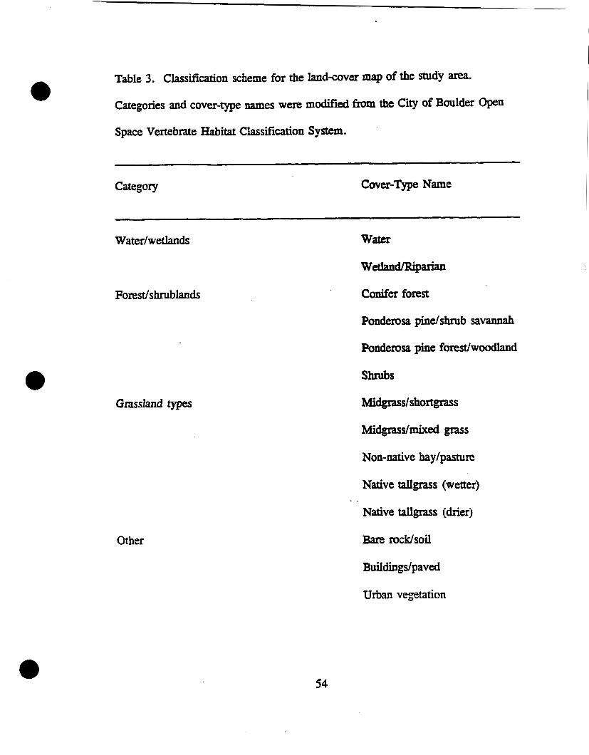
Table 3. CIassification scheme for the landcover map of the studjr area.

Categories and cover-type names were modified from the City of Boulder Open

Space Vextebrate Habitat Classification System.

Category Cover-Type Name

--

Water/wetlands Water

WerlandlRiparian

Forest/shrublands Conifer forest

Pondemsa pine/shrub savannah

Pondemsa pine forest/woodland

Shrubs

Midgrasslshortgrass

Midgrassfmixed grass

Non-native haylpasture

Grassland types

Native tallgrass (wetter) . .

Native tallgrass (drier)

Other Bare rock/soil

Urban vegetation

Table 4a. Error matrix and kappa statistics used for map accuracy assessment. Row and column numbers correspond to cover types listed, below. Rows are data from random points (n=86), columns are data from the l a ~ ~ d cover map. No individual accuracy assessment was possible for 5.wetlandlriparian (no samples). - - -

Error Matrix

Kappa Statistics

Overall accuracy 0.5 Overall Kappa 0.426

Table 4a. Continued.

Cover type number and name Individual Kappa Statistics

1 . Water 1.00000000 2. Conifer 1.00000000 3. Ponderosa pinelshmb savannah 0.585542 17 4. Midgrass/mixed grass 0.1 1794872 5. Wetlandlriparian no samples 6. Midgrass/shortgrass 0.23555556 7. Non-native haylpasture 0.24561 404 8. Ponderosa pine forestlwoodland 0.241 17647 9. Shrubs 0.80888889 10. Bare rocWsoil 0.54497354 I I . Buildingslpaved 0.63682432 12. Urban vegetation 0.48809524 13. Native tallgrass (wetter) -0.02380952 14. Native tallgrass 0.00000000

Table 4c. Kappa statistics using combined cover types (midgrass types, tallgrass types, urban types and conifer types).

Error Matrix

c, Overall accuracy 0.6395 00 Overall Kappa 0.553

Cover type name and number: Individual Kappa Statistics

1 . Water : 1.0000000 2. Conifer types 0.7766234 6. Midgrass types 0.3892045 7. Non- native hay/pasture 0.2456140 10. Bare rocWsoil 0.8088889 12. Urban types 0.6748582 14. Tallgrass types 0.6504065

Table 4d. Kappa statistics using combined cover types (midgrass and hayfield types, tallgrass types, urban types and conifer types). - -

Error Matrix

c, 0ve&ll accuracy 0.7907 \O Overall Kappa 0.6968

Cover type name and number Individual Kappa Statistics

1. Water 2. Conifer types 6. Midgrass and Hayfield types 10. Bare rocWsoil 12. Urban types 14. Tallgrass types

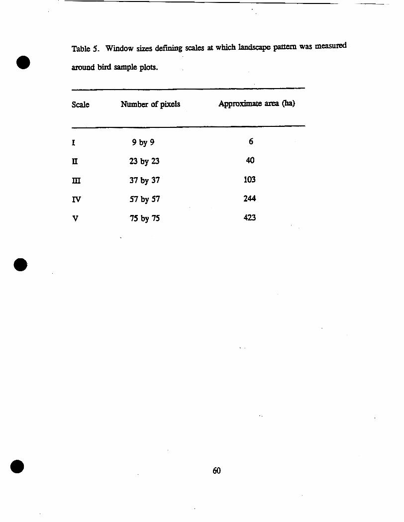
Table 5. Window sizes defining scales at which Landssapc paDcm Was n ~ e a s d

mund bird sample plots.

Scale Number of pixels Appr~- area (ha)

Table 6. Indices of landscape pattern calculated for each window size, for all 66 plots.

Category Index Definition Interpretation

Composition Patch Type Diversity Area of each percent area of Covertype composition

covertype each covertype

Configuration Number of Patches Total number of Count of all patches Fragmentation

patches in the landscape

Association/Dispersion Relative Contagion Given two randomly ,chosen Extent of aggregation or of patches (RC) cells, cell(i) and cell(j): clumping.

P(cell(i) adjacent to cell@

Patch complexity Fractal Dimension (dlfd) dlfd = 2 * slope of the Edge complexity. regression line of log(am) dlfd = 1, simple shape against logwrimeter) dlfd = 2, comple~ shape

Perimetertarea ratio Total perimeterltotal area Relative edge complexity

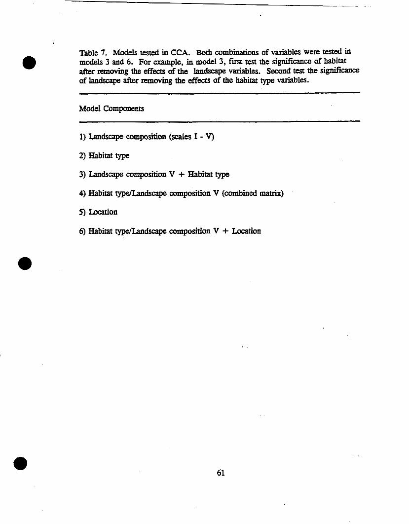
Table 7. Models tested in CCA. Both combinations of variables were tested in a models 3 and 6. For example, in model 3, f m test the significance of habitat after removing the effezts of the landscape variables. Second test the significaace of landscape after removing the effects of the habitat type variables.

Model Components - --

1) Landscape composition (scales I - V) 2) Habitat type

3) Landscape composition V + Habitat type

4) Habitat typ&mdscape composition V (combined matrix)

5) Lncation

6) Habitat -ciscape composition V + Location

Table 8. Landscape variables used in CCA. Variables with -t p-values @

c 0.05) are indicated for each scale. Sigificance was using forward

selection with Monte Carlo pennutation ttso (n = 9999) in CANOCO.

Landscape variable

Midgrass / mixed grass

Midgrass / sh~rtgrass

Wetland / riparian

Non-native hay / pasture

Native tallgrass

Urban vegetation, buildings and pavement

Number of patches

Contagion

Scale

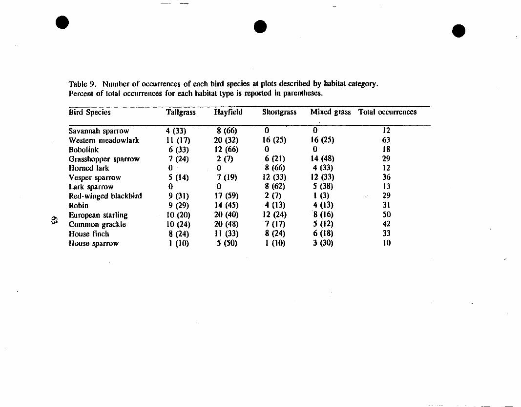
Table 9. Number of occurrences of each bird species at plots described by habitat category. Percent of tolal occurrences for each habitat type is reported in parentheses.

Bird Species Tallgrass Hayfield Shortgrass Mixed grass Total occurrences

Savannah sparrow 4 (33) 8 (66) 0 0 12 . Western meadowlark I 1 (17) 20 (32) 16 (25) 16 (25) 63

Bobolink 6 (33) 12 (66) 0 0 18 Grasshopper sparrow 7 (24) 2 (7) 6 (21) 14 (48) 29 Horned lark 0 0 8 (66) 4 (33) 12 Vesper sparrow 5 (14) 7 (19) 12 (33) 12 (33) 36 Lark sparrow 0 0 8 (62) 5 (38) 13 Red-winged blackbird 9 (31) 17 (59) 2 (7) 1 (3) ..- 29 Robin 9 (29) 14 (45) 4 (13) 4 (13) 3 1 European starling 10 (20) 20 (40) 12 (24) 8 (16) 50 ' Common gmckle 10 (24) 20 (48) 7 (17) 5 (12) 42 House finch 8 (24) 1 I (33) 8 (24) 6 (18) 33 House sparrow 1 (10) 5 (50) 1 (10) 3 (30) 10

Table 10. Results of logistic regression analysis for single species. Larger p-values indicate better model fit. Smaller AICC values indicate a better model choice. Models included presencelabsence for individual species as the dependent variable, and landscape variables as independent variables.

Species Variable tested (scale) p-va lue t, AICC

Homed lark number of patches (I) 0.76 midgrasslmixed grass (m) 0.76 urban (V)

House sparrow uhan (m) 0.92 midgrass/shortgrass (m)

E Bobolink tallgrass (I) 0.95 urban (m)

Lark sparrow midgrass/shortgrass O 0.51 midgrass/shortgrass (m) 0.97 urban (III, V)

FCIQ\04 t'.c'.?0909 O O O C O

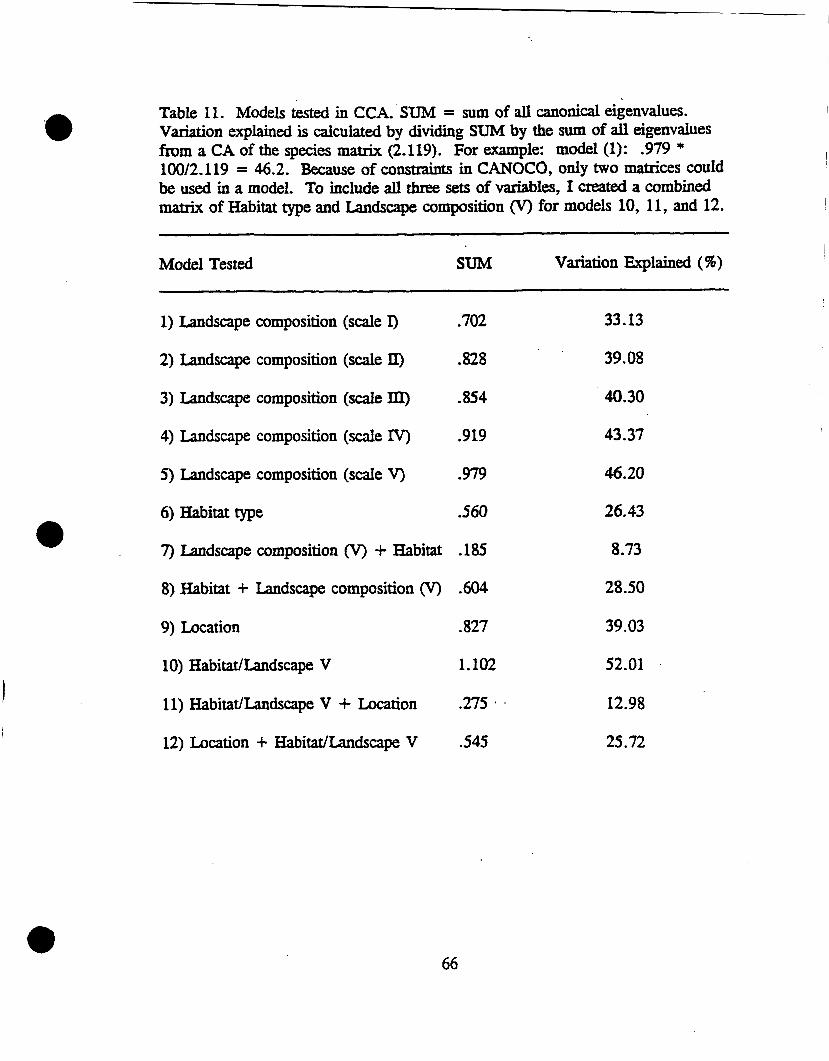
Table 11. Models tksted in CCA. S U M = sum of al l canonical eigenvalues. Variation explained is calculated by dividing S U M by the sum of all eigenvalues from a CA of the species matrix (2.119). For example: model (1): .979 * 10012.119 = 46.2. Because of constraints in CANOCO, only two matrices could be used in a model. To include all three sets of variables, I created a combined matrix of Habitat type and Landscape composition (V) for models 10, 11, and 12.

-

Model Tested SUM Variation Explained (%)

1) Landscape composition (scale I) .702 33.13

2) Landscape composition (scale ll) .828 39.08

3) Landscape composition (scale III) .854 40.30

4) Landscape composition (scale IV) .919 43.37

5) Landscape composition (scale V) .979 46.20

6) Habitat type -560 26.43

7) Landscape composition (V) + Habitat .I85 8.73

8) Habitat + Landscape composition (V) -604 28.50

9) Location .827 39.03

10) Habitat/Landscape V 1.102 52.01

11) HabitatILandscape V + Location .275 . 12.98

12) Location + EXabitat/Landscape V .545 25.72

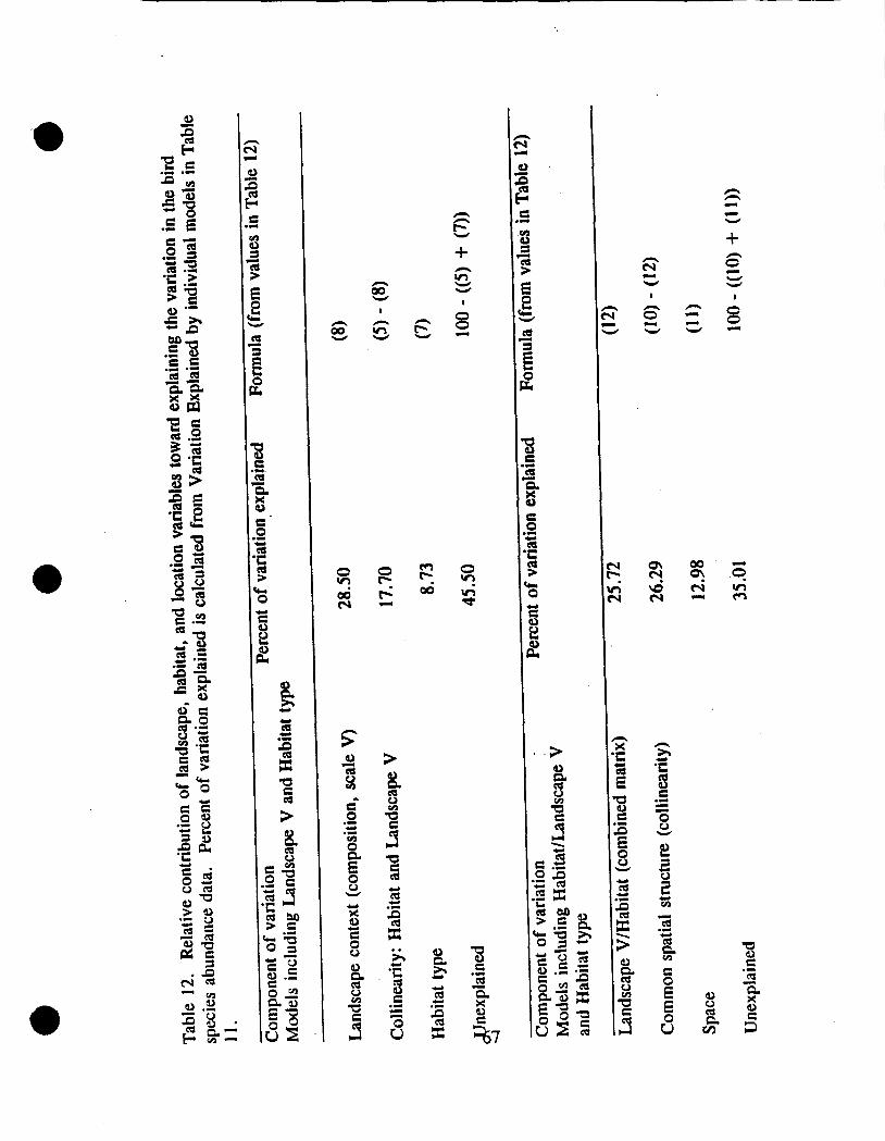
Figure 1. Map extent for analysis of landscape pattern in grasslands and urban areas near Boulder, Colorado. The stippled area on the western edge represents the Front Range of the Rocky Mountains. The polygons surrounding the city of Boulder are Open Space properties. Urban areas are shaded.

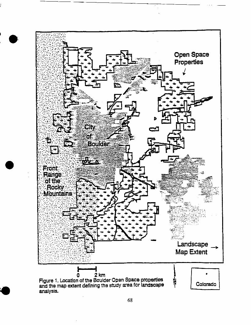
0 2 km Figure 1 . Location of the Boulder Open Space pmpetties and the map extent defining the sWdy area for landscape

Figure 2. Three masks were used to aid in classification of the satellite image. The tallgrass mask included the area southwest of the city of Boulder, where most of the native tallgrass areas occur. The northeast mask covered the urban and suburban areas and the agricultural regions in the northeastern portion of the study area. The southwest mask included the foothills and the upland grassland areas to the south and north of the city of Boulder.

Figure 3. Example of an ordination diagram. This simplified ordination diagram shows one gradient, represented by a line that is proportional to its importance to the ordination. The mean of the gradient occurs at the origin. The lower end of the gradient (not shown in most diagrams) is represented by a dashed line. Species points (shown as dots) are located in the center of the species' distribution along the gradient. A perpendicular line drawn From the species point to the gradient line locates the center of the species distribution for each species along any gradient in the diagram.

Figure 4. Land cover map of the study area, including Boulder, Colorado Open Space grasslands and surrounding lan*. The map legend is shown on the following page.

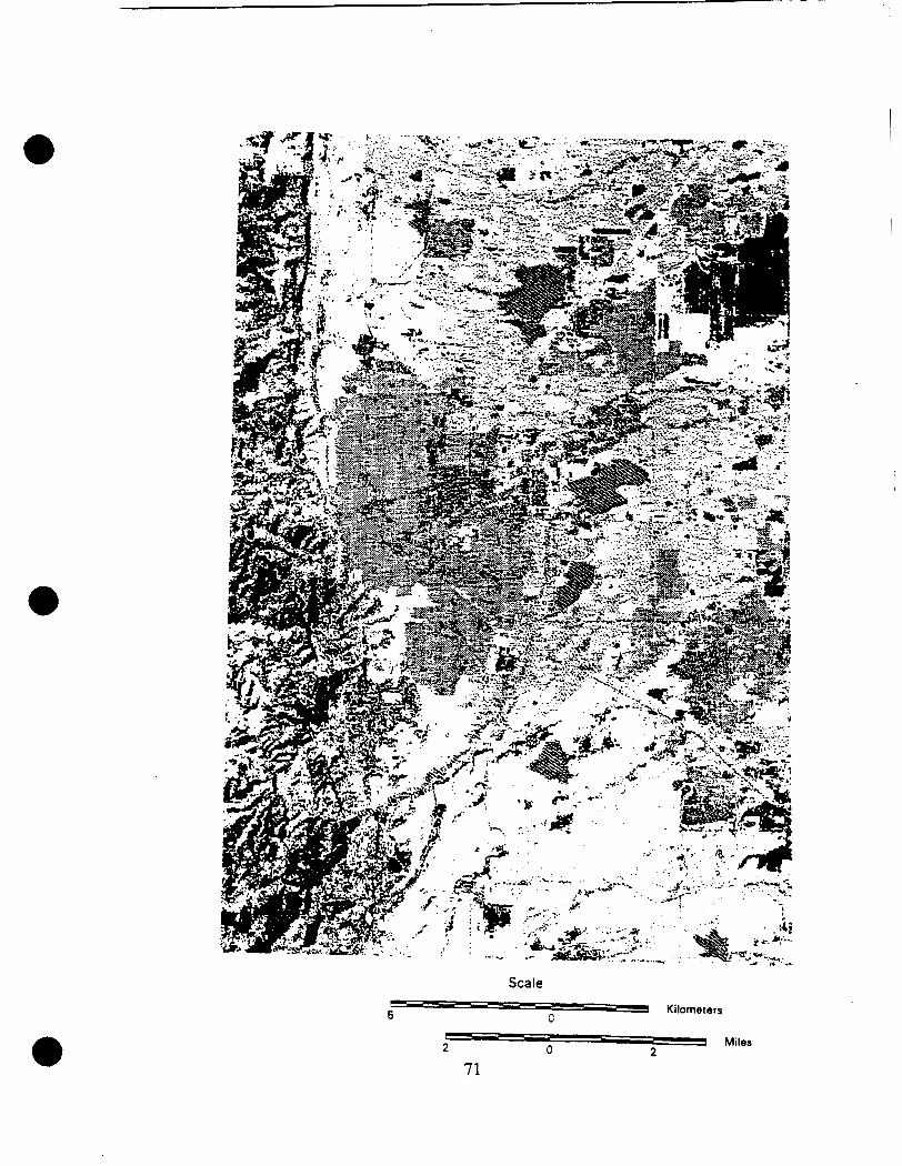
Scale

63 C Kilometers

2 1 2 Miles

71

Class-Names Class-Names

Wetland/riparian

Water Midgrass/shortgrass

Conifer -27-q. :6+&,. - 7.-;

+ak:,?,.;: Non-native hay/pesture

Ponderosa pine shrub/savanna Ponerosa pine forest/woodland

Midgrass/mixed grass Shrubs

Class-Names

Bare rock/soil

Buildings/paved

Urban vegetation

Native tallgrass (wetter)

$m#&q Native tallgrass (drier)

Ill 11-4

Figure 5c. Box plots of cover type distribution at scale 111. The horizontal line in the interior of the box is located at the median of the data. The whiskers extend to the extreme values of the data.

Figure 5d. Box plots of cover type distribution at scale IV. The horizontal line in the interior of the box is located at the median of the data. The whiskers extend to the extreme values of the data.

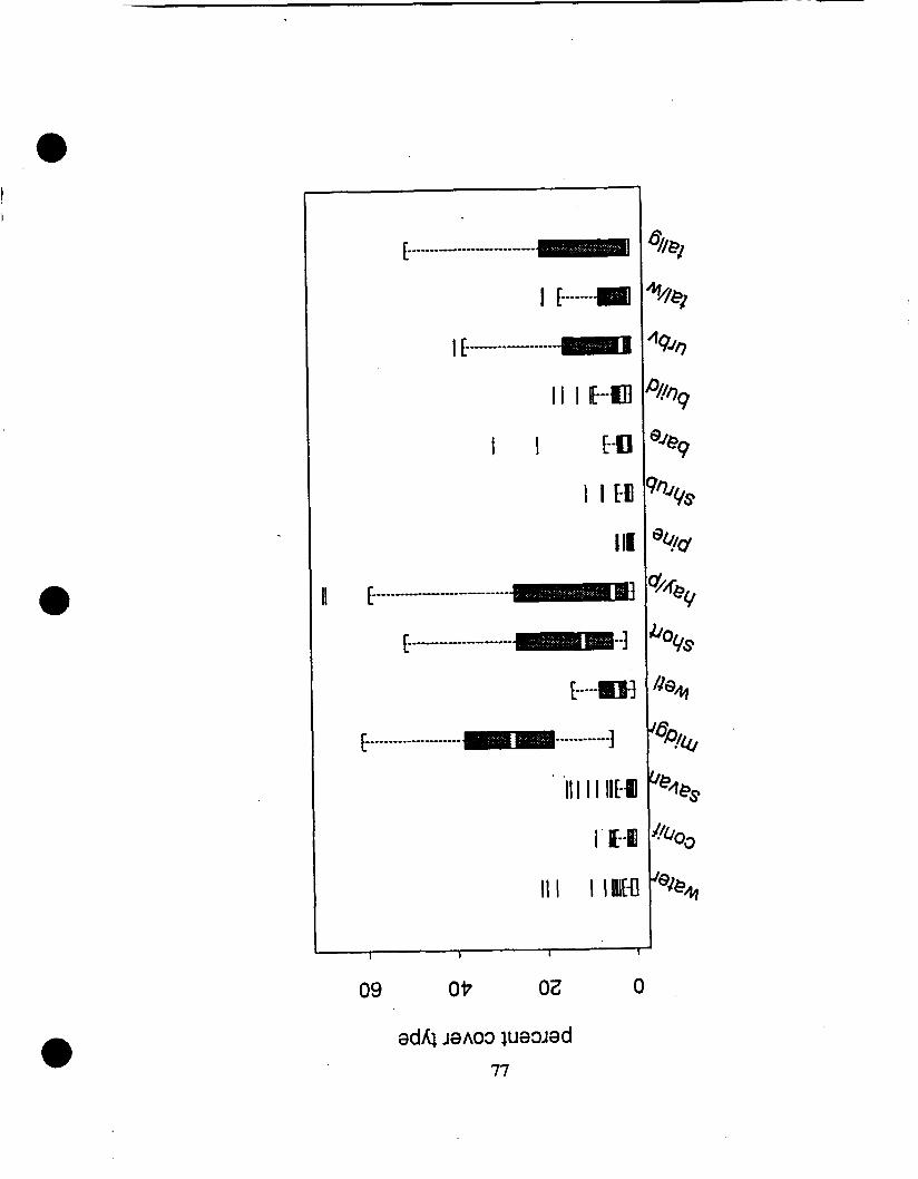
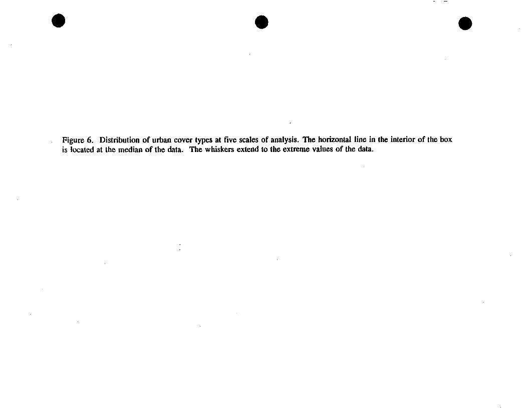
Figure 6. Distribution of urban cover types at five scales of analysis. The horizontal line in the interior of the box is located at the median of the data. The whiskers extend to the extreme values of the data.

DLFD

I ' 11 I l l IV v

NUMBER OF PATCHES

OOE 002 001 0s 0

Figure 8. Geographic distribution of four grassiand bird species in the study area. The Savannah Sparrow and Bobolink overlapped in distribution, but were only observed in tallgrass or hayfield plots. The Lark Sparrow and the Homed lark occurred exclusively in mixed grass and shortgrass plots, but were never observed at the same plots.

;:&

BOBOLINK . .

A SAVANNAHSPARROW 1-1 HORNED LARK 0 2krn LARK SPARROW

MOUtiVdS HVNNVAVS

O'E

58

HORNED LARK

VESPER SPARROW

Figitre 10. Scatter plots of Bobolink, Savannah Sparrow, Lark Sparrow and Horned Lark abundance (y-axis) and percent lowland or upland grassland in the landscape at scale 111. The first two species occurred only in lowland types, and the latter two occurred only in upland grass types. This association carried over in the species' relationships to landscape pattern.

Z' L 8'0 P'O 0'0

MOtltlVdS HVNNVAVS

O'E 0'2 O'C 0'0

Figure I la. Ordination diagram resulting from CCA analysis using variables selected with forward selection at scale I. Species points are dots, and lines represent gradients identified in the ordination. The eigenvalues were 0.485 (axis 1) and 0.145 (axis 2). CONTAGIO = Contagion, TALLGTOT = Tallgrass (percent composition), HAYPASTU = Non-native haylpasture (percent composition), NUMPATCH = Number of patches, MIDGRMIX = Midgrasslmixed grass. See Table 1. for bird species names. Midgrasslshortgrass gradient is coincident with tnidgrasslmixed grass at scale I. Four species points are not labelled: Savannah Sparrow species point is located on the TALLGTOT gmdient, House Finch and Anierican Robin are located by the Starling, and Grasshopper Sparrow is located by the Lark Sparrow.

Figure 1 lc. Ordination diagram resulting from CCA analysis using variables selected with forward selection at scale V, Species points are dots, and lines represent gradients identified in the ordination. The eigenvalues were 0.471 (axis 1) and 0.21 1 (axis 2). WETLRIPA = Wetlandtriparian (percent composition). Red-winged blackbird point is near Bobolink, Starling, Robin and House Pinch points are very close to Grackle.

Figure 12. Spatial patterns of grassland and urban cover types. Upland grasslands (mixed grass and shortgrass) occur in large contiguous areas in the south-central and north-eastem areas of the map. Non-native haylpasture cover types are restricted to the northeastern portion of the map, and tallgrass extends into the central area, just southeast of Boulder. The development of urban areas has occurred in a large, central area, and in several smaller clusters across the landscape.

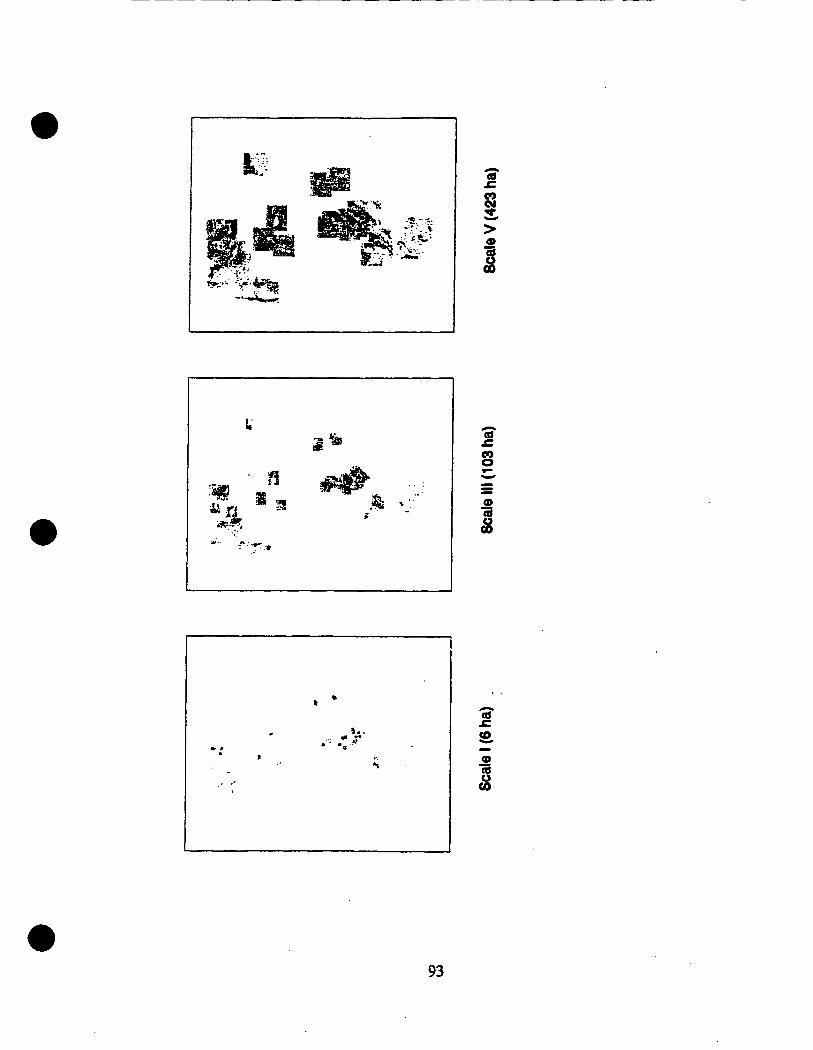
Appendix 1. Examples of signatme plots used in image classEcation.

. . Layer

- midgrass les - midgrass mor

. . Layer

. . Layer

- ppine forest - ppine forest - ppine forest I

Layer

s h r u b s 18

I I

. . Layer

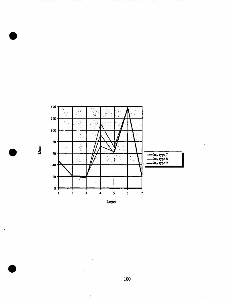
I 2 3 4 5 6 7 . .

Layer

Appendix 2.

Bird species

savannah meadow bobolink grasshop hornedlark vesperspa larksparro redw inged amrobin eurstarling cograc kle housefinch housespar

Data files used in analysis.

Savannah Sparrow Western Meadowlark Bobolink Grasshopper Sparrow Homed Lark Vesper Sparrow Lark Sparrow Red-winged Blackbird American Robin European Starling Common Grackle House Finch House Sparrow

~ y y y o o o o q ~ ~ * o o ~ ~ a 0 q o o o " ! O O O O ~ * [ ' . ~ - 2 - 2 c o o 0 G

0 0 0 0 o o o o a o a

i E

. 9 - 0 y 0 0 0 0 0 0 0 - 0 0 ~ q 0 0 - 0 9 9 0 0 0 ~ ~ y ~ ~ 0 ' + r ~ o q

1" 0 0 0 0 d 0.0 O O O O O 0 - 0

m

~ m ~ m ~ ~ 4 4 q q q 0 q y ~ ~ q q ~ 0 0 m d y ~ q q 0 0 0 0 - ~ + ~ ~ m ~ - - ~ ~ o - o o o r v o o o t w o * 0 o o 0 - 0 o o - 3 3 P)

plot no. I 2 3

4 5 6 7 8 9 10 1 1 12 13 14

x-coord 30579 18 3058049 3058775 3059866 3059366 3063806 30649 18 306382 1 3064463 3066364 3066693 3061719 3062363 3065860 3065922 3070500 3070101 3071612 3077386 30773 17 3075179 307738 1 3098308 3098147 3074328 3074982 3072570 3070 105 3069777 308 1756 3080658 309 1424 3092209

ycoord

1262 144 1262782 126500 1 126882 1 1269140 127 1574 1271643 1272276 1272702 127 1828 127 1206 1277934 1277705 1275591 1275990 1272898 1273349 1278202 1278617 1278035 1275923 1275457 1266853 1266037 1263758 12637511 1257346 1229743 1229810 1259897 1259853 1245936 1245937

plot no. 34 3 5 36 37 3 8 39 40 4 1 42 43 44 45 46 47 48 4 9 50 5 1 52 53 54 55 56 57 58 59 60 6 1 62 63 64 65 66

x-coord 3078549 3080265 307974 1 3078758 3077638 3093787 3093833 308080 1 3081036 3078967

3079691 3080068 3082655 3082899 3083492 308 1036 3082483 3081473 3082703 3083473 3072738 307 1697 3072 179 307 1703 3074464 3074393 307 1956 30731 1 1 3072979 3077453 3077986 3078 193 3093289

Appendix 2. Continued. Habitat type categorical data for the 66 sample plots.

plot no. 1 2 4 5 6 7 8 9

10 11 12 13 14 1 S 16 17 19 20 2 1 22 23 24 25 26 28 29 30 31 32 33 34 35 36 37 38 39

mixed grass 1 1 1 1 0 0 0 0 0 0 1 1 0 0 0 0 0 0 0 0 1 1 0 0 1 1 0 0 0 0 0 0 0 0 0 0

Appendix 2. Continued.

Landscape data for Scale I.

(Key applies to all scales)

water percent water conifer percent conifer forest savannah percent Ponderosa pinelshrub savannah midgrasslb percent midgrasslmixed grass wetlandlriparian percent wetlandlriparian midgrassmb percent midgrasslshortgrass haylpasture percent non-native haylpasture ponderosa pine percent Ponderosa pine forest shrubs percent shrubs bare soil percent bare soillrock buildingslpaved percent buildingslpaved urban veg percent urban vegetation tallgrasslwet percent native tallgrass (wetter) tallgrass percent tallgrass area (ha) area of the geometric sampling window num patches number of patches dlfd double log fractal dimension contagion percent contagion perimeterlarea perimeter of all patches divided by area (ha) tallgrass(total) sum of tallgrass and tallgrass (wet) urban(tota1) sum of urban veg and buildingslpaved

~ o C a ~ o c o o ~ o 0 ~ o - o o o o o o o o o o o o o o o o o o o o m w o o o l - o o * o s 0 8 q q q q q q q q q q 0 0 ~ 0 0 0 q 0 ~ d ~ 4 d d d ~ d d ~ 4 ~ G ~ ~ o o o o o o o o o 0 0 0 0 0 0 0 0 o U)

plot no. 34.00 35.00 36.00

37.00 38.00 39.00 -40.00

4 1 .OO 42.00

water 0.00 0.00 0.00

0.00 0.00 0.00 0.00

0.00 0.00

0.00 0.00 0.00

0.00 0.00

0.00

0.00 0.00 0.00

0.00 0.00 0.00 0.00 0.00 0.00 0.00 0.00 0.00 0.00

0.00 0.00 0.00

0.00

0.w

conifer 0.00 0.00 0.00

0.00 0.00 0.00 0.00

0.00 0.00

0.00 0.00 0.00 0.00

0.00 0.00

0.00 0.00

0.00

0.00 0.00 0.00 0.00 0.00 0.00 0.00 0.00 0.00 0.00 0.00 0.00 0.00

0.00

0.00

savannah 0.00 0.00 0.00

0.00 0.00 0.00 0.00

0.00 0.00 0.00 0.00 0.00 0.00

0.00 0.00

0.00 0.00

- 0.00

0.00 0.00 0.00 0.00 0.00 0.00 0.00 0.00 1.23 0.00

4.94 0.00 0.00

0.00

0.00

wetlandrip 0.00

12.35 9.88

13.58 6.17 a

0.00

0.00 0.00 2.47

8.64 12.35 2.47

12.35 13.58 13.58

1.23 0.00 0.00 0.00 0.00

14.81 0.00 3.70 7.4 1 1.23 0.00 0.00 0.00 0.00 0.00 0.00

0.00

0.00

midgrassmb 0.00 1.23 0.00

0.00 0.00 1.23 0.00

0.00 0.00

0.00 0.00 0.00 0.00

0.00 0.00

0.00 0.00

0.00 2.47 2.47 4.94 0.00 0.00 1.23 1.23 1.23 0.00

12.35 64.20

74.07 77.78

71.60

0.00

haylpasture ponderosa pine 7.4 1 0.00 0.00 0.00 0.00 0.00

0.00 0.00 3.70 0.00

49.38 0.00

88.89 0.00 1.23 0.00 0.00 0.00

0.00 0.00 0.00 0.00 0.00 0.00 0.00 0.00 0.00 0.00

0.00 0.00

2.47 0.00 0.00 0.00

0.00 0.00 0.00 0.00 0.00 0.00

7.4 1 0.00 0.00 0.00 1.23 0.00 0.00 0.00 1.23 0.00 0.00 0.00 0.00 0.00 0.00 0.00 0.00 0.00 0.00 0.00 0.00 0.00

0.00 0.00

83.95 0.00

shrubs 0.00 0.00 0.00

0.00 0.00 0.00 0.00 0.00 0.00

0.00 0.00 0.00 0.00 0.00

0.00

0.00 0.00

0.00 0.00 0.00 0.00 0.00 0.00 0.00 0.00 0.00 0.00 0.00 0.00 0.00 0.00

0.00

0.00

bare soil 0.00 0.00 0.00

0.00 0.00 0.00

0.00 0.00 0.00 0.00 0.00 0.00

0.00 0.00

0.00 0.00 0.00

0.00 0.00 0.00 0.00

0.00 0.00 0.00 0.00 0.00

0.00 0.00 0.00 0.00 2.47

2.47

0.00

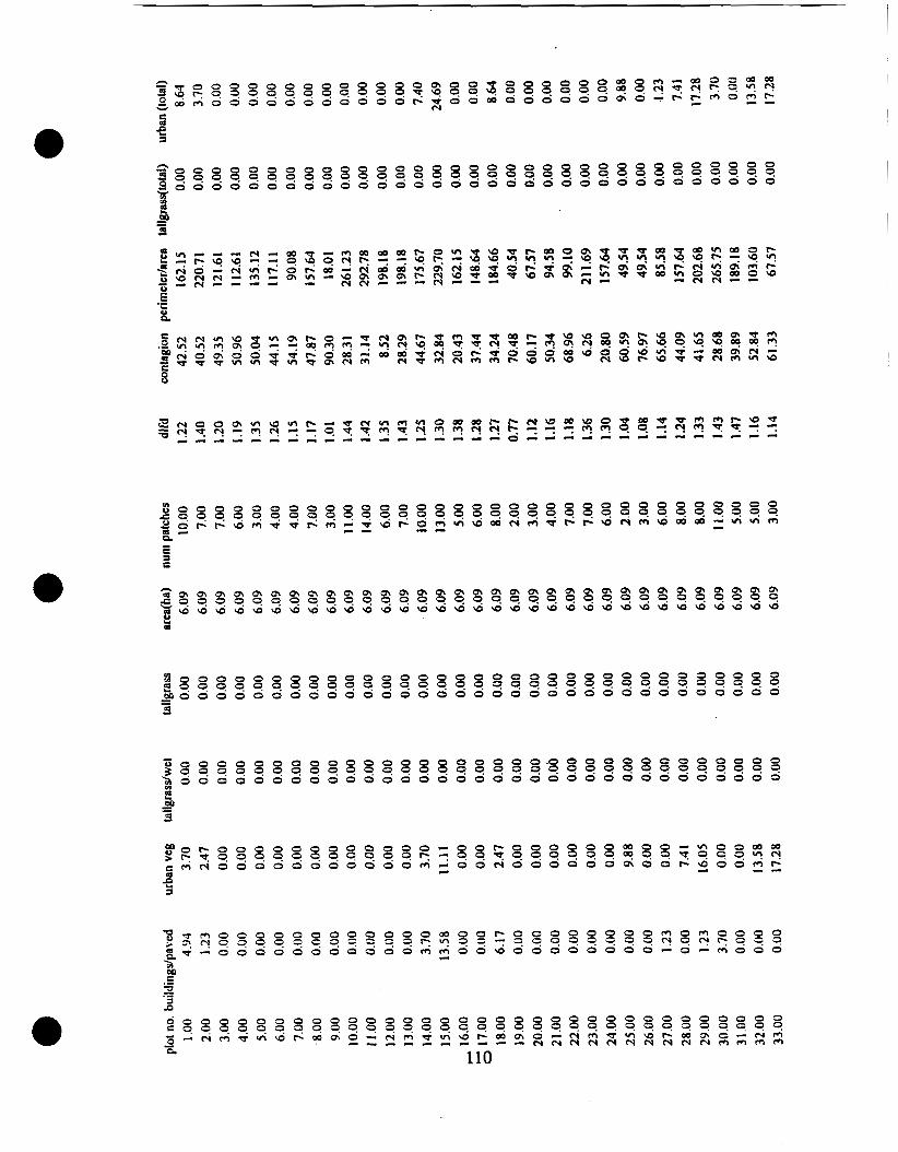
plot no. 1 .oo 2.00 3 .OO 4.00 5.00 6.00

, 7.00 8.00 9.00

10.00

water c

3.40 0.00 0.00 0.00 0.00 0.00 0.00 0.00 0.00 0.00

0.00 0.00 0.00 2.27

3.02 0.00

0.00 0.00

0.00 0.00 0.00 0.00 0.00 0.00 0.00 0.00

10.02 0.00 0.00

0.00 0.00

0.00

0.00

savannah 0.19 0.19 0.95 0.00

0.00 0.00

0.00 0.00 0.00 0.00

0.00 0.00 0.00 0.00

0.00 0.00

0.00

. 0.00

. 0.00 0.00 0.00 0.00 0.00 0.00 0.00 0.00 0.00 4.16 3.59 0.00 0.00

0.00 0.00

midgrasslb 28.73 34.97 38.37 60.68

57.28 32.89

39.13 27.03 15.12 24.76

24.95 58.79 66.73 38.94

39.32 44.23

44.99 14.37

34.59 21.36 13.23 13.99 58.03 70.70 6.05 8.5 1

32.89 4 1.02 37.24

26.09 47.26

6.24 8.13

hey/pasture ponderosa pine 0.00 0.38

0.00 0.00 0.00 0.00 0.00 0.00

0.00 . 0.00 0.00 0.00

0.00 0.00 0.00 0.00 0.00 0.00

27.60 0.00

32.70 0.00 0.00 0.00 0.00 0.00 0.19 0.00

0.38 0.00

3 1.38 0.00 37.62 0.00

24.57 0.00 58.98 0.00 73.91 0.00 76.56 0.00 72.78 0.00 0.00 0.00 0.00 0.00

85.44 0.00 80.34 0.00

25.14 0.00 0.00 0.00 0.00 0.00

55.01 0.00 32.89 0.00

57.28 0.00

5 1.94 0.00

shrubs 1.70 2.84 1.13 0.76

1.13 4.35 2.27 8.51 8.70 0.38

1.32 7.18 6.43 0.00

0.00

0.00 0.00

0.00 0.00 0.00

0.00 0.00 0.00 0.00 0.00 0.00

0.00 0.76 0.57 0.00 0.00

0.00 0.00

bare soil 0.00 0.00 0.95 7.18 1.89 7.37 8.70 7.94 6.43

10.78

7.18 4.73 1.5 1 2.46 2.08

1.13 0.00

9.45 0.19 0.00 0.00 0.38

10.96 3.02 0.95 0.95

3.59 0.00 0.00 0.19 0.19

0.00

0.19

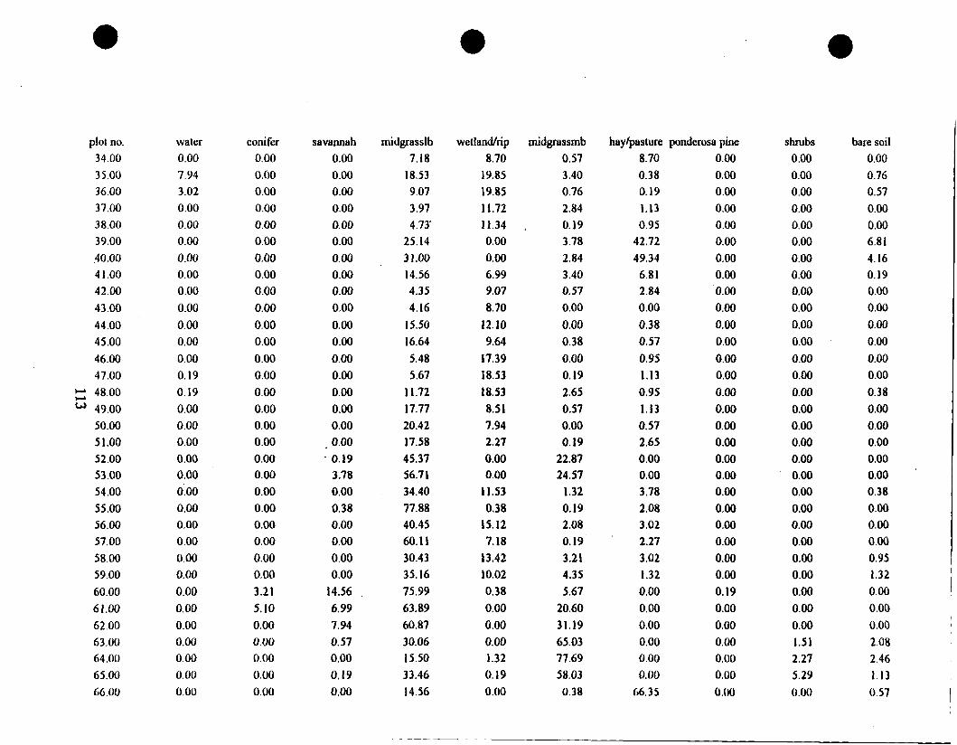
plot no. 34.00

35.00 36.00 37.00 38.00 39.00 40.00 4 1 .OO 42.00

43.00

44.00 4 5 .OO 46.00 47.00 48.00 49.00 50.00

5 1 .oo 52.00 53.00 54.00 55.00 56.00 57.00 58.00 59.00

60.00 61.00

62.00 63.00 64.00 65.00 66.00

water 0.00 7.94 3.02 0.00 0.00 0.00 0.00 0.00 0.00

0.00

0.00 0.00

0.00 0.19 0.19 0.00 0.00 0.00 0 .oo 0.00 0.00 0.00 0.00 0.00

0.00 0.00

0.00 0.00

0.00 0.00 0.00 0.00 0.00

conifer 0.00 0.00 0.00 0.00 0.00 0.00 0.00 0.00 0.00

0.00

0.00 0.00

0.00 0.00

0.00 0.00 0.00 0.00 0.00 0.00 0.00 0.00 0.00 0.00 0.00 0.00

3.21 5.10 0.00 0.00

0.00 0.00 0.00

savannah 0.00 0.00 0.00 0.00 0.00 0.00 0.00

midgrassmb 0.57 3.40 0.76 2.84 0.19 3.78 2.84 3.40 0.57 0.00

0.00 0.38 0.00 0.19

2.65 0.57 0.00 0.19

22.87 24.57

1.32 0.19 2.08 0.19 3.21 4.35 5.67

20.60

31.19 65.03 77.69 58.03 0.38

hay/pasture ponderosa pine 8.70 0.00 0.38 0.00 0.19 0.00

1.13 0.00 0.95 0.00

42.72 0.00 49.34 0.00 6.81 0.00 2.84 0.00 0.00 0.00

0.38 0.00 0.57 0.00

0.95 0.00 1.13 0.00

0.95 0.00 1.13 0.00 0.57 0.00 2-65 0.00 0.00 0.00 0.00 0.00 3.78 0.00 2.08 0.00 3.02 0.00 2.27 0.00 3.02 0.00 1.32 0.00 0.00 0.19 0.00 0.00 0.00 0.00 0.00 0.00 0.00 0.00 0.00 0.00

66.35 0.00

bare soil 0.00 0.76 0.57 0.00 0.00 6.8 1 4.16 0.19 0.00 0.00

0.00

0.00

0.00 0.00

0.38 0.00

0.00 0.00 0.00 0.00 0.38 0.00 0.00 0.00 0.95

1.32 0.00 0.00

0.00 I

2.08 2.46 1.13 0 57 I

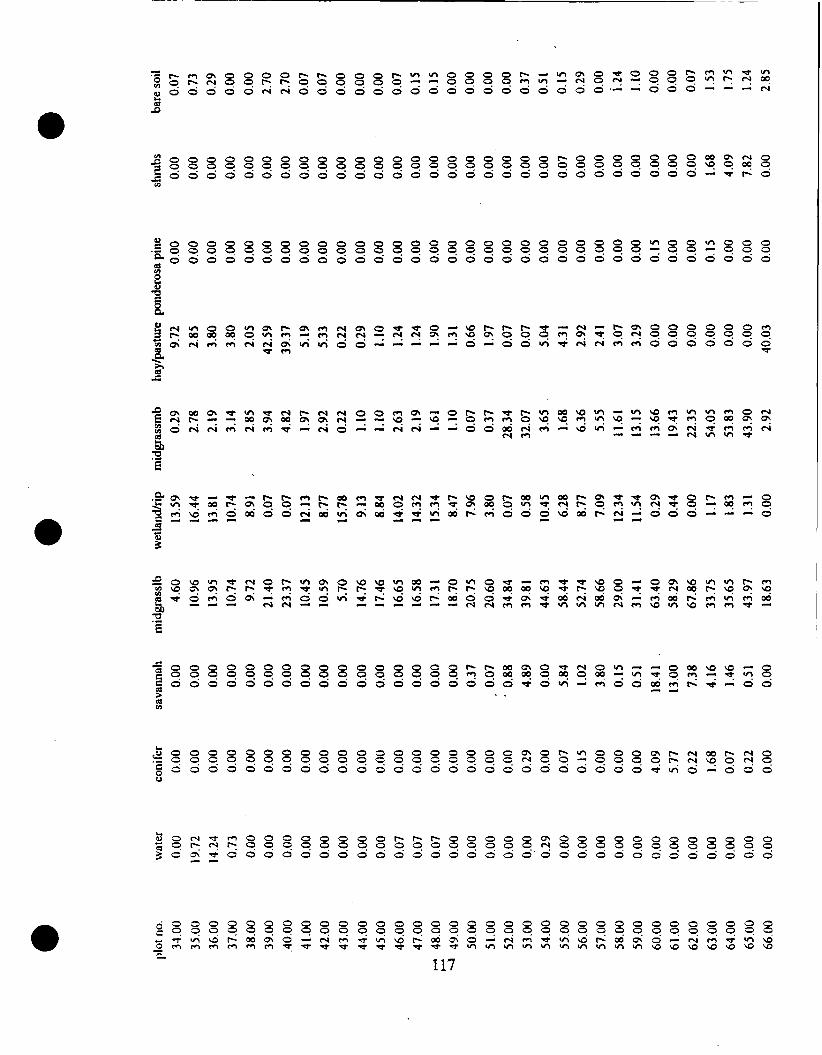
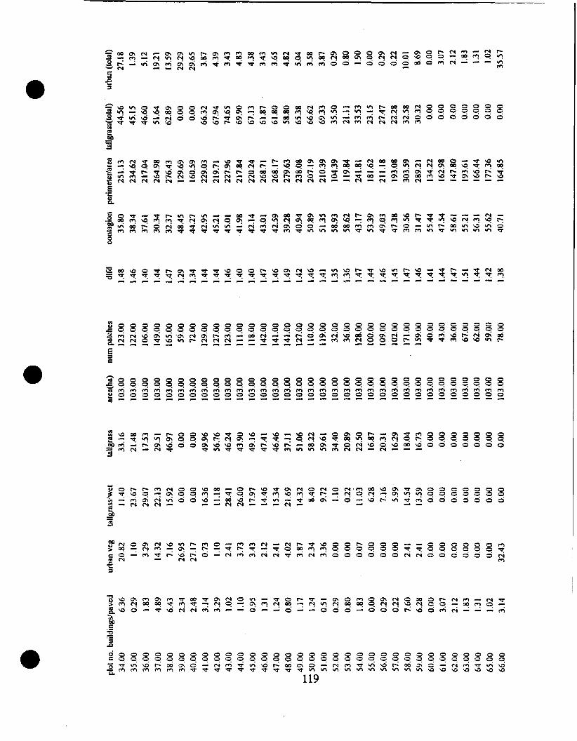
~ m ~ m m u m m m m m ~ m o o ~ m w a w o o m m 5 0 , 0 r n m m ~ ~ w ~ e m E q ? y ~ q q q q q m o q ~ ~ p ~ m o ~ m q ~ t - m a m ~ w u q q ~ o m m m m w w m m m - - - - 4 - + m m k P - & & ~ ~ ~ ~ ~ h h m m m m e 4 - m m m

h - a m v ~ ~ ~ O ~ ~ ~ e ~ m u , - m m ~ m ~ m m - - ~ m O O O O o O ~ J q o ~ m o o y o q ~ q m e + q ? y q m q q ~ o q o o o q o q q S m m ~ \ d r c o o r r i d w m m ~ m m - a a o ~ ~ a m o o o o o o = x m m m v v a $ % G p m m w a m m m m m m C) m m 6

- ~ - v ~ P N m ~ ~ - m m ~ m y m s - ~ O \ O ~ ~ o O e m ~ O ~ ~ * ~ ~ ~

~ ~ , c ? F Y " ~ q y 0 m o w w o p a m - " " o ? $ 9 - - - m m 4 v w ~ m & b ~ A & l A & m A & ~ d - d - - ~ d d ~ s ' ~ n f m N

3

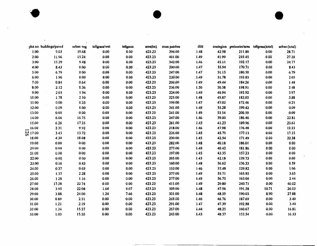
plot no. buildingdpaved 1 .OO 9.03 2.00 11.96 -

3.00 15.29 4.00 8.43 5.00 6.79 6.00 1.96 7.00 0.84 %.OO 2.12 9.00 2.03

10 .OO 1.78 1 1 .oo 0.00 12.00 0.09 13 .OO 0.09 14.00 6.06 1 5.00 6.26

c.. 16.00 2.3 1 17.00 3.43 1 8 .OO 4.30 19.00 0.00 20.00 0.00 2 1 .oo 0.00 22.00 0.oq

' 23.00 0.16 24.00 0.37 25.00 1.37 26.00 1.28 27.00 17.28 28.00 3.95 29.00 3.88 30.00 0.89 3 1 .oo 1.2 1 32.00 1.24 33.00 1.03

urban veg 19.68 15.24 9.48 0.00 0.00 0.09 0.64 0.36 1.94 2.10 0.25 0.00 0.00

16.75 17.35 9.92

13.72 18.08 0.00 0.00 0.00 0.00 0.43 0.69 2.28 1.16

22.74 22.08 24 .OO 2.51 2.19

15.57 15.50

tallgrass 0.00 0.00 0.00 0.00 0.00 0.00 0.00 0.00 0.00 0.00 0.00 0.00 0.00 0.00 0.00 0.00 0.00 0.00 0.00 0.00 0.00 0.00 0.00 0.00 0.00 0.00 0.00 9.07 7.66 0.00 0.00 0.00 0.00

num patches 394.00 40 1 .OO 342.00 200.00 247.00 22d.00 200.00 236.00 224.00 225.00 199.00 24 1 .OO 24 1 .OO 247.00 26 1 .OO 2 18.00 226.00 230.00 282.00 277.00 197.00 205.00 160.00 153.00 277.00 277.00 41 1.00 309.00 30 1 .OO 269.00 291 .OO 267.00 243.00

dlfd contagion perimcterlarea 1.48 42.98 21 1.80 1.49 4 1.99 219.45 1.46 45.1 1 192.17 1.47 55.94 170.7 1 1.47 51.15 180.50

. I .49 51.78 193.85 1.49 49.44 184.26 1 .SO 50.38 198.91 1.49 46.94 195.92 1.48 45.87 182.05 1.47 47.02 172.46 1.49 55.28 199.42 1.49 53.54 200.59 1.46 39.00 186.40 1.45 4 1.23 189.96 I .46 47.98 176.48 1.45 45.79 177.13 1.45 42.54 171.49 1.48 40.18 186.01 1.49 40.42 18 1.86 1.45 43.35 157.23 1.43 42.18 139.73 1.48 56.62 136.23 I .46 57.48 129.82 1.49 55.7 1 165.85 1.49 56.75 163.00 1.49 29.80 240.7 1 1.48 47.96 191.58 1.48 48.59 190.03 1.46 46.76 187.69 1.47 47.39 192.88 1.44 48.25 160.67 1.43 48.57 153.54

urban (total) 28.7 1 27.20 24.77

8.43 6.79 2.05 1.48 2.48 3.97 3.88 0.25 0.09 0.09

22.81 23.61 12.23 17.15 22.38 0.00 0.00 0.00 0.00 0.59 1.06 3.65 2.44

40.02 26.03 27.88 3.40 3.40

16.81 16.53