analyzing the relationship of soil moisture and
TRANSCRIPT
University of Nebraska - LincolnDigitalCommons@University of Nebraska - Lincoln
Dissertations & Theses in Natural Resources Natural Resources, School of
Summer 7-24-2015
ANALYZING THE RELATIONSHIP OF SOILMOISTURE AND BIOPHYSICAL VARIABLESIN WET AND DRY SEASONS AT A RAINFEDAND IRRIGATED FIELD IN EASTERNNEBRASKAEric HuntUniversity of Nebraska-Lincoln, [email protected]
Follow this and additional works at: http://digitalcommons.unl.edu/natresdiss
Part of the Environmental Monitoring Commons, and the Water Resource ManagementCommons
This Article is brought to you for free and open access by the Natural Resources, School of at DigitalCommons@University of Nebraska - Lincoln. Ithas been accepted for inclusion in Dissertations & Theses in Natural Resources by an authorized administrator of DigitalCommons@University ofNebraska - Lincoln.
Hunt, Eric, "ANALYZING THE RELATIONSHIP OF SOIL MOISTURE AND BIOPHYSICAL VARIABLES IN WET AND DRYSEASONS AT A RAINFED AND IRRIGATED FIELD IN EASTERN NEBRASKA" (2015). Dissertations & Theses in NaturalResources. 122.http://digitalcommons.unl.edu/natresdiss/122
ANALYZING THE RELATIONSHIP OF SOIL MOISTURE AND BIOPHYSICAL
VARIABLES IN WET AND DRY SEASONS AT A RAINFED AND IRRIGATED
FIELD IN EASTERN NEBRASKA
by
Eric Daniel Hunt
A DISSERTATION
Presented to the Faculty of
The Graduate College at the University of Nebraska
In Partial Fulfillment of Requirements
For the Degree of Doctor of Philosophy
Major: Natural Resource Sciences
(Climate Assessment and Impacts)
Under the Supervision of Professor Brian D. Wardlow
Lincoln, Nebraska
August, 2015
ANALYZING THE RELATIONSHIP OF SOIL MOISTURE AND BIOPHYSICAL
VARIABLES IN WET AND DRY SEASONS AT A RAINFED AND IRRIGATED
FIELD IN EASTERN NEBRASKA
Eric D. Hunt, Ph.D.
University of Nebraska, 2015
Adviser: Brian D. Wardlow Agriculture production, particularly of maize and soybeans, is a major component of
Nebraska’s economy and identity. However, agricultural production in Nebraska faces
increasing challenges. One of the challenges is the potential for excessive groundwater
depletion due to increased demand for food and fuel from irrigated Nebraska crops and
increasing risks of water stress due to climate change. Therefore, it is has become
essential for a deeper understanding of the soil-plant-atmosphere continuum to help
producers make more informed management decisions. One of the most important
variables is soil moisture. Soil moisture is an integral part of the hydrologic cycle and an
essential component in understanding land-atmosphere interactions. Eight years of soil
moisture and biophysical measurements from an irrigated and rainfed maize-soybean
rotation, in growing seasons that ranged from abnormally dry and warm to unusually
moist and cool, add to that understanding. It is shown that soil moisture is an excellent
measure of the effectiveness of precipitation and that timing of precipitation can be as
important as quantity. Dry spells occurred in most seasons in the study period, but the
timing and duration of said dry spells were important. In seasons where adequate
precipitation returned, measured evapotranspiration and gross primary productivity at the
rainfed field increased to close to that of the irrigated field. Therefore, it is implied that
stomatal conductance seemed to return to close to pre-dry spell levels and rainfed yields
were not substantially reduced compared to the irrigated field. However, during a classic
flash drought in the study period, prolonged soil moisture stress led to reduced stomatal
conductance and significantly reduced maize yields. The flash drought case study not

only showed the importance of irrigation during a prolonged dry spell, it also showed the
utility of using short-term drought indices for identifying water stress of a rainfed field.

ACKNOWLEDGEMENTS
There are numerous people to thank throughout this long process. I would
first like to thank my family. This includes my terrific parents, John and Mary Ann
Hunt, and my siblings, Emily Matlock and Brandon Hunt, for their continued
support and encouragement since I began this program back in 2008. I also would
like to thank my wonderful girlfriend, Britany Porter, for her encouragement and
understanding while I finished up over the past year and a half. I also greatly
appreciate her strong work ethic and ability to avoid procrastinating when working
on her own Master’s program at Doane. My extended family members and
Britany’s family have also been supportive and a source of a fun diversion away
from the dissertation when I needed it.
My adviser and committee chair, Dr. Brian D. Wardlow, deserves credit for
good guidance and being a positive role model throughout this process. I especially
appreciate his thorough critique of my writing and letting me find my own way and
work out my own struggles when developing my research proposal. I also admire
the efforts he puts into teaching and of all his research accomplishments since
arriving at UNL as a research associate for the National Drought Mitigation Center.
I would also like to thank my other committee members, Drs. Tim
Arkebauer, Michael Hayes, Anatoly Gitelson, and Ken Hubbard. Your expertise
and guidance was also vital to my success and it was an honor to work with such
accomplished and respected faculty.
The director(s), faculty, and staff within the School of Natural Resources
are top-notch. It has been a pleasure to get to know and work with Dr. John Carroll

over the past two years. His passion for natural resources education and students
and optimistic, assertive attitude will move the School to heights never seen before.
Dr. Don Wilhite also deserves much praise for his efforts serving as director for
most of my time as a graduate student. His professionalism and calm demeanor
were valuable during a time of budget uncertainty and change at the University of
Nebraska-Lincoln. I have several faculty I would like to thank for outstanding
classes: Drs. Betty Walter-Shea, Shashi Verma, Tim Arkebauer, Anatoly Gitelson,
Kent Eskridge, Jim Brandle, Chuck Francis, Al Weiss, Kevin Pope, Pat Shea, and
Tala Awada.
I would also like to thank many School of Natural Resources graduate
students, both past and present. In no particular alphabetical or chronological order:
Drs. Crystal Stiles, Nathan Healey, Heidi Adams, John Quinn, Brenda Pracheil,
Teresa Donze-Renier, Jane Okalebo, Kevin McVey, Anthony Nguy-Robertson,
Saadia Bihmidine, Sharmistha Swain and Rebecca Howser, Brittany Potter, Adam
Yarina, Jeff Nothwehr, Natalie Umphlett, Ramesh Languini, Jeff Hartman, Babak
Safa, Mikal Stewart, Aaron Young, Becky Young, William “B.J. Baule, Carla
Ahlschwede, Kim Laing, Erik Laing, Luis Ramirez, Katie Shook, Andrew Shook,
Melissa Widhalm, Sandra Jones, Juliana Dai, Karla Jarecke, Cara Whalen, Maggi
Sliwinski, Ashley Alred, Katie McCollum, Katie Lawry, Tracie Lorenzo, William
Avery, Catie Finkenbiner, and others I’m likely forgetting. It was an honor to serve
as the SNR Graduate Association Chair, the SNR Graduate Committee
Representative, and for two years on the UNL Graduate Student Association.

Service to others is always rewarding and I’m proud of my accomplishments in
that realm.
In the late fall of 2011 I received a Facebook message from Sandra Jones
asking if I would be interested in a job. I knew balancing work and a dissertation
would be a challenge but it was a risk I had to take. On a warm Tuesday in March
2012, I began working for Atmospheric and Environmental Research, Inc. as a sub-
contractor for Air Force Weather. Since that time I have also worked a bit with the
United States Army Corps of Engineers Cold Regions Research Laboratory and
more recently with the High Plains Regional Climate Center and have come to
admire and respect my colleagues at NASA-GSFC, NCAR, NOAA, and the UK
Met Office.
I have learned so much from my co-workers and colleagues and there are
several I would like to thank directly: Drs. Rebecca Adams-Selin, Marc Hidalgo,
Jeff Cetola, Jerry Wegiel, Christa Peters-Lidard, Mike Ek, Sujay Kumar, Kristi
Arsenault, Joe Santanello, Ken Harrison, Tim Nobis, Martha Shulski, Trenton
Franz and Mark Conner, Nate Wright, Chris Frank, Ryan Rughe, Eddy Hildebrand,
Steven Bliujus, Rich Butler, Glenn Creighton, James Geiger, Tricia Lawston and
Samantha Ashton.
The members at First Plymouth United Church of Christ have also been a
positive influence on my life in recent years. In particular, I’d like to thank Revs.
Jim Keck and Barb Smisek for inspirational and challenging sermons and to Linda
Schwartzkopf, Mike Fultz, Lou Lau, Lyda Snodgrass, Emily Snodgrass, Mary

Snodgrass, Dave Snodgrass, and Jeff Sheldon for welcoming to their coffee group
after the 9:00 service on Sunday.
Finally, I’d like to thank some other friends who have been a positive
influence throughout this process: James Augustyn, Eric Martin, Steve Howser,
Skyler Swisher, Kevin Selin, Kyle Laughlin, Ken Taylor, Brittany Hergott, Matt
Maw, Amanda Mikesh, Brad Erickson, Mark Sessing, Heather Sessing, Angelyn
Hobson, Lynn Baringer, Airey Baringer, Clark Payne, Alison Svercek, Jim
Southard, Amber Caylor, Josh Stiles, and Lynn Peterson.
i
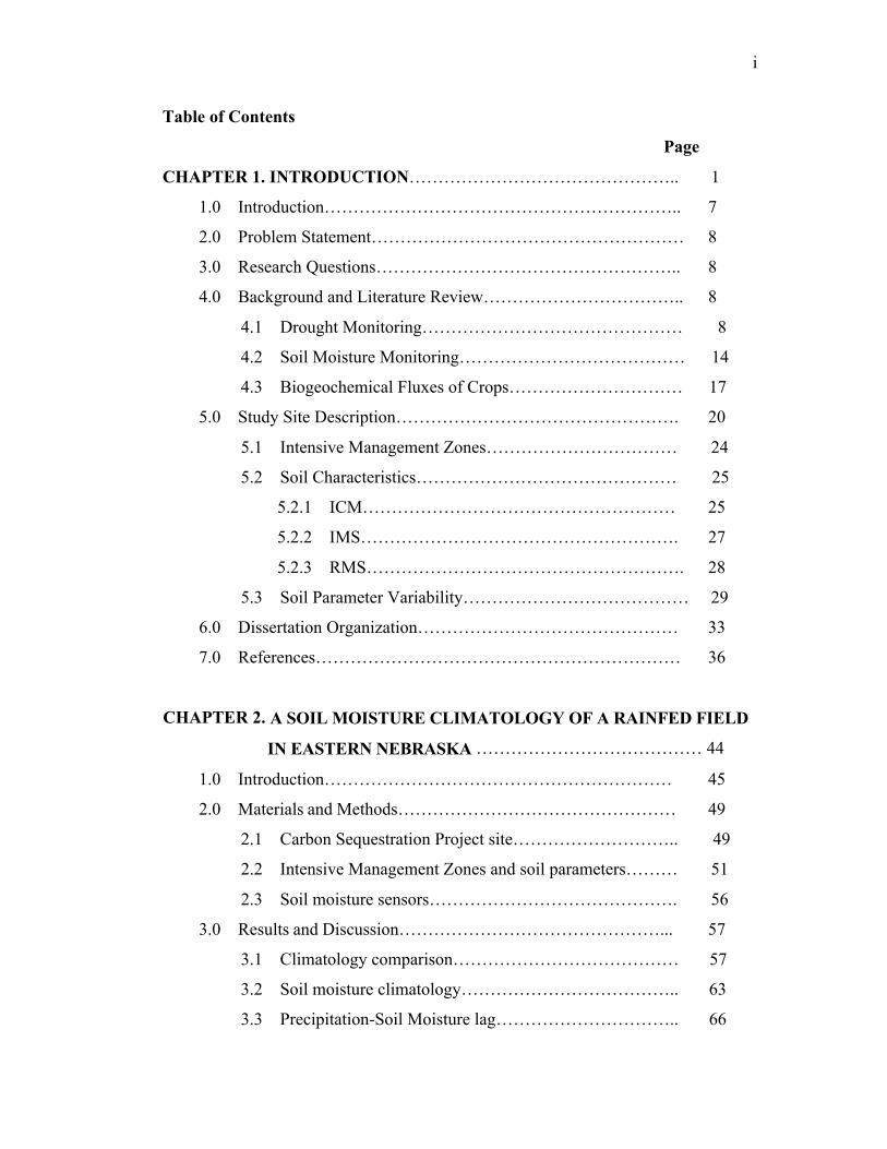
Table of Contents
Page
CHAPTER 1. INTRODUCTION……………………………………….. 1
1.0 Introduction…………………………………………………….. 7
2.0 Problem Statement……………………………………………… 8
3.0 Research Questions…………………………………………….. 8
4.0 Background and Literature Review…………………………….. 8
4.1 Drought Monitoring……………………………………… 8
4.2 Soil Moisture Monitoring………………………………… 14
4.3 Biogeochemical Fluxes of Crops………………………… 17
5.0 Study Site Description…………………………………………. 20
5.1 Intensive Management Zones…………………………… 24
5.2 Soil Characteristics……………………………………… 25
5.2.1 ICM……………………………………………… 25
5.2.2 IMS………………………………………………. 27
5.2.3 RMS………………………………………………. 28
5.3 Soil Parameter Variability………………………………… 29
6.0 Dissertation Organization……………………………………… 33
7.0 References……………………………………………………… 36
CHAPTER 2. A SOIL MOISTURE CLIMATOLOGY OF A RAINFED FIELD
IN EASTERN NEBRASKA ………………………………… 44
1.0 Introduction…………………………………………………… 45
2.0 Materials and Methods………………………………………… 49
2.1 Carbon Sequestration Project site……………………….. 49
2.2 Intensive Management Zones and soil parameters……… 51
2.3 Soil moisture sensors……………………………………. 56
3.0 Results and Discussion………………………………………... 57
3.1 Climatology comparison………………………………… 57
3.2 Soil moisture climatology……………………………….. 63
3.3 Precipitation-Soil Moisture lag………………………….. 66
ii
3.4 Precipitation-Soil Moisture paradox…………………….. 79
4.0 Summary and Conclusions……………………………………. 81
5.0 Acknowledgements……………………………………………. 85
6.0 References……………………………………………………… 85
CHAPTER 3. THE DYNAMIC RELATIONSHIP BETWEEN SOIL
MOISTURE AND BIOPHYSICAL
MEASUREMENTS……………………………………………………. 92
1.0 Introduction……………………………………………………. 93
2.0 Materials and Methods………………………………………… 95
2.1 Carbon Sequestration Project study site…………………. 95
2.2 Eddy covariance flux method and measurement………… 96
2.3 Soil moisture sensors…………………………………….. 97
2.4 Soil water calculations………………………………….. 98
2.5 Potential evapotranspiration calculations………………. 99
2.6 Development stages and period definitions……………... 100
3.0 Results and Discussion………………………………………… 101
3.1 Dry seasons……………………………………………… 101
3.2 Wet seasons……………………………………………… 114
4.0 Summary and Conclusions……………………………………. 124
5.0 Acknowledgements……………………………………………. 126
6.0 References……………………………………………………... 127
CHAPTER 4. MONITORING THE EFFECTS OF RAPID ONSET OF
DROUGHT ON NON-IRRIGATED MAIZE WITH
AGRONOMIC DATA AND CLIMATE-BASED DROUGHT
INDICES............................................................................. 130
1.0 Introduction…………………………………………………… 131
2.0 Materials and Methods………………………………………… 135
iii
2.1 Study site………………..……………………………….. 135
2.2 Eddy covariance flux method and measurement………… 137
2.3 Soil moisture sensors…………………………………….. 138
2.4 Soil water calculations…………………………………… 139
2.5 Development stages……………………………………… 140
2.6 Calculation of SPI and SPEI…………………………….. 140
3.0 Results and Discussion………………………………………… 143
3.1 Field management and weather conditions……………… 143
3.2 Moist phase……………………………………………… 154
3.3 Drying phase…………………………………………….. 158
3.4 Stressed phase…………………………………………… 164
3.5 Recharge phase………………………………………….. 169
4.0 Conclusions……………………………………………………. 171
5.0 Acknowledgements…………………………………………….. 173
6.0 References……………………………………………………… 174
CHAPTER 5. CONCLUSIONS………………………………………….. 182
iv
LIST OF TABLES
Chapter 1
Table 1. Soil parameters at ICM………………………………………… 26
Table 2. Soil parameters at IMS………………………………………… 28
Table 3. Soil parameters at RMS………………………………………… 29
Table 4a. Mean and standard deviation of two soil parameters (porosity
and the log of saturated hydraulic conductivity) obtained from
lab measurements for different soil textures at the three field
sites (ICM, IMS, RMS)………………………………………….. 30
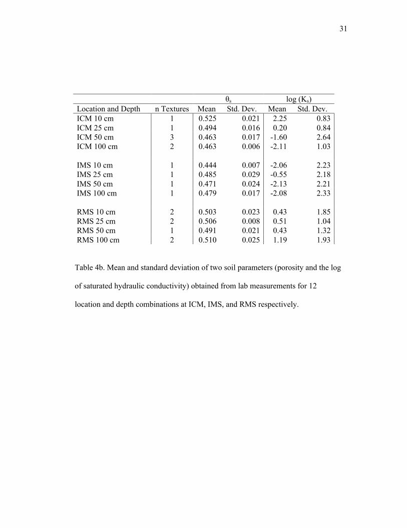
Table 4b. Mean and standard deviation of two soil parameters (porosity
and the log of saturated hydraulic conductivity) obtained from
lab measurements for 12 location and depth combinations at
ICM, IMS, and RMS respectively………………………………. 31
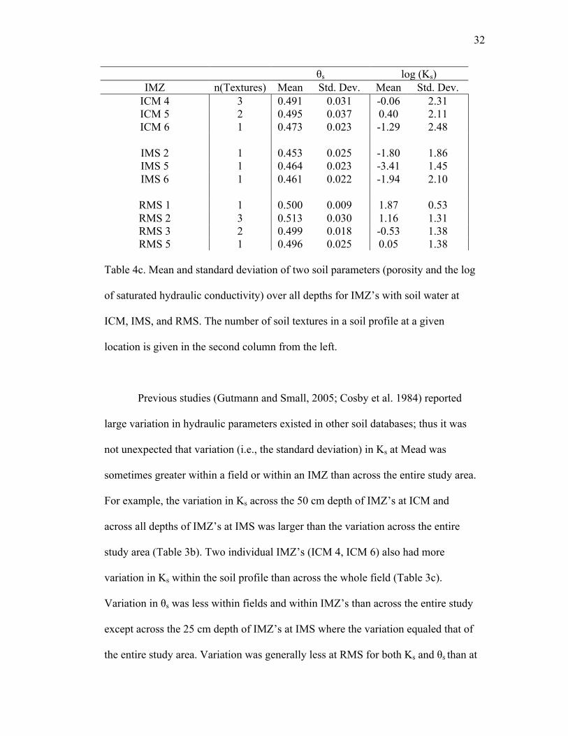
Table 4c. Mean and standard deviation of two soil parameters (porosity
and the log of saturated hydraulic conductivity) over all depths
for IMZ’S with soil water at ICM, IMS, and RMS…………….. 32
Chapter 2
Table 1. Crop management and final yield values for IMS and RMS……. 52
Table 2. Mean and standard deviation of two soil parameters (porosity
and the log of saturated hydraulic conductivity) obtained from
lab measurements for (a) 8 location and depth combinations, and
(b) over all depths at IMS and RMS…………………………… 54
v
Table 3. Median, minimum, maximum, and the 10th and 90th percentiles
of growing season precipitation (mm) during the 30-year period
(1982-2011) at all sites………………………………………….. 58
Table 4. Median, minimum, maximum July and August (JA)
precipitation (mm) during the 30-year period (1982-2011) at all
sites used for the climatology…………………………………… 60
Table 5. Median, minimum, and maximum number of days in a growing
season during the POR when maximum temperatures equaled or
exceeded 35°C…………………………………………………... 60
Table 6. Total RMS growing season precipitation, average RMS water
content at 10 cm, 25 cm, 50 cm, and 100 cm by season, and the
number of days in a season when the water content at 10 cm and
50 cm was such that it was less than 50 percent of available
water for the respective depth…………………………………… 64
Table 7. Correlation (R) between RMS averaged soil moisture and
precipitation over the previous 14 days, 30 days, and 60 days….. 68
Table 8. Total antecedent precipitation in the 14, 30, and 60 days prior to
1 July at Mead, NE in each season during the study period…….. 78
Table 9. Total growing season precipitation (mm) at RMS, the number of
irrigation treatments, and total irrigation amount applied (mm)
over the eight growing seasons at IMS………………………….. 80

vi
Chapter 3
Table 1. Crop management and final yield values for IMS and RMS……. 102
Table 2. Total precipitation (with irrigation at IMS), evapotranspiration
(mm), potential evapotranspiration (mm), and gross primary
productivity (g C m-2) at IMS and RMS over a 31-day period
ranging from 10-days prior to silking to 20 days following
silking……………………………………………………………. 103
vii
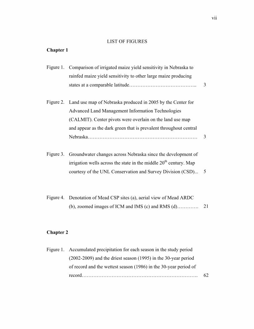
LIST OF FIGURES
Chapter 1
Figure 1. Comparison of irrigated maize yield sensitivity in Nebraska to
rainfed maize yield sensitivity to other large maize producing
states at a comparable latitude………………………………….. 3
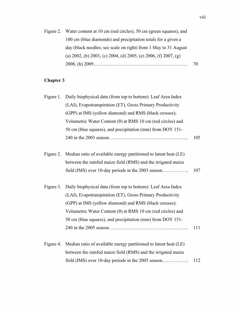
Figure 2. Land use map of Nebraska produced in 2005 by the Center for
Advanced Land Management Information Technologies
(CALMIT). Center pivots were overlain on the land use map
and appear as the dark green that is prevalent throughout central
Nebraska………………………………………………………… 3
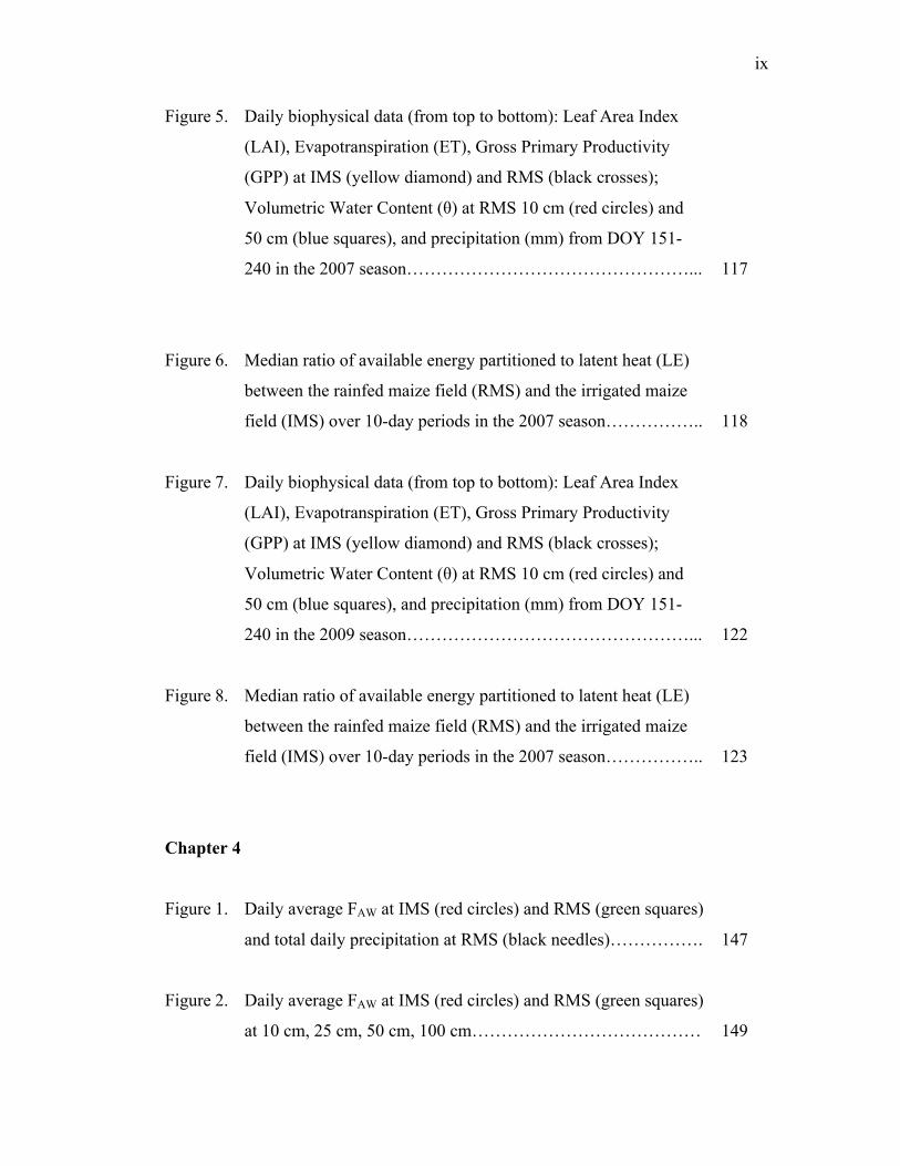
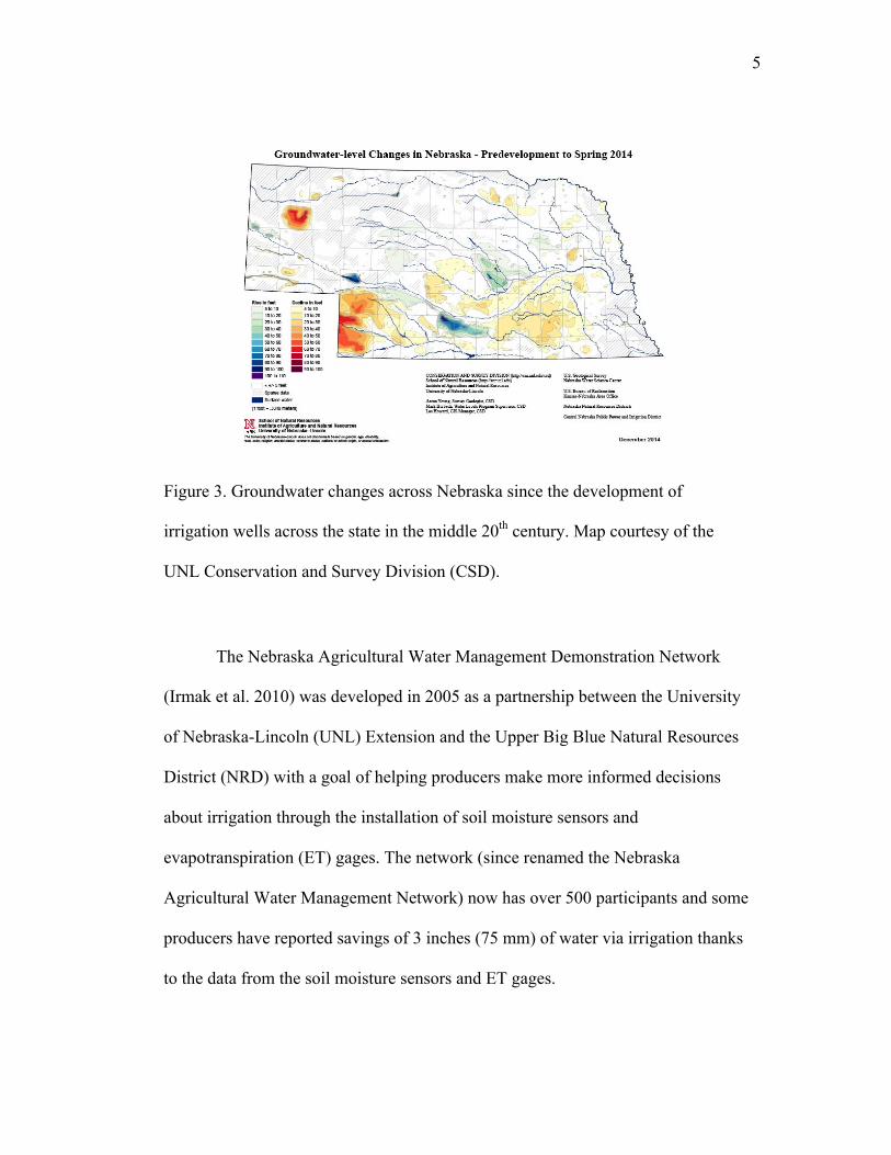
Figure 3. Groundwater changes across Nebraska since the development of
irrigation wells across the state in the middle 20th century. Map
courtesy of the UNL Conservation and Survey Division (CSD)... 5
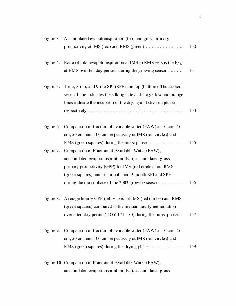
Figure 4. Denotation of Mead CSP sites (a), aerial view of Mead ARDC
(b), zoomed images of ICM and IMS (c) and RMS (d)…………. 21
Chapter 2
Figure 1. Accumulated precipitation for each season in the study period
(2002-2009) and the driest season (1995) in the 30-year period
of record and the wettest season (1986) in the 30-year period of
record……………………………………………………………. 62
viii
Figure 2. Water content at 10 cm (red circles), 50 cm (green squares), and
100 cm (blue diamonds) and precipitation totals for a given a
day (black needles; see scale on right) from 1 May to 31 August
(a) 2002, (b) 2003, (c) 2004, (d) 2005, (e) 2006, (f) 2007, (g)
2008, (h) 2009…………………………………………………… 70
Chapter 3
Figure 1. Daily biophysical data (from top to bottom): Leaf Area Index
(LAI), Evapotranspiration (ET), Gross Primary Productivity
(GPP) at IMS (yellow diamond) and RMS (black crosses);
Volumetric Water Content (θ) at RMS 10 cm (red circles) and
50 cm (blue squares), and precipitation (mm) from DOY 151-
240 in the 2003 season…………………………………………... 105
Figure 2. Median ratio of available energy partitioned to latent heat (LE)
between the rainfed maize field (RMS) and the irrigated maize
field (IMS) over 10-day periods in the 2003 season…………….. 107
Figure 3. Daily biophysical data (from top to bottom): Leaf Area Index
(LAI), Evapotranspiration (ET), Gross Primary Productivity
(GPP) at IMS (yellow diamond) and RMS (black crosses);
Volumetric Water Content (θ) at RMS 10 cm (red circles) and
50 cm (blue squares), and precipitation (mm) from DOY 151-
240 in the 2005 season…………………………………………... 111
Figure 4. Median ratio of available energy partitioned to latent heat (LE)
between the rainfed maize field (RMS) and the irrigated maize
field (IMS) over 10-day periods in the 2005 season…………….. 112
ix
Figure 5. Daily biophysical data (from top to bottom): Leaf Area Index
(LAI), Evapotranspiration (ET), Gross Primary Productivity
(GPP) at IMS (yellow diamond) and RMS (black crosses);
Volumetric Water Content (θ) at RMS 10 cm (red circles) and
50 cm (blue squares), and precipitation (mm) from DOY 151-
240 in the 2007 season…………………………………………... 117
Figure 6. Median ratio of available energy partitioned to latent heat (LE)
between the rainfed maize field (RMS) and the irrigated maize
field (IMS) over 10-day periods in the 2007 season…………….. 118
Figure 7. Daily biophysical data (from top to bottom): Leaf Area Index
(LAI), Evapotranspiration (ET), Gross Primary Productivity
(GPP) at IMS (yellow diamond) and RMS (black crosses);
Volumetric Water Content (θ) at RMS 10 cm (red circles) and
50 cm (blue squares), and precipitation (mm) from DOY 151-
240 in the 2009 season…………………………………………... 122
Figure 8. Median ratio of available energy partitioned to latent heat (LE)
between the rainfed maize field (RMS) and the irrigated maize
field (IMS) over 10-day periods in the 2007 season…………….. 123
Chapter 4
Figure 1. Daily average FAW at IMS (red circles) and RMS (green squares)
and total daily precipitation at RMS (black needles)……………. 147
Figure 2. Daily average FAW at IMS (red circles) and RMS (green squares)
at 10 cm, 25 cm, 50 cm, 100 cm………………………………… 149
x
Figure 3. Accumulated evapotranspiration (top) and gross primary
productivity at IMS (red) and RMS (green)…………………….. 150
Figure 4. Ratio of total evapotranspiration at IMS to RMS versus the FAW
at RMS over ten day periods during the growing season………. 151
Figure 5. 1-mo, 3-mo, and 9-mo SPI (SPEI) on top (bottom). The dashed
vertical line indicates the silking date and the yellow and orange
lines indicate the inception of the drying and stressed phases
respectively……………………………………………………… 153
Figure 6. Comparison of fraction of available water (FAW) at 10 cm, 25
cm, 50 cm, and 100 cm respectively at IMS (red circles) and
RMS (green squares) during the moist phase…………………… 155
Figure 7. Comparison of Fraction of Available Water (FAW),
accumulated evapotranspiration (ET), accumulated gross
primary productivity (GPP) for IMS (red circles) and RMS
(green squares), and a 1-month and 9-month SPI and SPEI
during the moist phase of the 2003 growing season……………. 156
Figure 8. Average hourly GPP (left y-axis) at IMS (red circles) and RMS
(green squares) compared to the median hourly net radiation
over a ten-day period (DOY 171-180) during the moist phase…. 157
Figure 9. Comparison of fraction of available water (FAW) at 10 cm, 25
cm, 50 cm, and 100 cm respectively at IMS (red circles) and
RMS (green squares) during the drying phase………………….. 159
Figure 10. Comparison of Fraction of Available Water (FAW),
accumulated evapotranspiration (ET), accumulated gross
xi
primary productivity (GPP) for IMS (red circles) and RMS
(green squares), and a 1-month and 9-month SPI and SPEI
during the drying phase of the 2003 growing season…………… 161
Figure 11. Average hourly GPP (left y-axis) at IMS (red circles) and RMS
(green squares) compared to the median hourly net radiation
over a ten-day period (DOY 171-180) during the drying phase… 163
Figure 12. Comparison of fraction of available water (FAW) at 10 cm, 25
cm, 50 cm, and 100 cm respectively at IMS (red circles) and
RMS (green squares) during the stressed phase………………… 165
Figure 13. Comparison of Fraction of Available Water (FAW),
accumulated evapotranspiration (ET), accumulated gross
primary productivity (GPP) for IMS (red circles) and RMS
(green squares), and a 1-month and 9-month SPI and SPEI
during the stressed phase of the 2003 growing season………… 167
Figure 14. Average hourly GPP (left y-axis) at IMS (red circles) and RMS
(green squares) compared to the median hourly net radiation
over a ten-day period (DOY 171-180) during the stressed phase.. 168
Figure 15. Comparison of fraction of available water (FAW) at 10 cm, 25
cm, 50 cm, and 100 cm respectively at IMS (red circles) and
RMS (green squares) during the recharge phase………………... 170
1
CHAPTER 1: INTRODUCTION
1.0 Introduction
Agricultural production, particularly of maize and soybeans, is a major
component of Nebraska’s economy and identity. However, agricultural production
in Nebraska faces increasing challenges, particularly in areas dependent on
irrigation. One of the larger concerns is the potential for excessive groundwater
depletion due to increased demand for food and fuel from Nebraska crops and
increasing risks of water stress in growing seasons due to climate change. Given
the importance of agricultural production to the state and the increasing
environmental risks, it has become essential for a deeper understanding of the soil-
plant-atmosphere continuum to help producers make more informed management
decisions. One of the variables that producers are starting to use for decision-
making is soil moisture. Soil moisture is an integral part of the hydrologic cycle
and an essential component in our understanding of land-atmosphere interactions.
Improved understanding of soil moisture response under major cash crops, such as
maize and soybeans, and insights into the dynamics of the soil moisture-crop-
atmosphere continuum are needed to help producers in irrigated regions make more
informed decisions.
Contrary to popular belief, Nebraska has diverse terrain and ecosystems,
ranging from predominant non-irrigated maize-soybean cropping systems in the far
eastern corner to the semi-arid landscape of irrigated cropland and pasture in the
western Panhandle. Precipitation gradients are sharp in the state and range from an
average of just under 900 mm in the far southeast to an average of 300 mm in the

2
western portion of the Nebraska. Thus, most areas in the far eastern corner of
Nebraska, as is the case in Iowa and other states to the east, can regularly receive
high-yielding crops under rainfed conditions, while crops grown west of the 100th
meridian require irrigation for crops to achieve high yields.
Irrigated agriculture has provided consistently high-yielding crops for
Nebraska producers and in a year when severe drought is affecting much of the
Corn Belt, this can help to ensure that there will still be a stable supply of grain
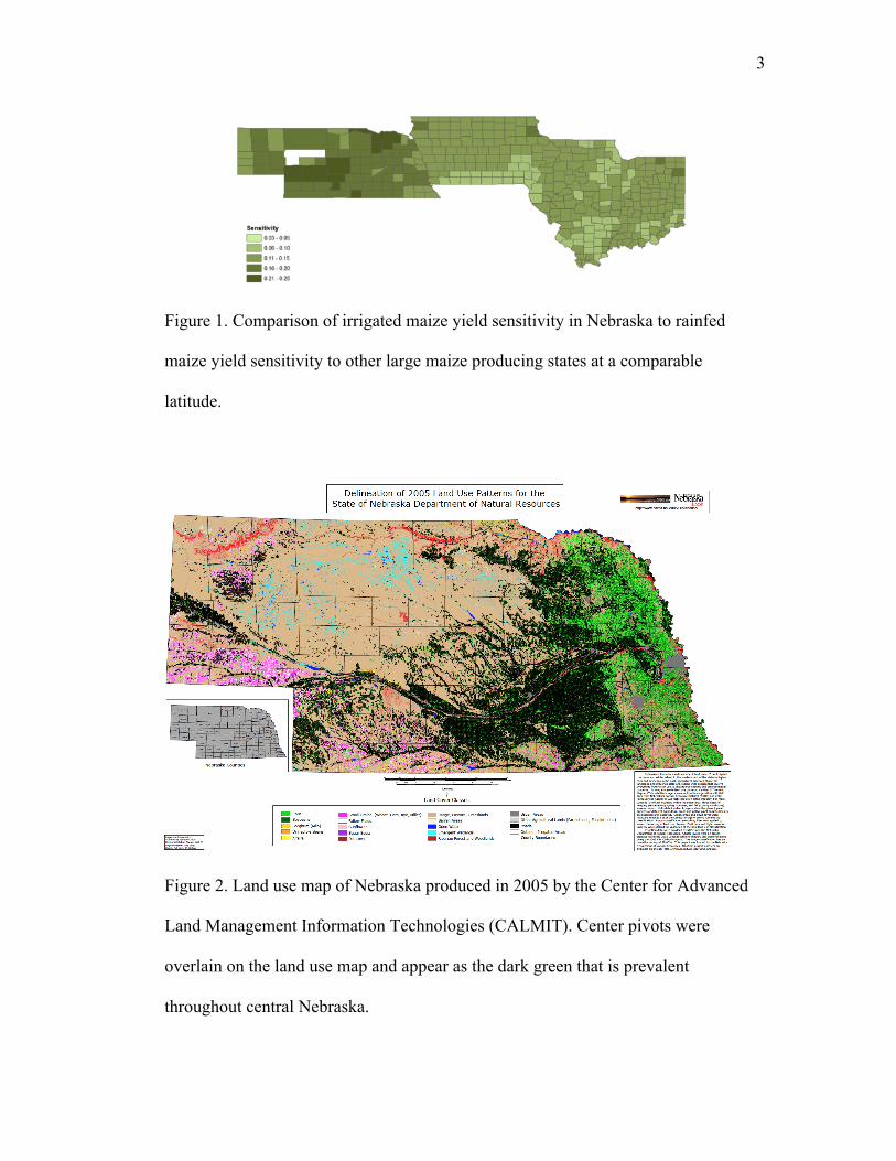
from the United States. One measure of how consistent irrigated maize yields have
been in Nebraska is with a sensitivity analysis, which in this case is defined as the
slope of the maize yield trend line from 1950-2009 divided by the root mean
square error over the same period. Figure 1 shows that irrigated yields in Nebraska
have a higher sensitivity (i.e., more consistent) than rainfed yields in states to the
east (Iowa, Illinois, and Indiana), particularly in central and western Nebraska
where almost all of the maize was irrigated according to a 2005 Land Use map
produced by the Center for Advanced Land Management Information
Technologies (CALMIT; Fig. 2) .
3
Figure 1. Comparison of irrigated maize yield sensitivity in Nebraska to rainfed
maize yield sensitivity to other large maize producing states at a comparable
latitude.
Figure 2. Land use map of Nebraska produced in 2005 by the Center for Advanced
Land Management Information Technologies (CALMIT). Center pivots were
overlain on the land use map and appear as the dark green that is prevalent
throughout central Nebraska.
4
The economic benefits of this irrigation are also significant, not just
because it results in more potential profit for producers, but also because these
profits are often invested in new-equipment and better technology that allow
producers to be more efficient. Local governments and schools also benefit from
irrigation as the higher value of land generates more revenues. Thus, irrigation is
the “life blood” of many areas of rural Nebraska, particularly west of Seward.
However, these tremendous benefits are not without costs or concerns. In
many areas of Nebraska, groundwater depletion has been significant over the past
several decades (Fig. 3) and irrigation restrictions were enforced in some areas of
the state after the last major drought in 2012. Judicious use of groundwater (and all
water) resources is therefore essential across the state (Bleed et al. 2015).
Thankfully there are efforts underway to help producers effectively schedule
irrigation treatments to minimize the over-depletion of groundwater
5
Figure 3. Groundwater changes across Nebraska since the development of
irrigation wells across the state in the middle 20th century. Map courtesy of the
UNL Conservation and Survey Division (CSD).
The Nebraska Agricultural Water Management Demonstration Network
(Irmak et al. 2010) was developed in 2005 as a partnership between the University
of Nebraska-Lincoln (UNL) Extension and the Upper Big Blue Natural Resources
District (NRD) with a goal of helping producers make more informed decisions
about irrigation through the installation of soil moisture sensors and
evapotranspiration (ET) gages. The network (since renamed the Nebraska
Agricultural Water Management Network) now has over 500 participants and some
producers have reported savings of 3 inches (75 mm) of water via irrigation thanks
to the data from the soil moisture sensors and ET gages.

6
The previous paragraph demonstrates how essential knowledge of soil
moisture and biophysical variables, such as ET, can be in helping inform producers
about irrigation decisions. Long-term field-scale averages of soil moisture and
biophysical data have been somewhat rare to date but a significant void in this area
was filled with the establishment of the ongoing UNL Carbon Sequestration
Project (CSP) in 2001 at the University of Nebraska-Lincoln Mead Agricultural
Research and Development Center (ARDC) near the towns of Ithaca and Mead,
NE.
The ARDC is located in east-central Nebraska and is situated about 35
kilometers to the north-northeast of Lincoln and about 25 kilometers to the west-
southwest of Omaha, the state’s largest city. Its location in east-central Nebraska
puts it at the western edge of what is commonly referred to as the U.S. (dryland)
Corn Belt and just to the east of one of the most heavily irrigated places in the U.S.
(Johnson et al. 2011). It is at this site where my dissertation research has been
focused.
As mentioned earlier, the CSP is still ongoing today but the study period for
this research was an eight-year period from 2002 to 2009. This period was chosen
because it represented a period of consistent maize-soybean rotations and
management practices at the two fields used in analysis and because of the
diversity of the agro-climatological conditions experienced during that time. The
two fields used for analysis in the dissertation, consisted of a field with an
irrigated, maize-soybean rotation (IMS) and a field with a rainfed, maize-soybean
rotation (RMS). These two field sites were chosen because of the same crop was
7
grown in both field during each of the study period (i.e., the crop rotation was
identical) and because management practices were consistent during that time. The
study period chosen had conditions that ranged from unusually moist to average to
excessively dry when compared to the 30-year period of record at Mead.
Temperatures were slightly above the 1 May-30 September average of 20.6°C in
four of the seven seasons, though only 2002 was more than 1.0°C above that
average, and slightly below that average in two others. Only 2009 was more than
1.0°C below the 30-year average. Additional information on the sites is contained
in section 1.5 of this chapter.
2.0 Problem Statement
Soil moisture is an integral part of the hydrologic cycle and an essential
component in our understanding of land-atmosphere interactions. Agriculture
production, particularly of maize and soybeans, are a major component of
Nebraska’s economy and identity. Even with increased use efficient center-pivot
irrigation technology and improved genetics for drought tolerance, producers are
still vulnerable to major droughts and are often under legal obligations to only use
a certain amount of water per season for irrigating crops. It therefore is as
important as ever to understand the link between precipitation, soil moisture, and
crop stress for decisions about when and how much to irrigate. The goal of the
dissertation is to demonstrate the link between soil moisture and other biophysical
variables, such as ET and GPP, over an eight-year period that included abnormally
wet and dry conditions from a study site that is uniquely situated in a transition

8
zone from the semi-arid High Plains to the west and the sub-humid Corn Belt to the
east.
3.0 Research Questions
1) How does soil water in a rainfed field located in an agro-climatological
transition zone vary within and between growing seasons and how does it
compare to a nearby irrigated field during anomalously wet and dry
periods?
2) How does soil water relate to biophysical variables, such as
evapotranspiration and gross primary productivity, and the surface
energy budget at both a rainfed and irrigated maize field in wet and dry
seasons?
3) How did soil water and biophysical variables compare to short-term and
long-term drought indices during a flash drought in the 2003 growing
season?
4.0 Background and Literature Review
4.1 Drought Monitoring
During parts of the study period, drought conditions were prevalent at
Mead and throughout the state and surrounding region. Drought is a natural,
recurring phenomena that occurs everywhere at various points in time and is
occurring somewhere on Earth at any given point of time. Drought is a complex
topic with ecosystem impacts that vary with its intensity and duration and socio-
economic impacts that often magnify problems for agricultural producers and the
9
most vulnerable members of society. Perhaps the most telling factor for the true
complexity of drought is the lack of a true universal definition and is often
considered in four broad categories defined by Wilhite and Glantz (1985):
meteorological, agricultural, hydrological, and socioeconomic.
Meteorological drought is typically referred to as some deficit of
precipitation from normal over a period of time. Agricultural drought refers to loss
or decline of soil moisture, groundwater, and irrigation sources, such as
streamflows, that lead to reductions in crop yield, forage quality, and water for
livestock. Hydrological drought refers to declines in streamflows, lake levels, and
reservoir levels from a prolonged period of precipitation deficits. An increased
frequency of irrigation treatments can help offset agricultural impacts during
drought but it can exacerbate hydrological impacts as a consequence. Socio-
economic drought broadly refers to inter-linked societal and economic impacts that
result from the three aforementioned drought categories. Socio-economic impacts
can be the most severe and longest lasting in duration but are often difficult to
quantify and/or separate from other factors.
Even though drought is often viewed within the four categories, there is
often significant overlap and linkages amongst them. Meteorological drought, or a
deficit of precipitation, can be viewed as the foundation for the other three
categories of drought. In other words, meteorological drought can be mutually
exclusive and independent of the other categories but agricultural, hydrological,
and socioeconomic droughts are dependent on a deficit of precipitation. While all
10
aspects of drought are important, the primary drought focus in this dissertation will
be on agricultural drought.
Drought has often been quantified with climate-based drought indices. One
of the first was the Palmer Drought Severity Index (PDSI), which was developed
by Palmer (1965) to achieve an objective of “developing a general methodology
for evaluating drought in terms of an index that permits time and space
comparisons of drought severity." The PDSI is calculated from a simple water
balance model that uses five factors: precipitation, potential evapotranspiration
(Thornthwaite 1948), recharge, runoff, and soil moisture loss to determine whether
recent precipitation was sufficient to maintain a normal water balance.
The PDSI is divided into 11 categories ranging from extreme drought to
extreme wet spell (Heim 2002). Empirical constants for climate characteristic and
duration factors used in the calculation were derived from data across nine
locations in seven U.S. states. This has been a source of criticism for the PDSI as
its performance has often failed to reflect differences in climate regimes,
particularly in the western U.S. (Alley 1984; Guttman et al. 1992; Guttman 1997;
Heim 2002; Wells et al. 2004). Some of the issues with the PDSI were resolved
with the development of the Self-Calibrating Palmer Drought Severity Index (SC-
PDSI). Wells et al. (2004) replaced the empirical constants of the PDSI with
dynamic and location specific values and the SC-PDSI showed lower frequencies
of extreme wet and drought conditions than the PDSI when tested at several
locations in the U.S. Great Plains. Thus, the SC-PDSI represents more realistic
variability and frequency of extreme events than the PDSI.
11
Mavromatis (2007) found that the SC-PDSI explained 92 percent of wheat
variability in southern Greece. Dubrovsky et al. (2009) further found that the SC-
PDSI exhibited a wider spectrum of drought conditions across the Czech Republic
than the SPI due to its inclusion of temperature. However, like the PDSI, the SC-
PDSI still has a fixed temporal scale and an autoregressive characteristic that
allows for the index to be affected by conditions up to four years prior (Guttman
1998). These and other issues with the PDSI led to the development of normalized
drought indices over the past twenty years.
McKee et al. (1993) developed the Standardized Precipitation Index (SPI)
in response to demand from Colorado decision makers for an index that expressed
current conditions in terms of water supply, deficit, and probability. Since
precipitation is generally not normally distributed, a transformation was applied to
the probability of observed precipitation for a set time period. A 3-parameter
Pearson-Type III distribution was found to be the best universal model for
calculation of the SPI (Guttman 1999). A thorough description of the SPI
calculation is contained in Lloyd-Hughes and Saunders (2002). The SPI has the
advantage of being spatially invariant and an indicator of drought on multiple time
scales (Guttman 1999), though caution has been advised when comparing the SPI
between sites with very different periods of record and at short time scales during
distinct dry seasons (Wu et al. 2005).
The SPI has been widely used for operational and research purposes. Hayes
et al. (1999) showed that the SPI detected drought conditions a full month ahead of
the PDSI during the U.S. southern plains drought of 1996. Livida and
12
Assimakopoulos (2004) used the SPI to show that mild and moderate drought were
more common on the three- and six- month time scale across northern Greece
while severe drought was more frequent across southern Greece. Brown et al.
(2008) integrated the SPI with satellite derived vegetation metrics and biophysical
data to produce 1-km maps of the Vegetation Drought Response Index (VegDRI).
McRoberts and Nielsen-Gammon (2012) used daily precipitation from the
Advanced Hydrologic Prediction Service multisensor precipitation estimates
(MPE) and Cooperative Observer Program (COOP) station data to obtain a high
resolution SPI to be used for guidance for the U.S. Drought Monitor (Svoboda et
al. 2002).
One criticism of a precipitation-only index like the SPI is that it does not
account for temperature effects on drought. For example, Hu and Wilson (2000)
showed that the PDSI was equally affected by large anomalies of temperature and
precipitation in the central United States. Vicente-Serrano et al. (2010) addressed
this issue with the development of the Standardized Precipitation Evaporation
Index (SPEI). The SPEI is calculated with the same procedure as the SPI as it
based on the monthly (or weekly) difference between precipitation and potential
evapotranspiration (ETp), using the ETp method from Thornthwaite (1948). The
Thornthwaite method of ETp was chosen over more robust methods, such as
Penman-Monteith (Monteith 1964), due to the simplicity of its calculation and its
reasonable performance when calculating a drought index, such as the PDSI
(Mavromatis 2007).
13
The incorporation of temperature into the SPEI also makes it more sensitive
to increased frequency and severity of droughts. For example, McEvoy et al.
(2011) found that the SPEI was an improvement over the SPI at identifying longer
durations of severe drought in Nevada and eastern California. Potop and Mozny
(2011) found that the SPEI depicted increasing drought severity in the Czech
Republic over the past few decades with warming temperatures. Thus, the SPEI is
an adequate index at assessing the impact of climate change (Begueria-Portugues et
al. 2010).
The development of drought indices allows for useful comparison of
conditions between locations and over long periods of time. However, caution
should still be applied when applying an index to long time-series of climate data.
Inhomogeneities in data from station relocations, instrumentation changes, and
growth of vegetation and urban boundaries do exist and analyses can be erroneous
if these items are not accounted for (Peterson et al. 1998). Nevertheless, climate-
based drought indices are useful at identifying the severity and duration of drought.
When considering agricultural drought, the emphasis is often on impacts
that occur over a shorter period of time (e.g., over part of a growing season). Short-
term droughts, commonly referred to as “flash” droughts, can occur within a longer
period of normal or above normal precipitation and bring devastating agricultural
impacts. For example, although precipitation was above normal in most of
Oklahoma during 1998, an intense, flash drought during the summer decimated the
state’s cotton and peanut crop (Basara et al 1998; Arndt and Johnson 2002). In
14
recent years, flash drought has increasingly been quantified by specialized metrics
and indices developed from climate and remotely sensed data.
For example, Otkin et al. (2014) developed a Rapid Change Index (RCI)
that identifies areas undergoing rapid moisture stress depicted by the Evaporative
Stress Index (ESI; Anderson et al. 2013) generated by the Atmosphere-Land
Exchange Inverse (ALEXI) surface energy balance model (Anderson et al. 1997,
Anderson et al. 2007b). Otkin et al. (2015) then applied a simple statistical method
to the RCI to determine if further intensification of flash drought was likely. While
these aforementioned studies were focused more on determining water stress from
flash drought from thermal band imagery, soil moisture was considered a very
important factor in all of them.
4.2 Soil Moisture Monitoring
Soil moisture may be one of the best indicators of flash drought if there are
previous years of data to compare against, as shown with a soil moisture index
(SMI) developed by Hunt et al. (2009). However, longer-term in-situ soil moisture
data from under crop cover that could further validate metrics like the RCI or help
to improve our understanding of the soil-plant-atmosphere relationship in times of
drought stress have been somewhat rare to this point. Thus, one of the primary
goals of this dissertation is to increase our understanding of the relationship
between soil moisture and biophysical indicators of crop moisture stress (e.g.,
reduced ET) on a true field scale during shorter dry spells and during a true flash
drought.
15
Soil moisture is an integral part of the Earth’s hydrologic cycle. The
standard soil water balance equation is given as follows by Hillel (2004) in
Equation 1.1:
dS/dt = P – ET – R – Dr (1.1)
where δS/δt, P, ET, R, Dr are the change in soil water, precipitation,
evapotranspiration, runoff, and drainage over a time period t. Soil water movement
into soils is based on the conservation mass. Thus, the rate of infiltration into a soil
must be equaled by a change in water content (Eq. 1.2):
𝜕𝜃/𝜕𝑡 = −𝜕𝑞/𝜕𝑧
(1.2)
Soil moisture flow in unsaturated soils is based on Darcy’s Law (Eq. 1.3),
which essentially states that the flow into a soil is proportional to the hydraulic
gradient:
𝑞 = −𝐾 𝜕𝐻/𝜕𝑧
(1.3)
where q is the flux of water, K is the hydraulic conductivity (mm s-1), and !!!!
is the
hydraulic gradient (mm). However, during periods of successive wetting and
drying phases, soils often have high levels of hysteresis. This issue is solved using
by combining the principles of the conservation of mass from Eq. 1 and Darcy’s
Law in Eq. 2 to obtain the Richards equation (Eq. 2.4).
𝜕𝜃𝜕𝑡 =
𝜕𝜕𝑧 𝐾
𝜕(𝑧 + 𝜓)𝜕𝑧
(1.4)
16
Since the flow is driven by the pressure of overlying water (z) and the
suction of capillary action drawing water down (ψ), we write the hydraulic gradient
in the Richards equation as H = z + ψ. Assuming that !"!"
=1, !"!"= !"
!"∙ !"!"
, and
𝐾 ∙ !"!"
is the soil water diffusivity (i.e., the combination of conductivity and
capillary pressure), we obtain a modified form of Richards equation (Eq. 1.5):
𝜕𝜃𝜕𝑡 =
𝜕𝜕𝑧 𝐾 + 𝐷
𝜕𝜃𝜕𝑧
(1.5)
The Richards equation is often simplified into the Green and Ampt
infiltration equation, which assumes a solid wetting front that proceeds downward
at a constant rate with constant matric (ψ) suction. Thus, the wetting front is
considered to be a plane that separates a uniformly infiltrated zone with a zone
with no infiltration. Infiltration (Eq.1.6) is then considered to be the product of the
depth of the wetting front (Lf) and θ.
𝐼 = 𝐿𝑓 ∙ ∆𝜃
(1.6)
The rate of advance of the wetting front is inversely proportional to the
cumulative infiltration and assuming that the rate of infiltration is equal to the
product of hydraulic conductivity and the change in pressure head over the wetting
front, we obtain Eq. 1.7
∆𝜃𝑑𝐿𝑓𝑑𝑡 = 𝐾
∆𝐻!𝐿𝑓
(1.7)
17
After further manipulation (see Hillel 2004 for further details) and
assuming time is large, the Green and Ampt approach simplifies to a delta function
approximation (Eq. 1.8) such that δ can assumed to be a constant.
𝐼 ~ 𝐾𝑡 + 𝛿
(1.8)
Thus, over a period of time after precipitation, the amount of infiltration
can be approximated to be the product hydraulic conductivity and time plus a
constant. Even though soil water infiltration is not discussed in great technical
detail in this dissertation, it was important to show (via the past several equations)
that hydraulic conductivity is a critical parameter in soil water infiltration. Exact
measures of hydraulic conductivity cannot be inferred in the CSP fields; however,
other laboratory measurements allowed for calculation of saturated hydraulic
conductivity via pedotransfer functions in Saxton and Rawls (2006). Thus the
ability of soils to infiltrate precipitation can be inferred at different areas within the
CSP fields. This is discussed further in section 1.5.
4.3 Biogeochemical Fluxes of Crops
Since its inception in 2001, the CSP has collected a wealth of flux
(carbon and energy) observations. These data are renowned enough to be used for
validation in irrigation modeling simulations at NASA Goddard Space Flight
Center (Lawston et al. in press) and for test cases in the Joint UK Land
Environment Simulator (JULES) model (Best et al. 2011). There is currently a goal
of making the Mead ARDC a testbed site for instrument calibration and validation
of land surface model output (UNL Newsroom 2014). Thus, the data used in the
18
dissertation are likely to be more in demand in the future due to increased
exposure.
Several works have been published, particularly in the realm of energy and
carbon balance. In Suyker et al. (2004), the authors presented results of net
ecosystem CO2 exhange (NEE) and gross primary productivity (GPP) during the
first year (2001) of the CSP. A dry and hot spell in the middle of that growing
season reduced leaf area index (LAI) and NEE at the rainfed maize soybean
rotation (RMS) compared to the irrigated maize soybean rotation (IMS).
Verma et al. (2005) wrote a detailed report on carbon exchange at all three
CSP fields during the first four seasons (2001-2004) of the project. They reported
that GPP was almost twice as high in a maize season as in a soybean season and
that net ecosystem production (NEP) was about the same in the rainfed and
irrigated field, as increased respiration in irrigated fields with higher soil moisture
offset the higher GPP at the irrigated sites compared to RMS.
Suyker and Verma (2009) presented detailed results from six years (2001-
2006) of evapotranspiraton (ET) data at ICM, IMS, and RMS. Growing season ET
accounted for an average of 84 and 72 percent of the annual evaporation at the
irrigated sites (ICM, IMS) and RMS respectively. As expected, annual ET was
higher at the irrigated sites than at RMS, particularly during the flash drought that
occurred during the 2003-2004 season, and was higher in maize years than in
soybean years at both IMS and RMS. The authors also showed that the crop
coefficient (Kc), which is calculated as the ratio of ET to reference ET (ETo), was
19
as much as 30 percent higher at IMS than at RMS during the middle of the 2003
flash drought.
A similar study with GPP over the 2001-2006 growing seasons sites
showed that the seasonal distributions of GPP were consistent in maize and
soybeans throughout the six seasons and that GPP was consistently higher in the
irrigated fields than at RMS (Suyker and Verma, 2010). This was especially true in
the 2003 growing season when cumulative GPP was reduced by 24 percent at RMS
compared to IMS. The authors also showed that there was no statistical difference
in the ET/ETo-LAI relationship compared to that of GPP-LAI.
In Suyker and Verma (2012), the authors showed that green leaf LAI was a
dominant factor in explaining interannual variability of GPP in maize, whereas
both LAI and photosynthetically active radiation (PAR) were dominat factors for
soybeans. As also shown in earlier results, mean annual GPP of soybeans was
significantly less than that of maize. However, in this paper the authors presented
results of how much of the GPP was eventually lost to respiration. In a maize year,
nearly 70 percent of accumulated GPP in maize was lost to respiration. This seems
like a lot until one considers that almost all of the accumulated GPP in the soybean
years was lost to respiration. Thus, both RMS and IMS were approximately carbon
neutral over several seasons, with IMS being a slight carbon source in the early
years due to enhanced respiration rates compared to the drier RMS.
20
5.0 Study Site Description
The CSP is located at the University of Nebraska-Lincoln (UNL)
Agricultural Research and Development Center in east-central Nebraska near the
towns of Ithaca and Mead, NE. The CSP is located in the north central United
States (Fig. 4a) and is roughly 45 km to the northeast of downtown of Lincoln,
Nebraska and 43 km to the west-southwest of downtown Omaha, Nebraska. The
CSP consists of three sites. The first agroecosystem is an irrigated, continuous
maize (ICM) site centered at 41˚09’54.2” N, 96˚ 28’35.9” W with an irrigated area
of 48.7 ha. The second agroecosystem is an irrigated, rotated maize-soybean (IMS)
site centered at 41˚09’53.5” N, 96˚ 28’12.3” W with an irrigated area of 52.4 ha.
Both ICM and IMS were irrigated rotations of maize and soybeans under no-till in
the ten years prior to the initialization of the CSP. The third agroecosystem is a
rainfed, rotated maize-soybean (RMS) site centered at 41˚10’46.8” N, 96˚ 26’22.7”
W with an area of 65.4 ha. Prior to the CSP, RMS had 2-4 ha plots of maize,
soybeans, wheat, and oats with tillage (Verma et al. 2005).
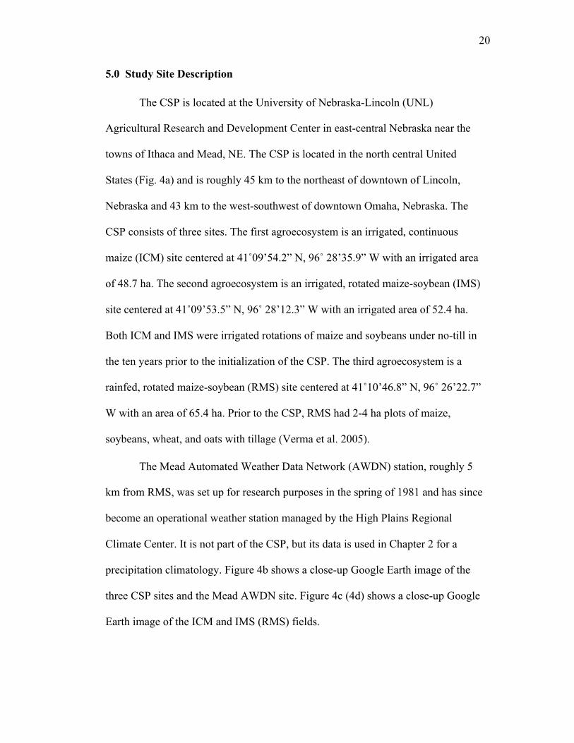
The Mead Automated Weather Data Network (AWDN) station, roughly 5
km from RMS, was set up for research purposes in the spring of 1981 and has since
become an operational weather station managed by the High Plains Regional
Climate Center. It is not part of the CSP, but its data is used in Chapter 2 for a
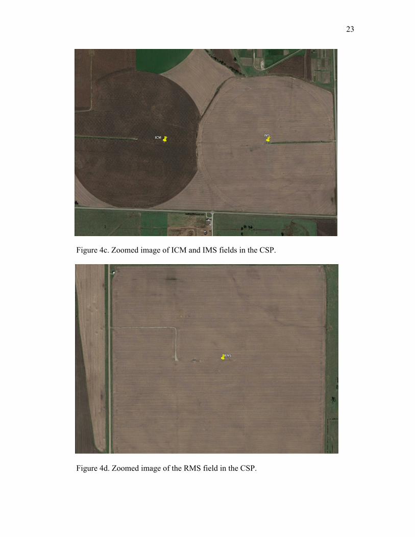
precipitation climatology. Figure 4b shows a close-up Google Earth image of the
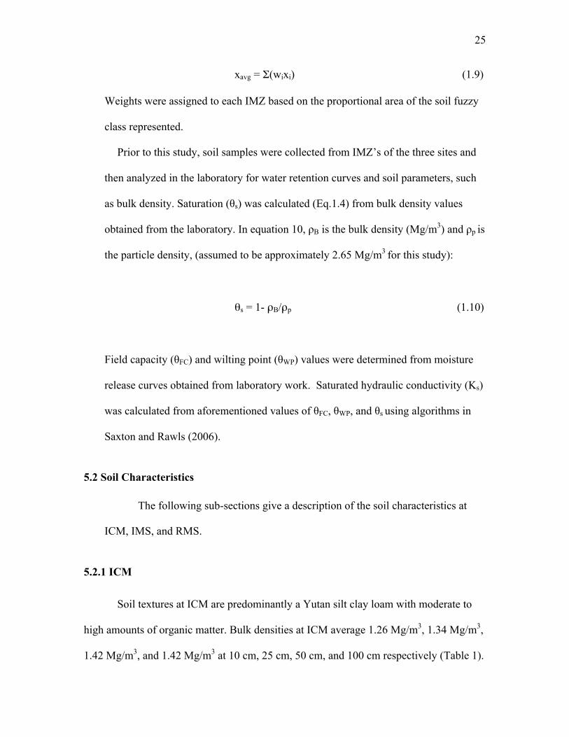
three CSP sites and the Mead AWDN site. Figure 4c (4d) shows a close-up Google
Earth image of the ICM and IMS (RMS) fields.
21
Figure 4a. The location of the CSP sites and the Mead AWDN site in relation to the
rest of the continental United States.
22
Figure 4b. Aerial view of the UNL Mead ARDC. Pins denote the middle of the
irrigated continuous maize (ICM) irrigated rotated maize-soybean (IMS) and rainfed
rotated maize-soybean (RMS) fields of the Carbon Sequestration Project and the
Mead AWDN site that has been operating since 1981.
23
Figure 4c. Zoomed image of ICM and IMS fields in the CSP.
Figure 4d. Zoomed image of the RMS field in the CSP.
24
5.1 Intensive Management Zones
Each CSP site consists of six, 20 m x 20 m intensive management zones,
hereafter referred to as IMZ’s, where detailed process-level studies of soil water,
soil carbon dynamics, canopy and soil gas exchange, crop growth and biomass
partitioning are established. Prior to the onset of the CSP in 2001, all three sites
were uniformly tilled by disking the top 10 cm to incorporate Phosphorous (P) and
Potassium (K) fertilizers and to homogenize the soil layer (Suyker and Verma,
2009). Nitrogen (N) fertilizer applications were applied to IMS and RMS prior to
planting in 2003; subsequent N applications were applied in June at IMS through
the center-pivot system in a process known as fertigation.
The IMZ locations were selected using k-means clustering applied to six
layers of environmental site information for 4 m x 4 m cells based broadly on soil
type, topography, and crop production potential across each site. Fine-scale spatial
information used for each site included a digital soil map, a digital elevation model,
a Veris map of soil electrical conductivity (0-30 cm), near infrared reflectance of
bare soil from the IKONOS satellite (4 km resolution), and a map of soil organic
matter (0-20 cm). Interpolation onto a 4 x 4 m grid was done by kriging. The
footprints of the IMZ’s are not equal in area and thus field-averaged calculations of
soil water are weighted using Equation 1.9 below, where wi is the weight (i.e.,
fraction of the field represented by the fuzzy classes associated with the i’th IMZ), x
is the measured soil water in the i’th IMZ and i increases from 1 to n (the total
number of IMZs per field):
25
xavg = Σ(wixi) (1.9)
Weights were assigned to each IMZ based on the proportional area of the soil fuzzy
class represented.
Prior to this study, soil samples were collected from IMZ’s of the three sites and
then analyzed in the laboratory for water retention curves and soil parameters, such
as bulk density. Saturation (θs) was calculated (Eq.1.4) from bulk density values
obtained from the laboratory. In equation 10, ρB is the bulk density (Mg/m3) and ρp is
the particle density, (assumed to be approximately 2.65 Mg/m3 for this study):
θs = 1- ρB/ρp (1.10)
Field capacity (θFC) and wilting point (θWP) values were determined from moisture
release curves obtained from laboratory work. Saturated hydraulic conductivity (Ks)
was calculated from aforementioned values of θFC, θWP, and θs using algorithms in
Saxton and Rawls (2006).
5.2 Soil Characteristics
The following sub-sections give a description of the soil characteristics at
ICM, IMS, and RMS.
5.2.1 ICM
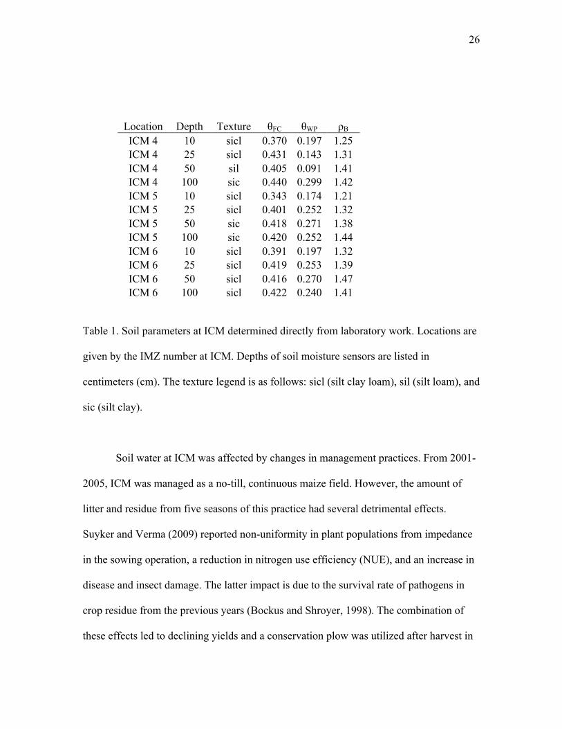
Soil textures at ICM are predominantly a Yutan silt clay loam with moderate to
high amounts of organic matter. Bulk densities at ICM average 1.26 Mg/m3, 1.34 Mg/m3,
1.42 Mg/m3, and 1.42 Mg/m3 at 10 cm, 25 cm, 50 cm, and 100 cm respectively (Table 1).
26
Location Depth Texture θFC θWP ρB ICM 4 10 sicl 0.370 0.197 1.25 ICM 4 25 sicl 0.431 0.143 1.31 ICM 4 50 sil 0.405 0.091 1.41 ICM 4 100 sic 0.440 0.299 1.42 ICM 5 10 sicl 0.343 0.174 1.21 ICM 5 25 sicl 0.401 0.252 1.32 ICM 5 50 sic 0.418 0.271 1.38 ICM 5 100 sic 0.420 0.252 1.44 ICM 6 10 sicl 0.391 0.197 1.32 ICM 6 25 sicl 0.419 0.253 1.39 ICM 6 50 sicl 0.416 0.270 1.47 ICM 6 100 sicl 0.422 0.240 1.41
Table 1. Soil parameters at ICM determined directly from laboratory work. Locations are
given by the IMZ number at ICM. Depths of soil moisture sensors are listed in
centimeters (cm). The texture legend is as follows: sicl (silt clay loam), sil (silt loam), and
sic (silt clay).
Soil water at ICM was affected by changes in management practices. From 2001-
2005, ICM was managed as a no-till, continuous maize field. However, the amount of
litter and residue from five seasons of this practice had several detrimental effects.
Suyker and Verma (2009) reported non-uniformity in plant populations from impedance
in the sowing operation, a reduction in nitrogen use efficiency (NUE), and an increase in
disease and insect damage. The latter impact is due to the survival rate of pathogens in
crop residue from the previous years (Bockus and Shroyer, 1998). The combination of
these effects led to declining yields and a conservation plow was utilized after harvest in
27
the fall of 2005 and every successive harvest thereafter. The conservation plow was
chosen over other standard tillage equipment because it minimizes soil disturbance and
vertically distributes around 2/3 of the residue within the top 25 cm of the soil, leaving
the remaining 1/3 on the soil surface.
Even though care was taken to avoid significant soil disturbances, the
conservation plow was used while the field was still a bit wet, which led to compaction
and an increase in bulk density at ICM. The effect of tillage at ICM was not consistent
across IMZ’s and was most significant in 2006. The effect of conservation tillage was
less pronounced in years after 2006 and the average water content (θ) at ICM 4 and ICM
5 was back around 2002-2005 levels by the 2007-2009 seasons. However, given the field
management differences at ICM within the study period, and the field management and
cropping differences between ICM and the two rotated sites, IMS and RMS, it was
decided to exclude ICM from analysis throughout the remainder of the dissertation. That
is not to imply that valuable data don’t exist from ICM; many papers have been published
with the data from ICM. Rather the focus and scope of the dissertation is more strongly
tied to direct comparisons of soil water and biophysical measurements between a
common crop at a rainfed and irrigated site (i.e., between RMS and IMS).
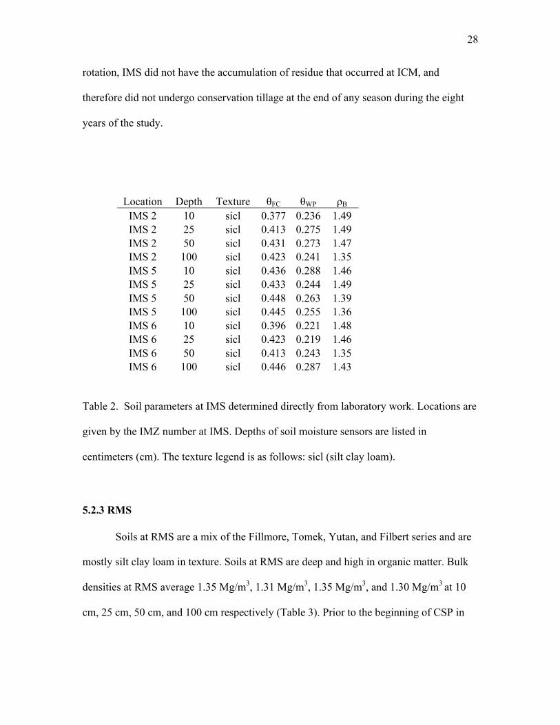
5.2.2 IMS Soils at IMS are a mix of the Yutan, Tomek, and Filbert series with silt clay loam
as the dominant soil texture. Bulk densities at IMS average 1.48 Mg/m3, 1.48 Mg/m3,
1.40 Mg/m3, and 1.38 Mg/m3 at 10 cm, 25 cm, 50 cm, and 100 cm respectively (Table 2).
Organic matter was high at all three IMZ’s with soil water measurements and IMS was
consistently the highest yielding field in the CSP. With a consistent maize-soybean
28
rotation, IMS did not have the accumulation of residue that occurred at ICM, and
therefore did not undergo conservation tillage at the end of any season during the eight
years of the study.
Location Depth Texture θFC θWP ρB IMS 2 10 sicl 0.377 0.236 1.49 IMS 2 25 sicl 0.413 0.275 1.49 IMS 2 50 sicl 0.431 0.273 1.47 IMS 2 100 sicl 0.423 0.241 1.35 IMS 5 10 sicl 0.436 0.288 1.46 IMS 5 25 sicl 0.433 0.244 1.49 IMS 5 50 sicl 0.448 0.263 1.39 IMS 5 100 sicl 0.445 0.255 1.36 IMS 6 10 sicl 0.396 0.221 1.48 IMS 6 25 sicl 0.423 0.219 1.46 IMS 6 50 sicl 0.413 0.243 1.35 IMS 6 100 sicl 0.446 0.287 1.43
Table 2. Soil parameters at IMS determined directly from laboratory work. Locations are
given by the IMZ number at IMS. Depths of soil moisture sensors are listed in
centimeters (cm). The texture legend is as follows: sicl (silt clay loam).
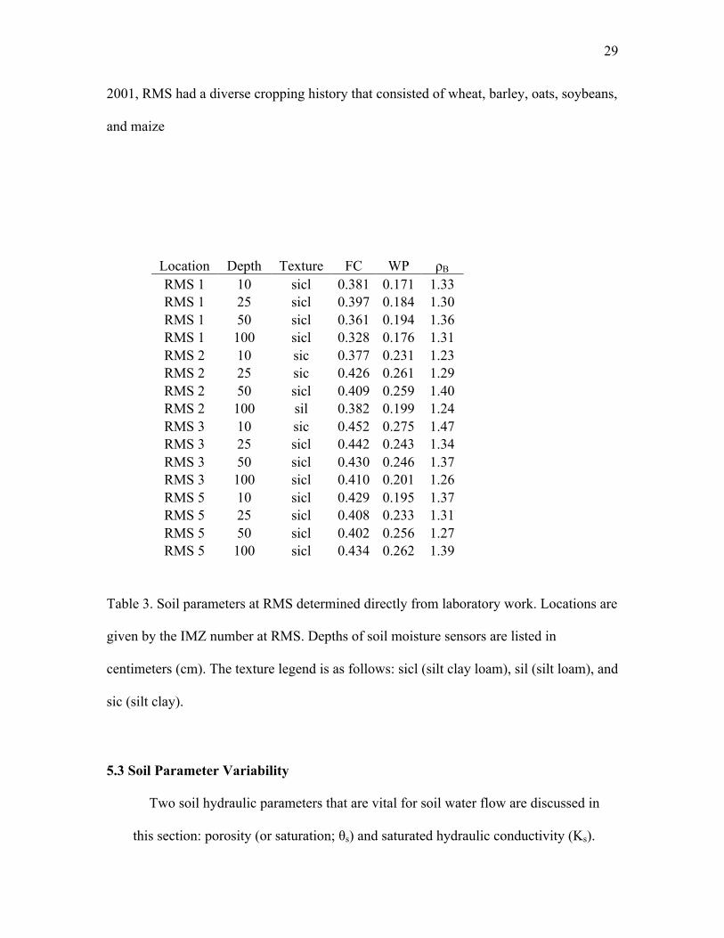
5.2.3 RMS
Soils at RMS are a mix of the Fillmore, Tomek, Yutan, and Filbert series and are
mostly silt clay loam in texture. Soils at RMS are deep and high in organic matter. Bulk
densities at RMS average 1.35 Mg/m3, 1.31 Mg/m3, 1.35 Mg/m3, and 1.30 Mg/m3 at 10
cm, 25 cm, 50 cm, and 100 cm respectively (Table 3). Prior to the beginning of CSP in
29
2001, RMS had a diverse cropping history that consisted of wheat, barley, oats, soybeans,
and maize
Location Depth Texture FC WP ρB RMS 1 10 sicl 0.381 0.171 1.33 RMS 1 25 sicl 0.397 0.184 1.30 RMS 1 50 sicl 0.361 0.194 1.36 RMS 1 100 sicl 0.328 0.176 1.31 RMS 2 10 sic 0.377 0.231 1.23 RMS 2 25 sic 0.426 0.261 1.29 RMS 2 50 sicl 0.409 0.259 1.40 RMS 2 100 sil 0.382 0.199 1.24 RMS 3 10 sic 0.452 0.275 1.47 RMS 3 25 sicl 0.442 0.243 1.34 RMS 3 50 sicl 0.430 0.246 1.37 RMS 3 100 sicl 0.410 0.201 1.26 RMS 5 10 sicl 0.429 0.195 1.37 RMS 5 25 sicl 0.408 0.233 1.31 RMS 5 50 sicl 0.402 0.256 1.27 RMS 5 100 sicl 0.434 0.262 1.39
Table 3. Soil parameters at RMS determined directly from laboratory work. Locations are
given by the IMZ number at RMS. Depths of soil moisture sensors are listed in
centimeters (cm). The texture legend is as follows: sicl (silt clay loam), sil (silt loam), and
sic (silt clay).
5.3 Soil Parameter Variability
Two soil hydraulic parameters that are vital for soil water flow are discussed in
this section: porosity (or saturation; θs) and saturated hydraulic conductivity (Ks).
30
The former was obtained from field samples and the latter was calculated via
pedotransfer functions (PTF’s) given in Saxton and Rawls (2006). Soil hydraulic
parameters can also be estimated via remotely sensed soil moisture (Santanello et
al. 2007; Harrison et al. 2012) and are critical for determining soil moisture in land
surface models such as the Noah land surface model (Ek et al. 2003).
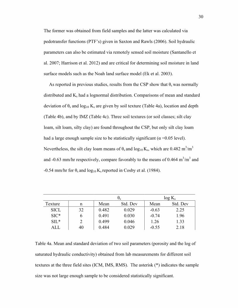
As reported in previous studies, results from the CSP show that θs was normally
distributed and Ks had a lognormal distribution. Comparisons of mean and standard
deviation of θs and log10 Ks are given by soil texture (Table 4a), location and depth
(Table 4b), and by IMZ (Table 4c). Three soil textures (or soil classes; silt clay
loam, silt loam, silty clay) are found throughout the CSP, but only silt clay loam
had a large enough sample size to be statistically significant (α =0.05 level).
Nevertheless, the silt clay loam means of θs and log10 Ks, which are 0.482 m3/m3
and -0.63 mm/hr respectively, compare favorably to the means of 0.464 m3/m3 and
-0.54 mm/hr for θs and log10 Ks reported in Cosby et al. (1984).
θs log Ks Texture n Mean Std. Dev Mean Std. Dev
SICL 32 0.482 0.029 -0.63 2.25 SIC* 6 0.491 0.030 -0.74 1.96 SIL* 2 0.499 0.046 1.26 1.33
ALL 40 0.484 0.029 -0.55 2.18 Table 4a. Mean and standard deviation of two soil parameters (porosity and the log of
saturated hydraulic conductivity) obtained from lab measurements for different soil
textures at the three field sites (ICM, IMS, RMS). The asterisk (*) indicates the sample
size was not large enough sample to be considered statistically significant.
31
θs log (Ks) Location and Depth n Textures Mean Std. Dev. Mean Std. Dev. ICM 10 cm 1 0.525 0.021 2.25 0.83 ICM 25 cm 1 0.494 0.016 0.20 0.84 ICM 50 cm 3 0.463 0.017 -1.60 2.64 ICM 100 cm 2 0.463 0.006 -2.11 1.03 IMS 10 cm 1 0.444 0.007 -2.06 2.23 IMS 25 cm 1 0.485 0.029 -0.55 2.18 IMS 50 cm 1 0.471 0.024 -2.13 2.21 IMS 100 cm 1 0.479 0.017 -2.08 2.33 RMS 10 cm 2 0.503 0.023 0.43 1.85 RMS 25 cm 2 0.506 0.008 0.51 1.04 RMS 50 cm 1 0.491 0.021 0.43 1.32 RMS 100 cm 2 0.510 0.025 1.19 1.93
Table 4b. Mean and standard deviation of two soil parameters (porosity and the log
of saturated hydraulic conductivity) obtained from lab measurements for 12
location and depth combinations at ICM, IMS, and RMS respectively.
32
θs log (Ks) IMZ n(Textures) Mean Std. Dev. Mean Std. Dev.
ICM 4 3 0.491 0.031 -0.06 2.31 ICM 5 2 0.495 0.037 0.40 2.11 ICM 6 1 0.473 0.023 -1.29 2.48
IMS 2 1 0.453 0.025 -1.80 1.86 IMS 5 1 0.464 0.023 -3.41 1.45 IMS 6 1 0.461 0.022 -1.94 2.10
RMS 1 1 0.500 0.009 1.87 0.53 RMS 2 3 0.513 0.030 1.16 1.31 RMS 3 2 0.499 0.018 -0.53 1.38 RMS 5 1 0.496 0.025 0.05 1.38
Table 4c. Mean and standard deviation of two soil parameters (porosity and the log
of saturated hydraulic conductivity) over all depths for IMZ’s with soil water at
ICM, IMS, and RMS. The number of soil textures in a soil profile at a given
location is given in the second column from the left.
Previous studies (Gutmann and Small, 2005; Cosby et al. 1984) reported
large variation in hydraulic parameters existed in other soil databases; thus it was
not unexpected that variation (i.e., the standard deviation) in Ks at Mead was
sometimes greater within a field or within an IMZ than across the entire study area.
For example, the variation in Ks across the 50 cm depth of IMZ’s at ICM and
across all depths of IMZ’s at IMS was larger than the variation across the entire
study area (Table 3b). Two individual IMZ’s (ICM 4, ICM 6) also had more
variation in Ks within the soil profile than across the whole field (Table 3c).
Variation in θs was less within fields and within IMZ’s than across the entire study
except across the 25 cm depth of IMZ’s at IMS where the variation equaled that of
the entire study area. Variation was generally less at RMS for both Ks and θs than at
33
the two irrigated sites. For example, the highest standard deviation in the profile at
any RMS IMZ was 1.38, which is lower than the standard deviation at any IMZ at
ICM and IMS (Table 3c). This would imply more uniformity in the geometrical
pore structure within the soil (Klute and Dirksen, 1986) at RMS but data are not
available to prove that.
The amount of vertical and spatial variation in Ks differed between fields as
well. Variation in Ks was significantly higher within the soil profile of an IMZ at
ICM than at the same depth (i.e., 50 cm) across the field. Conversely, IMS had
significantly higher spatial variation than vertical variation in Ks. Spatial variation
in Ks was slightly higher than vertical variation in Ks at RMS. Soil texture was
generally homogeneous throughout the CSP, with six of ten IMZ’s having only one
soil texture class (silt clay loam) and of all 40 samples, 32 of them were a silt clay
loam.
6.0 Dissertation Organization
Each of these research questions highlighted earlier will be addressed in
its own research chapter. Since soil water is the overarching theme throughout the
dissertation, there is some overlap in data presented in each chapter. The three
research chapters (Chapters 2 through 4) presented here have been written up in the
format of a publishable paper and Chapter 4 was published in Agricultural and
Forest Meteorology in 2014. Thus, each chapter also has information pertaining to
the study site, which means there is also overlap in a few tables presented here.
However, all table and figure numbers restart with the beginning of a new chapter.
34
Chapter 2: A soil water climatology of a rainfed field in eastern Nebraska
The objective of this chapter is to determine the relationship between soil
moisture and precipitation at a rainfed agroecosystem over a period of eight years
that included historically wet, historically dry, and average conditions compared to
a 30-year period of record for the location. Soil moisture data from the rainfed
agroecosystem (RMS) are compared to those of the irrigated agroecosystem (IMS)
to better demonstrate the loss of soil moisture during dry spells at RMS.
Measurements from RMS are also compared to a30-year precipitation climatology
at Mead and a precipitation climatology at two High Plains sites and three other
sites in the Corn Belt.
Chapter 3: The dynamic relationship between soil moisture and biophysical measurements over a maize field
The objective of this chapter is to determine the relationship of field-
scale averaged soil moisture and biophysical variables, such as evapotranspiration
and gross primary productivity, and its effect on the surface energy budget at both
a rainfed and irrigated maize field. This chapter also shows how the lack of soil
water at RMS affected the partitioning of the energy balance compared to the well-
watered IMS and how significant precipitation events during dry spells led to
increases, albeit brief, in implied stomatal conductance of maize plants at RMS.
35
Chapter 4: Monitoring the effects of rapid onset of drought on non-
irrigated maize with agronomic data and climate-based drought indices
The objective of this chapter is to present a detailed analysis of a flash
drought that occurred at Mead in 2003. The flash drought began in late June and
lasted through the most critical time of the growing season for maize- the late
vegetative and the reproductive stage. In this chapter, two standardized drought
indices, the Standardized Precipitation Index (SPI) and the Standardized
Precipitation Evapotranspiration Index (SPEI) are compared to soil water and
biophysical data from IMS to demonstrate their utility at depicting a rapidly
developing drought. Data from RMS are also compared to neighboring IMS to
demonstrate the effectiveness and usefulness of irrigation during such a period.
36
7.0 References: Alley, W. M. 1984: The Palmer drought severity index: Limitations and
applications. J. Appl. Meteor., 23, 1100–1109.
Anderson, M. C., J. M. Norman, G. R. Diak, W. P. Kustas, and J. R. Mecikalski,
1997: A two-source time-integrated model for estimating surface fluxes using
thermal infrared remote sensing. Remote Sens. Environ., 60, 195–216.
Anderson, M.C., J. M. Norman, J. R. Mecikalski, J. A. Otkin, and W. P. Kustas,
2007b: A climatological study of evapotranspiration and moisture stress across the
continental U.S. based on thermal remote sensing: 1. Model formulation. J.
Geophys. Res., 112, D10117.
Anderson, M.C., C. Hain., J. A. Otkin, X. Zhan, K. Mo, M. Svoboda, B. Wardlow,
And A. Pimstein, 2013: An intercomparison of drought indicators based on thermal
remote sensing and NLDAS simulations. J. Hydrometeor.,14, 1035–1056,
Arndt, D. S., H.L. Johnson. 2002. The value of real-time mesoscale observations to
early recognition and rapid response to short-term drought.
Basara, J.B., D.S. Arndt, H.L. Johnson, et al. 1998: An analysis of the drought of
1998 using the Oklahoma Mesonet. EOS Trans., AGU, 79, 258.
37
Best, M.J., Pryor, M., Clark, D.B., Rooney, G.G., Essery, R.L.H., Menard, C.B.,
Edwards, J.M., Hendry, M.A., Porson., A., Gedney, N., Mercado, L.M., Sitch, S.,
Blyth, E., Boucher, O., Cox, P.M., Grimmond, C.S.B., Harding, R.J., 2011. The
Joint UK Land Environment Simulator (JULES), model and description- Part 1:
Energy and water fluxes. Geosci. Model Dev., 4, 677-699.
Bleed, A., P.E. Emeritus, C.H. Babbitt, 2015. Nebraska’s Natural Resources
Districts: An assessment of a large-scale locally controlled water governance
framework. Policy Report 1 of the Robert B. Daugherty Water for Food Institute.
Calvino, P.A., Andrade, F.H., Sadras, V.O., 2003. Maize yield as affected by water
availability, soil depth, and crop management. Agron. J. 95, 275-281.
Chapman, S.S., Omernik, J.M., Freeouf, J.A., Huggins, D.G., McCauley, J.R.,
Freeman, C.C., Steinauer, G., Angelo, G.T., and Schlepp, R.L. 2001. Ecoregions of
Nebraska and Kansas. U.S. Geological Survey, Reston, VA. Scale 1:1,950,000.
Cosby, B.J., Hornberger, G.M., Clapp, R.B., Ginn, T.R., 1984. A statistical
exploration of the relationships of soil moisture characteristics to the physical
properties of soils. Water Resour. Res. 20, 682-690.
Ek, M.B., Mitchell, K.E., Lin Y., Rogers, E., Grunmann, P., Koren,V., Gayno, G.,
Tarpley, J.D. 2003. Implementation of Noah land surface model advances in the
38
National Centers for Environmental Prediction operational mesoscale Eta model, J.
Geophys. Res. 108(D22), 8851, doi:10.1029/2002JD003296.
Guttman, N. B. 1998. Comparing the Palmer Drought Index and the Standardized
Precipitation Index. J. Amer. Water Resour. Assoc., 34, 113–121.
Guttman, N.B. 1999. Accepting the Standardized Precipitation Index: A calculation
algorithm. J. Amer. Water Resour. Assoc., 35, 311-322.
Gutmann, E.D., Small, E.E. 2005. The effect of soil hydraulic properties vs. soil
texture in land surface models. Geophys. Res. Lett., 32, doi:
10.1029/2004GL021843.
Harrison, K.W., Kumar, S.V., Peters-Lidard, C.D., Santanello, J.A., 2012.
Quantifying the change in soil moisture modeling uncertainty from remote sensing
observations using Bayesian inference. Water Resour. Res., 48, W11514,
doi:10.1029/2012WR012337.
Hayes, M., D. A. Wilhite, M. Svoboda, and O. Vanyarkho. 1999. Monitoring the
1996 drought using the standardized precipitation index. Bull. Amer. Meteor. Soc.,
80, 429–438.
39
Hillel, D., 2004. Introduction to Environmental Soil Physics. Elsevier Academic
Press, San Diego.
Heim, R. R., 2002: A review of twentieth-century drought indices used in the
United States. Bull. Amer. Meteor. Soc., 83, 1149–1165.
Hu, Q., G. D. Willson. 2000. Effect of temperature anomalies on the Palmer
drought severity index in the central United States. Int. J. Climatol., 20, 1899–
1911.
Klute, A., Dirksen, C., 2007. Hydraulic conductivity and diffusivity, laboratory
methods. p. 687-732. In Klute (ed.) Methods of soil analysis. SSSA, Madison, WI.
Livida, I., Assemakopoulos, V.D. 2007. Spatial and temporal analysis of drought in
Greece using the Standardized Precipitation Index (SPI). Theoret. Appl. Climatol.
89, 143-153.
Lloyd-Hughes, B., M. A. Saunders. 2002. A drought climatology for Europe. Int. J.
Climatol., 22, 1571–1592.
McKee, T. B., Doesken, N.J., Kleist, J., 1993. The relationship of drought
frequency and duration to time scales. Preprints, Eighth Conf. on Applied
Climatology. Anaheim, CA, Amer. Meteor. Soc., 179–184.
40
McRoberts, B., Nielsen-Gammon, J. 2012. The Use of a High-Resolution
Standardized Precipitation Index for Drought Monitoring and Assessment. J. Appl.
Met. Climatol. 51 (1), 68-83.
Mavromatis, T., 2007. Drought index evaluation for assessing future wheat
production in Greece. Int. J. Climatol., 27 (7), 911-924.
Monteith, J.L., 1964. Evaporation and environment. The State and Movement of
Water in Living Organisms, 19th Symp. Soc. Biol., Academic Press, NY, pp. 205-
234.
Otkin, J.A., Anderson, M.C., Hain, C., Svoboda, M., 2014. Examining flash
drought development and the rapid changes in the evaporative stress index. J.
Hydrometeor., 14, 1057-1074.
Otkin, J.A., Anderson, M.C., Hain, C., Svoboda, M., 2015. Using temporal
changes in drought indices to generate probalisitic drought intensification
forecasts. J. Hydrometeor., 16, 88-105.
Palmer, W. C. 1965. Meteorological droughts. U.S. Department of Commerce,
Weather Bureau Research Paper 45, 58 pp.
41
Peterson, T.C., Easterling, WD.R., Karl, T.A., Groisman, P., Nicholls, N.,
Plummer, N., Torok, S., Auer, I., Boehm, R., Gullett, D., Vincent, L., Heino, R.,
Tuomenvirta, H., Mestre, O., Szentimrey, T., Salinger, J., Forland, Hanssen-Bauer,
I., Alexandersson, H., Jones, P., Parker, D. 1998. Homogeneity adjustments of in
situ atmospheric climate data: A review. Int. J. Climatol., 18: 1493-1517.
Santanello, J. A., Peters-Lidard, C., Garcia, M., Mocko, D., Tischler, M., Moran,
M. S., Thoma, D.P. , 2007. Using Remotely-Sensed Estimates of Soil Moisture to
Infer Spatially Distributed Soil Hydraulic Properties. Remote Sensing Environ.
110, 79-97.
Saxton, K.E., Rawls, W.J., 2006. Soil water characteristic estimates by texture and
organic matter for hydrologic solutions. Soil Sci. Am. J. 70, 1569-1578
Suyker, A.E., Verma, S.B., Burba, C.G. 2003. Interannual variability in net CO2
exchange of a native tallgrass prairie. Global Change Biol. 9, 1-11.
Suyker, A.E., Verma, S.B., Burba, G.G., Arkebauer, T.J., Walters, D.T., Hubbard,
K.G., 2004. Growing season carbon dioxide exchange in irrigated and rainfed
maize, Agric. For. Meteorol. 124, 1-13.
Suyker, A. E., Verma, S.B., 2008. Interannual water vapor and energy exchange in
an irrigated maize-based agroecosystem. Agricul. For. Meteorol. 148, 417-427.
42
Suyker, A. E., Verma, S.B., 2009. Evapotranspiration of irrigated and rainfed
maize-soybean cropping systems. Agricul. For. Meteorol. 149, 443-452.
Suyker, A.E., Verma, S.B., 2012. Gross primary production and ecosystem
respiration of irrigated and rainfed maize-soybean cropping system over 8 years.
Agric. For. Meteorol. 165, 12-24.
Thornthwaite, C.W. 1948. An approach toward a rational classification of climate.
Geogr. Rev., 38, 55-94.
Verma, S.B., Dobermann, A., Cassman, K.G., Walters, D.T., Knops, J.M.,
Arkebauer, T.J., Suyker, A.E., Burba, G.G., Amos, B., Yang, H., Ginting, D.,
Hubbard, K.G., Gitelson, A.A., Walter-Shea, E.A., 2005. Annual carbon dioxide
exchange in irrigated and rainfed maize-based agroecosystems. Agricul. For.
Meteorol. 131, 77-96.
Vinnikov, K.Y., Robock, A., Qiu, S., Entin, J.K., Owe, M., Choudhury, B.J.,
Hollinger, S.E., Njoku, E.G., 1999. Satellite remote sensing of soil moisture in
Illinois, United States. J. Geophys. Res. 104, 4145-4168.

43
Wu, H., Hayes, M.J., Wilhite, D.A., Svoboda, M.D., 2005. The effect of length of
record on the standardized precipitation index calculation. Int. J. Climatol. 25 (4),
505-520.
44
CHAPTER 2: A SOIL MOISTURE CLIMATOLOGY OF A RAINFED FIELD IN EASTERN NEBRASKA Abstract:
The objective of this chapter is to show results from eight years of soil
moisture measurements under a rainfed agroecosystem in a region that is uniquely
situated in a transition zone between almost exclusively rainfed agriculture to the
east and almost exclusively irrigated agriculture to the west. Soil moisture sensors
were installed at four depths (10 cm, 25 cm, 50 cm, and 100 cm) in Intensive
Management Zones (IMZ's) for the purpose of determining crucial plant-soil
moisture relationships under maize and soybeans, both irrigated and rainfed
conditions,, as part of the Carbon Sequestration Project (CSP) at Mead, NE. The
eight years (2002-2009) of soil moisture data utilized in this study captured a range
of different growing season conditions ranging from drought and flash drought
events to periods significantly above-average precipitation. Soil moisture at the
rainfed site correlated well with precipitation over the entirety of the study period.
However, this paper shows that timing of precipitation was often more important to
differences in average seasonal soil moisture than total growing season (May-
October) precipitation, as total growing season precipitation did not always reflect
within-season variability of precipitation. This paper shows that shallow soil
moisture was most reflective of an incipient wet or dry spell within a season and
deeper soil moisture was most reflective of longer-term dryness or wetness. Data
from a nearby irrigated field were also analyzed to further demonstrate the
importance of variability and timing of precipitation within a season, as it was
critical to scheduling irrigation treatments at the irrigated site.
45
1.0. Introduction
This chapter resents results obtained from the analysis of eight years of soil
moisture measurements at various depths under a rainfed agroecosystem an area
located in the transition zone between rainfed-dominated agriculture in the U.S.
Corn Belt and more intensively irrigated agriculture in the U.S. Great Plains
region. Soil moisture is an integral part of the hydrologic cycle and a critical
parameter for plant growth and development. Soil moisture measurements, both in-
situ and satellite-derived estimates (Nghiem et al. 2012), are utilized for drought
monitoring and predictions of flash flooding at a local or regional scale and for
land surface modeling on regional to global scales. With the introduction of an
optimization and data assimilation framework such as the NASA Land Information
System (LIS; Kumar et al. 2006; Peters-Lidard et al. 2007), in-situ soil moisture
measurements can be utilized for data assimilation (Kumar et al. 2008; Kumar et
al. 2012) and estimation of soil hydraulic parameters, such as porosity and
saturated hydraulic conductivity (Santanello et al. 2007; Harrison et al. 2012).
Thus, there is likely to be increasing demand from the land surface modeling
community to utilize real-time soil moisture measurements, including those under
crop cover.
Unfortunately, in-situ soil moisture measurements under crop cover have
been somewhat limited compared to measures under other land cover types (e.g.,
grass) to date, but important insights into the soil moisture-crop response have been
made. Nielsen et al. (2010) showed that rainfed maize yields in northeast Colorado
46
were highly correlated to precipitation between 16 July and 26 August and the
chances for a “break-even” yield were substantially higher if sufficient soil
moisture was available at planting. Meyer et al. (1993a) reported that maize was
most sensitive to water stress in the silking-blister dough stage. Calvino et al.
(2003) reported a curvilinear response of maize yield to available water in the three
weeks preceding and following silking. Earl and Davis (2003) reported maize yield
reductions up to 85% during severe water stress that occurred after the sixth leaf
stage in Georgia. Soybean (Glycine max L.) yields are reduced significantly when
water stress occurs during flowering and pod fill stages. Doss et al. (1974) and Eck
et al. (1987) reported soybean yield reductions of 50 percent when water stress
occurred between the flowering and beginning seed stage. Thus, it is well
established that a lack of soil moisture causes vegetation stress and yield reduction
during the critical growth stage(s) of crops.
Illston et al. (2004) found four distinct soil moisture phases during the year
under grass cover at Oklahoma Mesonet sites that included: 1) a moist plateau in
the spring, 2) a transitional drying in early summer, 3) an enhanced drying later in
the summer, and 4) a recharge phase in the autumn and winter. Similar seasonal
trends were also noted at Automated Weather Data Network (AWDN) sites in
Nebraska (Hubbard et al. 2009a). In that case, Hunt et al. (2009) showed there was
a longitudinal gradient of decreasing east-to-west precipitation that led to
corresponding decreasing east-to-west gradients in soil moisture in the summer and
early autumn.
47
Soil moisture gradients in the Illinois Soil Moisture Network varied by
latitude in the winter and spring versus longitude in the summer and autumn, and
an average depletion of 72 mm in the top 2 m of soil was found at sites throughout
the state between the winter and summer months (Hollinger and Isard, 1994).
Vinnikov et al. (1999) add that a standard deviation of 8.5% in volumetric water
content existed in the top 10 cm of soil across the Illinois Soil Moisture Network
over a six-year period in the 1980’s. Scott et al. (2010) also found that volumetric
water content variability increased with depth between sites in a sod experiment in
east-central Illinois and noted a strong relationship between observed soil moisture
in the deeper layers and surface terrain slope.
Irrigated agriculture, like rainfed agriculture, continues to serve an
important role in the production of cereal crops, with increasing importance in the
developing world. Many areas however, including the U.S. High Plains region, are
faced with the daunting task of increasing crop production with less water, as
groundwater reserves become further depleted (Sophocleous, 2012). Climate
change could further exacerbate limited supplies of groundwater in these regions.
Thus, monitoring soil moisture under cereal crops is critical for determining the
best irrigation strategies and other farming practices, such as no-till or reduced till.
In an ideal situation, soil moisture measurements under crop cover would
be common on a global scale and utilized for data assimilation. Unfortunately,
long-term studies of soil moisture under crop cover on a field scale, such as the 25-
year study reported by Nielsen et al. (2010), have been rare. Thus, a crucial need
for long-term soil moisture measurements under irrigated and rainfed crops, such

48
as maize, was met when soil moisture sensors were installed as part of a large
carbon and energy balance project called the Carbon Sequestration Project (CSP;
Suyker et al. 2004; Verma et al. 2005) at the UNL research farm near Mead, NE.
The long period of time over which soil moisture data were collected in the CSP,
the diversity of crops and management practices under which the data were
collected, and the range in meteorological conditions between growing seasons
allow this study to have applicability beyond Nebraska and the U.S. Corn Belt for
the key cash crops of maize and soybeans. Therefore, the overall goal of this paper
is to show the variability of soil moisture under crop cover over an eight-year
period at a location in a transition zone between (almost) exclusively rainfed
agriculture to the east and irrigated agriculture to the west.
The location in the transition zone allows for the possibility that soil
moisture measurements under crop cover in a wet year could potentially be
representative of a typical season at locations further east in the U.S. Corn Belt.
Conversely, it is possible that the soil moisture measurements from Mead could be
representative of a rainfed field in the High Plains in a dry season. Given the
importance of irrigation for high-yielding crops in a semi-arid area like the High
Plains, the comparison of soil moisture under a rainfed field to soil moisture under
an irrigated field in a flash drought shows the value of having irrigation to offset
the lack of natural precipitation. Likewise, soil moisture measurements under a
rainfed field can be very useful in better determining the relationship between soil
moisture and crop stress at the field scale during a flash drought.
49
2.0 Materials and methods
2.1 Carbon Sequestration Project site
The CSP is located at the University of Nebraska-Lincoln (UNL)
Agricultural Research and Development Center in Saunders County, Nebraska near
the town of Mead. This location is roughly 35 km northeast of Lincoln, NE and is
defined in Chapman et al. (2001) as being at the western edge of the Western Corn
Belt Plains ecoregion. Maize and soybeans are the main crops grown in the area
and according to the National Agricultural Statistics Service (NASS), about 67
percent of crops grown in Saunders County, NE where the study area is located
were rainfed in the final year of the study period (2009).
This region is a sharp transition zone between almost exclusively rainfed
agriculture in far eastern Nebraska that extends into the adjacent Corn Belt region
to the east and the predominatelyirrigated agriculture to the west that extends into
the semi-arid Great Plains. For example, Cass County, NE (just east-southeast
along the Missouri River) was 99 percent rainfed in the final year of the study
period. Meanwhile, in the same year in Merrick County, NE, which is 100 km west
of the CSP sites, 94 percent of the crops were irrigated. Thus, the rainfed and
irrigated fields of the CSP make it representative of the aforementioned transition
zone in eastern Nebraska.
The CSP was initiated in the spring of 2001 and consisted of three field
sites ranging in size from 49 to 65 ha. The first site has been managed as an
irrigated, continuous maize (ICM) site centered at 41˚09’54.2” N, 96˚ 28’35.9” W.
The second site has supported an irrigated, maize-soybean (IMS) rotation (inter-
50
annual) located at 41˚09’53.5” N, 96˚ 28’12.3” W. The third site is a rainfed,
rotated maize-soybean (RMS) system located at 41˚10’46.8” N, 96˚ 26’22.7” W.
Most of the data used for this study was collected at RMS as its data best reflect the
variability of precipitation within the study period because it was a rainfed system.
Data from IMS are used for comparisons, as the crop type was the same as RMS in
every growing season during this study. Data from ICM, while unique, are
excluded from analysis in this chapter half the years because odifferent crops were
planted (i.e., maize and soybeans). Second, management practices varied (i.e.,
continuous maize and a switch from no-till to conservation tillage halfway through
the study period) that could inter-field soil moisture differences not related to
natural precipitation or irrigation applications, which was not the focus of this
research.
Maize was planted to IMS and RMS in odd numbered years and soybeans
in even numbered years. The dates of specific development stages of maize and
soybeans at the three sites were determined from records collected during regular
field analyses by agronomists. There was usually a slight variation in a
development stage within the three fields, so the date listed for a particular
development stage of maize was when the majority of the crop in the field was at
that stage. Reproductive stage was considered to have begun when field samples
showed greater than 50 percent of a field with a maize (soybean) crop entering
silking (beginning bloom). Soybeans and maize both reached physiological
maturity in September, with maize typically reaching that stage slightly earlier in
the month. Harvest dates were heavily influenced by weather and ranged from
51
early October to early November. Later harvest dates were usually a result of wet
conditions in October, especially in 2009 when unusually wet and cool conditions
persisted throughout the month.
Maize planting density at RMS was about 75 percent of the density at IMS,
with an average of approximately 62,000 plants/ha over the four years compared to
an average planting density of 81,936 plants/ha for IMS. The planting density for
soybeans was 370,644 plants/ha for each year soybeans were planted at IMS and
RMS. Planting density for maize at RMS was lower than at IMS to limit plant
competition for soil moisture in a rainfed field during dry periods. Yields for maize
averaged 13.7 and 9.8 Mg/ha at IMS and RMS, respectively. Yields for soybeans
averaged 3.7 and 3.4 Mg/ha at IMS and RMS, respectively. For additional details,
please refer to Verma et al. (2005) and Suyker et al. (2003).
2.2 Intensive Management Zones and soil parameters
Each CSP site contained six 20 m-by-20 m IMZ’s, where detailed process-
level measurements of soil moisture, soil C dynamics, canopy and soil gas
exchange, crop growth and biomass partitioning were collected. Root distribution
measurements, however, were not made during the study period and thus, root
densities at specific depths are unknown. The two field sites were uniformly tilled
by disking the top 10 cm at the beginning of the study to incorporate Phosphorous
(P) and Potassium (K) fertilizers and to homogenize the soil layer (Suyker and
Verma, 2009). Table 1 shows details about crop management, cultivars, final grain
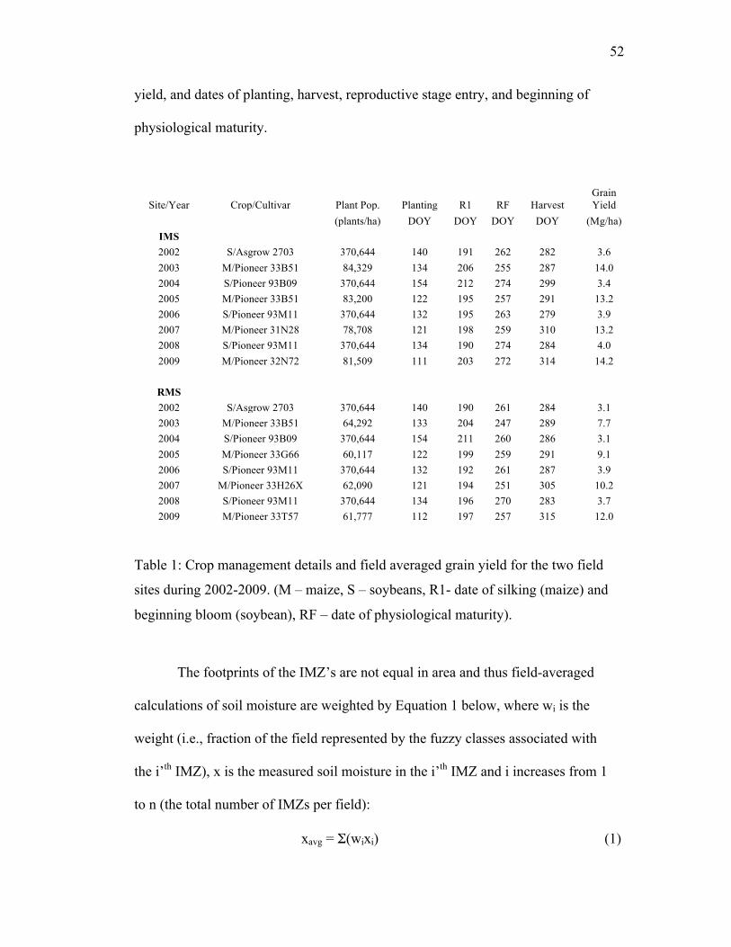
52
yield, and dates of planting, harvest, reproductive stage entry, and beginning of
physiological maturity.
Site/Year Crop/Cultivar Plant Pop. Planting R1 RF Harvest Grain Yield
(plants/ha) DOY DOY DOY DOY (Mg/ha) IMS 2002 S/Asgrow 2703 370,644 140 191 262 282 3.6 2003 M/Pioneer 33B51 84,329 134 206 255 287 14.0 2004 S/Pioneer 93B09 370,644 154 212 274 299 3.4 2005 M/Pioneer 33B51 83,200 122 195 257 291 13.2 2006 S/Pioneer 93M11 370,644 132 195 263 279 3.9 2007 M/Pioneer 31N28 78,708 121 198 259 310 13.2 2008 S/Pioneer 93M11 370,644 134 190 274 284 4.0 2009 M/Pioneer 32N72 81,509 111 203 272 314 14.2
RMS 2002 S/Asgrow 2703 370,644 140 190 261 284 3.1 2003 M/Pioneer 33B51 64,292 133 204 247 289 7.7 2004 S/Pioneer 93B09 370,644 154 211 260 286 3.1 2005 M/Pioneer 33G66 60,117 122 199 259 291 9.1 2006 S/Pioneer 93M11 370,644 132 192 261 287 3.9 2007 M/Pioneer 33H26X 62,090 121 194 251 305 10.2 2008 S/Pioneer 93M11 370,644 134 196 270 283 3.7 2009 M/Pioneer 33T57 61,777 112 197 257 315 12.0
Table 1: Crop management details and field averaged grain yield for the two field
sites during 2002-2009. (M – maize, S – soybeans, R1- date of silking (maize) and
beginning bloom (soybean), RF – date of physiological maturity).
The footprints of the IMZ’s are not equal in area and thus field-averaged
calculations of soil moisture are weighted by Equation 1 below, where wi is the
weight (i.e., fraction of the field represented by the fuzzy classes associated with
the i’th IMZ), x is the measured soil moisture in the i’th IMZ and i increases from 1
to n (the total number of IMZs per field):
xavg = Σ(wixi) (1)
53
Weights were assigned to each IMZ based on the proportional area of the fuzzy
class represented. Not all IMZ’s had soil moisture at all four depths, with some
IMZ’s only having it at 10 cm. Thus, soil moisture is only reported at IMZ’s with
soil moisture at all depths for the sake of consistency.
Prior to this study, soil samples were collected from IMZ’s of the two sites
and then analyzed in the laboratory for water retention curves and soil parameters,
such as bulk density. Saturation (θs) values were calculated from bulk density
values obtained from the laboratory. Field capacity (θFC) and wilting point (θWP)
values were determined from moisture release curves obtained from laboratory
work and saturated hydraulic conductivity (Ks) was calculated from
aforementioned values of θFC, θWP, and θs using algorithms in Saxton and Rawls
(2006).
Results from the IMZs show that θs was normally distributed and Ks had a
lognormal distribution. Comparisons of mean and standard deviation of θs and
log10 Ks are given by location and depth (Table 2a) and by IMZ (Table 2b) at IMS
and RMS. Soil texture is generally homogeneous throughout the CSP, with several
IMZ’s having only one soil texture class (silt clay loam) and of all 40 samples
(including those from ICM), 32 of them were considered a silt clay loam texture.
Other soil textures (or soil classes; silt loam and silty clay) are found throughout
the CSP, but only silt clay loam had a large enough sample size to be statistically
significant (α =0.05 level). Nevertheless, the silt clay loam means of θs and log10
Ks, which are 0.482 m3/m3 and -0.63 mm/hr, respectively, compare favorably to the
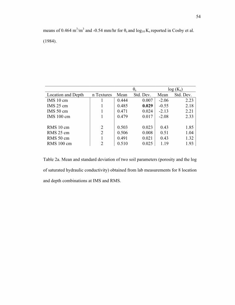
54
means of 0.464 m3/m3 and -0.54 mm/hr for θs and log10 Ks reported in Cosby et al.
(1984).
θs log (Ks) Location and Depth n Textures Mean Std. Dev. Mean Std. Dev. IMS 10 cm 1 0.444 0.007 -2.06 2.23 IMS 25 cm 1 0.485 0.029 -0.55 2.18 IMS 50 cm 1 0.471 0.024 -2.13 2.21 IMS 100 cm 1 0.479 0.017 -2.08 2.33 RMS 10 cm 2 0.503 0.023 0.43 1.85 RMS 25 cm 2 0.506 0.008 0.51 1.04 RMS 50 cm 1 0.491 0.021 0.43 1.32 RMS 100 cm 2 0.510 0.025 1.19 1.93
Table 2a. Mean and standard deviation of two soil parameters (porosity and the log
of saturated hydraulic conductivity) obtained from lab measurements for 8 location
and depth combinations at IMS and RMS.
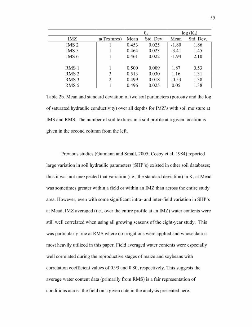
55
θs log (Ks) IMZ n(Textures) Mean Std. Dev. Mean Std. Dev.
IMS 2 1 0.453 0.025 -1.80 1.86 IMS 5 1 0.464 0.023 -3.41 1.45 IMS 6 1 0.461 0.022 -1.94 2.10
RMS 1 1 0.500 0.009 1.87 0.53 RMS 2 3 0.513 0.030 1.16 1.31 RMS 3 2 0.499 0.018 -0.53 1.38 RMS 5 1 0.496 0.025 0.05 1.38
Table 2b. Mean and standard deviation of two soil parameters (porosity and the log
of saturated hydraulic conductivity) over all depths for IMZ’s with soil moisture at
IMS and RMS. The number of soil textures in a soil profile at a given location is
given in the second column from the left.
Previous studies (Gutmann and Small, 2005; Cosby et al. 1984) reported
large variation in soil hydraulic parameters (SHP’s) existed in other soil databases;
thus it was not unexpected that variation (i.e., the standard deviation) in Ks at Mead
was sometimes greater within a field or within an IMZ than across the entire study
area. However, even with some significant intra- and inter-field variation in SHP’s
at Mead, IMZ averaged (i.e., over the entire profile at an IMZ) water contents were
still well correlated when using all growing seasons of the eight-year study. This
was particularly true at RMS where no irrigations were applied and whose data is
most heavily utilized in this paper. Field averaged water contents were especially
well correlated during the reproductive stages of maize and soybeans with
correlation coefficient values of 0.93 and 0.80, respectively. This suggests the
average water content data (primarily from RMS) is a fair representation of
conditions across the field on a given date in the analysis presented here.
56
2.3 Soil moisture sensors
Dynamax Theta probes were installed in the spring of 2001 at depths of 10,
25, 50, and 100 cm as part of three IMZ’s in ICM and IMS, and four in RMS. The
soil moisture probes were installed at a 45° angle orthogonal to the surface at 10
and 25 cm and were installed using the drip loop method at 50 and 100 cm. Soil
moisture sensors were always removed at 10 cm and 25 cm for planting and
harvest at all sites. Impedance probes contain a waterproof enclosure, sensing head,
and a cable. The enclosure has a measurement circuitry and an oscillator, while the
sensor head consists of three outer rods that shield an inner rod. The rods act as a
transmission line and have an impedance that is dependent on the dielectric
constant of the soil. Topp et al. (1980) showed that a linear relationship exists
between the volumetric water content and the dielectric constant. Thus, soil
volumetric water content (θ) is the standard soil moisture variable in the CSP, and
the broader network of sensors across the state as part of the Nebraska Automated
Weather Data Network (AWDN; Hubbard et al. 2009; You et al. 2010).
Soil moisture data from the CSP underwent significant quality control
before its release. Data were replaced by previous day's values if one day was bad
(e.g., sensor issue) and by linear interpolation if more than one day was bad.
Meteorological data from the IMZ’s were examined for incidence of precipitation
prior to use of interpolation. Data classified as questionable after collection
sometimes had sensor calibration values manually altered by professional
laboratory technicians in cases where the present criterion on formula did not
57
identify bad data. Automated soil moisture measurements were collected hourly
and averaged daily over the span of the project.
3.0 Results and Discussion
3.1 Climatology comparison
Weather records started to be collected at Mead, NE in the summer of 1981
and the 30-year climatology used in this study considers the period from 1982-
2011. For temporal consistency, the 30-year period of record (POR) chosen at the
two High Plains sites (Scottsbluff, NE and North Platte, NE) and at the other Corn
Belt sites (Des Moines, IA; Moline, IL; and Fort Wayne, IN) is also 1982-2011.
The two High Plains sites were chosen to best exemplify the precipitation gradient
across the state of Nebraska. Des Moines, Moline, and Fort Wayne were chosen as
respective representatives of the Western, Central, and Eastern Corn Belt because
they are at a very comparable latitude to Mead, have similar terrain, are surrounded
by intensive maize and soybean production in the growing season, and had a
complete period of record (i.e., no missing data gaps). Growing season (hereafter
referred to as GS) precipitation, defined as 1 May to 31 October for this study,
during this POR at Mead ranged from a low of 315 mm in 1995 to a maximum of
868 mm in 1986. The maximum GS precipitation compared favorably to that of the
central and eastern Corn Belt sites, with only Des Moines, IA having a
significantly higher total. The minimum GS precipitation value at Mead, NE also
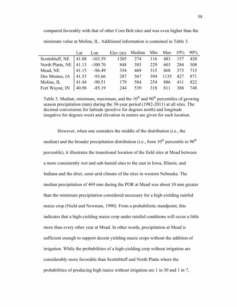
58
compared favorably with that of other Corn Belt sites and was even higher than the
minimum value at Moline, IL. Additional information is contained in Table 3.
Table 3. Median, minimum, maximum, and the 10th and 90th percentiles of growing season precipitation (mm) during the 30-year period (1982-2011) at all sites. The decimal conversions for latitude (positive for degrees north) and longitude (negative for degrees west) and elevation in meters are given for each location.
However, when one considers the middle of the distribution (i.e., the
median) and the broader precipitation distribution (i.e., from 10th percentile to 90th
percentile), it illustrates the transitional location of the field sites at Mead between
a more consistently wet and sub-humid sites to the east in Iowa, Illinois, and
Indiana and the drier, semi-arid climate of the sires in western Nebraska. The
median precipitation of 469 mm during the POR at Mead was about 10 mm greater
than the minimum precipitation considered necessary for a high-yielding rainfed
maize crop (Nield and Newman, 1990). From a probabilistic standpoint, this
indicates that a high-yielding maize crop under rainfed conditions will occur a little
more than every other year at Mead. In other words, precipitation at Mead is
sufficient enough to support decent yielding maize crops without the addition of
irrigation. While the probabilities of a high-yielding crop without irrigation are
considerably more favorable than Scottsbluff and North Platte where the
probabilities of producing high maize without irrigation are 1 in 30 and 1 in 7,
Lat Lon Elev (m) Median Min Max 10% 90% Scottsbluff, NE 41.88 -103.59 1205 274 116 483 157 420 North Platte, NE 41.13 -100.70 848 383 229 603 284 508 Mead, NE 41.15 -96.49 354 469 315 868 373 715 Des Moines, IA 41.53 -93.66 287 567 394 1135 427 871 Moline, IL 41.44 -90.51 179 584 254 886 411 822 Fort Wayne, IN 40.98 -85.19 244 539 318 811 388 748
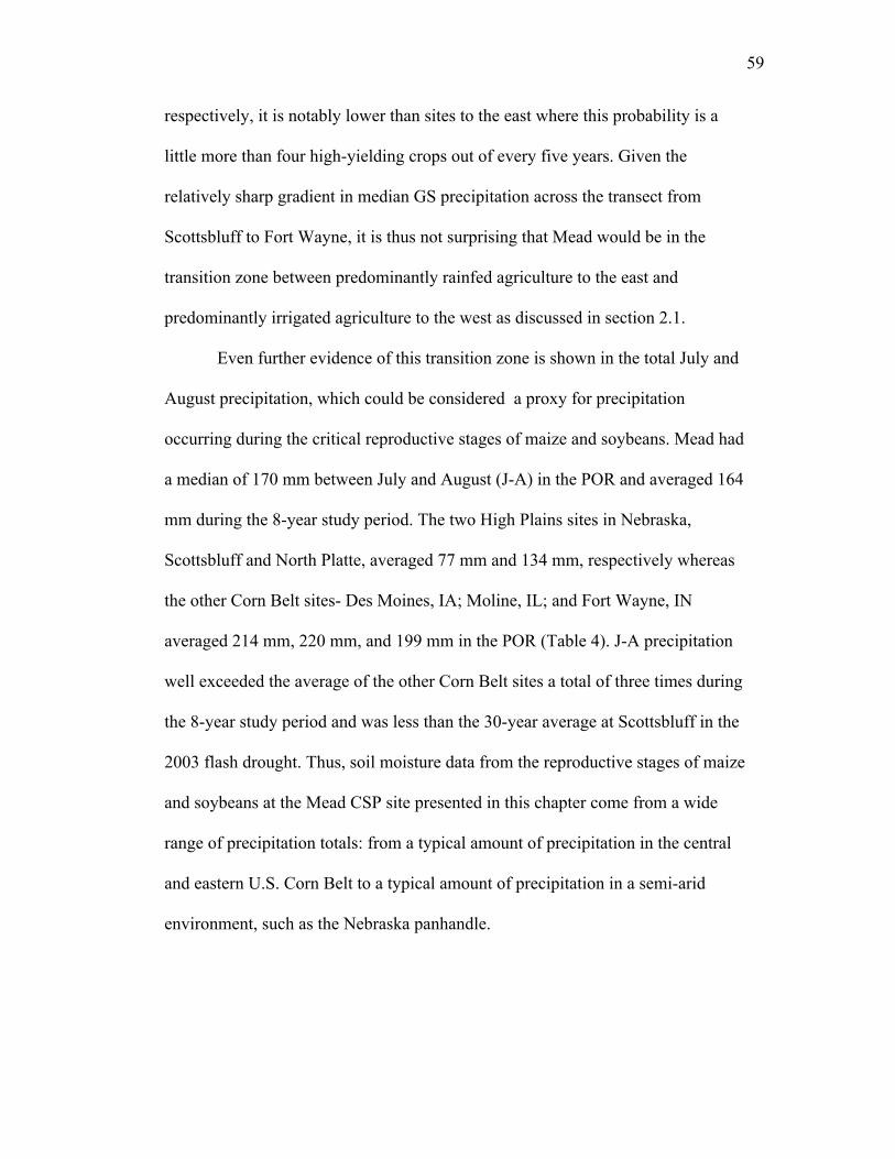
59
respectively, it is notably lower than sites to the east where this probability is a
little more than four high-yielding crops out of every five years. Given the
relatively sharp gradient in median GS precipitation across the transect from
Scottsbluff to Fort Wayne, it is thus not surprising that Mead would be in the
transition zone between predominantly rainfed agriculture to the east and
predominantly irrigated agriculture to the west as discussed in section 2.1.
Even further evidence of this transition zone is shown in the total July and
August precipitation, which could be considered a proxy for precipitation
occurring during the critical reproductive stages of maize and soybeans. Mead had
a median of 170 mm between July and August (J-A) in the POR and averaged 164
mm during the 8-year study period. The two High Plains sites in Nebraska,
Scottsbluff and North Platte, averaged 77 mm and 134 mm, respectively whereas
the other Corn Belt sites- Des Moines, IA; Moline, IL; and Fort Wayne, IN
averaged 214 mm, 220 mm, and 199 mm in the POR (Table 4). J-A precipitation
well exceeded the average of the other Corn Belt sites a total of three times during
the 8-year study period and was less than the 30-year average at Scottsbluff in the
2003 flash drought. Thus, soil moisture data from the reproductive stages of maize
and soybeans at the Mead CSP site presented in this chapter come from a wide
range of precipitation totals: from a typical amount of precipitation in the central
and eastern U.S. Corn Belt to a typical amount of precipitation in a semi-arid
environment, such as the Nebraska panhandle.
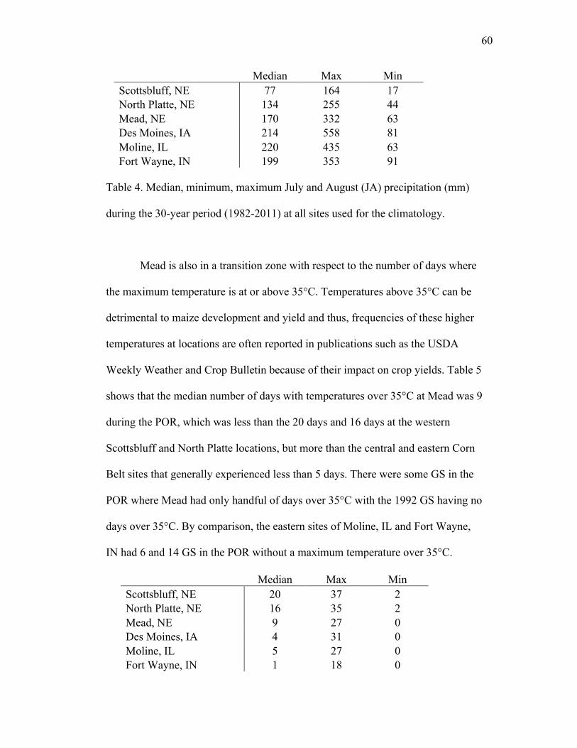
60
Median Max Min
Scottsbluff, NE 77 164 17 North Platte, NE 134 255 44 Mead, NE 170 332 63 Des Moines, IA 214 558 81 Moline, IL 220 435 63 Fort Wayne, IN 199 353 91
Table 4. Median, minimum, maximum July and August (JA) precipitation (mm)
during the 30-year period (1982-2011) at all sites used for the climatology.
Mead is also in a transition zone with respect to the number of days where
the maximum temperature is at or above 35°C. Temperatures above 35°C can be
detrimental to maize development and yield and thus, frequencies of these higher
temperatures at locations are often reported in publications such as the USDA
Weekly Weather and Crop Bulletin because of their impact on crop yields. Table 5
shows that the median number of days with temperatures over 35°C at Mead was 9
during the POR, which was less than the 20 days and 16 days at the western
Scottsbluff and North Platte locations, but more than the central and eastern Corn
Belt sites that generally experienced less than 5 days. There were some GS in the
POR where Mead had only handful of days over 35°C with the 1992 GS having no
days over 35°C. By comparison, the eastern sites of Moline, IL and Fort Wayne,
IN had 6 and 14 GS in the POR without a maximum temperature over 35°C.
Median Max Min
Scottsbluff, NE 20 37 2 North Platte, NE 16 35 2 Mead, NE 9 27 0 Des Moines, IA 4 31 0 Moline, IL 5 27 0 Fort Wayne, IN 1 18 0
61
Table 5. Median, minimum, and maximum number of days in a growing season
during the POR when maximum temperatures equaled or exceeded 35°C.
Precipitation and temperature are both important factors for crop
development and final yield determination. Yet, one issue of using only total GS
precipitation to predict yield is that it does not necessarily reflect the timing of
precipitation during the season. Figure 1 presents accumulated GS precipitation for
all eight seasons at Mead. The wettest GS during the study period occurred in 2007
when maize was the common crop at both field sites, but not have the highest
maize yield at RMS, which was recorded in 2009. The highest maize yield during a
year with significantly less overall GS precipitation than 2007, but the precipitation
was received (as shown in Fig.1) at more regular temporal intervals, and in
somewhat similar amounts. The 2009 GS was also relatively cool (17.9°C versus
the 30-year average of 19.2°C), which when combined with regular rainfall events,
allowed soil moisture to be sustained at higher levels during the critical
reproductive stage compared to 2007.
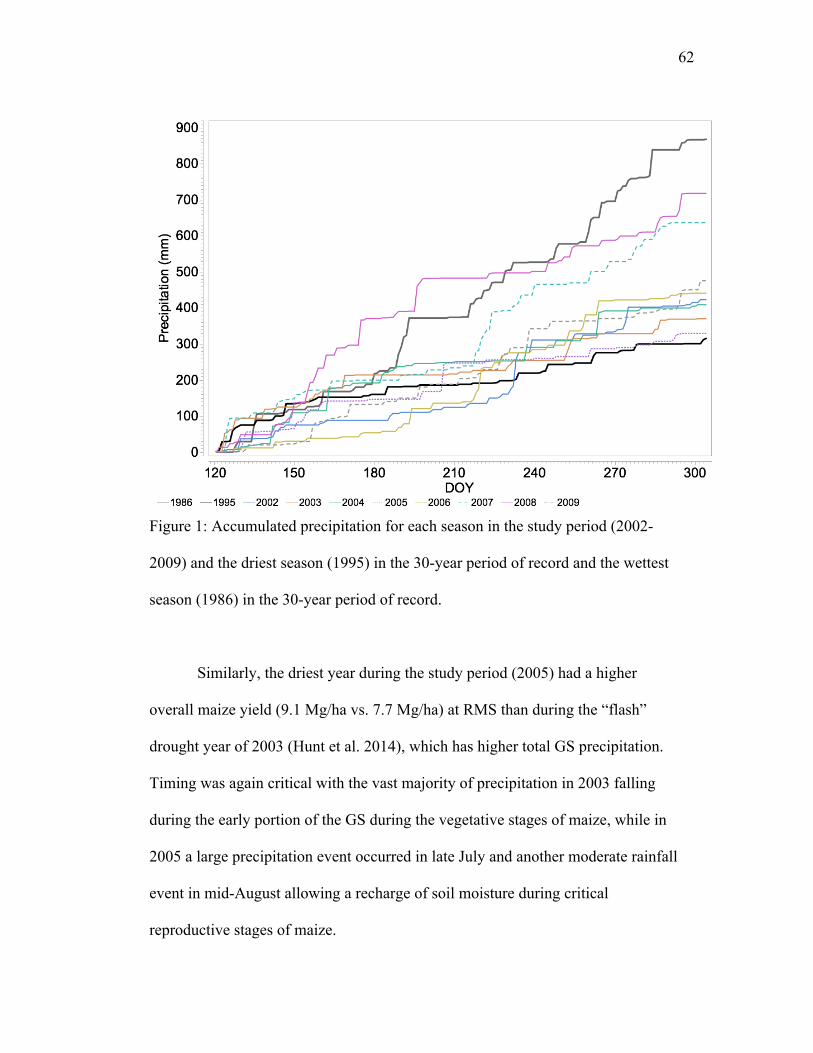
62
Figure 1: Accumulated precipitation for each season in the study period (2002-
2009) and the driest season (1995) in the 30-year period of record and the wettest
season (1986) in the 30-year period of record.
Similarly, the driest year during the study period (2005) had a higher
overall maize yield (9.1 Mg/ha vs. 7.7 Mg/ha) at RMS than during the “flash”
drought year of 2003 (Hunt et al. 2014), which has higher total GS precipitation.
Timing was again critical with the vast majority of precipitation in 2003 falling
during the early portion of the GS during the vegetative stages of maize, while in
2005 a large precipitation event occurred in late July and another moderate rainfall
event in mid-August allowing a recharge of soil moisture during critical
reproductive stages of maize.
63
The previous two paragraphs explained in some detail how varied total GS
precipitation during the study period did not necessarily lead to a direct correlation
with maize yield. The point of the following sections (and this paper in general) is
not for yield prediction or yield correlation based on a few meteorological
variables; rather, the following sections will demonstrate how soil moisture reflects
inter- and intra- seasonal precipitation differences. In the following sections,
shallow depth in-situ soil moisture measurements are shown to be the best
reflection of recent climatic conditions (e.g., hot and dry), and deeper soil moisture
being the best reflection of longer-term (i.e., 30-60 days) climatic conditions.
3.2 Soil Moisture climatology
Table 6 shows general statistics for soil moisture at RMS during the 8-year
study period. As expected, seasonal average water content was lower (higher) in
the GS with lower (higher) precipitation. A comparison of the first and second
halves of the study period demonstrates this clearly. From 2002 through2005, the
average seasonal precipitation was 382 mm and the average water contents were
0.304, 0.331, 0.312, and 0.356 m3/m3 at the10 cm, 25 cm, 50 cm, and 100 cm,
respectively. The 2005 GS was the driest GS overall and had the lowest average
water content at 10 cm and 25 cm depths of any GS in the study period with an
average of 0.285 and 0.304 m3/m3. The lowest average water content at the deeper
depths (i.e., 50 cm and 100 cm) occurred during the 2003 flash drought with an
average of 0.285 and 0.334 m3/m3 at 50 cm and 100 cm respectively. During the
much wetter 2006-2009 period, seasonal precipitation averaged 542 mm and the
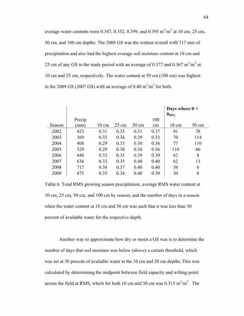
64
average water contents were 0.347, 0.352, 0.399, and 0.395 m3/m3 at 10 cm, 25 cm,
50 cm, and 100 cm depths. The 2008 GS was the wettest overall with 717 mm of
precipitation and also had the highest average soil moisture content at 10 cm and
25 cm of any GS in the study period with an average of 0.377 and 0.367 m3/m3 at
10 cm and 25 cm, respectively. The water content at 50 cm (100 cm) was highest
in the 2009 GS (2007 GS) with an average of 0.40 m3/m3 for both.
Days where θ < θ50%
Season Precip (mm) 10 cm 25 cm 50 cm
100 cm 10 cm 50 cm
2002 423 0.31 0.33 0.31 0.37 91 78 2003 369 0.33 0.36 0.29 0.33 70 114 2004 408 0.29 0.33 0.30 0.36 77 110 2005 329 0.29 0.30 0.36 0.36 110 66 2006 440 0.33 0.35 0.39 0.39 62 8 2007 636 0.33 0.35 0.40 0.40 62 13 2008 717 0.38 0.37 0.40 0.40 36 0 2009 475 0.35 0.34 0.40 0.39 30 0
Table 6. Total RMS growing season precipitation, average RMS water content at
10 cm, 25 cm, 50 cm, and 100 cm by season, and the number of days in a season
when the water content at 10 cm and 50 cm was such that it was less than 50
percent of available water for the respective depth.
Another way to approximate how dry or moist a GS was is to determine the
number of days that soil moisture was below (above) a certain threshold, which
was set at 50 percent of available water at the 10 cm and 50 cm depths. This was
calculated by determining the midpoint between field capacity and wilting point
across the field at RMS, which for both 10 cm and 50 cm was 0.315 m3/m3. The
65
10 cm depth was chosen for further analysis as it had the most dynamic response to
precipitation and incipient dry spells. The 50 cm depth was chosen for analysis as it
was a better indicator of longer-term dry spells than 10 or 25 cm but was more
responsive to short-term precipitation events than at 100 cm. A threshold of 50
percent was selected because this is commonly considered to be the lowest point
where evapotranspiration will equal the potential evapotranspiration rate (Waring
and Running, 1998) and thus is the point where stress due to a lack of soil moisture
could begins to affect the crop.
At 10 cm, the number of days below the threshold ranged from 30 in 2009
to 110 in 2005. The number of days below the threshold at 50 cm followed a
similar pattern with a maximum of 114 days during the 2003 flash drought and 0
days in both 2008 and 2009. Thus, the number of days below the thresholds at 10
cm and 50 cm was much lower in years with precipitation amounts above the long-
term median and much higher during the years where precipitation was much less
than the long-term median. However, total season precipitation was not a perfect
predictor of the number of days below the threshold. Timing of precipitation
played a large role as well. For example, the 2009 GS was not close to being the
wettest year but it had perhaps the most well timed precipitation of any GS in the
study period and was easily the coolest, therefore it had less “stress” than any other
season.
Timing of the precipitation was an important factor influencing soil
moisture conditions. The 2005 GS, though driest, did not have the most days blow
the 50% available water threshold at 50 cm because of the aforementioned timing
66
of significant precipitation events in late July and August. The 2006 GS was very
dry early as shown by Fig. 1 but had fewer days below the threshold than in the
preceding years because of well-timed precipitation in July and August. It could
therefore be argued that timing of precipitation in a GS can be almost, if not
equally, as important as the total amount of GS precipitation. This assertion is
further supported in the remaining subsections.
3.3 Precipitation-Soil Moisture lag
The relationship of precipitation and soil moisture was strong when
considering the study period in its entirety, with an R2 of 0.79 between total
precipitation and mean water content over all depths at RMS. But as previous
studies documented [e.g., Basara et al. (1998); Illston and Basara (2003)], flash
droughts can occasionally occur in GSwith above average precipitation and
excessively high temperatures and drying conditions, which can cause severe
agricultural impacts. Thus, the timing of precipitation is critical and total GS
precipitation may not necessarily reflect a prolonged stretch of dry weather that
occurred during a portion of the GS.
Even though precipitation and soil moisture were strongly correlated over
the study period, the relationship weakened when comparing mean water content
of all soil depths and precipitation over shorter-time scales (e.g., a few weeks)
within a GS. This implies that a lag existed between precipitation and soil moisture
during the eight years of the study period. To test this, we considered the water
content on a given date (e.g., 1 August) and compared it to the previous 14-, 30-,
67
and 60-day precipitation totals to test both the lag and varying time scales of the
precipitation-soil moisture lags at varying soil depths.
Table 7 shows that the correlation between soil moisture and precipitation
across the GS. In general, strongest relationship was found during the hotter
months of July of August with the highest correlations between short-term (i.e.,
14-day) precipitation and soil moisture at shallower depths and medium- and
longer-term precipitation and deeper soil moisture conditions. This illustrates the
tendency for shallow soil moisture to be most affected by short-term dry spells or a
single precipitation event and deeper soil moisture to depict the antecedent
precipitation conditions on the order of a month(s).
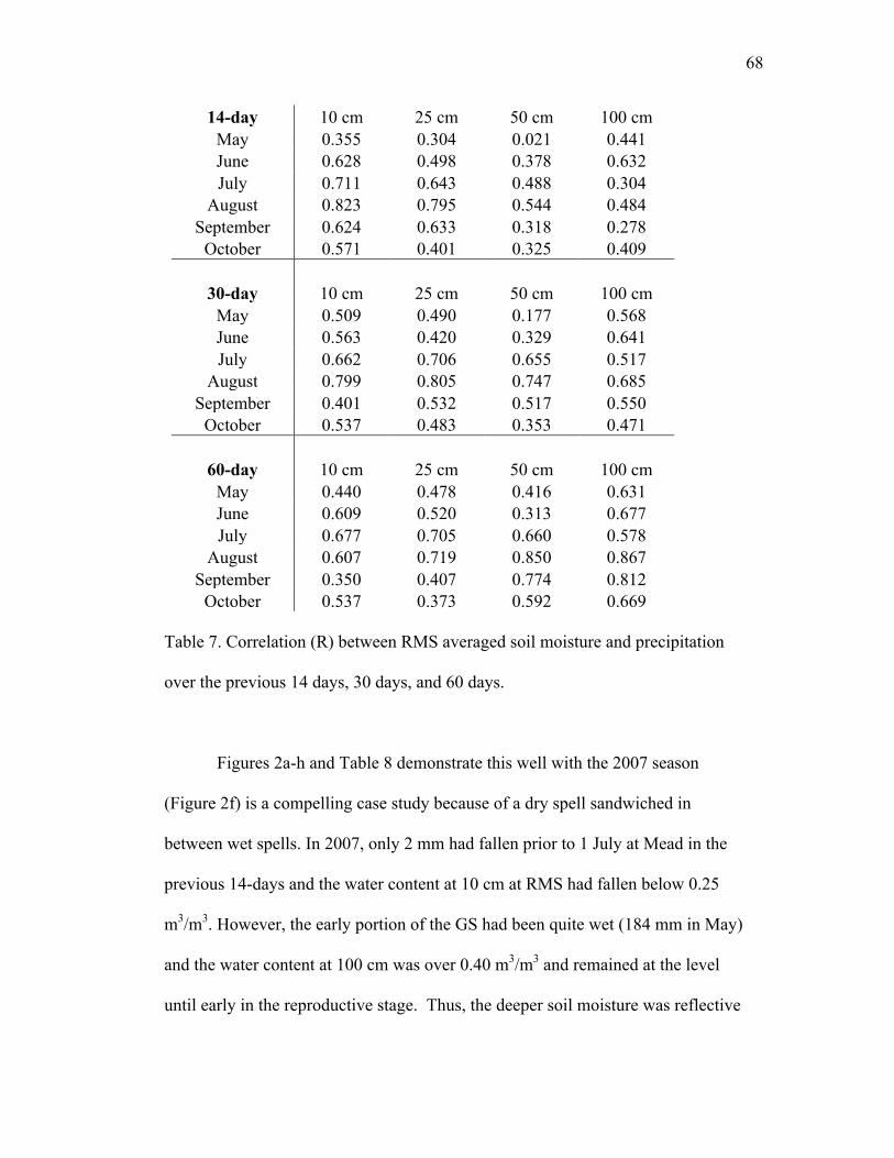
68
14-day 10 cm 25 cm 50 cm 100 cm May 0.355 0.304 0.021 0.441 June 0.628 0.498 0.378 0.632 July 0.711 0.643 0.488 0.304
August 0.823 0.795 0.544 0.484 September 0.624 0.633 0.318 0.278
October 0.571 0.401 0.325 0.409
30-day 10 cm 25 cm 50 cm 100 cm May 0.509 0.490 0.177 0.568 June 0.563 0.420 0.329 0.641 July 0.662 0.706 0.655 0.517
August 0.799 0.805 0.747 0.685 September 0.401 0.532 0.517 0.550
October 0.537 0.483 0.353 0.471
60-day 10 cm 25 cm 50 cm 100 cm May 0.440 0.478 0.416 0.631 June 0.609 0.520 0.313 0.677 July 0.677 0.705 0.660 0.578
August 0.607 0.719 0.850 0.867 September 0.350 0.407 0.774 0.812
October 0.537 0.373 0.592 0.669
Table 7. Correlation (R) between RMS averaged soil moisture and precipitation
over the previous 14 days, 30 days, and 60 days.
Figures 2a-h and Table 8 demonstrate this well with the 2007 season
(Figure 2f) is a compelling case study because of a dry spell sandwiched in
between wet spells. In 2007, only 2 mm had fallen prior to 1 July at Mead in the
previous 14-days and the water content at 10 cm at RMS had fallen below 0.25
m3/m3. However, the early portion of the GS had been quite wet (184 mm in May)
and the water content at 100 cm was over 0.40 m3/m3 and remained at the level
until early in the reproductive stage. Thus, the deeper soil moisture was reflective

69
of the wet spring while the shallow soil moisture was reflective of the dryness of
the previous few weeks. Significant precipitation returned in early August and
immediately brought the field-average water content at 10 cm from 0.21 m3/m3 to
0.39 m3/m3 over the course of five days. There was also recharge observed at 50
cm and then at 100 cm after the five day wet spell, but the 10 cm depth was
certainly more reflective of the short-term wet spell than the deeper depths.
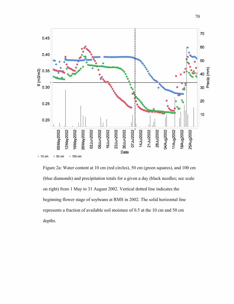
70
Figure 2a: Water content at 10 cm (red circles), 50 cm (green squares), and 100 cm
(blue diamonds) and precipitation totals for a given a day (black needles; see scale
on right) from 1 May to 31 August 2002. Vertical dotted line indicates the
beginning flower stage of soybeans at RMS in 2002. The solid horizontal line
represents a fraction of available soil moisture of 0.5 at the 10 cm and 50 cm
depths.
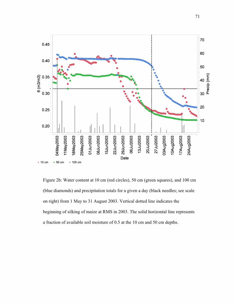
71
Figure 2b: Water content at 10 cm (red circles), 50 cm (green squares), and 100 cm
(blue diamonds) and precipitation totals for a given a day (black needles; see scale
on right) from 1 May to 31 August 2003. Vertical dotted line indicates the
beginning of silking of maize at RMS in 2003. The solid horizontal line represents
a fraction of available soil moisture of 0.5 at the 10 cm and 50 cm depths.
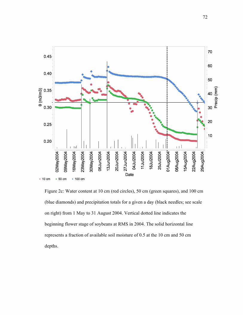
72
Figure 2c: Water content at 10 cm (red circles), 50 cm (green squares), and 100 cm
(blue diamonds) and precipitation totals for a given a day (black needles; see scale
on right) from 1 May to 31 August 2004. Vertical dotted line indicates the
beginning flower stage of soybeans at RMS in 2004. The solid horizontal line
represents a fraction of available soil moisture of 0.5 at the 10 cm and 50 cm
depths.
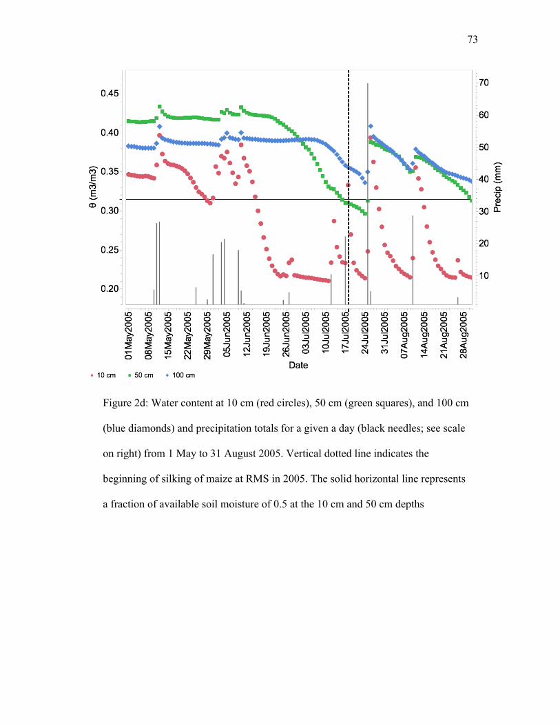
73
Figure 2d: Water content at 10 cm (red circles), 50 cm (green squares), and 100 cm
(blue diamonds) and precipitation totals for a given a day (black needles; see scale
on right) from 1 May to 31 August 2005. Vertical dotted line indicates the
beginning of silking of maize at RMS in 2005. The solid horizontal line represents
a fraction of available soil moisture of 0.5 at the 10 cm and 50 cm depths
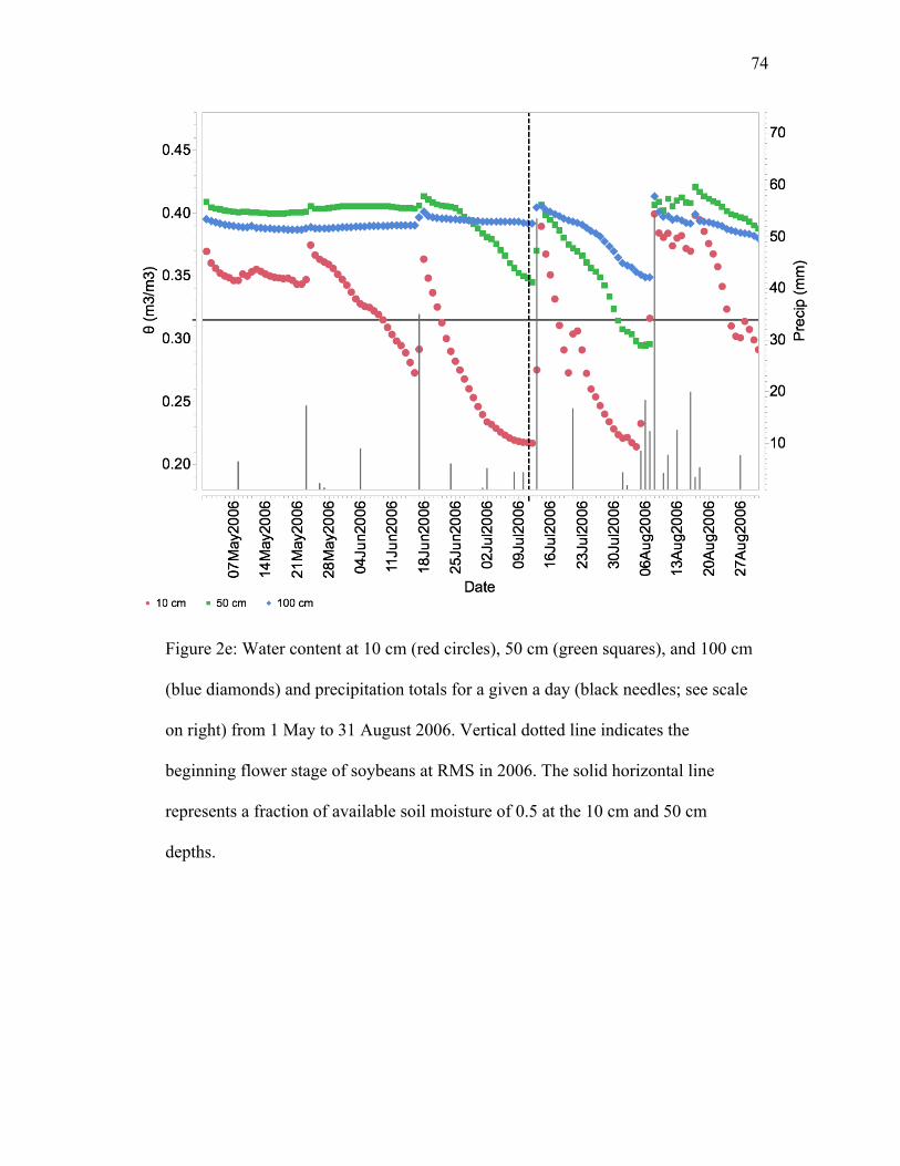
74
Figure 2e: Water content at 10 cm (red circles), 50 cm (green squares), and 100 cm
(blue diamonds) and precipitation totals for a given a day (black needles; see scale
on right) from 1 May to 31 August 2006. Vertical dotted line indicates the
beginning flower stage of soybeans at RMS in 2006. The solid horizontal line
represents a fraction of available soil moisture of 0.5 at the 10 cm and 50 cm
depths.
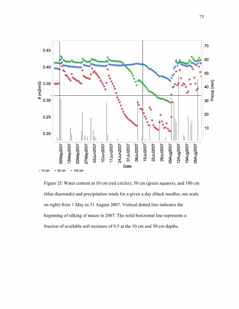
75
Figure 2f: Water content at 10 cm (red circles), 50 cm (green squares), and 100 cm
(blue diamonds) and precipitation totals for a given a day (black needles; see scale
on right) from 1 May to 31 August 2007. Vertical dotted line indicates the
beginning of silking of maize in 2007. The solid horizontal line represents a
fraction of available soil moisture of 0.5 at the 10 cm and 50 cm depths.
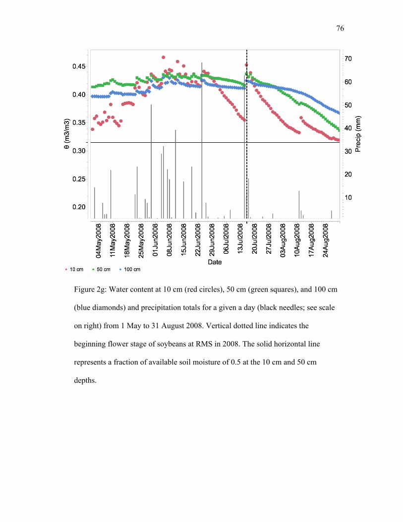
76
Figure 2g: Water content at 10 cm (red circles), 50 cm (green squares), and 100 cm
(blue diamonds) and precipitation totals for a given a day (black needles; see scale
on right) from 1 May to 31 August 2008. Vertical dotted line indicates the
beginning flower stage of soybeans at RMS in 2008. The solid horizontal line
represents a fraction of available soil moisture of 0.5 at the 10 cm and 50 cm
depths.
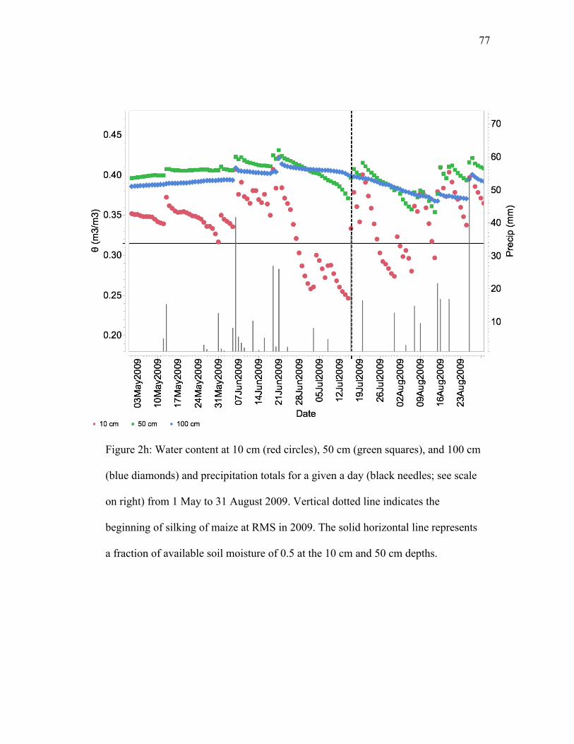
77
Figure 2h: Water content at 10 cm (red circles), 50 cm (green squares), and 100 cm
(blue diamonds) and precipitation totals for a given a day (black needles; see scale
on right) from 1 May to 31 August 2009. Vertical dotted line indicates the
beginning of silking of maize at RMS in 2009. The solid horizontal line represents
a fraction of available soil moisture of 0.5 at the 10 cm and 50 cm depths.
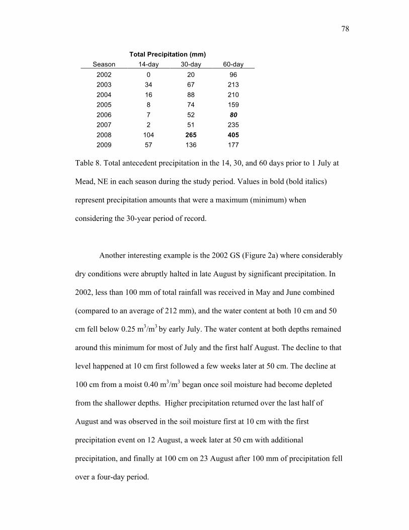
78
Total Precipitation (mm) Season 14-day 30-day 60-day
2002 0 20 96 2003 34 67 213 2004 16 88 210 2005 8 74 159 2006 7 52 80 2007 2 51 235 2008 104 265 405 2009 57 136 177
Table 8. Total antecedent precipitation in the 14, 30, and 60 days prior to 1 July at
Mead, NE in each season during the study period. Values in bold (bold italics)
represent precipitation amounts that were a maximum (minimum) when
considering the 30-year period of record.
Another interesting example is the 2002 GS (Figure 2a) where considerably
dry conditions were abruptly halted in late August by significant precipitation. In
2002, less than 100 mm of total rainfall was received in May and June combined
(compared to an average of 212 mm), and the water content at both 10 cm and 50
cm fell below 0.25 m3/m3 by early July. The water content at both depths remained
around this minimum for most of July and the first half August. The decline to that
level happened at 10 cm first followed a few weeks later at 50 cm. The decline at
100 cm from a moist 0.40 m3/m3 began once soil moisture had become depleted
from the shallower depths. Higher precipitation returned over the last half of
August and was observed in the soil moisture first at 10 cm with the first
precipitation event on 12 August, a week later at 50 cm with additional
precipitation, and finally at 100 cm on 23 August after 100 mm of precipitation fell
over a four-day period.
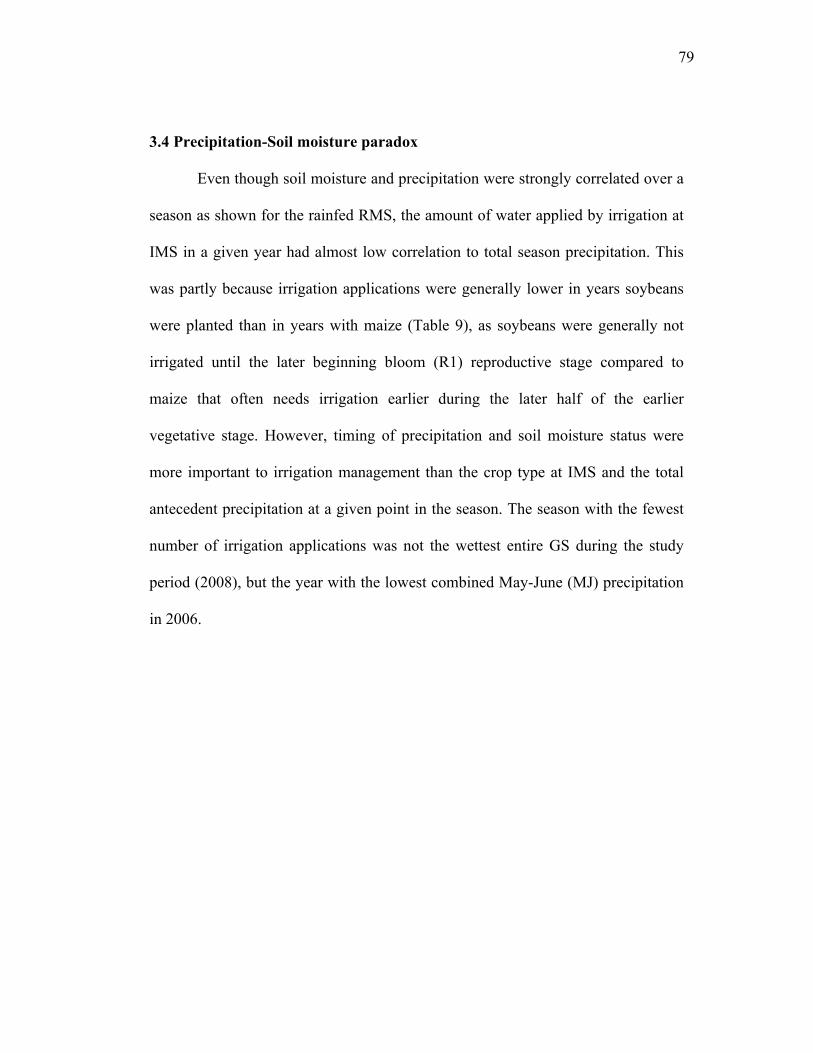
79
3.4 Precipitation-Soil moisture paradox
Even though soil moisture and precipitation were strongly correlated over a
season as shown for the rainfed RMS, the amount of water applied by irrigation at
IMS in a given year had almost low correlation to total season precipitation. This
was partly because irrigation applications were generally lower in years soybeans
were planted than in years with maize (Table 9), as soybeans were generally not
irrigated until the later beginning bloom (R1) reproductive stage compared to
maize that often needs irrigation earlier during the later half of the earlier
vegetative stage. However, timing of precipitation and soil moisture status were
more important to irrigation management than the crop type at IMS and the total
antecedent precipitation at a given point in the season. The season with the fewest
number of irrigation applications was not the wettest entire GS during the study
period (2008), but the year with the lowest combined May-June (MJ) precipitation
in 2006.
80
Season Crop Type Precipitation (mm) Irr. Treatments Irrigation (mm)
2002 S 423 6 209 2003 M 369 11 347 2004 S 408 5 159 2005 M 329 9 302 2006 S 440 4 122 2007 M 636 8 265 2008 S 717 7 251 2009 M 475 6 198
Table 9. Total growing season precipitation (mm) at RMS, the number of irrigation
treatments, and total irrigation amount applied (mm) over the eight growing
seasons at IMS. For crop type, S= soybeans and M= maize.
This paradox is best explained with some background about these two
highlighted GS. The 2006 GS had the driest start (i.e., MJ period) in the POR and
the 2008 GS was the wettest (refer to Fig. 1). Overall, precipitation in 2006 was a
little below the median, while 2008 was one of the wettest GS in the POR. It would
typically be assumed that the amount of water applied by irrigation in 2006 would
far be exceeded the amount applied in 2008. However, the opposite was true with
the2006 GS having the fewest irrigation applications of any year in the study
period, while the 2008 season had the most irrigation applications of any year
planted to soybeans, including the 2002 drought year.
Figure 2e shows these differences between these two years for the IMS.
During the 2006 GS, timely precipitation in July prevented significant depletion at
the deeper the 50 cm and 100 cm depths at both RMS and IMS. Then, frequent
81
precipitation in August allowed for significant moistening at all depths at RMS and
negated the necessity of frequent irrigation applications at IMS.
Conversely, the only dry spell during the entire 2008 GS occurred during a
critical time (i.e., August) for soybeans. Even though the dry spell did not lead to a
significant decline in soil moisture at 50 cm and 100 cm, the depletion of soil
moisture in the shallow part of the profile necessitated the need for irrigation
treatments, as there were concerns about root depths potentially being more
shallow than normal because of the abnormally wet spring. Thus, frequent
irrigation applications were necessary in 2008, in spite of the wet GSoverall.
4.0 Summary and Conclusions
Eight years of soil moisture and climatological data from the CSP at Mead,
NE revealed unique results from a location situated in a transition zone between
predominantly rainfed agriculture to the east and predominantly irrigated
agriculture to the west. The eight years at Mead featured total precipitation for May
and June in 2008 that would have been the wettest common period at the Eastern
Corn Belt site of Fort Wayne, IN. It also featured total precipitation for July and
August in 2003 that was lower than the common period average at the semi-arid,
western High Plains site of Scottsbluff, NE. Thus, climatological extremes for both
the wet end and dry conditions across this broader east-west expanse across the
U.S. Great Plains and Corn Belt were realized at Mead during the eight-year study
period, even though the average precipitation during the study period at Mead was
close to the 30-year median.
82
During the first half of the study period (2002-2005), there were prolonged
periods in all four GS where the soil moisture content was below the 50 percent of
available water threshold at both 10 cm and 50 cm depths. This lack of root-zone
soil moisture had a detrimental impact on yields at the rainfed site (RMS)
compared to the irrigated site (IMS), especially during the flash drought of 2003
when the maize yield at RMS was less than half of the IMS. These four early GS
demonstrated the benefit of having irrigation at Mead and the necessity of it in a
semi-arid environment where GS conditions are typically like those in the first half
of the study period in this research.
Conversely, the latter half of the study period was generally wetter than
average. Precipitation at Mead was not only higher in sum over those years, but
was also more regularly distributed, resulting in the average soil moisture content
being much higher than the earlier part of the study period. Drier periods did occur
in the second half of the study period and soil moisture stress was expressed in the
top depth, but typically had minimal effects on the deeper depths. The magnitude
of stress tended to be lower and the duration much shorter during these years. As a
result, irrigation treatments were less numerous at IMS and yields at RMS were
closer to those of IMS, particularly in 2009 (maize) when there were no days of
stress at 50 cm and in 2006 when significant precipitation was well-timed during
the reproductive cycle of the soybean crop.
The results obtained during this study period showed the importance of the
timing of precipitation and soil moisture response, particularly for irrigation
scheduling at IMS. The years with the fewest irrigation application for both maize
83
and soybeans were not the wettest years during the study period. Paradoxically, the
year with the fewest irrigation treatments when soybeans were the common crop
between RMS and IMS was in 2006, which had below average GS precipitation.
The year with the most irrigation treatments when soybeans were also the common
crop in 2008 was one of the wettest seasons in the 30-year POR. The primary
difference between the below average 2006 GS and the wet 2008 GS was that
precipitation fell at regular intervals during critical reproductive stages for
soybeans in 2006 keeping the soil profile moist. Conversely, the only dry spell of
the 2008 GS occurred during that same critical period, thus necessitating irrigation
applications that prevented depletion of the top half of the soil profile at IMS.
For GS where maize was the common crop, the wettest GS (2007) did not
have the highest averaged soil moisture or the highest yields at RMS. That
distinction belonged to the 2009 GS, which was only slightly above the 30-year
median. Again, timing of the rains was the key difference with a large share of the
precipitation occurring early in the season for 2007 and again late in the summer
and autumn. Both of these time spans were outside the critical reproductive period
for maize that determines the crop’s final yield. During the 2009 GS, most rainfall
occurred during these critical stages for maize, keeping the soil profile moist and
achieving higher yields than might be expected when total annual precipitation was
only slightly above the 30-year median. Thus, the old adage that timing is
everything, certainly has a strong element of truth to it when it comes to
precipitation, soil moisture, and crop production in this study.
84
As shown and discussed previously in this chapter, soil moisture under crop
cover is highly dependent on the amount of precipitation. Soil moisture, on
average, was higher at all depths in the later years of the study when precipitation
was more plentiful. Timing of precipitation was important too and as in the case of
the 2007 and 2008 growing seasons, abnormally wet seasons can have dry spells
long enough in duration to require a number of irrigation treatments, particularly if
the only dry spell in a season coincides with the most critical time for a crop. In
areas where irrigation is a necessity for high-yielding crops and groundwater
resources are becoming more limited, knowledge of soil moisture allows producers
to make smart decisions about when to irrigate.
For example, knowing the crop could go another few days before an
irrigation could save a lot of money and water if the decision to wait a few days
based on soil moisture data if a significant precipitation event materialized. Soil
moisture is not perfectly correlated with crop yield, because other external factors
(i.e., non-agroclimatological) can have a significant impact. However, soil
moisture data can help fill in the knowledge gap as to the effectiveness of
precipitation events and if assimilated properly into crop models or land models
coupled with crop models, it is quite likely that uncertainty in yield projections
could be reduced.
85
5.0 Acknowledgements:
The research presented here was supported by the Office of Science (BER),
U.S. Department of Energy Grant (No. DE-FG02-03ER63639 and the University
of Nebraska-Lincoln Program of Excellence. Special thanks to Todd Schimelfenig,
Dave Scoby, and Glen Roebke for providing technical expertise and data.
6.0 References:
Basara, J.B., Arndt, D.S., Johnson, H.L., Brotzge, J.G., Crawford, K.C., 1998: An
analysis of the drought of 1998 using the Oklahoma Mesonet. EOS Trans., AGU,
79, 258.
Calvino, P.A., Andrade, F.H., Sadras, V.O., 2003. Maize yield as affected by water
availability, soil depth, and crop management. Agron. J. 95, 275-281.
Chapman, S.S., Omernik, J.M., Freeouf, J.A., Huggins, D.G., McCauley, J.R.,
Freeman, C.C., Steinauer, G., Angelo, G.T., and Schlepp, R.L. 2001. Ecoregions of
Nebraska and Kansas. U.S. Geological Survey, Reston, VA. Scale 1:1,950,000.
Cosby, B.J., Hornberger, G.M., Clapp, R.B., Ginn, T.R., 1984. A statistical
exploration of the relationships of soil moisture characteristics to the physical
properties of soils. Water Resour. Res. 20, 682-690.
Doss, B.D., Pearson, R.W., Rogers, H.T. 1974. Effect of soil moisture stress at
various growth stages on soybean yield. Agron. J. 66, 297-299.
86
Earl, H. J., Davis, R. F., 2003. Effect of drought stress on leaf and whole canopy
maize radiation use efficiency and yield of maize. Agron. J. 95, 688-696.
Eck, H.V., Mathers, A.C., Musick, J.T. 1987. Plant water stress at various growth
stages and growth and yield of soybeans. Field Crops Res. 17, 1-16.
Ek, M.B., Mitchell, K.E., Lin Y., Rogers, E., Grunmann, P., Koren,V., Gayno, G.,
Tarpley, J.D. 2003. Implementation of Noah land surface model advances in the
National Centers for Environmental Prediction operational mesoscale Eta model, J.
Geophys. Res. 108(D22), 8851, doi:10.1029/2002JD003296.
Gutmann, E.D., Small, E.E. 2005. The effect of soil hydraulic properties vs. soil
texture in land surface models. Geophys. Res. Lett., 32, doi:
10.1029/2004GL021843.
Harrison, K.W., Kumar, S.V., Peters-Lidard, C.D., Santanello, J.A. 2012.
Quantifying the change in soil moisture modeling uncertainty from remote sensing
observations using Bayesian inference. Water Resour. Res., 48, W11514,
doi:10.1029/2012WR012337.
Hollinger, S. E., Isard, S. A. 1994. A soil moisture climatology of Illinois. J.
Climate 7, 822-833.

87
Hubbard, K.G., You, J., Sridhar,V., Hunt, E., Korner,.S., Roebke, G., 2009. Near-
surface soil moisture monitoring for water resources management on a wide-area
basis in the Great Plains, Great Plains Res., 19, 45-54.
Hunt, E. D., Hubbard, K. G., Wilhite, D.A., Arkebauer, T.J., Dutcher, A.L., 2009.
The development and evaluation of a soil moisture index. Int. J. Climatol. 29, 747-
759.
Hunt, E.D., Svoboda, M., Wardlow, B., Hubbard, K., Hayes, M., Arkebauer, T.
2014. Monitoring the effects of rapid onset of drought on non-irrigated maize with
agronomic data and climate-based drought indices. Agric. For. Meteorol. 191, 1-
11.
Illston, B.G., Basara, J.B., 2003. Analysis of short-term droughts in Oklahoma.
Eos. Trans. AGU: 84 (17), 157.
Illston, B.G., Basara, J. B., Crawford, K.C., 2004. Seasonal to interannual
variations of soil moisture measured in Oklahoma. Int. J. Climatol., 24, 1883-
1896.
Kumar, S. V., Peters-Lidard, C. D., Tian, Y., Houser, P. R., Geiger, J., Olden, S.,
Lighty, L., Eastman, J. L., Doty, B., Dirmeyer, P., Adams, J., Mitchell, K., Wood,
88
E. F., Sheffield, J., 2006. Land Information System - An Interoperable Framework
for High Resolution Land Surface Modeling, Environ. Model. Soft. 21, 1402-1415.
Kumar, S.V., Reichle, R.H., Peters-Lidard, C.D., Koster, R.D., Zhan, X.W., Crow,
W.T., Eylander, J.B., Houser, P.R., 2008. A land data surface assimilation
framework using the land information system: Description and applications, Adv.
Water Resourc., 31,1419-1432.
Kumar, S., Reichle, R. H., Harrison, K. W., Peters-Lidard, C. D., Yatheendradas,
S., Santanello., J. A., 2012. A comparison of methods for a priori bias correction in
soil moisture data assimilation, Water Resour. Res., 48, W09305.
Meyer, S.J., Hubbard, K.G., Wilhite, D.A., 1993. The development of a crop-
specific drought index corn. I. Agron. J. 85: 388-395.
Nghiem, S.V.,Wardlow, B.D., Allured, D., Svoboda, M.D., LeComte, D.,
Rosencrans, M., Chan, S.K., Neumann, G., 2012. Microwave remote sensing of
soil moisture: Science and applications. In Remote Sensing of Drought: Innovative
Monitoring Approaches, eds. B.D. Wardlow, M.C. Anderson, and J.P. Verdin.
Boca Raton, FL: CRC Press.
89
Nield, R.E., Newman, J.E., 1990. Growing season characteristics and requirements
in the Corn Belt. National Corn Handbook, Purdue University, Cooperation
Extension Service, West Lafayette, IN.
Nielsen, D.C., Halvorson, A.D., Vigil, M.E., 2010. Critical precipitation period for
dryland maize production. Field Crops Res. 118, 259-263.
Peters-Lidard, C. D., Houser, P.R., Tian, Y., Kumar, S.V., Geiger, J., Olden, S.,
Lighty, L., Doty, B., Dirmeyer, P., Adams, J., Mitchell, K., Wood, E.F., Sheffield,
J. 2007. High-performance Earth system modeling with NASA/GSFC's Land
Information System. Innovations in Systems and Software Engineering. 3, 157-
165.
Santanello, J. A., Peters-Lidard, C., Garcia, M., Mocko, D., Tischler, M., Moran,
M. S., Thoma, D.P. 2007. Using Remotely-Sensed Estimates of Soil Moisture to
Infer Spatially Distributed Soil Hydraulic Properties. Remote Sensing Environ.
110, 79-97.
Saxton, K.E., Rawls, W.J., 2006. Soil moisture characteristic estimates by texture
and organic matter for hydrologic solutions. Soil Sci. Am. J. 70, 1569-1578.
Scott, R.W., Krug, E.C., Burch, S.L., 2010. Illinois soil moisture under sod
experiment. J. Hydrometeor. 11, 683-704.
90
Sophocleous, M., 2012. Conserving and extending the useful life of the largest
aquifer in North America: The future of the High Plains/Ogallala Aquifer.
Groundwater, 50, 831-839.
Suyker, A.E., Verma, S.B., Burba, C.G. 2003. Interannual variability in net CO2
exchange of a native tallgrass prairie. Global Change Biol. 9, 1-11.
Suyker, A.E., Verma, S.B., Burba, G.G., Arkebauer, T.J., Walters, D.T., Hubbard,
K.G., 2004. Growing season carbon dioxide exchange in irrigated and rainfed
maize, Agric. For. Meteorol. 124, 1-13.
Suyker, A. E., Verma, S.B., 2008. Interannual water vapor and energy exchange in
an irrigated maize-based agroecosystem. Agricul. For. Meteorol. 148, 417-427.
Suyker, A. E., Verma, S.B., 2009. Evapotranspiration of irrigated and rainfed
maize-soybean cropping systems. Agricul. For. Meteorol. 149, 443-452.
Suyker, A.E., Verma, S.B., 2012. Gross primary production and ecosystem
respiration of irrigated and rainfed maize-soybean cropping system over 8 years.
Agric. For. Meteorol. 165, 12-24.
Topp, G.C., Davis, J.L., Annan, A.P., 1980. Electromagentic determination of soil
moisture content: measurement in coaxial transmission lines. Water Resourc. Res.,
16, 574-582.
91
Verma, S.B., Dobermann, A., Cassman, K.G., Walters, D.T., Knops, J.M.,
Arkebauer, T.J., Suyker, A.E., Burba, G.G., Amos, B., Yang, H., Ginting, D.,
Hubbard, K.G., Gitelson, A.A., Walter-Shea, E.A., 2005. Annual carbon dioxide
exchange in irrigated and rainfed maize-based agroecosystems. Agricul. For.
Meteorol. 131, 77-96.
Vinnikov, K.Y., Robock, A., Qiu, S., Entin, J.K., Owe, M., Choudhury, B.J.,
Hollinger, S.E., Njoku, E.G., 1999. Satellite remote sensing of soil moisture in
Illinois, United States. J. Geophys. Res. 104, 4145-4168.
Waring, R.H., Running, S.W., 1998. Forest Ecosystems: Analysis at Multiple
Scales. Academic Press, New York.
You, J., Hubbard, K.G., Mahmood, R., Sridhar, V., Todey, D. 2010. Quality
control of soil moisture data in Applied Climate Information System - case study in
Nebraska. J. Hydrol. Engineer. 15, 200-209.

92
CHAPTER 3: THE DYNAMIC RELATIONSHIP BETWEEN SOIL MOISTURE AND BIOPHYSICAL MEASUREMENTS
Abstract: The purpose of this chapter is to show the relationship between in-situ soil moisture from
a rainfed field and biophysical measurements at a rainfed and nearby irrigated field. Soil
moisture sensors were installed at four depths (10 cm, 25 cm, 50 cm, and 100 cm) in
Intensive Management Zones (IMZ's) for the purpose of determining crucial plant-soil
water relationships under maize and soybeans, both irrigated and rainfed, as part of the
Carbon Sequestration Project (CSP) at Mead, NE. The eight years (2002-2009) of soil
moisture data utilized in this study captured a range of different growing season
conditions, from drought and flash drought to significantly above-average precipitation.
This chapter shows that biophysical measurements, such as evapotranspiration and gross
primary productivity, had a dynamic response to soil moisture. During the drier seasons,
this chapter shows evidence that implies stomatal conductance was negatively affected by
soil water stress with direct comparisons of evapotranspiration and gross primary
productivity at the irrigated and rainfed field. Ten-day averaged ratios of available energy
partitioned to latent heat between the rainfed and irrigated field showed that the rainfed
field was sensitive to moderate levels of water stress during peak photosynthesis potential
(i.e., the midday hours) and was sensitive to high levels of water stress during the entire
day during periods of water stress. This chapter also demonstrates that timing of
precipitation is crucial and that above average precipitation in a season doesn’t preclude
periods of soil water stress if a dry period is sandwiched between wet periods.
93
1.0 Introduction
This chapter presents unique results obtained from eight years of soil water
and biophysical measurements under a rainfed and irrigated agroecosystem. Soil
water is an integral part of the hydrologic cycle and a critical parameter for plant
growth and development. The previous chapter in the series demonstrated the
importance and the growing demand for in-situ soil water measurements.
Biophysical measurements, such as evapotranspiration, are an important link
between soil moisture and the lower boundary layer of the atmosphere. That link
between soil moisture and biophysical measurements under crop cover is the focus
of this chapter.
Since its inception in 2001, research from the ongoing CSP at Mead, NE
has made outstanding contributions to the understanding of carbon and energy
balance over irrigated and rainfed maize and soybeans. In Suyker et al. (2004), the
authors presented results of net ecosystem CO2 exhange (NEE) and gross primary
productivity (GPP) during the first year (2001) of the CSP. A dry and hot spell in
the middle of that growing season reduced leaf area index (LAI) and NEE at the
rainfed maize soybean rotation (RMS) compared to the irrigated maize soybean
rotation (IMS).
Verma et al. (2005) reported that GPP was almost twice as high in a maize
season as in a soybean season and that net ecosystem production (NEP) was about
the same in the rainfed and irrigated field, as increased respiration in irrigated
fields with higher soil moisture offset the higher GPP at the irrigated sites
compared to RMS. Suyker and Verma (2009) showed that growing season ET
94
accounted for an average of 84 and 72 percent of the annual evaporation at the
irrigated sites (ICM, IMS) and RMS respectively. As expected, annual ET was
higher at the irrigated sites than at RMS, particularly during the flash drought that
occurred during the 2003-2004 season, and was higher in maize years than in
soybean years at both IMS and RMS. The authors also showed that the crop
coefficient (Kc), which is calculated as the ratio of ET to reference ET (ETo), was
as much as 30 percent higher at IMS than at RMS during the middle of the 2003
flash drought.
Suyker and Verma (2010) showed that the seasonal distributions of GPP
were consistent in maize and soybeans throughout the six seasons and that GPP
was consistently higher in the irrigated fields than at IMS. This was especially true
in the 2003 growing season when cumulative GPP was reduced by 24 percent at
RMS compared to IMS. Suyker and Verma (2012) further added that green leaf
LAI was a dominant factor in explaining interannual variability of GPP in maize.
As also shown in earlier results, mean annual GPP of soybeans was significantly
less than that of maize (Suyker and Verma 2010).
The CSP is comprised of three field sites under three distinct cropping
systems: 1) irrigated, continuous maize, 2) an irrigated, maize-soybean rotation,
and 3) a rainfed maize-soybean rotation. Each field has multiple intensive
management zones (IMZ’s) where soil water, soil temperature, and other
agroecological variables are measured. Soil water, ET, and GPP are among the
state variables measured hourly during the eight years (2002-2009) of this study.
95
2.0 Materials and methods
2.1. Carbon Sequestration Project study site
The CSP is located at the University of Nebraska-Lincoln (UNL)
Agricultural Research and Development Center in Saunders County, Nebraska near
the town of Mead. This location is roughly 35 km northeast of Lincoln, NE and is
defined in Chapman et al. (2001) as being at the western edge of the Western Corn
Belt Plains ecoregion. As discussed in Hunt et al (in press), the Mead CSP study
site is situated in an area that is a sharp transition zone from predominantly rainfed
to predominantly irrigated agroecosystems. Maize and soybeans are the main crops
grown in the area.
The CSP commenced in the spring of 2001 and consists of three sites. The
first agroecosystem is an irrigated, continuous maize (ICM) site centered at
41˚09’54.2” N, 96˚ 28’35.9” W with an irrigated area of 48.7 ha. The second
agroecosystem is an irrigated, rotated maize-soybean (IMS) site centered at
41˚09’53.5” N, 96˚ 28’12.3” W with an irrigated area of 52.4 ha. Both ICM and
IMS were irrigated rotations of maize and soybeans under no-till in the ten years
prior to the initialization of the CSP. The third agroecosystem is a rainfed, rotated
maize-soybean (RMS) site centered at 41˚10’46.8” N, 96˚ 26’22.7” W with an area
of 65.4 ha. Prior to the CSP, RMS had 2-4 ha plots of maize, soybeans, wheat, and
oats with tillage (Verma et al. 2005). ICM was not considered in this analysis as its
management practice (i.e., continuous maize) made it less comparable to RMS than
IMS.
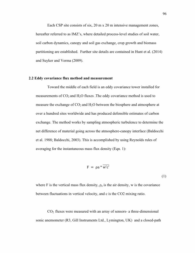
96
Each CSP site consists of six, 20 m x 20 m intensive management zones,
hereafter referred to as IMZ’s, where detailed process-level studies of soil water,
soil carbon dynamics, canopy and soil gas exchange, crop growth and biomass
partitioning are established. Further site details are contained in Hunt et al. (2014)
and Suyker and Verma (2009).
2.2 Eddy covariance flux method and measurement
Toward the middle of each field is an eddy covariance tower installed for
measurements of CO2 and H2O fluxes .The eddy covariance method is used to
measure the exchange of CO2 and H2O between the biosphere and atmosphere at
over a hundred sites worldwide and has produced defensible estimates of carbon
exchange. The method works by sampling atmospheric turbulence to determine the
net difference of material going across the atmosphere-canopy interface (Baldocchi
et al. 1988; Baldocchi, 2003). This is accomplished by using Reynolds rules of
averaging for the instantaneous mass flux density (Eqn. 1):
F = ρa * w'c'
(1)
where F is the vertical mass flux density, ρa is the air density, w is the covariance
between fluctuations in vertical velocity, and c is the CO2 mixing ratio.
CO2 fluxes were measured with an array of sensors- a three-dimensional
sonic anemometer (R3, Gill Instruments Ltd., Lymington, UK) and a closed-path
97
CO2/H2O system (LI 6262, Li-Cor Inc., Lincoln, NE) . H2O fluxes were measured
with an open-path CO2/H2O sensor (LI 7500, Li-Cor Inc., Lincoln, NE). Further
details are given in Verma et al. 2005 and Suyker et al. 2003. Eddy covariance
sensors were mounted at a height of 3.0 m above the ground until canopy height
exceeded 1.0 m. When the canopy height of maize exceeded 1.0 m, the eddy
covariance sensors were moved to a height of 6.0 m, a height they remained at until
harvest.
The CO2 storage in the layer below the eddy covariance sensors was
calculated from CO2 concentration profile measurements and added to the
measured CO2 flux to obtain the net ecosystem exchange (NEE). Estimates of
daytime ecosystem respiration were obtained from the night-NEE relationship,
which is explained further in Xu and Baldocchi, 2004. The gross primary
productivity (GPP) was obtained by taking the difference of NEE and ecosystem
respiration. All GPP values in this paper represent a daily average in units of g
C/m2/d.
2.3 Soil moisture sensors
Dynamax Theta probes were installed in the spring of 2001 at depths of 10,
25, 50, and 100 cm as part of three IMZ’s in IMS and four in RMS. Soil moisture
sensors at 10 and 25 cm were removed from all IMZ’s during planting and harvest
periods and then reinstalled in the same location.
The soil moisture probes were installed at a 45° angle from vertical to the
surface at 10 and 25 cm and were installed using the drip loop method at 50 and
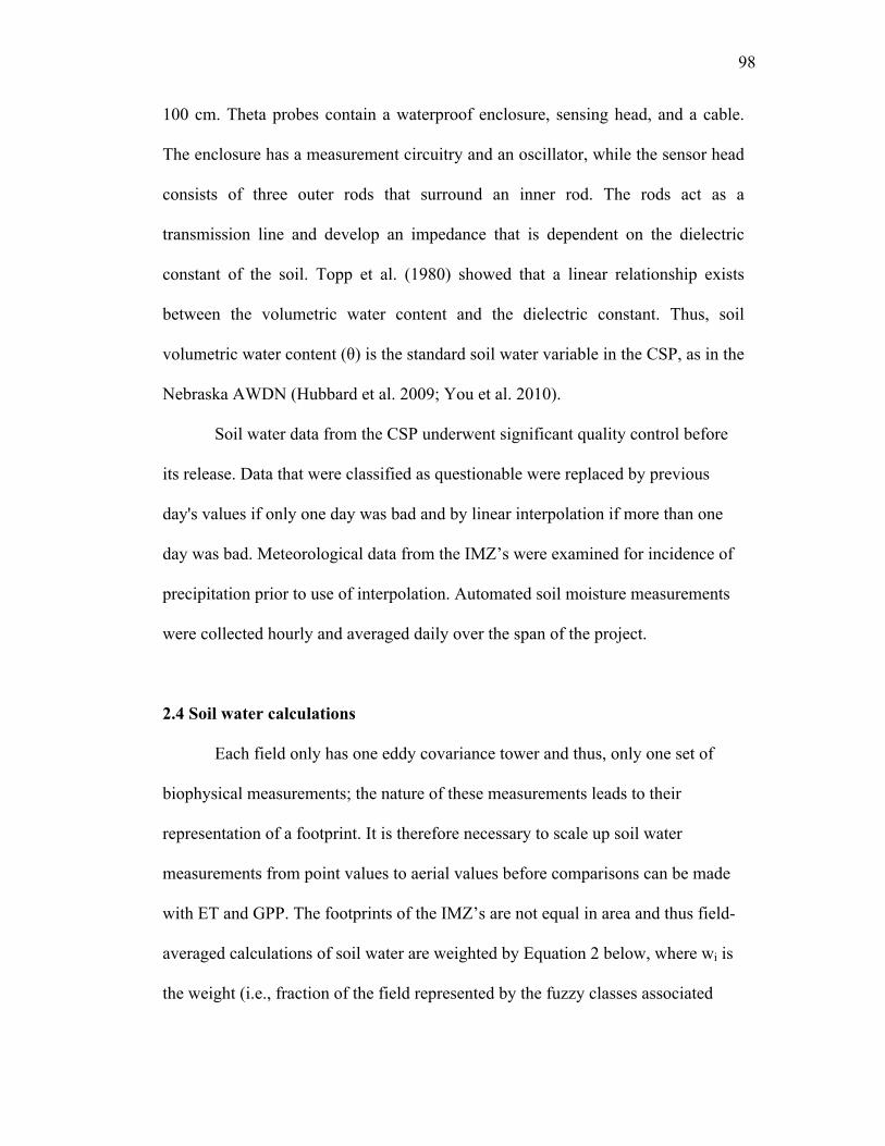
98
100 cm. Theta probes contain a waterproof enclosure, sensing head, and a cable.
The enclosure has a measurement circuitry and an oscillator, while the sensor head
consists of three outer rods that surround an inner rod. The rods act as a
transmission line and develop an impedance that is dependent on the dielectric
constant of the soil. Topp et al. (1980) showed that a linear relationship exists
between the volumetric water content and the dielectric constant. Thus, soil
volumetric water content (θ) is the standard soil water variable in the CSP, as in the
Nebraska AWDN (Hubbard et al. 2009; You et al. 2010).
Soil water data from the CSP underwent significant quality control before
its release. Data that were classified as questionable were replaced by previous
day's values if only one day was bad and by linear interpolation if more than one
day was bad. Meteorological data from the IMZ’s were examined for incidence of
precipitation prior to use of interpolation. Automated soil moisture measurements
were collected hourly and averaged daily over the span of the project.
2.4 Soil water calculations
Each field only has one eddy covariance tower and thus, only one set of
biophysical measurements; the nature of these measurements leads to their
representation of a footprint. It is therefore necessary to scale up soil water
measurements from point values to aerial values before comparisons can be made
with ET and GPP. The footprints of the IMZ’s are not equal in area and thus field-
averaged calculations of soil water are weighted by Equation 2 below, where wi is
the weight (i.e., fraction of the field represented by the fuzzy classes associated
99
with the i’th IMZ), x is the measured soil water in the i’th IMZ and i increases
from 1 to n (the total number of IMZs per field). Weights were assigned to each
IMZ based on the proportional area of the fuzzy class represented.
x = w!x!
!
!!!
(2)
Prior to the study, soil samples were collected from all IMZ’s at the three
sites and were analyzed in the laboratory for soil type and water holding capacity.
Silt clay loam is the predominant soil texture at IMZ’s in both fields. Field capacity
and wilting point values at the three sites were determined by averaging the -1/3
bar values and the -15 bar values respectively from moisture release curves
determined in the laboratory.
2.5 Potential evapotranspiration calculations
Potential evapotranspiration (ETp) was calculated for a reference alfalfa
crop using an updated version of the Penman-Monteith equation (Monteith, 1965)
outlined in Allen et al. (1998). While this method of calculating ETp
underestimates evapotranspiration of a tall maize crop, it allowed for consistent
comparisons of ETp across and between seasons and between RMS and IMS and
for direct comparisons with previously published studies. As with other variables,
ETp was calculated and summed over ten-day periods at both RMS and IMS.
100
2.6 Development stages and period definitions
The dates of specific development stages of maize were determined from
records collected during regular field observations of growth throughout the
available years of the CSP. There was usually a slight variation in a development
stage within a field, so the date listed for a particular development stage of maize is
a date when approximately 50 percent of the field was at that stage. LAI
measurements were made periodically during a season at various locations and
numbers shown in the study are field averages.
As in chapter 2, the growing season (GS) is defined as 1 May to 31
October. However, a majority of this chapter focuses on analysis from a common
90-day period (DOY 151-240) in each season. This common 90-day period (C90)
was chosen as it encompasses almost all of the critical stages of a maize plant,
from early vegetative to late in the reproductive stage. In this case, maize was
roughly at 4-leaf (V4) in every GS at DOY 151 and at the denting stage (R5) at
DOY 240.
This chapter also looks more in-depth in a window ranging from 10-days
prior to the onset of silking to 20-days subsequent. According to various reports
(Elmore 2012), maize is most vulnerable to water stress from just before silking
(R1) to the milk stage (R3). Thus, additional focus was given to this 31-day
period.

101
3.0 Results and Discussion
The following section presents an analysis of the relationship of biophysical
variables and soil water over four seasons in which maize was the common crop at
both RMS and IMS. Of the four seasons in the study period, two were drier than
the long-term average of approximately 470 mm for the GS and 280 mm for the
C90. In both of seasons, total precipitation was greatly exceeded by total
evapotranspiration (ET) and potential evapotranspiration (ETp) during the C90.
The other two seasons were wetter than the long-term average and total
precipitation exceeded ET and in 2009, precipitation equaled ETp. While there
were unifying themes across all four seasons, there are some unique similarities
and differences between the two wet (dry) seasons. The remainder of this section is
thus dedicated to that.
3.1 Dry seasons
The 2003 GS and 2005 GS were both drier than average and had final
maize yields at RMS that were much lower compared to those at IMS (Table 1).
According to chapter 2, total GS precipitation at RMS was well below the long-
term average in both seasons, with 369 mm and 329 mm in 2003 and 2005
respectively. During the C90 analyzed for this chapter, a total of 150 and 234 mm
of precipitation fell in 2003 and 2005 respectively. While both seasons had
prolonged dry spells that were detrimental to maize development, the timing of
significant water stress and the manifestations of water stress were quite different.
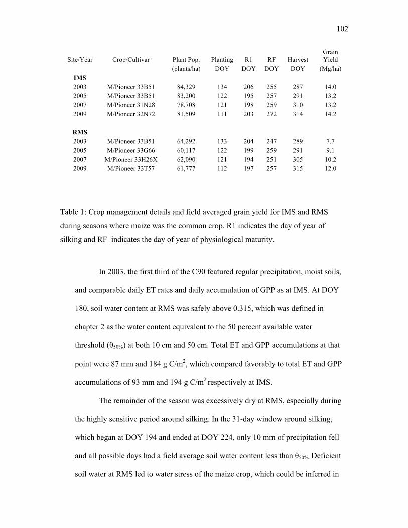
102
Site/Year Crop/Cultivar Plant Pop. Planting R1 RF Harvest Grain Yield
(plants/ha) DOY DOY DOY DOY (Mg/ha) IMS 2003 M/Pioneer 33B51 84,329 134 206 255 287 14.0 2005 M/Pioneer 33B51 83,200 122 195 257 291 13.2 2007 M/Pioneer 31N28 78,708 121 198 259 310 13.2 2009 M/Pioneer 32N72 81,509 111 203 272 314 14.2
RMS 2003 M/Pioneer 33B51 64,292 133 204 247 289 7.7 2005 M/Pioneer 33G66 60,117 122 199 259 291 9.1 2007 M/Pioneer 33H26X 62,090 121 194 251 305 10.2 2009 M/Pioneer 33T57 61,777 112 197 257 315 12.0
Table 1: Crop management details and field averaged grain yield for IMS and RMS
during seasons where maize was the common crop. R1 indicates the day of year of
silking and RF indicates the day of year of physiological maturity.
In 2003, the first third of the C90 featured regular precipitation, moist soils,
and comparable daily ET rates and daily accumulation of GPP as at IMS. At DOY
180, soil water content at RMS was safely above 0.315, which was defined in
chapter 2 as the water content equivalent to the 50 percent available water
threshold (θ50%) at both 10 cm and 50 cm. Total ET and GPP accumulations at that
point were 87 mm and 184 g C/m2, which compared favorably to total ET and GPP
accumulations of 93 mm and 194 g C/m2 respectively at IMS.
The remainder of the season was excessively dry at RMS, especially during
the highly sensitive period around silking. In the 31-day window around silking,
which began at DOY 194 and ended at DOY 224, only 10 mm of precipitation fell
and all possible days had a field average soil water content less than θ50%. Deficient
soil water at RMS led to water stress of the maize crop, which could be inferred in
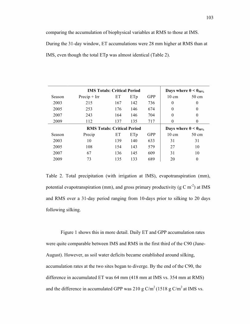
103
comparing the accumulation of biophysical variables at RMS to those at IMS.
During the 31-day window, ET accumulations were 28 mm higher at RMS than at
IMS, even though the total ETp was almost identical (Table 2).
IMS Totals: Critical Period Days where θ < θ50% Season Precip + Irr ET ETp GPP 10 cm 50 cm 2003 215 167 142 736 0 0 2005 253 176 146 674 0 0 2007 243 164 146 704 0 0 2009 112 137 135 717 0 0
RMS Totals: Critical Period Days where θ < θ50% Season Precip ET ETp GPP 10 cm 50 cm 2003 10 139 140 633 31 31 2005 108 154 143 579 27 10 2007 67 136 145 609 31 10 2009 73 135 133 689 20 0
Table 2. Total precipitation (with irrigation at IMS), evapotranspiration (mm),
potential evapotranspiration (mm), and gross primary productivity (g C m-2) at IMS
and RMS over a 31-day period ranging from 10-days prior to silking to 20 days
following silking.
Figure 1 shows this in more detail. Daily ET and GPP accumulation rates
were quite comparable between IMS and RMS in the first third of the C90 (June-
August). However, as soil water deficits became established around silking,
accumulation rates at the two sites began to diverge. By the end of the C90, the
difference in accumulated ET was 64 mm (418 mm at IMS vs. 354 mm at RMS)
and the difference in accumulated GPP was 210 g C/m2 (1518 g C/m2 at IMS vs.

104
1308 g C/m2 at RMS). Water stress was also evident in the LAI. During the 2003
flash drought, the LAI at RMS began to decline after silking, whereas the LAI at
IMS remained steady for the remainder of C90 after peaking at the end of the
vegetative stage.
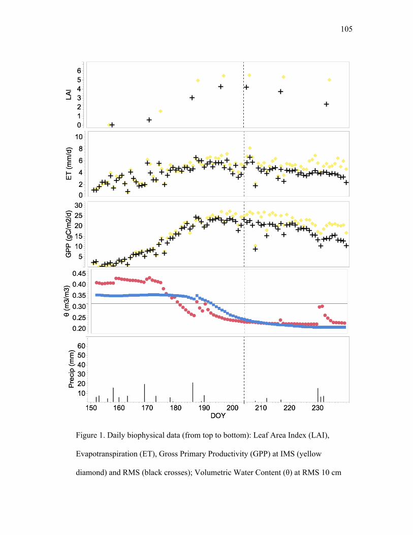
105
Figure 1. Daily biophysical data (from top to bottom): Leaf Area Index (LAI),
Evapotranspiration (ET), Gross Primary Productivity (GPP) at IMS (yellow
diamond) and RMS (black crosses); Volumetric Water Content (θ) at RMS 10 cm
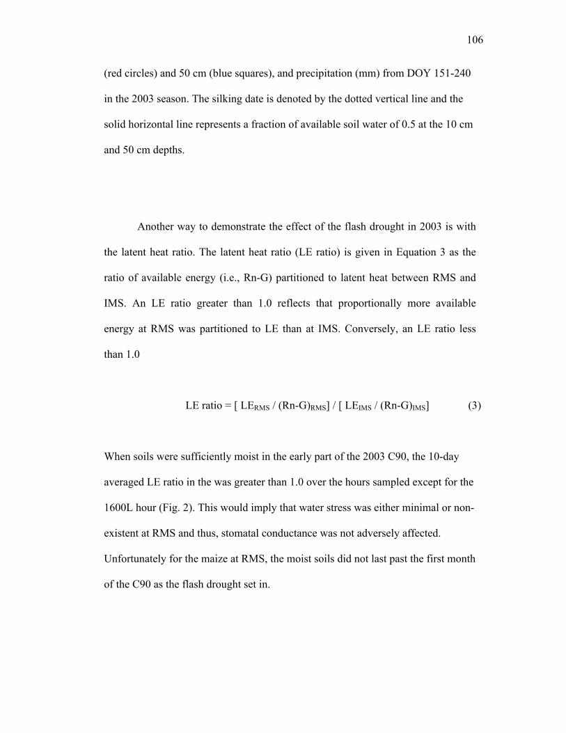
106
(red circles) and 50 cm (blue squares), and precipitation (mm) from DOY 151-240
in the 2003 season. The silking date is denoted by the dotted vertical line and the
solid horizontal line represents a fraction of available soil water of 0.5 at the 10 cm
and 50 cm depths.
Another way to demonstrate the effect of the flash drought in 2003 is with
the latent heat ratio. The latent heat ratio (LE ratio) is given in Equation 3 as the
ratio of available energy (i.e., Rn-G) partitioned to latent heat between RMS and
IMS. An LE ratio greater than 1.0 reflects that proportionally more available
energy at RMS was partitioned to LE than at IMS. Conversely, an LE ratio less
than 1.0
LE ratio = [ LERMS / (Rn-G)RMS] / [ LEIMS / (Rn-G)IMS] (3)
When soils were sufficiently moist in the early part of the 2003 C90, the 10-day
averaged LE ratio in the was greater than 1.0 over the hours sampled except for the
1600L hour (Fig. 2). This would imply that water stress was either minimal or non-
existent at RMS and thus, stomatal conductance was not adversely affected.
Unfortunately for the maize at RMS, the moist soils did not last past the first month
of the C90 as the flash drought set in.
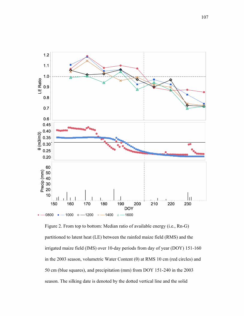
107
Figure 2. From top to bottom: Median ratio of available energy (i.e., Rn-G)
partitioned to latent heat (LE) between the rainfed maize field (RMS) and the
irrigated maize field (IMS) over 10-day periods from day of year (DOY) 151-160
in the 2003 season, volumetric Water Content (θ) at RMS 10 cm (red circles) and
50 cm (blue squares), and precipitation (mm) from DOY 151-240 in the 2003
season. The silking date is denoted by the dotted vertical line and the solid
0800 1000 1200 1400 1600
108
horizontal line represents a fraction of available soil water of 0.5 at the 10 cm and
50 cm depths.
As the season progressed and soil water became more depleted, the LE
ratios started decreasing and were less than 1.0 for all hours of the day by the time
maize entered into the reproductive stage. The biggest change occurred between
the 10-day period ending DOY 190 and the 10-day period ending DOY 210. In the
former, the LE ratio was still greater than 1.0 for all hours except 1400L. In the
latter, the LE ratio was less than 1.0 over all hours, and was safely below 1.0 in the
early part of the afternoon.
A quick peak at soil water in Figure 2 explains why this would be the case.
In the 10-days leading up to DOY 190, there was some precipitation which
temporarily brought the soil water content at 10 cm above θ50% and kept the soil
water at 50 cm safely above θ50%. However, that precipitation event was the last
one over 10 mm for over forty days and soil water declined below θ50% at both 10
cm and 50 cm shortly after DOY 190 and remained there for the duration of the
season.
The prolonged period with soil water stress had increasingly adverse effects
on stomatal conductance. By the end of the season, the 10-day average LE ratio
was significantly below 1.0 for all hours sampled and even dipped below 0.7 at the
1600L hour over the 10-day period ending DOY 230. The precipitation that fell
early in the final 10-day period of the C90 did slightly moisten the soils. However,
109
the moisture was too little and possibly too late to be of help at alleviating the
stress in the maize crop and the LE ratio did not improve.
The C90 in 2005 began in much the same way as the C90 in 2003: regular
precipitation that kept soils at RMS reasonably moist, which led to comparable
daily rates of ET and daily accumulation of GPP to those at IMS. Also, as in 2003,
a prolonged dry spell began during the vegetative stage and precipitation events for
the remainder of the season were sparse. Differences in accumulations of ET and
GPP between RMS and IMS during the C90 in 2005 were also comparable to
2003, with IMS outpacing RMS in total ET by 49 mm (64 mm in 2003) and by 185
g C/m2 (210 g C/m2 in 2003). The 2005 season was actually the driest season in the
study period and had the lowest frequency of precipitation. Thus, the two dry
seasons had much in common.
There was a key difference between the two seasons, however. As
discussed earlier and shown in Table 2, only 10 mm of precipitation fell during the
most critical 31-day window in the 2003 GS. Conversely, a total of 108 mm fell
during the 31-day window in 2005, with most of it coming with one storm on DOY
206. The main dry spell in the 2005 C90 occurred between DOY 165 and DOY
195. Precipitation in this period was almost non-existent and the dry spell led to a
decline in soil water below θ50% at both 10 cm and 50 cm by the onset of silking.
Much as in the 2003 flash drought, daily ET rates and daily accumulations of GPP
at RMS became reduced compared to those at IMS during the dry spell (Fig. 3).
The 10-day average LE ratio for the period ending DOY 190 was less than 1.0 for

110
all hours and significantly less than 1.0 during the afternoon hours as a result of the
soil water stress (Fig. 4)
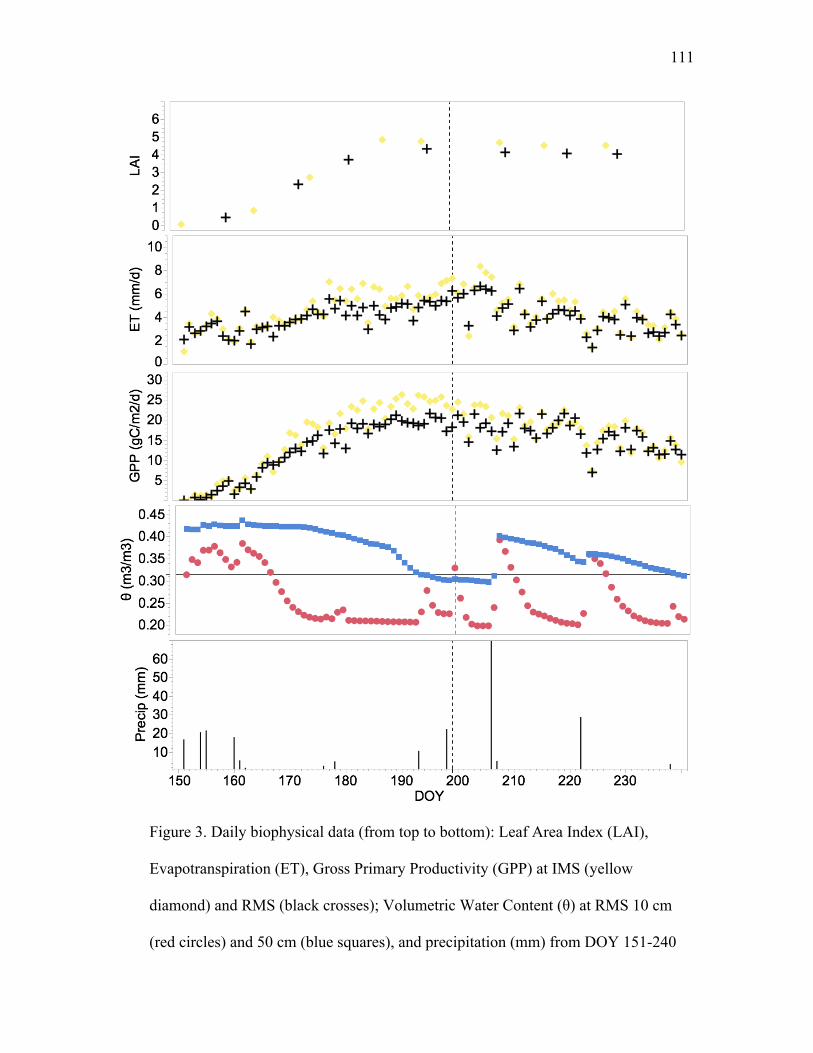
111
Figure 3. Daily biophysical data (from top to bottom): Leaf Area Index (LAI),
Evapotranspiration (ET), Gross Primary Productivity (GPP) at IMS (yellow
diamond) and RMS (black crosses); Volumetric Water Content (θ) at RMS 10 cm
(red circles) and 50 cm (blue squares), and precipitation (mm) from DOY 151-240
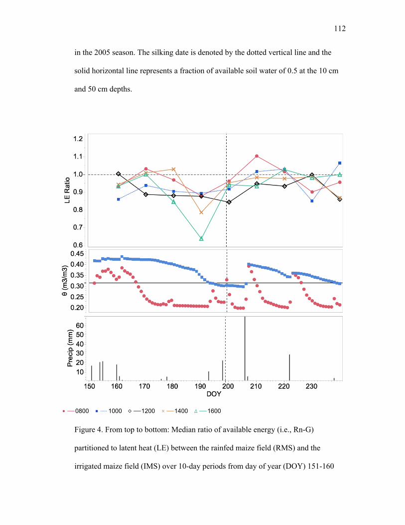
112
in the 2005 season. The silking date is denoted by the dotted vertical line and the
solid horizontal line represents a fraction of available soil water of 0.5 at the 10 cm
and 50 cm depths.
Figure 4. From top to bottom: Median ratio of available energy (i.e., Rn-G)
partitioned to latent heat (LE) between the rainfed maize field (RMS) and the
irrigated maize field (IMS) over 10-day periods from day of year (DOY) 151-160
0800 1000 1200 1400 1600
113
in the 2005 season, volumetric Water Content (θ) at RMS 10 cm (red circles) and
50 cm (blue squares), and precipitation (mm) from DOY 151-240. The silking date
is denoted by the dotted vertical line and the solid horizontal line represents a
fraction of available soil water of 0.5 at the 10 cm and 50 cm depths.
A week after the onset of silking in the 2005 GS (DOY 206), the situation
looked fairly dire for the maize crop at RMS. It was the fourth consecutive day of
maximum temperatures over 37°C, the soil water content at both 10 cm and 50 cm
were safely below θ50%, and the gap in daily ET rates and in daily GPP
accumulations were growing more significant. The LAI at RMS had not begun to
decrease markedly compared to IMS as was the case in the 2003 flash drought, but
it was likely if precipitation did not materialize soon. However, that evening a
major thunderstorm rolled through the region, bringing over 70 mm of
precipitation and much cooler weather.
This notable rainfall event was beneficial to the maize crop at RMS. Figure
3 shows that the increase in soil water from the event led to more equivocal daily
rates of ET and much closer rates of daily GPP accumulation between IMS and
RMS in the days after the storm. Perhaps the clearest example of stress alleviation
with the storm though is in the LE ratio. Figure 4 shows that the 10-day averaged
LE ratio ending on DOY 210 was greater than 1.0 in the morning hours and was
not significantly below 1.0 during the afternoon hours. Thus, the recharged soil
profile brought an almost immediate response in the form of increased stomatal
conductance at RMS compared to a few weeks earlier when it was much drier.
114
There were only two more precipitation events the remainder of the C90 in 2005.
One of them on DOY 222 was significant enough to re-moisten the soil profile,
particularly at 10 cm, which had dried out again. This kept the daily rates of ET
and accumulation of GPP somewhat close to that of IMS for most of the remainder
of the season.
As the C90 in 2005 came to a close, another dry spell was underway and as
mentioned earlier, 2005 would end up being the driest growing season in the study
period. However, the difference between 2003 and 2005 was one major storm
during the critical period. In the critical 31-day period in 2003, precipitation was
almost non-existent, and the maize crop gradually deteriorated as water stress
caused stomata to “close” at progressively earlier time in the day. In the critical 31-
day period in 2005, a significant precipitation event recharged the soil profile and
allowed stomatal conductance to recover to levels from earlier in the season.
Without that storm, it would be fair to assume that the maize yields in 2005 season
would have been worse than in 2003 as all indications from the biophysical
parameters were worse entering the critical period in 2005 than in 2003.
3.2 Wet seasons
As discussed in chapter 2, the later seasons of the study period were wetter
than the 30-year average, especially the 2007 and 2008 seasons. During the C90
analyzed for this chapter, a total of 379 and 367 mm of precipitation fell in 2007
and 2009 respectively. However, as with the dry season comparison in the previous
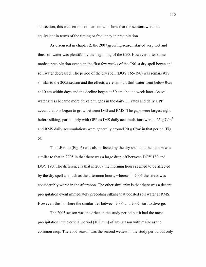
115
subsection, this wet season comparison will show that the seasons were not
equivalent in terms of the timing or frequency in precipitation.
As discussed in chapter 2, the 2007 growing season started very wet and
thus soil water was plentiful by the beginning of the C90. However, after some
modest precipitation events in the first few weeks of the C90, a dry spell began and
soil water decreased. The period of the dry spell (DOY 165-190) was remarkably
similar to the 2005 season and the effects were similar. Soil water went below θ50%
at 10 cm within days and the decline began at 50 cm about a week later. As soil
water stress became more prevalent, gaps in the daily ET rates and daily GPP
accumulations began to grow between IMS and RMS. The gaps were largest right
before silking, particularly with GPP as IMS daily accumulations were ~ 25 g C/m2
and RMS daily accumulations were generally around 20 g C/m2 in that period (Fig.
5).
The LE ratio (Fig. 6) was also affected by the dry spell and the pattern was
similar to that in 2005 in that there was a large drop off between DOY 180 and
DOY 190. The difference is that in 2007 the morning hours seemed to be affected
by the dry spell as much as the afternoon hours, whereas in 2005 the stress was
considerably worse in the afternoon. The other similarity is that there was a decent
precipitation event immediately preceding silking that boosted soil water at RMS.
However, this is where the similarities between 2005 and 2007 start to diverge.
The 2005 season was the driest in the study period but it had the most
precipitation in the crticial period (108 mm) of any season with maize as the
common crop. The 2007 season was the second wettest in the study period but only

116
67 mm of the season total came in the 31-day critical period around silking. While
this was certainly was better than the flash drought of 2003, no individual
precipitation event was enough to alleviate the stress at 10 cm. As the critical
period progressed, soil water at 50 cm also fell below θ50% and the signs of mild
water stress prevailed. Daily accumulation of GPP and daily ET rates remained less
at RMS than at IMS, though not as significant of a difference as in the 2003 flash
drought case.
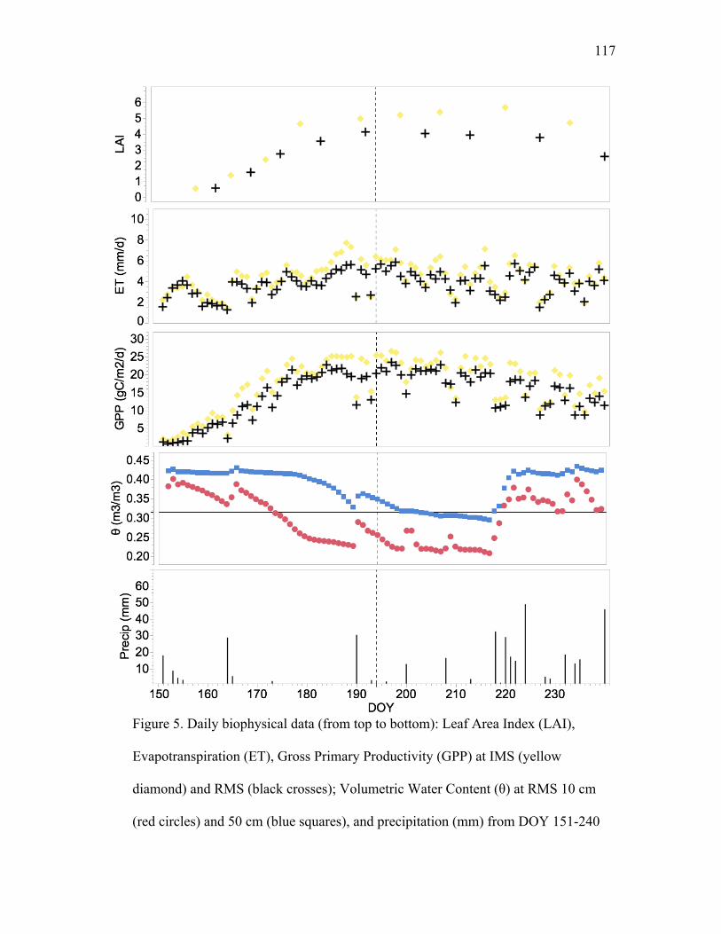
117
Figure 5. Daily biophysical data (from top to bottom): Leaf Area Index (LAI),
Evapotranspiration (ET), Gross Primary Productivity (GPP) at IMS (yellow
diamond) and RMS (black crosses); Volumetric Water Content (θ) at RMS 10 cm
(red circles) and 50 cm (blue squares), and precipitation (mm) from DOY 151-240
118
in the 2007 season. The silking date is denoted by the dotted vertical line and the
solid horizontal line represents a fraction of available soil water of 0.5 at the 10 cm
and 50 cm depths.
Figure 6. From top to bottom: Median ratio of available energy (i.e., Rn-G)
partitioned to latent heat (LE) between the rainfed maize field (RMS) and the
irrigated maize field (IMS) over 10-day periods from day of year (DOY) 151-160
0800 1000 1200 1400 1600
119
in the 2007 season, volumetric Water Content (θ) at RMS 10 cm (red circles) and
50 cm (blue squares), and precipitation (mm) from DOY 151-240. The silking date
is denoted by the dotted vertical line and the solid horizontal line represents a
fraction of available soil water of 0.5 at the 10 cm and 50 cm depths.
While the 2005 season had the major precipitation event during the critical
period, which more or less “saved” the maize crop at RMS, the 2007 season had
some modest precipitation events in July that prevented significant water stress and
therefore kept the crop going. After the 31-day critical period was over, significant
precipitation returned to the region and soils were generally very moist for the
remainder of the season. During the moist finish to the season, the 10-day averaged
LE ratios were closer to 1.0, especially in the morning. However, the gap in daily
ET rates and daily GPP accumulations did not change much over the later period
where soils at RMS were moist. A closer look at the LAI in Figure 5 shows why
this gap remained.
The LAI of maize generally increases rapidly in the first few months after
planting (i.e., early and middle vegetative stage) and reaches a maximum around
silking. Thus the maximum LAI is highly susceptible to water stress in this period.
In the 2007 season, the dry spell coincided with the period when LAI was starting
to reach its peak and thus, the max LAI at RMS was limited to a maximum of 4.1
from measurements taken on DOY 192. Conversely at IMS, where water-stress
was avoided, LAI peaked at 5.7 about three weeks after the onset of silking. This
higher LAI therefore permitted greater rates of ET and accumulations of GPP at
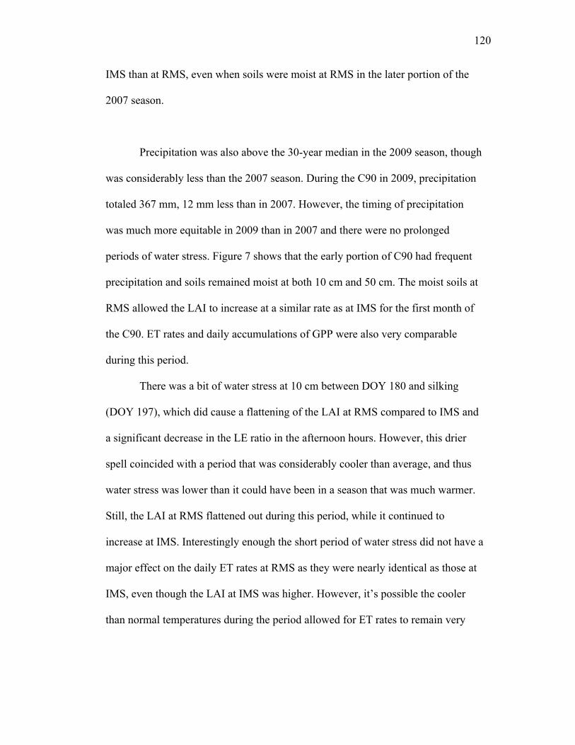
120
IMS than at RMS, even when soils were moist at RMS in the later portion of the
2007 season.
Precipitation was also above the 30-year median in the 2009 season, though
was considerably less than the 2007 season. During the C90 in 2009, precipitation
totaled 367 mm, 12 mm less than in 2007. However, the timing of precipitation
was much more equitable in 2009 than in 2007 and there were no prolonged
periods of water stress. Figure 7 shows that the early portion of C90 had frequent
precipitation and soils remained moist at both 10 cm and 50 cm. The moist soils at
RMS allowed the LAI to increase at a similar rate as at IMS for the first month of
the C90. ET rates and daily accumulations of GPP were also very comparable
during this period.
There was a bit of water stress at 10 cm between DOY 180 and silking
(DOY 197), which did cause a flattening of the LAI at RMS compared to IMS and
a significant decrease in the LE ratio in the afternoon hours. However, this drier
spell coincided with a period that was considerably cooler than average, and thus
water stress was lower than it could have been in a season that was much warmer.
Still, the LAI at RMS flattened out during this period, while it continued to
increase at IMS. Interestingly enough the short period of water stress did not have a
major effect on the daily ET rates at RMS as they were nearly identical as those at
IMS, even though the LAI at IMS was higher. However, it’s possible the cooler
than normal temperatures during the period allowed for ET rates to remain very
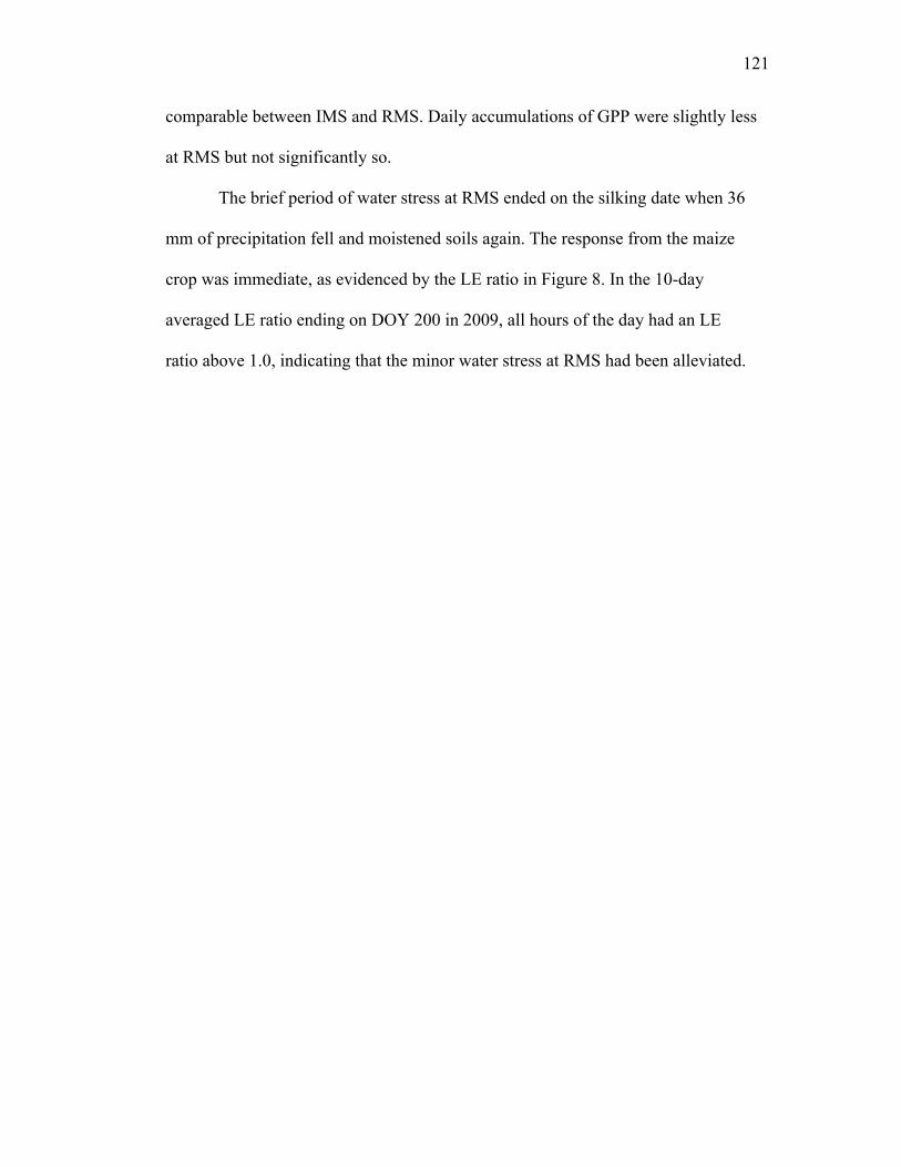
121
comparable between IMS and RMS. Daily accumulations of GPP were slightly less
at RMS but not significantly so.
The brief period of water stress at RMS ended on the silking date when 36
mm of precipitation fell and moistened soils again. The response from the maize
crop was immediate, as evidenced by the LE ratio in Figure 8. In the 10-day
averaged LE ratio ending on DOY 200 in 2009, all hours of the day had an LE
ratio above 1.0, indicating that the minor water stress at RMS had been alleviated.
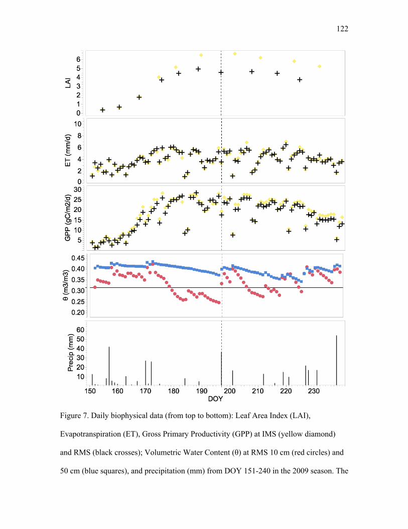
122
Figure 7. Daily biophysical data (from top to bottom): Leaf Area Index (LAI),
Evapotranspiration (ET), Gross Primary Productivity (GPP) at IMS (yellow diamond)
and RMS (black crosses); Volumetric Water Content (θ) at RMS 10 cm (red circles) and
50 cm (blue squares), and precipitation (mm) from DOY 151-240 in the 2009 season. The
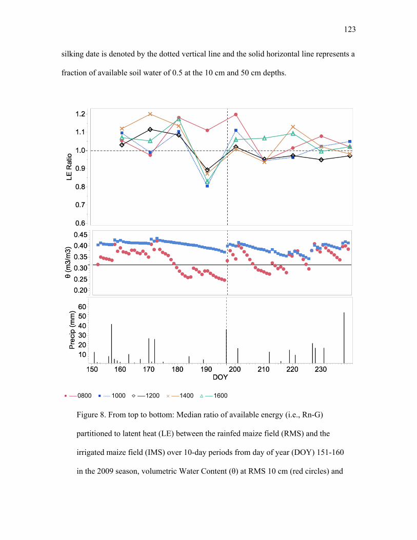
123
silking date is denoted by the dotted vertical line and the solid horizontal line represents a
fraction of available soil water of 0.5 at the 10 cm and 50 cm depths.
Figure 8. From top to bottom: Median ratio of available energy (i.e., Rn-G)
partitioned to latent heat (LE) between the rainfed maize field (RMS) and the
irrigated maize field (IMS) over 10-day periods from day of year (DOY) 151-160
in the 2009 season, volumetric Water Content (θ) at RMS 10 cm (red circles) and
0800 1000 1200 1400 1600
124
50 cm (blue squares), and precipitation (mm) from DOY 151-240. The silking date
is denoted by the dotted vertical line and the solid horizontal line represents a
fraction of available soil water of 0.5 at the 10 cm and 50 cm depths.
The remainder of the 2009 season featured several modest precipitation
events and continued cooler than average temperatures, and there were no
prolonged periods of soil water stress. Thus, daily ET rates at RMS remained
almost identical to those of IMS throughout the remainder of the C90. Daily
accumulations of GPP were a bit less at RMS than at IMS, which as in 2007, could
be explained by the lower LAI at RMS. Still, the accumulated GPP at RMS during
the C90 was only 112 g C/m2 less than at IMS and at 1543 g C/m2, it was by far the
highest accumulation of GPP of any season when maize was the common crop at
RMS and IMS.
4.0 Summary and Conclusions
Dry periods were common in the study period. Every season, except the
2009 GS, had at least one 10-day period with less than 10 mm of precipitation at
RMS. However, as shown in chapter 2, timing of precipitation was very important.
For example, the 2005 GS actually had more 10-day periods (5 total) with less than
10 mm of precipitation than the 2003 flash drought season (3 total). However, the
overall maize yields were higher in 2005 (see Table 1) due to the occurrence of a
couple of significant precipitation events in what was otherwise a very dry season.
Likewise, maize yields were much higher in 2009 than in 2007, even though the
125
2007 GS had more precipitation. The difference again was timing. In the 2007 GS,
a significant portion of the precipitation fell in mid-to-late August, but was
somewhat dry during the critical period from just before to a few weeks after
silking. Conversely, in the 2009 GS, regular precipitation occurrences prevented
prolonged water stress, especially during the aforementioned critical period.
As expected, total ET and GPP were higher, sometimes significantly so, at
IMS than at RMS over this period. ETp was very consistent within a season
between RMS and IMS and with the exception of the abnormally cool 2009
season, was fairly consistent between seasons. During the dry spells, soil water
stress often caused noticeable reductions in the LE ratio, as the closing of stomata
in response to a lack of soil water led to less of the available energy being
portioned to latent heat at RMS compared to IMS. During the inception of water
stress, this effect was strongest in the afternoon hours. As the water stress
persisted, the effect was realized earlier in the day.
Maize at RMS did appear to have some resilience, and while we can only
imply levels of stomatal conductance from the figures shown, it seems clear from
the ET and GPP data and the LE ratios that a significant recharge of soil water after
incipient water stress can lead to rejuvenation of the maize crop, even if the
potential yield has been cut. The biggest difference between 2005 and 2003 was a
major storm occurred at a point of stress in 2005 and not in 2003. If a storm of
equal magnitude had occurred during the critical period in 2003, it is very likely
that we would only be discussing 2003 as a bit drier than normal season with a
126
modest reduction in overall yield potential and not as an idealized flash drought
scenario.
5.0 Acknowledgements:
The research presented here was supported by the Office of Science (BER), U.S.
Department of Energy Grant (No. DE-FG02-03ER63639 and the University of
Nebraska-Lincoln Program of Excellence. Special thanks to Todd Schimelfenig for
providing technical expertise and data.
127
6.0 References
Baldocchi, D.D., Hicks, B.B., Meyers, T.P., 1988. Measuring biosphere-
atmosphere exchanges of biologically related gases with micrometeorological
methods. Ecology 69 (5), 1331-1340.
Baldocchi, D.D., 2003. Assessing the eddy covariance technique for evaluating
carbon dioxide exchange rates of ecosystems: past, present, and future. Global
Change Biol. 9 (4), 479-492.
Elmore, R. 2012. Stress, anthesis-silk interval and corn yield potential. Integrated
Crop Management News. Iowa State University Extension and Outreach.
Hubbard, K.G., You, J., Sridhar, V., Hunt, E., Korner, S., Roebke, G., 2009. Near-
surface soil water monitoring for water resources management on a wide-area basis
in the Great Plains. Great Plains Res., 19, 45-54.
Hunt, E.D., Svoboda, M., Wardlow, B., Hubbard, K., Hayes, M., Arkebauer, T.
2014. Monitoring the effects of rapid onset of drought on non-irrigated maize with
agronomic data and climate-based drought indices. Agric. For. Meteorol. 191, 1-
11.
Suyker, A.E., Verma, S.B., Burba, C.G. 2003. Interannual variability in net CO2
exchange of a native tallgrass prairie. Global Change Biol. 9, 1-11.
128
Suyker, A.E., Verma, S.B., Burba, G.G., Arkebauer, T.J., Walters, D.T., Hubbard,
K.G., 2004. Growing season carbon dioxide exchange in irrigated and rainfed
maize, Agric. For. Meteorol. 124, 1-13.
Suyker, A. E., Verma, S.B., 2008. Interannual water vapor and energy exchange in
an irrigated maize-based agroecosystem. Agricul. For. Meteorol. 148, 417-427.
Suyker, A. E., Verma, S.B., 2009. Evapotranspiration of irrigated and rainfed
maize-soybean cropping systems. Agricul. For. Meteorol. 149, 443-452.
Suyker, A.E., Verma, S.B., 2012. Gross primary production and ecosystem
respiration of irrigated and rainfed maize-soybean cropping system over 8 years.
Agric. For. Meteorol. 165, 12-24.
Topp, G.C., Davis, J.L. Annan, A.P., 1980. Elecctromagentic determination of soil
water content: measurement in coaxial transmission lines. Water Resour. Res. 16,
574-582.
Verma, S.B., Dobermann, A., Cassman, K.G., Walters, D.T., Knops, J.M.,
Arkebauer, T.J., Suyker, A.E., Burba, G.G., Amos, B., Yang, H., Ginting, D.,
Hubbard, K.G., Gitelson, A.A., Walter-Shea, E.A., 2005. Annual carbon dioxide
129
exchange in irrigated and rainfed maize-based agroecosystems. Agricul. For.
Meteorol. 131, 77-96.
You, J., K.G. Hubbard, Mahmood, R., Srihar, V., Todey, D., 2010. Quality control
of soil water data in Applied Climate Information System - case study in Nebraska.
J. Hydrol. Eng. 15, 200-209.
130
CHAPTER 4: MONITORING THE EFFECTS OF RAPID ONSET OF DROUGHT ON NON-IRRIGATED MAIZE WITH AGRONOMIC DATA AND CLIMATE-BASED DROUGHT INDICES
Abstract
The 2003 growing season at Mead, NE began with moist and relatively cool
conditions that persisted through most of June. During this moist phase of the
season, soil water and parameters such as evapotranspiration (ET) and gross
primary productivity (GPP) were nearly identical between a rainfed maize site
(RMS) and an irrigated maize site (IMS). A drying phase began in late June,
causing decline in soil water at RMS and the necessity of irrigation treatments at
IMS. The drying phase turned into a “stressed” phase by early August, as only 10
mm of precipitation fell in a forty day period between mid-July and late August.
Conditions at RMS began to deteriorate even more rapidly after maize entered the
critical reproductive stage, as the depletion of soil water led to (implied) reductions
in stomatal conductance, which led to significant reductions in ET and GPP,
compared to the well-watered IMS. Two drought indices, the Standardized
Precipitation Index (SPI) and the Standardized Precipitation Evapotranspiration
Index (SPEI), were utilized to show the effectiveness of short-term indices at
detecting flash drought versus field measurements. Results showed that both the 1-
month SPI and the 1-month SPEI were quite sensitive to the onset of the flash
drought and closely followed the decline in soil water and other biophysical
parameters at RMS relative to IMS. Significant precipitation returned and led to
some recharge prior to harvest but was far too late to be of any help to the maize at
RMS, as the yield difference of 6.3 Mg/ha between RMS and IMS revealed the
131
detrimental effects of a rapid onset of drought during the critical reproductive stage
of maize.
1.0 Introduction
Soil water is an integral part of the hydrologic cycle and a critical parameter
for plant growth and development. Dale and Shaw (1965) reported that soil water
is one of the most critical factors for crop development and yield. Soil water stress
at the silking stage of maize (Zea mays L.) can reduce grain yield by 50%
(Denmead and Shaw, 1960) and an omission of a single irrigation treatment at a
critical stage could reduce maize yields by up to 40% (Cakir, 2004). Meyer et al.
(1993) reported that maize was most sensitive to water stress in the silking-blister
dough stage and Calvino et al. (2003) showed a curvilinear response of maize yield
to available water in the three weeks preceding and following silking. Earl and
Davis (2003) reported maize yield reductions up to 85% during severe water stress
that occurred after the sixth leaf stage in Georgia. Thus, it is well established that a
lack of soil water causes stress and yield reduction in maize. But soil water is not a
commonly measured variable at NOAA Cooperative (COOP) weather stations and
there are but a handful of networks around the United States where soil water is a
standard, quality controlled observation (Hollinger and Isard, 1994; Illston et al.
2008; Hubbard et al. 2009).
Drought is a natural, recurring phenomena that occurs everywhere at
various points in time and is occurring somewhere on Earth at any given point of
time. Drought is a complex topic with ecosystem impacts that vary with its
132
intensity and duration and socio-economic impacts that often magnify problems for
the most vulnerable members of society. Perhaps it is fitting that drought does not
have a universal definition and is often considered in the context of four broad
categories defined by Wilhite and Glantz (1985): meteorological, agricultural,
hydrological, and socioeconomic.
Short-term drought, sometimes referred to as flash drought, is a rapid onset
of drought often accompanied by high temperatures and winds that lead to rapid
soil moisture depletion during a critical time in the growing season (Svoboda et al.
2002). Flash droughts can occur within a longer period of normal or above normal
precipitation and bring devastating agricultural impacts. For example, although
precipitation was above normal in most of Oklahoma during 1998, an intense,
short-term drought during the summer decimated the state’s cotton and peanut crop
(Basara et al. 1998; Illston and Basara, 2003). Illston et al. (2004) described four
phases of soil moisture in a flash drought case in Oklahoma: a moist plateau in the
spring, transitional drying early in the summer, enhanced drying mid-summer into
early autumn, and recharge during the cooler months of late autumn and winter.
The 2003 growing season at Mead, NE closely matches the description of
flash drought given in Svoboda et al. (2002). It began with moist and cool
conditions that persisted through much of June. However, a prolonged period of
minimal precipitation with periodic spells of heat led to a rapid decline in soil
water at a rainfed maize site compared to a nearby irrigated site, which led to
significant reductions in biophysical parameters such as evapotranspiration (ET)
and gross primary productivity (GPP). The time series of soil moisture from the

133
growing season at the rainfed maize site closely follows the four phases introduced
in Illston et al. (2004). Thus, the primary goal of this paper is to show the
relationship between soil water and agroecological parameters (ET and GPP)
during four phases of the growing season. A secondary goal of this paper is to
show the utility of using short-term and longer-term drought indices for monitoring
a flash drought that occurred during the critical reproductive stage of maize at a
rainfed site. The remainder of this section describes a short history of drought
indices, with a particular focus on the two normalized drought indices used in this
study- the Standardized Precipitation Index (SPI) and the Standardized
Precipitation Evaporatranspiration Index (SPEI).
Palmer (1965) developed the Palmer Drought Severity Index (PDSI) with
an objective of “developing a general methodology for evaluating drought in terms
of an index that permits time and space comparisons of drought severity." The
PDSI is calculated from a simple water balance model that uses factors such as
precipitation, temperature and latitude for the calculation of potential
evapotranspiration (Thornthwaite, 1948), recharge, runoff, and soil moisture loss to
determine whether recent precipitation was sufficient to maintain a normal water
balance. The PDSI is divided into 11 categories ranging from extreme drought to
extreme wet spell (Heim, 2002).
McKee et al. (1993) developed the Standardized Precipitation Index (SPI)
in response to demand from Colorado decision makers for an index that expressed
current conditions in terms of water supply, deficit, and probability. The SPI has
the advantage of being spatially invariant and an indicator of drought on multiple
134
time scales (Guttman, 1999), though caution has been advised when comparing the
SPI between sites with very different periods of record and at short time scales
during distinct dry seasons (Wu et al. 2005).
The SPI has been widely used for operational and research purposes. Hayes
et al. (1999) showed that the SPI detected drought conditions a full month ahead of
the PDSI during the U.S. southern Plains drought of 1996. Livida and
Assemakopoulos (2007) used the SPI to show that mild and moderate drought were
more common on the three- and six- month time scale across northern Greece
while severe drought was more frequent across southern Greece. Brown et al.
(2008) integrated the SPI with satellite derived vegetation metrics and biophysical
data to produce 1-km maps of the Vegetation Drought Response Index (VegDRI).
McRoberts and Nielsen-Gammon (2012) used daily precipitation from the
Advanced Hydrologic Prediction Service multisensor precipitation estimates
(MPE) and COOP station data to obtain a high resolution SPI to be used as
guidance for the U.S. Drought Monitor (Svoboda et al. 2002). Thus, it was
recommended by the World Meteorological Organization to be the primary
drought index for national meteorological and hydrological agencies in monitoring
meteorological drought across the globe (Hayes et al. 2011).
One criticism of a precipitation-only index like the SPI is that it does not
account for temperature effects on drought. For example, Hu and Wilson (2000)
showed that the temperature and precipitation dependent PDSI was affected by
both large anomalies of temperature and precipitation in the central United States.
Vicente-Serrano et al. (2010) addressed this issue with the development of the
135
SPEI. The SPEI is based on the monthly (or weekly) difference between
precipitation and potential evapotranspiration (ETp), using the ETp method from
Thornthwaite (1948). The Thornthwaite method of ETp was chosen over more
robust methods, such as the Penman-Monteith (Monteith, 1964), due to the
simplicity of its calculation and its reasonable performance when calculating a
drought index, such as the PDSI (Mavromatis, 2007).
The development of drought indices allows for useful comparisons of
conditions between locations and over long periods of time. However, caution
should still be applied when applying an index to long time-series of climate data.
Inhomogeneities in data from station relocations, instrumentation changes, and
growth of vegetation and urban boundaries do exist and analyses can be erroneous
if these items are not accounted for (Peterson et al. 1998). Nevertheless, climate-
based drought indices are useful at identifying the severity and duration of drought
and continued research will only make existing indices more accurate and robust.
2.0 Materials and methods
2.1. Study site
The CSP is located at the University of Nebraska-Lincoln (UNL)
Agricultural Research and Development Center near the town of Mead, NE. The
CSP commenced in the spring of 2001 and consists of three sites. The first
agroecosystem is an irrigated, continuous maize (ICM) site centered at 41˚09’54.2”
N, 96˚ 28’35.9” W with an irrigated area of 48.7 ha. The second agroecosystem is
136
an irrigated, rotated maize-soybean (IMS) site centered at 41˚09’53.5” N, 96˚
28’12.3” W with an irrigated area of 52.4 ha. Both ICM and IMS were irrigated
rotations of maize and soybeans under no-till in the ten years prior to the
initialization of the CSP. The third agroecosystem is a rainfed, rotated maize-
soybean (RMS) site centered at 41˚10’46.8” N, 96˚ 26’22.7” W with an area of
65.4 ha. Prior to the CSP, RMS had 2-4 ha plots of maize, soybeans, wheat, and
oats with tillage (Verma et al. 2005). ICM was not considered in this analysis as its
management practice (i.e., continuous maize) made it less comparable to RMS than
IMS.
Each CSP site consists of six, 20 m x 20 m intensive management zones,
hereafter referred to as IMZ’s, where detailed process-level studies of soil water,
soil carbon dynamics, canopy and soil gas exchange, crop growth and biomass
partitioning are established. Prior to the onset of the CSP in 2001, all three sites
were uniformly tilled by disking the top 10 cm to incorporate Phosphorous (P) and
Potassium (K) fertilizers and to homogenize the soil layer (Suyker and Verma,
2009). Nitrogen (N) fertilizer applications were applied to IMS and RMS prior to
planting in 2003; subsequent N applications were applied in June at IMS through
the center-pivot system in a process known as fertigation.
The IMZ locations were selected using k-means clustering applied to six
layers of 4 m x 4 m cells based broadly on soil type, topography, and crop
production potential within each site. Fine-scale spatial information used for each
site included a digital soil map, a digital elevation model, a Veris map of soil
electrical conductivity (0-30 cm), near infrared reflectance of bare soil from the
137
IKONOS satellite (4 km resolution), and a map of soil organic matter (0-20 cm).
Interpolation onto a 4 x 4 m grid was done by kriging.
2.2 Eddy covariance flux method and measurement
Toward the middle of each field is an eddy covariance tower installed for
measurements of CO2 and H2O fluxes. The eddy covariance method is used to
measure the exchange of CO2 and H2O between the biosphere and atmosphere at
over a hundred sites worldwide and has produced defensible estimates of carbon
exchange. The method works by sampling atmospheric turbulence to determine the
net difference of material going across the atmosphere-canopy interface (Baldocchi
et al. 1988; Baldocchi, 2003).
CO2 fluxes were measured with an array of sensors- a three-dimensional
sonic anemometer (R3, Gill Instruments Ltd., Lymington, UK) and a closed-path
CO2/H2O system (LI 6262, Li-Cor Inc., Lincoln, NE) . H2O fluxes were measured
with an open-path CO2/H2O sensor (LI 7500, Li-Cor Inc., Lincoln, NE). Further
details are given in Verma et al. 2005 and Suyker et al. 2003. Eddy covariance
sensors were mounted at a height of 3.0 m above the ground until canopy height
exceeded 1.0 m. When canopy height exceeded 1.0 m, the eddy covariance sensors
were moved to a height of 6.0 m, a height they remained at until harvest.
The CO2 storage in the layer below the eddy covariance sensors was
calculated from CO2 concentration profile measurements and added to the
measured CO2 flux to obtain the net ecosystem exchange (NEE). Estimates of
daytime ecosystem respiration were obtained from the night-NEE relationship,
138
which is explained further in Xu and Baldocchi, 2004. The gross primary
productivity (GPP) was obtained by taking the difference of NEE and ecosystem
respiration. All GPP values in this paper represent a daily average in units of g
C/m2/d.
2.3 Soil moisture sensors
Dynamax Theta probes were installed in the spring of 2001 at depths of 10,
25, 50, and 100 cm as part of three IMZ’s in IMS and four in RMS. Soil moisture
sensors at 10 and 25 cm were removed from all IMZ’s during planting and harvest
periods and then reinstalled in the same location.
The soil moisture probes were installed at a 45° angle from vertical to the
surface at 10 and 25 cm and were installed using the drip loop method at 50 and
100 cm. Theta probes contain a waterproof enclosure, sensing head, and a cable.
The enclosure has a measurement circuitry and an oscillator, while the sensor head
consists of three outer rods that surround an inner rod. The rods act as a
transmission line and develop an impedance that is dependent on the dielectric
constant of the soil. Topp et al. (1980) showed that a linear relationship exists
between the volumetric water content and the dielectric constant. Thus, soil
volumetric water content (θ) is the standard soil water variable in the CSP, as in the
Nebraska AWDN (Hubbard et al. 2009; You et al. 2010).
Soil water data from the CSP underwent significant quality control before
its release. Data that were classified as questionable were replaced by previous
day's values if only one day was bad and by linear interpolation if more than one
139
day was bad. Meteorological data from the IMZ’s were examined for incidence of
precipitation prior to use of interpolation. Automated soil moisture measurements
were collected hourly and averaged daily over the span of the project.
2.4 Soil water calculations
Each field only has one eddy covariance tower and thus, only one set of
measurements of ET, GPP, and related parameters; the nature of these
measurements leads to their representation of a footprint. It is therefore necessary
to scale up soil water measurements from point values to aerial values before
comparisons can be made with ET. The footprints of the IMZ’s are not equal in
area and thus field-averaged calculations of soil water are weighted by Equation 1
below, where wi is the weight (i.e., fraction of the field represented by the fuzzy
classes associated with the i’th IMZ), x is the measured soil water in the i’th IMZ
and i increases from 1 to n (the total number of IMZs per field). Weights were
assigned to each IMZ based on the proportional area of the fuzzy class represented.
x = w!x!
!
!!!
(1)
Prior to the study, soil samples were collected from all IMZ’s at the three
sites and were analyzed in the laboratory for soil type and water holding capacity.
Silt clay loam is the predominant soil texture at IMZ’s in both fields. Field capacity
and wilting point values at the three sites were determined by averaging the -1/3
bar values and the -15 bar values respectively from moisture release curves

140
determined in the laboratory. A fraction of available soil water (FAW) was
calculated via Equation 2 for a direct comparison of available soil water between
IMS and RMS and is used hereafter for soil water comparisons in this paper. The
FAW is weighted by IMZ (refer to Eqn. 1) and weighted by root density of maize
(Tufekcioglu et al. 1999) to obtain a field average FAW. Values of FAW range from
0 at the wilting point (θWP) to 1 at field capacity (θFC), though values over 1 are
possible for short periods if θ is between saturation and field capacity.
F!" = (θ-‐θ!") (θ!"-‐θ!")
(2)
2.5 Development stages
The dates of specific development stages of maize were determined from
records collected during regular field observations of growth throughout the
available years of the CSP. There was usually a slight variation in a development
stage within a field, so the date listed for a particular development stage of maize is
a date when approximately 50 percent of the field was at that stage.
2.6 Calculation of SPI and SPEI
Since precipitation is generally not normally distributed, it is necessary to
apply a transformation to the probability of observed precipitation for a set time
period (i.e., 1-month, 3-months, etc…) to obtain a normalized index. A three-
parameter Pearson-Type III distribution was found to be the best universal model
141
for calculation of the SPI (Guttman, 1999), although a two-parameter gamma
distribution was also shown to yield good results. The cumulative probability
distribution is then transformed into a standard normal distribution using an
approximate conversion from Abramowitz and Stegun, 1965. The values for the
SPI are analogous to the number of standard deviations above or below the mean
and generally range from -3.0 to 3.0. For a more thorough description of the SPI
calculation, refer to Lloyd-Hughes and Saunders, 2002.
The SPEI (Vicente-Serrano et al. 2010) is based on the difference (D)
between precipitation and ETp for a period of time, i, as given in Eqn. 3:
D! = P-‐ET!
(3)
where P is precipitation (mm) and ETp is the Thornthwaite method for potential
ET. Mavromatis, 2007 showed that other methods of ETp are not necessarily
superior when used in calculation of a drought index and the Thornthwaite method
requires fewer inputs than other methods, such as Penman-Monteith. Thus, the
Thornthwaite method was used for ETp in the calculation of the SPEI in this study.
The process for calculation of the SPEI is slightly more complex than that
of the SPI in part because the distribution of Di is very likely to contain negative
values. Thus, a three-parameter distribution is required for the SPEI, whereas a
two-parameter gamma distribution can suffice for the SPI. L-moment ratio
(Hosking, 1990) diagrams are used for Di as it allows for the comparison of the
empirical frequency of the series with different theoretical distributions. The L-
moment ratios are adjusted by a three-parameter log-logistic distribution to obtain a
142
cumulative probability distribution. From there, the calculation of the SPEI follows
the steps of the SPI calculation. For further SPEI calculation details, refer to the
step-by-step procedure outlined in Vicente-Serrano et al. (2010).
A 1-month and 9-month SPI and SPEI are used for comparison in this
study. Both indices were calculated at ten- day intervals beginning with 30 May
(DOY 150) and ending with 7 September (DOY 250). The Applied Climate
Information System (Hubbard et al. 2004) was used to collect data used for
analysis in this paper. Data for the SPI and SPEI come from nearby Lincoln, NE.
Data used in the study come from multiple locations in Lincoln, though the
majority of the period of record comes from the Lincoln Municipal Airport
Automated Surface Observing System (ASOS) station (KNLK), which is 40 km to
the southwest. Distance between KLNK and the CSP site(s) is sufficient to explain
90 percent of variation in maximum temperature and just outside the distance to
explain 90 percent of variation in precipitation and minimum temperature
(Hubbard, 1994).
There are potential flaws with this method and thus do not expect the
indices to match conditions at CSP exactly. However, the long period of record
from Lincoln captures severe historical droughts (i.e., 1930’s and 1950’s), which
stations closest to Mead do not. Therefore, the 2003 drought is put in a more
representative “historical” context when using data from Lincoln, even if the
distance from Lincoln to the CSP sites is too far to match the maximum possible
variation in meteorological data. Thus, we believe the sites are close enough such
143
that normalized indices calculated from Lincoln are sufficient for approximating
the same indices over the CSP.
3.0 Results and Discussion
3.1 Field Management and weather conditions
Table 1 shows details about crop management, cultivars, final grain yield,
and dates of planting, harvest, reproductive stage entry, and beginning of
physiological maturity at IMS and RMS in years where maize was the common
crop. The planting density at RMS under maize was about 75 percent of IMS, with
an average of 62,069 plants/ha over the four years compared to an average planting
density for 81,937 plants/ha for IMS. In 2003, planting densities were 84,329 and
64,292 plants/ha at IMS and RMS respectively. Maize was planted on 13-14 May
at both sites in 2003.
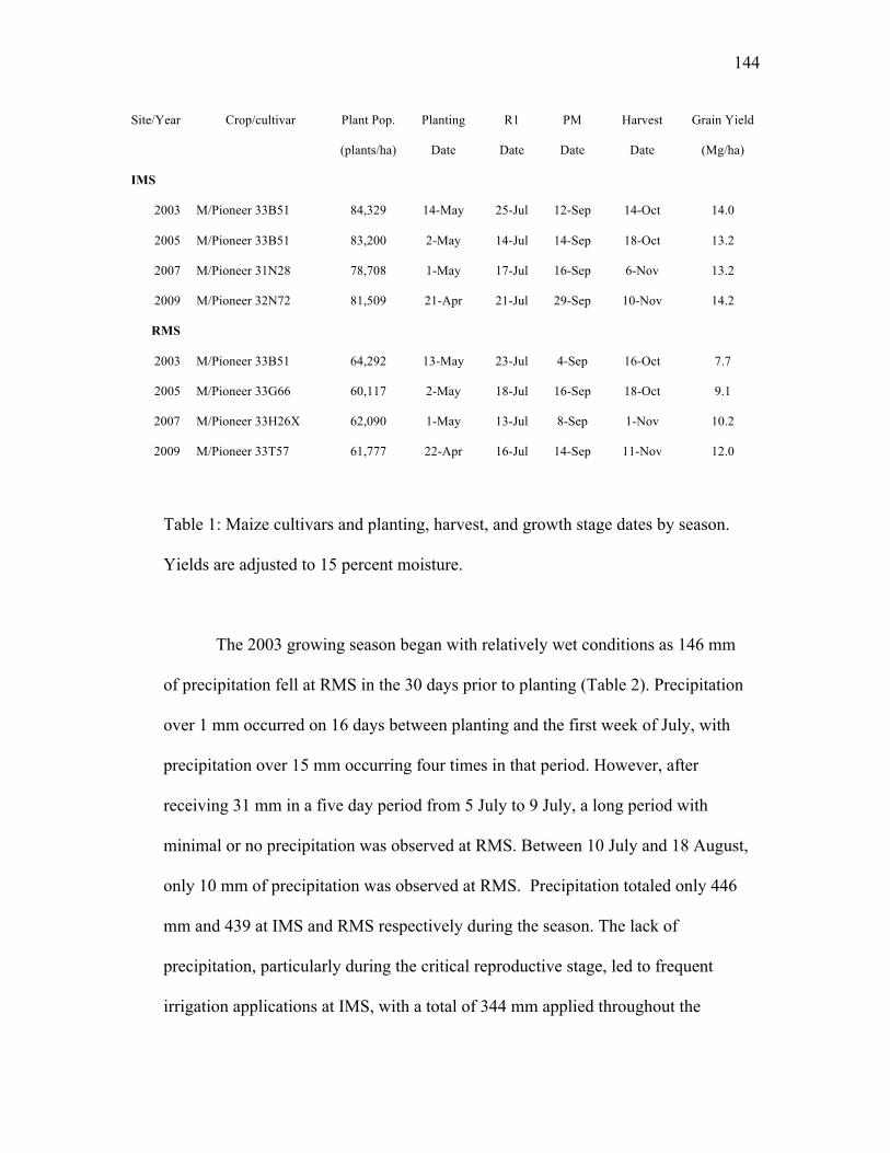
144
Table 1: Maize cultivars and planting, harvest, and growth stage dates by season.
Yields are adjusted to 15 percent moisture.
The 2003 growing season began with relatively wet conditions as 146 mm
of precipitation fell at RMS in the 30 days prior to planting (Table 2). Precipitation
over 1 mm occurred on 16 days between planting and the first week of July, with
precipitation over 15 mm occurring four times in that period. However, after
receiving 31 mm in a five day period from 5 July to 9 July, a long period with
minimal or no precipitation was observed at RMS. Between 10 July and 18 August,
only 10 mm of precipitation was observed at RMS. Precipitation totaled only 446
mm and 439 at IMS and RMS respectively during the season. The lack of
precipitation, particularly during the critical reproductive stage, led to frequent
irrigation applications at IMS, with a total of 344 mm applied throughout the
Site/Year Crop/cultivar Plant Pop. Planting R1 PM Harvest Grain Yield
(plants/ha) Date Date Date Date (Mg/ha)
IMS
2003 M/Pioneer 33B51 84,329 14-May 25-Jul 12-Sep 14-Oct 14.0
2005 M/Pioneer 33B51 83,200 2-May 14-Jul 14-Sep 18-Oct 13.2
2007 M/Pioneer 31N28 78,708 1-May 17-Jul 16-Sep 6-Nov 13.2
2009 M/Pioneer 32N72 81,509 21-Apr 21-Jul 29-Sep 10-Nov 14.2
RMS
2003 M/Pioneer 33B51 64,292 13-May 23-Jul 4-Sep 16-Oct 7.7
2005 M/Pioneer 33G66 60,117 2-May 18-Jul 16-Sep 18-Oct 9.1
2007 M/Pioneer 33H26X 62,090 1-May 13-Jul 8-Sep 1-Nov 10.2
2009 M/Pioneer 33T57 61,777 22-Apr 16-Jul 14-Sep 11-Nov 12.0
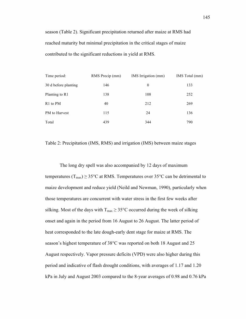
145
season (Table 2). Significant precipitation returned after maize at RMS had
reached maturity but minimal precipitation in the critical stages of maize
contributed to the significant reductions in yield at RMS.
Time period: RMS Precip (mm) IMS Irrigation (mm) IMS Total (mm)
30 d before planting 146 0 133
Planting to R1 138 108 252
R1 to PM 40 212 269
PM to Harvest 115 24 136
Total 439 344 790
Table 2: Precipitation (IMS, RMS) and irrigation (IMS) between maize stages
The long dry spell was also accompanied by 12 days of maximum
temperatures (Tmax) ≥ 35°C at RMS. Temperatures over 35°C can be detrimental to
maize development and reduce yield (Neild and Newman, 1990), particularly when
those temperatures are concurrent with water stress in the first few weeks after
silking. Most of the days with Tmax ≥ 35°C occurred during the week of silking
onset and again in the period from 16 August to 26 August. The latter period of
heat corresponded to the late dough-early dent stage for maize at RMS. The
season’s highest temperature of 38°C was reported on both 18 August and 25
August respectively. Vapor pressure deficits (VPD) were also higher during this
period and indicative of flash drought conditions, with averages of 1.17 and 1.20
kPa in July and August 2003 compared to the 8-year averages of 0.98 and 0.76 kPa
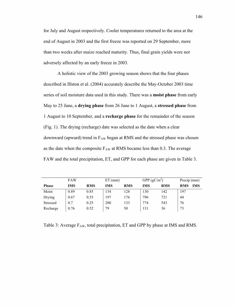
146
for July and August respectively. Cooler temperatures returned to the area at the
end of August in 2003 and the first freeze was reported on 29 September, more
than two weeks after maize reached maturity. Thus, final grain yields were not
adversely affected by an early freeze in 2003.
A holistic view of the 2003 growing season shows that the four phases
described in Illston et al. (2004) accurately describe the May-October 2003 time
series of soil moisture data used in this study. There was a moist phase from early
May to 25 June, a drying phase from 26 June to 1 August, a stressed phase from
1 August to 10 September, and a recharge phase for the remainder of the season
(Fig. 1). The drying (recharge) date was selected as the date when a clear
downward (upward) trend in FAW began at RMS and the stressed phase was chosen
as the date when the composite FAW at RMS became less than 0.3. The average
FAW and the total precipitation, ET, and GPP for each phase are given in Table 3.
FAW ET (mm) GPP (gC/m2) Precip (mm) Phase IMS RMS IMS RMS IMS RMS RMS IMS Moist 0.89 0.85 134 128 130 142 197 Drying 0.67 0.55 197 176 796 721 44 Stressed 0.7 0.25 200 133 774 543 76 Recharge 0.76 0.52 79 50 131 36 73
Table 3: Average FAW, total precipitation, ET and GPP by phase at IMS and RMS.
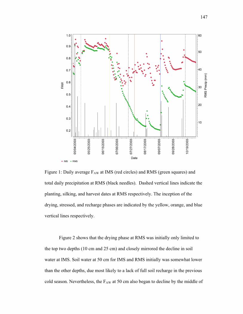
147
Figure 1: Daily average FAW at IMS (red circles) and RMS (green squares) and
total daily precipitation at RMS (black needles). Dashed vertical lines indicate the
planting, silking, and harvest dates at RMS respectively. The inception of the
drying, stressed, and recharge phases are indicated by the yellow, orange, and blue
vertical lines respectively.
Figure 2 shows that the drying phase at RMS was initially only limited to
the top two depths (10 cm and 25 cm) and closely mirrored the decline in soil
water at IMS. Soil water at 50 cm for IMS and RMS initially was somewhat lower
than the other depths, due most likely to a lack of full soil recharge in the previous
cold season. Nevertheless, the FAW at 50 cm also began to decline by the middle of

148
the drying phase, albeit at a more accelerated rate at RMS than at IMS, where
irrigation treatments prevented further decline. By the end of the drying phase, soil
water at 100 cm had begun to be depleted at RMS and was significant by the
commencement of the stressed phase. Thus, a great divergence in FAW between
RMS and IMS at all four depths was evident by the end of the drying phase and
this difference in soil water availability led to stark differences in ET and GPP
accumulation (Fig. 3) and eventually in grain yield (Suyker and Verma, 2008;
Suyker and Verma, 2009; Suyker and Verma, 2012). The difference in ET rates
caused by water stress is illustrated further by the ratio of RMS ET to IMS ET in
Figure 4. The ratio started decreasing slightly when FAW at RMS fell to 0.5 and
continued to decrease at this rate until FAW was 0.3. The daily rates of ET at RMS
relative to the well-watered IMS became very significant once FAW fell below 0.3,
which resembles the soil water-ET relationship reported in Waring and Running
(1998).
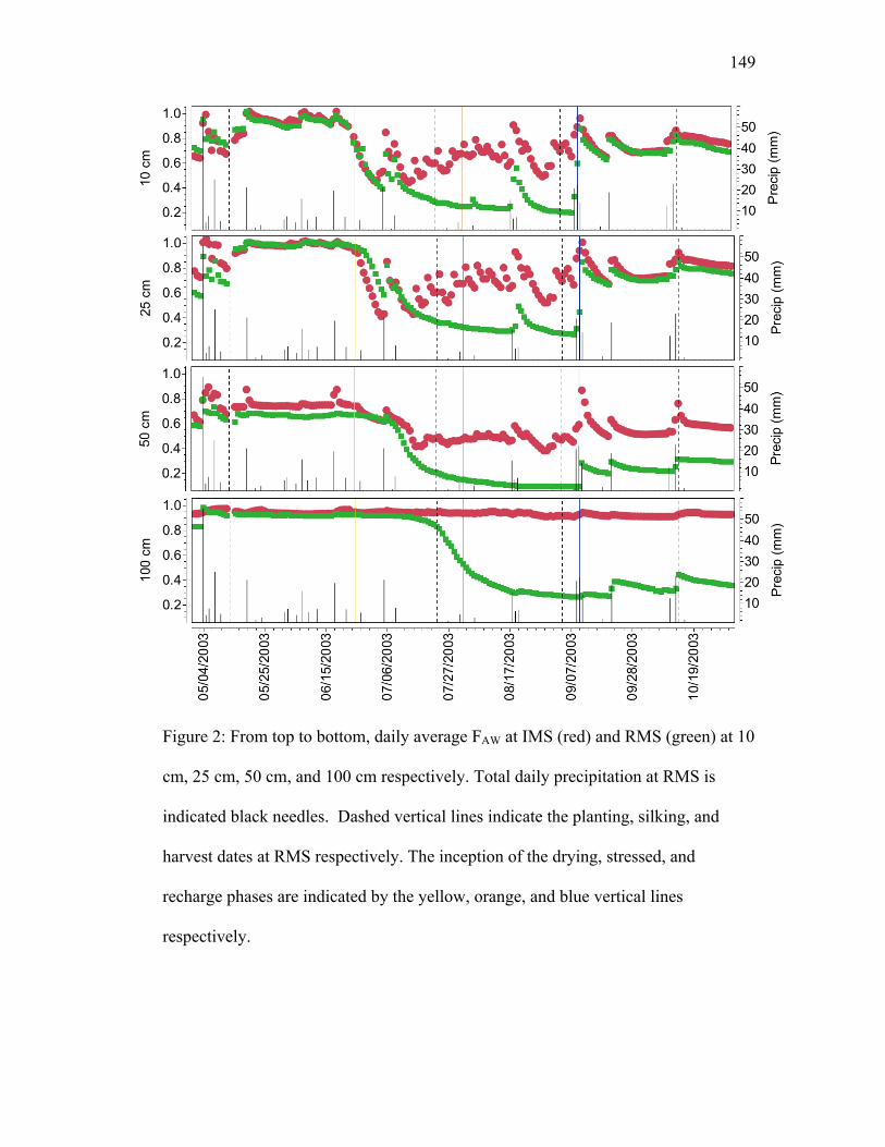
149
Figure 2: From top to bottom, daily average FAW at IMS (red) and RMS (green) at 10
cm, 25 cm, 50 cm, and 100 cm respectively. Total daily precipitation at RMS is
indicated black needles. Dashed vertical lines indicate the planting, silking, and
harvest dates at RMS respectively. The inception of the drying, stressed, and
recharge phases are indicated by the yellow, orange, and blue vertical lines
respectively.
150
Figure 3: Accumulated evapotranspiration (top) and gross primary productivity at
IMS (red) and RMS (green). Dashed vertical lines indicate the planting, silking, and
harvest dates at RMS respectively. The inception of the drying, stressed, and
recharge phases are indicated by the yellow, orange, and blue vertical lines
respectively.
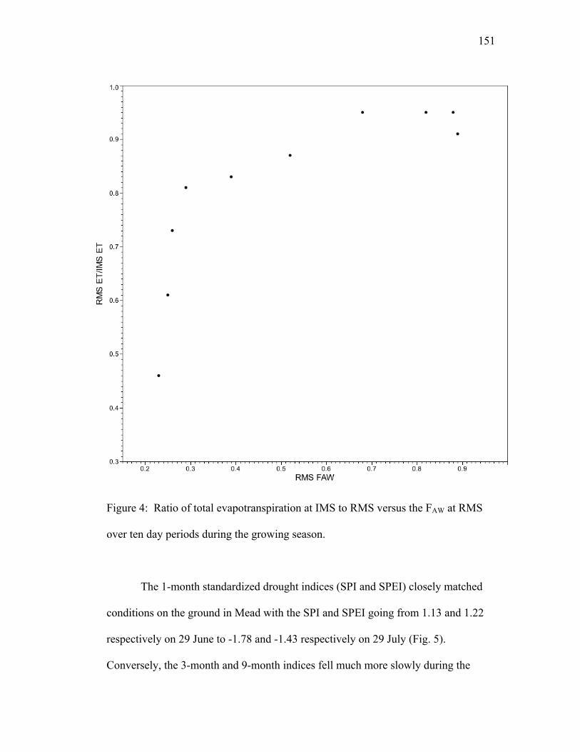
151
Figure 4: Ratio of total evapotranspiration at IMS to RMS versus the FAW at RMS
over ten day periods during the growing season.
The 1-month standardized drought indices (SPI and SPEI) closely matched
conditions on the ground in Mead with the SPI and SPEI going from 1.13 and 1.22
respectively on 29 June to -1.78 and -1.43 respectively on 29 July (Fig. 5).
Conversely, the 3-month and 9-month indices fell much more slowly during the

152
drying phase and were significantly higher than the 1-month indices by 29 July
(Fig. 5). For example, while the 1-month SPI (SPEI) had fallen to -1.78 (-1.43) on
29 July, the 3-month SPI had only dropped to 0.06 (0.19). The 9-month SPI and
SPEI were somewhat more indicative of the drying phase by 29 July, but that was
as much a result of dry conditions early in the 9-month period than the drought that
had developed in the preceding weeks.
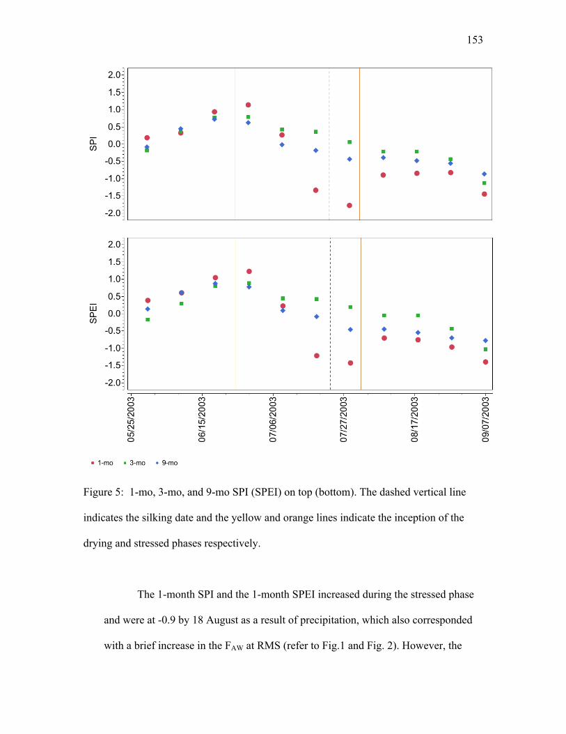
153
Figure 5: 1-mo, 3-mo, and 9-mo SPI (SPEI) on top (bottom). The dashed vertical line
indicates the silking date and the yellow and orange lines indicate the inception of the
drying and stressed phases respectively.
The 1-month SPI and the 1-month SPEI increased during the stressed phase
and were at -0.9 by 18 August as a result of precipitation, which also corresponded
with a brief increase in the FAW at RMS (refer to Fig.1 and Fig. 2). However, the
154
magnitude of the increase in the 1-month indices was partly a result of an
additional 20 mm of precipitation falling at nearby Lincoln, NE than at RMS in the
period from 31 July to 4 August. Therefore, it is likely that the 1-month SPI and
SPEI were somewhat underestimating the severity of the dryness during the
stressed phase at RMS, which in turn demonstrates the main disadvantage of using
a nearby weather station as a proxy for meteorological data when calculating a
drought index.
The remainder of this section of the paper is setup to look at the
relationship of these parameters (i.e., soil water, ET, GPP) during individual phases
in more detail. Since the first three phases coincided with maize being in the
vegetative and/or reproductive stages, soil water (both composite and by individual
depth), ET accumulation, and GPP accumulation at RMS are compared with IMS.
The recharge phase occurred after maize at RMS had reached maturity and thus
only soil water comparisons are applicable. The 1-mo and 9-mo drought indices
(i.e., SPI and SPEI) are also discussed during the subsections for the individual
phases (except the recharge phase).
3.2 Moist phase
Significant precipitation fell over the region about ten days before planting,
which led to an increase in FAW at both sites and elimination of the difference in
FAW between the two sites at 100 cm (Fig. 6). Adequate precipitation during the
rest of the moist phase allowed for a nearly identical FAW at 10, 25, and 100 cm and
only slightly higher FAW at IMS than RMS at 50 cm. Equivalent amounts of soil
water between the two sites led to nearly identical daily rates of ET, with IMS
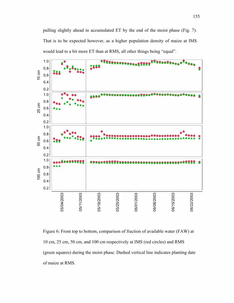
155
pulling slightly ahead in accumulated ET by the end of the moist phase (Fig. 7).
That is to be expected however, as a higher population density of maize at IMS
would lead to a bit more ET than at RMS, all other things being “equal”.
Figure 6: From top to bottom, comparison of fraction of available water (FAW) at
10 cm, 25 cm, 50 cm, and 100 cm respectively at IMS (red circles) and RMS
(green squares) during the moist phase. Dashed vertical line indicates planting date
of maize at RMS.
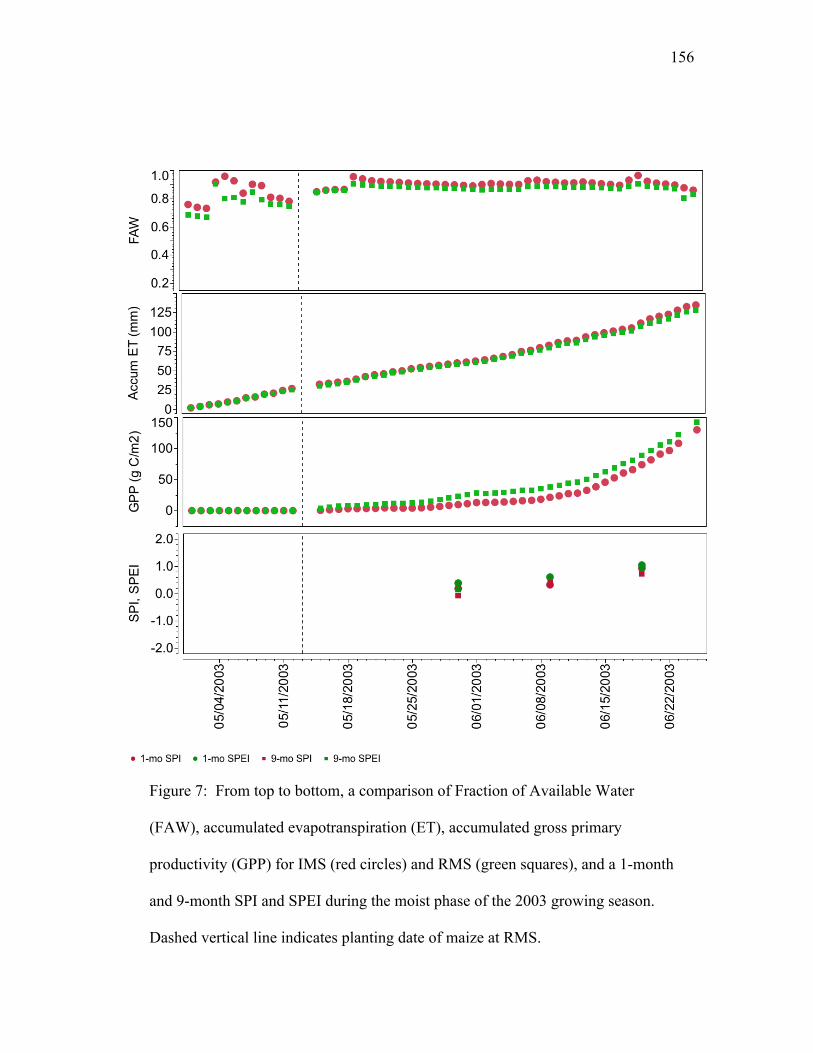
156
Figure 7: From top to bottom, a comparison of Fraction of Available Water
(FAW), accumulated evapotranspiration (ET), accumulated gross primary
productivity (GPP) for IMS (red circles) and RMS (green squares), and a 1-month
and 9-month SPI and SPEI during the moist phase of the 2003 growing season.
Dashed vertical line indicates planting date of maize at RMS.
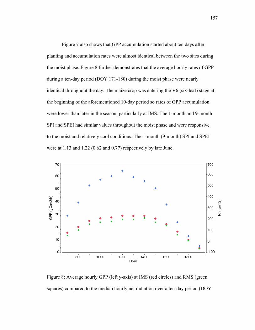
157
Figure 7 also shows that GPP accumulation started about ten days after
planting and accumulation rates were almost identical between the two sites during
the moist phase. Figure 8 further demonstrates that the average hourly rates of GPP
during a ten-day period (DOY 171-180) during the moist phase were nearly
identical throughout the day. The maize crop was entering the V6 (six-leaf) stage at
the beginning of the aforementioned 10-day period so rates of GPP accumulation
were lower than later in the season, particularly at IMS. The 1-month and 9-month
SPI and SPEI had similar values throughout the moist phase and were responsive
to the moist and relatively cool conditions. The 1-month (9-month) SPI and SPEI
were at 1.13 and 1.22 (0.62 and 0.77) respectively by late June.
Figure 8: Average hourly GPP (left y-axis) at IMS (red circles) and RMS (green
squares) compared to the median hourly net radiation over a ten-day period (DOY
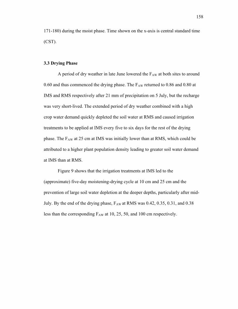
158
171-180) during the moist phase. Time shown on the x-axis is central standard time
(CST).
3.3 Drying Phase
A period of dry weather in late June lowered the FAW at both sites to around
0.60 and thus commenced the drying phase. The FAW returned to 0.86 and 0.80 at
IMS and RMS respectively after 21 mm of precipitation on 5 July, but the recharge
was very short-lived. The extended period of dry weather combined with a high
crop water demand quickly depleted the soil water at RMS and caused irrigation
treatments to be applied at IMS every five to six days for the rest of the drying
phase. The FAW at 25 cm at IMS was initially lower than at RMS, which could be
attributed to a higher plant population density leading to greater soil water demand
at IMS than at RMS.
Figure 9 shows that the irrigation treatments at IMS led to the
(approximate) five-day moistening-drying cycle at 10 cm and 25 cm and the
prevention of large soil water depletion at the deeper depths, particularly after mid-
July. By the end of the drying phase, FAW at RMS was 0.42, 0.35, 0.31, and 0.38
less than the corresponding FAW at 10, 25, 50, and 100 cm respectively.
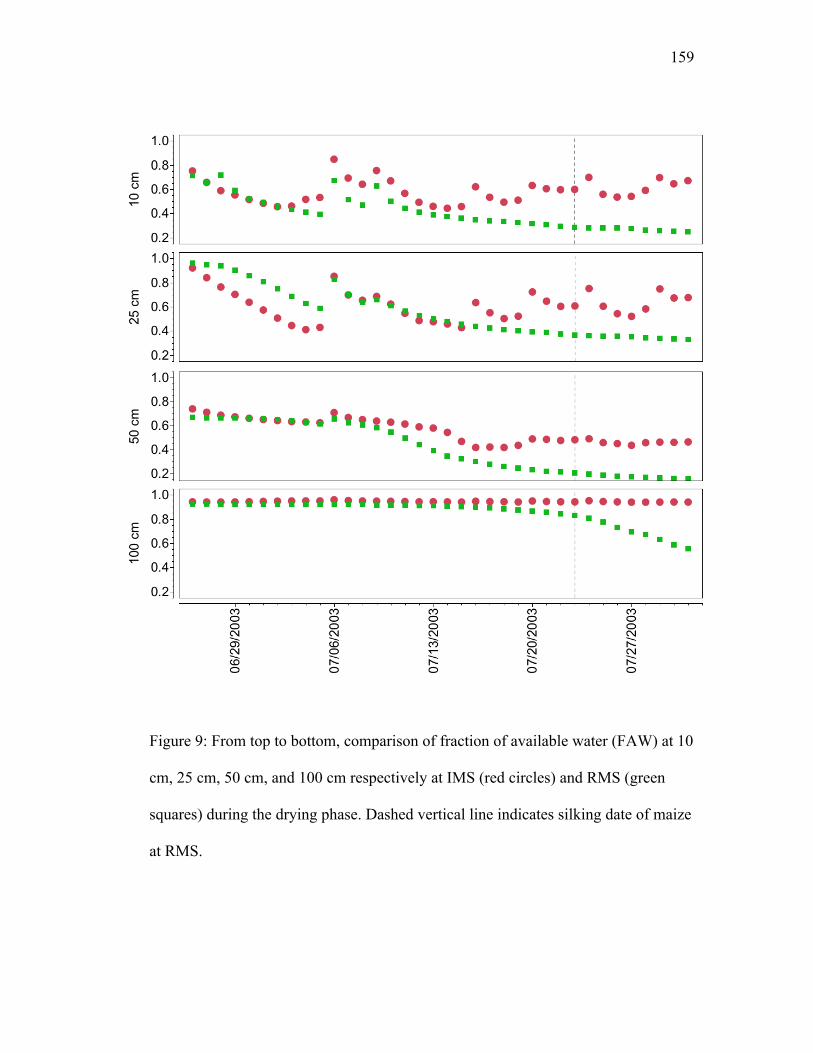
159
Figure 9: From top to bottom, comparison of fraction of available water (FAW) at 10
cm, 25 cm, 50 cm, and 100 cm respectively at IMS (red circles) and RMS (green
squares) during the drying phase. Dashed vertical line indicates silking date of maize
at RMS.
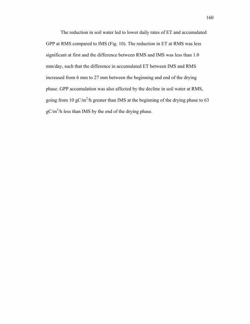
160
The reduction in soil water led to lower daily rates of ET and accumulated
GPP at RMS compared to IMS (Fig. 10). The reduction in ET at RMS was less
significant at first and the difference between RMS and IMS was less than 1.0
mm/day, such that the difference in accumulated ET between IMS and RMS
increased from 6 mm to 27 mm between the beginning and end of the drying
phase. GPP accumulation was also affected by the decline in soil water at RMS,
going from 10 gC/m2/h greater than IMS at the beginning of the drying phase to 63
gC/m2/h less than IMS by the end of the drying phase.
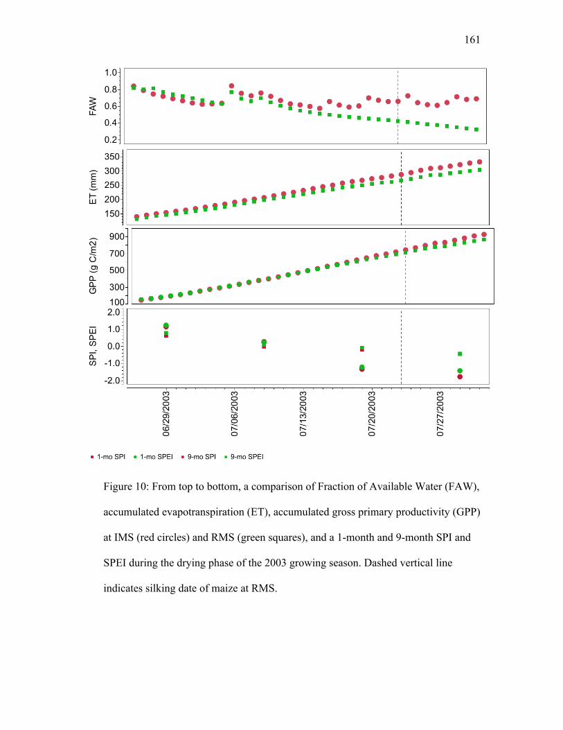
161
Figure 10: From top to bottom, a comparison of Fraction of Available Water (FAW),
accumulated evapotranspiration (ET), accumulated gross primary productivity (GPP)
at IMS (red circles) and RMS (green squares), and a 1-month and 9-month SPI and
SPEI during the drying phase of the 2003 growing season. Dashed vertical line
indicates silking date of maize at RMS.

162
Plants under water stress close stomata as a direct signal from the metabolic
activity of roots under water stress (Schulze 1986). Thus, the reduction in ET and
GPP at RMS implies stomatal conductance of maize at RMS was reduced
compared to that of maize at IMS. Figure 11 adds validation to this by showing the
divergence in average hourly GPP at RMS compared to that of IMS during peak
hours of peak net radiation over a ten-day period (DOY 201-210) in the drying
phase. For example, during the hour ending at 1100 LST, the average GPP
accumulations at IMS and RMS were 67 and 51 gC/m2/h respectively. Maize was
entering the reproductive stage at both sites during this period and thus, hourly
GPP accumulation was much more significant than during the ten-day period in the
moist phase.
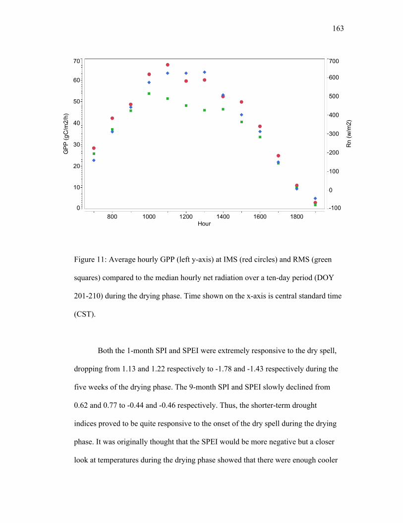
163
Figure 11: Average hourly GPP (left y-axis) at IMS (red circles) and RMS (green
squares) compared to the median hourly net radiation over a ten-day period (DOY
201-210) during the drying phase. Time shown on the x-axis is central standard time
(CST).
Both the 1-month SPI and SPEI were extremely responsive to the dry spell,
dropping from 1.13 and 1.22 respectively to -1.78 and -1.43 respectively during the
five weeks of the drying phase. The 9-month SPI and SPEI slowly declined from
0.62 and 0.77 to -0.44 and -0.46 respectively. Thus, the shorter-term drought
indices proved to be quite responsive to the onset of the dry spell during the drying
phase. It was originally thought that the SPEI would be more negative but a closer
look at temperatures during the drying phase showed that there were enough cooler
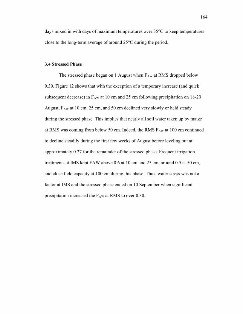
164
days mixed in with days of maximum temperatures over 35°C to keep temperatures
close to the long-term average of around 25°C during the period.
3.4 Stressed Phase
The stressed phase began on 1 August when FAW at RMS dropped below
0.30. Figure 12 shows that with the exception of a temporary increase (and quick
subsequent decrease) in FAW at 10 cm and 25 cm following precipitation on 18-20
August, FAW at 10 cm, 25 cm, and 50 cm declined very slowly or held steady
during the stressed phase. This implies that nearly all soil water taken up by maize
at RMS was coming from below 50 cm. Indeed, the RMS FAW at 100 cm continued
to decline steadily during the first few weeks of August before leveling out at
approximately 0.27 for the remainder of the stressed phase. Frequent irrigation
treatments at IMS kept FAW above 0.6 at 10 cm and 25 cm, around 0.5 at 50 cm,
and close field capacity at 100 cm during this phase. Thus, water stress was not a
factor at IMS and the stressed phase ended on 10 September when significant
precipitation increased the FAW at RMS to over 0.30.
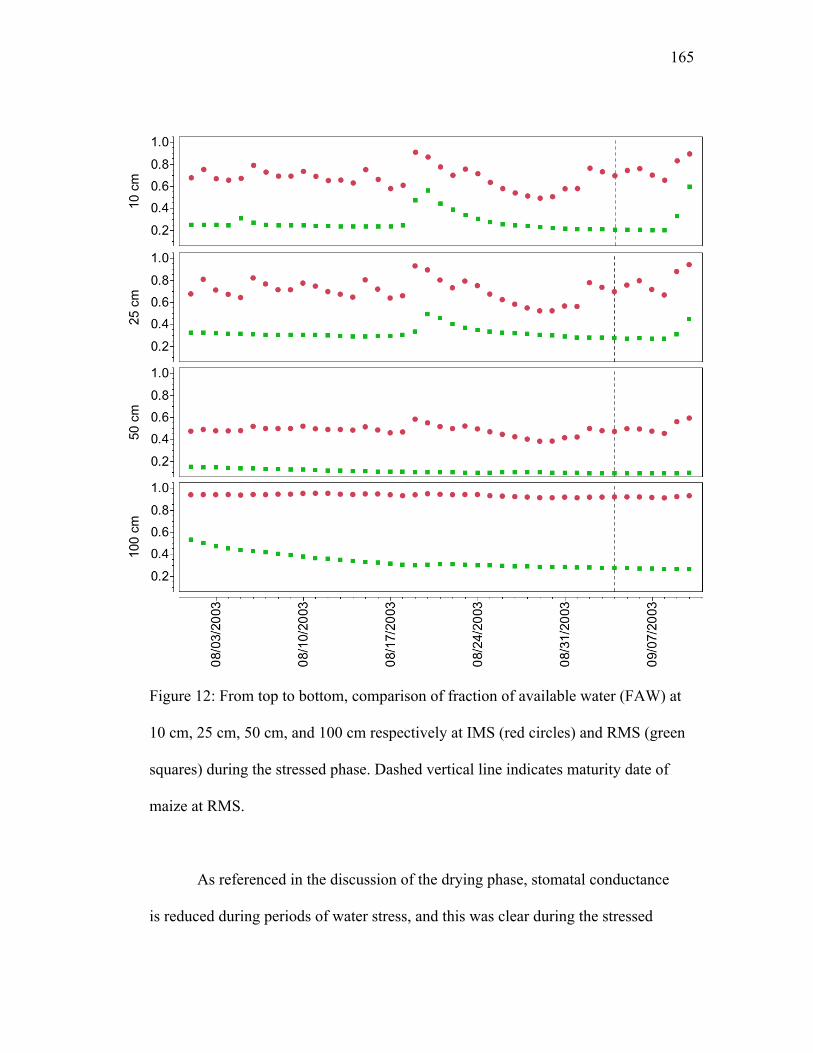
165
Figure 12: From top to bottom, comparison of fraction of available water (FAW) at
10 cm, 25 cm, 50 cm, and 100 cm respectively at IMS (red circles) and RMS (green
squares) during the stressed phase. Dashed vertical line indicates maturity date of
maize at RMS.
As referenced in the discussion of the drying phase, stomatal conductance
is reduced during periods of water stress, and this was clear during the stressed

166
phase at RMS. Daily ET rates widened further in the stressed phase as IMS
averaged 4.8 mm/day and RMS averaged 3.1 mm/day, such that a difference of 94
mm existed by the end of the stressed phase (Fig. 13). GPP was also greatly
affected and the difference in accumulated GPP increased to 294 gC/m2 between
IMS and RMS during the stressed phase. Perhaps the most striking evidence of
reduced stomatal conductance comes from Figure 14. At well-watered IMS, the
average hourly accumulation over a ten-day period (DOY 221-230) closely follows
the net radiation curve and peaks at 1100 CST at 62 gC/m2, indicating that little to
no stress was put on the crop (i.e., little to no inhibition on photosynthesis).
Meanwhile at the water-stressed RMS, hourly GPP accumulation began to level
out early in the morning and peaked at 46 gC/m2 at 1100 CST, adding more
evidence of water stress significantly reducing stomatal conductance.
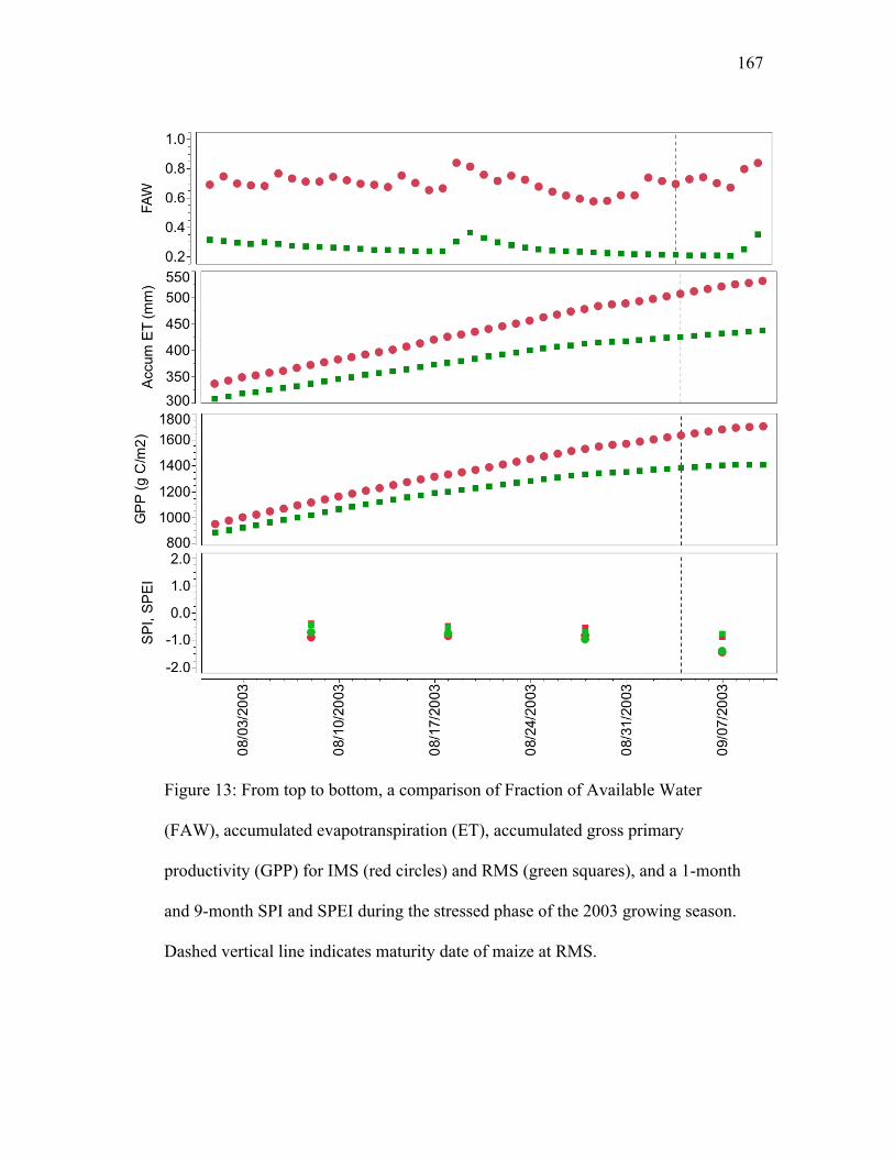
167
Figure 13: From top to bottom, a comparison of Fraction of Available Water
(FAW), accumulated evapotranspiration (ET), accumulated gross primary
productivity (GPP) for IMS (red circles) and RMS (green squares), and a 1-month
and 9-month SPI and SPEI during the stressed phase of the 2003 growing season.
Dashed vertical line indicates maturity date of maize at RMS.
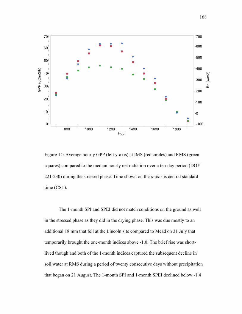
168
Figure 14: Average hourly GPP (left y-axis) at IMS (red circles) and RMS (green
squares) compared to the median hourly net radiation over a ten-day period (DOY
221-230) during the stressed phase. Time shown on the x-axis is central standard
time (CST).
The 1-month SPI and SPEI did not match conditions on the ground as well
in the stressed phase as they did in the drying phase. This was due mostly to an
additional 18 mm that fell at the Lincoln site compared to Mead on 31 July that
temporarily brought the one-month indices above -1.0. The brief rise was short-
lived though and both of the 1-month indices captured the subsequent decline in
soil water at RMS during a period of twenty consecutive days without precipitation
that began on 21 August. The 1-month SPI and 1-month SPEI declined below -1.4
169
shortly after the onset of physiological maturity (4 September; DOY 247) and the
9-month SPI and SPEI declined steadily over the last month of the stressed phase
to -0.87 and -0.78 respectively. Therefore, the 9-month SPI and SPEI were
somewhat more indicative of the flash drought by the end of the stressed phase
than they had been at the end of the drying phase.
3.5 Recharge phase
Significant precipitation did return to Mead as 56 mm fell over a three-day
period from 9 to 11 September. It was too late to rejuvenate the maize at RMS
unfortunately as physiological maturity had been achieved days earlier. However,
Figure 15 shows that the precipitation from 9-11 September brought the 10 cm FAW
at IMS to near field capacity and the FAW at RMS to 0.87. Significant recharge also
occurred at 25 cm as field capacity was realized at IMS and the FAW at RMS
increased to 0.85. Some recharge also occurred at 50 cm, though there was still a
very large difference in FAW between IMS and RMS.
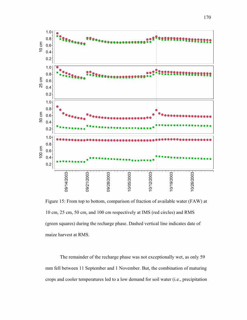
170
Figure 15: From top to bottom, comparison of fraction of available water (FAW) at
10 cm, 25 cm, 50 cm, and 100 cm respectively at IMS (red circles) and RMS
(green squares) during the recharge phase. Dashed vertical line indicates date of
maize harvest at RMS.
The remainder of the recharge phase was not exceptionally wet, as only 59
mm fell between 11 September and 1 November. But, the combination of maturing
crops and cooler temperatures led to a low demand for soil water (i.e., precipitation
171
at RMS was greater than ET) and this was sufficient to keep 10 cm and 25 cm
moist at both sites. It also permitted some additional recharge at 50 cm at both IMS
and RMS and at 100 cm at RMS. Perhaps the most interesting aspect of Figure 15
is how the time series of FAW at 10 cm and 25 cm in the recharge phase resembles
that of the moist phase, as the difference in FAW was minimal between IMS and
RMS. Conversely, the time series of FAW at 50 cm and 100 cm more closely
resembles that of the stressed phase, as large differences in FAW between IMS and
RMS remained, even with some recharge at RMS. Thus, true recharge only
occurred at 10 cm and 25 cm at Mead in 2003, even though there was improvement
at the deeper depths.
4.0 Conclusions
The grain yield of 7.7 Mg/ha at RMS in 2003 was only a little more than
half of the grain yield at IMS (14.0 Mg/ha). For the sake of comparison, during the
more optimal 2009 growing season, RMS had a final grain yield of 12.0 Mg/ha
(Table 1). While it is doubtful that the final yield at RMS would have equaled the
yield of IMS had the 2003 season remained moist, the yield in 2009 gives a useful
comparison for how much yield was potentially lost to the flash drought in 2003.
The term flash drought is appropriate for this case study for two key reasons. The
first reason is precipitation was adequate and soils were moist for the first two
months post-maize planting, which led to comparable rates of ET and GPP
accumulation between IMS and RMS during the moist phase of the season. Thus,
the initiation of drought was well-defined by actual measurements of precipitation
and other agro-meteorological variables.
172
The second reason is that a prolonged stretch with minimal precipitation
occurred during the most critical growth stages for maize and coincided with the
drying and stressed phases discussed earlier. It can be implied that the lack of
precipitation and decline in soil water at RMS led to corresponding decreases in
stomatal conductance, which in turn led to reductions in photosynthesis as
evidenced by the significant differences in GPP accumulation, total ET, and final
grain yield between RMS and IMS. In contrast, when precipitation was adequate
and soil water differences between the two sites were negligible in the moist phase,
both sites had nearly identical levels of accumulated ET.
The difference in accumulated ET and GPP between IMS and RMS
widened considerably after early August, which closely coincides with the period
where soil water at 100 cm went from a linear decrease to a more curvilinear
decrease. The timing of the water stress was critical at RMS as the low decline in
the ET rate that occurred as maize began silking (23 July; DOY 204) accelerated as
maize went through the critical reproductive stage. The irrigated maize at IMS had
no discernible water stress and ET rates remained steady throughout the
reproductive stage. Significant impacts were therefore realized because of the
timing of the drought at RMS. Thus, it can be stated that a flash drought can by
characterized by, but not limited to, a well-defined inception with severe impacts
on vegetation, including grain crops such as maize, and can be of relatively short
duration if a recovery period occurs within a few months of the drought’s
inception.
173
This study also confirmed the effectiveness of using a 1-month SPEI and a
1-month SPI for purposes of flash drought detection. Results showed that both 1-
month indices were robust at detecting the onset of the flash drought (i.e., in the
drying phase) when compared with the 9-month indices as they matched the
decline of soil water at RMS very well. The two indices were close throughout the
season, indicating that temperatures were close to historical averages over the
course of the growing season. While there were indeed several days of
temperatures over 35°C in the 2003 growing season, the 2003 season overall was
not an excessively hot summer by standards of the western U.S. Corn Belt, and
thus the SPEI was not necessarily a better indicator of the flash drought in this
study. However, the SPEI yields vital information about the effect of temperature
in a drought, and it is likely that the SPEI will be a more robust indicator of
drought than the SPI in some future studies. Future work will also be needed to
determine if the relationship between indices calculated over different time scales
(i.e., 1-month, 9-months, etc…) are similar to what was reported in this study.
5.0 Acknowledgements:
The research presented here was supported by the Office of Science (BER), U.S.
Department of Energy Grant (No. DE-FG02-03ER63639 and the University of Nebraska-
Lincoln Program of Excellence. Special thanks to Todd Schimelfenig, Dave Scoby, and
Glen Roebke for providing technical expertise and data.
174
6.0 References:
Abramowitz, M., Stegun, I., 1965. Handbook of Mathematical Functions. Dover
Publications, New York.
Baldocchi, D.D., Hicks, B.B., Meyers, T.P., 1988. Measuring biosphere-atmosphere
exchanges of biologically related gases with micrometeorological methods. Ecology 69
(5), 1331-1340.
Baldocchi, D.D., 2003. Assessing the eddy covariance technique for evaluating carbon
dioxide exchange rates of ecosystems: past, present, and future. Global Change Biol. 9
(4), 479-492.
Basara, J.B., Arndt, D.S., Johnson, H.L., Brotzge, J.G., Crawford, K.C.,1998: An analysis
of the drought of 1998 using the Oklahoma Mesonet. EOS Trans., AGU, 79, 258.
Brown, J.F., Wardlow, B.D., Tadesse, T., Hayes, M.J., Reed, B.C., 2008. The
Vegetartion Drought Response Index (VegDRI): A new integrated approach for
monitoring drought stress in vegetation. GISci. and Rem. Sens. 45: 16-46.
Cakir, R., 2004. Effect of water stress at different development stages on vegetative and
reproductive growth of corn. Field Crops Res. 89, 1-16.
Calvino, P.A., F.H. Andrade, V.O. Sadras, 2003. Maize yield as affected by water
availability, soil depth, and crop management. Agron. J. 95, 275-281.
175
Dale, R. F., Shaw, R.H., 1965. Effect on corn yields of moisture stress and stand at two
different fertility levels. Agron. J. 57, 475-479.
Denmead, O. T., Shaw, R.H., 1960. The effects of soil moisture stress at different stages
of growth on the development and yield of corn. Agron. J. 52, 272-274.
Earl, H. J., Davis, R.F., 2003. Effect of drought stress on leaf and whole canopy maize
radiation use efficiency and yield of maize. Agronomy Journal 95: 688-696.
Guttman, N. B., 1998. Comparing the Palmer Drought Index and the Standardized
Precipitation Index. J. Amer. Water Resour. Assoc., 34, 113–121.
Guttman, N.B., 1999. Accepting the Standardized Precipitation Index: A calculation
algorithm. J. Amer. Water Resour. Assoc., 35, 311-322.
Hayes, M., D. A. Wilhite, M. Svoboda, and O. Vanyarkho. 1999. Monitoring the 1996
drought using the standardized precipitation index. Bull. Amer. Meteor. Soc., 80, 429–
438.
Hayes, M., M. Svoboda, N. Wall, M. Widhalm, 2011. The Lincoln declaration on
drought indices: Universal meteorological drought index recommended. Bull. Amer.
Meteor. Soc.,92, 485-488.
176
Heim, R. R., 2002: A review of twentieth-century drought indices used in the United
States. Bull. Amer. Meteor. Soc., 83, 1149–1165.
Hillel, D., 2004. Introduction to Environmental Soil Physics. Elsevier Academic Press,
San Diego.
Hollinger, S. E. and S. A. Isard, 1994. A soil moisture climatology of Illinois. J. Climate
7, 822-833.
Hosking, J.R.M., 1990. L-Moments: Analysis and estimation distributions using linear
combinaitons of order statistics. J.R. Statist. Soc. 52 (1), 105-124.
Hu, Q., G. D. Willson. 2000. Effect of temperature anomalies on the Palmer drought
severity index in the central United States. Int. J. Climatol., 20, 1899–1911.
Hubbard, K.G., 1994. Spatial variability of weather variables in the high plains of the
USA. Agric. For. Meteor. 68, 29-41.
Hubbard, K.G., DeGaetano, A.T., Robbins, K.D., 2004. A modern applied climate
information system. Bull. Amer. Meteorol. Soc. 85 (6), 811-812.
177
Hubbard, K.G., You, J., Sridhar, V., Hunt, E., Korner, S., Roebke, G., 2009. Near-surface
soil water monitoring for water resources management on a wide-area basis in the Great
Plains. Great Plains Res., 19, 45-54.
Illston, B.G., Basara, J.B., 2003. Analysis of short-term droughts in Oklahoma. Eos.
Trans. AGU: 84 (17), 157.
Illston, B.G., Basara, J.B., Crawford, K.C., 2004. Seasonal to interannual variations of
soil moisture measured in Oklahoma. Int. J. Climatol. 24, 1883-1896.
Illston, B. G., Basara, J.B., Fischer, D.K., Elliott, R.L., Fiebrich, C., Crawford, K.S.,
Humes, K., Hunt, E. 2008. Mesoscale monitoring of soil moisture across a statewide
network. J. Atmos. and Oceanic Tech. 25, 167-182.
Livida, I., Assemakopoulos, V.D. 2007. Spatial and temporal analysis of drought in
Greece using the Standardized Precipitation Index (SPI). Theoret. Appl. Climatol. 89,
143-153.
Lloyd-Hughes, B., M. A. Saunders. 2002. A drought climatology for Europe. Int. J.
Climatol., 22, 1571–1592.
178
McKee, T. B., Doesken, N.J., Kleist, J., 1993. The relationship of drought frequency and
duration to time scales. Preprints, Eighth Conf. on Applied Climatology. Anaheim, CA,
Amer.
Meteor. Soc., 179–184.
McRoberts, B., Nielsen-Gammon, J. 2012. The Use of a High-Resolution Standardized
Precipitation Index for Drought Monitoring and Assessment. J. Appl. Met. Climatol. 51
(1), 68-83.
Mavromatis, T., 2007. Drought index evaluation for assessing future wheat production in
Greece. Int. J. Climatol., 27 (7), 911-924.
Meyer, S.J., Hubbard, K.G., Wilhite, D.A., 1993. A crop-specific drought index for corn:
I. Model development and validation. Agron J., 85, 388-395.
Monteith, J.L., 1964. Evaporation and environment. The State and Movement of Water in
Living Organisms, 19th Symp. Soc. Biol., Academic Press, NY, pp. 205-234.
Nield, R.E., Newman, N.E., 1990. Growing season characteristics and requirements in
the Corn Belt. National Corn Handbook, Purdue University, Cooperation Extension
Service, West Lafayette, IN.
Palmer, W. C., 1965. Meteorological droughts. U.S. Department of Commerce, Weather
Bureau Research Paper 45, 58 pp.
179
Peterson, T.C., Easterling, WD.R., Karl, T.A., Groisman, P., Nicholls, N., Plummer, N.,
Torok, S., Auer, I., Boehm, R., Gullett, D., Vincent, L., Heino, R., Tuomenvirta, H.,
Mestre, O., Szentimrey, T., Salinger, J., Forland, Hanssen-Bauer, I., Alexandersson, H.,
Jones, P., Parker, D. 1998. Homogeneity adjustments of in situ atmospheric climate data:
A review. Int. J. Climatol., 18: 1493-1517.
Schulze, E.D., 1986. Carbon dioxide and water vapor exchange on response to drought in
the atmosphere and in the soil. Ann. Rev. Plant Physiol. 37, 247-274.
Scott, R.W., Krug, E.C., Burch, S.L., 2010 Illinois soil moisture under sod experiment. J.
Hydromet., 11: 683-704.
Suyker, A.E., Verma, S.B., Burba, C.G., 2003. Interannual variability in net CO2
exchange of a native tallgrass prairie. Global Change Biol. 9, 1-11.
Suyker, A. E., Verma, S.B., 2008. Interannual water vapor and energy exchange in an
irrigated maize-based agroecosystem. Agric. For. Meteorol. 148, 417-427.
Suyker, A. E. , Verma, S.B., 2009. Evapotranspiration of irrigated and rainfed maize-
soybean cropping systems. Agric. For. Meteorol. 149, 443-452.
180
Suyker, A.E., Verma, S.B., 2012. Gross primary production and ecosystem respiration of
irrigated and rainfed maize-soybean cropping system over 8 years. Agric. For. Meteorol.
165, 12-24.
Svoboda, M., Lecomte, D., Hayes, M., Heim, R., Gleason, K., Angel, J., Rippey, B.,
Tinker, R., Palecki, M., Stooksbury, D., Miskus, D., Stephens, S., 2002. The Drought
Monitor. Bull. Amer. Meteorol. Soc. 83 (8): 1181-1190.
Thornthwaite, C.W., 1948. An approach toward a rational classification of climate.
Geogr. Rev. 38, 55-94.
Tufekcioglu, A., Raich, J.W., Isenhart, T.M., Schultz, R.C., 1999. Fine root dynamics,
coarse root biomass, root distribution, and soil respiration in a multispecies riparian
buffer in Central Iowa, USA. Agrofor. Sys. 44, 163-174.
Topp, G.C., Davis, J.L. Annan, A.P., 1980. Elecctromagentic determination of soil water
content: measurement in coaxial transmission lines. Water Resour. Res. 16, 574-582.
Verma, S.B., Dobermann, A., Cassman, K.G., Walters, D.T., Knops, J.M., Arkebauer,
T.J., Suyker, A.E., Burba, G.G., Amos, B., Yang, H., Ginting D., Hubbard, K.G.,
Gitelson A.A., Walter-Shea, E., 2005. Annual carbon dioxide exchange in irrigated and
rainfed maize-based agroecosystems. Agric. For. Meteorol. 131, 77-96.
181
Vicente-Serrano, S.M., Begueria, S., Lopez-Moreno, J.I., 2010. A Multiscalar Drought
Index Sensitive to Global Warming: The Standardized Precipitation Evapotranspiration
Index. J Climate 23: 1696-1718.
Waring, R.H. and S.W. Running,1998. Forest Ecosystems: Analysis at Multiple Scales.
Academic Press, New York.
Wilhite, D.A., M.H. Glantz. 1985. Understanding the drought phenomenon: The role of
definitions. Water Int., 10, 111-120.
Wu, H., Hayes, M.J., Wilhite, D.A., Svoboda, M.D., 2005. The effect of length of record
on the standardized precipitation index calculation. Int. J. Climatol. 25 (4), 505-520.
Xu, L., Baldocchi, D.D., 2004. Seasonal variation in carbon dioxide exchange over a
Mediterranean annual grassland in California. Agric. For. Meterol. 113 (1-4), 223-243.
You, J., K.G. Hubbard, Mahmood, R., Srihar, V., Todey, D., 2010. Quality control of soil
water data in Applied Climate Information System - case study in Nebraska. J. Hydrol.
Eng. 15, 200-209.
182
CHAPTER 5: CONCLUSIONS
Eight years of soil moisture and biophysical data from the Carbon
Sequestration Project (CSP) provided valuable insights into the inter-relatioship of
soil moisture and plant response of corn under varying climatic growing season
conditions and the location of these field sites. In addition, the location of these
field sites in the transitional zone between the semi-arid High Plains and the wetter
sub-humid Corn Belt to the east allowing for the lessons learned from this work to
be expand to other parts of these adjacent regions. While it is impossible to totally
simulate soil water and biophysical behavior of maize and/or soybeans for another
location with data from the CSP sites, the wide range of conditions during the
eight-year study period couple with its transitional zone location can give us
insight as to the interactions of soil moisture and biophysical variables such as
evapotranspiration and gross primary productivity under varying climatic
conditions.
For example, the conditions for most of the latter half of the 2003 growing
season could be a good proxy for rainfed maize grown under typical conditions of
a semi-arid location like the Nebraska panhandle because total precipitation in July
and August was less than a typical July and August in Scottsbluff. Conversely, the
2009 season could be a good proxy for a typical season for a maize crop grown in
northeast Iowa because of seasonal average temperatures that were more than 2°C
below the 30-year average and growing season precipitation that was above
average at Mead. The eight-year study period at Mead captured some of the wettest
and driest periods of the past 30+ years for this location and therefore, the data
183
shown in this dissertation captures the majority(~95%) of the historical
agroclimatological range of temperature and precipitation.
As mentioned numerous times throughout the research chapters, soil
moisture is a critical parameter for the Earth’s hydrological balance, in part due to
its necessity for stomatal conductance to remain high. Soil moisture varied within
and between season and none of the seasons in the study period were 100% moist
(i.e., no days of stress) or 100% dry (i.e., all days were in stress). However, there
was a marked difference in soil moisture between the beginning (2002-2005) and
end (2006-2009) of the study period. From 2002-2005, precipitation was
consistently below the 30-year median in every growing season and there were
prolonged periods of drought stress. Dry spells and subsequent soil water depletion
had detrimental impact on yields at the rainfed site (RMS) compared to the
irrigated site (IMS), particularly during the 2003 flash drought when the maize
yield at RMS was slightly more than half of that at IMS. The climatic growing
season conditions during these years demonstrate the benefit of irrigation at a
western Corn Belt site like Mead and the necessity of it in a semi-arid environment
where seasons are typically like those in the first half of the study period at Mead.
Conversely, precipitation was generally above average over the study sites
in the latter part of study period starting after mid-summer in 2006. As documented
in earlier chapters, drier spells and soil moisture depletion (particularly at the top
soil layer depth) at times during the latter part of the study period, but the
magnitude of depletion was lower and the duration much shorter than during the
earlier years of the study period. Irrigation water applications were less numerous
184
at IMS and yields at RMS were closer to those of IMS, particularly in 2009 (maize)
when there were no days of stress at 50 cm and in 2006 when significant
precipitation was well-timed for the soybean production.
One of the goals of the dissertation was to show that timing of precipitation
during the growing season (GS) is equally as important as the total precipitation.
For example, chapter 3 showed that yield for the maize crop in 2005, which
received precipitation well-below the 30-year median that growing, had yields at
the rainfed site (RMS) that was only about 1.0 Mg/ha less than in 2007, despite the
seasonal precipitation being over 300 mm lower. The timing of precipitation was
particularly important for irrigation scheduling at IMS. The years with the fewest
irrigation application for both maize and soybeans were not the wettest years
during the study period. Paradoxically, the year with the fewest irrigation
treatments when soybeans were the common crop (2006), had below-average GS
precipitation. The year with the most irrigation treatments when soybeans were the
common crop (2008) was one of the wettest seasons in the 30-year POR. The
difference between the below average 2006 GS and the wet 2008 GS is that
precipitation fell at regular intervals during the critical growth period (July and
August) for soybeans in 2006 and kept the soil profile moist. In comparison, the
only dry spell of the 2008 GS occurred during that same critical period, thus
necessitating irrigation applications that prevented depletion of the top half of the
soil moisture profile within the root zone of soybeans at IMS.
For years where maize was the common crop, the wettest GS (2007) did not
have the highest average soil moisture across all depths or the highest yields at
185
RMS. That distinction belonged to the 2009 GS, which was only slightly above
the 30-year median. Again, timing was the key difference. A large share of the
precipitation in the 2007 GS occurred early in the season and then during-late
summer and autumn, which are outside of the critical growth stage that determines
the yield of maize (i.e., silking during mid-summer). The majority of precipitation
in the 2009 GS occurred during the critical stages for maize, keeping the soil
profile moist and achieving higher yields than might be expected with total
precipitation that was only slightly above the 30-year median. Thus, the old adage
that timing is everything, certainly had a strong element of truth in this research
when it came to precipitation, soil moisture, and crop yield.
Another goal of the dissertation was to show the direct effect of soil water
depletion and soil water recharge on measured biophysical parameters such as ET
and GPP. As was expected, total ET and GPP were higher in all seasons at IMS
than at RMS over the entire study period. During the dry spells, soil water stress
often caused noticeable reductions in the daily rates of ET at RMS compared to
IMS, as well as the daily accumulation of GPP and the LE ratio. Collectively, these
results imply that soil water stress reduced stomatal conductance, particularly
during the afternoon hours when water stress was more incipient. However, if the
water stress persisted, as was the case in the 2003 flash drought, the effect was
realized earlier in the day.
In chapter 3, the analysis revealed that rainfed maize does have some
resilience to soil water deficits if precipitation is timely and sufficient in magnitude
for soil water recharge at all depths. Every year that maize was the common crop
186
between RMS and IMS, there was a period when the LE ratio dipped well below
1.0. Also, in every year except 2003, there were significant precipitation events
that moistened the soils at all depths analyzed, which in turn led to a significant
increase in the LE ratio. Thus, it is possible to conclude that a significant recharge
of soil water after incipient water stress can lead to some level of rejuvenation of
the maize crop, via increased stomatal conductance. The best example of this was
in 2005 when soil water depletion led to a large reduction in the LE ratio by the
beginning of the critical period. The LE ratio then increased significantly after a
precipitation event about a week after the onset of silking. That rejuvenation did
not occur in 2003 because of flash drought conditions, which was studied in depth
in chapter 4. The overall goal of it was to compare in situ meteorological data (i.e.,
temperature and precipitation) and biophysical data (i.e., soil moisture, ET, and
GPP) with widely-used drought indices (e.g., SPI) to evaluate effectiveness of the
indices to indicate a short-term agricultural drought conditions, which led to severe
reductions in yield.
Results in Chapter 4 confirmed the effectiveness of using two 1-month
climate indices at characterizing flash drought conditions. The two indices, the
Standardized Precipitation Index (SPI) and the Standardized Precipitation
Evapotranspiration Index (SPEI), are normalized and spatially invariant indices
used to determine drought severity. As discussed in chapter 4, the biggest
difference between the SPI and the SPEI is the temperature dependence of the
SPEI. Thus, a drought combined with well-above average temperatures would be
187
better characterized by the temperature sensitive SPEI more than the precipitation-
only SPI.
In the case of the 2003 flash drought, the two indices differed little
throughout the season, indicating that temperatures were close to historical
averages over the course of the growing season. Thus, there was not conclusive
evidence that the more recently developed SPEI was a better indicator of the flash
drought with the addition of temperature in the index calculation, as was the
original hypothesis. While several days exceeded temperatures over 35°C during
the 2003 growing season, the season as whole was not an excessively hot summer,
and thus the inclusion of a temperature component in the SPEI did not necessarily
make it a better indicator of the flash drought than the precipitation-based SPI.
However, if the effects of climate change produce more intense and “hot”
droughts, it is likely that temperature could be a more pronounced controlling
factor and the SPEI would be a more robust indicator of drought than the SPI.
The primary objective of this dissertation was to show detailed analyses of
soil water under crop cover and its relationship with biophysical variables over an
eight-year period. While the effect of soil water depletion had been previously well
established, the data presented in dissertation are unique in several respects. First,
the soil water and biophysical data came from fields (e.g., RMS) that were over 50
ha in size and managed in a way that is typical for producers in the United States
Corn Belt. Thus, there is potentially more applicability and/or extensibility of the
findings presented earlier in the research chapters for agricultural producers than
188
there would be if the data had come from highly controlled, small experimental
plots.
Another unique aspect of the earlier presented data is the location they
came from and the duration of the period over which they were collected. The CSP
study-sites near the town of Mead, NE are in a true transition zone between rainfed
dominant agroecosytems to the east and predominantly irrigated agroecosystems to
the west. As discussed in chapter 2, the probability of a high yielding rainfed crop
was lower than sites in Iowa and Illinois, but much higher than the other two sites
in western Nebraska. Over the eight years used for analysis in the dissertation, the
conditions at Mead ranged from wetter than the 30-years average for a site in the
Central and Eastern Corn Belt to drier than the 30-year average for a site in the
Nebraska panhandle. It could be argued that the wet periods at Mead could be a
good proxy for the typical soil water-biophysical variable (e.g., ET) relationship of
a maize or soybean crop at a site in the Central and Eastern Corn Belt and the dry
periods could be a good proxy for the typical soil water-biophysical variable
relationship of a maize or soybean crop in a semi-arid site like western Nebraska.
Thus, the Mead CSP site has the potential to be a good “testbed” location for all
types of agro-ecological and agro-economic studies and research.
The information presented in the dissertation has the possibility of being of
high value beyond producers. One of the recommend areas for future research and
work is in the realm of model validation. With land data assimilation systems, such
as the North American Land Data Assimilation System (NLDAS) and the Land
Information Systems (LIS), becoming more widely used and with land surface

189
models having increasingly sophisticated physics options (e.g., the Noah Multi-
Physics model), there will be more demand for validation of outputs like soil
moisture and fluxes over well-instrumented sites in a wide variety of ecosystems.
The Mead CSP site is a perfect cropland validation site due to its length of record
and its unique location in a transition zone between predominantly rainfed and
irrigated agroecosystems.
These data assimilation systems also have increasing options for soil
moisture assimilation, such as data from the recently launched NASA Soil
Moisture Active Passive (SMAP) mission or the European Space Agency’s Soil
Moisture and Ocean Salinity (SMOS) mission, and from new proximal sensing
platforms such as the Cosmic-ray Soil Moisture Observing System (COSMOS).
While the depths of soil moisture sensors at the Mead CSP site are a bit too deep
for direct comparison, the long period of data from Mead would allow for the
development of an observational cumulative distribution function (cdf) that is
required when using Ensemble Kalman Filter (EnKF) data assimilation. Thus, it is
expected that demand for data from Mead will increase in the coming years. I
intend to be a vocal proponent of such projects and hope to be involved in future
work with Mead data.