analyzing the performance of a wifi tracking system · analyzing the performance of a wifi tracking...

Analyzing the performance of a WiFi tracking

system

Alexandra-Ioana Alan

July 30, 2014

Acknowledgements

I would like to thank dr. Fabian Jansen, who had patience with me, answeredmy questions, and who helped me build the controlled experiments. I would liketo thank dr. Martijn Gosselink and mr. Sandjai Bhulai, my KPMG and VUsupervisors for their comments and feedback on the thesis. I would like to thankmr. Sander Klous for having faith in me and for giving me the opportunity towork with brilliant data scientists.

Next, I would like to thank Stojan Simonovski who saw potential in me atthe Dutch Career Fair in May 2013 and who put me in contact with the amazingAlexandra Caraghiulea. Alex recommended me for this internship.

In the end, I dedicate this work to my mom, my dad, and Andrei.

1

Contents

Introduction 4

1 Literature review 81.1 Location aware systems . . . . . . . . . . . . . . . . . . . . . . . 8

1.1.1 Positioning principle . . . . . . . . . . . . . . . . . . . . . 91.1.2 Applications . . . . . . . . . . . . . . . . . . . . . . . . . 11

1.2 Security and privacy requirements . . . . . . . . . . . . . . . . . 121.3 Projects in the literature . . . . . . . . . . . . . . . . . . . . . . . 131.4 Market research . . . . . . . . . . . . . . . . . . . . . . . . . . . . 14

2 Comparison between the two developed algorithms 162.1 Description of the algorithms . . . . . . . . . . . . . . . . . . . . 16

2.1.1 The Fitter algorithm . . . . . . . . . . . . . . . . . . . . . 172.1.2 The Trilaterator algorithm . . . . . . . . . . . . . . . . . 172.1.3 Dataset format of the algorithms . . . . . . . . . . . . . . 18

2.2 Comparison between the performance of the algorithms . . . . . 192.2.1 The resolution . . . . . . . . . . . . . . . . . . . . . . . . 192.2.2 Device dependency . . . . . . . . . . . . . . . . . . . . . . 272.2.3 Number of devices in time . . . . . . . . . . . . . . . . . . 302.2.4 Histograms of the time difference between detections . . . 322.2.5 Number of detections per device . . . . . . . . . . . . . . 34

2.3 Conclusion . . . . . . . . . . . . . . . . . . . . . . . . . . . . . . 36

3 Modeling the time dependency of detecting WiFi devices 373.1 Basic model . . . . . . . . . . . . . . . . . . . . . . . . . . . . . . 373.2 Cut-off model . . . . . . . . . . . . . . . . . . . . . . . . . . . . . 43

3.2.1 Results . . . . . . . . . . . . . . . . . . . . . . . . . . . . 503.3 Conclusions . . . . . . . . . . . . . . . . . . . . . . . . . . . . . . 55

4 Controlled table top experiments 564.1 Introduction . . . . . . . . . . . . . . . . . . . . . . . . . . . . . . 564.2 Experiments . . . . . . . . . . . . . . . . . . . . . . . . . . . . . . 57

4.2.1 Experiment 1 . . . . . . . . . . . . . . . . . . . . . . . . 584.2.2 Experiment 2 - testing the relationship between signal and

distance . . . . . . . . . . . . . . . . . . . . . . . . . . . . 644.2.3 Experiment 3 - iPhone & HTC in an active state, using a

mobile application . . . . . . . . . . . . . . . . . . . . . . 714.2.4 Experiment 4-Idle state of the HTC and iPhone devices . 76

2

5 The performance of the Fitter algorithm 855.1 Introduction . . . . . . . . . . . . . . . . . . . . . . . . . . . . . . 855.2 Quantities that assess the performance of the Fitter algorithm . . 865.3 Experiment 1 . . . . . . . . . . . . . . . . . . . . . . . . . . . . . 88

5.3.1 Test 1 . . . . . . . . . . . . . . . . . . . . . . . . . . . . . 895.4 Experiment 3 . . . . . . . . . . . . . . . . . . . . . . . . . . . . . 92

5.4.1 Test 1 . . . . . . . . . . . . . . . . . . . . . . . . . . . . . 945.5 Experiment 4 . . . . . . . . . . . . . . . . . . . . . . . . . . . . . 99

5.5.1 HTC . . . . . . . . . . . . . . . . . . . . . . . . . . . . . . 1015.5.2 iPhone . . . . . . . . . . . . . . . . . . . . . . . . . . . . . 103

5.6 Conclusions . . . . . . . . . . . . . . . . . . . . . . . . . . . . . . 107

6 Features of the system and comparison with other projects 1086.1 Business-user requirements . . . . . . . . . . . . . . . . . . . . . 1086.2 Technical parameters . . . . . . . . . . . . . . . . . . . . . . . . . 1146.3 Conclusion regarding the system . . . . . . . . . . . . . . . . . . 1166.4 Implications of Apple’s decision to implement random Mac ad-

dress on iOS8 . . . . . . . . . . . . . . . . . . . . . . . . . . . . . 116

7 Contributions, limitations, conclusions, recommendations 1187.1 Contribution to the literature . . . . . . . . . . . . . . . . . . . . 1187.2 Limitations . . . . . . . . . . . . . . . . . . . . . . . . . . . . . . 1197.3 Conclusions . . . . . . . . . . . . . . . . . . . . . . . . . . . . . . 1207.4 Recommendations for improving the performance of the WiFi

tracking system . . . . . . . . . . . . . . . . . . . . . . . . . . . . 121

A Appendix 123A.1 Terminology . . . . . . . . . . . . . . . . . . . . . . . . . . . . . . 123A.2 Statistics . . . . . . . . . . . . . . . . . . . . . . . . . . . . . . . 125A.3 Experiments . . . . . . . . . . . . . . . . . . . . . . . . . . . . . . 127

A.3.1 Experiment 1 . . . . . . . . . . . . . . . . . . . . . . . . . 127A.3.2 Experiment 2 . . . . . . . . . . . . . . . . . . . . . . . . . 128A.3.3 Experiment 3 . . . . . . . . . . . . . . . . . . . . . . . . . 129

A.4 Datasets . . . . . . . . . . . . . . . . . . . . . . . . . . . . . . . . 129A.5 Experiments and tests . . . . . . . . . . . . . . . . . . . . . . . . 130

A.5.1 Experiment 1 . . . . . . . . . . . . . . . . . . . . . . . . . 130A.5.2 Experiment 2 . . . . . . . . . . . . . . . . . . . . . . . . . 138A.5.3 Experiment 3 . . . . . . . . . . . . . . . . . . . . . . . . . 145

A.6 The performance of the Fitter algorithm - Experiment 1 . . . . . 151A.6.1 Test 2 . . . . . . . . . . . . . . . . . . . . . . . . . . . . . 151A.6.2 Test 3 . . . . . . . . . . . . . . . . . . . . . . . . . . . . . 154A.6.3 Test 4 . . . . . . . . . . . . . . . . . . . . . . . . . . . . . 157

A.7 The performance of the Fitter algorithm - Experiment 3 . . . . . 160A.7.1 Test 2 . . . . . . . . . . . . . . . . . . . . . . . . . . . . . 160A.7.2 Test 3 . . . . . . . . . . . . . . . . . . . . . . . . . . . . . 166A.7.3 Test 4 . . . . . . . . . . . . . . . . . . . . . . . . . . . . . 172

3

Introduction

Davenport et al.[3] use as one of their premises the fact that data-based decisionshelp managers act in real-time and make better decisions which reduce bias, arecost-efficient, and easy to replicate. In addition to this, data can be modeled topredict future situations based on past events.

A challenge for a retailer/producer/wholesaler is to know when and how toadapt to the needs of clients. Thus, by using the knowledge extracted fromdatasets, managers can make informed decisions about the product placement,pricing, promotion, and profitability(Loraine Charlet et al.[4]).

Data are being collected and accumulated at a dramatic pace nowadaysacross a variety of fields(Fayyad et al.[1], Shaw et al.[2], Davenport et al.[3]). Inaddition to this, businesses try to develop intelligent ways of acquiring this cus-tomer data into large databases. According to Shaw et al.[2], useful marketinginsights are sometimes hidden and undiscovered in these databases which canbe translated into customer characteristics based on their purchase patterns.Using data mining algorithms and techniques, knowledge can be extracted andused for gaining competitive advantage. This knowledge can critically influencethe marketing decisions and can improve business relationships.

Background and/or business context of the prob-lem

One of the most compelling services of the KPMG platform represents Loca-tion Aware Services(LAS). LAS enables performing analysis on collected dataand delivering business insights. This represents a novel method of gatheringimportant customer data.

The business potential value of LAS will be studied on the Chep conferencedatasets, which are explained below and a dataset which will come from con-trolled experiments. These datasets contain WiFi data extracted through themobile antenna signals. These data refer to the calculated location of peoplethat were present at the conference at different time moments and locations.

The two main datasets were recorded at the Chep conference at the Beursvan Berlage (Amsterdam) in October 2013. The space of the conference wasa large area where the people could walk and where they were not forced tochoose certain paths for visiting, because the actual hall did not have a shapeor walls. There were approximately 500 people visiting this conference and therecordings come from three different days.

The controlled experiments will be designed and implemented at the KPMG

4

headquarters and will be used for further understanding how the devices performand whether some potential insight can be added to the one extracted from themain datasets.

Anticipated added value of the placement for thehost organization/department

The motivation for the KPMG WiFi-efforts is to have a show-case that is ableto demonstrate the following to the potential clients:

• Proving that tracking can technically be done

• Proving that this can be done while respecting privacy regulations

• Testing/calibrating the setup

• Developing analyses

• Showing the added value(the purpose of this research)

• Understanding the procedures w.r.t. privacy regulations a company needsto go through to get this working

The purpose and intended output (deliverables);success criteria

There are two algorithms developed by KPMG Big data & Analytics team fordetermining the location. The performance of these algorithms has not beentested before. One of the research questions that this thesis will try to answeris whether these algorithms are performing well and whether they provide accu-rate, reliable data given the conditions of the recording. In addition to this, wewill try to explore whether there exist any business benefits for any potentialclients and what are the potential use-cases of this system.

Thus, the main goals will be the following:

• Find according to the literature the most important user-requirements fora location-aware system

• Discover what are the most important parameters and conditions thatneed to be taken into consideration for the analysis

• Identify the challenges of building this system from both theoretical andpractical perspectives

• Analyze the performance of the two developed algorithms and detect whichone performs better and in which situation

• Design and implement controlled experiments that assess the performanceof the drones

• Determine the limitations of the entire project

• Identify how this type of system can be used for potential clients and whatare the potential implications of its use

5

Problem statement, including any formal precon-ditions

At this moment, there is no certitude of how well the system performs and howaccurate the system is. This issue will be also tackled by analysing the recordeddata and the stored logs during the conference.

It may be the case that the system would have to be configured for specificsituations depending on the actual area of analysis. For example, what wouldbe interesting to find out is whether the actual models for calculating the lo-cations are performing well. Thus, controlled experiments will be designed andimplemented in order to understand how good the devices perform. In the end,it is important to know whether the drones are properly configured and whetherthey record data in a timely manner, data which is accurate and can be usedfor extracting insight.

The problem, as stated before, represents a mixture between technical andbusiness perspectives. From a technical perspective, we need to solve and im-plement the following elements:

• The accuracy of the recorded data of the customer/client/visitor/device

Limitations:

– The different capabilities of the mobile devices, such as: mobile an-tenna(signal strength), (supported) communication protocols, etc.

– Lack of sufficient data of some recorded devices due to inactivity ofthe device in the chep data

• The meaning of the absence of data between the time of two consecutiverecordings which represents one of the challenging issues, e.g.:

– Dwelling time

– Walking time

– Missing data + dwelling time

– Missing data + dwelling time+ walking time

This can be interpreted as:

– Is someone present, but not detected?

– Is someone absent?

Limitations:

– Insufficient reference data

• For the data visualization, we will focus on two directions:

– Data visualization for a single MAC address - important formeasuring the accuracy of the recordings of the system and of themodels, which will be performed on a specified time interval. Inaddition to this, we will create:

∗ Animations of the path the MAC address follows

6

∗ Generated histograms of x and y coordinates for detecting theresolution

– Data visualization for multiple MAC addresses - importantfor understanding the behavior of customer/clients/visitors on anaggregated level, which will be performed:

∗ On a specified time interval(due to the large number of records)

∗ On a specified day level

∗ Generated histograms of the difference between the time of tworecordings

– Comparison between the two developed algorithms based on datavisualization module

– Focus on the analytics that can be derived, such as:

∗ Number of detected, missing, arrived, and departed devices

∗ The areas of interest and the average dwelling time for them

∗ Typical behaviors of customers/clients/visitors/devices

– Design and implement controlled experiments for getting more in-sight

– Build a solution for describing the behavior of the customers/clients/vis-itors/devices within two consecutive detections(e.g. ”presence prob-ability”).

Tools

The programming language that is used for implementing these analysis isPython with its libraries: Matplotlib, NumPy, sciPy, Pandas, Pymongo.The database in which the data is MongoDb, which is NoSQL database.It does not have a typical table format as SQL, but instead it has a BSONformat(dynamic JSON documents).

Structure of the thesis

The thesis is structured in several chapters. Chapter 2 contains the com-parison between the KPMG algorithms and assesses their performance.Chapter 3 proposes two models for calculating the probability of detect-ing mobile devices. Chapter 4 presents the experiments for extractinginsight in how the mobile devices communicate with the routers in dif-ferent situations. Chapter 5 refers to identification of the limitations andimprovements of the Fitter algorithm. Chapter 6 includes the analysis ofthe system based on a framework from the literature. In the end, chap-ter 7 presents the limitations, conclusions, and the contributions to theliterature.

7

Chapter 1

Literature review

1.1 Location aware systems

A smart-phone is an appropriate device to infer user context, because thedata on the frequent interactions between users and their devices can becollected using various kinds of embedded sensors. For example, smart-phones can generate data through Internet connectivity which can be usedfor the location detection. This location information forms a core contextin the pervasive computing environment[20].

According to Gu et al.[45], an indoor location aware system or indoorpositioning system(IPS) considers only indoor environments such as insidea building. The author defines an IPS as a system that continuously andin real-time can determine the position of something or someone in aphysical space such as in a hospital, a gymnasium, a school etc. An IPSshould work all the time unless the user turns off the system, offer updatedposition information of the target, estimate positions within a maximumtime delay, and cover the expected area the users require to use an IPS.

The position location of a smart-phone can be used for different scenar-ios. On one hand, one advantage could be public safety issues[19]. Onthe other hand, it can be used for social-context information. For exam-ple, a company scouting for locations to display its advertisements canobtain useful information on various places frequented by its customers ina certain time interval[8].

Several approaches are used to determine user location. According toPrasithsangaree et al.[19], these approaches are either by using a specialinfrastructure for positioning such as the global positioning system(GPS)or by enhancing communication infrastructures to determine the locationof users.

GPS is, however, a common solution in open, outdoor environments. Pr-asithsangaree et al.([19]) state that GPS is not suitable for indoor areas,because of the lack of coverage. In addition to this, according to the sameauthors, it represents an expensive solution in terms of the costs of laborand capital for implementing a specialized infrastructure for detecting the

8

position indoor. In addition to this, previous research([18]) shows thata GPS signal is available only 4.5% percent of the time during a typicaluser’s day. This suggests that average users spend much of their timeindoors, where GPS service is normally restricted.

The WiFi positioning system is an effective alternative to GPS for indoorenvironments. An approach for detecting indoor position represents thewireless communication infrastructure to determine the location of userswithin the network. However, by comparing them with the outdoor, theindoor environments are more complex. In this case, there are variousobstacles, for example, walls, equipment, human beings, influencing thepropagation of electromagnetic waves, which lead to multi-path effects.Some interference and noise sources from other wired and wireless net-works degrade the accuracy of positioning. The building geometry, themobility of people and the atmospheric conditions result in multi-pathand environmental effects( Gu et al.[45]).

According to Koyuncu and Yang[40], indoor positioning systems locateand track objects within the buildings and closed environments. Thesesystems use wireless concepts, optical trackings or ultrasonic techniques.In addition to this, Gu et al.[45] identify other technology options for thedesign of the location aware systems such as infrared (IR), ultrasound,radio-frequency identification(RFID), Bluetooth, sensor networks, ultra-wideband (UWB), magnetic signals, vision analysis and audible sound.

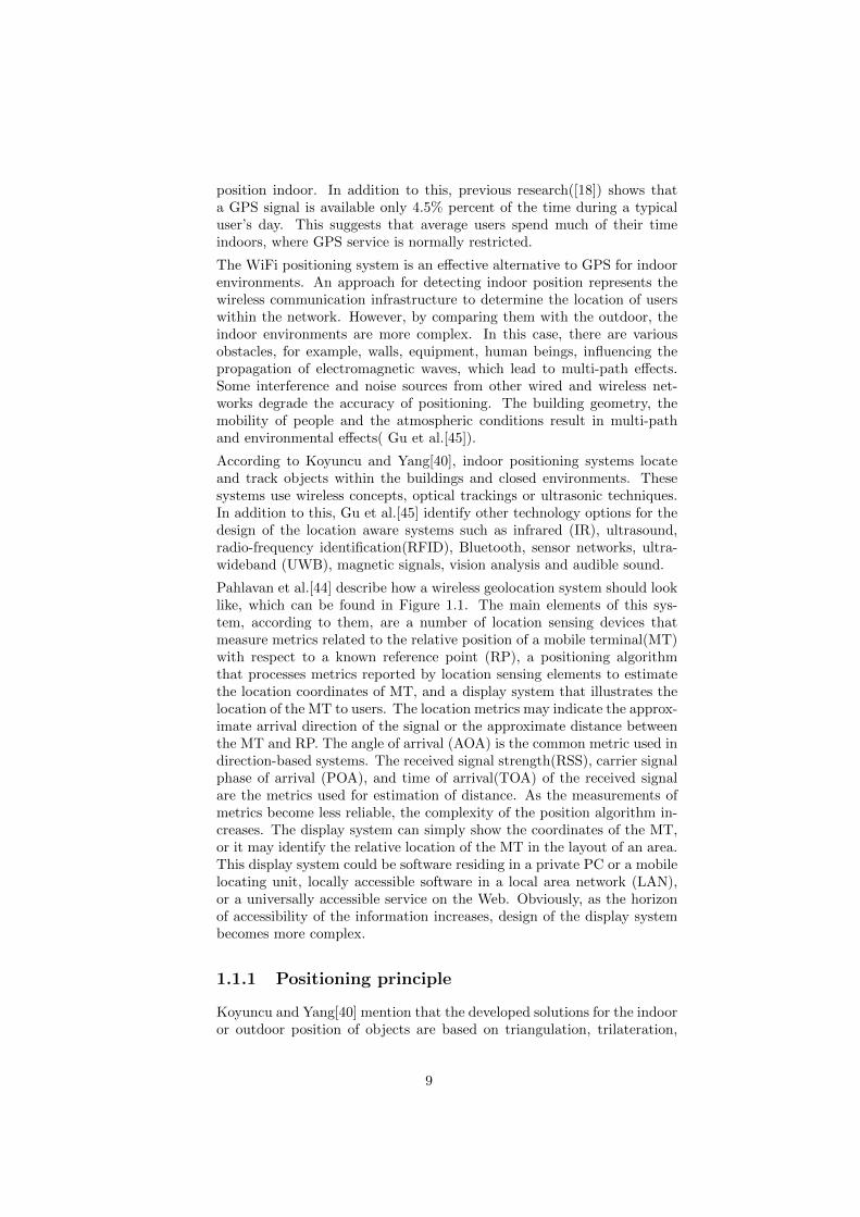
Pahlavan et al.[44] describe how a wireless geolocation system should looklike, which can be found in Figure 1.1. The main elements of this sys-tem, according to them, are a number of location sensing devices thatmeasure metrics related to the relative position of a mobile terminal(MT)with respect to a known reference point (RP), a positioning algorithmthat processes metrics reported by location sensing elements to estimatethe location coordinates of MT, and a display system that illustrates thelocation of the MT to users. The location metrics may indicate the approx-imate arrival direction of the signal or the approximate distance betweenthe MT and RP. The angle of arrival (AOA) is the common metric used indirection-based systems. The received signal strength(RSS), carrier signalphase of arrival (POA), and time of arrival(TOA) of the received signalare the metrics used for estimation of distance. As the measurements ofmetrics become less reliable, the complexity of the position algorithm in-creases. The display system can simply show the coordinates of the MT,or it may identify the relative location of the MT in the layout of an area.This display system could be software residing in a private PC or a mobilelocating unit, locally accessible software in a local area network (LAN),or a universally accessible service on the Web. Obviously, as the horizonof accessibility of the information increases, design of the display systembecomes more complex.

1.1.1 Positioning principle

Koyuncu and Yang[40] mention that the developed solutions for the indooror outdoor position of objects are based on triangulation, trilateration,

9

Figure 1.1: The diagram of a wireless geolocation system, according to Pahlavanet al.[44]

and multi-lateration methods using light[42], ultrasound, or radio signals,which provide positional information. However, Nuaimi and Kamel[12] ar-gue that the main positioning techniques are: triangulation, scene analysisand proximity, and trilateration, which will be briefly described.

Triangulation is the process of determining the location of a point bymeasuring angles to it from known points at either end of a fixed baseline,rather than measuring distances to the point directly(trilateration). Thepoint can then be fixed as the third point of a triangle with one known sideand two known angles. According to Thomas and Ros[36], triangulation isa common operation not only in robot localization, but also in kinematics,aeronautics, crystallography, and computer graphics.

Scene analysis is another principle of positioning in which fingerprintis used(Nuaimi and Kamel[12]). The authors define a fingerprint as theunique characteristic or collection of characteristics of the scene, whichworks by collecting information from the scene and compare it with theexisting database match for each scene.

Proximity principle is mainly used in Radio Frequency based systems,where a grid of antennas with fixed locations within the building are used.When a person carrying a mobile device is detected, the closest antennarepresents the one taken into consideration when the objects’ location iscalculated. If more than one antenna detects the same mobile device, thenthe antenna that receives the strongest signal is used when determiningthe object’s location(Nuaimi and Kamel[12]).

The main measuring technique used for the determination of coordinatesin this thesis represents trilateration, which is a method to determinethe position of an object based on simultaneous range measurements fromthree stations located at known sites(Thomas and Ros[36]).

In two-dimensional geometry, it is known that if a point lies on two circles,then the circle centers and the two radii provide sufficient information to

10

narrow the possible locations down to two. Additional information maynarrow the possibilities down to one unique location[37].

In three-dimensional geometry, when it is known that a point lies on thesurfaces of three spheres, then the centers of the three spheres along withtheir radii provide sufficient information to narrow the possible locationsdown to no more than two (unless the centers lie on a straight line). Amethod for determining the intersections of three sphere surfaces given thecenters and radii of the three spheres is described and the entire derivationcan be found in the appendix chapter based on the information explainedin[37].

1.1.2 Applications

Sayed et al.[43] identified the main applications of location based systems.According to these authors, the forecasted business potential of these sys-tems is tremendous world-wide as the number of users that own a cell-phone increases. Thus, they believe that the most important applicationsare the following:

– Emergency services, because a high percentage of calls to theseservices represent calls made by using a cell-phone.

– Mobile advertising, as mentioned before it can be used for trackingand attracting customers.

– Asset tracking, as it can be used for security services for locatinga lost child, patient, pets, or assets.

– Fleet management, because it can help police forces identify cars,taxi companies, etc.

– Location-based wireless access security for avoiding the inter-ception of digital information.

– Location sensitive billing which uses the location information ofwireless users to offer variable-rate call plans or services based on thecaller location.

– Indoor navigation for identifying places of interest

Pahlavan et al.[44] mention another important application in the publicsafety and military applications, where indoor geolocation systems maybe important for tracking inmates in prisons, navigating policemen, firefighters, and soldiers who need to complete their missions inside buildings.In addition to this, Gu et al.[45] write about various other scenarios suchas fitness case and conference scenarios.

Zeimpekis et al.[13] affirm that the wireless tracking systems promise toenable the development of advanced mobile location systems in both thebusiness-to-consumer(B2C) and business to business markets. The au-thors state that wireless positioning techniques have attracted much in-terest and research recently since they represent a core enabling technologyfor a continuously increasing number of mobile business applications.

11

1.2 Security and privacy requirements

The security of a system is the extent of protection against some unwantedoccurrence such as the invasion of privacy, theft, and the corruption of in-formation or physical damage. The quality or state of being protectedfrom unauthorized access or uncontrolled losses or effects should be givento potential LAS clients. Safety is a property of a device or process whichlimits the risk of accident below some specified acceptable level. In addi-tion, several aspects of privacy, such as approval by the user need to beconsidered[34].

The level of privacy influences the approval by the user:

1. How comfortable are users with their data (e.g., trajectory) beingstored by another party?

2. Do users have legal concerns about their privacy?

3. If so, can private users be motivated to provide personal data?

Approval also includes the requirements for the system to allow certifica-tion by authorities, e.g., if there is a need for admissibility in court, therequirements for the system to deliver evidence should be given. Insurancecompanies should point out their policies concerning approval.

Kapadia et al. [23] study intensively the security challenges that arise fromthe location detection of the devices. The authors propose the followingmethodology with respect to the security challenges such as privacy, in-tegrity, and availability, which should be individually tackled. In additionto this, Harris et al.[25] propose three basic privacy groups in which aparticipant can have one of the following profiles:

– fundamentalist - people that have very high privacy concern

– pragmatism - people that belong to a middle group with balancedprivacy attitudes

– unconcerned - people that have little to no concern about con-sumer privacy issues

According to Mautz[34], the data privacy issue can be tackled from theperspective that users will want to control who may access to the informa-tion about themselves. Consolvo et al.[24] believe that the most importantfactors for participants to share their location are the following:

– who requests the information?

– why does this person request this information?

– what will be useful to this person?

Other important factors that influence whether participants want to dis-close information of their location, which may not be important for thisanalysis, but play a key role in social media represent activity & mood.According to Consolvo et al.[24], participants were more willing to disclose

12

their location when they were “depressed” and they disclosed least whenthey were “angry”.

On one hand, in the same study, 56% of the participants were concernedwith the privacy and security linkage of information from the location-enhanced applications for social relations. In addition to this, some of theparticipants were worried of a third party or unintended individual spyingon their information or getting hold of their actual device.

On the other hand, Sadeh et al.[26] prove that people tend to be con-servative about disclosures at first, but tend to relax their policies overtime as they become more comfortable with mobile applications, in theircase called Peoplefinder, and with how others are using it to find theirlocation. In the end, the authors state that “this finding suggests thatsystems should help people stay in their comfort zones while also helpingthem evolve their policies over time”.

Even though the literature states that over time people stop being con-cerned of the privacy issues, the press does not support that. Forbes[28],one of the most important business newspapers, presented the story ofa coffee shop which had to stop using the WiFi location aware systems,due to the privacy concern of its customers even though the tracking wastransparent and there was also an opt-out feature built.

1.3 Projects in the literature

The literature is rich in articles that include projects related to locationaware systems. However, these systems are small, pilot projects thatrecord and analyze data for a small amount of time and these projectscan be compared with the KPMG LAS system which is built to provideuseful location-based insight for both users and clients.

Chon et al.[8] implemented a system called ”LifeMap” which represents asmart-phone-based context provider and a cost-efficient technology usedfor collecting indoor user context data. LifeMap uses inertial sensors inthe smartphone to provide indoor location information. The informationis combined with GPS and WiFi positioning systems to generate usercontext in daily life. The authors emphasize that there is need for suchsystems in order to improve the quality of services. The authors use asexample finding the locations of a store most frequently visited.

Rekimoto et al.[5] developed a personal location-logging system called“LifeTag” that is based on the PlaceEngine location platform. The userof this system carries a small WiFi sensing device that periodically recordssurrounding WiFi fingerprint information (WiFi access point IDs and re-ceived signal strength). Later, this recorded information is convertedinto actual location logs by accessing the PlaceEngine’s WiFi locationdatabase.

Another interesting study was performed by Jiang et al.[7] who designeda remote pest monitoring system based on wireless communication tech-nology. This system automatically reports environmental conditions and

13

traps pest in real-time. The acquired data was integrated into a databasefor census and further analysis.

Another interesting project is AnonySense, a privacy-aware architecturedeveloped by Cornelius et al[22] for realizing pervasive applications basedon collaborative, opportunistic sensing by personal mobile devices. Ap-plications are allowed by AnonySense to submit sensing tasks that willbe distributed across anonymous participating mobile devices. Later sen-sor data reports are received back from the field that are verified andanonymous. Their prototype is evaluated through experiments and twoapplications(a WiFi rogue access point and a lost-object finder).

1.4 Market research

There is an entire industry of location aware systems focused on WiFitracking. Several companies have been identified as main players in themarket. These companies will be briefly described based on the servicesthey promise to offer, their target and main clients, and other interestingaspects that were available on the internet. The positioning techniquesthat the companies use are not disclosed.

A lead developer of such technologies represents Euclid Analytics[29].Their office is located in San Francisco. According to their website, theytranslate anonymous device data into customer intelligence. Euclid looksat the visitor behavior based on WiFi data, shopping patterns of customerdata, and calculates performance metrics. They target several industries,such as: executive, marketing, operations, IT. In addition to this, theyoffer calculations related to the most important KPIs: storefront conver-sion, average shop time, engagement rate, bounce rate, loyality, sales perday, conversion rate, sales transactions, average sales per week, outsideopportunity, window performance, shopper engagement, store hours op-timization, cross-shopping. On their website, they do not disclose anyinformation related to their clients.

Another competitor represents PurpleWiFi, which targets its services tothe following sectors: retail and leisure, hospitality, health and educa-tion, travel an transport, telecoms, marketing, public sector and commer-cial, and, lastly, but not the least, the event management. The com-pany is located in Manchester, UK. According to its website[30], thereare several business case studies where the company implemented theWiFi tracking and statistics: the Caesar Entertainment UK(casino in-dustry), Orchards Shopping center(in West Sussex, UK), the CanterburyCathedral(visitors tracking), Alhambra shopping center, Crystal Ski Holi-days(implementation of WiFi tracking for ski resorts in France, Italy, andAustria), etc.

RetailNext is another in-store analytics company which combines the datafrom various sources such as: WiFi & Bluetooth devices, video cameras,point of sales data, staffing systems, weather, promotional calendars, pay-ment cards and offers a web dashboard with custom reports combined withmobile apps based on which predictive analytics can be done. According

14

to their website[31], their customers are the following: Bloomingdales,Pepsico, Americal Apparel, P&G, and various other shops. The companystarted in 2007 with their headquarters in San Jose, California, but it alsohas a Dutch partner called WiFiProfs that offers the same services. Thecompany has received last year many awards for being one of the mostinnovative companies.

Another Dutch group that offers a mixture between analytics and track-ing technologies represents the Moreless group. Bluetrace is one of thecompanies that belong to the Moreless group umbrella that offers WiFitracking solutions, which started in 2005. The company targets compa-nies, public institutions, and governments and they offer a platform forcustomer loyalty and online marketing combined with tracking data. Themain clients of Bluetrace are: Citroen, Bas Group, Febo, Seidensticker,Galleria Boromea, Ryanair, municipality of Haarlem etc. This companywas in the news for not appropriately handling data privacy, they did notinform the visitors of the store that they were being tracked[56].

Polestar[27] represents a French company which offers indoor/outdoor po-sitioning solutions with offices both in Toulouse, France and Palo Alto, US.The company was founded in 2002. Their technology is a mix betweenGPS, WiFi, Bluetooth Low Energy, and motion sensors that adopt todifferent environments and existing networks. In addition to this, theydeveloped the NAO campus mobile application for improving the locationbased services. Their market solutions are split in four main categories:shopping malls& large retailers, transportation, museum and theme parks,and convention centers. For the large shopping malls, they offer both themobile application for the customers, which can use the NAO Campusmobile app for finding out where their favorite shops are located, and thetools for extracting information about customer patterns, paths, and dwelltime for the retailers. In the transportation area, their client is the ParisCharles de Gaulle Airport for which they used the same type of mobileapplication. They also work with two internationally renowned museumsdevoted to the promotion of science and technology and based in Paris,La Cite de la Sciences and La Palais de la Decouverte.

Another European company that offers indoor location analytics is theGerman company Infsoft[32]. This is performed by combining multiplemobile sensors, such as: GSM, 3G/4G(LTE), WiFi, magnetic fields, com-pass, air pressure, barometer, accelerometer, gyroscope, Bluetooth andGPS and they promise an accuracy of 1meter. In addition to this, thecompany offers interactive 2D and 3D maps.

15

Chapter 2

Comparison between thetwo developed algorithms

2.1 Description of the algorithms

Two algorithms were developed by KPMG for determining the locationof devices based on WiFi radio signals. The two algorithms use differentmethods to determine the location of the packet source. In this chap-ter, the algorithms will be briefly described below and their performancewill be compared from multiple perspectives: the resolution of calculatedcoordinates, the number of detected mobile devices, etc.

The algorithms are called the Fitter and the Trilaturator. Both take asinput the same information: the source MAC address(sourceMAC), theid string of the routers(drone id), the raw WiFi signals that have beencaptured(signal strength), and the time of the measurement(measurementT imestamp).The dataset that contains all this information will denoted for simplicitythe raw dataset. This information is recorded by the routers which com-municate with the mobile devices and send the input information for thealgorithms to the Kismet server. The entire process can be visualized infigure2.1. Then, the information is stored on the storm cluster using SSH.The algorithms run on the Storm cluster, which sends the output(e.g.sourceMAC, timestamp, and coordinates, Section 2.1.3) to MongoDB forstoring.

16

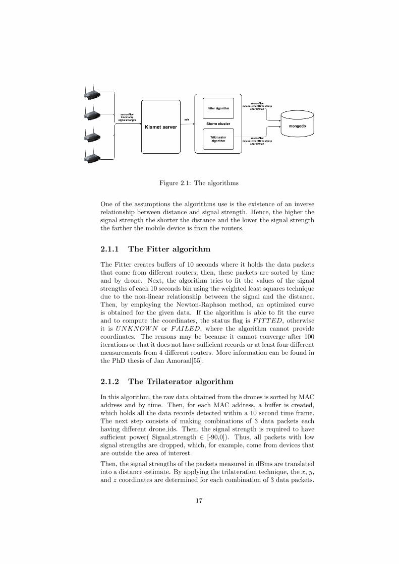
Figure 2.1: The algorithms

One of the assumptions the algorithms use is the existence of an inverserelationship between distance and signal strength. Hence, the higher thesignal strength the shorter the distance and the lower the signal strengththe farther the mobile device is from the routers.

2.1.1 The Fitter algorithm

The Fitter creates buffers of 10 seconds where it holds the data packetsthat come from different routers, then, these packets are sorted by timeand by drone. Next, the algorithm tries to fit the values of the signalstrengths of each 10 seconds bin using the weighted least squares techniquedue to the non-linear relationship between the signal and the distance.Then, by employing the Newton-Raphson method, an optimized curveis obtained for the given data. If the algorithm is able to fit the curveand to compute the coordinates, the status flag is FITTED, otherwiseit is UNKNOWN or FAILED, where the algorithm cannot providecoordinates. The reasons may be because it cannot converge after 100iterations or that it does not have sufficient records or at least four differentmeasurements from 4 different routers. More information can be found inthe PhD thesis of Jan Amoraal[55].

2.1.2 The Trilaterator algorithm

In this algorithm, the raw data obtained from the drones is sorted by MACaddress and by time. Then, for each MAC address, a buffer is created,which holds all the data records detected within a 10 second time frame.The next step consists of making combinations of 3 data packets eachhaving different drone ids. Then, the signal strength is required to havesufficient power( Signal strength ∈ [-90,0]). Thus, all packets with lowsignal strengths are dropped, which, for example, come from devices thatare outside the area of interest.

Then, the signal strengths of the packets measured in dBms are translatedinto a distance estimate. By applying the trilateration technique, the x, y,and z coordinates are determined for each combination of 3 data packets.

17

If the number of combinations reaches 1.000(this threshold is introducedto reduce the computation time), the algorithm stops and computes theaverage values of the x, y, and z coordinates. Besides these values, theuncertainties of both x and y coordinates are also calculated and are equalto the standard deviation of all the computed combinations. These valueswill represent a record in the dataset that is being used for the analysis.

2.1.3 Dataset format of the algorithms

The datasets that we will do the analysis are the result of the trilaterationprocess, which contain the following fields:

– measurementTimestamp - represents the date and time when themeasurement was performed

– sourceMac - represents the hashed MAC address of a device

– coordinates - the calculated coordinates

∗ x - represents the calculated x coordinate by the algorithm

∗ y - represents the calculated y coordinate by the algorithm

– error - the error of the algorithms(the standard deviation of thealgorithms)

∗ errorx - is the calculated error for the x coordinate of the algorithm(σx)

∗ errory - is the calculated error for the y coordinate of the algorithm(σy)

In addition to this, a new variable was introduced to the dataset which iscalled ∆time. The ∆time represents the difference between two consecu-tive timestamps tij of a hashed MAC addresses.

∆timeij = tij − ti(j−1),

where i corresponds to a certain MAC address and the j represents theindex of the interval time of the detection. In addition to this, the firstdetection of a hashed MAC addresses is always initialized with 0. Thisvariable is useful, because it can give us an indication of how long it takesbetween two consecutive detections of the same MAC address. The ∆timeis calculated in minutes and the reason why this measurement unit waschosen was because it was easier to work with it.

Another two variables are introduced which are the residuals for the xand y coordinates. The residuals can only be calculated, if the actualcoordinates are known, by using the following relationships:

residualx = x− x

residualy = y − y

where x and y represent the actual value of the coordinates, which cancome from actual measurements or test cases, while the x and y representthe determined coordinates.

18

2.2 Comparison between the performance ofthe algorithms

The performance of the algorithms will be evaluated on the dataset fromthe CHEP conference by looking at the resolution for the x and y coor-dinates and the number of detected devices, which both depend on thedevice type as well as the time of the day. Therefore, an analysis will beperformed by looking at how different types of devices behave, what is theresolution of the x and y coordinates, as well as the impact that the timeof the day may have on the number of detected devices.

2.2.1 The resolution

The analysis of the resolution is based on the raw CHEP data. The logscontain an experiment where an iPad device was at a fixed position(x =33.2m and y = 18.6m) for an hour and half. This experiment gives anindication of how often this device could ideally be detected if it was notmoved and what the accuracy of the determined positions is comparedto the known position. Moreover, we can discover whether the actualcoordinates can be used for further analysis.

The resolution analysis is performed by comparing two different histograms:the residuals versus the errors of the algorithms for both x and y coordi-nates and the pull distributions for both coordinates.

The residuals versus the errors of the algorithms

The histogram of the residuals versus the uncertainties of the algorithmsof each of the coordinates gives information about how large the measure-ment errors are and whether there is a bias. The residuals were obtainedby taking the difference between the coordinates calculated by the algo-rithms and the actual coordinates of the iPad device. In this sense, bothalgorithms will be compared by looking at their average x and y coordi-nates and the shapes of their residuals’ versus errors’ distributions.

On one hand, as it can be seen in the case of the x and y coordinatesof the Fitter algorithm(Figure 2.2a and Figure 2.3a), the distributions ofthe residuals follow a standard normal distribution slightly shifted to theleft side and slightly shifted to the right side, respectively. The mean isnot centered around zero, as expected. For the x coordinate, it has anapproximate value of −1m, while for the y coordinate, it has an approx-imate value of 1m. Thus, both means are biased. When looking at theuncertainties of the coordinates, it can be observed that the uncertaintieson the coordinates are approximately ±5m for both x and y.

On the other hand, the distribution of the x coordinate in the case ofthe Trilaterator algorithm does not follow the normal distribution(Figure2.2b and Figure 2.3b). However, the distribution of the residuals for they coordinate has the shape of a Gaussian distribution.

19

For further insight about the measurement errors, these plots should beinterpreted together with the second plot of the Pull distribution, whichgives much more information about the measurement errors.

(a) Fitter algorithm

(b) Trilaterator algorithm

Figure 2.2: The residuals versus the error of both algorithms for the x coordinate

20



Figure 2.3: The residuals versus the error of both algorithms for the y coordinate

The Pull distribution of the x or y coordinate

Another method for analyzing the resolution of the calculated coordinatesrepresents the pull distribution, which has the following formula:

pullx(i) =(xi − actualx(i))

σx(i)

pully(i) =(yi − actualy(i))

σy(i)

21

where the xi and yi represent the determined coordinates, the actualx(i)and actualy(i) are the actual measurements of a MAC address, and theσx(i) and σy(i) are the errors of the algorithms.

In Figures 2.4a and 2.4b and 2.5a and 2.5b, the Pull distributions of theboth x and y coordinates are shown. The width of the Pull distributionsgives more information about the measurement error. In the case of theFitter algorithm, the center of the distribution for the x coordinate liesaround −1m. Normally, this distribution should be centered around 0,however in this case it can be observed that the entire distribution isshifted to left which means that the mean is biased.

In the case of the y coordinate, the Fitter algorithms also has its mean notcentered at 0m, but shifted to the right side with a value of approximately1m. However, the Trilaterator algorithm has its mean centered around 0m.

In the end, almost all three mentioned distributions resemble the stan-dard normal distribution, except for the Trilaterator distribution of the xcoordinate.

22



Figure 2.4: The Pull distribution of x coordinate of both algorithms

23



Figure 2.5: The Pull distribution of y coordinate of both algorithms

The animation of the reconstructed coordinates path in time

The animation of the reconstructed coordinates path in time is useful forlooking at the path a device follows. This is performed from one detectionto another. The plots from Figures 2.6a and 2.6b represent the positionsof the detected coordinates of the iPad experiment, where this device wasplaced for one hour and a half without being moved. The labels of thepoints represent the values between two consecutive detections(∆time).The initial value of the ∆time is 0 seconds.

It can be seen that the values of the Fitter algorithm are centered around

24

the actual point, which had the coordinates x = 33.2m and y = 18.6m.However, it can be seen that there are also some points which deviate farfrom the values of the actual coordinates. A similar situation occurs alsowhen using the Trilaterator algorithm. By comparing the performance ofthis algorithm with the one of the Trilaterator, it can seen that the pointsare better centered than the ones calculated by the latter, which has alarger spread around the centers of interest. This corresponds with theobservations made with the residuals and Pull distributions. Thus, theFitter algorithm behaves better than the Trilaterator algorithm.

Another interesting aspect may be the number of points that were recordedfor the iPad devices, which can be seen in Table 2.1. The Fitter algorithmhas detected more points for the iPad device than the Trilaterator algo-rithm which has 212 points, 32 fewer points than the first algorithm. Inaddition to this, the average value of the coordinate x is 30.7m in thecase of the Fitter algorithm, which has a much higher value than the Tri-laterator algorithm with x = 26.8m. However, the actual value of the xcoordinate was x = 33.2. This means that for this coordinate the Fit-ter algorithm performed better than the Trilaterator, but still with somedeviation from the actual value.

In addition to this, the same situation can be seen for the y coordinate forthe Trilaterator algorithm which has the average value of the y coordinateequal to 15.4m, which is less than the Fitter algorithm with an averagevalue of the y = 18.3m coordinate close to the actual value of the ycoordinate y = 18.6m.

The root mean squared error will also be used for the comparison betweenthe two algorithms, which constitutes a measure of the differences betweenvalues predicted by a model or an estimator and the values actually ob-served. According to Wikipedia[41], the RMSE represents a good measureof the accuracy, but which can used only to compare errors of differentmodels for a particular variable.

On one hand, the results for the x coordinate show that on average the de-viation from the actual value is 7.8m for the Fitter algorithm, which is lessthan the RMSE obtained by using the Trilaterator algorithm, which hasa RMSE of 9.8m. On the other hand, in the case of the y coordinate theresults show that the Trilaterator performs better than the Fitter with aRMSE of 5.7m compared to 6.4m. As it can be seen, the calculated coordi-nates of both algorithms seem to be less and seem to have deviations fromthe actual coordinates. A possible explanation may be that the calculatedcoordinates are not reliable and that the models need improvement andmuch more testing. The large root mean squared error can be explainedby the possibility that the actual coordinates were not very well recordedin the logs.

25

Element Fitter algorithm Trilaterator algorithm

The number of points 244 212Averagex(m) 30.7 26.8Averagey(m) 18.3 15.5RMSEx(m) 7.8 9.8RMSEy(m) 6.4 5.7

Table 2.1: Statistics



Figure 2.6: The animation of the detected coordinates of the iPad

26

2.2.2 Device dependency

In this section, two different devices are analyzed with respect to twodifferent quantities: the number of detections, but also how long it takesbetween two consecutive detections. These devices were recorded as testsduring the CHEP conference. One of these devices was the iPad, whilethe other one represented a cell-phone which did a lot of streaming. Theintention was to check whether the cell-phones behave differently.

By looking at plots of the iPad of both algorithms in Figures 2.8a and2.8b, it can be observed that in most of the cases the device is beingrecorded quite often in time intervals less than one minute. However, inboth pictures, it can be seen that there exists a large time gap betweenapproximately 13 : 20 and 13 : 30, were the detections took more thantwo minutes with a maximum less than 10minutes. Because it is knownthat the iPad was not moved, it cannot be inferred that the device actuallyswitched off. This situation can be either a technical problem or it may bedue to an insufficient number of points based on which the trilaterationtechnique can be applied and, thus, the algorithm could not provide asolution.

27



Figure 2.7: The delta time(’time differences’) and detections with respect to themoment in time and algorithm

28



Figure 2.8: The delta time(’time differences’) and detections with respect to themoment in time and algorithm

In the case of the second device, which represents a cell-phone with stream-ing data that was constantly moving, the time of the recording for thisdevice was spread over an entire day and the detections can be observedstarting from 07 : 00 until 17 : 00.

According to Figure 2.8b, the Trilaterator algorithm was able to calculatemany more points with coordinates. For example, in total the Fitteralgorithm has 1.098 records but only for 275 records the fitted coordinateswere provided(the percentage of the fitted coordinates is approximately25%). However, the Trilaterator algorithm was able to fit the coordinates

29

for 901 records. In the end, a positive aspect that can be drawn from bothplots is that they have the same shape, even though the number of fittedpoints is very different from each other.

Another interesting aspect can be seen that starting from 13 : 00 o’clock,there is a very large gap of 45 minutes for the Fitter algorithm, while forthe Trilaterator algorithm it was only of approximately 33 minutes. It canbe the case that the Fitter algorithm did not have enough information toactually calculate the coordinates for that particular detection. Anotherpotential explanation for this large time gap between detections may bethat the device may have moved away from the area where the locationaware system was installed which is in accordance with the logs of thecompany for this specific device.

Due to the absence of reference points, the resolution of these detectionscannot be determined. Moreover, it is not possible to determine whetherthe actual information provided by the coordinates extracted from thealgorithms is relevant and can be used. This issue is tackled Chapter 4and Chapter 3, where controlled experiments are performed.

2.2.3 Number of devices in time

In this subsection, we will analyze how the algorithms perform on anaggregated level and how many devices are actually recorded during thetime of the day if this behavior is spread around on a day level between07 : 00 until 21 : 00. It provides information related to the numberof devices that are recorded during this period within a time interval of5 minutes. This means that each value contains the number of uniquedevices seen every 5 minutes.

First of all, the figures of plots 2.9a and 2.9b have consistent shapes.It seems that the Fitter algorithm has detected more devices than theTrilaterator algorithm. In this plot(Figure 2.9a), there was no cut madesuch that, for example, devices which are detected less than 3 times areavoided. This means that all the seen devices are taken into consideration.

As it can be seen in the Figures 2.9a and 2.9b, there are four different peaksin the data, followed by dramatic decreases. These peaks and decreaseslast around one hour each and have almost the same number of detecteddevices.

Based on the schedule of the conference, the first peak corresponds to adramatic increase which can be explained as the number of people arrivingat the conference. The start time of the conference was 09 : 00. Thedecrease after the first peak corresponds to the fact that people stoppedusing their cell-phones or devices. Thus, this may mean that they attendedthe conferences and their devices became idle or they were turned off orthey just left the area where the location systems were installed.

The second peak may be explained by the fact that after attending theconferences, people started checking their devices more often or streamingdata. This increased activity produced thus more data. In addition to this,it may also indicate a coffee break taken after the first set of presentations.

30

The third peak corresponds to the lunch time, where people also come tothe area which was recorded by the location aware systems. In additionto this, the third decrease may mean people attending presentations orpeople that are actually leaving the conference. An interesting aspect isthat the number of detected devices during the first three peaks does notchange significantly, which denotes that once people arrive their numberdoes not actually change or if it does it is not significant.

The last peak does not have the same number of devices as the previousthree. As mentioned before, there can be the situation that people left theconference and did not come back anymore. However, not all of them leftyet. After this last peak, one can see a dramatic decrease of the numberof detected devices which corresponds to the number of people leaving theconference for good.

31



Figure 2.9: The number of detected devices during a day for both algorithms

2.2.4 Histograms of the time difference between de-tections

As previously mentioned, the ∆time represents a measurement for thetime difference between two consecutive detections. In Figures 2.10a and2.10b, the histograms of the ∆time can be visualized. In the case ofboth algorithms, the devices communicate in less than two minutes. Aninteresting difference that we can see between the two of them is that thereseem to be more devices that have the delta time higher than 5 minutesin the case of the Fitter algorithm than for the Trilaterator algorithm. Apotential explanation can be that the Trilaterator algorithm sometimes

32

calculates more data points than the Fitter algorithm, because the latteralgorithm needs much more information. Hence, it has a smaller ∆time.

The value of the ∆time = 5 will be the threshold for the next chapter,where we will try to differentiate the devices that either are present(∆time <5 minutes) or have left(∆time ≥ 5 minutes), even though they are presentin the area with the mounted devices. This information will be also usedfor the controlled experiments, as it is important to understand in whichsituation we may draw the conclusion that a device is gone or missing.



Figure 2.10: The histogram of the delta time between for both algorithms

33

2.2.5 Number of detections per device

Ideally, a device can be detected every 10 seconds within the time intervalbetween the moment it appears and disappears from the area where thelocation aware system is installed. However, this is not actually achieveddue to the unknown state of the device which can either be idle or switchedoff, etc. In addition to this, the location aware systems record also deviceswhich are close to the area under detection or devices of people walkingoutside. These devices usually have less than 5 detections with a verylarge ∆time between two consecutive detections.

What we would like to find is a potential threshold with respect to thenumber of records a device should have such that the dataset is cleanedof unwanted data. After several selected values of the threshold, the valuewhich stood out was 5 records as it was the cut-off of the histogram withthe number of detections per device. In order to increase visibility ofthe number of detections, we decided to split that histogram into twoparts: less than 5 records and more than 5 records. In Figures 2.11a,2.11b, 2.12a, and 2.12b, it can be observed that the histograms of thetwo algorithms look similar for both less and more than 5 records. Thisconstitutes an interesting result as this seemed unexpected given the otherdiscovered differences between the algorithms, such as: number of detecteddevices and the different number of detections per device(iPad animation).Moreover, the highest number of records for a device can be seen for MACaddresses which are detected only once. These MAC addresses should beeliminated.

34



Figure 2.11: The histograms of the detected devices with less than 5 records forboth algorithms

35



Figure 2.12: The histograms of the detected devices with more than 5 recordsfor both algorithms

2.3 Conclusion

In this chapter, we performed the comparison between the Fitter andTrilaterator algorithms. The two have similar performance with re-spect to their resolution and efficiency. Nevertheless, the Fitter performsslightly better from a resolution perspective and, therefore, the rest ofthe analyses and models will be performed on the datasets obtained byapplying the Fitter algorithm.

36

Chapter 3

Modeling the timedependency of detectingWiFi devices

In this chapter, we propose two models that calculate the probability ofdetecting a mobile device over time based on the Fitter dataset obtainedfrom the CHEP conference. These two models are called the Basic modeland the Cut-off model. The cut-off model uses the same principle of thebasic model, but makes two additional assumptions:

– If somebody is not detected for more than 5 minutes, then that personleft the area of analysis.

– A mobile device should have at least 5 detections.

These two thresholds of 5 minutes and records, respectively, were selectedbased on the results of Chapter 2 from the histogram of the delta timeand the histograms of the detected devices.

The models also represent an attempt to identify in which state a deviceis during a time interval ∆time. It is a challenge to determine in whichstate a device is, because the data recorded at the CHEP conference doesnot contain information on the state of the WiFi devices. The state of amobile device may be: “active”(it communicates with the routers and it isin the area of the analysis), “gone”(left the area of analysis), “missing”(inthe area of analysis, but not detected because of technical issues or thedevice is idle/switched off).

3.1 Basic model

Let there be a time period within the interval [timestart, timestop] whichcan be either a day, half a day, or any other desired interval time. Bothtimestart and timestop have the following structure: “yyyy-mm-dd HH:MM:SS”,

37

where y stands for year, m for month, d is for day, H for hour, M forminute, S for second.

The time interval represents the time interval for which we zoom-intothe selected period ([timestart , timestop ]). The time interval is expressedeither on a second or minute level. In this section, we zoom-into the[timestart, timestop] on a 5 minute level, because we would like to get afirst impression regarding the CHEP data.

Let an Arrival represent the first time a WiFi device MAC address isdetected within a selected period of time. This means that before thisdetection there was no previous information related to this MAC address.A Departure is defined as the last time a MAC address is detected. Hence,one cannot find any later record in the database besides this one and wesay that “it has left the system”.

Figure 3.1 illustrates the times of arrival and departure within a timeperiod [timestart, timestop]. This pattern is similar for most WiFi devices.An exception constitutes the MAC addresses with a single record whichhave the time of arrival equal to the time of departure.

Figure 3.1: The diagram with the time of arrival, departure within a time period

A “Missing” MAC address represents a MAC address which has anArrival,but it does not have a Departure. However, this MAC address is not be-ing detected within certain time intervals. This situation can occur, dueto several reasons: the drones do not function, the drones are busy, thedevice is not in the area of detection, or the device is idle.

Two arrays are defined with the size equal to the number of unique MACaddresses extracted from the dataset, Arr and Dep. For each MAC ad-dress i ∈ [0, n − 1], where n represents the number of unique MAC ad-dresses, we compute the interval time between its arrival(Arri) and itsdeparture(Depi) within the selected time period.

Arri = time arrivali ∈ [t, t+ time interval]

Depi = time departurei ∈ [t, t+ time interval]

where t ∈ [timestart, timestop] and time interval represents the user se-lected time interval for which the analysis is made(e.g., 10 seconds, 5minutes, etc.).

The next step is to introduce the number of arrivals and departures withina time interval denoted asArrivals[t,t+time interval] andDepartures[t,t+time interval].These two quantities can be determined by aggregating and counting the

38

MAC addresses an arrival or departure, respectively within that time in-terval, which is written as follows:

Arrivals[t,t+time interval] =∑

Arri ∈ [t, t+ time interval]

Departures[t,t+time interval] =∑

Depi ∈ [t, t+ time interval]

Besides the Arrivals andDepartures, the total number of unique detecteddevices within [t, t+ time interval] can be computed, which we denote asTotal detected[t,t+time interval]. The following relationship holds:

Total detected[t,t+time interval] = Arrivals[t,t+time interval]+Departures[t,t+time interval]

+Active[t,t+time interval] − In out[t,t+time interval]

where the Active[t,t+time interval] represent the MAC addresses that ar-rived in previous time intervals, but have not departed yet, and they arecurrently detected within the time interval of [t, t + time interval]. TheIn out[t,t+time interval] represents the number of unique MAC addressesthat arrive and depart in the current time interval [t, t + time interval].The reason why we need to correct with the In out[t,t+time interval] is thatwe add these MAC addresses twice: first for their arrival and second fortheir departure, but actually, they represent the same MAC addresses.Hence, they should be taken into consideration only once.

In Figure 3.2, the Arrivals and Departures are plotted together withthe Total detected for the CHEP data on which the Fitter algorithm wasapplied. The time interval was selected to be 5 minutes and the timeperiod is from 07 : 00 until 21 : 00 of the October 15th2013, because wewanted to get a first impression on the CHEP data on a busy day. It canbe observed that the highest number of arrivals are at the beginning ofthe day at 09 : 00 o’clock, before the actual conference starts. Two otherspikes can be seen at around 11 : 00 and 13 : 00. However, for the rest ofthe day, there seems to be a constant behavior of the arrivals.

39

Figure 3.2: The total detections, arrivals, and departures for a 5 minute selectedtime interval from 07 : 00 to 21 : 00

The departures seem to have an opposite behavior, as expected. In thebeginning, the number of departures is small, but different than zero. Thereason is that other devices that pass by or access points are detected bythe routers during the night. At the end of the day, some spikes for thedepartures can be observed which indicate that people leave the confer-ence.

Next, we would like to determine the probability of detecting a device fora time period. Intuitively, the total number of devices(Total detected)seems to be a good choice to be included in the calculation of this prob-ability. However, it does not entirely reflect the correct number of MACaddresses that are present in the system for several reasons: the devicesare in different states, the devices may not be seen by the drones dueto technical problems. Thus, we introduce the ideal number of detectedMAC addresses(Ideal) that represents the number of detected devices ata certain time interval that should be detected by the system. Mathemat-ically, the Ideal can be computed as the difference between the numberof arrivals minus the departures up to time interval [t, t + time interval]as follows:

Ideal[t,t+time interval] =

[t,t+time interval]∑i=[timestart,timestart+time interval]

(Arrivalsi −Departuresi)

40

The probability of detecting a device reflects the portion of detected MACaddresses which arrived in previous time intervals, but which have not leftyet( Active) from the total number of MAC addresses which should haveideally been detected(Ideal). The probability of detecting a device iscomputed as follows:

Pdetected devices[t,t+time interval] =Active[t,t+time interval]

Ideal[t,t+time interval]

whileActive[t,t+time interval] can be calculated based on the Total detectionsformula:

Active[t,t+time interval] = Total detected[t,t+time interval]−Arrivals[t,t+time interval]−Departures[t,t+time interval] + In out[t,t+time interval]

In the next plot(Figure 3.3), the ideal number of detected devices versusthe Active is visualized. As it can be seen, the shown number of activeMAC addresses has a similar shape as the Total detected: it has fourspikes as in Figure 3.2. The Ideal has a cumulative shape like a bell.It can be observed that the decrease of the Ideal also corresponds to adecrease in the number of MAC addresses of the Active. This seems aninteresting result, because it indicates that this decrease corresponds topeople that leave the conference, which can be seen for both Active andIdeal number of MAC addresses.

41

Figure 3.3: The ideal number versus the number of detected devices for a 5minute selected time interval from 07 : 00 to 21 : 00

As mentioned before, the probability of detecting a device within a 5minute time interval is calculated by dividing the Active by the Ideal.The result of this division is shown in Figure 3.4. As it can be seen,the shape of the probability is similar to that of the Total detected andActive macs with approximately four different peaks during the day thatmay indicate a time dependency. On average, this probability seems to bearound 0.25± 0.09.

42

Figure 3.4: The probability of detecting a device within a 5 minute selectedtime interval from 07 : 00 to 21 : 00

In the end, the Basic model represents a first approach for computing theprobability of detecting a device. Its advantages are that it is simple andintuitive. This Basic model uses a 5 minutes time interval to computeall the quantities. This time interval is quite large. Hence, it is quitedifficult to give any explanation regarding the devices that left the area ofanalysis and are expected to come back or that are still in there, but notdetected. A solution to this challenge is to zoom in from a minute level toa second level, because we would like to identify how the Fitter algorithmcomputes coordinates for a MAC address every time interval. Besidesthis, the probability of detection may be underestimated, because the theIdeal is overestimated as no assumption was made regarding the fact thatpeople may have left for some time the area under analysis. Thus, in thenext section, we introduce a new algorithm that we expect to overcomethese mentioned limitations.

3.2 Cut-off model

In this section, we present an alternative model to compute all the definedquantities from the Basic model. As discussed in the Chapter 2, the Fitterand Trilaturator algorithms use a 10 seconds buffer for computing thecoordinates of a mobile device. Thus, the lowest time interval in which

43

we can zoom into the dataset is 10 seconds. Besides this, we will performthe computations also on a 30 and 60 seconds level in order to evaluatethe differences compared to 10 seconds.

A threshold on the number of missing intervals for a MAC address isintroduced in this model, because the Ideal may be overestimated dueto the fact that no assumption was made related to the people that mayhave left for a certain amount of time the area under analysis at the CHEPconference. Thus, we correct the Ideal and this corrected Ideal will bedenoted as Corr Ideal. Moreover, this means that every time a MACaddress is missing more than the threshold number of intervals then weassume that that particular MAC address is gone within that delta timeand we correct this disappearance from the Ideal within that time interval.

Corr Ideal[t,t+time interval] = Ideal[t,t+time interval]−Correction[t,t+time interval]

where Correction represents a correction for the underestimation of thevalue of the detected devices. The corrected probability of detecting amobile device is then:

P corrected[t,t+time interval] =Active[t,t+time interval]

Corr ideal[t,t+time interval]

The behavior of a MAC address represents a compressed way to describehow a MAC address has been or not detected, which contains informationabout the time period expressed as the number of consecutive detected in-tervals followed by the number of consecutive missing intervals between itsarrival and departure. This compressed way of describing a MAC addressis efficient when calculating the statistics for very small time intervals as10, 30, or 60 seconds. The reason is that within a day there are largenumbers of 10 seconds time intervals and unique MAC addresses. It maybe inefficient to go through every time interval for each MAC address.Thus, using the behavior overcomes this challenge.

For example, a behavior of a device can be observed in Figure 3.5, wherewe can see that the interval between [Arrival, Departure] covers 18time intervals. Its Arrival is within the 7th interval(the notation of theinterval starts from 0) and its Departure is within the 24th time intervalof time interval size.

44

Figure 3.5: The behavior of a MAC address within a time period betweentimestart and timestop split into multiple time intervals

Hence, we define the behavior of this MAC address as the collection of cal-culated consecutive and missing intervals between the time of arrival untilthe time of departure. We remind the reader that the number consecu-tive missing intervals(′m′) constitutes the number of consecutive intervalswith no detections of the MAC address under analysis, while the numberof consecutive detection intervals(′d′) suggests the number of consecutiveintervals that have at least one detection within every interval. Hence, forthe device in Figure 3.5, its behavior will be:

Behavior = {′d′ :3,′m′ :2,′ d′ :4,′m′ :3,′ d′ :1,′m′ :3,′ d′ :2}.By construction, this collection always ends with a detection(that of thedeparture). In addition to this, we retain the interval numbers of thearrival and the departure(7th and 24th).

The algorithm behind the cut-off model has two parts:

1. The computation of the behavior of all MAC addresses based on thedataset of the Fitter algorithm

2. The calculation of the main quantities:

(a) The total number of detected devices, the arrivals, and depar-tures for every time interval

(b) The active MAC addresses and the corrected ideal

(c) The corrected probability of detecting a mobile device for everytime interval

The first part deals with computing the behavior of all unique MAC ad-dresses that can be found in the dataset. Thus, for each MAC addressi ∈ [0, n − 1] in the dataset, which has more than 5 detections, the al-gorithm starts from its arrival and computes alternatively the number ofconsecutive time intervals with detections(consecutive)and the number ofconsecutive intervals with missing detections(missing) until the depar-ture.

45

For each detection j of a MAC address i, if the time of that detection iswithin the time interval [t, t + time interval], then the number of detec-tions within [t, t + time interval] is calculated. Otherwise, if the time ofa detection is not within [t, t + time interval], then the number of timeintervals with missing detections are calculated, denoted as missing. Themissing is equal to the difference between the time of the current detec-tion and the lower bound of the current time interval t divided by thetime interval size. In this case, there are two situations:

– If the missing number of time intervals is greater than 1, then itmeans that the next detection is located at missing time intervalsdistance from [t, t + time interval]. If consecutive is greater thanzero, then this number of consecutive intervals with detections isappended into the list of behaviors and the consecutive is initializedwith 1. After the consecutive, the missing is also appended to thelist of behaviors. The current time interval t becomes t+missing×time interval.

– Otherwise, if missing is equal to 1, then the next detection is lo-cated within the next time interval. Thus, if the number of detec-tions within this time interval is greater than 0, then the number ofconsecutive time intervals is incremented. The current time intervalt becomes t+ time interval.

As it can be seen, the algorithm goes only through the time intervalswith detections of MAC address i, which increases the performance of thealgorithm, because the intervals with no detections of that particular MACare avoided. In addition to this, using lists as main data structures makesthe computations faster and easier to deal with. The entire algorithm canbe visualized in Section 1 parts 1 and 2. Besides the matrix of behaviors,the function also returns the list of the location of each analyzed MACaddresses, because their location in the dataset is not clearly determinedand there is no simpler way of actually determining it.

The second part of the algorithm deals with calculating the corrections ofthe Ideal by considering “gone” the MAC addresses that have the ∆time

between two detections greater the threshold. These corrections of theIdeal need to be made for the entire time interval in which the MACaddress is missing, at the exact position where the MAC address is notpresent anymore until it actually comes back. In order to calculate thesecorrections in an efficient way, the following elements are needed:

1. List of all behaviors, which contains the behaviors of all unique MACaddresses in the dataset.

2. List of arrivals, which contains for each MAC address i the numberof time intervals after which its arrival occurs. Its size is equal to thetotal number of unique MAC addresses n.

3. List of departures, which contains for each MAC address i the numberof time intervals after which its departure occurs. Its size is equal tothe total number of unique MAC addresses n.

46

Algorithm 1: The computation of the behavior of all MACaddresses-Part 1

[1] Data: dataset[’mac’,’time’]Input: time interval, threshold records, timestart, timestoplist missing=[];list detected=[];list all=[];list macs=[];list arrivals=[];list departures=[];Calculate index= the array with first positions in the dataset of amac(Arr);Calculate the n unique number mac addresses;for i in n-1 do

if Arr[i+1]- Arr[i] ≥threshold recordsthenlist macs.append(dataset[’mac’][i]);t=round(Arr[i]);list arrivals.append((Arr[i]-timestart).seconds/(time interval));list departure.append((Dep[i]-timestart).seconds/(time interval));missing=0;already=0;consecutive=1;c=0;list all=[];for j in range(index[i], index[i+1]) do

if t ≤ raw data[′time′][j] ≤ (t+ time interval)thenc+=1;

myalg

4. intervals - represents the total number of time intervals of user se-lected size between the timestart and timestop and the formula is:

intervals =(timestart − timestop)

(time interval)

The difference between timestart and timestop is expressed in seconds inPython. If we want to determine the number of intervals expressed inminutes, we divide by 60× time interval.The algorithm performs the following steps. For each MAC address i,the arrival and departure are extracted from their corresponding list. Avariable pos retains the starting position of the consecutive intervals withdetections, which initially is equal to the arrival of that particular MACaddress. In addition to this, the length of the list with the behaviorof MAC address i is calculated. Then the iteration over the list of thebehavior of the MAC address i begins. A new variable k records theposition of a detection as long as we have not reached the position ofa missing interval and the Total detected is updated. Next, if we havenot reached the last position in the list of behavior for a particular MAC

47

Algorithm 2: The computation of the behavior of all MAC addresses-Part2

[1] myalg else if thenmissing=(dataset[’time’][j]-t).seconds/interval;if missing>1 then

if consecutive>0 thenlist all.append((’d’,consecutive));consecutive=1;

endlist all.append((’m’, missing-1));t=t+missing × time interval;c=1;

else if missing==1 thenif c>0 then

consecutive+=1;endt=t+time interval;c=1;

endif consecutive>0 then

list all.append((’d’, consecutive));endlist all states.append(list all);endendreturn list all states, list mac, list arrivals, list departures, list index

address(last ′d′ with the last consecutive intervals with detections), thevariable pos is updated with value of the starting interval of the missingplus the number of missing intervals. The variable pos refers now tothe next number of consecutive intervals(next d in the list of behaviorof a MAC). Then, we check whether that particular number of missingintervals is greater than the threshold given by the analyst. The thresholdis used, because we make an assumption that if someone actually leftthe area where the location aware system is installed for more than thethreshold time intervals, then he or she is gone. Thus, for that particularnumber of missing intervals, the Ideal needs to be corrected, and thiscorrection is made by extracting this person/device from the counting.Next, the count cutoff is updated for every time interval in the rangeof missing and we jump only to the intervals with consecutive detections.Otherwise, in case we reached the last element of the list of behaviorfor that particular MAC address, we do not correct anymore the position,because the last element does not contain any other number of consecutivemissing intervals(′m′). The entire algorithm can be visualized part 3.

48

Algorithm 3: The calculation the total detections and correction

[1] Input: list all, list arrivals, list departures, max distance, thresholdn=size(list all);Total detected=array(max distance);count cutoff=array(max distance);for i in range(n) do

arr=list arrivals[i];dep=list departures[i];pos=arr;m=len(list all[i]);j=0;while (j<m) do

k=pos;while k ≤ (pos+list all[i][j][1]-1) do

Total detected[k]=Total detected[k]+1;k+=1;

endif j < m-1 then

pos=k+list all[i][j+1][1];if list all[i][j+1][1] ≥ threshold then

t=k;while t ≤ (list all[i][j+1][1]+k-1) do

count cutoff[t]+=1;t=t+1;

endj=j+2;

end

else if j==m-1 thenpos=k;j=j+1;

end

endreturn Total detected, count cutoff

49

3.2.1 Results

In this section, the results of the cut-off model for three different usertime intervals of 10, 30, and 60 seconds and their probability of detectionare presented.

As we mentioned in the description of the cut-off algorithm, certain pa-rameters need to be selected for this algorithm such as the threshold ofrecords for a certain MAC address, the threshold of missing intervals, andthe period of time. These decisions were made made based on the resultsfrom Chapter 2, where the comparison between the two algorithm wasdiscussed.

Firstly, the threshold records was set to 5. According to Figures 2.11band 2.12a, it can be observed that there is a dramatic decrease of thenumber of devices with more records than 5. The idea behind selectingthis threshold is that the dataset needs to be cleaned from MAC addresseswhich do not have sufficient detections and may damage the analysis andthe model. In addition to this, this quality cut-off removed all the In outMAC addresses which had the arrival and departure within the same timeinterval. Secondly, based on the results of the histogram of the delta inFigure 2.10a, the decision of selecting the threshold of missing intervals to5 minutes was made. In the case of 10, 30, and 60 seconds time interval,the threshold will be 30, 10, and 5 missing intervals, which all represent5 minutes and which were obtained by dividing 5×60s

time interval . Lastly, theperiod of time was chosen to be October 15th2013 from 07 : 00 to 21 : 00.This period was chosen as a regular day of the conference, which can besplit in 5, 040 intervals of 10 seconds intervals, 1, 680 intervals of 30 secondsintervals, and 840 intervals of 60 seconds intervals, respectively.

The results of the cut-off model can be visualized in Figures 3.6a, 3.7a,and 3.8a. As it can be observed, the plots show the ideal, the corrected,the total detections, and the active. The probability of detection is basedon the corrected probability of detection.

Statistics 10 seconds 30 seconds 60 seconds

Average probability 0.337 0.542 0.713Standard deviation 0.131 0.122 0.109Number intervals 5, 040 1, 680 840Threshold missing 30 10 5

Table 3.1: Statistics

As it can be seen in Table 3.1, the average probability increases as weincrease the size of the time interval. This was expected, because theprobability of having detections in a larger interval is higher than havingdetections in a smaller interval. In addition to this, it can be observedthat the probability of detecting someone has a flatter shape now thanin the basic model(Figure 3.4). However, the variations can still be seenwith respect to the time period. Moreover, the original form of four majorpeaks is still present. This structure with four different peaks becomes less

50

evident if a higher time interval is chosen, for example 30 in Figure 3.7b.In the case of the 60 seconds time interval, the shape of the probabilitybecomes flatter and the structure of the variations is less evident(Figure3.8b). The reason between this change is that with a higher selectedtime interval, the results are more aggregated and fewer computations areperformed with more data.

In the case of the 10 seconds time interval, the average probability is0.337, which means that a device is detected on average 33.7% of thetimes between its time of its arrival and departure, while the standarddeviation is 0.131. The same interpretation can be given for the 30secondand 60 second time interval, which have an average probability of detectionof 0.542 and 0.713, respectively. In the end, the results obtained with thecorrection are better than the results obtained from the basic model, whichhad a value of a 0.25± 0.09.

Another interesting aspect that can be observed in the plots of Figures3.6a, 3.7a, and 3.8a is that the corrected ideal and the active number ofdetected devices have similar shapes across all three plots. The differencebetween them is of binning only. This represents a good result, because itreveals that the results are consistent over time, no matter the selectionof the time interval. In addition to this, it can be observed in the sameplots that for the the active MAC addresses and the total detected MACaddresses seem to overlap with each other, because the number of arrivalsand departures per time interval is too small compared to the total detec-tions and the number of In out MAC addresses is zero due to the 5 recordthreshold.

The plots show that during the day there was a failure in the beginningof the day which lasted more than 5 minutes. There were no detectionsduring that time period and the MAC addresses were corrected. However,the ideal number of MAC addresses was not influenced by this failure, asit depends mainly on arrivals and departures. Due to the fact that thecorrected ideal and the active MAC addresses were both equal to zerowithin that period, the probability was set to be equal to 1. Hence, theseplots bring insight not only on what happens on a day level, but theyalso reveal information regarding possible failures of the WiFi tracking.In order to actually interpret correctly the probability of detecting mobiledevices, one would also need to take into consideration the plots of thecounts over day.

51

(a) The total detections, the ideal, the corrected ideal, and the active MAC addressesper 10 seconds time interval

(b) The probability of detecting a mobile device per 10 time interval

52



53



54

3.3 Conclusions

In this chapter, two models were proposed for calculating the probabil-ity of detecting the mobile devices: the “Basic model” and the “Cut-offmodel”. The basic model represents an intuitive model that calculates theprobability of detecting mobile devices without making any assumptions.The results showed that the probability of detecting a mobile devices isapproximately 0.25± 0.09.

Compared to the basic model, the cut-off model cleans the dataset fromMAC addresses with the number of records less than a specified threshold.It also introduces an assumption that all MAC addresses that have a∆time ≥ 5 minutes are gone and it zooms-into the dataset on a 10, 30, or60 second level instead of 5 minutes as the Basic model.

The results of this model show that the probability of detecting a mo-bile device increases considerably and the higher the time interval is, thehigher the probability of detection is.

55

Chapter 4

Controlled table topexperiments

4.1 Introduction

In this chapter, controlled table top experiments are implemented whichreveal insight in how mobile devices communicate with the routers. Inaddition to this, the Fitter algorithm is run on the raw datasets obtainedfrom the experiments, as we would like to measure how accurate andfrequent the detections are given the known coordinates and behaviorsof the mobile devices. Furthermore, we would like to verify whether theFitter algorithm is able to detect these devices in different circumstances.

We would like to also understand what are the most important factorsthat influence the detection process. According to the literature (Prasith-sangaree et al.[19], Mautz[34], etc.), the most important factors that mayinfluence the RSS(signal strength) of the Wi-Fi device as measured by thedrones represent the following:

1. The state of the device, which can be found according to the lit-erature in different phases like: idle, sleep, battery low, power savingmode, wireless turned on, but not connected to a network, busy usingan app, streaming data, browsing, screen on and interacting with thecell-phone, screen off etc.

2. The position of the device that may be lied down on a table, ina pocket, in a bag, jacket, purse etc.

3. State of the owner of the device, which can stand still or walk.The walk can be either on a fast or slow pace and either in a circleor zig-zag.

4. The configuration of the drones with respect to the device thatmay be either on a line, triangle, etc.

5. The packet type which represents the type the packet the cell-phone sends. The packet types can be the following: probe, manage-ment, streaming, etc. In this situation, the probe packets are more

56

to be trusted than the management packets, because they are alwayspresent when the Wi-Fi is enabled.

6. The time interval of the day constitutes an important aspect asthe presence or absence of devices may influence the RSS([19]). Thus,the devices may behave differently during busy times(morning, lunch,etc.) and less crowded time periods(after-hours,etc.).

7. Device type may also have a different behavior of sending packets.This can differ on the device model(different brands or operatingsystems), but also on the device type such as laptops, cell-phones,tablets.

8. Environment which can contain surrounding materials that canattenuate the signal strength, which can be found in Table 4.1

Material Signal attenuationGlass window 2dbWooden door 3db

Cubicle 3− 5dbPlasterboard wall 3db

Dry wall 4dbCinderblock 5db

Marble 5dbGlass wall with metal frame 6db

Brick wall 8dbConcrete wall 10− 15db

Table 4.1: Signal attenuation by material

4.2 Experiments

Given the time constraints, we decided to implement the following fourexperiments with different states of the device. Three of them have asimilar setup with mobile devices found in different positions placed onthe table and in different states like: active and with Wi-Fi enabled, butnot connected to the internet, active using a mobile application, and idle.These states are the most frequent ones in which mobile devices are found.In addition to this, we wanted to have a first impression regarding theperformance of the Fitter algorithm with respect to these factors. Anotherexperiment was performed in order to test the assumption the algorithmsuse that there exists a non-linear relationship between signal strengthand distance. The summary of the design and implementation of theexperiments is found in Table 4.2.

57

Experiment Experiment 1 Experiment 2 Experiment 3 Experiment 4Device state Wi-Fi enabled,

not connected tothe network

Wi-Fi enabled Active, using amobile applica-tion

Idle

Main packettypes

probe packets probe packets data manage-ment

probe packets

Configuration Charlie, Echo,Delta, Foxtrot

Charlie, Echo Beta, Charlie,Delta, Echo

Beta, Charlie,Delta, Echo

Mobiledevice

iPhone HTC desire HTC Desire &iPhone

HTC Desire &iPhone

Device posi-tion

laid down on thetable

in the hand,horizontally



Environment controlled hallway controlled controlledTests 4 3 4 2

Table 4.2: Summary of the experiments

4.2.1 Experiment 1

For this experiment, four different drones were mounted in a room. Thesedrones were positioned at the corners of a table which had the followingmeasurements: length = 2.68m and width = 1.10m. The iPhone cell-phone was positioned in the center of the table. The location of thiscenter was defined with the following coordinates:(0, 0), while the corners,where the drones were positioned, were defined with following coordinates:(−1.34m, 0.55m), (−1.34m, −0.55m), (1.34m, −0.55m), (1.34m, 0.55m).For simplicity, the drones are named as follows: Charlie, Echo, Foxtrot,Delta. Besides these four drones, another drone was present which wasnamed Alpha. Alpha was not placed in the controlled environment, but inthe vicinity of the room at around 5 meters distance, because we wantedto see how Alpha detects the mobile device when it is further than thearea of analysis.

Experiment 1 consists of four different tests where the iPhone was placedin four different positions, because we want to discover whether the cell-phone has a directional antenna. It may the case the signal strength maybe attenuated or accentuated if the antenna is located in the direction ofthe drones. In addition to this, we would like to check whether the droneshave an individual “bias” and and whether the signal strength is constantover time given the identical position of the mobile device. Identifying thisindividual bias is quite important, because the coordinates are calculatedbased on the measured signal strength by the drones. If there is a biasof the drone, then it should be eliminated, because the accuracy of thedetections will decrease. In our case, the signal strength that is received byCharlie should ideally be equal to the one received by Echo. This shouldalso be the case for Foxtrot and Delta.

58

(a) Test 1 the cell-phone is on the tableturned to the Foxtrot and Delta drones

(b) Test 2 the cell-phone is on the tableturned to the Echo and Delta drones

(c) Test 3 the cell-phone is on the tableturned to the Echo and Charlie drones

(d) Test 4 the cell-phone is on the ta-ble turned to the Charlie and Foxtrotdrones

Figure 4.1: The tests of experiment 1, the iPhone is placed in the center of thetable, while the Charlie, Echo, Delta, and Foxtrot drones are located at thecorners of the table

Note that in this experiment:

– The drones are positioned not at the same height as the mobile de-vice(the height is approximately 20cm)

– The cell-phone is directly placed on a wooden table and this mayattenuate the signal strength

– The drones are placed relatively close to each other(typically thedrones are placed several tens of meters apart from each other)

– The Foxtrot and Delta drones are placed close to the window

For all four tests, we performed the same type of analysis. On one hand,we looked at the raw dataset, which contained the signal strengths, thedrone names, the timestamps, the packet types and subtypes, out of whichwe only selected the probe packets which have type = 0 and subtype = 4.These types of packets represent the most reliable ones, because they willalways be present when a device has Wi-Fi enabled. On the other hand,we also looked at the datasets that contain the reconstructed location ofthe devices. For each test, we will describe the results of both the rawdataset with the detected signal strength of each drone and the detectedcoordinates of the Fitter algorithm.

On an aggregated level, the number of records detected within these fourexperiments by each drone is visualized in Figure 4.2. It can be observedthat Charlie, Delta, and Echo have the same number of records detectedwithin all four experiments, which shows that these drones record in a

59

similar manner the devices. However, the Foxtrot drone has a smallernumber of detections, which may indicate technical issues. In addition tothis, the Alpha drone seems to have detected less records compared to therest of the drones. An explanation for this result may be that it was inthe vicinity of the room.

Figure 4.2: The bar plot of the number of detections per drone from all fourexperiments

We determined the average signal strength per drone per test. The resultsof these computations are found in Table 4.3 for drones Charlie, Delta,Echo, and Foxtrot drones. As it can be observed, the Foxtrot drone per-forms poorly and it seems to have a significantly higher average signalstrength compared to the rest of the drones in all tests. The most in-teresting result is in Test 3, where Foxtrot has a high signal strength of30.8 ± 3.7 compared to Delta and Echo which have the average signalstrength of 46.1 ± 1.6 and 54.2 ± 2.4, respectively. Similar results werealso obtained for Test 2 and Test 4. We did not analyze the Alpha drone,as it was outside the area of analysis(the room of the experiment).

Drone Test 1 Test 2 Test 3 Test 4Charlie(dBm) −44.5± 9.7 −55.9± 5.2 −60.3± 3.1 −49.5± 2.8Delta(dBm) −52.1± 6.5 −48.6± 2.1 −46.1± 1.6 −49.4± 1.8Echo(dBm) −44.0± 9.4 −55.0± 5.2 −54.2± 2.4 −51.8± 2.8

Foxtrot(dBm) −43.3± 9.0 −40.4± 5.8 −30.8± 3.7 −40.6± 5.7

Table 4.3: Average signal strength per drone and experiment

Besides the raw dataset, we also computed some average statistics forthe coordinates detected by the Fitter algorithm, which can be found in

60

the Table 4.4. In total for all the recorded tests, there were 157 recordscalculated. The average values of the x coordinate are below zero forTests 1 and 4, while for Tests 2 and 3 they are greater than zero. Theaverage y coordinate are greater than zero for Tests 1, 3, and 4, except forTest 2 which has an average y coordinate below zero. In the end, theseseem good since the average coordinates are between [−1, 1], while theiruncertainties are also on average below a meter.

Statistics iPhone test1 iPhone test2 iPhone test3 iPhone test4Records Fitter 96 39 2 20

Records packets 2,390 816 1,205 466µx(m) -0.9 0.4 0.4 -0.2µy(m) 0.0 -0.1 0.3 0.0σx(m) 0.6 1.0 0.7 0.8σy(m) 0.3 0.7 0.2 0.8

Table 4.4: Statistics of experiment 1 iPhone

Test 1

The first test can be visualized in Figure 4.1a. As it can be seen, theiPhone device was placed with its ”Home” button towards the Charlieand Echo drones. This test started at 14 : 55 and ended at 15 : 14. Thehistory of the performed actions during this test can be found in TableA.1.

In Figure 4.3, the signal strength of the five drones in the first performedtest of experiment 1 is plotted. It can be observed that the signal strengthsof both Charlie and Echo seem to match each other, while the Delta droneis following them with a smaller signal strength. In addition to this, theFoxtrot drone has a smaller number of records compared to the otherfour drones, but it sometimes detects higher values compared to the otherdrones. As expected, the Alpha signal strength was weaker than the onereceived by the other drones, because it was far away from the room wherethe experiment was performed.

61

Figure 4.3: The signal strength of the five drones during the Test 1

By looking at the distribution of the signal strength, which can be found inFigure 4.4, we can observe that the distributions of Alpha, Charlie, Delta,and Echo have the same shape. However, the Foxtrot drone does not seemto follow the same distribution, which may indicate once again that thisdrone has some technical issues. Another interesting aspect constitutesthe fact that the shapes of Charlie and Echo drones match very well. Weremind the reader that these two drones were located on the same side ofthe table. In addition to this, according to Table 4.3, the average valueof the signal strength for Charlie drone is −44.5, versus −44.0, whichwas computed for Echo. For the Delta drone, it can be observed thatthe average value of the signal strength is shifted to the left side, with acalculated value of −52.1.

62

Figure 4.4: The distribution of signal strength for each of the five drones duringthe Test 1

When looking at the plot of the coordinates with respect to the room sizeand table size(Figure 4.5), the following coordinates were calculated for theposition of the cell-phone. The red rectangle represents the approximatearea of the room, while the green rectangle is the size of the table. Inaddition to this, the red dot represents the center of the table, which wedefined as the point of reference, with x = 0 and y = 0. It can be seenthat most of the points are centered on the table, which form a cluster.However, this cluster seems to be in the middle between the Echo andCharlie drones and the actual position of the iPhone. Another interestingaspect is that the y values of these determined coordinates are close to 0,but the x coordinates are shifted to the left side. In addition to this, thereare also points which are not found on the table, but still in the roomwhich indicate that the Fitter algorithm has a limited resolution. Even ifthe exact position cannot be determined precisely due to various reasons,it is still possible to detect a device within a defined space for example aroom or a section of a store.

63

Figure 4.5: The determined coordinates by the Fitter algorithm after Test 1

The rest of the results of tests 2, 3, and 4 and their interpretation can befound in the Apendix sectionA.5, subsectionA.5.1.

Conclusions of experiment 1

After the four performed tests, we draw the following conclusions:

– The Fitter algorithm may detect the cell-phone device position in thevicinity of its actual position

– The drones behave differently when recording the signal strength

– The drones do record different signal strengths given the position ofa mobile device

– No pattern could not be found with respect to the directional antennabased on the recorded signal strengths

4.2.2 Experiment 2 - testing the relationship betweensignal and distance

Experiment 2 was performed three times in a hallway. For this experi-ment, an HTC mobile device and only two drones were used: Charlie andEcho, which were mounted next to each other. The configuration of thisexperiment is visualized in Figure 4.6. The mobile device was set to theactive mode in all three tests and there was no need to press the home but-ton anymore like it was the case in experiment 1. For each performed test,the value of the signal strength was measured for one minute at different

64

distances: 3, 6, 9, 12, 15, 18, 21, 24, 27, 30 meters. The only exceptionwas test 1 where the measurements for 30 meters were not performed byaccident.

Figure 4.6: The configuration of the experiment 2

The starting and ending times of the three tests is visualized in Table A.5.

The purpose of this experiment is that it tests one of the assumptionsthat both algorithms developed by KPMG use, which is based on theFriis transmission equation[17], that there exists an inverse relationshipbetween distance and the signal strength.

Signal strength = constant+ 20× log10

C

4dfπ

where f represents the frequency(fixed to 2.4GHz) and C represents thespeed of light(set constant to 2.99792458units), while d represents thedistance measured in meters. Given this relationship, the distance can becalculated based on which the coordinates of the position of a cell-phonecan be derived using trilateration.

Thus, this experiment tries to determine whether this relationship holdsthe assumed one by performing three different tests which measure thesignal strength for one minute at each 3 meter step. These tests containon one hand the plots of the measurements for each 3meter interval and thedetected signal strength, the chi-square minimization fit for the averageof them.

The limitations of experiment 2 are the following:

– The shape of the hallway is not straight and it contains elements(furniture,walls, metal drawers, etc.) that may attenuate the signal strength

– There were people passing by that may have influenced the way thesignal strength was detected

– The measurements were taken every 3 meters

The measurements and the results of the tests 1 and 3 can be found in theApendix subsection A.5.2. Nevertheless, we present the results of Test 2.

65

Measurements of the signal strength versus distance-Test 2

By looking at the measurements performed in Test 2 with the results inFigure 4.7a and Figure 4.7b, it can be seen again that the signal strengthdecreases the further a cell-phone device is, but this is not the case allthe time. If the Charlie and Echo measurements are compared with eachother, the shape of their measurements resembles, except for the 3 meterdistance. In addition to this, the average value of the measurements de-creases up to the 9 meters distance and then it starts increasing in bothcases at the 12 meter distance. Then, on one hand, in case of the Char-lie drone the average continues to decrease up to 27 meters and then itincreases for the 30 meters. On the other hand, this situation does notactually happen for the Echo drone, where the average signal strengthincreases at the 18 meter distance, followed by another increase but lessintense at 27 meters. This seems surprising as we would expect the powerof the signal to decrease continuously. One possible reason for this maybe the shape of the hallway, the walls, and the metal drawers which mayattenuate or may increase the signal strength at different locations.

66

(a) Measurements of Test 2 taken by drone Charlie

(b) Measurements of Test 1 taken by drone Echo

Figure 4.7: Measurements of Test 2 from experiment 2

After recording the measurements for the mobile device, the chi-squareminimization technique was used for estimating the parameters of therelationship between the signal and the distance of each performed test.Thus, the following linear relationship will be considered:

Signal strength = a− 20× b× log10 distance

where we will try to estimate a and b. The reason why 20 is included is be-

67

cause we would like to check the assumptions the algorithms use that thesignal strengths can be fit by using a similar version to the Friis transmis-sion equation[17]. In addition to this, we computed the uncertainties(σi)associated with each measurement of the signal strength.

According to Press et al.[45], if the measurement errors are normally dis-tributed, then the chi-square merit function will give the maximum likeli-hood parameter estimations of a and b, which has the following formula:

χ2(a, b) =

N∑i=1

(yi − a− bxi

σi)2

This equation is minimized in order to determine a and b. At its minimum,the derivatives of χ2(a, b) with respect to a and b will vanish. Thus, inorder to perform the chi-square minimization, the curve fit function ofthe scipy.optimize packet of Python was used for estimating both a andb parameters. This function takes as parameters:

1. the function type: in this case Signal strength = a − 20 × b ×log10 distance

2. the x coordinate vector: in this case the distance vector

3. the y coordinate vector: in this case the average signal strengthper 3meter step

4. the starting values of both a and b: in this case the [-20, 1]

5. the measurement errors vector: in this case the standard devi-ation of the measurements

The results of the chi-square minimization can be visualized in Table 4.5for Charlie and in Table 4.6. The obtained optimal parameters seem tohave similar values for both a and b. We expect the a to be greater than−20dBm and b to be close to 1, because we would like this model toresemble the Friis transmission equation[17]. As it can be observed, thea parameter is significantly smaller than −20dBm in all cases, while theb parameter seems to be close to 1, especially in Test 3 of both drones.After determining the optimal parameters of both a and b, the χ2 was

calculated for each individual test, as well as χ2

dof , where dof representsthe number of degrees of freedom. For each test, the number of the degreesof freedom is equal to 8, because it is the difference between the lengthof the distance vector(10) and the number of parameters(2, a and b). Inaddition to this, we computed the probability that a sample will be larger

than χ2

dof . All the obtained probabilities are large for both drones, whichmay indicate the fact that the measurement errors may not follow a normaldistribution as it was assumed. Moreover, even though this assumptionmay not hold, the model still seems to fit the data, as it can be seen inthe next subsubsection.

68

Test Charlie

a εa b εb χ2 χ2

dof p-value

Test1 n.d. n.d. n.d. n.d. n.d. n.d. n.d.Test2 -52.2 7.3 0.5 0.3 14.11 1.76 0.08Test3 -37.8 2.6 1.1 0.1 1.55 0.2 0.99Average -44.9 7.8 0.8 0.3 - - -

Table 4.5: Experiment 2 chi-square minimization Charlie drone

Test Echo

a εa b εb χ2 χ2

dof p-value

Test1 n.d. n.d. n.d. n.d. n.d. n.d n.d.Test2 -45.3 5.9 -0.8 0.2 3.98 0.50 0.85Test3 -35.8 3.3 -1.1 0.1 3.53 0.44 0.89Average -40.5 6.8 -0.9 0.3 - - -

Table 4.6: Experiment 2 chi-square minimization Echo drone

In the following subsections, the plots of the average signal strength andits lower and upper bound versus the fitted function will be presented.The fitted function was determined based on the estimated parameters ofthe chi-square minimization technique.

Chi-square minimization of the average signal strength test 2

The results of these plots can be found in Figure 4.8a for the Charliedrone and in Figure 4.8b for the Echo drone. In both cases, the curve fitreturned the optimal parameters of the tests, which is:

f(distance) = −52.2 + 0.5× 20× log10 distance

for the Charlie drone and the following for the Echo drone:

f(distance) = −45.3 + 0.8× 20× log10 distance

The calculated function using these optimal parameters for Charlie dronedoes not seem to fit the data, as the function touches the upper boundof the average starting from the distance of 15meters. Nevertheless, thisdoes not happen for the drone Echo, which has a calculated function thatseems to follow the shape of the data.

69

(a) Measurements of Test 2 recorded by drone Charlie

(b) Measurements of Test 2 recorded by drone Echo

Figure 4.8: Measurements of Test 2 from experiment 2

The results of chi-square minimization of tests 1 and 3 can be found inthe Appendix A.5.2.

Conclusions of experiment 2

– The drones record in a similar manner the signal strengths

– The environment under analysis plays a key role in the way the signalstrengths are recorded

70

– The calculated function using the chi-square minimization seems tofit in most of the cases the measured signal strengths

– The calculated function using the chi-square minimization resemblespartially the Friis equation

– It may the case that the measurement errors may not be normallydistributed

– Further calibration may be needed to compensate for the environ-ment

4.2.3 Experiment 3 - iPhone & HTC in an activestate, using a mobile application

The configuration of this experiment was the same as the one mentionedin Subsection 4.2.1, where four drones were placed on the table. As seenin the results of this experiment, the Foxtrot drone behaved in a differentmanner than the other drones. Thus, we decided to replace this drone withanother one called Beta and to verify whether the behavior is different.Thus, the names of the used drones were: Beta, Charlie, Delta, and Echo.

The motivation behind this experiment is that we would like to checkwhether the cell-phones communicate more and, therefore, send morepackets when they are streaming data(for example: using an app to listento music). In addition to this, it would be interesting to see whether ithas an impact on the calculation of the coordinates, e.g., having bettercoordinates than the ones obtained in experiment1.

For this experiment, we used two different mobile devices: HTC andiPhone, which we tested by changing their position in the center of thetable in four different directions. Each test was performed for 16 minuteswhere the phones were not touched. For simplicity, the plots of the po-sitions can be visualized in Figure 4.9. One of the reasons why we choseto switch the position of the mobile device is that we wanted to checkwhether there is a detection bias of the drone and whether the mobileantenna has a different signal strength when the position is modified.

71

(a) Test 1 the cell-phone is on the tableturned to the Echo and Delta drones

(b) Test 2 the cell-phone is on the tableturned to the Chalie and Delta drones

(c) Test 3 the cell-phone is on the tableturned to the Beta and Charlie drones

(d) Test 4 the cell-phone is on the tableturned to the Beta and Echo drones

Figure 4.9: The tests of experiment 3, the HTC and iPhone are each placedin the center of the table, while the Beta, Charlie, Delta, and Echo drones arelocated in the corners of the table

The starting and ending times of these tests can be visualized in theAppendix in Table A.6.

The limitations of this experiment are the following:

– Only one main position is tested(the mobile device laid on the table)

– The drones are located close to each other

– The experiments last only 16 minutes

– The Delta and Echo drones are placed close to the window

The number of packets stored in the database for each test and drone canbe visualized in Table 4.7.

Experiment Beta Charlie Delta Echo

Experiment 3-HTC

Test 1 15586 15551 15529 15619Test 2 15290 15487 15745 15752Test 3 18060 18150 17897 18005Test 4 14589 14482 14065 14267

Experiment 3-iPhone

Test 1 23978 23152 23402 23668Test 2 22882 22949 22822 22788Test 3 22829 22503 22648 22601Test 4 23567 23446 23178 23304

Experiment 4HTC 901 899 867 898

iPhone 820 794 777 776

Table 4.7: Number of packets per experiment, test, and drone

72

Experiment Beta Charlie Delta Echoµ(dBm) σ(dBm) µ(dBm) σ(dBm) µ(dBm) σ(dBm) µ(dBm) σ(dBm)

HTC

T1 -49.8 1.6 -49.8 1.4 -37.2 1.4 -49.4 1.2T2 -59.9 0.9 -56.9 0.9 -37.9 1.6 -52.1 1.2T3 -54.7 2.7 -47.7 2.6 -38.9 2.1 -46.5 2.8T4 -47.6 2.3 -45.9 1.6 -46.5 2.9 -52.1 2.8

iPhone

T1 -42.9 1.4 -57.7 1.0 -42.1 1.4 -48.6 1.3T2 -51.4 1.8 -41.2 1.1 -31.6 1.2 -46.1 1.2T3 -46.7 1.4 -51.8 1.4 -35.9 1.4 -49.1 1.2T4 -42.8 1.4 -41.1 1.1 -37.5 1.4 -41.9 1.0

Table 4.8: The signal strength per experiment, test, and drone

Experiment # records X coordinate(m) Y coordinate(m)µ(m) σ(m) µ(m) σ(m)

HTC

T1 42 0.9 0.0 -0.8 0.1T2 10 1.3 0.7 -0.7 0.1T3 25 0.9 0.1 -0.6 0.2T4 63 -0.1 0.3 -0.6 0.2

iPhone

T1 67 0.7 0.3 -0.1 0.2T2 0 - - - -T3 2 0.4 0.4 0.1 0.3T4 93 0.3 0.0 -0.9 0.1

Table 4.9: The statistics of the Fitter algorithm per coordinate

4.2.3.1 Test 1

The configuration of this experiment can be found in Figure 4.9a. Inorder to understand the behavior of the drones, we decided to plot thedistributions of the signal strength for each of them. By looking at Figures4.10a and 4.10b, the shapes of all signal strength distributions resemblethe normal distribution for all drones. In addition to this, the Deltadrone has the highest average signal strength in both cases with −37.2±1.4dBm(HTC) and −42.1± 1.4dBm(iPhone), respectively. On one hand,in the HTC case it can be seen that this average is by far higher than theother ones. One the other hand, this is not the case for the iPhone, wherethe average of the Beta drone is very close to Delta’s(−42.9 ± 1.4dBm).Moreover, it can be visualized in Figure 4.10a that Beta and Charlie havesimilar values on average which is an interesting result given that thesetwo drones are located next to each other.

73

(a) HTC mobile device

(b) iPhone mobile device

Figure 4.10: The distributions of the signal strength of Test 1 from experiment3

The Figures 4.11 show the calculated coordinates that result from theFitter algorithm. According to Table 4.9, for this particular test, therewere 42 points calculated for the HTC and 71 for the iPhone, respectively.In addition to this, the average x-coordinate was 0.9 ± 0.1 compared to0.7±0.3 in the iPhone’s case, while the average y-coordinate was −0.8±0.1for the y coordinate in the HTC case and −0.1± 0.2.

These results seem good particularly for the y coordinate, which is very

74

close to its reference value of 0. Another interesting result is that thepoints are clustered and most of the points are located in the area of theroom and, in the iPhone’s case, most of them are actually on the tablebut shifted to the right side of the table and close to the Delta drone. Oneparticular explanation for this may be that the highest average signal hadbeen recorded for the Delta drone. As mentioned previously, the Fitteralgorithm gives a higher weight to a higher signal strength, which mayactually influence the determined values of the coordinates.



Figure 4.11: The coordinates detected by the Fitter algorithm in case of Test 1from experiment 3

The rest of the tests together with their results are found in the AppendixA.5.3.

75

4.2.3.2 Conclusions-experiment 3

After performing all these tests of experiment 3, the following conclusionscan be drawn:

– Cell-phones communicate differently with the drones( e.g., they sendmore packets which include different signal strength values from droneto drone)

– Different drones in the identical conditions detect the same devicewith different signal strengths

– The computed coordinates of the phone may be influenced and placedtowards a drone which receives packets with higher signal strength

– The average drone signal strength differs with device type and deviceposition

– The Fitter algorithm does not construct all time the time the coor-dinates of mobile devices and further investigation needs to be done

– The average calculated coordinates have values in general in the[−1, 1]

– In the case of the iPhone, there were less points calculated for thisexperiment compared to the HTC mobile device

4.2.4 Experiment 4-Idle state of the HTC and iPhonedevices

The fourth experiment was performed in the same configuration as theprevious one with the Beta, Charlie, Delta, and Echo drones, which canbe visualized in Figure 4.12. However, both cell-phone devices were in anidle state and laid on the table next to each other. This experiment wasrecorded for one hour.

The motivation behind experiment 4 is that we would like to verify howthe mobile devices send packets when they are idle and whether the al-gorithms can actually determine accurate coordinates based on this rawdataset, how often they can do that, and whether there is a big differ-ence between cell-phones. We chose not to change the position of thecell-phones, because we believed that this may not actually influence theway the packets are sent and because of time limitations.

76

Figure 4.12: The configuration of the experiment 4 where the iPhone was placednext to the HTC

The limitations of this experiment are the following:

– There was only one position tested for this experiment

– The mobile devices were tested both at the same time

– The test only took one hour

– The mobile devices were placed on a table lower than the actualdrones

– The phones contain different apps(that run in the background andinfluence the data traffic)

As shown in Table 4.10, there are more packets recorded by the drones forthe HTC than for the iPhone mobile device when the cell phones are idle.This result is in contrast to the one obtained in experiment 3, where theiPhone communicated more that the HTC with the drones with streamingdata(see Table 4.7).

Experiment Beta Charlie Delta Echo

Experiment 4HTC 901 899 867 898

iPhone 820 794 777 776

Table 4.10: Number of packets per experiment, test, and drone

According to Table 4.11, on one hand, the highest average signal strengthwas recorded for the Delta drone in case of the iPhone(−38.7±5.6), whilefor the HTC device on average the highest signal strength was detected byCharlie(−41.3± 2.4). This may mean that the cell-phones have a prefer-ence towards a certain drone. In addition to this, the distributions of the

77

signal strength obtained in this test resemble the ones obtained in the forthtest of experiment 3 performed for both the HTC and the iPhone. How-ever, there are several differences between these two experiments. Firstly,there is a time recording difference: the test 4 of experiment 3 lasted 16minutes, while this test lasted one hour. Secondly, both devices are inanother state: the active state(listening to music on an app) versus theidleness state. Lastly, it can be clearly seen a high difference between thenumber of records obtained by the idleness test which are fewer than theresults obtained by the data management packets. On the other hand,the distributions of the rest of the drones( Beta, Delta, and Echo) overlapwith each other.

Experiment Beta Charlie Delta Echoµ(dBm) σ(dBm) µ(dBm) σ(dBm) µ(dBm) σ(dBm) µ(dBm) σ(dBm)

HTC -48.3 2.6 -41.3 2.4 -48.1 1.2 -49.3 1.9iPhone -48.8 6.8 -44.5 6.3 -38.7 5.6 -48.9 4.4

Table 4.11: Average signal strength per device and drone experiment 4

Experiment # Records X coordinate Y coordinateµ(m) σ(m) µ(m) σ(m)

HTC 21 -0.5 0.1 -0.9 0.2iPhone 1 0.2 0.0 -0.2 0.0

Table 4.12: Average coordinates Fitter algorithm experiment 4

As shown in to Table 4.12, there were 21 points(HTC) and 1 point(iPhone),respectively reconstructed by the Fitter algorithm for the idleness experi-ments. In the HTC case, the average value of the x-coordinate is−0.5±0.1,while for the y-coordinate is −0.9±0.2, which represent good results giventhe state of the device. A negative aspect is that the algorithm was notable to actually reconstruct more than one data point in case of the iPhonedevice even though there was an increased number of “detected” packets.

When looking at the drones’ signal distribution, which can be found inFigure 4.13a in the HTC case, it can be seen that on average the Charliedrone has higher signal values which is interesting as this situation didnot happen previously in other experiments. Compared to the other ex-periments, the distributions of the signals of each drones do not have thenice normal distribution shapes as previously seen. In Figure 4.13b, thedouble peaks can be seen in the iPhone case, where the Delta drone stillhas on average the highest signal strength, while the other drones seem tocoincide with each other. Another particularity that is visualized in bothFigure 4.13a and Figure 4.13b is that on average the values of Echo andBeta coincide with each other.

Even though the direction of the cell-phones was identical to the onefound in experiment 3, test 4, but with the two mobile devices locatednext to each other, both the average values of the signal strength and the

78

uncertainties and the signal strength distributions do not coincide withthe ones obtained with this idleness experiment. This might mean thatthe position of the mobile device may impact the way the signal strengthis detected.

(a) The distribution of signal of the HTC mobile device in experiment4

(b) The distribution of signal of the iPhone mobile device in experi-ment 4

Figure 4.13: The distributions of the signal strength from experiment 4

Figures 4.14a and 4.14b reveal information about the frequency and am-

79

plitude of the signal over time. Here, we are able to see the time gapsbetween packets being sent. Moreover, if there are no packets detected ata particular time, these plots reveal this information as well as whetherthere is a pattern in which mobile cell-phone communicate with the drones.There is clearly a different behavior in time between two device types. Inthe HTC case, we see a consistent behavior over time which is much morefrequent than in the iPhone case. This is interesting as in the future exper-iments based on the history of the signal strength and data modeling maybe done which may predict the mobile device type. This information mayanswer the question related to whether a mobile device is in the interestarea, even though the mobile device did not communicate too much.

80

(a) The distribution of signal of the HTC mobile device in experiment4 over time

(b) The distribution of signal of the iPhone mobile device in experi-ment 4 over time

Figure 4.14: The distributions of the signal strength from experiment 4 overtime

Figures 4.15a and 4.15b show the reconstructed position/coordinates ofthe mobile devices calculated by the Fitter algorithm. In the HTC case,it can be seen that there are far more points clustered outside the tablearea. As expected, the position of these points is close to the Charliedrone, as this was the one which detected on average the highest signal

81

strength compared to the rest of the drones. In the iPhone case, it can beseen that there is only one point reconstructed by the algorithm. This isa surprising result as there are sufficient packets. Apparently, the Fitteralgorithm was not able to properly reconstruct other points and it needsfurther investigation.

82

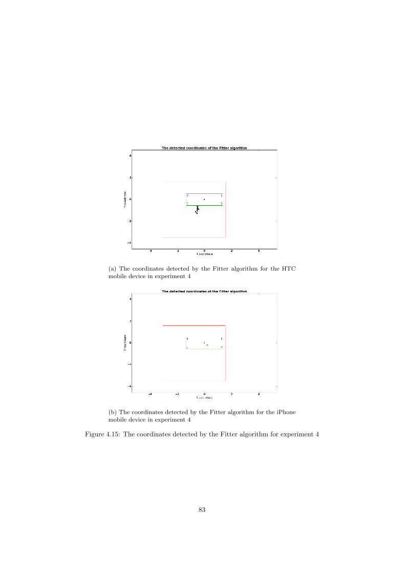
(a) The coordinates detected by the Fitter algorithm for the HTCmobile device in experiment 4

(b) The coordinates detected by the Fitter algorithm for the iPhonemobile device in experiment 4

Figure 4.15: The coordinates detected by the Fitter algorithm for experiment 4

83

4.2.4.1 Conclusions-experiment 4

– The idle mobile phones communicate far less with the drones com-pared to the ones in active state(experiment 1 and experiment 3)

– The number of points reconstructed in the iPhone case is muchsmaller than in the HTC case

– The Fitter algorithm did not reconstruct too many coordinates inthis experiment, even though there are more than 4 data packetsdetected by the drones

84

Chapter 5

The performance of theFitter algorithm

5.1 Introduction

In the previous chapter, we observed that the Fitter algorithm did notreconstruct the coordinates of the cell-phone in most cases even thoughthere was a sufficient number of packets(more than 4). In this chapter, wedecided to run the analysis of counting packets versus the states for theexperiments with data points(experiment 1, experiment 3, and experiment4), because we did not observe a consistent outcome of the Fitter acrossall of these experiments. A similar algorithm to the first part of the cut-offmodel was used, which computes the behavior of a device. The differenceis that the behavior is used for counting purposes for both the coordinatesand the packets. The results showed that there was a bug in the algorithm,which was later fixed.

The comparison between the coordinates and the raw packets containsseveral steps. Firstly, the number of packets per 10 second interval iscomputed, as well as the number of points calculated by the algorithm.Secondly, a binary variable called state is introduced in the case of thecoordinates for every 10 seconds time interval. The state is equal to one,if there were coordinates calculated for that particular device and timeinterval, and zero otherwise. Lastly, for each time interval of 10 seconds,the number of packets and the state are compared by means of a graphicalrepresentation. This graphical representation can indicate which intervalshave detections or not and packets or not.

For a better understanding of what actually happened, we decided toanalyze in parallel both the previous datasets and the current obtaineddatasets by looking at the following elements: the quantities that assessthe performance of the Fitter algorithm and the indicators regarding theefficiency of the Fitter algorithm and of the WiFi tracking system, respec-tively.

85

5.2 Quantities that assess the performanceof the Fitter algorithm

Several quantities were computed for each test and experiment in orderto evaluate the performance of the Fitter algorithm before and after thebug fix, which have a 0 index if they refer to the results prior to the bugfix(before), while 1 indexes refer to the results after the bug fix(after).

There are two types of quantities:

– related to the total number of packets(Records packets)

– related to the number of reconstructed data points by the Fitter(Records Fitter)

Three different categories were created for the comparison between datapackets and states which have as a measurement unit a number of 10seconds time intervals. The categories are the following:

– niFitter are the number of time intervals that have both points recon-structed by the algorithm and the number of data packets not equalto zero(state 6= 0 and Records packets 6= 0).

– ni0 are the number of intervals with no reconstructed points by theFitter, but with records different than zero in the raw dataset(state= 0 and Records packets 6= 0).

– ninopackets are the number of intervals with neither records in theraw dataset nor records reconstructed by the Fitter algorithm(state= 0 and Records packets = 0).

The sum of these should be equal to the the maximum number of timeintervals for a particular test, the intervals variable, which represents thenumber of time intervals of size 10 seconds that are between the arrivaland departure of a device or the start and end time of an experiment.

intervals = niFitter + ni0 + ninopackets

The arrivals and departures of the WiFi devices are quantified as follows:

– Arr interval pack, the number of the first time interval when themobile device sent packets to the routers and the timestart.

– Dep interval pack represents the number of remaining intervalsbetween the timestop and the last interval when the mobile devicesent packets to the routers

– Arr interval alg, the number of intervals between the interval offirst point detected by the algorithm and the timestart

– Dep interval alg, the number of intervals between the timestop andthe time of the last point detected by the algorithm

Other important quantities that are relevant for the performance are re-lated to the resolution of the Fitter algorithm:

86

– µx represents the average value of the x-coordinate for a particulartest and experiment

– µy represents the average value of the y-coordinate for a particulartest and experiment

– σx represents the root mean squared error of the x-coordinate for aparticular test and experiment

– σy represents the root mean squared error the y-coordinate for aparticular test and experiment

Eventually, the tracking system performance was evaluated quantitativelybased on the indicators below, which refer to the performance of the al-gorithm and to the performance of the WiFi tracking system.

Prob ddeted alg represents the probability that the algorithm computesthe points for a selected time interval of for example 10 seconds. Moreover,it is the fraction of the number of intervals with coordinates computed bythe Fitter algorithm(niFitter) divided by the number of time intervals withdata packets.

Prob ddeted alg =niFitter

niFitter + ni0

Efficiency wifi represents the probability that the WiFi tracking systemcommunicates during a time interval(e.g., 10 seconds). These statisticsare calculated within the entire measurement period [timestart, timestop].1

Efficiency wifi =niFitter + ni0

niFitter + ni0 + ninopackets

Efficiency wifi ui constitutes the probability that the WiFi tracking sys-tem communicates every selected time interval(e.g., 10 seconds) with themobile device within the time interval [Arrival, Departure], where theArrival represents the time interval when the first detection of a particulardevice was seen first, while Departure represents the time interval wherethe last detection of that particular devices was seen. Arr interval algrepresents the number of 10 seconds intervals of the difference betweenthe Arrival and timestart, while Dep interval alg represents the num-ber of 10 seconds intervals of the difference between the timestop andthe Departure. The Efficiency wifi and Efficiency wifi ui differwhen the Arrival and Departure of a WiFi device do not correspondto timestart and timestop.1

0

Efficiency wifi ui =niFitter + ni0

niFitter + ni0 + ninopackets −Arr interval alg −Dep interval alg1The reason why this interval is important is because sometimes the analyst is not able

to choose the exact moment when the first packets or coordinates were calculated by thealgorithm.

87

Total efficiency represents the probability of reconstructing the coordi-nates of the mobile devices given the performance of the WiFi trackingsystem for every selected time interval(e.g., 10 seconds).

Total efficiency = Prob ddeted alg × Efficiency wifi

Total efficiency ui is the probability of the Fitter reconstructing the co-ordinates for the mobile devices given its efficiency in the interval [Arrival,Departure]. This indicator should be compared with the Total efficiencyindicator.

Total efficiency ui = Prob ddeted alg × Efficiency wifi ui

5.3 Experiment 1

It is reminded that for this experiment, we tested the communicationbetween mobile devices and routers when the cell-phones are not connectedto the network. In this state, the mobile devices send probe packets.

In Table 5.1, a difference can be observed between the results before andafter the bug fix. Initially, the algorithm computed a smaller number ofrecords for each test, but after the algorithm was corrected the numberincreased(which is a good result). For example, the highest increase wasin Test 3 of this experiment, which initially had only 2 points calculated,but after fixing the bug there were 81 points added. As it can be seenin the same table, the number of intervals without packets is similar forall four tests except for test 2 which contains 3 time intervals of 10secondcompared to the rest which contain only 2 time intervals of 10 seconds.

When looking at the probability that the algorithm computes records(thiswas completely different from test to test prior the bug fix), but it in-creased afterwards to intervals of probability with the upper bound of100% for all four tests. Due to the fact that the arrival time and the timestart of the tests coincide, the Efficiency wifi and Efficiency wifi uicoincide. It is interesting to see that within this experiment almost all 10seconds contain data packets.

The Total efficiency and Total efficiency ui are different before andafter the bug fix as they depend on the probability that the algorithmcalculates points.

88

Statistics iPhone test1 iPhone test2 iPhone test3 iPhone test4Records F itter0 96 39 2 20Records F itter1 113 88 83 59Records packets 2,390 816 1,205 466

niFitter0 96 39 2 20niFitter1 113 88 83 59ninostates0 17 49 81 39ninostates1 0 0 0 0ninopackets0 2 3 2 1ninopackets1 2 3 2 1

Intervals 115 91 85 60Prob ddeted alg0 84.9%± 11.6% 44.3%± 18.1% 2.4%± 5.8% 33.9%± 21.2%Prob ddeted alg1 [99%, 100%] [98.7%, 100%] [98.6%, 100%] [98.1%, 100%]Efficiency wifi0 98.3%± 4.2% 96.7%± 6.5% 97.6%± 5.8% 98.3%± 5.8%Efficiency wifi1 98.3%± 4.2% 96.7%± 6.5% 97.6%± 5.8% 98.3%± 5.8%Efficiency wifi ui0 98.3%± 4.2% 96.7%± 6.5% 97.6%± 5.8% 98.3%± 5.8%Efficiency wifi ui1 98.3%± 4.2% 96.7%± 6.5% 97.6%± 5.8% 98.3%± 5.8%Total efficiency0 83.5%± 12.0% 42.9%± 18.0% 2.4%± 5.8% 33.3%± 21.2%Total efficiency1 98.3%± 4.2% 96.7%± 6.5% 97.6%± 5.8% 98.3%± 5.8%

Total efficiency ui0 83.5%± 12.0% 42.9%± 18.0% 2.4%± 5.8% 33.3%± 21.2%Total efficiency ui1 98.3%± 4.2% 96.7%± 6.5% 97.6%± 5.8% 98.3%± 5.8%

µx0(m) -0.9 0.4 0.4 -0.2µx1(m) -1.1 -1.3 -71.6 0.5µy0(m) 0.0 -0.1 0.3 0.0µy1(m) 0.2 -1.2 -5.1 0.7σx0(m) 0.6 1.0 0.7 0.8σx1(m) 0.9 2.0 501.4 0.8σy0(m) 0.3 0.7 0.2 0.8σy1(m) 0.8 3.7 41.2 1.5

Table 5.1: Statistics of experiment 1 iPhone(before(0) and after(1) fix results)

5.3.1 Test 1

In the Figure 5.1, the comparison between the states and the data packetscan be seen and the 10 seconds time intervals which have detections ornot. Figure 5.1a shows whether there were detections for this particularbefore the bug fix, while Figure 5.1b shows the improvement. The laterfigure reveals that two time intervals of 10 second have no packets, whilethe rest of the intervals all have detections. Test 1 represented the testwith the largest number of points calculated by algorithm before the bugfix, but, after the fix, the 17 more points were detected.

According to the Table 5.1, even though there were much more pointsthe performance of the average x and y coordinates decreased. Initially,the average x coordinate was −0.9 ± 0.6 and the average y coordinatewas 0.0± 0.3 for this test. However, after the correction both values hadvalues further away from 0, the reference point for both coordinates, andtheir spreads(σx and σy increased as well). Hence, there was an increase

89

in detection efficiency, but this increase did not improve the precision inresolution.

When looking at Figure 5.2, the coordinates calculated by the algorithmare plotted. The red rectangle represents the area of the room, whilethe green rectangle represents the area of the table on which the mobiledevice was placed. It can be seen that the points detected before the bugfix are still present in the plots after the fix. Figure 5.2b reveals additionalpoints, which are in the area of the room, but are not located on the table.This is in accordance with the fact that there were improvements from anumber of data points calculated, but this did not bring any increase theaccuracy of the detections for both x and y. One can see 3 main areaswith multiple data points. On one hand, there is a cluster of points thatlocated on the table, but shifted to the left side of the center of referencewith the y coordinate close to 0. On the other hand, there are two otherareas with points in the room, but not on the table. These points areeither located in the vicinity of Charlie and Echo routers, but with theiry coordinate close to 0 or in the middle between the Charlie and Foxtrotrouters, but with their x coordinate close to 0. According to Table 4.3,the Foxtrot, Echo, and Charlie routers had the highest signal strength.The algorithm uses this information and fits the signals according to theirmagnitude. Thus, the calculated points will be closer to the router witha higher signal strength. The orientation of the mobile device might nothave a large impact on the reconstruction of the coordinates compared tothe recorded signal strength.

90

(a) The comparison between the states and data packets for experi-ment 1 Test 1(before)

(b) The comparison between the states and data packets for experi-ment 1 Test 1(after)

Figure 5.1: The comparison between the states and data packets for experiment1 Test 1 before and after

91

(a) The calculated coordinates by the Fitter algorithm experiment 1Test 1 (before)

(b) The calculated coordinates by the Fitter algorithm experiment 1Test 1 (after)

Figure 5.2: The calculated coordinates by the Fitter algorithm experiment 1Test 1(before and after)

The rest of the tests and the results of their analyses can be found in theAppendix in section A.6

5.4 Experiment 3

We remind the reader that experiment 3 was performed in order to analyzethe way the mobile devices communicate when an app is used. There

92

were two main mobile devices used HTC and iPhone, which were testedunder the same conditions and for the same amount of time. From anumber of packets perspective, according to Tables 5.2 and 5.3, the HTCcommunicates less with the routers than the iPhone which can be observedgiven the number of recorded packets per test for each device. Therefore,a higher number of points was expected to be computed in the iPhonecase. However, this only occurred for tests 1 and 4. Moreover, for tests 2and 3, the HTC contained much more points than the iPhone.

After the Fitter algorithm was fixed, the number of calculated points wassimilar except for test 3, where for the iPhone device were computed 95points compared to the 94 number of points calculated for the HTC. Thisresult is reassuring as this may indicate that the device type may notinfluence the number of points calculated by the algorithm. In addition tothis, the total efficiency of the tracking system is very high for both devices.It can be also seen that the average values of the x and y coordinates didnot significantly change. This is a positive result compared to the valuesobtained in experiment 1, where the resolution deprecated.

Statistics HTC test1 HTC test2 HTC test3 HTC test4Records packets 62,285 62,274 72,112 57,403


Intervals 97 97 97 97Prob ddeted alg0 43.8%± 17.5% 10.4%± 10.8% 26%± 15.5% 65.6%± 16.8%Prob ddeted alg1 97.9%± 5.1% 99.0%± 3.5% 97.9%± 5.1% 97.9%± 5.1%Efficiency wifi0 99.0%± 3.5% 99.0%± 3.5% 99.0%± 3.5% 99.0%± 3.5%Efficiency wifi1 99.0%± 3.5% 99.0%± 3.5% 99%± 3.5% 99.0%± 3.5%Efficiency wifi ui0 [98.2%, 100%] [98.2%, 100%] [98.2%, 100%] [98.2%, 100%]Efficiency wifi ui1 [98.2%, 100%] [98.2%, 100%] [98.2%, 100%] [98.2%, 100%]Total efficiency0 43.3%± 17.5% 10.3%± 10.7% 25.7%± 15.4% 64.9%± 16.8%Total efficiency1 96.9%± 6.1% 97.9%± 5.1% 96.9%± 6.1% 96.9%± 6.1%

Total efficiency ui0 43.8%± 17.5% 10.4%± 10.8% 26%± 15.5% 65.6%± 16.8%Total efficiency ui1 97.9%± 5.1% 99.0%± 3.5% 97.9%± 5.1% 97.9%± 5.1%

µx0(m) 0.9 1.3 0.9 -0.1µx1(m) 1.0 1.3 0.9 -0.2µy0(m) -0.8 -0.7 -0.6 -0.6µy1(m) -1.0 -0.8 -1 -0.9σx0(m) 0.0 0.1 0.1 0.3σx1(m) 0.1 0.1 0.1 0.3σy0(m) 0.1 0.1 0.2 0.2σy1(m) 0.1 0.0 0.2 0.5

Table 5.2: Statistics of experiment 3 HTC(before(0) and after(1) fix results)

93

Statistics iPhone test1 iPhone test2 iPhone test3 iPhone test4Records packets 94,200 91,441 90,581 93,495


Intervals 97 97 97 97Prob ddeted alg0 69.8%± 16.2% [0%, 1.2%] 2.08%± 5.0% 96.9%± 6.1%Prob ddeted alg1 97.9%± 5.1% 99.0%± 3.5% 99.0%± 3.5% 97.9%± 5.1%Efficiency wifi0 99.0%± 3.5% 99.0%± 3.5% 99.0%± 3.5% 99.0%± 3.5%Efficiency wifi1 99.0%± 3.5% 99.0%± 3.5% 99.0%± 3.5% 99.0%± 3.5%Efficiency wifi ui0 [98.8%, 100%] [98.8%, 100%] [98.8%, 100%] [98.8%, 100%]Efficiency wifi ui1 [98.8%, 100%] [98.8%, 100%] [98.8%, 100%] [98.8%, 100%]Total efficiency0 69.1%± 16.3% [0%, 1.2%] 2.1%± 5.1% 95.9%± 7.0%Total efficiency1 96.9%± 6.1% 97.9%± 5.1% 96.9%± 6.1% 96.9%± 6.1%

Total efficiency ui0 69.8%± 16.2% [0%, 1.2%] 2.1%± 5.1% 96.9%± 6.1%Total efficiency ui1 97.9%± 5.1% 99.0%± 3.5% 99.0%± 3.5% 97.9%± 5.1%

µx0(m) 0.7 - 0.4 0.3µx1(m) 0.4 1.2 1.0 0.3µy0(m) -0.1 - 0.1 -0.9µy1(m) 0.4 -1.2 -1.0 -0.9σx0(m) 0.3 - 0.4 0.0σx1(m) 0.5 2.2 0.2 0.0σy0(m) 0.2 - 0.3 0.1σy1(m) 0.8 1.0 0.3 0.2

Table 5.3: Statistics of experiment 3 iPhone(before(0) and after(1) fix results)

5.4.1 Test 1

In this test, there was a significant difference from a number of computedpoints perspective. Thus, as previously seen, where there were packets thealgorithm was able to compute points for the majority of the 10 time in-tervals which contained data packets, except for 2 for both mobile devices.Besides this, it could be seen that there existed a time interval which didnot contain both packets and calculated points. This can be visualized inFigure 5.3 for the HTC case and in Figure 5.5 for the iPhone.

5.4.1.1 HTC

The plots of the coordinates(Figure 5.4) show that a cluster of pointswas formed in the vicinity of router Delta. According to the results ofexperiment 3 Test 1( Subsubsection 4.2.3.1), the Delta delta drone hadon average the highest signal strength. Thus, one potential explanationfor the location of the points calculated by the algorithm is that the highaverage signal strength of recorded by this drone which seems to influencethe algorithm.

94

Another interesting aspect can be seen in Figures 5.3a and 5.3b, wherethere seems to be no significant difference between the results obtainedprior to the bug fix and current ones besides the increased number ofpoints obtained in the later. However, the majority of these points arelocated outside the area of the table, but still in the room.

5.4.1.2 iPhone

In Test 1 of the iPhone, a similar situation as in the HTC case occurs,where the main cluster of points was maintained after the algorithm wasfix(Figure 5.6). This cluster contains as well points that are close to theDelta drone as in the HTC case, but these points are located closer to thereference point for the y coordinate. Besides the main cluster, there canbe also points that are located both outside the area of the table and thearea of the room. These are outliers, which seem to have the x coordinateclose to 0. One potential explanation may be that the distribution of thesignal strength of the Beta router overlapped with the one obtained for theDelta drone(Subsubsection 4.2.1) and may have influenced the calculatedcoordinates.

95

(a) The states and coordinates detected by the Fitter algorithm forthe HTC mobile device experiment 3 Test 1(before)

(b) The states and coordinates detected by the Fitter algorithm forthe HTC mobile device experiment 3 Test 1(after)

Figure 5.3: The states and coordinates detected by the Fitter algorithm for theHTC mobile device experiment 3 Test 1

96

(a) The calculated coordinates by the Fitter algorithm for the HTCmobile device experiment 3 Test 1(before)

(b) The calculated coordinates by the Fitter algorithm for the HTCmobile device experiment 3 Test 1(after)

Figure 5.4: The calculated coordinates by the Fitter algorithm for the HTCmobile device experiment 3 Test 1(before and after)

97

(a) The states and coordinates detected by the Fitter algorithm forthe iPhone mobile device in experiment 3 Test 1(before)

(b) The states and coordinates detected by the Fitter algorithm forthe iPhone mobile device in experiment 3 Test 1(after)

Figure 5.5: The states and coordinates detected by the Fitter algorithm for theiPhone mobile device in experiment 3 Test 1(before and after)

98

(a) The calculated coordinates by the Fitter algorithm for the iPhonemobile device experiment 3 Test 1(before)

(b) The calculated coordinates by the Fitter algorithm for the iPhonemobile device experiment 3 Test 1(after)

Figure 5.6: The calculated coordinates by the Fitter algorithm for the iPhonemobile device experiment 3 Test 1(before and after)

The rest of the tests and the results of their analyses can be found in theAppendix in section A.7

5.5 Experiment 4

Experiment 4 was performed for both the HTC and iPhone at the sametime in order to get insight in how mobile devices communicate with the

99

routers when they are in an idle state. This experiment was important,because the idle state is the most common state of a mobile device. In-teresting information could be drawn out of this experiment. Initially,the algorithm could barely compute points for the mobile devices. Thus,according to Table 5.4, the initial probability was 30.9% ± 16.3% for theHTC compared to 4.6% ± 7.4% for the iPhone, these results changed tothe intervals of probability [98.4%, 100%] and [95.1%, 100%], respectively,after the algorithm was fixed. Nevertheless, the efficiency of the trackingsystem scored initially 18.8%±13.8% for the HTC mobile device and only6.1% ± 8.4 for the iPhone. This seems to be a poor result compared toexperiment 1 and 3 which had data packets in the majority of the 10 sec-onds time intervals. This may mean that the mobile devices send fewerpackets and tracking seems a challenge when they are in an idle state.

The main difference could be seen from a number of points computed forboth mobile devices. According to Table 5.4, there were in the end 68points for the HTC and 22 points calculated for the iPhone. These con-stituted points for all the intervals which contained data packets. From acoordinate perspective, the results after the algorithm was fixed revealedthat the average x and y coordinates of the HTC mobile device did notdiffer compared to the ones initially obtained, but they were slightly in-creased. However, in the iPhone case, there was a significant change as 21points more were calculated. For example, the average x coordinate was0.6± 0.2, while the average y coordinate was −1.3± 0.3.

100

Statistics HTC iPhoneRecords packets 3565 3167

niFitter0 21 1niFitter1 68 22ninostates0 47 21ninostates1 0 0ninopackets0 293 339ninopackets1 293 339

Intervals 361 361Prob ddeted alg0 30.9%± 16.3% 4.6%± 7.4%Prob ddeted alg1 [98.4%, 100%] [95.1%, 100%]Efficiency wifi0 18.8%± 13.8% 6.1%± 8.4%Efficiency wifi1 18.8%± 13.8% 6.1%± 8.4%Efficiency wifi ui0 18.9%± 13.8% 6.4%± 8.6%Efficiency wifi ui1 6.1%± 8.4% 18.8%± 13.8%Total efficiency0 18.8%± 13.8% 0.3%± 1.9%Total efficiency1 18.8%± 13.8% 6.1%± 8.4%

Total efficiency ui0 5.9%± 13.8% 0.3%± 1.9%Total efficiency ui1 18.9%± 13.8% 6.4%± 8.6%

µx0(m) -0.5 0.2µx1(m) -0.6 0.6µy0(m) -0.9 -0.2µy1(m) -1.3 -1.3σx0(m) 0.1 0.0σx1(m) 0.2 0.2σy0(m) 0.2 0.0σy1(m) 0.3 0.3

Table 5.4: Statistics of experiment 4 HTC and iPhone (before(0) and after(1)fix results)

5.5.1 HTC

According to Figure 5.8, it can be seen that the initial cluster of pointswas increased after the algorithm was repaired. In addition to this, theposition of the cluster is between the Charlie and Delta routers, on the leftside of the reference point, very close to the area of the table and inside theroom. In addition to this, the additional points seem to be more scatteredthan the initial ones. One potential explanation for this shift to the leftside may be that the Charlie router had on average the highest signalstrength, followed by the Delta and Beta(very close to Delta).

101

(a) The states and coordinates detected by the Fitter algorithm forthe HTC mobile device in experiment 4(before)

(b) The states and coordinates detected by the Fitter algorithm forthe HTC mobile device in experiment 4(after)

Figure 5.7: The states and coordinates detected by the Fitter algorithm for theHTC mobile device in experiment 4(before and after)

102

(a) The reconstructed coordinates by the Fitter algorithm for theHTC mobile device experiment 4(before)

(b) The reconstructed coordinates by the Fitter algorithm for theHTC mobile device experiment 4(after)

Figure 5.8: The reconstructed coordinates by the Fitter algorithm for the HTCmobile device experiment 4(before and after)

5.5.2 iPhone

Figure 5.92 presents the comparison between the performance of the pointsbefore and after the algorithm was fixed. As mentioned before, the algo-rithm initially computed only one point for this experiment, which could

2This figure was separated in two plots, because the matplotlib package for python some-times shrinks the image and the time intervals with detections do not overlap with the oneswith detections

103

be seen in the first time interval of 10 seconds with data packets. Thisseemed a poor result given the existence of sufficient data packets for therest of the 21 time intervals. However, the new results seemed encouragingas one could draw the conclusion that if there are more than 4 availabledata packets in a time interval, then the algorithm may compute a datapoint.

From a coordinate perspective, Figure 5.10 shows that a cluster of pointsoutside the area of the table was added to the point found inside it afterfixing the algorithm. This cluster is positioned on the right side of thereference point in the vicinity of the Delta router. This indicates as previ-ously seen that even though the number of points increased, this did notmean that the performance improved as well. According to the resultsof experiment 4 for the iPhone case, the highest signal strength could befound in the case of Delta followed by Charlie which may have influencedthe position of the computed data points.

104

(a) The states and coordinates detected by the Fitter algorithm forthe iPhone mobile device in experiment 4(before)

(b) The states detected by the Fitteralgorithm for the iPhone mobile devicein experiment4(after)

(c) The packets for the iPhone mobiledevice in experiment4(after)

Figure 5.9: The states and coordinates detected by the Fitter algorithm for theiPhone mobile device in experiment 4

105

(a) The reconstructed coordinates by the Fitter algorithm for theiPhone mobile device experiment 4(before)

(b) The reconstructed coordinates by the Fitter algorithm for theiPhone mobile device experiment 4(after)

Figure 5.10: The reconstructed coordinates by the Fitter algorithm for theiPhone mobile device experiment 4(before and after)

106

5.6 Conclusions

From the results of the experiments before and after the bug fix of theFitter algorithm, the following conclusions can be drawn:

– The number of points reconstructed by the Fitter algorithm has in-creased significantly after the bug fix(e.g, a higher reconstructionefficiency)

– The accuracy of the average x and y coordinates is changed, but itwas not improved in the majority of the cases

– The efficiency of the WiFi system and the efficiency of calculatingcoordinates have increased significantly

– There is a high probability that the Fitter algorithm is able to recon-struct the coordinates of the mobile devices if there are more than 4data packets from 4 different drones

– Depending on the experiment and on the test, the extra reconstructedpoints by the Fitter are either points in the vicinity of the referencepoint or outliers

– WiFi tracking may be challenging in idle states of mobile devices

– Strategies need be developed for increasing the communication be-tween mobile devices and drones

107

Chapter 6

Features of the systemand comparison withother projects

In this chapter, the KPMG LAS system is compared with projects found inthe literature by following the framework of Mautz[34] which contains theuser and technical requirements an indoor positioning application shouldhave. Crucial elements need to be taken into consideration according toMautz[34] when actually designing and implementing an indoor position-ing application. These requirements are shown in Figure 6.1a and Figure6.1b. These figures show the multi-dimensionality of the optimizationproblem that the companies are confronted with.

(a) User requirements for indoor posi-tioning systems(Mautz[34])

(b) Technical parameters for indoorpositioning systems(Mautz[34])

6.1 Business-user requirements

Mautz[34] describes briefly each user requirement as follows in Figure 6.1a:

108

– accuracy (mm, cm, dm, meter, decameter level)

– coverage area/limitations to certain environments (single room,building, city, global)

– cost (unique system set-up costs, per user device costs, per roomcosts, maintenance costs)

– required infrastructure (none, markers, passive tags, active beacons,pre-existing or dedicated, local or global)

– market maturity (concept, development, product)

– output data (2D or 3D coordinates, relative, absolute or symbolicposition, dynamic parameters such as speed, heading, uncertainty,variances)

– privacy (active or passive devices, mobile or server based computa-tion)

– update rate (on-event, on request or periodically e.g., 100Hz oronce a week)

– interface (man-machine interfaces such as text based, graphical dis-play, audio voice and electrical interfaces such as RS-232, USB, fiberchannels or wireless communications)

– system integrity (operability according technical specification, alarmin case of malfunction)

– robustness (physical damage, theft, jamming, unauthorized access)

– availability (likelihood and maximum duration of outages)

– scalability (not scalable, scalable with area-proportional node deploy-ment, scalable with accuracy loss)

– number of users (single user e.g., total station, unlimited users e.g.,passive mobile sensors)

– intrusiveness/user acceptance (disturbing, imperceptible)

– approval (legal system operation, certification of authorities)

Several user requirements are discussed here in more detail with respectto the ones presented by Mautz. These requirements are the following:accuracy, coverage, market maturity, integrity, availability, update rate,system latency, interface, data output, privacy, costs, and number of users.

Accuracy

The accuracy requirement represents the most important measure, if it isviewed from a user perspective. In order to compare system performances,a useful metric for the quality of positions is the computation of the stan-dard deviation(RMSD-Root Mean Squared Deviation or RMSE-Root MeanSquared Error):

σP =

√√√√ 1

n

n∑i=1

(Pi − Pi)2

109

,

where n is the number of estimated position vectors Pi and Pi the positionvector predicted by a modal of the localized node i, or, if only one singlelocation is estimated, Pi is replaced with a single position vector P0.

Low accuracy can be defined as the standard deviation σP > 10m andhigh accuracy as σP < 1cm. Even though, the accuracy represents a keydriver for most applications. It should be viewed in the context with theother performance parameters.

The main metric used for evaluating the accuracy of the KPMG WiFitracking system is the root mean squared error(RMSE) like the metricproposed by Mautz. According to the results of the experiments andthe CHEP data, the RMSE differs by experiment and test. Due to thefact that the coordinates are calculated by means of the Fitter algorithmin Chapter 3, Chapter 4, and Chapter 5, the main factor that affects thequality of the results represents the recorded signal strength by the drones,which is influenced itself by several factors. Other factors that also playa key role are the following: device type, device state, position of themobile device, shape of the area under analysis, and the configuration ofthe drones, etc.

The results obtained from the CHEP conference showed that the accu-racy for a lying still on a table iPad device was 7.8m for the x coordinateand 6.4m for the y coordinate. However, the results obtained from theexperiments revealed a RMSE smaller than 1m. Nevertheless, these ex-periments where performed with the drones close to the mobile(WiFi)devices. It might be that the mobile(WiFi) devices are detected with ahigher RMSE as long as it is not close to the drones.

It may be the case that the results obtained for the CHEP data have largerRMSE values of the x and y coordinates. This assumption is made basedon the validation experiments which revealed that after the bug fix, theRMSE increased. Verifying this assumption was not possible, because anew dataset of the CHEP could not be obtained after the bug fix and,thus, the models could not be applied.

The KPMG LAS system is compared with similar projects from the liter-ature and public information of the main competitors. From a literatureperspective, Bahl and Padmanabhan’s system RADAR[20] has an accu-racy of 2 − 3m. From a competitors’ perspective, an indoor positioningsystem developed by Polestar company represents NAO Campus, whichpromises an accuracy that ranges from 2.1m up to 5m[27]. The Infsoftcompany promises on their website[32] an accuracy of 1m. 1

Coverage

The coverage describes the spatial extension where system performancemust be guaranteed by a positioning system. One of these categoriesshould be specified:

1It may be the case that the public information of the main competitors is not reliable forcomparison due to marketing strategies.

110

– Local coverage - small, well-defined, limited area which is not ex-tendable

– Scalable coverage - systems with the ability to increase the areaby adding hardware(deployment of additional sensors)

– Global coverage - system performance worldwide or within the de-sired/specified area. Only the GNSS systems and celestial navigationbelong in this category

The coverage area is dependent mainly on the detected signal strength ofthe mobile devices and the environmental limitations within this area. Theenvironmental limitations are the elements such as windows, furniture,and walls that may interfere with the way the signal strength is recorded.Our experiments showed that sometimes these obstacles could increase ordecrease the magnitude of the signal strength.

According to Subsection 4.2.2, more than 30 meters distance was enoughto detect a mobile device. Nevertheless, the 30 meters were measured ona hallway where there were no obstacles. This value may change if theseenvironmental limitations stand in the way. When comparing with theliterature, Nuaimi and Kamel[12] argue that the range of existing systemsgo from 5 to 50 meters, as providing a system with a coverage of morethan 60 is very challenging.

The category in which the KPMG WiFi tracking system belongs to is thescalable coverage systems, the systems with the ability o increase the areaunder analysis by adding drones. If we assume that the area under analysishas a square shape(the distance between the drone and the WiFi deviceis equal to 30m and half of the diagonal of the room) and based on theresults of the experiments, then the coverage area may be approximately1800m2.

Market maturity

The KPMG WiFi tracking system has been developed for less than 6months from a market maturity perspective. It represents a productin development as it is tested only in small experiments like the onesdeveloped within this work. Even though the performance seems to bepromising, this products needs more testing in a real-life environment.For example, the system will be tested at the KPMG canteen.

Integrity

Integrity relates to the confidence which can be placed in the output of asystem. Integrity risk is the probability that a malfunction in the systemleads to an estimated position that differs from the required position bymore than an acceptable amount(the alarm limit) and that the user is notinformed within the specified period of time(time-to-alarm).

According to Mautz[34], regulator bodies have studied and defined in-tegrity performance parameters in some sectors such as civil aviation,however, in other sectors, including those relating to indoor navigationit is more difficult to find quantified integrity parameters.

111

Availability

Availability is the percentage of time during which the positioning serviceis available for use with the required accuracy and integrity. This may belimited by random factors (failures, communications congestion) as well asby scheduled factors(routine maintenance). Generally, one of the followingthree levels could be specified, although this will depend on the particularapplication:

1. low availability: < 95%

2. regular availability: > 99%

3. high availability: > 99.9%

To achieve availability, it is assumed that continuity, accuracy, and in-tegrity requirements are fulfilled. Application descriptions usually includespecification of availability, whereas system developers usually do not spec-ify an availability figure.

As mentioned before, the KPMG LAS represents an experimental projectwhich has not yet extensively been tested in a real-life environment. Thismeans that assessing the availability of the system is difficult. However, itcan be affirmed that the entire system was tested at the CHEP conferencefor 4 days in row and it was affected by random factors such as failures andcongestion problems leading to a low availability. Due to the fact, thatthis project represents a pilot, the desire is to increase the availability to> 99.9%.

Update rate

The update rate is the frequency with which the positions are calculatedon the device or at an external processing facility. The following types ofmeasurements rates exist:

1. periodic: regular update, specified in an interval (unit e.g., (Hz) )

2. on request: triggered by the user or by a remote device.

3. on event: measurement update initiated by the local device whena specific event occurs, e.g., when a temperature sensor exceeds acritical threshold.

The KPMG WiFi system has an update rate of 10 seconds in which thepositions are calculated. From a measurement rate type, this system entersin the periodic category as it synchronizes with the way the algorithmswork, which, as mentioned before, use a buffer of 10 seconds time intervalto compute the coordinates of a mobile device. From the rate of updateperspective, it would be good in the future if the 10 second time intervalis lowered to a smaller time interval. It may the case that the accuracy ofthe coordinates may be improved and the rate of update will be faster.

The update rate may suffer modifications depending on the tracking type,“static” or in “motion”. On one hand, if the tracking type is static(thedevice does not move), more data packets may be needed to increase the

112

accuracy of the detections. On the other hand, if the tracking type is inmotion(device is moving), then there are less data packets per unit time,which may decrease the accuracy of the coordinates.

System latency

The system latency describes the delay with which the requested informa-tion is available to the user. The latency can have the following values:

– real time: Does not tolerate “perceivable” delays. It is the mostdemanding latency requirement. It is necessary for navigation andalmost all indoor positioning applications.

– sooner the better: Requires the system’s best effort.

– sooner the better with an Upper Limit: Requires the system’s besteffort but the system must be designed to limit the maximum delayto a specified threshold.

– post processing: No specific time of delivery is defined.

When looking at the system latency perspective, the information re-lated to what the main areas of interest are. The heatmap uses the re-constructed coordinates of the algorithm. Thus, the delay represents onlyfrom the amount of time it takes to the algorithm in order to computethe coordinates of the mobile device. The KPMG system may enter thepost-processing category.

Interface

The KPMG LAS platform contains a user-friendly web interface/dash-board which consists of several parts. The heatmap plays a key role. Ithas on the background the floor plan of the area of coverage. On thisfloor plan, the areas where the mobile devices are detected are plotted.The heatmap shows this activity on an aggregated level and not on anindividual device level. This way the privacy element is handled properlyas the intention is only to count the number of devices in the areas ofinterest. These areas of interest enable the clients identify whether thecurrent display layout is attractive enough for the clients, what are themost interesting and visualized products by the visitors, and where theclients spend more time e.g., at the cash-register, in a queue, etc.

The KPMG LAS dashboard also provides statistics with respect to thenumber of visitors in the area, as well as an intuitive plot which showshow this number varies in time. As well as, the percentages of the clientssplit by areas of interests are shown by means of a pie chart plot. Inaddition to this, the box-plot indicates the dwell time of the visitors andthe results are presented on aggregated level.

Data output

The output data of the KPMG LAS platform contains 2D data withonly x and y coordinats that are visualized on an aggregated level in the

113

heatmap, as well as the timestamp, the errors for the coordinates of thealgorithm. It is foreseen that the z coordinates is also calculated by thealgorithms. At the moment, the z coordinate is equal to 0, thus it mightaffect the accuracy of the computed coordinates. In addition to this, notall the mobile devices are located on the same axis.

Privacy

KPMG has put a lot of effort in ensuring that the data privacy is handledcarefully. The KPMG LAS platform is designed to comply with the DutchData Protection Directive and contains a number of measures to ensurethat it is virtually impossible to identify a single individual. In addition tothis, the KPMG LAS platform provides opt-out(in) capabilities for thoseindividuals who do not wish to be tracked. The system filters out theopt-out devices and retains only the ones that are opt-in. A randomiser isalso forseen to be implemented which adds a random perturbation/statis-tical noise to the results of the analyses making the identification processvirtually impossible(Aircloak).

Number of users

The web-interface of the KPMG LAS platform can be accessed by multipleusers at the same time. However, the maximum number of users has notbeen assessed yet. Each user requires a username and a password in orderto log in to the system.

6.2 Technical parameters

Besides, the user requirements which refer mainly to the companies in-terested in purchasing the IPA(Indoor positioning applications), there arestill some technical parameters that need to be taken into consideration.Mautz described these as the following:

– level of hybridization(single modality, two different sensors, highlyhybrid sensor fusion).

– technology(optical, inertial, magnetic, sound etc.)

– measured quantity(direction, distance, signal amplitude, accelera-tion, time)

– basic measuring principle ((tri)lateration, (tri)angulation, fingerprint-ing, cell of origin, dead-reckoning)

– positioning algorithm used (multidimensional scaling, multilatera-tion, heuristics)

– signal used (sound waves, electromagnetic waves, magnetic field strength)

– signal wavelength (visible light, infrared, radio frequencies)

– system architecture (central or distributed systems)

– application (navigation, surveying, industry tracking, metrology)

114

– coordinate reference (local, global, object or sensor coordinate sys-tem)

According to the same author[34], the values of the performance param-eters are sometimes not determinable, because they depend on variousfactors, circumstances, and conditions. The definitions of the positioningrequirements parameters according to the same thesis[34] are presented,in order to have a reference point of how these systems should typicallybehave.

From a technical requirements’ perspective, the following requirementsperspective the following will be taken into consideration: technology,basic measuring principle, application, and signal strength.

Technology

The technology for the KPMG LAS is based on the detection of the WiFisignals, data that are recorded by the WiFi drones and that are sent to theKPMG Analytics Visualization and Environment Platform(KAVE), wherethe data is stored, validated, and calibrated. The output data obtainedfrom the algorithms is visualized on a dashboard in a web-interface.

Basic measuring principle

The main measuring principle is trilateration, which represents a techniquefor identifying the location of a device if the distances of at least threereferences are known. The Fitter algorithm combines the trilaterationtechnique with nonlinear Chi-square fit and Newton-Rapson techniqueto estimate the best possible parameters for the non-linear relationshipbetween the signal strength and the distance[55].

Application

There are multiple applications of the KPMG LAS to the business side.Firstly, the interest areas are revealed based on which customer pathscan be identified. Both enhance the understanding of the customer base.In addition to this, a new store layout can be optimized. For example,the visitors/customers may find in their way products that are sold inassociations with the most purchased ones or they may be “required” tofollow a different path in their way to certain products. These productscan be determined based on the market basket analysis technique. Suchtechniques offer insight in the relationships between products that arepurchased together. This insight combined with the information extractedfrom the WiFi tracking system can be used for customer profiling andtargeted advertising.

Due to privacy restrictions, the tracking system will not be evaluated onan individual device level to control to which extend the individual datais used. However, besides the opt-out feature, KPMG also supports anopt-in feature for clients who would like to be contacted after since they

115

are interested in a certain product and they would like to have much moreinformation.

6.3 Conclusion regarding the system

The performance of the KPMG LAS platform was evaluated from bothbusiness and technical perspectives. This system is currently a pilot whichseems to have a lot of potential. From a business perspective, this systembrings insight into the interest areas of the customers, an estimation ofthe number of detected devices, and several other statistics relevant formatching product offers to customers.

6.4 Implications of Apple’s decision to im-plement random Mac address on iOS8

At the Apple Worldwide Developers Conference in June 2014, David Stitesand Katie Skinner announced the changes of the WiFi scanning behaviorin the iOS8. It will will use random, locally administrated MAC addressesfor probe requests(sub-type 0x4) and responses(sub-type 0x5). Accordingto Apple’s product security and privacy representatives’ presentation[47],the MAC address used for the WiFi scans may not always be the devices’real(universal) address.

In this section, the potential implications of these changes are evaluated.Greg Sterling from Marketingland[53] believes that these decisions aremainly targeted such that Ad networks, WiFi hotspots, and other thirdparties will not be able anymore to have access to the real MAC IphoneiOS 8 and to combine them with other datasets. Thus, individuals cannotbe associated anymore with particular locations for later re-targeting. Itmay also be the case that Apple tries to get people’s consent that theirMAC addresses can be used.

Another potential implication of this change may affect the statistics re-lated to the dwell time of the Iphone mobile devices that are not connectedto the network. However, this will not have implications on the countingprocess, if the devices are connected to the WiFi network. In this case,the MAC address is not random anymore and all the statistics can becalculated based on that. In addition to this, the Android mobile devicesare not affected by this decision. The main competitors in the indoor/out-door positioning industry surprisingly support this decision even thoughthis may influence the various analyses that are performed.

It may be the case that Apple tries to increase their market share byattracting potential clients that are concerned with privacy. However, thecompany has bought in 2013 the WifiSlam start-up. They built for indoorpositioning technologies that pinpoint the location of the smartphone(andthe location of your friends) in real-time with an accuracy of 2.5m by usingonly ambient WiFi signals that are already present in buildings. Besidesthis, they developed location-based mobile apps that could engage with

116

users at the scale that personal interaction actually took place. Otherapplications ranged from step-by-step indoor navigation, to product-levelretail customer engagement, to proximity-based social networking.

117

Chapter 7

Contributions,limitations, conclusions,recommendations

7.1 Contribution to the literature

This work analyzes the performance of a new WiFi tracking system for lo-cation aware services from both business and technical perspectives. In theliterature, most projects for location aware services are small pilot projectsthat do not involve large amounts of data. Instead, in this research datawere analyzed from both real-life environment(CHEP conference), but alsocontrolled experiments which zoomed in and described how mobile devicescommunicate with the drones in different situations. The most importantfactors that influence the way the coordinates are calculated in controlledenvironments were identified based on the literature and on the controlledexperiments.

This research also proposes a strategy for analyzing the performance ofthe WiFi tracking systems by looking at the most important statisticsboth on individual and aggregated levels, which could not be found in theliterature. It evaluates into depth the performance of the algorithms andproposes models for calculating the probability of detecting mobile devices.In addition to this, a visualization over time, statistics, and indicators arecreated to assess the performance of the WiFi tracking system and thealgorithms.

From a business perspective, this study analyzes the WiFi tracking systembased on the framework proposed by Mautz[34] for indoor positioningalgorithms. In addition to this, it contains information related to themain competitors on the indoor tracking industry, but also projects fromthe literature.

118

7.2 Limitations

This research has several limitations which are explained chronologically.

One of the main limitations within Chapter 2 was that the CHEP datasetsused for analysis lacked relevant data which could be used for the analysis.Therefore, the accuracy was evaluated only based on one device(an iPaddevice). In addition to this, the actual coordinates of the iPad devicemay not be correctly calculated. This may have an impact on the biasof the average coordinates for both x and y coordinates. For a betterunderstanding of how this WiFi tracking system works, the entire trackingsystem should be tested in a real-life environment and on several moredevices which have their states and positions known.

In Chapter 3, two models were proposed for computing the probability ofdetecting mobile devices. The probability of detecting the mobile deviceswas calculated on a 5 minute level, but also on a 10, 30, and 60 secondlevel. The results of the models were obtained based on the datasets fromthe old version of the Fitter algorithm which had a bug. Due to thisbug, the algorithm did not compute all the points even though there weresufficient available data packets. It may be the case that the results ofthe models are obsolete and that the probability as well as the indicatiorsmay increase after the bug fix. Unfortunately, due to computer and timelimitations, the new Fitter algorithm after the bug fix could not be appliedon a day level for the CHEP data. The Fitter algorithm was run morethan 6 times on the raw dataset from the CHEP conference. However,it failed to compute the entire dataset. Due to the fact that the historyobtained based on the CHEP data is not relevant to KPMG, redoing theanalysis would not bring any insight to this research.

Chapter 4 contained the design and implementation of the experiments,which can be structured in two main categories: tracking devices andtesting the relationship between signal strength and distance.

The tracking experiments had the same configuration across the entiretests. Nevertheless, there was a difference between the experiment 1 andexperiments 3 and 4, respectively, from the perspective of used drones. Forexperiment 1, the Foxtrot drone was used which, according to the results,it behaved differently compared to the other drones. A possible reasonfor this behavior may be that Foxtrot had technical problems. Thus, forexperiments 3 and 4, it was replaced with the Beta drone.

There are several other limitations related to the design and configurationof the experiments. All three experiments were performed in an isolatedroom, where four different drones were placed on the table. The reasonwhy four different drones were used was that the Fitter algorithm requiresfour different drones in order to compute a data point for a particularmobile device. The position of the drones was higher than the one of themobile device. The mobile device was placed on a wooden table. It maythe case that the signal strength may have been attenuated by this woodentable. This table was also close to the windows of the room which may alsohave had an influence on the magnitude of the signal strength. Anotherlimitation of these experiments constitutes the fact that only one position

119

of the cell phone was tested, laid on the table. It may be the case thatthe signal strength may have a different behavior with other positions.

Experiment 2 also faced several limitations. Firstly, the shape of thehallway where the drones were placed may have influenced the magnitudeof the signal strength. Secondly, the hallway represents a public space inthe office. Thus, it may be the case that the people’s bodies interfered inthe recording process. Lastly, this experiment was performed with onlytwo drones, compared to the other three experiments.

7.3 Conclusions

The KPMG WiFi tracking system works. The Fitter and Trilateratoralgorithms seem to have similar performance. However, the Fitter algo-rithm performs better from a resolution perspective and, thus, the rest ofthe analyses and models were created based on its results.

Two different models were developed for calculating the probability ofdetecting a mobile device: the “basic” model and the “cut-off” model.With the first model, the probability of detecting a WiFi device seems tobe underestimated, while the results of the second model show that theprobability of detecting a WiFi device increases considerably, when largertime intervals are used for detecting devices.

Four experiments were developed for analyzing how the drones listenedpassively to WiFi devices. It was found that the signal strengths of thedevices were measured differently by the drones when placed in differentpositions. In addition to this, no pattern could be found with respectto the recorded signal strengths and different positions. It could be seenthat the mobile devices sent less packets when they were in an idle statecompared to when an application was used or when the phone was active,but not connected to a network. The experiments also revealed that theFitter algorithm did not compute data points sometimes even though therewere sufficient data packets and that a bug was in the algorithm.

The comparison between the results before and after the bug fix revealedthat the algorithm did not reconstruct some of the data points even thoughthere were sufficient data packets and it seemed to perform sometimes asa quality cut for several points.

Based on the results of the experiments, the bug fix in the algorithm im-pacts the outcome of the models for calculating the probability of detectingmobile devices in several ways. On one hand, the number of reconstructeddata points that will be computed may increase considerably and, thus,the delta time between consecutive detections may decrease and the dis-tribution of the delta time may be different. In addition to this, it may thecase that the threshold of 5 minutes is not appropriate anymore, given thefact that the mobile devices are detected almost every 10 seconds whenthere are sufficient packets detected by the drones. Besides the delta time,the number of mobile devices detected every 10 seconds also may increase,because additional points are computed for a mobile device. This impactsalso the shape of the plot of the total detected devices, which seemed to

120

have a time dependent shape with several peaks, as well as the arrivals,and departures.

The ∆time(the time between two consecutive detections of a device) couldnot be entirely explained as proposed in the beginning. There are severalexplanations that can be given to it depending on the type of used algo-rithm. If the Fitter algorithm was used before the bug fix, it may be thecase that a large ∆time can be explained by the bug. However, it mayalso be the case that the mobile device can be in an idle state, switchedoff, or not detected.

In principle, assuming that the Fitter algorithm after the bug fix is usedand the information extracted from the experiments, it is not possibleto explain what is happening within a large ∆time, whether it is dwelltime, walking time, missing data, or any other combination between them.What it can be affirmed is that, after the bug fix, the Fitter algorithmis able to reconstruct coordinates if there are more than 4 data packetsrecorded from the drones with a certitude of more than 90%.

In the end, the performance of the KPMG LAS platform was evaluatedfrom both business and technical perspectives. This system is a pilotwhich seems to have a lot of potential given the time within it was devel-oped. From a business perspective, this system brings insight into KPI’ssuch as the interest areas of the customers, an estimation of the numberof detected devices, and dwell time of the visitors. However, there areseveral improvements that need to be made mainly with respect to theresolution of the calculated coordinates in order to increase the accuracyof the reconstructed data points.

7.4 Recommendations for improving the per-formance of the WiFi tracking system

Based on the research performed so far on the KPMG LAS system, certainrecommendations are made for improving the performance of the systemwhich will be briefly explained:

1. Calibration of the drones to equalize the received signal strengthacross the drones, because the signal strength represents a key factorin reconstructing the coordinates of mobile devices

2. More experiments should be performed in order assess the perfor-mance of the system such as:

(a) WiFi devices in different states such as idle, active, or not con-nected to the network with the owner walking at different speeds

(b) WiFi devices held in different places such as hand, pocket, andbags

3. Investigating more expensive hardware to ensure the drones are op-erating in a reliable manner

4. Thoroughly testing the Fitter algorithm for bugs and errors withdifferent settings in order to verify the consistency and accuracy ofthe data

121

5. Improving the way the Trilaturator algorithm converts the signalstrengths into distances(fit the relationship between signals and dis-tances)

6. Generating documentation of the entire WiFi tracking system

7. Developing mobile applications which clients can use for indoor posi-tioning of their interest areas that may stimulate the communicationbetween mobile devices and drones to improve tracking

8. Building simulations of how the signal strengths can be measuredin different environments, because the environment may have a bigimpact on the recorded signal strength

9. Testing the number of counted devices by the system from the web-interface to ensure the accuracy of the detections

10. Developing a system that can automatically calculate the efficiencyand potential failures of the entire system in order to acknowledgepotential problems

11. Building algorithms and simulations that calculate the dwell time toimprove in order to prevent underestimation or overestimation

12. Integrating the WiFi tracking with other technologies such as GPS,Bluetooth, movement sensors, and cameras to improve the quality ofthe tracking

122

Appendix A

Appendix

A.1 Terminology

In this section, we briefly describe the most important parameters basedon which we will compute different statistics.

1. The timestart represents the start time of the period that we willanalyze the system, while the timestop represents the end time of theperiod we will analyze the system.

2. The interval of [timestart, timestop] can be either a day, half a day,or any other desired interval time. Usually, we define this interval ona 5 minute level, but it can also be expressed on a second level.

The starting and ending time have the following structure: ”‘yyyy-mm-dd HH:MM:SS”’, where y stands for year, m for month, d is forday, H for hour, M for minute, S for second.

3. The time interval represents the time moment for which we zoom-into the selected period ([timestart , timestop ]). It can be expressedboth in minutes and seconds.

4. A detected device represents a device which is recorded by the LAS.Thus, records related to this device can be found in the database.

5. An arrival represents the first time moment when a mac address isseen for the first time in the database within a selected period oftime. This means that before this detection there was no previousinformation related to this mac address.

6. A departure is the last time moment or a moment after which a macaddress will not be detected anymore. Hence, there will be no otherrecord in the database besides this one and we say that ”‘it has leftthe system”’. This means that this mac address will never be seenin the selected period.

7. A missing mac address represents a mac address which had an arrival,but which did not have a departure. However, this mac address isnot being detected within certain time intervals. This situation canoccur, due to several reasons like: the drones do not function, the

123

drones are busy, the mac address left the area of detection, or thedevice is idle.

8. The ideal number of mac addresses represents the number of macaddressed that should ideally be detected at a certain time momentgiven the known dataset.

9. The intervals represents the number of intervals of user selected timeinterval(time interval) that are obtained within a time period([timestart ,timestop ]):

intervals =(timestart − timestop)(60× time interval)

We divide by 60 in order to transform the result from seconds tominutes. The same formula is used but without dividing by 60 if wewant to use seconds instead.

10. The Arrivalsi constitutes the number of mac addresses that are seenfirst within the time interval i = [t, t+ time interval].

11. The Departuresi is the number of mac addresses which are detectedfor the last time within i ∈ [t, t+ time interval].

12. The Total detectedi is the equivalent of the total number of uniquedevices which are being detected within i = [t, t+ time interval].

13. The matrix of detection represents a matrix which contains the num-ber of detections of a mac addresses per time interval. It has thefollowing format: the rows represent the name of the unique hashedmac address, while on the columns we can find the time interval num-ber, which ranges in [0, intervals]. Let m be the number of uniquemac addresses that can be analyzed and n be equal to the numberof intervals.

Matrixdetections =

i0 i1 ... in

Mac0 # detections00 # detections01 . . . # detections0nMac1 # detections10 # detections11 . . . # detections1n

......

.... . .

...Macm # detectionsm0 # detectionsm1 . . . # detectionsmn

If the # dectectionsij=0, where i ∈ [0, m] and j ∈ [0, n], and therewas an arrival, but no departure, then this means that the Maci isnot being detected anymore, thus it is missing.

14. The behavior of a mac address represents a compressed way to de-scribe how a mac address has been or not detected, which containsinformation about its arrival and departure during a time interval ofa time period, as well as the number of consecutive detected inter-vals followed by the number of consecutive missing intervals. Thiscompressed way of describing a mac address is very efficient whencalculating the statistics for very small time intervals as 10, 30, or 60seconds, where there are a lot of time intervals.

124

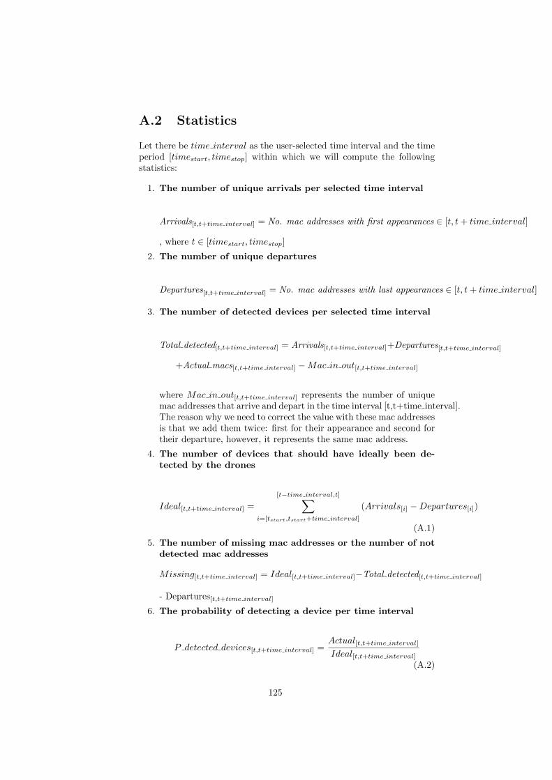
A.2 Statistics

Let there be time interval as the user-selected time interval and the timeperiod [timestart, timestop] within which we will compute the followingstatistics:

1. The number of unique arrivals per selected time interval

Arrivals[t,t+time interval] = No. mac addresses with first appearances ∈ [t, t+ time interval]

, where t ∈ [timestart, timestop]

2. The number of unique departures

Departures[t,t+time interval] = No. mac addresses with last appearances ∈ [t, t+ time interval]

3. The number of detected devices per selected time interval

Total detected[t,t+time interval] = Arrivals[t,t+time interval]+Departures[t,t+time interval]

+Actual macs[t,t+time interval] −Mac in out[t,t+time interval]

where Mac in out[t,t+time interval] represents the number of uniquemac addresses that arrive and depart in the time interval [t,t+time interval].The reason why we need to correct the value with these mac addressesis that we add them twice: first for their appearance and second fortheir departure, however, it represents the same mac address.

4. The number of devices that should have ideally been de-tected by the drones

Ideal[t,t+time interval] =

[t−time interval,t]∑i=[tstart,tstart+time interval]

(Arrivals[i] −Departures[i])

(A.1)

5. The number of missing mac addresses or the number of notdetected mac addresses

Missing[t,t+time interval] = Ideal[t,t+time interval]−Total detected[t,t+time interval]

- Departures[t,t+time interval]

6. The probability of detecting a device per time interval

P detected devices[t,t+time interval] =Actual[t,t+time interval]

Ideal[t,t+time interval](A.2)

125

, where

Actual[t,t+time interval] = Total detected[t,t+time interval]−Arrivals[t,t+time interval]−Departures[t,t+time interval] +Mac in out[t,t+time interval](A.3)

and represent the mac addresses which arrived in a previous interval,but have not departed yet.

7. The corrected percentage of detecting a device per timeinterval

P detected devices[t,t+time interval] =Actual[t,t+time interval]

Corrected Ideal[t,t+time interval](A.4)

where Actual[t,t+time interval] has the same formula previously men-tioned, while the

Corrected Ideal[t,t+time interval] = Ideal[t,t+time interval]−Correction[t,t+time interval]

(A.5), which represents a correction that we use in order to not underes-timate the value of the percentage of devices detected.

8. The average time difference between two consecutive detec-tions

This is computed in two steps. First, we calculate the average deltatime per mac address:

Average delta time maci =

[timestop−time interval,timestop]∑j=[timestart,timestart+time interval]

∆timeij∑[timestop−time interval,timestop]

i=[timestart,timestart+time interval]# detectionsi−1(A.6)

Then we calcu-

late the average delta:

Average deltai =

m∑i=0

Average

∆time macim(A.7)

where m represents the number of unique mac addresses.

The average number of detected devices∑[timestop−time interval,timestop]j=[timestart,timestart+time interval]

# detectionsj

nj(A.8)

, where n represents the number of unique mac addresses detected for each j.

The pull distributionThe pull distribution has the following formula:

pullx(i) =(xi − actualx(i))

σx(i)

pully(i) =(yi − actualy(i))

σy(i)

where the x(i) and y(i) represent the determined coordinates, the actualx(i)and actualy(i) are the actual measurements of a mac address, and the σx(i)and σy(i) are the errors of the algorithms.

126

A.3 Experiments

A.3.1 Experiment 1

A.3.1.1 Test 1

Time Action Other

14:55 Started the experiment Direction towards Foxtrot and Delta15:57 Pressed the home button -15:58 Pressed the home button twice14:59 Pressed the home button -15:01 Pressed the home button -15:02 Pressed the home button -15:04 Pressed the home button -15:05 Pressed the home button the cell phone a bit shifted to the side15:07 Pressed the home button now it has the correct position15:08 Pressed the home button -15:09 Pressed the home button -15:10 Pressed the home button -15:11 Pressed the home button -15:13 Pressed the home button -15:14 Pressed the home button Stop the experiment

Table A.1: Experiment 1 Test 1

A.3.1.2 Test 2

Time Action Other

15:14 Started the experiment Direction towards Echo and Delta15:16 Pressed the home button -15:18 Pressed the home button twice15:19 Pressed the home button -15:21 Pressed the home button -15:22 Pressed the home button -15:23 Pressed the home button -15:26 Pressed the home button twice15:27 Pressed the home button -15:29 Pressed the home button Stop the experiment


A.3.1.3 Test 3

127

Time Action Other

15:30 Started the experiment Direction towards Echo and Charlie15:32 Pressed the home button -15:33 Pressed the home button -15:34 Pressed the home button -15:36 Pressed the home button -15:37 Pressed the home button -15:38 Pressed the home button -15:39 Pressed the home button -15:40 Pressed the home button -15:42 Pressed the home button -15:44 Pressed the home button Stop the experiment


A.3.1.4 Test 4

Time Action Other

15:45 Started the experiment Direction towards Charlie and Foxtrot15:46 Pressed the home button Changed a bit its position15:47 Pressed the home button -15:49 Pressed the home button -15:51 Pressed the home button third times pressed15:52 Pressed the home button -15:54 Pressed the home button twice15:55 Pressed the home button Stop the experiment


A.3.2 Experiment 2

Test Timestart TimeendTest1 13:40 13:49Test2 13:50 14:00Test3 14:03 14:13

Table A.5: Experiment 2

128

A.3.3 Experiment 3

Test HTC IphoneTimestart Timeend Timestart Timeend

Test1 11:40 11:56 15:00 15:16Test2 11:58 12:14 15:19 15:35Test3 12:20 12:36 15:40 15:56Test4 12:38 12:54 15:59 16:15

Table A.6: Experiment 2

A.4 Datasets

The used datasets depend on the experiment and the analyses that were per-formed. For simplicity, these datasets are explained by chapter as follows:

• Chapter 2, Comparison between the two developed algorithms

– The Fitter dataset of the CHEP conference

– The Trilaterator dataset of the CHEP conference

• Chapter 3, Modeling the time dependency of detecting WiFi devices

– The Fitter dataset of the CHEP conference

• Chapter 4, Controlled table top experiments

– Experiment 1

∗ The dataset with the recorded signal strength for the iPhone mo-bile device

∗ The Fitter datasets of the reconstructed points for this experimentbefore the bug fix

– Experiment 2

∗ The dataset with the recorded signal strength for the HTC mobiledevice

– Experiment 3

∗ The dataset with the recorded signal strength for the iPhone andHTC mobile devices

∗ The Fitter datasets of the reconstructed points for the iPhone andHTC before the bug fix

– Experiment 4


∗ The Fitter datasets of the reconstructed points for the iPhone andHTC before the bug fix

• Chapter 5, The performance of the Fitter algorithm

– Experiment 1

∗ The dataset with the recorded signal strength for the iPhone mo-bile device

129


∗ The Fitter datasets of the reconstructed points for this experimentafter the bug fix

– Experiment 3




– Experiment 4

∗ The dataset with the recorded signal strength for the iPhone andHTC mobile device



A.5 Experiments and tests

A.5.1 Experiment 1

A.5.1.1 Test 2

The second test is shown in Figure 4.1b. In this experiment, the cell-phone ison the table turned to the Echo and Delta drones. The start time of the Test2 was at 15 : 13 until 15 : 29. The history of the actions that were performedduring this test can be read in Table A.2.

As in the case of the previous test, we plotted the signal strength distributionover time and per drone. The results are visualized in FiguresA.1 and A.2. Itcan be observed that over time in this case the Foxtrot drone has the highestdetected signal, followed by Delta, Echo, Charlie, and in the end Alpha, which isdifferent from the previous case. In addition to this, Foxtrot has again a smallernumber of records than the rest of the drones.

130

Figure A.1: The signal strength of the five drones during Test 2

From a signal strength distribution perspective, it can be observed that allthe drones seem to have a Gaussian distribution shape. In contrast with Test 1,the highest average value of the signal strength can be found in the case of theFoxtrot drone, followed by the Delta drone with an average value of −48.6±2.1,then by Echo −55.0 ± 5.2, and lastly Charlie −55.9 ± 5.2. These results mayindicate that there is a difference between the signal strengths given the positionof the cell-phone.

Figure A.2: The distribution of signal strength for each of the five drones duringTest 2

131

By looking at the scatter plot in Figure A.3, it can be observed that most ofthe points are still on the table, where they form two clusters. It can observedthat the cluster on the left resembles the one obtained in Test 1, with the xcoordinates shifted to the left side and the y coordinates very close to 0. Besidesthis cluster, one can also see another one on the right side. These points area bit shifted for both coordinates. An explanation for this result may be thatthe Fitter allocates different weights to the received signal strength by differentdrones depending on the magnitude of them. As seen in the previous plots, theFoxtrot drone seemed to detect the most powerful signal strength.

Figure A.3: The determined coordinates by the Fitter algorithm after Test 2

A.5.1.2 Test 3

The third test can visualized in Figure 4.1c. The cell-phone is on the tableturned to the Echo and Charlie drones and the history of the actions that wereperformed in this test is in Table A.3. This third test started at 15 : 30 until15 : 45. As it can be seen in Figure A.4, Foxtrot seems to detect again thehighest signal strength and it seems to have a different shape than the others.By comparing the other drones with each other, Delta seems to have a highersignal than Echo and Charlie, followed in the end by Alpha. According to thisplot, Echo and Charlie detected the same signal at the beginning of this test,but after a while they started differentiating themselves.

132

Figure A.4: The signal strength of the five drones during Test 3

On one hand, when looking at the distribution of the signal strengths inFigure A.5, the shape of Foxtrot’s distribution does not resemble the Gaussianone, which may give us again an indication of the fact that this drone may havesome technical problems. On the other hand, the other drones seem to havethe shape of the normal distribution, with average values in this order: Delta,followed by Echo, Charlie, and in the end Alpha. Compared to the other tests,the Echo and Charlie distributions do not seem to resemble anymore and theyare not centered anymore in a close average signal value. According to Table4.3, the average value of the signal strength for Charlie was −60.3± 3.1 smallerthan the one of Echo −54.2± 2.4.

133


The Fitter algorithm seems to perform less well for this test compared toTest 1 and Test 2, as only 2 points were calculated(Figure A.6). However, thesepoints are detected in the area of the table. As it can be seen, one of the pointsseems to have the y coordinate close to 0, while the other one was detectedin the area of the Foxtrot drone, which can be explained by the fact that thealgorithm allocates a higher weight to the drone which detects the highest signalstrength, which in this case is Foxtrot.

134


A.5.1.3 Test 4

The fourth test is visualized in Figure 4.1d. It started at 15:45 until 15:55. Thecell-phone was placed on the table turned to the Charlie and Foxtrot dronesand the history of the actions that were performed in this test is in Table A.4.According to Figure A.7a, the signal strengths of Charlie, Delta, Echo seem tointersect each other pretty much, especially in the case of Delta and Charlie.This seems to be an interesting aspect, as this result has not occurred before.

135

(a) The signal strength of the five drones during Test 4

(b) The distribution of signal strength for each of the five dronesduring Test 4

Figure A.7: The results of Test 4 experiment 1

When looking at the distributions of the signal strength, it appears thatall the distributions except for Foxtrot seem to follow a Gaussian distribution.Charlie, Delta, and Echo seem to have these distributions centered in prettysimilar average signal strength, which are −52.6 ± 6.0 for Charlie, −49.0 ± 2.1for Delta, and −51.3± 4.3 for Echo(Table 4.3).

136


The scatter plot of Test 4 in Figure A.9 shows that the Fitter algorithmdetects the coordinates of the iPhone close to its actual point. Most of theresulting points form two different clusters on the table, which have the valueof the x coordinate on average close to zero. However, there can be also seenpoints which are positioned outside the table, but still in the room.


137

A.5.2 Experiment 2

A.5.2.1 Measurements of the signal strength versus distance-Test 1

Compared to Test 2 and Test 3, Test 1 has fewer measurements performed andit has detections only up to the 27th meter step. The plot of the measurementfor this test can be visualized in Figure A.10.



Figure A.10: Measurements of Test 1 from experiment 2

The plots of the measurements of both dronesA.10a and A.10b contain not

138

only the measurements, but also the average of these measurements at every 3meter step. It can be seen that the greater the distance is from the drones, thelower the signal strength is.

Due to the fact that the drones are placed next to each other, we expect thatthe signal strength to be detected in the same way, which can be actually seen.However, for the 15th meter step the situation is different, as Charlie detects ahigher signal than Echo. A reason for this situation may be the shape of thehallway, which at the 15th meter step has the entrance of the open-space area,where the desks are located on the left side, while on the right side there arethe rooms of other offices and this may attenuate the signal strength.


By looking at the measurements performed in Test 2 with the results in FigureA.11a and Figure A.11b, it can be seen again that the signal strength decreasesthe further a cell-phone device is, but this is not the case all the time. If theCharlie and Echo measurements are compared with each other, the shape oftheir measurements resembles, except for the 3 meter distance. In addition tothis, the average value of the measurements decreases up to the 9 meters distanceand then it starts increasing in both cases at the 12 meter distance. Then, onone hand, in case of the Charlie drone the average continues to decrease upto 27 meters and then it increases for the 30 meters. On the other hand, thissituation does not actually happen for the Echo drone, where the average signalstrength increases at the 18 meter distance, followed by another increase butless intense at 27 meters. This seems surprising as we would expect the powerof the signal to decrease continuously. One possible reason for this may be theshape of the hallway, the walls, and the metal drawers which may attenuate ormay increase the signal strength at different locations.

139





The measurements of test 3 can be visualized in Figure A.12a and Figure A.12b.Compared to the other experiments, these measurements seem to have in mostcases a smoother decrease even though this is not always the case. It can beobserved that Charlie has again spikes of the average signal strength at 12, 24,and 30 meters distance, while Echo has an average signal spikes at 9, 18, 27, and30. The reason why these spikes occur may be due to the shape of the hallway.

140




A.5.2.4 Chi-square minimization of the average signal strength test1

As it can be seen in Tables 4.5 and 4.6 in the case of Test 1, the curve fitfunction found in the scimpy.optimize Python package did not manage to findthe optimal parameters and instead it returned the initial guesses for severaltrials. Due to this situation, we decided to try the average value of the parameterestimates obtained by applying the same function for Test 2 and Test 3. Thus,

141

in Figure A.13a and Figure A.13b, the calculated function is plotted, which hasthe following form:

f(distance) = −44.9− 0.78× 20× log10 distance

versus the average signal strength obtained from the taken measurements.As it can be seen in Figure A.13a, the fit seems pretty good up to the 12 meterdistance. However, in the interval between 12 up to 18 meters, the calculatedfunction does not entirely fit the data. As mentioned before, it may be thesituation that the shape of the hallway must have influenced the signal strength.However, this is not the same situation for the Echo drone. According to FigureA.13b, the calculated function, which has the following form :


seems to fit pretty well the average values of the signal strength. Given thefact that the curve fit function did not return any optimal parameters for thisdata either, because the function may not have converged, these average valuesof the optimal parameters seem to be quite good, but they may not be the oneswhere the errors are minimized.

142




A.5.2.5 Chi-square minimization of the average signal strength test3

The Figure A.14a and Figure A.14b describe the behavior of the drones Charlieand Echo, respectively in Test 3. The functions are the following:


for the Charlie drone and

143


for the Echo drone.By looking at the first drone, it can be observed that the determined function

with the optimal parameters seems to fit the data better than in the previoustests. The same thing seems to be for the Echo drone, even though it can beseen that the function fits instead the lower bound of the average signal strengthat the 9 meter distance.




144

A.5.3 Experiment 3

A.5.3.1 Test 2

The distributions of the signal strengths can be visualized in Figure A.15a andA.15b. On one hand, as seen in Test 1, the highest average signal strength canbe also seen for Delta for both devices. Apparently, this time the iPhone seemsto detect an higher average than the HTC for Delta drone. In addition to this,the iPhone seems to communicate more with the drones than the HTC whenstreaming data. On the other hand, the Beta drone has the lowest average signalstrength in both cases with −59.9±0.9dBm for the HTC versus −51.4±1.7dBm,respectively for the iPhone. The main difference between the two devices is thatthe HTC is recorded on average better by Echo than Charlie in contrast to theiPhone, which is detected better by Charlie and less by Echo.

145



Figure A.15: The distributions of the signal strength of Test 3 from experiment2

The results of test 2 are not as encouraging as the ones obtained in test 1,because the number of calculated coordinates is small(10 for the HTC and 0for the iPhone) given the high number of sniffed packets. However, a positiveaspect may be that in the HTC case, these points are clustered and the mobiledevice is still seen in the area of the room where the experiment was performed.The values of the average x-coordinate are still pretty small 1.3 ± −0.7 and−0.7± 0.1 for the y coordinate, respectively. These values are higher compared

146

to the ones of the previous experiment.



Figure A.16: The coordinates detected by the Fitter algorithm in case of Test2 from experiment 3

A.5.3.2 Test 3

According to Figures A.15b and A.17b, the Delta drone has again the highestvalues of the average signal strength in the case of both mobile devices. More-over, in the case of the iPhone mobile device, the second highest average signalstrength is followed by the Beta drone, then by the Echo drone, and finally byCharlie. This is not the case with the HTC, which is followed by Echo, Char-lie, and Beta lastly. Besides this, the distributions of Beta, Charlie, and Echooverlap.

147




According to table4.9, the number of calculated points by the Fitter algo-rithm is 25 for the HTC and 2 for the iPhone. This result is comparative to theprevious test, as the algorithm could not compute the position of the iPhonedevice more than twice, but these points were still situated on the table. How-ever, an interesting outcome was again that the determined points were locatedclose to the Delta drone for the HTC case.

The average coordinates obtained by the algorithm in the HTC case were

148

0.9 ± 0.1 for the x-coordinate and −0.7 ± 0.2 for the y-coordinate, while, inthe iPhone’s case, they were 0.4 ± 0.4 for the x-coordinate 0.1 ± 0.3 for the ycoordinate, respectively.




A.5.3.3 Test 4

In the last performed test, it can be seen in Figure A.19a that the distributionsof Beta, Charlie, and Delta overlap. However, Echo seems to be shifted to theleft side and has the smallest average detected signal strength compared to therest. The same situation happens for the iPhone where the distributions ofBeta, Charlie, and Echo overlap, which is in contrast to the HTC case, wherethe distribution of Delta is shifted to the right side and has a higher signalstrength compared to the other ones.

149




According to Figures A.20a and A.20b, it can be clearly seen that test 4represents by far one of the best results obtained from this experiment as thenumber of detected points is 63(HTC) and 63(iPhone). Each test was performedfor 16 minutes. Normally, at every 10 seconds, the Fitter algorithm should pro-vide at least one point. This would mean that for these 16 minute experiments

around (16×6)10 = 96 points should be determined. This means that the algorithm

performed unexpectedly well in the iPhone case.

150

On the other hand, the average coordinates in the HTC case are −0.1± 0.3and −0.6± 0.2 versus the ones calculated for the iPhone with an average for xequal to 0.3± 0.0 and −0.9± 0.1 for y, respectively.




A.6 The performance of the Fitter algorithm -Experiment 1

A.6.1 Test 2

In Test 2, we remind the reader that the position of the iPhone mobile devicewas located with the home button towards the Charlie and Foxtrot routers.According to Table 5.1, the number of calculated points by the algorithm is

151

39, which is much less compared to the previous test. Thus, there were 49time intervals of 10 without no detections and no pattern drawn from theirnon-detections. However, after the bug fix, this issue was remedied and allthe time intervals with packets had points computed. For this experiment, 2time intervals seem to not have any calculated points for the entire experiment.Therefore, the probability of calculating points by the algorithm is equal to 1,as in all the cases where packets were available it computed them.

Figure A.21 shows a nice shape in the number of packets over time. Themajority seem to be more than 5 packets per time interval of 10 seconds. Thisis reassuring, because this experiment was performed mainly by pressing thehome button once a minute. This may indicate that even though the transitionbetween idle to active state is performed, the mobile devices still send sufficientpackets which can be used for applying the trilateration technique.

When looking at the plots of the coordinates Figure A.22, the calculatedpoints by the algorithms can be visualized before the bug fix and after. Asseen in the previous test, the number of points has definitely increased, butthe performance of the resolution did not. In Figure A.22b, the points arescattered in all directions, even though most of them are located on the rightside of the reference point. One of the possible explanations for this result maybe that the routers that seem to record a higher signal strength compared tothe others are Foxtrot and Delta. Compared to Figure A.22a, Figure A.22bcontains much more outliers, which are especially located in outside the area ofthe table and some of them even outside the area of the room. This appearanceof new points affected as mentioned before the average values of x and y. Forexample, the average value of the x coordinate was 0.4± 1 while after the bugfix it became −1.3 ± 2 which represents a significant difference. In addition tothis, the average y coordinate was initially −0.1± 0.7 and later was −1.2± 3.7.Thus, not only the average values of both coordinates are further away from 0,but their uncertainties have increased significantly.

152

(a) The comparison between the states and data packets experiment1 Test 2(before)

(b) The comparison between data records and packets experiment 1Test 2(after)

Figure A.21: The comparison between data records and packets experiment 1Test 2(before and after)

153

(a) The calculated coordinates by the Fitter algorithm experiment 1Test 2(before)

(b) The calculated coordinates by the Fitter algorithm experiment 1Test 2(after)

Figure A.22: The calculated coordinates by the Fitter algorithm experiment 1Test 2(before and after)

A.6.2 Test 3

In Test 3, the position of the mobile device with the home button towards theFoxtrot and Delta routers. One would expect that the routers that would detectthe highest signals strengths would be Charlie and Echo. This is not entirely trueas the Foxtrot and Delta seem to again dominate in having the largest recordedsignal strengths. Another particularity for this test was that the algorithminitially computed only 2 points, which did not make any sense as there were

154

sufficient number of packets for every 10 second time intervals. Thus, accordingto Table 5.1, there were 81 time intervals of 10 seconds with no detections. Inaddition to this, the percentage of time intervals that had detections is 2.4%±5.8%, which is low given the 97.6%±5.8% efficiency of the WiFi tracking system,as there were 2 time intervals with no received packets. However, after thebug fix the algorithm computed points for all the time intervals and the totalefficiency increased significantly from 2.4%± 5.8% to 97.6%± 5.8%.

According to the plots of the coordinates in Figures A.24a and A.24b1 , itcan be seen a significant difference between the two of them, as an increasednumber of points are plotted after the correction of the algorithm. All thesepoints seem to be located as in Test 2 on the right side of the reference point.The majority of points are close to the Foxtrot and Delta routers, which hadthe highest signal strengths. This may reveal again that the orientation of thedevice has an impact on the signal strength which significantly influences thepoints calculated by the algorithm. Thus, by correcting the signal strength theperformance of the points may be improved. This represents a reassuring resultas correcting the signal strength can be controlled, but the position of the mobiledevice cannot.

As mentioned in other tests as well, even though the number of points in-creased significantly, the performance has decreased. For example after the bugfix, the average x coordinate was 71.6±50.4, while the average y coordinate was−5.1± 41.1. Thus, a search into the dataset of the coordinates was performedwhich revealed the existance of 3 computed points with very high x and y coor-dinates, which have a small probability of appearance. However, this situationmay provide evidence that further corrections should be made to the algorithmsuch that these high values are avoided from analyses.

1It may be the case that the plot of the states and packets after the bug fix(Figure A.23b)does not reveal the second time gap. This may happen, because the matplotlib package forpython sometimes does not show the gaps due to the multitude of 10 second time intervals.Thus, it shrinks the image and some time intervals overlap with each other.

155


(b) The comparison between the states and data packets experiment1 Test 3(after)

Figure A.23: The comparison between the states and data packets experiment1 Test 3(before and after)

156




A.6.3 Test 4

The fourth test of experiment 1 was with the home button positioned towardsthe Echo and Delta routers. When looking at the Figures A.25a and A.25b, itcan be seen that on average there are 5 packets per 10 second time intervals,except for one time interval which does not contain any data packets. Thus,the efficiency of the WiFi tracking system is 98.3%± 5.8%. This is a significantresult as this experiment tested the communication with the probe packets.

157

Initially, for this test only 20 points were detected, but afterwards the algorithmcomputed 39 more points which represented all the number of 10 second timeintervals with packets, but no calculated points.

When looking at the Figure A.26, it can be seen again that the newly com-puted points do not improve the accuracy of the detections, as most of them areoutliers are located either in the area of the room or outside the room. Becausethe Foxtrot had on average the highest detected signal strength, the majorityof the points are located close to this router. In addition to this, there are alsopoints scattered on the table, which seem to have the x coordinate close to 0.However, on an aggregated level, the average x coordinate is 0.5 ± 0.8, whilethe y coordinate is 0.7 ± 1.5. Thus, as expected, the resolution of the averagecoordinate did not improve even though there were points computed.

158


(b) The comparison between the states and data packets experiment1 Test 4(after)

Figure A.25: The comparison between the states and data packets experiment1 Test 4(before and after)

159




A.7 The performance of the Fitter algorithm -Experiment 3

A.7.1 Test 2

Test 2 was performed by having the mobile devices with their home buttons ori-ented towards routers Beta and Echo. According the results of test 2(Subsubsection

160

A.5.3.1), the average signal strengths could be found for both devices in the caseof the Delta drone, followed by Echo and Charlie in the HTC case and the re-verse order the iPhone case. In addition to this, this test together with test 3provided initially poor results with respect to the number of points being cal-culated. However, this result changed after the fix and the number of computepoints increased from 10(HTC) and 0(iPhone) to 95 points(Figure A.27 andFigure A.29). In addition to this, the algorithm could not only compute thecoordinates for one time interval for both mobile devices.

A.7.1.1 HTC

An interesting result in the HTC case was that the average x and y coordinatesdid not change even though the number of computed points was significantlyhigher after the bug fix. This was a positive result compared to the one obtainedin experiment 1 where the average x and y changed considerably. For example,according to Table 5.2, the average previous x coordinate was 1.3 ± 0.1, whilethe current one is 1.3±0.1, while for the y coordinate the average was −0.7±0.1compared to −0.8± 0.0.

Figures A.28a and A.28b show the points computed by the algorithm. As itcan be seen in the first figure, there is a small cluster of points located in thevicinity of the Delta router. As mentioned before, the Delta router recordedthe highest signal strength out of the four routers and this may represent one ofthe reasons why the cluster of points is located in that area. A positive aspectis that this cluster of points is still maintained after the bug fix(Figure A.28b),which seem to be concentrated into the same space with a similar shape. Besidesthis, it can be observed that the points are still in the area of the room andclose to the area of the table. This may indicate that if the routers are properlycalibrated the results may improve.

161



Figure A.27: The states and coordinates detected by the Fitter algorithm forthe HTC mobile device in experiment 3 Test 2(before and after)

162

(a) The reconstructed coordinates by the Fitter algorithm for theHTC mobile device experiment 3 Test 2(before)

(b) The reconstructed coordinates by the Fitter algorithm for theHTC mobile device experiment 3 Test 2(after)

Figure A.28: The reconstructed coordinates by the Fitter algorithm for theHTC mobile device experiment 3 Test 2(before and after)

A.7.1.2 iPhone

Test 2 for the iPhone was initially the one which performed the worst. This wasunexpected as there seemed to be a lot of data packets for each 10 second timeinterval. This test was similar to other tests from a number of data packetsperspective, but later contained data points compared to test 2 which did notcompute any data point. However, after the bug fix, for this test 95 datapoints were computed. Due to the absence of data points, there cannot be

163

made any comparison before the initial situation and the current situation froma resolution of coordinates point of view. It can be affirmed that the currentaverage x coordinate is 1.2±2.2 and −1.2±1.0 for the y coordinate, respectively.

In Figure A.30b, a cluster of points can be observed close to the Delta droneand several scattered points are located between the Charlie and the Deltadrones. These points are not on the table, but inside the room. This mayindicate that the signal strength plays a key role in the way the coordinates arereconstructed(Subsubsection A.5.3.1).

164



Figure A.29: The states and coordinates detected by the Fitter algorithm forthe iPhone mobile device in experiment 3 Test 2(before and after)

165

(a) The reconstructed coordinates by the Fitter algorithm for theiPhone mobile device experiment 3 Test 2(before)

(b) The reconstructed coordinates by the Fitter algorithm for theiPhone mobile device experiment 3 Test 2(after)

Figure A.30: The reconstructed coordinates by the Fitter algorithm for theiPhone mobile device experiment 3 Test 2(before and after)

A.7.2 Test 3

Besides Test 2, Test 3 also seemed to have a poor performance initially for bothmobile devices, actually the iPhone performed worse from a number detecteddata points) However, this situation changed when the algorithm was fixed andthe number of points computed for the iPhone was 95 compared to 94 in theHTC case which had one time interval for which the algorithm could not providea solution even though the number of packets was different than 0. In Tables 5.2

166

and 5.3, the average x and y coordinates can be visualized. As it can be seen,the average coordinates in the HTC case did not seem to increase significantly,compared to the iPhone case where the x coordinate increased slightly from0.4±0.4 to 1.0±0.2 and 0.1±0.3 to −0.9±0.3 for the y coordinate, respectively.

A.7.2.1 HTC

The plots of the coordinates can be observed in Figure A.32 where there is aformed cluster of points which is situated close to the Delta router. This clusteris split between the area of the table and the area of the room. Between theFigure A.32a and Figure A.32b, there seems to be a difference only from anumber of computed points perspective. This is also supported by the fact thatthe average x and y coordinates changed slightly from the previous dataset tothe new obtained one after the algorithm was fixed. As mentioned before, theposition of the cluster may be influenced by the signal strengths of the Deltaand Echo routers.

167



Figure A.31: The states and coordinates detected by the Fitter algorithm forthe HTC mobile device experiment 3 Test 3(before and after)

168




A.7.2.2 iPhone

The number of computed points for this test was significantly increased from 2to 95 which meant that the probability that the algorithm determined pointsraised from 2.1%± 5.8% to 99.0%± 3.5%(Table 5.3).

The plots of the points computed by the algorithm can be visualized inFigure A.34 where two main clusters of points can be seen. On one hand, thereis the one which is close to the Delta router and which is located at the area

169

of the table. These points seem to have smaller x and y coordinates. On theother hand, there is another area with scattered points that are located insideand outside the area of the room. These points are positioned in the middlebetween the Beta and Echo routers. This result may be explained by the factthat the distributions of the signal strength of the Beta and Echo routers seemto overlap with each other.

170




171




A.7.3 Test 4

Test 4 was performed with the mobile devices having their home button orientedtowards Charlie and Delta routers. From a performance perspective, this testcan be compared with Test 1 which also had sufficient initial points computed.Thus, it can be seen in Tables 5.2 for the HTC and 5.3 for the iPhone that theaverage x and y coordinates did not considerably alter. This seems a positiveaspect in the sense that the algorithm is able to be consistent even though some

172

changes were made to it. From an efficiency point of view, the total efficiencythe tracking system increased from 64.9% ± 16.8% to 96.9% ± 6.1% in case ofthe HTC, but, in the iPhone case, it only changed slightly from 95.9% ± 7.0%to 96.9%± 6.1%.

A.7.3.1 HTC

Test 4 of the HTC revealed that only 63 points were computed initially. How-ever, this represented the best result obtained for this mobile device. After thealgorithm was modified, the final number of computed points was 94 which wasequal to the one obtained for the iPhone. From a coordinates’ perspective, therewas no significant modification compared to the previous results. For example,the initial average x coordinate was equal to −0.1 ± 0.3 and −0.6 ± 0.2 for y,while the new ones are −0.2± 0.3 for x and −0.9± 0.5 for y.

According to Figure A.36, one can see two main areas with points. Oneof them seems to have a vertical straight shape slightly positioned to the leftand downward side of the reference point. These points tend to have the xcoordinate close to 0. In addition to this, they are split between the area ofthe table and the area of the room and they are located between Delta andCharlie routers. This may be explained by the fact that the routers with thehighest signal strength were Delta, followed by Charlie, Echo, and Beta whichhad overlapping distributions of the signal strength.

173

(a) The states and coordinates detected by the Fitter algorithm forthe HTC mobile device in experiment 3 Test 4(before)

(b) The states and coordinates detected by the Fitter algorithm forthe HTC mobile device in experiment 3 Test 4(after)

Figure A.35: The states and coordinates detected by the Fitter algorithm forthe HTC mobile device in experiment 3 Test 4(before and after)

174




A.7.3.2 iPhone

This test contained an unexpectedly large number of computed data pointscompared to the rest(93 points). Thus, there only 3 time intervals of 10 secondswhich did not contain a reconstructed data point by the algorithm. For 2 outof these three 3 time intervals, the algorithm after it was repaired it was ableto compute points(Figure A.37). This was an encouraging result

Figure A.38 reveal the plots of the reconstructed points for this mobile de-

175

vice. As expected, the shape of the plot did not change, as only two additionalpoints where added. This shape seems to have a vertical straight form locatedbetween the Charlie and Delta routers and outside the area of the table, whichmay be explained by the overlapping distributions of the Charlie and Deltarouters.




176




177

Bibliography

[1] Fayyad, U., Piatetsky-Shapiro, G., & Smyth, P. (1996). From data mining toknowledge discovery in databases. AI magazine, 17(3), 37.

[2] Shaw, M. J., Subramaniam, C., Tan, G. W., & Welge, M. E. (2001). Knowl-edge management and data mining for marketing. Decision support sys-tems, 31(1), 127-137.

[3] Davenport, T. H., Harris, J. G., De Long, D. W., & Jacobson, A. L. (2001).Data to knowledge to results: building an analytic capability. CaliforniaManagement Review, 43(2), 117-138.

[4] Loraine Charlet, A., & Kumar, D. A. (2012). Market Basket Analysis for aSupermarket based on Frequent Itemset Mining. International Journal ofComputer Science Issues (IJCSI), 9(5).

[5] Rekimoto, J., Miyaki, T., & Ishizawa, T. (2007, September). LifeTag: WiFi-based continuous location logging for life pattern analysis. In LoCA (pp.35-49).

[6] Zhang, Z., Zhou, X., Zhang, W., Zhang, Y., Wang, G., Zhao, B. Y., & Zheng,H. (2011, September). I am the antenna: accurate outdoor AP locationusing smartphones. In Proceedings of the 17th annual international con-ference on Mobile computing and networking (pp. 109-120). ACM.

[7] Jiang, J. A., Tseng, C. L., Lu, F. M., Yang, E. C., Wu, Z. S., Chen, C. P., ...& Liao, C. S. (2008). A GSM-based remote wireless automatic monitoringsystem for field information: A case study for ecological monitoring ofthe oriental fruit fly,Bactrocera dorsalis. Computers and electronics inagriculture, 62(2), 243-259.

[8] Chon, J., & Cha, H. (2011). Lifemap: A smartphone-based context providerfor location-based services. Pervasive Computing, IEEE, 10(2), 58-67.

[9] Montoliu, R., & Gatica-Perez, D. (2010, December). Discovering humanplaces of interest from multimodal mobile phone data. In Proceedings ofthe 9th International Conference on Mobile and Ubiquitous Multimedia(p. 12). ACM.

[10] Varshavsky, A., de Lara, E., Hightower, J., LaMarca, A., & Otsason, V.(2007). GSM indoor localization. Pervasive and Mobile Computing, 3(6),698-720.

[11] Zhao, X., Lau, R. S. M., & Lam, K. (2002). Optimizing the service configu-ration with the least total cost approach. International Journal of ServiceIndustry Management, 13(4), 348-361.

178

[12] Al Nuaimi, K., & Kamel, H. (2011, April). A survey of indoor positioningsystems and algorithms. In Innovations in Information Technology (IIT),2011 International Conference on (pp. 185-190). IEEE.

[13] Zeimpekis, V., Giaglis, G. M., & Lekakos, G. (2002). A taxonomy of in-door and outdoor positioning techniques for mobile location services. ACMSIGecom Exchanges, 3(4), 19-27.

[14] Woodman, O., & Harle, R. (2008, September). Pedestrian localisation forindoor environments. In Proceedings of the 10th international conferenceon Ubiquitous computing (pp. 114-123). ACM.

[15] Boztug, Y., & Reutterer, T. (2008). A combined approach for segment-specific market basket analysis. European Journal of Operational Re-search, 187(1), 294-312.

[16] Shaw, M. J., Subramaniam, C., Tan, G. W., & Welge, M. E. (2001). Knowl-edge management and data mining for marketing. Decision support sys-tems, 31(1), 127-137.

[17] http://en.wikipedia.org/wiki/Friis_transmission_equation

[18] A. LaMarca et al.(2005). Place Lab: Device Positioning Using Radio Bea-cons in the Wild. Proc. 3rd Int’l Conf. Pervasive Computing, LNCS 3468,Springer, pp. 116–133.

[19] Prasithsangaree, P., Krishnamurthy, P., & Chrysanthis, P. K. (2002, Septem-ber). On indoor position location with wireless LANs. In Personal, Indoorand Mobile Radio Communications, 2002. The 13th IEEE InternationalSymposium on (Vol. 2, pp. 720-724). IEEE.

[20] Bahl, P., & Padmanabhan, V. N. (2000). RADAR: An in-building RF-baseduser location and tracking system. In INFOCOM 2000. Nineteenth AnnualJoint Conference of the IEEE Computer and Communications Societies.Proceedings. IEEE (Vol. 2, pp. 775-784). Ieee.

[21] Hightower, J., & Borriello, G. (2001). A survey and taxonomy of locationsystems for ubiquitous computing. IEEE computer, 34(8), 57-66.

[22] Cornelius, C., Kapadia, A., Kotz, D., Peebles, D., Shin, M., & Triandopou-los, N. (2008, June). Anonysense: privacy-aware people-centric sensing.In Proceedings of the 6th international conference on Mobile systems,applications, and services (pp. 211-224). ACM.

[23] Kapadia, A., Kotz, D., & Triandopoulos, N. (2009, January). Opportunisticsensing: Security challenges for the new paradigm. In CommunicationSystems and Networks and Workshops, 2009. COMSNETS 2009. FirstInternational (pp. 1-10). IEEE.

[24] Consolvo, S., Smith, I. E., Matthews, T., LaMarca, A., Tabert, J., &Powledge, P. (2005, April). Location disclosure to social relations: why,when, & what people want to share. In Proceedings of the SIGCHI con-ference on Human factors in computing systems (pp. 81-90). ACM.

[25] Harris, L., & Westin, A. F. (2003). Consumer Privacy Attitudes: A MajorShift Since 2000 and Why.

[26] Sadeh, N., Hong, J., Cranor, L., Fette, I., Kelley, P., Prabaker, M., & Rao, J.(2009). Understanding and capturing people’s privacy policies in a mobilesocial networking application. Personal and Ubiquitous Computing, 13(6),401-412.

179

http://en.wikipedia.org/wiki/Friis_transmission_equation

[27] http://www.polestar.eu/en/

[28] http://www.forbes.com/sites/kashmirhill/2014/06/20/

why-a-san-francisco-coffee-shop-stopped-tracking-customers-phones/

[29] http://euclidanalytics.com/

[30] http://www.purplewifi.net/

[31] http://retailnext.net/

[32] http://www.infsoft.com/

[33] Conway, J., Pseudoexperiments,Pulls,and Kinematic Fitting, Physics 252C -Lecture 15.

[34] Mautz, R. (2012). Indoor positioning technologies (Doctoral dissertation, Ha-bil. ETH Zurich, 2012).

[35] JCGM 200:2008: International Vocabulary of Metrology Basic and GeneralConcepts and Associated Terms, 3rd Edition, Joint Committee for Guidesin Metrology.

[36] Thomas, F., & Ros, L. (2005). Revisiting trilateration for robot localization.Robotics, IEEE Transactions on, 21(1), 93-101.

[37] http://en.wikipedia.org/wiki/Trilateration (March 20th 2014)

[38] Demortier, L., & Lyons, L. (2002). Everything you always wanted to knowabout pulls. CDF note, 43.

[39] Chon, Y., Talipov, E., Shin, H., & Cha, H. (2011, November). Mobilityprediction-based smartphone energy optimization for everyday locationmonitoring. In Proceedings of the 9th ACM conference on embedded net-worked sensor systems (pp. 82-95). ACM.

[40] Koyuncu, H., & Yang, S. H. (2010). A survey of indoor positioning and objectlocating systems. IJCSNS International Journal of Computer Science andNetwork Security, 10(5), 121-128.

[41] http://en.wikipedia.org/wiki/Root-mean-square_deviation

[42] Want, R., Hopper, A., Falcao, V.,& Gibbons, J. (1992). The active badge lo-cation system. ACM Transactions on Information Systems (TOIS), 10(1),91-102.

[43] Sayed, A. H., Tarighat, A., & Khajehnouri, N. (2005). Network-based wirelesslocation: challenges faced in developing techniques for accurate wirelesslocation information. Signal Processing Magazine, IEEE, 22(4), 24-40.

[44] Pahlavan, K., Li, X., & Makela, J. P. (2002). Indoor geolocation science andtechnology. Communications Magazine, IEEE, 40(2), 112-118.

[45] Gu, Y., Lo, A., & Niemegeers, I. (2009). A survey of indoor positioning sys-tems for wireless personal networks. Communications Surveys & Tutorials,IEEE, 11(1), 13-32.

[46] Press, William H.; Teukolsky, Saul A.; Vetterling, William T.; Flannery,Brian P. (2007). ”Preface to the Third Edition”. Numerical Recipes: TheArt of Scientific Computing (2rd ed.). New York: Cambridge UniversityPress. p. xi.

[47] Stites D., Skinner K., User privacy on iOS and OS X

180

http://www.polestar.eu/en/

http://www.forbes.com/sites/kashmirhill/2014/06/20/why-a-san-francisco-coffee-shop-stopped-tracking-customers-phones/

http://www.forbes.com/sites/kashmirhill/2014/06/20/why-a-san-francisco-coffee-shop-stopped-tracking-customers-phones/

http://euclidanalytics.com/

http://www.purplewifi.net/

http://retailnext.net/

http://www.infsoft.com/

http://en.wikipedia.org/wiki/Root-mean-square_deviation

[48] http://www.techtimes.com/articles/8233/20140612/

apple-implements-random-mac-address-on-ios-8-goodbye-marketers.

htm

[49] http://www.tomsguide.com/us/ios-8-mac-address-randomization,

news-18937.html

[50] http://www.washingtonpost.com/blogs/the-switch/wp/2014/06/09/

how-apples-new-software-makes-it-harder-for-retailers-to-track-your-movements/

[51] http://thenextweb.com/apple/2013/03/26/

what-exactly-wifislam-is-and-why-apple-acquired-it/

[52] http://www.pcmag.com/article2/0,2817,2416988,00.asp

[53] http://marketingland.com/apple-killed-location-tracking-ios-8-86908

[54] https://angel.co/wifislam

[55] Amoraal, J. M. (2011). Alignment with Kalman filter fitted tracks and recon-struction of B decay.

[56] http://tweakers.net/nieuws/93547/dixons-mycom-en-icentre-volgen-klanten-door-peilen-wifi-signaal.

html

181

http://www.techtimes.com/articles/8233/20140612/apple-implements-random-mac-address-on-ios-8-goodbye-marketers.htm



http://www.tomsguide.com/us/ios-8-mac-address-randomization,news-18937.html

http://www.tomsguide.com/us/ios-8-mac-address-randomization,news-18937.html

http://www.washingtonpost.com/blogs/the-switch/wp/2014/06/09/how-apples-new-software-makes-it-harder-for-retailers-to-track-your-movements/

http://www.washingtonpost.com/blogs/the-switch/wp/2014/06/09/how-apples-new-software-makes-it-harder-for-retailers-to-track-your-movements/

http://thenextweb.com/apple/2013/03/26/what-exactly-wifislam-is-and-why-apple-acquired-it/

http://thenextweb.com/apple/2013/03/26/what-exactly-wifislam-is-and-why-apple-acquired-it/

http://www.pcmag.com/article2/0,2817,2416988,00.asp

http://marketingland.com/apple-killed-location-tracking-ios-8-86908

https://angel.co/wifislam

http://tweakers.net/nieuws/93547/dixons-mycom-en-icentre-volgen-klanten-door-peilen-wifi-signaal.html

http://tweakers.net/nieuws/93547/dixons-mycom-en-icentre-volgen-klanten-door-peilen-wifi-signaal.html

analyzing the performance of a wifi tracking system · analyzing the performance of a wifi tracking...

Documents