analyzing deformation the left v en tricle of the heart ...cohen/mypapers/bardinetrr2797.… ·...

Analyzing the deformation of the left ventricle ofthe heart with a parametric deformable modelEric BARDINET1, Laurent D. COHEN2, Nicholas AYACHE11 INRIA Sophia Antipolis, 2004 Route des Lucioles, B.P. 9306902 Sophia Antipolis CEDEX, France.2 CEREMADE, U.R.A. CNRS 749, Université Paris IX - DauphinePlace du Marechal de Lattre de Tassigny 75775 Paris CEDEX, France.Email: [email protected] present a new approach to analyze the deformation of the left ventricle of the heart, basedon a parametric model that gives a compact representation of a set of points in a 3D image.We present four di�erent approaches to tracking surfaces in a sequence of 3D cardiac images.Following tracking, we then infer quantitative parameters which are useful for the physician,such as the variation of volume and wall thickness during a cardiac cycle, the ejection fractionor the twist component in the deformation of the ventricle. We explicit the computation of theseparameters using our model. Experimental results are shown in time sequences of two kinds ofmedical images, Nuclear Medicine and X-Ray Computed Tomography (CT).KEYWORDS: Parametric models, Tracking, Motion, Heart left ventricle deformation,Quantitative parameters.1 IntroductionThe analysis of cardiac deformations has given rise to a large amount of research in medical imageunderstanding. Indeed, cardiovascular diseases are the primary cause of mortality in developedcountries. Various imaging techniques [1] allow the acquisition of dynamic sequences of 3D images(3D+T) during a complete cardiac cycle (contraction and dilation). These images are perfectlyadapted to studying the behavior of the cardiac system since they visualize how the heart wall

Analyzing heart deformation - submitted to MEDIA 2deforms. Processing these images opens numerous �elds of applications, like the detection andanalysis of pathologies.Advanced techniques of 3D imagery, like Nuclear Medicine and X-Ray CT, provide ever increas-ing resolution in space and time. Consequently, the data available to the radiologist is becominglarger. However, to establish a reliable and fast diagnosis, the physician needs models that arede�ned by only a small number of characteristic quantities. Our parametric deformable modelallows the representation of a dynamic set of points by a reasonable number of useful parameters,as we shall see below.Since it is characteristic of the good health of the heart, the left ventricle motion and deformationhas been extensively studied by medical image processing groups. Since its creation in 1989, ourgroup has pioneered work in the use of deformable models to extract the left ventricle [5, 17, 6, 8,19, 16, 7, 13]. Other groups have also contributed to the understanding of the complex deformationof the ventricle [4, 31, 3, 30, 36, 29].Over the last decade, many surface reconstruction problems have been formulated as the mini-mization of an energy functional corresponding to a model of the surface. Using deformable modelsand templates, the extraction of a shape is obtained through minimization of an energy composedof an internal regularization term and an external attraction potential (data term), illustrated forexample in [23, 14, 43, 26, 41, 19, 28, 45]. The use of such models is often very e�cient for locatingsurface boundaries of organs and structures, and for the subsequent tracking of these shapes in atime sequence.Although previous approaches based on general deformable surfaces [19, 16] give satisfyingresults, they involve very large linear systems to solve. This is why the parametric model presentedhere is more appropriate when dealing with a huge amount of data as is the case for object trackingin a sequence of 3D images. In a previous article [11], we introduced a parametric deformable modelbased on a superquadric �t followed by a free-form deformation (FFD). In the present article, aftera brief review of the parametric model in section 2, we describe our segmentation algorithm, speci�cto cardiac images, in section 3. Then, in section 4 we present several approaches to track surfaceswith a parametric model in a sequence of 3D images, and give experimental results for trackingthe deformation of the left ventricle in di�erent kinds of 3D medical images. In section 5, weexplain how to infer, from the parametric reconstruction, quantitative parameters which are usefulfor the physician, like the variation of volume and wall thickness during a cardiac cycle, the ejection

Analyzing heart deformation - submitted to MEDIA 3fraction or the twist component in the deformation of the ventricle.2 A parametric model to �t 3D structuresIn this section, we describe brie�y the deformable model that we use to represent the inner andouter walls of the left ventricle.We assume that a segmentation algorithm has already been applied to the 3D images of theheart to extract a number of 3D points belonging to the surface of the inner or outer wall of theleft ventricle (this algorithm is described in section 3).The advantage of parametric deformable templates such as superquadrics or hyperquadrics isthe small number of parameters needed to represent a shape. However, if these models give a goodglobal approximation to a surface, the set of shapes described by superquadrics is too limited toapproximate precisely complex surfaces. To take into account local deformations, Terzopoulos andMetaxas [42] couple superquadrics with a deformable model. In [15], an implicit approach is usedto re�ne the initial approximation.We re�ne our superquadric model using a parametric deformation. More precisely, for a givenset of 3D points, we �rst �t 3D data with a superellipsoid, and then re�ne this crude approximationusing Free Form Deformations (FFDs).2.1 Fitting 3D data with superquadricsSuperquadric shapes have been widely used in Vision and Graphics. In computer vision, their �rstuse is due to Pentland [32], followed by Solina and Bajcsy [9, 37, 38] who used superellipsoidsto approximate 3D objects. The goal of the algorithm is to �nd a set of parameters such thatthe superellipsoid best �ts the set of data points. Superquadrics form a family of implicit surfacesobtained by extension of conventional quadrics. Superellipsoids are de�ned by the implicit equation:0@ � xa1�2=�2 + � ya2�2=�2!�2=�1 + � za3�2=�11A�1=2 = 1: (1)Suppose that the data we want to �t with the superellipsoid are a set of 3D points (xi; yi; zi); i =1; � � � ; N . Since a point on the surface of the superellipsoid satis�es F = 1, where F is the functionde�ned by equation (1), we �nd the minimum of the following energy:E(A) = NXi=1 [1� F (xd; yd; zd; a1; a2; a3; �1; �2)]2 ; (2)

Analyzing heart deformation - submitted to MEDIA 4using a minimization algorithm (see [10] for details and also for a geometric interpretation of thisenergy).2.2 Re�nement with Free Form Deformations (FFDs)We now re�ne this parametric representation of the 3D data, using a global volumetric deformationcalled FFD. This is a tool devoted to the deformation of solid geometric models in a free-formmanner (see [33]). The main interest of FFDs is that the resulting deformation of the object,although potentially complex, is de�ned by a small number of points. This characteristic featureallows us to represent voluminous 3D data by a model de�ned by a small number of parameters.2.2.1 De�nition of FFDsFFDs were introduced by Sederberg and Parry [33] in computer graphics and have been used tosolve matching problems by Szeliski and Lavallée [39, 40]. An FFD is a mapping from IR3 to IR3,de�ned by the tensor product of trivariate Bernstein polynomials. The principle of FFDs is asfollows: the object to be deformed is embedded in a 3D box. Inside this box, a volumetric gridof points is de�ned, which links the box to the object (by the trivariate polynomial which de�nesthe deformation function). This can be written in a matrix form: X = BP , where B is thedeformation matrix ND �NP (ND is the number of points on the discretized superellipsoid andNP is the number of control points of the grid), P is a matrix NP � 3 which contains coordinatesof the control points and X is a matrix ND� 3 with coordinates of the model points. The box isthen deformed by the displacement of its lattice, and the position of a point of the deformed objectis computed (see [11] for details).2.2.2 The inverse problemWe need to solve the inverse problem: �rst compute a displacement �eld �X between the superel-lipsoid and the data, and then, after having put the superellipsoid in a 3D box, search for thedeformation �P of this box which will best minimize the displacement �eld �X :min�P kB�P � �Xk2 (3)This is illustrated in �gure 1.

Analyzing heart deformation - submitted to MEDIA 5

Figure 1: From the superellipsoid to the �nal model. Top left: data. Top right: superellipsoid �t andinitial box of control points. Bottom left: displacement �eld between data and the superellipsoid.Bottom right: �nal model after minimization of the displacement �eld (see [11] for details).

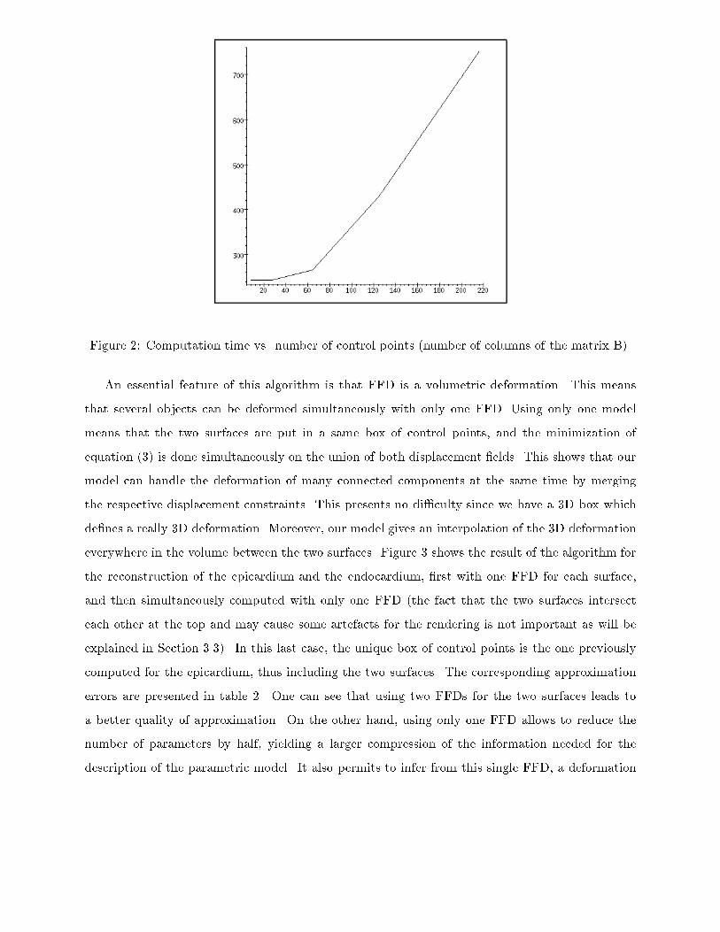
Analyzing heart deformation - submitted to MEDIA 62.2.3 Iterative algorithmTo represent 3D data with our model, we use an iterative two-step algorithm:Step 1 : Computation of the displacement �eld between the previous estimation Xnand its projection on data Xan, �Xn such as: Xan =Xn + �XnStep 2 : Computation of the control points P n+1 by minimization of kBP �Xank2Computation of the deformed model: Xn+1 = BP n+1Stop test on the least-squares error kXn+1�XnkP 0 is de�ned as a uniformly spaced parallelepiped box of control points and X0 = BP 0 representsthe set of points of the initial discretized superellipsoid. This algorithm is similar to the formulationof the B-splines snakes with auxiliary variables, as described in [18].Size of the FFD Computation time2� 2� 2 = 8 2433� 3� 3 = 27 2444� 4� 4 = 64 2655� 5� 5 = 125 4296� 6� 6 = 216 751Table 1: Typical computation times (in seconds) with an increasing number of control points ofthe FFD for 20 iterations.In practice, we use boxes of size 5 � 5 � 5 for data composed of about 6,000 points, and thenumber of iterations is between 10 and 30. Therefore we get a compression rate of 47 (computedas (6000�3)=(125�3+11), where 11 corresponds to the parameters needed for the superellipsoid.In the following, we will write that the model is de�ned by 130 points). Table 1 presents typicalcomputation times of the FFD with 20 iterations and di�erent sizes for the box of control points(on a DEC Alpha 300). One can get a qualitative idea of the algorithmic complexity from �gure 2.2.2.4 Simultaneous deformation of two surfaces


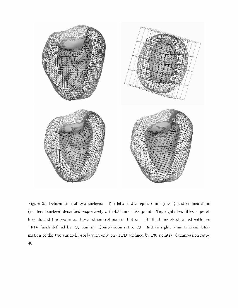
Figure 2: Computation time vs. number of control points (number of columns of the matrix B).An essential feature of this algorithm is that FFD is a volumetric deformation. This meansthat several objects can be deformed simultaneously with only one FFD. Using only one modelmeans that the two surfaces are put in a same box of control points, and the minimization ofequation (3) is done simultaneously on the union of both displacement �elds. This shows that ourmodel can handle the deformation of many connected components at the same time by mergingthe respective displacement constraints. This presents no di�culty since we have a 3D box whichde�nes a really 3D deformation. Moreover, our model gives an interpolation of the 3D deformationeverywhere in the volume between the two surfaces. Figure 3 shows the result of the algorithm forthe reconstruction of the epicardium and the endocardium, �rst with one FFD for each surface,and then simultaneously computed with only one FFD (the fact that the two surfaces intersecteach other at the top and may cause some artefacts for the rendering is not important as will beexplained in Section 3.3). In this last case, the unique box of control points is the one previouslycomputed for the epicardium, thus including the two surfaces. The corresponding approximationerrors are presented in table 2. One can see that using two FFDs for the two surfaces leads toa better quality of approximation. On the other hand, using only one FFD allows to reduce thenumber of parameters by half, yielding a larger compression of the information needed for thedescription of the parametric model. It also permits to infer from this single FFD, a deformation


Figure 3: Deformation of two surfaces. Top left: data: epicardium (mesh) and endocardium(rendered surface) described respectively with 4500 and 1500 points. Top right: two �tted superel-lipsoids and the two initial boxes of control points. Bottom left: �nal models obtained with twoFFDs (each de�ned by 130 points). Compression ratio: 23. Bottom right: simultaneous defor-mation of the two superellipsoids with only one FFD (de�ned by 130 points). Compression ratio:46.

Analyzing heart deformation - submitted to MEDIA 9Separate computation Simultaneous computation Precision lostEpicardium 0.007448 0.008236 10.5 %Endocardium 0.012838 0.014376 11.9 %Table 2: Least-square errors kBP�Xk between original data and parametric models. Left column:each model is computed independently. Middle column: the two models are computed with oneFFD. Right column: computation with only one FFD leads to a slight loss of the approximationprecision.�eld over the entire space, due to the volumetric formulation of FFDs. In the particular caseof cardiac deformations, it allows estimation of the deformation at any point within the volumebetween the epicardium and the endocardium, namely the myocardium. We show in �gure 4 the

Figure 4: Volumetric deformation. FFD previously computed simultaneously from the two isosur-faces (�gure 3) is applied to rigid links between the two superellipsoid models (on the left) andprovides an elastic volumetric deformation of the myocardium (on the right).e�ect of the FFD applied to the volume between the two superellipsoids. To visualize this volumeinformation, we show on the left the segments linking these two surfaces. The FFD computed toobtain simultaneously the epicardium and the endocardium surfaces also deforms these segments.

Analyzing heart deformation - submitted to MEDIA 103 Segmentation of cardiac imagesIn order to get sets of 3D points which correspond to the anatomical structure that we want totrack (epicardium and endocardium of the cardiac left ventricle), and therefore �t our model onthese sets of points, we have to segment the original data.The models were computed on two di�erent kinds of images:� Nuclear medicine data, the SPECT sequence, with 8 successive time frames during one cardiaccycle. Each image is a volume of 64� 64� 64 voxels.� X-Ray CT data, the DSR sequence, with 18 successive time frames during one cycle. Eachimage is a volume of 98� 100 � 110 voxels (size of the voxel: 0.926 mm3).The original 3D images are visualized as a series of 2D cross-sections (transverse slices) in �gures 5and 6. On the DSR data, the ventricular cavity (high grey levels) is clearly shown up but theouter wall of this cavity does not stand out, thus we will use the DSR sequence to analyze thedeformation of the inner wall of the left ventricle (endocardium). On the SPECT sequence, whichis with high contrast, we will study at the same time the deformation of the inner and outer wallsof the left ventricle (endocardium and epicardium). As one can observe from �gures 5 and 6,the extraction of the endocardium on the DSR image is not a very di�cult task, because of thehigh contrast between the endocardium and the rest of the image. Concerning the SPECT images,which are also fairly noisy, a single thresholding will not provide the areas of interest.We �rst recall some properties of SPECT and DSR techniques (sections 3.1 and 3.2) and thendetail our speci�c segmentation algorithm in section 3.3.3.1 Nuclear medicine data (SPECT)Nuclear Medicine provides two types of images: 1. PET (Positron Emission Tomography) and2. SPECT (Single Photon Emission Computed Tomography). These medical imaging modalitiesconstitute the two di�erent modalities of ECT (Emission-Computed Tomography). ECT has beenwidely used in biomedical research and clinical medicine during the last twenty years. ECT dif-fers fundamentaly from many other medical imaging modalities in that it produces a mapping ofphysiological functions as opposed to visualizing anatomical structure. SPECT imaging techniquesemploy radioisotopes which decay emitting a single gamma photon. This represents the fundamen-tal di�erence between SPECT and PET. A typical transaxial resolution in SPECT ranges from


Figure 5: 3D image of the left ventricle - SPECT image (the order of sections reads from left toright and from top to bottom and descends through the heart).10 to 20 mm. Resolution in the axial direction speci�es the slice thickness and is determined bythe collimation properties of the detectors; typically the axial resolution ranges from 10 to 20mm.One can �nd a complete description of the Nuclear Medicine imaging techniques in the tutorialarticle [1].3.2 X-Ray CT data (DSR)The images of this time sequence have a very high resolution (98 � 100 � 110 for a voxel size of0.926 mm3). They were obtained with the Dynamic Spatial Reconstructor (DSR), which is a X-RayCT Scanner capable of providing dynamic synchronous volume 3D CT images, with a time step of1/60 s. X-Ray CT is a medical imaging modality which allows acquisition of a 3D representationof internal anatomical structures. A complete description of X-Ray imaging techniques can also befound in the tutorial article [1]. To get these images, a contrast agent has been injected into theventricle, enhancing the appearance of the cavity.


Figure 6: 3D image of the left ventricle - DSR image (the order of sections reads from left to rightand from top to bottom and descends through the heart).

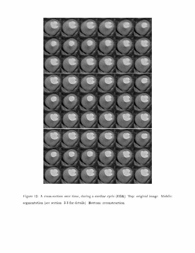
Analyzing heart deformation - submitted to MEDIA 133.3 Morphological segmentationTo obtain an accurate and robust segmentation, we must combine thresholding with mathematicalmorphology and connected components analysis (as in Hoehne [25]). We �rst choose a thresholdwhich grossly separates the ventricle (high values in SPECT and DSR images) from the rest ofthe image. The same value is chosen for the whole sequence of images, which makes the algorithmentirely automatic. Then we choose the largest connected component for each of the resulting 3Dbinary images, and perform a morphological closing of order k (a closing of order k consists in aseries of k dilations followed by the same number of erosions [34, 35]). Typically, this number is equalto 3. This last operation is necessary to bridge small gaps and smooth the overall segmentation.Finally, the extraction of the isosurfaces from this sequence of images provides the set of 3D pointsthat we need as input for the following reconstruction and tracking algorithm. However, it has tobe precised that this set is unstructured. This is why getting a representation as we give is animportant contribution.To understand the complex behavior of the cardiac muscle, we have to recover the deforma-tions of both the internal and external walls of the myocardium, namely the endocardium andthe epicardium. It is possible to represent the geometry of the complete myocardium by a singledeformable superellipsoid-based model. However, by recovering the large concavity which corre-sponds to the ventricular cavity, which means a strong displacement constraint, it follows that allthe other constraints are neglicted, thus involving a smoothing e�ect on the surface model. On theother hand, the shape of the myocardium looks very much like two deformed concentric ellipsoids,and it is thus natural to use two models to recover the two cardiac walls.As we said, the segmentation of the SPECT sequence provides a set of isosurfaces. To get twoseparate closed surfaces of the epicardium and endocardium, we use again morphological operations(closings and logic additions). For this reason, we have arti�cial caps at the base of the heart (ontop of the �gures, for example in �gures 11 and 12). This yields to some slight visual artifacts,because the two surfaces intersect each other at the top, but this e�ect is minor both on the followingcomputation of quantitative parameters (cf. section 5) or for the qualitative analysis which is basedmainly on the observation of the remaining part of the surface.Results of those operations on the dynamic sequence are presented on �gures 11 and 13 (onecross-section over time). For a correct estimation of the quality of those segmentations, we super-imposed the segmented surface on the image.

Analyzing heart deformation - submitted to MEDIA 14Although extracting isosurfaces from the SPECT sequence seems to be a �ddly task, it is madetotally automatic. First, an initial threshold is used to isolate the myocardium. The threshold isset at 40% of the histogram maximum, similarly to the procedure developed by Pr. Michael Gorisat Stanford for the analysis of SPECT images [22]. From this thresholded image, we obtain anisosurface which represents the myocardium. It has two components, as seen on �gure 11. To get thetwo isosurfaces corresponding to the walls of the myocardium, we �rst apply a morphological closingwhich provides the external surface (epicardium), and then, by application of a mask, we erase theexternal surface from the myocardium isosurface and get the internal surface (endocardium).4 Dynamic tracking of the left ventricleHaving extracted 3D points corresponding to the walls of the left ventricle in a time sequence ofimages, we show in this section how we use our parametric model of section 2 to make an e�cienttracking of the LV wall in a sequence of 3D images of di�erent modalities.We present four strategies to use this model to track surfaces in a sequence of 3D images insection 4.1. To make an e�cient comparison between those strategies, we present in this sectionerror measurements and results computed on a synthetic example: a sequence of parametric surfacesrepresenting a synthetic heart during a complete cardiac cycle (17 successive time frames), see�gure 7. All the hearts of this sequence were obtained with the following implicit equation: � xa1�2 + � ya2�2 + � za3�2!3 � c1 � xa1�2 + c2 � ya2�2!� za3�3 = 1;with di�erent values for c1 and c2. Actually, a synthetic example is well suited to compare thetheoritical pros and cons of each strategy, and to choose the most accurate one for the analysis ofcardiac motion.We then present examples on two sequences of 3D medical images in section 4.2. In the followingchapter, we will show how to take advantage of the parametric model to easily compute someimportant quantitative parameters which help to characterize cardiac motion, in particular thevariation of volume and wall thickness during a cardiac cycle, the ejection fraction or the twistcomponent.


Figure 7: Synthetic beating heart (17 successive time frames). From top to bottom and from leftto right: frame 1, 8, 12, 15.

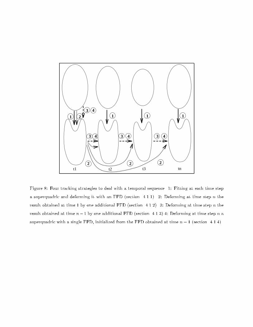
Analyzing heart deformation - submitted to MEDIA 164.1 Four tracking strategiesGenerally deformable models need an initialization which is close enough to the solution. This isconvenient for tracking in medical images since the deformation between two images is small andthe model can start with the solution in the previous image as an initialization for the current one.Deformable contours have been used for tracking boundaries since their introduction by Kass,Witkin and Terzopoulos [43]. This was applied to spatial tracking of the ventricle boundary insuccessive cross-sections of a 3D MR image in [17], in view of 3D reconstruction from a sequenceof 2D models, and later applied to temporal tracking for ultrasound images in [8].With our parametric deformable model, the initialization is made automatically through theinitial superquadric �t (see section 2.1), and then re�ned by the FFD. We studied four di�erentapproaches for tracking which are described in �gure 8 and now brie�y presented. We computedfor each strategy a global error (kBP �Xk), which consists in projecting each 3D data point ontothe deformed model (see �gure 9).4.1.1 Fitting the model independently to each imageThis �rst approach consists in �tting the deformable model independently to each segmented 3Dimage. In this approach, we do not use the continuity of the motion, and the deformation obtainedat time n does not take advantage of the deformation computed at time n � 1. The error curvelabelled 1 in �gure 9 show the global errors between the model and the 3D points of the syntheticsequence. This is clearly the least accurate approach to computing the volumetric properties of theventricle. On the other hand, we do not need any previous model information to de�ne the modelat time n, but only the superellipsoid and the FFD.Following the formulation of section 2.2.3, the model at time n, Xn, can be written:8>>>>>>>>>>>>>>>>>><>>>>>>>>>>>>>>>>>>:Xsq0 = B0P 0X0 = B0 (P 0 + �P �0)Xsq1 = B1P 1X1 = B1 (P 1 + �P �1)...Xsqn = BnP nXn = Bn (P n + �P �n)


1

t2t1 t3 tn

2

3 4

2

3 4

1 1 1

2

3 4 43

2Figure 8: Four tracking strategies to deal with a temporal sequence. 1: Fitting at each time stepa superquadric and deforming it with an FFD (section 4.1.1). 2: Deforming at time step n theresult obtained at time 1 by one additional FFD (section 4.1.2). 3: Deforming at time step n theresult obtained at time n� 1 by one additional FFD (section 4.1.3) 4: Deforming at time step n asuperquadric with a single FFD, initialized from the FFD obtained at time n� 1 (section 4.1.4).


Figure 9: Four tracking strategies (2). Time evolution of the least square error between the data(synthetic sequence, see �gure 7) and the �nal model for the 17 frames. The four curves correspondto the four approaches.

Analyzing heart deformation - submitted to MEDIA 19where P i + �P �i denotes the result of the minimization of kBi P i �Xai k (see section 2.2.3), andXsqi denotes the sequence of initial superellipsoids.4.1.2 Independent representation with a reference deformationA superellipsoid is computed and deformed by a FFD to �t the surfaces extracted in the �rstimage. This then acts as a reference surface which is deformed by only one additional FFD, to �tthe surfaces extracted in image n. The error curve is shown in �gure 9 by the curve labelled (2).The approximation is more accurate, being the composition of two FFDs and each image is nowdescribed with only one set of superellipsoid parameters and two FFDs. This technique is thusindependent of the length of the time sequence. The method is a trade-o� between the techniquesof section (4.1.1) and section (4.1.3).As with the previous method, this approach does not provide temporal processing, but the useof a reference model achieves more accurate solutions.Following the formulation of section 2.2.3, the model at time n, Xn, can be written:8>>>>>>>>>>>>>>>>>>>>><>>>>>>>>>>>>>>>>>>>>>:Xsq0 = B0P 0X0 = B0 (P 0 + �P �0)X0 = B1P 1X1 = B1 (P 1 + �P �1)X1 = B1P 2...Xn�1 = B1P nXn = B1 (P n + �P �n)where P i + �P �i denotes the result of the minimization of kB1 P i �Xai k (see section 2.2.3), andXsq0 denotes the initial superellipsoid at time 0.4.1.3 Recursive representationThis approach is real temporal tracking. The complete model (superquadric �tting and free-form-deformation) is applied only to the data of the �rst image. Then, at time n, the model is obtainedfrom the previous one by deforming the shape obtained at time n�1 by a new FFD. Therefore, thesurface at time n is obtained from the superellipsoid at time 1 iteratively deformed by a sequence ofn successive FFDs. This provides the advantage of being an increasingly accurate approximation,

Analyzing heart deformation - submitted to MEDIA 20but at the expense of a number of parameters increasing linearly with the number of images (themodel at time n is de�ned by n FFDs). The error curve is shown in �gure 9 by the curve labelled(3).Following the formulation of section 2.2.3, the model at time n, Xn, can be written:8>>>>>>>>>>>>>>>>>>>>><>>>>>>>>>>>>>>>>>>>>>:Xsq0 = B0P 0X0 = B0 (P 0 + �P �0)X0 = B1P 1X1 = B1 (P 1 + �P �1)X1 = B2P 2...Xn�1 = BnP nXn = Bn (P n + �P �n)where P i + �P �i denotes the result of the minimization of kBi P i �Xai k.4.1.4 Recursive representation with a unique deformationThis approach is also real temporal tracking. The di�erence with the previous method is that onlyone FFD is needed to compute all the parametric models in the sequence. More precisely, thecomplete model is �tted only to the data of the �rst image. Then, a unique FFD (which is nowa deformed box of control points) is used with a new displacement �eld computed between theprevious model and the data of the next image, and so on for the complete sequence. Finally, themodels at any time are de�ned by only one FFD applied to a single original superellipsoid. Theerror curve is shown in �gure 9 by the curve labelled (4).Following the formulation of section 2.2.3, the model at time n, Xn, can be written:Xn = B0 (P 0 + �P �0 + � � �+ �P �n�1) ; (4)where P i + �P �i denotes the result of the minimization of kB0 P i �Xai k.4.1.5 DiscussionFrom the error curve of �gure 9, one can see that the second method is superior to the �rst oneby reducing and even stabilizing the error values after time frame 2. In addition, methods 3 and4, which provide a real temporal tracking (this is the reason why these curves are decreasing)


Figure 10: Four tracking strategies (4). Temporal evolution of the least square error between thedata and the model during the complete sequence, including each model initialization (peak values)and the following iterations. From left to right and from top to bottom: approaches 1, 2, 3, 4.

Analyzing heart deformation - submitted to MEDIA 22, generate comparable errors along the sequence (the third one gives slightly better results butrequires much more parameters). Figure 10 represents the evolution of the error shown in �gure 9,but with all intermediate iterations. Remark that the error curves of method 4 in �gure 9 is themost regular. Moreover, we can notice that method 4 requires the inversion of a linear system ofthe form X = BP (by computing the pseudoinverse of the matrix with the SVD) only once, andis therefore much faster than the others.For all these reasons, we selected method 4 in the next section to compute the quantitativevolumetric parameters characterizing the deformation of the left ventricle.4.2 Experimental results on cardiac imagesWe present in this section results of the tracking algorithm on the cardiac images described insection 3.Figure 11 shows the dynamic SPECT sequence on a particular cross-section, with the segmentedand reconstructed surfaces superimposed (see section 3.3). It also shows the reconstruction of thesetwo surfaces using either one or two models as explained in section 2.2.4. Figure 12 depicts thesame results for the 3D rendering of the surface.Figure 13 shows the dynamic DSR sequence on a cross-section, �rst the original image, thenthe segmented endocardium surface superimposed (see section 3.3), and also the reconstruction ofthis surface with the parametric model. Figure 14 depicts the same result for the 3D rendering ofthe surface for three time steps of the sequence.FFD Model Iterations Frames Computation timeSPECT 125 2500 10 8 25DSR 125 5000 10 18 72Table 3: Computation times (in minutes) for tracking the complete DSR and SPECT2 sequences(also number of iterations, number of points on the FFD and the models, and number of timeframes).We see from these �gures that the method provides an accurate tracking of the myocardiumwalls, on two di�erent imaging modalities, con�rming visually the quantitative results obtained onthe previous synthetic data. Table 3 shows the CPU time for each complete time sequence (on a


Figure 11: Segmentation and representation of the epicardium and the endocardium (external andinternal walls of the ventricle) for a time sequence (3D+T) of the left ventricle during the cardiaccycle - SPECT image; visualization of a cross-section over time. Top: isosurfaces superimposed onthe image. Middle: reconstruction of the two isosurfaces by two models. Bottom: simultaneousreconstruction of the two surfaces by one model (see Section 3.3 for details).


Figure 12: Time sequence of the epicardium (mesh) and the endocardium (rendered surface) -SPECT image. On the left : isosurfaces obtained by data segmentation (4500 + 1500 points). Onthe right : representation by two parametric models (2� 130 parameters).


Figure 13: A cross-section over time, during a cardiac cycle (DSR). Top: original image. Middle:segmentation (see section 3.3 for details). Bottom: reconstruction.


Figure 14: Time sequence of the endocardium (t= 1; 8; 13). On the left : isosurfaces obtained bydata segmentation de�ned by 10000 points. On the right : reconstruction by the parametric modelde�ned by 130 points (DSR). Compression ratio: 77.

Analyzing heart deformation - submitted to MEDIA 27DEC Alpha 300).5 Quantitative analysis of left ventricle deformationThe reconstruction and representation of a time sequence of surfaces by a sequence of parametricmodels allows to visualize the estimation of the deformation in time. More precisely, the parametricrepresentation provides a way to determine the motion �eld on the cardiac walls. This motion �eldcan then be used to extract some characteristic parameters and give interpretation or diagnosis onthe patient. In the area of cardio-vascular diseases, and especially in the study of cardiac muscle,the useful parameters for diagnosis, as mentioned in the introduction, are primarily the variationof the volume and heart wall thickness during a cardiac cycle, the ejection fraction , and the twistcomponent in the deformation of the ventricle. We explain in this section how we extract thoseparameters from the previously described parametric representation of time sequences of cardiacimages. Similar parameters are also obtained in the work of [30] quantifying the left ventricledeformation.5.1 Volume evolution

ES EDt

V

1 2 3Figure 15: Typical shape of the temporal evolution of ventricular volume. The curve is dividedinto 3 parts: 1. Fast contraction 2. Fast dilation 3. Slow dilation

Analyzing heart deformation - submitted to MEDIA 28To evaluate the ejection fraction, we need a way to compute the temporal evolution of theventricle cavity volume. We �rst show how to calculate the volume of a polyedric region boundedby a mesh of vertices, using the discrete form of the Gauss integral theorem, and then calculate anexplicit form of the volume of a superellipsoid, depending on its parameters.5.1.1 Volume inside a meshLet D be a region of space with bounding surface @D; the unit normal vector n to @D is drawnoutwards. Then: Z Z ZD @u(x; y; z)@x dx dy dz = Z Z@D u cos(n; x) dS (5)(and similarly for y and z). Equation 5 holds under very general assumptions: umust be continuousin D and have continuous bounded �rst partial derivatives; the boundary surface @D must havecontinuously varying tangent planes, except at �nitely many vertices and edges. From this equation,we obtain (among others) the following formula:Z Z ZD div u = Z Z@D u dS = Z Z@D(u; n) dS ;known as the Gauss integral theorem, where div(:) denotes the divergence of a vector �eld and(:; :) denotes the scalar product in IR3.Let O be a reference point. Using this theorem, we can write:Z Z ZD div(OM) dx dy dz = Z Z@D(OM;n) dS;where M is a point on @D. Now, it is obvious that the value of the divergence of the vector �eldOM is 3. Therefore, the Gauss integral thereom yields an expression of the volume inside a domainD: V = Z Z ZD dV = 13 Z Z@D(OM;n) dS (6)Considering an oriented mesh de�ned by a set of points and a set of facets, the volume insidethe mesh can be written, using the previous formula:V = KXi=1 Vi = 13 KXi=1 (OM;N) Si; (7)where K is the number of facets of the mesh.This expression can be rewritten: V = 16 KXi=1 (OG;Nd) ;

Analyzing heart deformation - submitted to MEDIA 29whereNd and G denote respectively the normal vector and the barycentre of a facet (see appendix Afor details of computation).We applied this calculation of epicardium and endocardium volumes to the sequences of bothdata points and parametric models obtained in the previous sections. Once we have the values ofthe volume along a cardiac cycle, we can easily obtain the ejection fraction (calculated preciselyas: Vd� VcVd , with Vd volume at dilation (the end of diastole), V c volume at contraction (the endof systole), see for example [20]. The results presented in �gure 16 show that:� The evolution of the volume has the expected typical shape found in the medical literature[22] and shown in �gure 15. Moreover, the estimation of the ejection fraction on our examplegives a value of 68%, which is in the range of expected values [22, 20].� The volumes computed with all the data points or the approximation models are almost equalas seen from the error curve in �gure 16. The relative average error along the cycle is 0:42%.This proves that our model is robust with respect to the volume estimation. Of course, theejection fraction is also obtained with a very small relative error (0:19%).� The volume evolution found for initial superellipsoid models before FFD, have also a verysimilar shape, as seen in �gure 16. However, there is a size ratio due to the over-estimation ofthe volume before the FFD. This ratio is almost constant in time, which makes it possible toget a good estimate of the ejection fraction directly from the initial model. This proves thatthe superellipsoid model provides a good global estimate of the shape. Also, the volume of thesuperellipsoid can be obtained analytically from its set of parameters without the previousdiscrete approximation (see 5.1.2).5.1.2 Volume of a superellipsoidLet S be a superellipsoid surface de�ned by the following implicit equation:0B@� xa1� 2�2 + � ya2� 2�21CA�2�1 + � za3� 2�1 = 1: (8)Its volume can be explicitly computed by using the following formula:V = 2 a1 a2 a3 �1 �2�(�22 ; �22 + 1) �(�12 ; �1 + 1)See appendix B for details of computation.


Figure 16: Cardiac volumes during the cardiac cycle. Left: volumes of the epicardium (SPECT).Middle: volumes of the endocardium (SPECT). Right: volumes of the endocardium (DSR). Top:volumes of the data. Middle: errors between the volumes of the data and the volumes of themodels. Bottom: volumes of the superellipsoid models. Note that the relative average errors alongthe cycle are less than 1%.

Analyzing heart deformation - submitted to MEDIA 315.2 Wall thickness

Figure 17: One volume element in the volumetric model of the myocardium.Another important feature that is useful for the diagnosis is the evolution of the wall thicknessduring the cardiac contraction. Computing only one model to recover the deformation of both theepicardium and the endocardium permits easy calculation of this parameter. Figure 17 representsthe volumetric model of the myocardium and a particular volume element. This element is de�nedby two corresponding rectangular elements on each of the two parameterized surfaces (epicardiumand endocardium). The nodes of these rectangles are linked by curvilinear segments that show thevolumetric e�ect of the FFD (see Section 2.2.4). Figure 18 shows the evolution of the wall thicknessover time for this given volume element. This thickness has been computed as the di�erence of the� parameters (one of the cylindrical coordinates, see �gure 21) for two parametric points on theepicardium and the endocardium. Figure 19 represents the volumetric deformation of the volumeelement inside the myocardium muscle.5.3 TrajectoriesListing the successive positions of a parametric point of the deformed surface model along the timesequence, we obtain the trajectory followed by this point. We assume here that the position of apoint in the next frame is the closest point to the current data. This hypothesis is valid in the case


Figure 18: Evolution of the wall thickness during the cardiac cycle for one point of the volumetricmodel (x axis: time ; y axis: wall thickness).of small deformations, which means that the time step is not too large. We also assume that thedeformation of a point in the parameterization of the surface corresponds to the deformation ofthe material point of the tissue. Of course, some other constraints could be added to get a bettercorrespondence between the two physical surfaces. In [12, 8, 13, 21], local geometrical propertiesbased on curvature are used to improve the matching between two curves, surfaces or images ina context of registration. However, since the deformation is nonrigid, the di�erential constraintsare not always very signi�cant. We �rst study in section 5.3.1 an arti�cial case, where the dataconsist in the synthetic sequence previously tracked (see section 4.1) on which a twist has beenadded. Then, we present in section 5.3.2 the trajectories that we computed from the previouscardiac sequences, DSR and SPECT.5.3.1 Synthetic exampleStarting from the synthetic sequence that we previously tracked, we added a twist (from �� onthe apex to +� on the base, with � varying from 0o up to 30o, then back to 0o) on this sequenceand tried to recover the a priori known trajectories using the four tracking strategies. Recovering atwist motion is a di�cult problem, since the displacement of each point has a tangential component


Figure 19: Deformation of a volume element inside the myocardium during the cardiac cycle (8time steps). Rows 1 and 3: volume element between the superellipsoid models. Rows 2 and 4:volume element between the �nal models, after the volumetric deformation.

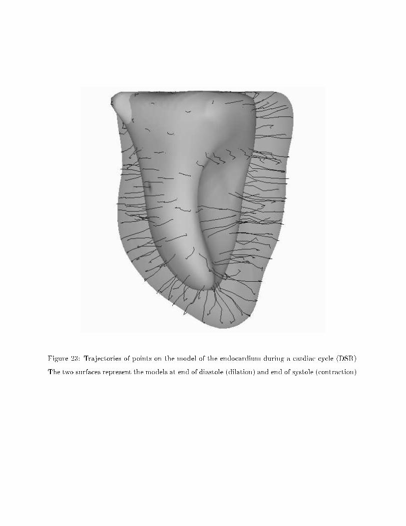
Analyzing heart deformation - submitted to MEDIA 34which cannot be easily detected. Figure 20 presents the trajectories found with the four strategiescompared to the original ones. One can see that the two temporal tracking methods (3 and 4)provide results which are close to the original trajectories, and catch the twist component of themotion, contrary to methods 1 and 2. Remark also that trajectories found with method 4 seemsmoother than the ones found with method 3. This is due to the use of only one FFD to recoverall the sequence.To quantify the twist component of the motion, once the trajectories have been computed, wedecompose the corresponding displacement vectors in cylindrical coordinates (see �gure 21):0BBBB@ xyz 1CCCCA! 0BBBBB@ � = px2 + y2� = arcos( xpx2 + y2 )z = z 1CCCCCA (9)The z-axis for the cylindrical representation correspond to the z-axis of inertia of the superellipsoidmodel. To measure the twist, we compute the di�erence of the � parameters for the two points thatrepresent the same parametric point during the contraction. Figure 22 represents the ranges ofthis twist, on the original synthetic data and for the models recovered by each of the four trackingmethods. Remark again that the twist component is pretty well recovered with the temporaltracking methods (3 and 4). The maximum value of � on the models is 27o for method 3 and 26ofor method 4 (to be compared with 30o).5.3.2 Experimental resultsFigures 23 and 24 show the trajectories of the node points between the end of diastole and the endof systole for the DSR and SPECT data. These are visualized from di�erent viewpoints to betterappreciate the motion. One can see, especially from the upper and lower viewpoints on �gure 24,that our tracking methods catch the characteristic twist component of the motion. Figure 25represents the mean values of �0� � (in radians) along the di�erent latitudes. One can see that thetwist is in the range 10 - 12 degrees which is the expected range.The pointwise tracking of the deformation allows an evaluation of the velocity �eld during thesequence. The visualization of these displacements by di�erent values, according to their range, onthe surface shows up clearly areas on the ventricle where the deformation is weak (see �gure 26).This visualization could be used by the physician to help localize pathologies like infarcted regions.


Figure 20: Trajectories on a synthetic example. Top: original trajectories. Bottom: trajectoriescomputed with strategies 1, 2, 3 and 4. Left column: view from the apex. Middle column: frontview. Right column: view from the base.

Analyzing heart deformation - submitted to MEDIA 36M

M’

,

x

y

z

ρ

, ρ

θθFigure 21: Cylindrical coordinates of two points M and M 0, which represent the same parametricpoint at the beginning and at the end of the cardiac cycle.6 ConclusionWe presented a new approach to analyze the deformation of the heart left ventricle with a parametricmodel. It is based on a parametric model that gives a compact representation of a set of points ina 3-D image. We presented four approaches using this model to track e�ciently the left ventriclewalls in a sequence of 3D images during a cardiac cycle and compared on synthetic and real data.The model is able to track simultaneously the endocardium and the epicardium walls, since it is avolumetric deformation. Experimental results have been shown for automatic shape tracking in atime sequence of cardiac images.The reconstruction and representation of a time sequence of surfaces by a sequence of parametricmodels has then allowed to infer some characteristic parameters useful to the physician, such asthe variation of the volume and heart wall thickness during a cardiac cycle, the ejection fractionand the twist component in the deformation of the ventricle.In some cases, the tracking can be helped by adding hard constraints when there is a prioriknowledge of the deformation at some reliable anchor points. This is the case in tagged images,where some tissues are marked and can be tracked after a simple preprocessing [2, 24, 44, 30, 27].We hope to apply our work to this recent technique of imaging in a the near future.

Analyzing heart deformation - submitted to MEDIA 37 ��

��

��

Figure 22: Twist component estimation on a synthetic example. Top: from original data. Fromleft to right and from top to bottom: from models obtained using strategies 1, 2, 3 and 4.


Figure 23: Trajectories of points on the model of the endocardium during a cardiac cycle (DSR).The two surfaces represent the models at end of diastole (dilation) and end of systole (contraction).


Figure 24: Trajectories of points on the model of the epicardium during a cardiac cycle from 2viewpoints (SPECT). The two surfaces represent the models at end of diastole (dilation) and endof systole (contraction).

Figure 25: Pro�le of the mean twist during the cardiac cycle along the z-axis (0 and 50 on the xaxis correspond to the positions of the two poles in the parameterization).

Analyzing heart deformation - submitted to MEDIA 40 ��

Figure 26: Range of the displacements of the points on the model during a cardiac cycle.AcknowledgementsWe would like to thank Grégoire Malandain who contributed to the segmentation of the imagespresented in this article; and Jérôme Declerck, Serge Benayoun and Alexis Gourdon for constructiveremarks; many thanks also to Lewis Gri�n for his careful review of this article. The images of theSPECT sequence were supplied by Prof. Michael Goris, from Stanford University. Thanks to Dr.Rich Robb and Dennis P. Hanson of Biomedical Imaging Resource, Mayo Foundation/Clinic forthe DSR data. This work was partially supported by Digital Equipment Corporation.A Calculation of the volume inside a meshFrom equations (6) and (7), considering an oriented mesh de�ned by a set of points and a set offacets, the volume inside the mesh can be written:V = 13 KXi=1 (OM;N) Si; (10)where K is the number of facets of the mesh.

Analyzing heart deformation - submitted to MEDIA 41We have to de�ne the normal vector of a facet. Assuming that the facet is de�ned by 3 pointsA1, A2 and A3, the normal vector can be written:Nd = (A1 �A2) ^ (A1 �A3) = A1 ^ A2 +A2 ^ A3 + A3 ^ A1;where (:^ :) denotes the vector product. Note that the norm of this normal vector is linked to thesurface S of the facet as follows: k Nd k= 2S . One can easily generalize this formula for a facetde�ned by a set of points Ai, i = 1::M :Nd = M�1Xi=1 (Ai ^ Ai+1) +AM ^ A1This expression can be seen as the average of the normal vectors of the decomposition of the facetinto triangular sub-facets.Let suppose that the mesh is composed of triangular facets de�ned by A1, A2 and A3. Thevolume Vi of the tetrahedron OA1A2A3 is: Vi = S:H3 ;where H is the height. Let O be the origin and G be the barycentre of a facet. Then:H = (OG;Nd)k Nd kAnd therefore: Vi = (OG;Nd)6This last expression is still true for a facet de�ned by M points. Finally, equation 10 can berewritten: V = 16 KXi=1 (OG;Nd)B Calcultion of the volume of a superellipsoidLet S be a superellipsoid surface de�ned by the following implicit equation:0B@� xa1� 2�2 + � ya2� 2�21CA�2�1 + � za3� 2�1 = 1: (11)

Analyzing heart deformation - submitted to MEDIA 42An explicit parameterization of S is given by:8>>>><>>>>: x = a1 cos�1 � cos�2 !y = a2 cos�1 � sin�2 !z = a3 sin�1 � ; ��2 � � � �2�� ! < �Due to the symmetry of the surface in relation to the 3 axes of the coordinate system, the compu-tation of the volume inside S can be made as follows:V = 2 Z a30 A(z) dz; (12)where A(z) is the area of a slice among the z-axis. For � = 0, the implicit equation of thecorresponding slice is: ( xa1 ) 2�2 + ( ya2 ) 2�2 = 1This leads to: A(0) = 4 a2 Z a10 y(x) dx = 4 a2 Z a10 [1� ( xa1 ) 2�2 ]�22 dxSetting: X = ( xa2 )�22 , it becomes:A(0) = 2 a1 a2 �2 �(�22 ; �22 + 1);where �(x; y) denotes the Beta function (Euler's integral of the �rst kind):�(x; y) = Z 10 tx�1(1� t)y�1 dtFinally, to calculate the volume inside S using equation 12, we have to write a1 and a2 as functionsof z. From the implicit de�nition of S (Equation 11), we deduce:a1(z) = a1[1� ( za3 ) 2�1 ]�12 ; a2(z) = a2[1� ( za3 ) 2�1 ]�12Therefore: V = 2 Z a30 2 �2 �(�22 ; �22 + 1) a1(z) a2(z) dzSetting: Z = ( za3 ) 2�1 , it becomes:V = 2 a1 a2 a3 �1 �2�(�22 ; �22 + 1) �(�12 ; �1 + 1)Note that for a sphere (�1 = �2 = 1; a1 = a2 = a3 = R), the previous formula gives:V = 2R3 B(12 ; 32)B(12 ; 2) = 43 � R3

Analyzing heart deformation - submitted to MEDIA 43Content of the videoThe video consists in 6 sequences:1. Nuclear medicine data (SPECT image). The �rst image of the sequence is visualized as aseries of 2D cross-sections (transverse slices). See section 3 for details.2. Segmentation of the SPECT sequence. See section 3 for details.3. Tracking of the epicardium (mesh) and the endocardium (rendered surface) in the SPECTsequence; on the left, the segmented surfaces, on the right, the reconstructed models. Seesections 3 and 4.2 for details.4. On the left, trajectories of the node points, on the right, velocity �eld during the SPECTsequence. See section 5.3.2 for details.5. Recovery of a twist motion on a synthetic example (1). Data with trajectories. See sec-tion 5.3.1 for details.6. Recovery of a twist motion on a synthetic example (2). Trajectories on the data and on themodels computed with tracking method 4. See section 5.3.1 for details.References[1] R. Acharya, R. Wasserman, J. Stevens, and C. Hinojosa. Biomedical imaging modalities: a tutorial.Computerized Medical Imaging and Graphics, 19(1):3�25, 1995.[2] A. Amini, R. Curwen, R. Constable, and J. Gore. MR physics-based snake tracking and dense deforma-tions from tagged cardiac images. In AAAI Symposium on Applications of Computer Vision to MedicalImage Processing, pages 126�129, Stanford, California, March 1994.[3] A. Amini and J. Duncan. Bending and stretching models for LV wall motion analysis from curves andsurfaces. Image and vision computing, 10:418�430, August 1992.[4] A. Amini, R. Owen, P. Anandan, and J. Duncan. Non-rigid motion models for tracking the left ven-tricular wall. In Information processing in medical images, Lecture notes in computer science, pages343�357, 1991. Springer-Verlag.[5] N. Ayache, J.D. Boissonnat, E. Brunet, L. Cohen, J.P. Chièze, B. Geiger, O. Monga, J.M. Rocchisani,and P. Sander. Building highly structured volume representations in 3D medical images. In ComputerAided Radiology, June 1989. Berlin, West-Germany.

Analyzing heart deformation - submitted to MEDIA 44[6] N. Ayache, J.D. Boissonnat, L. Cohen, B. Geiger, O. Monga, J. Levy-Vehel, and P. Sander. Stepstoward the automatic interpretation of 3D images. NATO ASI Series on 3D Imaging in Medicine, F60:107�120, 1990.[7] N. Ayache, P. Cinquin, I. Cohen, L. Cohen, F. Leitner, and O. Monga. Segmentation of complex 3Dmedical objects : a challenge and a requirement for computer assisted surgery planning and performing.MIT Press, 1994.[8] N. Ayache, I. Cohen, and I. Herlin. Medical Image Tracking, chapter 20. MIT Press, 1992.[9] R. Bajcsy and F. Solina. Three dimensional object representation revisited. In Proceedings IEEEInternational Conference on Computer Vision (ICCV), pages 231�240, London, June 1987.[10] E. Bardinet, L. Cohen, and N. Ayache. Fitting of iso-surfaces using superquadrics and free-form defor-mations. In Proceedings IEEE Workshop on Biomedical Image Analysis (WBIA), Seattle, Washington,June 1994.[11] E. Bardinet, L.D. Cohen, and N. Ayache. Superquadrics and free-form deformations: a global modelto �t and track 3D medical data. In Proceedings Conference on Computer Vision, Virtual Reality andRobotics in Medecine (CVRMed), Nice, France, April 1995.[12] S. Benayoun, N. Ayache, and I. Cohen. Adaptive meshes and nonrigid motion computation. In Pro-ceedings International Conference on Pattern Recognition (ICPR), Jerusalem, Israel, October 1994.[13] S. Benayoun, C. Nastar, and N. Ayache. Dense non-rigid motion estimation in sequences of 3D imagesusing di�erential constraints. In Proceedings Conference on Computer Vision, Virtual Reality andRobotics in Medecine (CVRMed), pages 309�318, Nice, France, April 1995.[14] A. Blake and A. Zisserman. Visual Reconstruction. MIT Press, 1987.[15] I. Cohen and L.D. Cohen. A hybrid hyperquadric model for 2-D and 3-D data �tting. In Proceed-ings International Conference on Pattern Recognition (ICPR), pages B�403�405, Jerusalem, October1994. Part of Inria TR 2188, to appear in Computer Vision, Graphics, and Image Processing : ImageUnderstanding.[16] I. Cohen, L.D. Cohen, and N. Ayache. Using deformable surfaces to segment 3-D images and in-fer di�erential structures. Computer Vision, Graphics, and Image Processing: Image Understanding,56(2):242�263, September 1992.[17] L.D. Cohen. On active contour models and balloons. Computer Vision, Graphics, and Image Processing:Image Understanding, 53(2):211�218, March 1991. INRIA TR 1075, August 1989.[18] L.D. Cohen. Auxiliary variables and two-step iterative algorithms in computer vision problems. Tech-nical report, Ceremade, Février 1995. Cahiers de Mathématiques de la Décision 9511, to appear inJournal of Mathematical Imaging and Vision and Proceedings ICCV'95, Boston.

Analyzing heart deformation - submitted to MEDIA 45[19] L.D. Cohen and I. Cohen. Finite element methods for active contour models and balloons for 2-D and3-D images. IEEE Transactions on Pattern Analysis and Machine Intelligence, 15(11), November 1993.[20] M. Davis, B. Rezaie, and F. Weiland. Assessment of left ventricular ejection fraction from technetium-99m-methoxy isobutyl isonitrile multiple-gated radionuclide angiocardoigraphy. IEEE Transactions onMedical Imaging, 12(2):189�199, June 1993.[21] J. Feldmar and N. Ayache. Locally a�ne registration of free-form surfaces. In Proceedings IEEEComputer Society Computer Vision and Pattern Recognition (CVPR), Seattle, USA, June 1994. Toappear in International Journal of Computer Vision.[22] M. Goris and J. Bretille. A colour atlas of nuclear cardiology. Chapman and Hall, 1992.[23] W. E. L. Grimson. From Images to Surfaces: A computational study of the Human Early vision system.The MIT Press, 1981.[24] M.A. Guttman, J.L. Prince, and E.R. McVeigh. Tag and Contour Detection in Tagged MR Images ofthe Left Ventricle. In IEEE Transactions on Medical Imaging, volume 13, pages 74�88, March 1994.[25] K. Höhne and W. Hanson. Interactive 3D segmentation of MRI and CT volumes using morphologicaloperations. Journal of Computer Assisted Tomography, 16(2):285�294, March 1992.[26] M. Kass, A. Witkin, and D. Terzopoulos. Snakes: active contour models. International Journal ofComputer Vision, 1:321�331, 1987.[27] S. Kumar and D. Goldgof. Automatic Tracking of SPAMM Grid and the Estimation of DeformationParameters from Cardiac MR Images. In IEEE Transactions on Medical Imaging, pages 122�132, March1994.[28] F. Leitner and P. Cinquin. Dynamic segmentation: Detecting complex topology 3D-object. In Proceed-ings International Conference of the IEEE Engineering in Medicine and Biology Society, pages 295�296,Orlando, Florida, November 1991.[29] T. McInerney and D. Terzopoulos. A dynamic �nite element surfacemodel for segmentation and trackingin multidimensionalmedical images with application to cardiac 4D image analysis. Computerized MedicalImaging and Graphics, 19:69�83, January 1995.[30] J. Park, D. Metaxas, and A. Young. Deformable models with parameter functions : application toheart-wall modeling. In Proceedings IEEE Computer Society Computer Vision and Pattern Recognition(CVPR), pages 437�442, June 1994.[31] A. Pentland and B. Horowitz. Recovery of nonrigid motion and structure. IEEE Transactions onPattern Analysis and Machine Intelligence, 13(7):730�742, July 1991.

Analyzing heart deformation - submitted to MEDIA 46[32] A.P. Pentland. Recognition by parts. In Proceedings IEEE International Conference on ComputerVision (ICCV), pages 612�620, 1987.[33] T.W. Sederberg and S.R. Parry. Free-form deformation of solid geometric models. Computer Graphics(Proceedings SIGGRAPH'86), 20(4):151�160, August 1986.[34] J. Serra. Image analysis and mathematical morphology, volume 1. Academic Press, 1982.[35] J. Serra. Image analysis and mathematical morphology: theoretical advances, volume 2. Academic Press,1988.[36] P. Shi, A. Amini, G. Robinson, A. Sinusas, C. Constable, and J. Duncan. Shape-based 4D left ventricularmyocardial function analysis. In Proceedings IEEE Workshop on Biomedical Image Analysis (WBIA),pages 88�97, Seattle, June 1994.[37] F. Solina and R. Bajcsy. Range image interpretation of mail pieces with superquadrics. In AAAI, pages733�737, Seattle, 1987.[38] F. Solina and R. Bajcsy. Recovery of parametric models from range images : The case for superquadricswith global deformations. IEEE Transactions on Pattern Analysis and Machine Intelligence, 12(2):131�147, February 1990.[39] R. Szeliski and S. Lavallée. Matching 3D anatomical surfaces with non-rigid deformations. In ProceedingsSPIE Geometric Methods in Computer Vision II, volume 2031, pages 306�315, San Diego, July 1993.Society of Photo-Optical Instrumentation Engineers.[40] R. Szeliski and S. Lavallée. Matching 3-d anatomical surfaces with non-rigid deformations using octree-splines. In Proceedings IEEE Workshop on Biomedical Image Analysis (WBIA), Seattle, Washington,June 1994.[41] D. Terzopoulos. The computation of visible-surface representations. IEEE Transactions on PatternAnalysis and Machine Intelligence, 10(4):417�438, July 1988.[42] D. Terzopoulos and D. Metaxas. Dynamic 3D models with local and global deformations: deformablesuperquadrics. IEEE Transactions on Pattern Analysis and Machine Intelligence, 13(7):703�714, July1991.[43] D. Terzopoulos, A. Witkin, and M. Kass. Symmetry-seeking models for 3D object reconstruction.International Journal of Computer Vision, 1(3):211�221, October 1987.[44] A.A. Young, D.L. Kraitchman, and L. Axel. DeformableModels for TaggedMR Images : Reconstructionof 2- and 3-Dimensional Heart Wall Motion. In IEEE Workshop on Biomedical Image Analysis, pages317�323, June 1994.

Analyzing heart deformation - submitted to MEDIA 47[45] A.L. Yuille, P.W. Hallinan, and D.S. Cohen. Feature extraction from faces using deformable templates.International Journal of Computer Vision, 8(2):99�111, September 1992.

analyzing deformation the left v en tricle of the heart ...cohen/mypapers/bardinetrr2797.… ·...

Documents