The following text is a preprint and extended version

(including mathematical derivations) of the paper:

N. Fries, M. Dreyer; An Analytic Solution of Capillary

Rise Restrained by Gravity; Journal of Colloid and

Interface Science 320: 259–263, 2008.

www.elsevier.com/locate/jcis or

http://dx.doi.org/10.1016/j.jcis.2008.01.009

This text is intended as online supplementary material.

An Analytic Solution of Capillary Rise Restrained by Gravity

N. Fries and M. Dreyer ∗Center of Applied Space Technology and Microgravity (ZARM), University of Bremen. Am Fallturm, 28359 Bremen, Germany

Abstract

We derive an analytic solution for the capillary rise of liquids in a cylindrical tube or a porous medium in terms of height h asa function of time t. The implicit t(h) solution by Washburn is the basis for these calculations and the Lambert W function isused for its mathematical rearrangement. The original equation is derived out of the 1D momentum conservation equation andfeatures viscous and gravity terms. Thus our h(t) solution, as it includes the gravity term (hydrostatic pressure), enables thecalculation of the liquid rise behavior for longer times than the classical Lucas-Washburn equation. Based on the new equationseveral parameters like the steady state time and the validity of the Lucas-Washburn equation are examined. The results are alsodiscussed in dimensionless form.

Key words: Capillary rise, Capillary tube, Analytic solution, Liquid penetration, Porous medium, Imbibition, Lucas-Washburn equation,

Washburn equation, Lambert W function

Introduction

Capillary driven flow is an important field of research asmany applications in science, industry and daily life relyon capillary transport. For example in hydrology the move-ment of groundwater is influenced by capillary transportas well as in heat pipes, spacecraft propellant managementdevices (PMDs), marker pens, candle wicks and sponges.Mostly this transport occurs in complex formed structures,however many flow or layout calculations adopt models forcylindric tubes to match the flow in arbitrary shaped cap-illaries. Often a porous medium, no matter how its poresare formed microscopically, can be described with sufficientprecision by the ”bundle of capillary tubes” model or theDarcy law. When regarding the behavior of a liquid broughtinto contact with a vertical, small tube (as shown in Fig. 1)it can be seen that at first a fairly fast flow into it will de-velop. Later the rising of the liquid will continuously slowdown until finally a steady state is reached. The descrip-tion of the liquid rise over time by mathematical methodsand its prediction are of great interest as can be seen fromthe following brief literature review. In 1918 Lucas [1] and1921 Washburn [2] are the first to give an analytic expla-nation of the rate of liquid rise in a capillary tube. Theyconsider a flow regime where the influence of inertia and

∗ Corresponding author.

E-mail address: dreyer@zarm.uni-bremen.de

Fig. 1. Setup for capillary driven flow showing the liquid reservoir

and a tube.

the influence of gravity can be neglected. In 1922 Rideal [3]and 1923 Bosanquet [4] try to expand the Lucas-Washburnsolution to cases including inertia and gravity by means ofseries expansion. 1976 Levine et al. [5] and [6] develop theo-ries for the capillary rise in tubes as well as in parallel platechannels. Marmur and Cohen [7], [8] characterize porousmedia by analyzing the kinetics of capillary penetration.Ichikawa and Satoda [9] describe the interface dynamics ofcapillary flow and derive dimensionless variables. In 1997Quere [10] investigates the capillary rise dominated by in-ertial forces and finds oscillations to occur if the fluid vis-cosity is low enough. Delker et al. [11] and Lago and Araujo[12] write about the rise of liquids in columns of glass beadsand find Lucas-Washburn behavior for small times, how-ever deviations for later times. In 2000 Zhmud et al. [13]

Preprint submitted to Elsevier 31 January 2008

give a good overview over the solutions for the differenttime regimes and derive short- and long time asymptoticsolutions. Siebold et al. [14] carry out capillary rise experi-ments in glass capillaries and packed powder to investigatethe effect of the dynamic contact angle. Hamraoui and Ny-lander [15] provide an analytical approach for setups witha highly dynamic contact angle. 2004 Chan et al. [16] givefactors affecting the significance of gravity on infiltrationof a liquid into a porous medium. Lockington and Parlange[17] find an equation for the capillary rise in porous media.Xue et al. [18] write about dynamic capillary rise with hy-drostatic effects. In a recent paper Chebbi [19] investigatesthe dynamics of liquid penetration and compares numeri-cal results with asymptotic solutions.To look at the problem in more detail the momentum bal-ance of a liquid inside a tube shall be presented. The fol-lowing assumptions hold: i) the flow is one dimensional, ii)no friction or inertia effects by displaced air occur, iii) noinertia or entry effects in the liquid reservoir, iv) the vis-cous pressure loss inside the tube is given by the Hagen-Poiseuille respectively the Darcy law both valid for laminarflow, and v) the constant capillary pressure can be calcu-lated with the static contact angle θ and the tube (or pore)radius R (see Appendix 1). With these assumptions themomentum balance of a liquid inside a capillary tube gives:

2σ cos θR

= ρgh sinψ +8µhR2

h+ ρd(hh)dt

. (1)

Here σ refers to the surface tension, R to the inner tuberadius, ρ to the fluid density, g to gravity and µ to thedynamic viscosity. In Eq. (1) the individual terms refer to(left to right):– The capillary pressure– The gravity term (hydrostatic pressure)– The viscous pressure loss (Hagen-Poiseuille)– The inertia term

Fig. 2. Setup with an inclined tube.

ψ (see Fig. 2) is the angle formed between the inclined tubeand the free liquid surface. It shall be mentioned that foran inclined setup the height h is not the absolute height inrelation to the liquid reservoir level but the distance coveredwithin the tube.

When it comes to the momentum equation of a liquid ina generic porous medium (see Fig. 3), the Darcy law canbe used. It gives the viscous pressure loss as

∇p = − µ

Kvs, (2)

where vs is the volume averaged velocity (superficial ve-locity) and K the permeability of the porous medium.Comparing the Hagen-Poiseuille law and Eq. (2) shows that

Fig. 3. Setup using a porous medium.

both laws are interchangeable with each other giving

R2 =8Kφ, (3)

with φ being the porosity of the material. The porosity isincluded as both laws are defined for the intersticial (Hagen-Poiseuille) and the superficial velocity (Darcy) respectively.Thus the momentum equation in a porous medium usingthe Darcy law reads

2σ cos θR

= ρgh sinψ +φµh

Kh+ ρ

d(hh)dt

. (4)

For porous media one possible approach to experimentallydetermine the two parameters R andK is to do a first eval-uation of the maximum reachable height (static case) toobtain the radius R for the capillary pressure. Later thepermeability K can be obtained by fitting the calculatedliquid rise curve to experimental values.The differential equations (1) and (4) cannot be easilysolved analytically, but numerical methods may be used.However, as an analytical solution is favorable, solutionscan be found for certain flow regimes where individualterms of Eqs. (1) and (4) can be neglected. Stange [20]claims that there are four time regimes. For small timesthe inertia term dominates, later the convective losses inthe entry region (not modeled here), then the viscous termand finally the hydrostatic term. For infinite times a steadystate is reached where the hydrostatic pressure balancesthe capillary pressure. As applications of capillary flow orexperiments are often bound to certain time regimes, it isfeasible to neglect the corresponding terms in Eq. (1) toobtain analytic solutions. In the following two of these willbe presented.

Viscous dominated flow

Lucas [1] 1918 and Washburn [2] 1921 consider a flowregime where the influence of inertia and the influence ofgravity can be neglected, thus simplifying Eq. (1) to

2

2σ cos θR

=8µhhR2

. (5)

Rearranging gives

hdh

dt=σR cos θ

4µ. (6)

Solving this ordinary differential equation with the initialcondition h(0) = 0 by means of separation of variables leadsto the well-established Lucas-Washburn equation:

h2 =σR cos θ

2µt. (7)

The Lucas-Washburn solution is probably the most usedequation when it comes to the characterization of capillarytransport or ”wicking” in capillary tubes, porous mediaor the capillarities in a pack of powder. Unfortunately thefairly simple - and thus nice to handle - Eq. (7) has somelimitations. For small times near zero the fluid velocity isapproaching infinity, which is not feasible. This discrep-ancy can be explained with the neglect of the inertia term.Also when flow is occurring in a vertical capillary undergravity there is no limit to the maximum reachable height,which originates from the neglect of the gravity term. In thefollowing sections the gravity term shall not be neglectedwhich still allows to give an analytic solution as alreadyshown by Washburn in 1921, however in terms of t(h) andnot h(t) as we seek it.

Viscous and hydrostatic dominated flow regime

To extend the just derived Lucas-Washburn equation toflows where gravity and thus hydrostatic pressure have tobe taken into account one is only allowed to neglect theinertia term of Eqs. (1) or (4) giving (here shown for Eq.(4)):

2σ cos θR

= ρgh sinψ +φµh

Kh. (8)

Rearranging gives

h =2σ cos θφµ

K

R

1h− ρKg sinψ

φµ, (9)

valid for h 6= 0 as there is a singularity.To simplify the equation one may introduce the constants

(capillary tube and Darcy version)

a =σR cos θ

4µ=

2σ cos θφµ

K

R(10)

and

b =ρgR2 sinψ

8µ=ρKg sinψ

φµ. (11)

Thus Eq. (9) reduces to

h =a

h− b. (12)

As mentioned above, an analytic solution to this differentialequation is given by Washburn [2] or Lukas and Soukupova[21]. It is calculated as follows: Eq. (12) can be rewritten as

dt =hdh

a− bh. (13)

After integration as shown in Appendix 2 one obtains

t = −hb− a

b2ln(a− bh) + C. (14)

To find the unknown constant C the initial condition

h(t→ 0) = 0 (15)

can be used to give

C =a

b2ln(a). (16)

This leads to following implicit analytic form

t = −hb− a

b2ln(

1− bh

a

), (17)

which is the result of Washburn or Lukas and Soukupovain terms of t = t(h). Hamraoui and Nylander [15] find thissolution to diverge as the liquid approaches the equilibriumheight. In 2000 Zhmud et al. [13] evolve a long term asymp-totic solution in terms of h(t), shown here rearranged as

h(t) =a

b(1− e− b2t

a ). (18)

To obtain a more accurate solution for h(t) we follow anew approach. Eq. (17) can be multiplied by −b2/a and bysubtracting 1 on both sides one obtains

−1− b2t

a=hb

a− 1 + ln

(1− bh

a

), (19)

which by taking the power of e gives after rearrangement

−e−1− b2ta =

(hb

a− 1)e

hba −1. (20)

At this point the Lambert W function W (x) named afterJohann Heinrich Lambert, and defined by an inverse expo-nential function

x = W (x)eW (x) (21)can be used to solve for h. It can be seen that Eq. (20)follows the form

y(t) = x(h)ex(h). (22)

By definition the W function can be written as

y(t) = W (y(t))eW (y(t)). (23)

Relating Eq. (22) and Eq. (23) gives

x(h)ex(h) = W (y(t))eW (y(t)). (24)

From this it can be seen that

x(h) = W (y(t)). (25)

Coming back to Eq. (20) the inverse properties of the Lam-bert W function can be used to give

bh

a− 1 = W

(−e−1− b2t

a

). (26)

After rearranging one obtains

h(t) =a

b

[1 +W (−e−1− b2t

a )], (27)

which is a full analytic solution in terms of h = h(t), andcan be verified as shown in Appendix 3. From now on we will

3

refer to it as the extended solution. In Fig. 4 this extendedsolution is calculated and plotted for a setup using siliconfluid (0.93 cSt) in a 0.1 mm radius borosilicate glass cap-illary. The material properties are found to be θs = 16.3◦,µ = 7.6× 10−4 Pa s and σ = 15.9× 10−3 N/m. The otherlines in Fig. 4 refer to the Lucas-Washburn equation (Eq.(7)) and the long time asymptotic solution by Zhmud etal. [13] (Eq. (18)). The two numerical simulations are cal-culated with constant contact angle and dynamic contactangle as done by Chebbi [19], respectively. For the numericsimulations inertia is neglected and for the dynamic contactangle the equation given by Jiang et al. [22] (see Appendix1) is used.

Fig. 4. Diagram showing the different solutions for silicon fluid 0.93

cSt in a 0.1 mm radius borosilicate glass capillary. Height h is plottedversus time t.

For certain cases it might be of interest to consider a moregeneral definition of the initial condition (Eq. (15)) like

h(t0) = h0. (28)

This leads to

h(t) =a

b

[1 +W

((−a+ bh0)e−1+

b(bt0+h0−bt)a

a

)], (29)

as is shown in Appendix 4. Regarding Eq. (29) it can beseen that for t0 = 0 and h0 = 0 it is equal to Eq. (27), theextended solution derived before.

Further information on the Lambert W function as de-fined in Eq. (21), and its applications shall be given [23],[24] and [25]. Its solutions are partly in the complex plane,but switch to real values for −1/e ≤ x as shown in Fig. 5.Also, the Lambert W function has been used to solve dif-ferential equations before. For example in 1993 Barry et al.[26] use the Lambert W function to give an analytical so-lution to a transcendental equation related to the problemthe present work deals with. To calculate water movementin unsaturated soil they use a differential equation whichis a simplified form of Eq. (12) with a = b (here shown re-arranged and in our variables)

h =a

h− a. (30)

Solving for the initial condition h(t → 0) = 0 gives anequation featuring the Lambert W function

Fig. 5. Upper branch of the Lambert W function for −1/e ≤ x ≤ 5.

h(t) = 1 +W (−e−1−at). (31)

Barry et al. mention that it can be used to calculate infil-tration as well as capillary rise of moisture in soils.

Practical evaluation of the Lambert W function

When applying Eq. (27) to practical problems it is impor-tant to be able to calculate the numeric value of the Lam-bert W function. In many commercial mathematical pro-grams the Lambert W function is already included with itscall being W[x] or ProductLog[x]. It is also possible to usespreadsheet calculation programs that don’t feature Lam-bert W. In this case it is required to use an approximationexpression forW (x) that covers the relevant range. For ourcase such an approximate function is given by Barry et al.[26] (slightly rearranged) as

W (x) ≈ −1 +√

2 + 2ex

1 + 4.13501√

2+2ex12.7036+

√2+2ex

, (32)

with e being Euler’s number. This equation accounts forthe relevant range of −e−1 ≤ x ≤ 0 (upper branch) with amaximum relative error of 0.1%.

Steady state time

Regarding Eq. (27) one may notice that for infinite timethe height gain converges into a maximum value hmax. Thisis the point where the hydrostatic pressure balances thecapillary pressure, or mathematicallyW (0) = 0. This gives

hmax = h(t→∞) =a

b=

2σ cos θRρg sinψ

. (33)

Here a and b are defined by Eqs. (10) and (11). As h ap-proaches hmax at some point the height increase is so smallthat one may speak of a steady state. To find the timeneeded to reach this point, we define the steady state timets to be exactly that time where h has reached 99% of hmax.Thus one may write

h(ts) = 0.99hmax. (34)

Using Eq. (33) and Eq. (27) gives

4

0.99a

b=a

b(1 +W (−e−1− b2ts

a )). (35)

After rearranging one obtains

−0.01 = W (−e−1− b2tsa ), (36)

and with Eq. (21)

−0.01e−0.01 = −e−1− b2tsa . (37)

To obtain ts

−1− b2tsa

= ln(0.01)− 0.01, (38)

and finally

ts =a

b2(− ln(0.01) + 0.01− 1) ≈ 3.62a

b2. (39)

This may also be written with all variables to give

ts = 3.6216σµ cos θ

R3ρ2g2 sin2 ψ= 3.62

2φσµ cos θRρ2g2K sin2 ψ

. (40)

Flow velocity

To obtain the flow velocity h(t) it is necessary to differ-entiate the height h(t). For the Lucas-Washburn equationone obtains

h(t) =√a

2t, (41)

while using the extended solution including gravity yields

h(t) =−b W (−e−1− b2t

a )

1 +W (−e−1− b2ta )

. (42)

Both velocity functions are only defined for t > 0. Furtherdetails on differentiating the Lambert W function can befound in Appendix 3.

Dimensional analysis

To generalize the obtained solutions the introduction ofdimensionless numbers is always of interest. Zhmud et al.[13] use

h∗ =h(t)hmax

, (43)

and

t∗ =ρgr2t

8µhmax. (44)

Ichikawa and Satoda [9] give dimensionless numbers thatalso allow to account for the dynamic contact angle. Forthe time they find

t∗ =t

T0, (45)

where T0 is defined as the characteristic time of viscouseffects

T0 =ρD2

32µ. (46)

To scale the height they use following expression

h∗ =

√128Me

h

D, (47)

where Me is defined as Reynolds number divided by Cap-illary number

Me =σ0ρD

µ2. (48)

Here σ0 refers to the static surface tension. Ichikawa andSatoda scale the driving force by

Df =σ cos θσ0

+Bo4, (49)

where Bo is the Bond number as given in Eq. (52). In ourwork, regarding Eqs. (39) and (40) we derive a dimension-less number for the time, the ”capillary time number” TN

TN = tb2

a=

tρ2g2R3 sin2 ψ

16σµ cos θ=

tRρ2g2Ksin2 ψ

2φσµ cos θ. (50)

This TN can be transferred to t∗ (Eq. (44)) used by Zhmudet al.. The TN can be interpreted as a specialized form ofthe following term:

(Gravity force)2

Viscous force× Surface tension force=

Bo2

Ca, (51)

with the Bond number relating gravity forces to surfacetension forces

Bo =ρg sinψR2

σ, (52)

and the Capillary number relating viscous forces to surfacetension forces being

Ca =µvσ∼ µR

σt. (53)

From Eq. (39) it can be derived that if TN is larger than3.62 a steady state has been reached as shown in Fig. 6.To give a dimensionless number including the height, the”capillary height number” HN, one may relate the height hto the maximum obtainable height hmax as done by Zhmudet al.

HN = hba

=hRρg sinψ2σ cos θ

. (54)

The HN can also be regarded as a ”capillary Bond number”since it relates gravity forces to surface tension forces.Using these dimensionless numbers the Lucas-Washburnequation (Eq. (7)) as well as the extended solution (Eq.(27)) can be made dimensionless giving

HN =√

2TN, (55)

for the Lucas-Washburn equation and

HN = 1 + W(−e−1−TN) (56)

for the extended solution including the gravity term. Fig. 6shows that in the beginning the Lucas-Washburn solutionfits very good to the extended solution (Eq. (27)), howevertends to deviate to higher values for longer times due tothe neglect of gravity. For TN > 3.62 the extended solutionreaches a steady state. Regarding the velocity of the ex-

5

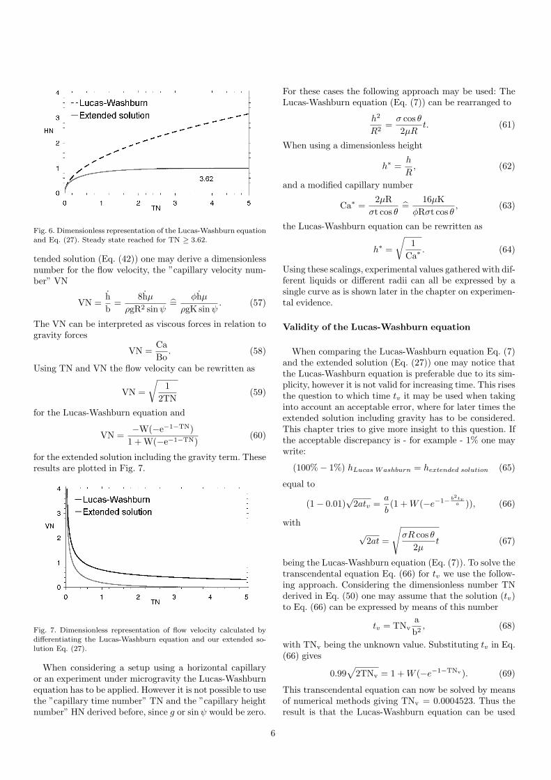
Fig. 6. Dimensionless representation of the Lucas-Washburn equation

and Eq. (27). Steady state reached for TN ≥ 3.62.

tended solution (Eq. (42)) one may derive a dimensionlessnumber for the flow velocity, the ”capillary velocity num-ber” VN

VN =hb

=8hµ

ρgR2 sinψ=

φhµρgK sinψ

. (57)

The VN can be interpreted as viscous forces in relation togravity forces

VN =CaBo

. (58)

Using TN and VN the flow velocity can be rewritten as

VN =

√1

2TN(59)

for the Lucas-Washburn equation and

VN =−W(−e−1−TN)

1 + W(−e−1−TN)(60)

for the extended solution including the gravity term. Theseresults are plotted in Fig. 7.

Fig. 7. Dimensionless representation of flow velocity calculated by

differentiating the Lucas-Washburn equation and our extended so-lution Eq. (27).

When considering a setup using a horizontal capillaryor an experiment under microgravity the Lucas-Washburnequation has to be applied. However it is not possible to usethe ”capillary time number” TN and the ”capillary heightnumber” HN derived before, since g or sinψ would be zero.

For these cases the following approach may be used: TheLucas-Washburn equation (Eq. (7)) can be rearranged to

h2

R2=σ cos θ2µR

t. (61)

When using a dimensionless height

h∗ =h

R, (62)

and a modified capillary number

Ca∗ =2µR

σt cos θ=

16µKφRσt cos θ

, (63)

the Lucas-Washburn equation can be rewritten as

h∗ =

√1

Ca∗. (64)

Using these scalings, experimental values gathered with dif-ferent liquids or different radii can all be expressed by asingle curve as is shown later in the chapter on experimen-tal evidence.

Validity of the Lucas-Washburn equation

When comparing the Lucas-Washburn equation Eq. (7)and the extended solution (Eq. (27)) one may notice thatthe Lucas-Washburn equation is preferable due to its sim-plicity, however it is not valid for increasing time. This risesthe question to which time tv it may be used when takinginto account an acceptable error, where for later times theextended solution including gravity has to be considered.This chapter tries to give more insight to this question. Ifthe acceptable discrepancy is - for example - 1% one maywrite:

(100%− 1%) hLucas Washburn = hextended solution (65)

equal to

(1− 0.01)√

2atv =a

b(1 +W (−e−1− b2tv

a )), (66)

with√

2at =

√σR cos θ

2µt (67)

being the Lucas-Washburn equation (Eq. (7)). To solve thetranscendental equation Eq. (66) for tv we use the follow-ing approach. Considering the dimensionless number TNderived in Eq. (50) one may assume that the solution (tv)to Eq. (66) can be expressed by means of this number

tv = TNvab2, (68)

with TNv being the unknown value. Substituting tv in Eq.(66) gives

0.99√

2TNv = 1 +W (−e−1−TNv). (69)

This transcendental equation can now be solved by meansof numerical methods giving TNv = 0.0004523. Thus theresult is that the Lucas-Washburn equation can be used

6

up to t = 0.0004523a/b2 when accepting an error of 1%.The height reached at this point may again be expressed interms of HN

HNv =hv

hmax= 1 + W(−e−1−TNv), (70)

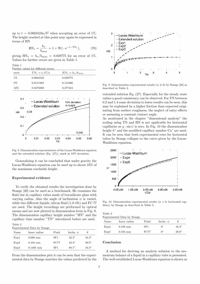
giving HNv = hv/hmax = 0.029775 for an error of 1%.Values for further errors are given in Table 1.

Table 1Further values for different errors

error TNv = tv b2/a HNv = hv/hmax

1% 0.0004523 0.029775

5% 0.0115465 0.144366

10% 0.0475088 0.277424

Fig. 8. Dimensionless representation of the Lucas-Washburn equationand the extended solution (Eq. (27)), mark at 10% deviation.

Generalizing it can be concluded that under gravity theLucas-Washburn equation can be used up to about 10% ofthe maximum reachable height.

Experimental evidence

To verify the obtained results the investigation done byStange [20] can be used as a benchmark. He examines thefluid rise in capillary tubes made of borosilicate glass withvarying radius. Also the angle of inclination ψ is varied,while two different liquids, silicon fluid (1.0 cSt) and FC 77are used. The height recordings are performed by opticalmeans and are now plotted in dimensionless form in Fig. 9.The dimensionless capillary height number ”HN” and thecapillary time number ”TN” introduced before are used.

Table 2

Experimental Data by Stange

Name Inner radius Fluid Inclin. ψ θ

Exp1 0.088 mm SF1 32.3◦ 16.3◦

Exp2 0.104 mm FC77 32.3◦ 28.0◦

Exp3 0.1405 mm SF1 88.7◦ 16.3◦

From the dimensionless plot it can be seen that the experi-mental data by Stange matches the values predicted by the

Fig. 9. Dimensionless experimental results (ψ 6= 0) by Stange [20] as

described in Table 2.

extended solution Eq. (27). Especially for the steady statevalues a good consistency can be observed. For TN between0.2 and 1.4 some deviation to lower results can be seen, thismay be explained by a higher friction than expected origi-nating from surface roughness, the neglect of entry effectsor assuming a constant contact angle.As mentioned in the chapter ”dimensional analysis” thescaling using TN and HN is not applicable for horizontalcapillaries as g · sinψ is zero. In Fig. 10 the dimensionlessheight h∗ and the modified capillary number Ca∗ are used.It can be seen that both experimental rows for horizontaltubes by Stange collapse to the curve given by the Lucas-Washburn equation.

Fig. 10. Dimensionless experimental results (ψ = 0, horizontal cap-illary) by Stange as described in Table 3.

Table 3Experimental Data by Stange

Name Inner radius Fluid Inclin. ψ θ

Exp4 0.109 mm SF1 0◦ 16.3◦

Exp5 0.104 mm FC77 0◦ 28.0◦

Conclusion

A method for deriving an analytic solution to the mo-mentum balance of a liquid in a capillary tube is presented.The well-established Lucas-Washburn equation is shown as

7

well as an extended solution introduced. The extended so-lution includes the gravity term (hydrostatic pressure) andenables the calculation of the liquid rise behavior for longertimes. The time necessary to reach a steady state is exam-ined and several relevant dimensionless numbers are found.By means of these numbers a dimensionless plot of theLucas-Washburn equation and the extended solution in-cluding gravity can be plotted. The flow velocity is obtainedby differentiating the height and a dimensionless numberfor its description is found. Also the error made when ne-glecting gravity and using the Lucas-Washburn equation isdetermined. As an outlook it can be stated that derivingfurther analytical solutions to the momentum equation isstill of great interest, as it could lead to a solution that isalso valid for shortest time regimes at the beginning of thecapillary rise process.

Acknowledgement

The funding of the research project by the German Fed-eral Ministry of Education and Research (BMBF) throughthe Research Training Group PoreNet is gratefully ac-knowledged.

References

[1] R. Lucas. Ueber das Zeitgesetz des kapillaren Aufstiegs von

Flussigkeiten. Kolloid-Zeitschrift, 23:15–22, 1918.[2] E.W. Washburn. The dynamics of capillary flow. Physical

Review, 17(3):273–283, 1921.[3] E.K. Rideal. On the flow of liquids under capillary pressure.

Philos. Mag. Ser. 6, 44:1152–1159, 1922.[4] C.H. Bosanquet. On the flow of liquids into capillary tubes.

Philos. Mag. Ser. 6, 45:525–531, 1923.[5] S. Levine, P. Reed, E.J. Watson, G. Neale. A theory of the rate

of rise of a liquid in a capillary. In M. Kerker, editor, Colloid and

Interface Science, volume 3, pages 403–419. Academic Press,

New York, 1976.[6] S. Levine, J. Lowndes, E.J. Watson, G. Neale. A theory of

capillary rise of a liquid in a vertical cylindrical tube and in a

parallel-plate channel. J. Colloid Interface Sci., 73(1):136–151,1980.

[7] A. Marmur. Penetration and displacement in capillary systems

of limited size. Adv. Colloid Interface Sci., 39:13–33, 1992.[8] A. Marmur, R.D. Cohen. Characterization of porous media by

the kinetics of liquid penetration: The vertical capillaries model.

J. Colloid Interface Sci., 189(2):299–304, 1997.[9] N. Ichikawa, Y. Satoda. Interface dynamics of capillary flow in

a tube under negligible gravity condition. J. Colloid Interf. Sci.,

162:350–355, 1994.[10] D. Quere. Inertial capillarity. Europhys. Lett., 39(5):533–538,

1997.[11] T. Delker, D.B. Pengra, P.-Z. Wong. Interface pinning and the

dynamics of capillary rise in porous media. Physical ReviewLetters, 76(16):2902–2905, 1996.

[12] M. Lago, M. Araujo. Capillary rise in porous media. Physica

A, 289:1–17, 2001.[13] B.V. Zhmud, F. Tiberg, K. Hallstensson. Dynamics of capillary

rise. J. Colloid Interface Sci., 228(2):263–269, 2000.[14] A. Siebold, M. Nardin, J. Schultz, A. Walliser, M. Oppliger.

Effect of dynamic contact angle on capillary rise phenomena.

Colloids and Surfaces A, 161(1):81–87, 2000.

[15] A. Hamraoui, T. Nylander. Analytical approach for the Lucas-Washburn equation. J. Colloid Interf. Sci., 250:415–421, 2002.

[16] T.-Y. Chan, C.-S. Hsu, S.-T. Lin. Factors affecting thesignificance of gravity on the infiltration of a liquid into a porous

solid. J. Porous Mat., 11(4):273–277, 2004.

[17] D.A. Lockington, J.-Y. Parlange. A new equation formacroscopic description of capillary rise in porous media. J.

Colloid Interf. Sci., 278:404–409, 2004.

[18] H.T. Xue, Z.N. Fang, Y. Yang, J.P. Huang, L.W. Zhou. Contact

angle determined by spontaneous dynamic capillary rises with

hydrostatic effects: Experiment and theory. Chemical PhysicsLetters, 432:326–330, 2006.

[19] R. Chebbi. Dynamics of liquid penetration into capillary tubes.

J. Colloid Interface Sci., 315:255–260, 2007.

[20] M. Stange. Dynamik von Kapillarstromungen in zylindrischen

Rohren. Cuvillier, Gottingen, 2004.

[21] D. Lukas, V. Soukupova. Recent studies of fibrous materials

wetting dynamics. In INDEX 99 Congress, Geneva, Switzerland,

1999.

[22] T.-S. Jiang, S.-G. Oh, J.C. Slattery. Correlation for dynamic

contact angle. J. Colloid Interf. Sci., 69:74–77, 1979.

[23] B. Hayes. Why W. American Scientist, the magazine of Sigma

Xi, The Scientific Research Society, 93:104–109, 2005.

[24] R.M. Corless, G.H. Gonnet, D.E.G. Hare, D.J. Jeffrey, D.E.

Knuth. On the Lambert W Function. Advances in

Computational Mathematics, 5:329–359, 1996.

[25] S.R. Valluri, D.J. Jeffrey, R.M. Corless. Some Applications of

the Lambert W Functions to Physics. Canadian Journal of

Physics, 78:823–831, 2000.

[26] D.A. Barry, J.-Y. Parlange, G.C. Sander, M. Sivaplan. A class

of exact solutions for Richards’ equation. Journal of Hydrology,142:29–46, 1993.

[27] R.L. Hoffman. A study of the advancing interface. I. Interfaceshape in liquid-gas systems. J. Colloid Interface Sci., 50:228–

241, 1975.

[28] M. Bracke, F. De Voeght, P. Joos. The kinetics of wetting: thedynamic contact angle. Progress in Colloid & Polymer Science,

79:142–149, 1989.

Appendix 1

When a liquid-gas interface is subject to motion the dy-namic contact angle θd formed between the liquid and solidis different from the static contact angle θs. Jiang et al. [22](based on data by Hoffman [27]) give the following corre-lation for the dynamic contact angle

cos θd − cos θs

cos θs + 1= − tanh(4.94Ca0.702), (71)

where the capillary number is defined as

Ca =µhσ. (72)

Bracke et al. [28] find

cos θd − cos θs

cos θs + 1= −2Ca0.5. (73)

When considering silicon fluid (0.93 cSt) in a borosilicateglass capillary (like in Fig. 4) and using some arbitrary riserates one obtains the values shown in Table 4. Coming backto the numerical simulation presented in Fig. 4 (capillaryradius is 0.1 mm) Figs. 11 and 12 show further results ofthe simulation featuring the dynamic contact angle. Due to

8

Table 4Calculated values of the dynamic contact angle for different capillary

rise rates. ”eff. dev.” refers to the effective deviation of the cosine

values of the dynamic vs. static contact angle.

Jiang et al. Bracke et al.

h [mm/s] θd [◦] eff. dev. [%] θd [◦] eff. dev. [%]

1 18.04 0.94 21.14 2.83

5 21.26 2.90 25.94 6.31

10 23.87 4.72 29.06 8.93

50 34.95 14.6 39.81 20.0

Fig. 11. Numerical results (interface velocity) for silicon fluid (0.93

cSt) in a 0.1 mm capillary.

Fig. 12. Dynamic contact angle for same simulation.

the small deviation between the simulation with the staticcontact angle and the dynamic one it can be concluded thatassuming a constant contact angle is feasible for capillaryrise in the investigated flow regime as typical contact linerise rates (depending on radius, viscosity etc.) are mostlyfound to be in the range of some mm/s. However one mustbe aware that for very large capillaries and short times thecontact angle can not be assumed as constant and inertiaeffects may as well be significant.

Appendix 2

To solve the integral of Eq. (13) the following approachmay be used:

t =∫

h

a− bhdh =

∫(bh− a) + a

b(a− bh)dh. (74)

This may be rearranged to

t =∫−1bdh+

∫a

b

1a− bh

dh. (75)

Preparing the substitution

y = a− bh (76)

bydy = −bdh (77)

gives

t =∫−1bdh−

∫a

b21ydy. (78)

Solving and reversing the substitute gives

t = −hb− a

b2ln(y) = −h

b− a

b2ln(a− bh). (79)

Appendix 3

To show that the extended solution Eq. (27) fulfills thedifferential equation (Eq. (12)) one may use the derivativeof the solution and put it back into the initial differentialequation.

By differentiating the defining Eq. (21) forW (x) [24] oneobtains

dx

dW (x)= eW (x) +W (x)eW (x). (80)

Rearranging gives

W ′(x) =1

eW (x) +W (x)eW (x), (81)

furtherW ′(x) =

1eW (x)(1 +W (x))

, (82)

and

W ′(x) =W (x)

W (x)eW (x)(1 +W (x)). (83)

Per definitionem:

x = W (x)eW (x) (84)

and finally

W ′(x) =W (x)

x(1 +W (x)). (85)

To ease the handling of Eq. (27) a coefficient z can be de-fined:

z = −e−1− b2ta , (86)

the derivative isdz

dt= z

−b2

a. (87)

Putting Eq. (85), Eq. (87) (the inner derivative) and Eq.(27) into Eq. (12) gives

a

b

W (z)z(1 +W (z))

z−b2

a=

ab

a(1 +W (z))− b. (88)

After some rearrangement one obtains

−b2

bW (z) =

−b2

bW (z) (89)

which proves that Eq. (27) is a solution to Eq. (12).

9

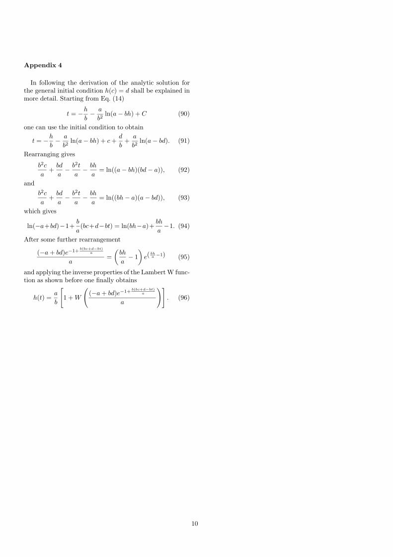
Appendix 4

In following the derivation of the analytic solution forthe general initial condition h(c) = d shall be explained inmore detail. Starting from Eq. (14)

t = −hb− a

b2ln(a− bh) + C (90)

one can use the initial condition to obtain

t = −hb− a

b2ln(a− bh) + c+

d

b+a

b2ln(a− bd). (91)

Rearranging gives

b2c

a+bd

a− b2t

a− bh

a= ln((a− bh)(bd− a)), (92)

andb2c

a+bd

a− b2t

a− bh

a= ln((bh− a)(a− bd)), (93)

which gives

ln(−a+bd)−1+b

a(bc+d−bt) = ln(bh−a)+ bh

a−1. (94)

After some further rearrangement

(−a+ bd)e−1+b(bc+d−bt)

a

a=(bh

a− 1)e(

bha −1) (95)

and applying the inverse properties of the Lambert W func-tion as shown before one finally obtains

h(t) =a

b

[1 +W

((−a+ bd)e−1+

b(bc+d−bt)a

a

)]. (96)

10