analytical evaluation of inorganic polymer …
TRANSCRIPT
ANALYTICAL EVALUATION OF INORGANIC POLYMER MATERIALS FOR
INFRASTRUCTURE REPAIR
By
ADITYA MANTHA
A thesis submitted to the
Graduate School-New Brunswick
Rutgers, The State University of New Jersey
in partial fulfillment of the requirements
for the degree of
Master of Science
Graduate Program in Civil and Environmental Engineering
written under the direction of
Dr. Husam Najm
and approved by
________________________
________________________
________________________
New Brunswick, New Jersey
October, 2014
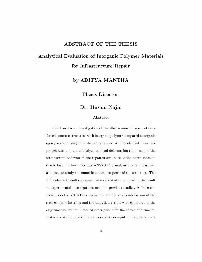
ABSTRACT OF THE THESIS
Analytical Evaluation of Inorganic Polymer Materials
for Infrastructure Repair
by ADITYA MANTHA
Thesis Director:
Dr. Husam Najm
Abstract
This thesis is an investigation of the effectiveness of repair of rein-
forced concrete structures with inorganic polymer compared to organic
epoxy system using finite element analysis. A finite element based ap-
proach was adopted to analyze the load deformation response and the
stress strain behavior of the repaired structure at the notch location
due to loading. For this study ANSYS 14.5 analysis program was used
as a tool to study the numerical based response of the structure. The
finite element results obtained were validated by comparing the result
to experimental investigations made in previous studies. A finite ele-
ment model was developed to include the bond slip interaction at the
steel concrete interface and the analytical results were compared to the
experimental values. Detailed descriptions for the choice of elements,
material data input and the solution controls input in the program are
ii
provided in this study. The results from this study showed that the
load deflection response of beam repaired with inorganic polymer is
similar to the control specimens. The study also showed the effect of
bond slip at the interface between steel and concrete on the load de-
flection response. The conclusions and recommendations of this study
are mentioned for further investigation related to this study.
iii

Acknowledgments
This research was performed under the supervision of Dr. Husam Najm. I
am extremely grateful to Dr Najm for his patience, knowledge and support
in helping me complete this thesis. I am grateful to Dr. P.N Balaguru for
having his door open for me to listen to my questions and give advice. Special
thanks to Dr. YK Yong for his valuable inputs and guidance.
My deepest gratitude is to my family. I have been amazingly fortunate to
have such a wonderful family. Without the encouragement and motivation
from my family this accomplishment would not have been possible. I would
like to thank my many dear friends for listening to me, offering me advice
and supporting me through the entire process.
.
iv
Contents
Abstract ii
Acknowledgments iv
1 Introduction 1
1.1 Epoxy Systems . . . . . . . . . . . . . . . . . . . . . . . . . . 4
1.2 Inorganic Systems . . . . . . . . . . . . . . . . . . . . . . . . . 10
1.3 Finite Element Based Approach . . . . . . . . . . . . . . . . . 14
2 Model description and Analytical investigation 16
2.1 General . . . . . . . . . . . . . . . . . . . . . . . . . . . . . . 16
2.2 FE Modeling Of Steel Reinforcement . . . . . . . . . . . . . . 17
2.3 Element selection . . . . . . . . . . . . . . . . . . . . . . . . . 20
2.3.1 SOLID 65 . . . . . . . . . . . . . . . . . . . . . . . . . 20
2.3.2 Link180 . . . . . . . . . . . . . . . . . . . . . . . . . . 21
2.3.3 Solid45 . . . . . . . . . . . . . . . . . . . . . . . . . . . 21
2.4 Real Constants . . . . . . . . . . . . . . . . . . . . . . . . . . 22
2.5 Material Properties . . . . . . . . . . . . . . . . . . . . . . . . 24
2.5.1 Concrete . . . . . . . . . . . . . . . . . . . . . . . . . . 24
2.5.2 Steel Reinforcement and Steel Plates . . . . . . . . . . 29
2.5.3 Epoxy . . . . . . . . . . . . . . . . . . . . . . . . . . . 31
2.5.4 Inorganic Polymer . . . . . . . . . . . . . . . . . . . . 32
2.6 Model Description . . . . . . . . . . . . . . . . . . . . . . . . 33
v
2.6.1 Beam Models I and II . . . . . . . . . . . . . . . . . . 34
2.6.2 Slab Model . . . . . . . . . . . . . . . . . . . . . . . . 42
3 Analysis Results And Discussion 48
3.1 Analysis . . . . . . . . . . . . . . . . . . . . . . . . . . . . . . 49
3.2 Results And Discussion . . . . . . . . . . . . . . . . . . . . . . 53
3.2.1 Effect Of Bond Slip On Load vs Deformation Response
Of Beams . . . . . . . . . . . . . . . . . . . . . . . . . 54
3.2.2 Beam Model I . . . . . . . . . . . . . . . . . . . . . . . 59
3.2.3 Beam Model II . . . . . . . . . . . . . . . . . . . . . . 67
3.2.4 Slab Model . . . . . . . . . . . . . . . . . . . . . . . . 72
4 Conclusions and Recommendations 75
A Appendix 81
A.1 Comparison Between Full Volume Model and Quarter Volume
Model . . . . . . . . . . . . . . . . . . . . . . . . . . . . . . . 81
A.2 Effect of Elastic Modulus of Filler Material on Stiffness . . . . 83
A.3 Effect of Shear Retention . . . . . . . . . . . . . . . . . . . . . 87
vi
List of Figures
1.1 Delaminated Concrete(Concreteanswers.org) . . . . . . . . . . 3
1.2 Kansas DOT’s Custom Chuck(Klein) . . . . . . . . . . . . . . 7
1.3 Insertable Gasket Type Injection Probe(Klein) . . . . . . . . . 8
1.4 Surface Mounted Type Injection Probe(Klein) . . . . . . . . . 8
1.5 Chemical Structure Of Potassium Polysialate(Davidovits) . . . 11
2.1 Newton-Raphson Iterative Solution . . . . . . . . . . . . . . . 17
2.2 Models For Reinforcement In Reinforced Concrete;(a) Dis-
crete;(b) Embedded;(c) Smeared(Tavarez,2001) . . . . . . . . 18
2.3 Solid65-3D Reinforced Concrete Solid element in ANSYS . . . 20
2.4 Link180-3D Spar element in ANSYS . . . . . . . . . . . . . . 21
2.5 Solid45-3D Solid element in ANSYS . . . . . . . . . . . . . . . 22
2.6 Typical uniaxial compressive and tensile stress-strain curve for
concrete (Bangash 1989) . . . . . . . . . . . . . . . . . . . . . 24
2.7 Simplified stress-strain model of concrete in compression . . . 27
2.8 3-D failure surface for concrete in ANSYS (Kachlakev 2000) . 28
2.9 Stress-strain curve for steel reinforcement . . . . . . . . . . . . 30
2.10 Stress-strain curve for Sealboss epoxy . . . . . . . . . . . . . . 31
2.11 Stress-strain curve for Inorganic Polymer . . . . . . . . . . . . 32
2.12 Input Parameters for Inorganic Polymer . . . . . . . . . . . . 33
2.13 ANSYS Model Of Quarter Beam . . . . . . . . . . . . . . . . 35
vii
2.14 FE Mesh of the Concrete,Steel Plate,and Steel Support Beam
for Model I . . . . . . . . . . . . . . . . . . . . . . . . . . . . 35
2.15 FE Mesh of the Concrete,Steel Plate,and Steel Support Beam
for Model II . . . . . . . . . . . . . . . . . . . . . . . . . . . . 36
2.16 Steel Reinforcement In The FEM Model) . . . . . . . . . . . . 37
2.17 Full Scale Beam Dimensions tested by Klein (2013) . . . . . . 37
2.18 Photo of Notched Full-Scale Beams tested by Klein (2013) . . 38
2.19 Boundary Conditions For Planes Of Symmetry (Top View) . . 40
2.20 Boundary Conditions For Support . . . . . . . . . . . . . . . . 41
2.21 Boundary Conditions For Plate For Load Application . . . . . 41
2.22 Volumes Created For ANSYS Quarter Slab Model . . . . . . . 43
2.23 ANSYS FE mesh for the Quarter Slab Model . . . . . . . . . 43
2.24 ANSYS Quarter FE model for Slab Model-Steel Reinforce-
ment . . . . . . . . . . . . . . . . . . . . . . . . . . . . . . . 44
2.25 Meshed Notch Elements Of The Slab Model . . . . . . . . . . 45
2.26 Boundary Conditions of The Slab Model . . . . . . . . . . . . 46
2.27 Support Conditions of The Slab Model . . . . . . . . . . . . . 46
2.28 Point Loads At The Steel Plate . . . . . . . . . . . . . . . . . 47
3.1 Input Data For The Non Linear Analysis In ANSYS . . . . . . 50
3.2 Solution Controls . . . . . . . . . . . . . . . . . . . . . . . . . 51
3.3 Non Linear Solution Controls . . . . . . . . . . . . . . . . . . 51
3.4 Load vs Deformation Response From Experimental and Ana-
lytical Results . . . . . . . . . . . . . . . . . . . . . . . . . . . 54
viii

3.5 COMBIN39 Element Properties In ANSYS . . . . . . . . . . . 56
3.6 Bond-Slip Force Displacement Plot Input In ANSYS . . . . . 57
3.7 Force Displacement Response Of Various Models . . . . . . . . 58
3.8 Cracked Pattern For Control I . . . . . . . . . . . . . . . . . . 61
3.9 Cracked Pattern For Notched Inorganic Beam I . . . . . . . . 61
3.10 Cracked Pattern For Epoxy Beam I . . . . . . . . . . . . . . . 61
3.11 Stress Contour For Control I . . . . . . . . . . . . . . . . . . . 62
3.12 Stress Contour For Inorganic Beam I . . . . . . . . . . . . . . 63
3.13 Stress Contour For Epoxy Beam I . . . . . . . . . . . . . . . . 63
3.14 Elastic Strain Variation of FEA Models . . . . . . . . . . . . . 64
3.15 Load Displacement Plot . . . . . . . . . . . . . . . . . . . . . 66
3.16 Stress Contours For Control II Model . . . . . . . . . . . . . . 67
3.17 Stress Contour For Notched Inorganic Beam II Model . . . . . 68
3.18 Stress Contour For Notched Epoxy Beam II Model . . . . . . 68
3.19 Elastic Strain Variation of Beam Model II . . . . . . . . . . . 69
3.20 Load Displacement Plot For Beam Model II . . . . . . . . . . 71
3.21 Load Displacement Plot Of Slab Model . . . . . . . . . . . . . 73
A.1 Quarter Volume Model . . . . . . . . . . . . . . . . . . . . . . 81
A.2 Full Volume Model . . . . . . . . . . . . . . . . . . . . . . . . 82
A.3 Load Deformation Response from Quarter and Full Beams
Models . . . . . . . . . . . . . . . . . . . . . . . . . . . . . . . 82
A.4 Refined FE Mesh for Repaired Beam . . . . . . . . . . . . . . 83
A.5 Refined FE Mesh for Filler Region . . . . . . . . . . . . . . . 84
ix

A.6 Load Deformation Response,Organic Epoxy (yellow), Notched
Beam (Green), Control Model (Blue), Inorganic Polymer (Or-
ange) . . . . . . . . . . . . . . . . . . . . . . . . . . . . . . . 84
A.7 Load Deformation Response from FE Models for Various Cases 86
A.8 Load Deformation Response for the Concrete Model . . . . . . 89
A.9 Load Deformation Response for Beam Repaired with Inor-
ganic Polymer for Various Shear retention 0.1 and 0.3 . . . . . 90
A.10 Load Deformation Response for Beam Repaired with Organic
Epoxy for Various Shear retention 0.1 and 0.3 . . . . . . . . . 91
x
List of Tables
1 Inorganic Polymer properties . . . . . . . . . . . . . . . . . . . 13
2 Real constants . . . . . . . . . . . . . . . . . . . . . . . . . . . 23
3 Dimensions for Concrete,Steel Plate,and Steel Support Volumes 34
4 Dimensions for Concrete,Steel Plate Volumes of The Slab Model 42
5 Dimensions of Notch In The Slab Model . . . . . . . . . . . . 44
xi

1
1 Introduction
This thesis contains an investigation on inorganic aluminosilicate polymer for
nondestructive rehabilitation of cracked concrete structural elements using a
finite element based approach. The focus was to repair small width voids
such as the delaminations and cracks developed due to restrained shrinkage
and long-term distress in concrete bridge decks and other similar structural
elements.
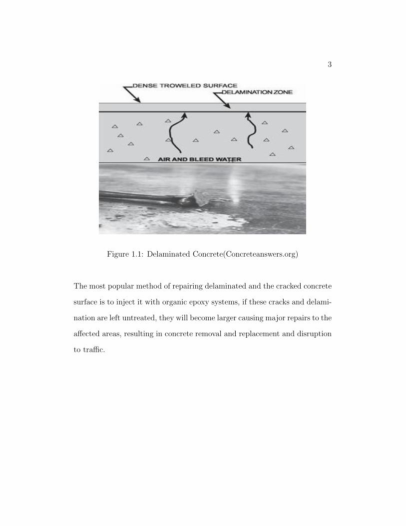
When fresh concrete is placed and compacted, the solids (cement and aggre-
gate) settle. This natural settlement causes excess mix water and entrapped
air to be displaced (called bleeding), and the lighter materials migrate toward
the surface. If finishing operations start prematurely and close or seal the
surface before bleeding is completed, air and or water are trapped under the
dense surface mortar. As concrete hardens, subsurface voids develop where
the water or air is trapped. These voids create weakened zones right below
the surface and are also referred to as delaminations.

2
Restrained shrinkage cracking occurs when concrete is prevented from making
volumetric changes by a source of restraint, either internal or external. The
primary cause of drying shrinkage is the loss of adsorbed water, though the
causes of the water loss for creep and drying shrinkage are radically different.
For drying shrinkage, the driving force behind the water loss is the relative
humidity. Restrained shrinkage induces tensile stresses in concrete
With the presence of cracks in concrete infrastructure for example bridge
decks, water, sulfates, chlorides, and other potentially corrosive agents are
able to permeate to the interior of the bridge deck. These agents cause
further delamination and deterioration in the form of even larger cracks,
spalling, potholes, and eventually a loss of cross section of the bridge deck or
reinforcing steel, which ultimately leads to an unsafe bridge.
3
Figure 1.1: Delaminated Concrete(Concreteanswers.org)
The most popular method of repairing delaminated and the cracked concrete
surface is to inject it with organic epoxy systems, if these cracks and delami-
nation are left untreated, they will become larger causing major repairs to the
affected areas, resulting in concrete removal and replacement and disruption
to traffic.
4
1.1 Epoxy Systems
The first epoxies were designed both in America by Dr. S. O Greenlee and
in Switzerland by Dr. Pierre Castan around 1935 (Epoxy Chemicals, Inc.
2013). The basic components of a 2- part epoxy have not changed since they
were first formulated in the 1930s. The 2-part epoxy consists of a petroleum
based resin and hardener or curative. The reaction is usually rapid and highly
exothermic meaning excessive heat is produced when the resin and hardener
are mixed in large quantities. The practice of repairing cracked concrete by
epoxy injection had become popular by 1960 and the American Concrete
Institute (ACI) published a method for its use (ACI Committee 403 1962).
In 1980 Kansas DOT investigated how long would the repair of bridge decks
with epoxy actually last before the deck would have to be replaced (Strat-
ton and Smith 1988). Four delaminated bridges were epoxy injected and
compared to non injected bridges so that information on delamination repair
durability and the frequency of repair could be collected. It was concluded
that due to the organic nature of the resin and its susceptibility to break-
down by solvents and because the resin grows increasingly brittle over time,
the injection repairs have to be done every 5 years on an average.
Also another study was conducted by Kansas DOT (1974) on how to choose
an epoxy which would be suitable for the repairs. Early epoxy choices were
arbitrary and subject to local availability. This initial epoxy also featured a
higher viscosity, meaning pressures were greater on the original equipment.
5
Once an analytical survey had been completed, it was found that a lower vis-
cosity epoxy was necessary to allow an effective repair solution. The Kansas
DOT studied types of epoxy and gave an outline of the suitable feature set
required for successful epoxy injection (Stratton and McCollom 1974,Connor
1979). Six epoxy systems were targeted to determine acceptable features.
The following distributers were used: Kimmel Engineering Company (KR52-
2 resin and KH-78 hardener), Sinmast of America, INC. (Sinmast Injection
Resin), Adhesive Engineering Company (Concresive 1050-15), and the other
three available from Sika Chemical Corporation (Colma Fix LV, Sikastix 37,
and Sikadur Hi-Mod).
However, the epoxy available from Adhesive Engineering Company was not
tested since the manufacturer limited usage to company trained and licensed
technicians. In addition, early on it was discovered that the Kimmel En-
gineering Company supplied epoxy could be diluted in contact with moist
conditions. Researchers had noted that water could be displaced from the
delaminations during injection so the epoxy should be water-resistant.
The analytical research indicated that the maximum room temperature vis-
cosity should be about 30 poise. The range of the tested epoxies was between
3 and 17 poise. The manufacturer low temperature curing requirements
varied but the lowest was the epoxy manufactured by Sinmast at 33F and
Sikadur Hi-Mod at 40F. All other systems minimum temperature was at
about 60F. It was noted that the average low temperature in Kansas often
6
dipped below 60F at night. The remaining epoxies were tested for bond and
durability against wetting and saline solutions by the use of flexural tests.
These tests involved gluing concrete together and testing in flexure. In the
durability tests, the specimens were soaked in water prior to repair and then
kept in water during the epoxy curing. In all the dry bond cases the break
location was located in the concrete except for the Sika Colma Fix LV which
failed in the bond between the concrete and the epoxy. In the wetting tests,
none of the epoxies survived 100% of the test. The Sikadur Hi Mod had
the best performance with 75% concrete failure and the Sinmast followed
with 66% concrete failure. The rest of the failure was in epoxy debonding.
The Sinmast manufactured epoxy was recommended however because of its
overall performance including low application temperature and viscosity.
A discussion on epoxy systems wouldn’t be complete without discussing the
way to transport the material to the delaminated zone. Initially a drill bit
was used for reaching the delaminated zone. Fig 1.2 shows a modified drill
bit which was developed by Kansas DOT, and is still commonly used.
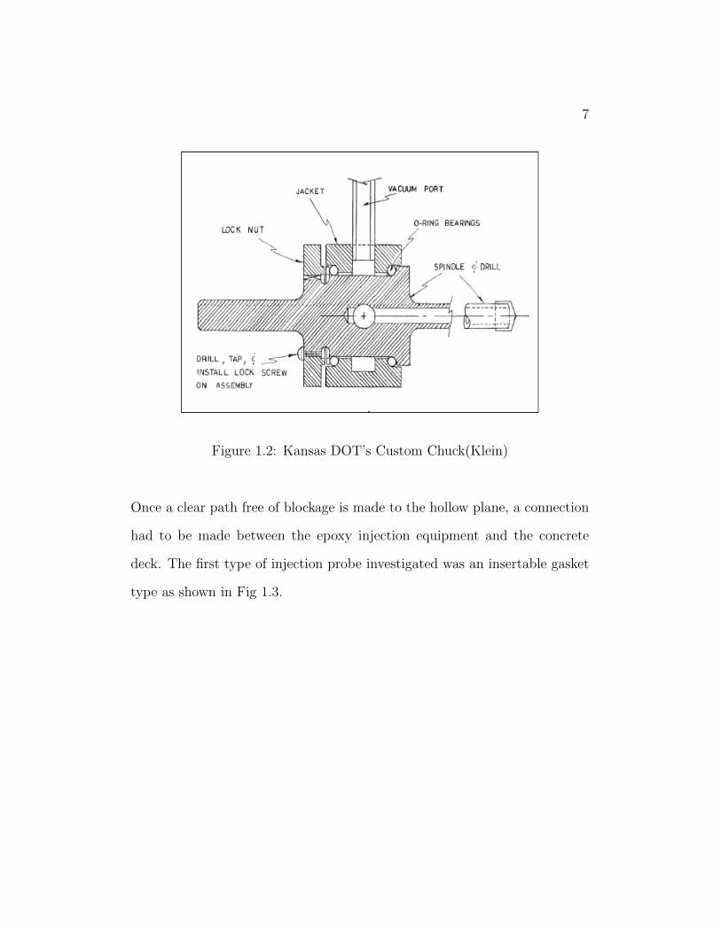
7
Figure 1.2: Kansas DOT’s Custom Chuck(Klein)
Once a clear path free of blockage is made to the hollow plane, a connection
had to be made between the epoxy injection equipment and the concrete
deck. The first type of injection probe investigated was an insertable gasket
type as shown in Fig 1.3.

8
Figure 1.3: Insertable Gasket Type Injection Probe(Klein)
Figure 1.4: Surface Mounted Type Injection Probe(Klein)
The second type of injection probe still featured an insertable probe, but this

9
time, the gasket was surface mounted and held in place by the downward force
of the technician who is operating the probe.
While the internal gasket type could withstand greater pressure and could
remain in position without assistance during injection, it required a mini-
mum depth of insertion to form an effective seal. In addition, the gasket
took more time to replace since it involved removing the injection tip. The
surface gasket type could resist leakage as long as the operator is using the
equipment properly and a lower viscosity epoxy is used, however, if the sur-
face was uneven, the seal could leak. The surface gasket type is prone to
cause operator fatigue though it allowed for quick gasket replacements and
quick injection set-up times.
Epoxy injection is so widely used because it can be used to seal off delami-
nations and cracks through the use of relatively inexpensive equipment and
does not require a large labor force. Because of this, epoxy injection has be-
come a cheaper repair alternative over jack-hammering out the affected area
and replacing with fresh concrete. This allowed for less cost in man-hours
and reduced lane closures since the areas repaired would not have to be shut
down during the curing of the new concrete.
10
1.2 Inorganic Systems
In the 1970s a French scientist, Joseph Davidovits, developed a new class of
inorganic plastics in response to several fire outbreaks in France (Davidovits
1979). The material that he found was a certain group of inorganic min-
eral compositions that shared similar hydrothermal conditions which con-
trol the synthesis of organic phenolic plastics, and of mineral feldpathoids
and zeolites. Both syntheses required a high pH values, concentrated al-
kali,atmospheric pressure and thermoset at temperatures below 300F.
The result of this research was an entirely new family of materials that
were given the name Geopolymer due of the geologic origin and how the
materials share properties with other naturally occurring minerals such as
feldspathoids, feldspars, and zeolites. These properties include thermal sta-
bility, smooth surfaces, hardness, weather resistant and high temperature
resistant up to over 2000F. Unlike the naturally occurring minerals, the
Geopolymers are polymers meaning they can be transformed, tooled, and
molded. They are created in a similar manner to thermosetting organic
resins and cement by poly condensation. The inorganic polymer can be for-
mulated with or without the use of additional performance enhancing fillers
or reinforcement. Applications of the material are found in automobile and
aerospace industries, civil engineering and plastics/ceramics.
The terminology for the division of Geopolymers based on alumino-silicates
is polysialate. Sialate is the acronym for silicon-oxo-aluminate of Na, K, Ca,

11
Li. The structure of the sialate is composed of SiO4 and AlO4 tetrahedrals
linked by the shared oxygen. In the case of potassium alumino-silicates, the
positive ion K+ is present to balance the negative charge of the Al3+ in the
IV-fold coordination. The chemical formula of the potassium polysialate is
Kn(-(SiO2)z - AlO2)n.H2O
where n is the degree of polycondensation and z is 1, 2, or 3. Polysialates
are characterized as chain or ring polymers and in the case of the potas-
sium alumino-silicate the resin hardens to a amorphous solid. The empirical
formula of the potassium polysialate is Si32O99H24K7Al. Elemental compo-
sition, x-ray diffraction, and Si magic angle spinning nuclear magnetic reso-
nance spectroscopy (Si MAS-NMR) have been used to create a representative
structure of the cured inorganic material shown in Figure 1.5 (Davidovits
1991).
Figure 1.5: Chemical Structure Of Potassium Polysialate(Davidovits)
12
The properties of the inorganic polymer have been previously tested as a
part of a long term research study done at Rutgers University under the
guidance of Dr. P. N. Balaguru and in partnership with the Federal Aviation
Administration and the Connecticut Department of Transportation. The
results came largely from the dissertations of Andrew J. Foden(1999) and
Ronald J. Garon (2000) and Matthew Klein (2013).
The properties of the inorganic polymer as shown in Table 1. were determined
by conducting the following tests :
Tension: Tensile strength was determined based on ASTM C496 Standard
Test Method for Splitting Tensile Strength of Cylindrical Concrete Speci-
mens (ASTM C496 2011).
Compression, Strain, and Modulus of Elasticity: Compression strength was
performed using ASTM D695 Standard Test Method for Compressive Prop-
erties of Rigid Plastics (ASTM D695 2010).
The dynamic modulus test was performed by measuring the compressive
wave velocity in a sample. The dynamic shear modulus was found using the
methods given by ASTM D4015 Standard Test Methods for Modulus and
Damping of Soils by Resonant-Column Method (ASTM D4015 2007).
Surface Energy:The strain capacity and surface energy tests were performed
using a technique by Deteresa et al, developed for determination of Kevler
fiber properties (Deteresa et al 1984).
Flexural Strength: The tests for flexural strength, flexural modulus and fail-
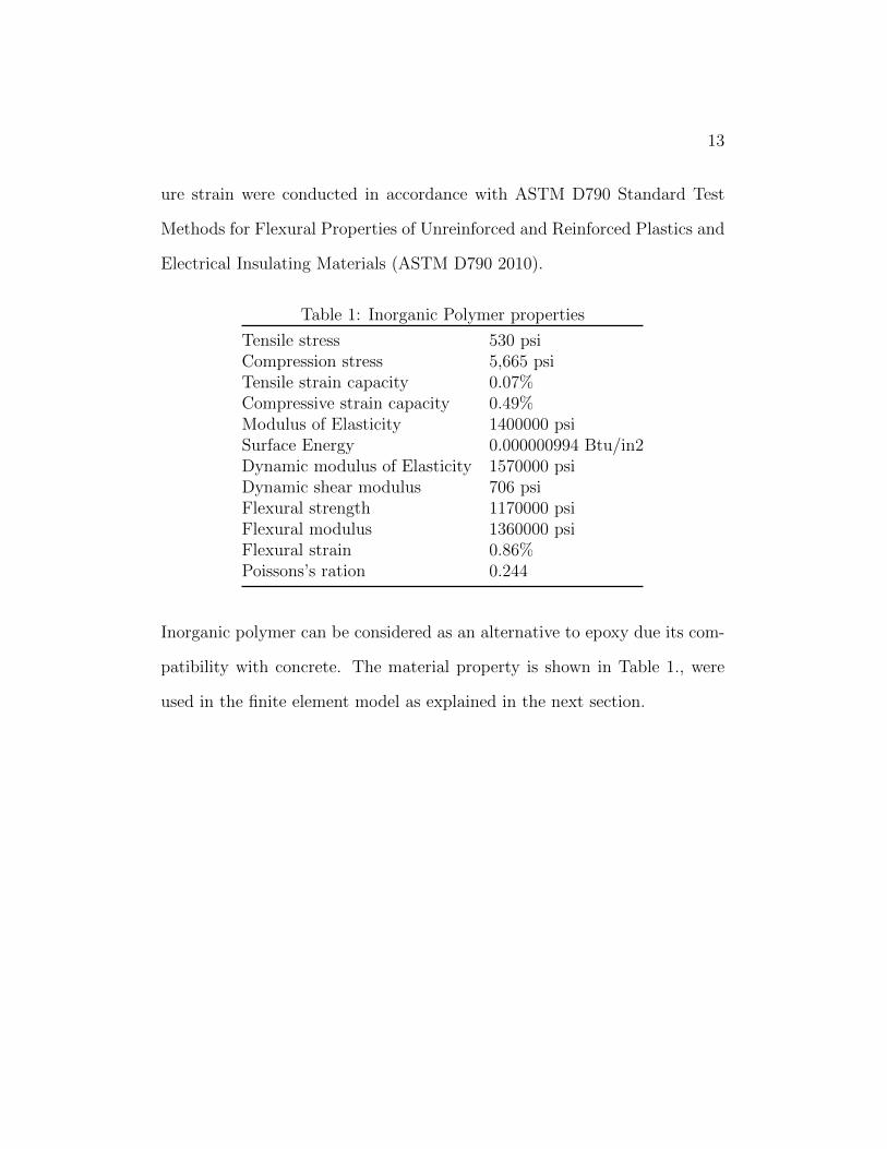
13
ure strain were conducted in accordance with ASTM D790 Standard Test
Methods for Flexural Properties of Unreinforced and Reinforced Plastics and
Electrical Insulating Materials (ASTM D790 2010).
Table 1: Inorganic Polymer properties
Tensile stress 530 psiCompression stress 5,665 psiTensile strain capacity 0.07%Compressive strain capacity 0.49%Modulus of Elasticity 1400000 psiSurface Energy 0.000000994 Btu/in2Dynamic modulus of Elasticity 1570000 psiDynamic shear modulus 706 psiFlexural strength 1170000 psiFlexural modulus 1360000 psiFlexural strain 0.86%Poissons’s ration 0.244
Inorganic polymer can be considered as an alternative to epoxy due its com-
patibility with concrete. The material property is shown in Table 1., were
used in the finite element model as explained in the next section.
14
1.3 Finite Element Based Approach
Typically, the behavior of reinforced concrete beams is studied by full-scale
experimental investigations. Response quantities such as deflections and in-
ternal stress or strain distributions within the beam are compared to the-
oretical calculations.Finite element analysis can also be used to model the
behavior numerically to confirm these calculations, as well as to provide a
valuable supplement to the laboratory investigations, particularly in para-
metric studies. Finite element analysis, as used in structural engineering,
determines the overall behavior of a structure by dividing it into a number
of simple elements, each of which has well-defined mechanical and physical
properties.
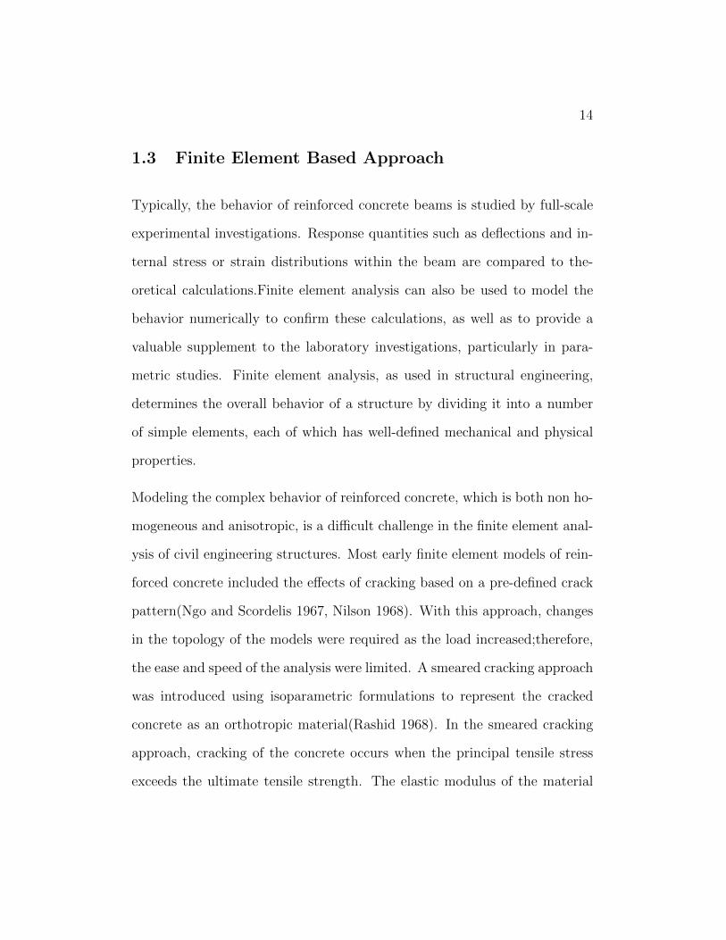
Modeling the complex behavior of reinforced concrete, which is both non ho-
mogeneous and anisotropic, is a difficult challenge in the finite element anal-
ysis of civil engineering structures. Most early finite element models of rein-
forced concrete included the effects of cracking based on a pre-defined crack
pattern(Ngo and Scordelis 1967, Nilson 1968). With this approach, changes
in the topology of the models were required as the load increased;therefore,
the ease and speed of the analysis were limited. A smeared cracking approach
was introduced using isoparametric formulations to represent the cracked
concrete as an orthotropic material(Rashid 1968). In the smeared cracking
approach, cracking of the concrete occurs when the principal tensile stress
exceeds the ultimate tensile strength. The elastic modulus of the material

15
is then assumed to be zero in the direction parallel to the principal tensile
stress direction(Suidan and Schnobrich 1973).
In recent years, however, the use of finite element analysis has increased due
to progressing knowledge and capabilities of computer software and hard-
ware. It has now become the method of choice to analyze concrete structural
components. The use of computer software to model these elements is much
faster, and extremely cost-effective. Data obtained from a finite element
analysis package is not useful unless the necessary steps are taken to under-
stand what is happening within the model that is created using the software.
Also, executing the necessary checks along the way is key to make sure that
what is being output by the computer software is valid. By understanding
the use of finite element packages, more efficient and better analyses can be
made to fully understand the response of individual structural components
and their contribution to a structure as a whole
This thesis is a study of reinforced concrete beams and slabs repaired with
inorganic polymer and epoxy using finite element analysis to understand the
response of repaired reinforced concrete structures when loaded till failure.

16
2 Model description and Analytical investi-
gation
2.1 General
As mentioned, the behavior of reinforced concrete beams is usually studied
by full-scale experimental investigations, in this thesis we study the behavior
of reinforced concrete beams using finite element analysis. The experimental
work done by klien(klein 2013) on experimental investigation of reinforced
concrete beams repaired with inorganic polymer and epoxy is used as a ref-
erence and comparisons are made between the finite element approach and
experimental investigations. The load displacement response from the finite
element analysis was compared to the experimental.
A literature review was conducted on which FEA software to be used to
model the behavior of reinforced concrete. ANSYS 14.5 was selected because
of its ability to model concrete elements. In this study, the reinforced con-
crete model was loaded until failure. ANSYS employs the ”Newton-Raphson”
approach to solve nonlinear problems. In this approach, the load is subdi-
vided into a series of load increments. The load increments can be applied
over several load steps. Figure 2.1 illustrates the use of Newton-Raphson
equilibrium iterations in a single DOF nonlinear analysis.

17
Figure 2.1: Newton-Raphson Iterative Solution
Before each solution, the Newton-Raphson method evaluates the out-of-
balance load vector, which is the difference between the restoring forces (the
loads corresponding to the element stresses) and the applied loads. The pro-
gram then performs a linear solution, using the out-of-balance loads, and
checks for convergence. If convergence criteria are not satisfied, the out-of-
balance load vector is re-evaluated, the stiffness matrix is updated, and a
new solution is obtained. This iterative procedure continues until the prob-
lem converges.
2.2 FE Modeling Of Steel Reinforcement
Tavarez (2001) discusses three techniques that exist to model steel reinforce-
ment in finite element models for reinforced concrete (Figure 2.2): the dis-
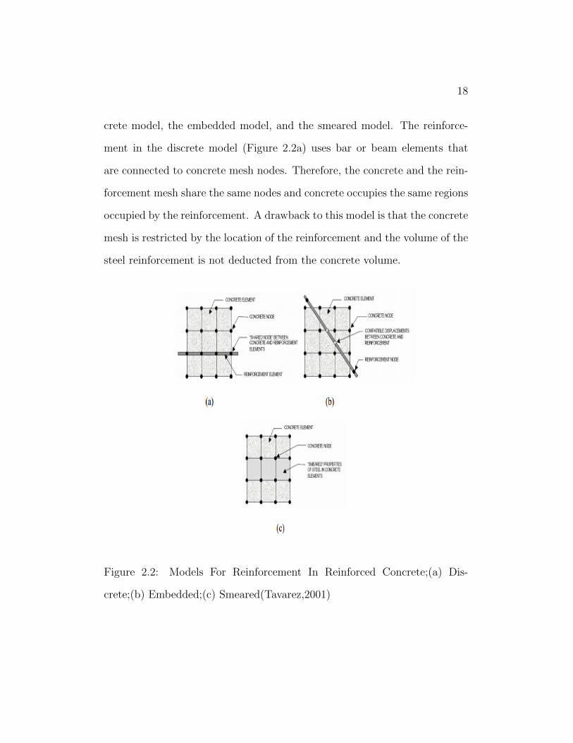
18
crete model, the embedded model, and the smeared model. The reinforce-
ment in the discrete model (Figure 2.2a) uses bar or beam elements that
are connected to concrete mesh nodes. Therefore, the concrete and the rein-
forcement mesh share the same nodes and concrete occupies the same regions
occupied by the reinforcement. A drawback to this model is that the concrete
mesh is restricted by the location of the reinforcement and the volume of the
steel reinforcement is not deducted from the concrete volume.
Figure 2.2: Models For Reinforcement In Reinforced Concrete;(a) Dis-
crete;(b) Embedded;(c) Smeared(Tavarez,2001)
19
The embedded model (Figure 2.2b) overcomes the concrete mesh restrictions
because the stiffness of the reinforcing steel is evaluated separately from the
concrete elements. The model is built in a way that keeps reinforcing steel
displacements compatible with the surrounding concrete elements. When
reinforcement is complex, this model is very advantageous. However, this
model increases the number of nodes and degrees of freedom in the model,
therefore, increasing the run time and computational cost.
The smeared model (Figure 2.2c) assumes that reinforcement is uniformly
spread throughout the concrete elements in a defined region of the FE mesh.
This approach is used for large-scale models where the reinforcement does
not significantly contribute to the overall response of the structure. Fanning
(2001)and Wolanski(2004) modeled the response of the reinforcement using
the discrete model and the smeared model for reinforced concrete beams. It
was found that the best modeling strategy was to use the discrete model
when modeling reinforcement.
20
2.3 Element selection
2.3.1 SOLID 65
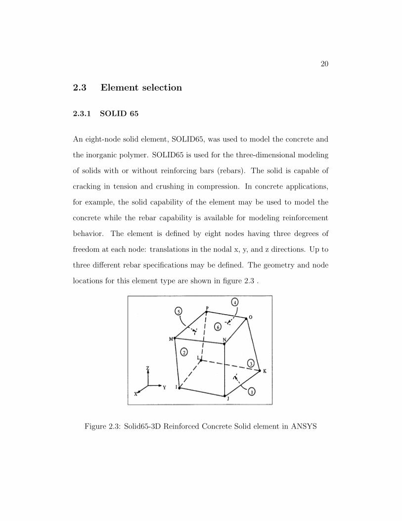
An eight-node solid element, SOLID65, was used to model the concrete and
the inorganic polymer. SOLID65 is used for the three-dimensional modeling
of solids with or without reinforcing bars (rebars). The solid is capable of
cracking in tension and crushing in compression. In concrete applications,
for example, the solid capability of the element may be used to model the
concrete while the rebar capability is available for modeling reinforcement
behavior. The element is defined by eight nodes having three degrees of
freedom at each node: translations in the nodal x, y, and z directions. Up to
three different rebar specifications may be defined. The geometry and node
locations for this element type are shown in figure 2.3 .
Figure 2.3: Solid65-3D Reinforced Concrete Solid element in ANSYS
21
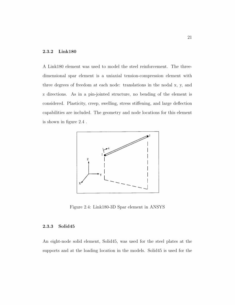
2.3.2 Link180
A Link180 element was used to model the steel reinforcement. The three-
dimensional spar element is a uniaxial tension-compression element with
three degrees of freedom at each node: translations in the nodal x, y, and
z directions. As in a pin-jointed structure, no bending of the element is
considered. Plasticity, creep, swelling, stress stiffening, and large deflection
capabilities are included. The geometry and node locations for this element
is shown in figure 2.4 .
Figure 2.4: Link180-3D Spar element in ANSYS
2.3.3 Solid45
An eight-node solid element, Solid45, was used for the steel plates at the
supports and at the loading location in the models. Solid45 is used for the

22
three-dimensional modeling of solid structures. The element is defined by
eight nodes having three degrees of freedom at each node: translations in
the nodal x, y, and z directions. The element has plasticity, creep, stress
stiffening, large deflection, and large strain capabilities. The geometry and
node locations for this element type are shown in figure 2.5 .
Figure 2.5: Solid45-3D Solid element in ANSYS
2.4 Real Constants
The real constants for concrete element and steel element are shown in Table
2. Note that individual elements contain different real constants. No real
constant set exists for the element Solid45 .
Real Constant Set 1 was used for the element Solid65 element. It requires
real constants for rebar assuming a smeared model. Values can be entered
for Material Number, Volume Ratio, and Orientation Angles. The material
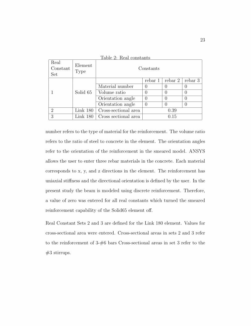
23
Table 2: Real constantsRealConstantSet
ElementType
Constants
1 Solid 65
rebar 1 rebar 2 rebar 3Material number 0 0 0Volume ratio 0 0 0Orientation angle 0 0 0Orientation angle 0 0 0
2 Link 180 Cross-sectional area 0.393 Link 180 Cross sectional area 0.15
number refers to the type of material for the reinforcement. The volume ratio
refers to the ratio of steel to concrete in the element. The orientation angles
refer to the orientation of the reinforcement in the smeared model. ANSYS
allows the user to enter three rebar materials in the concrete. Each material
corresponds to x, y, and z directions in the element. The reinforcement has
uniaxial stiffness and the directional orientation is defined by the user. In the
present study the beam is modeled using discrete reinforcement. Therefore,
a value of zero was entered for all real constants which turned the smeared
reinforcement capability of the Solid65 element off.
Real Constant Sets 2 and 3 are defined for the Link 180 element. Values for
cross-sectional area were entered. Cross-sectional areas in sets 2 and 3 refer
to the reinforcement of 3-#6 bars Cross-sectional areas in set 3 refer to the
#3 stirrups.
24
2.5 Material Properties
2.5.1 Concrete
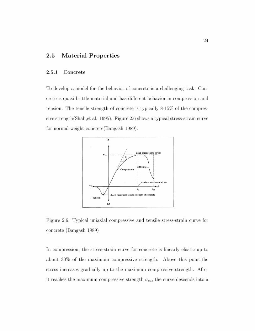
To develop a model for the behavior of concrete is a challenging task. Con-
crete is quasi-brittle material and has different behavior in compression and
tension. The tensile strength of concrete is typically 8-15% of the compres-
sive strength(Shah,et al. 1995). Figure 2.6 shows a typical stress-strain curve
for normal weight concrete(Bangash 1989).
Figure 2.6: Typical uniaxial compressive and tensile stress-strain curve for
concrete (Bangash 1989)
In compression, the stress-strain curve for concrete is linearly elastic up to
about 30% of the maximum compressive strength. Above this point,the
stress increases gradually up to the maximum compressive strength. After
it reaches the maximum compressive strength σcu, the curve descends into a
25
softening region, and eventually crushing failure occurs at an ultimate strain
εcu. In tension, the stress-strain curve for concrete is approximately linearly
elastic up to the maximum tensile strength. After this point, the concrete
cracks and the strength decreases gradually to zero (Bangash 1989).
For concrete, ANSYS requires the following input data for material proper-
ties.
Elastic modulus (Ec).
Ultimate uniaxial compressive strength(f’c).
Ultimate uniaxial tensile strength(modulus of rupture,fr).
Poisson’s ratio (ν).
Shear transfer coefficient(βt).
Compressive uniaxial stress-strain relationship for concrete.
The elastic modulus of concrete is taken from the experimental investigation
conducted by (Klein 2013). From elastic modulus , the ultimate concrete
compressive and tensile strength were calculated by Equations 2.4.1 and 2.4.2
(ACI 318,1999).
f ′c = (
Ec57000
)2 (2.5.1)
fr = 7.5√f ′c (2.5.2)
where Ec,f′candfr are in psi.
Poisson;s ratio was taken an 0.18 in the FE model. The shear transfer
coefficient,βt, represents conditions of the crack face. The value of βt ranges
from 0.0 to 1.0, with 0.0 representing a smooth crack(complete loss of shear)
26
and 1.0 representing a rough crack(no loss of shear). The value of βt used
in many studies of reinforced concrete structures, however, varied between
0.05 and 0.25(Bangash 1989,Husye.et al 1994,Kachlakev and Miller 2000). A
value of 0.3 was selected in this study keeping solution convergence in mind.
Uniaxial Stress-Strain Relationship For Concrete The ANSYS pro-
gram requires the uniaxial stress-strain relationship for concrete in compres-
sion. Numerical expressions(Desayi and krishnan 1964) from equations 2.4.3
and 2.4.4,were used along with equation 2.4.5(Gere and Timoshenko 1997)
to construct the uniaxial compressive stress-strain curve for concrete in this
study.
f =Ecε
1 + ( εεo
)2(2.5.3)
εo =2f ′
c
Ec(2.5.4)
Ec =f
ε(2.5.5)
where:
f=stress at any strain ε,psi
ε = strain at stress f
εo = strain at the ultimate compressive strength f ′c
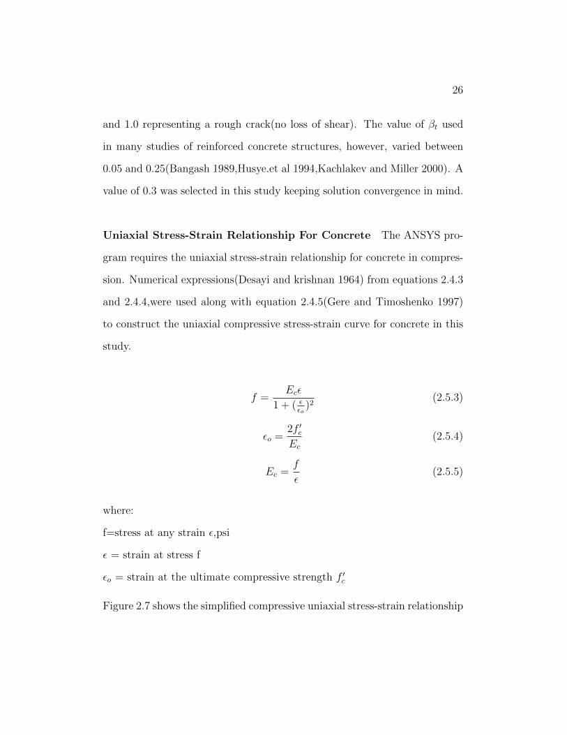
Figure 2.7 shows the simplified compressive uniaxial stress-strain relationship
27
that was used in this study. In this study, an assumption was made of
perfectly plastic behavior after the last data point.
Figure 2.7: Simplified stress-strain model of concrete in compression
Failure Criteria Of Concrete The developed model is capable of pre-
dicting failure of concrete materials for both cracking and crushing failure
modes. The two input strength parameters needed to define the failure sur-
face for the concrete are the ultimate tensile and compressive strengths .
Consequently, a criterion for failure of the concrete due to a multiaxial stress
state can be calculated from these input parameters(William and Warnke
1975).
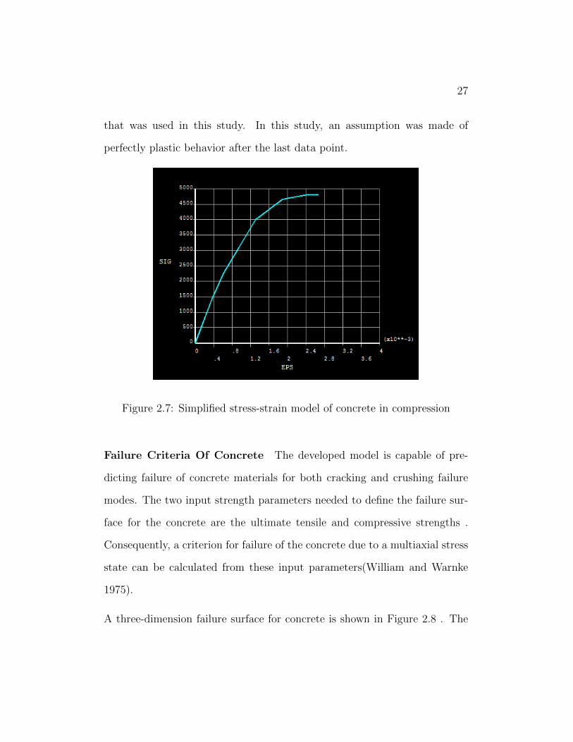
A three-dimension failure surface for concrete is shown in Figure 2.8 . The
28
most significant nonzero principal stresses are in the x and y directions,
represented by σxp and σyp, respectively.Three failure surfaces are shown as
projections on the σxp-σyp plane. The mode of failure is a function of the sign
σzp(principal stress in the z direction). For example, if σxp and σyp are both
negative(compressive) and σzp is slightly positive (tensile), cracking would
be predicted in a direction perpendicular to σzp. However, if σzp is zero or
slightly negative, the material is assumed to crush (ANSYS).
Figure 2.8: 3-D failure surface for concrete in ANSYS (Kachlakev 2000)
In a concrete element, cracking occurs when the principal tensile stress in any
direction lies outside the failure surface. After cracking, the elastic modulus
of the concrete element is set to zero in the direction parallel to the principal
tensile stress direction. Crushing occurs when all principal stresses are com-

29
pressive and lie outside the failure surface;subsequently, the elastic modulus
is set to zero in all directions,and the element effectively disappears(ANSYS).
In this study, it was found that if the crushing capability of the concrete
is turned on, the finite element beam models fail prematurely. Crushing of
the concrete started to develop in elements located directly under the loads.
Subsequently, adjacent concrete elements crushed within several load steps
as well, significantly reducing the local stiffness.
A pure ”compression” failure of concrete is unlikely. In a compression test,
the specimen is subjected to a uniaxial compressive load. Secondary tensile
strains induced by poisson’s effect occur perpendicular to the load. Because
concrete is relatively weak in tension, these stresses actually cause cracking
and the eventual failure (Mindess and Young 1981;Shah,et al.1995,Kachlakev
and Miller 2000). In this study, the crushing capability was turned off and
cracking of the concrete controlled the failure of the finite element models.
2.5.2 Steel Reinforcement and Steel Plates
Steel reinforcement in the experimental beams was constructed with typical
Grade 60 steel reinforcing bars (Klein 2013). The elastic modulus and yield
stress for the steel reinforcement used in the FE were the same material
properties used in the experimental investigation. The steel for the finite
element models was assumed to be an elastic-perfectly plastic material and
identical in tension and compression. A Poisson’s ratio of 0.3 was used for
30
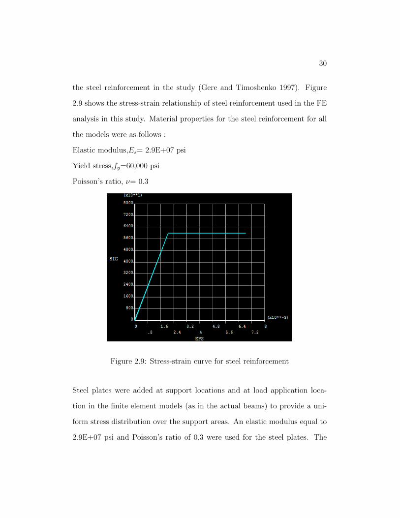
the steel reinforcement in the study (Gere and Timoshenko 1997). Figure
2.9 shows the stress-strain relationship of steel reinforcement used in the FE
analysis in this study. Material properties for the steel reinforcement for all
the models were as follows :
Elastic modulus,Es= 2.9E+07 psi
Yield stress,fy=60,000 psi
Poisson’s ratio, ν= 0.3
Figure 2.9: Stress-strain curve for steel reinforcement
Steel plates were added at support locations and at load application loca-
tion in the finite element models (as in the actual beams) to provide a uni-
form stress distribution over the support areas. An elastic modulus equal to
2.9E+07 psi and Poisson’s ratio of 0.3 were used for the steel plates. The
31
steel plates were assumed to be linear elastic materials.
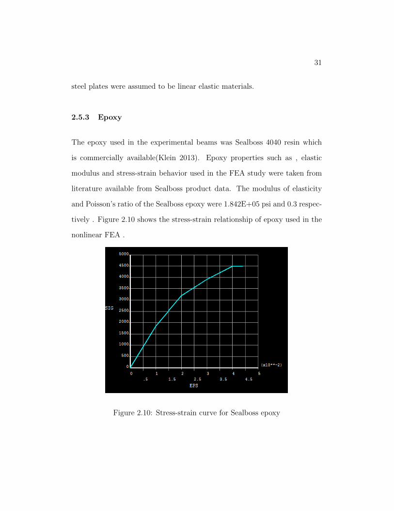
2.5.3 Epoxy
The epoxy used in the experimental beams was Sealboss 4040 resin which
is commercially available(Klein 2013). Epoxy properties such as , elastic
modulus and stress-strain behavior used in the FEA study were taken from
literature available from Sealboss product data. The modulus of elasticity
and Poisson’s ratio of the Sealboss epoxy were 1.842E+05 psi and 0.3 respec-
tively . Figure 2.10 shows the stress-strain relationship of epoxy used in the
nonlinear FEA .
Figure 2.10: Stress-strain curve for Sealboss epoxy
32
2.5.4 Inorganic Polymer
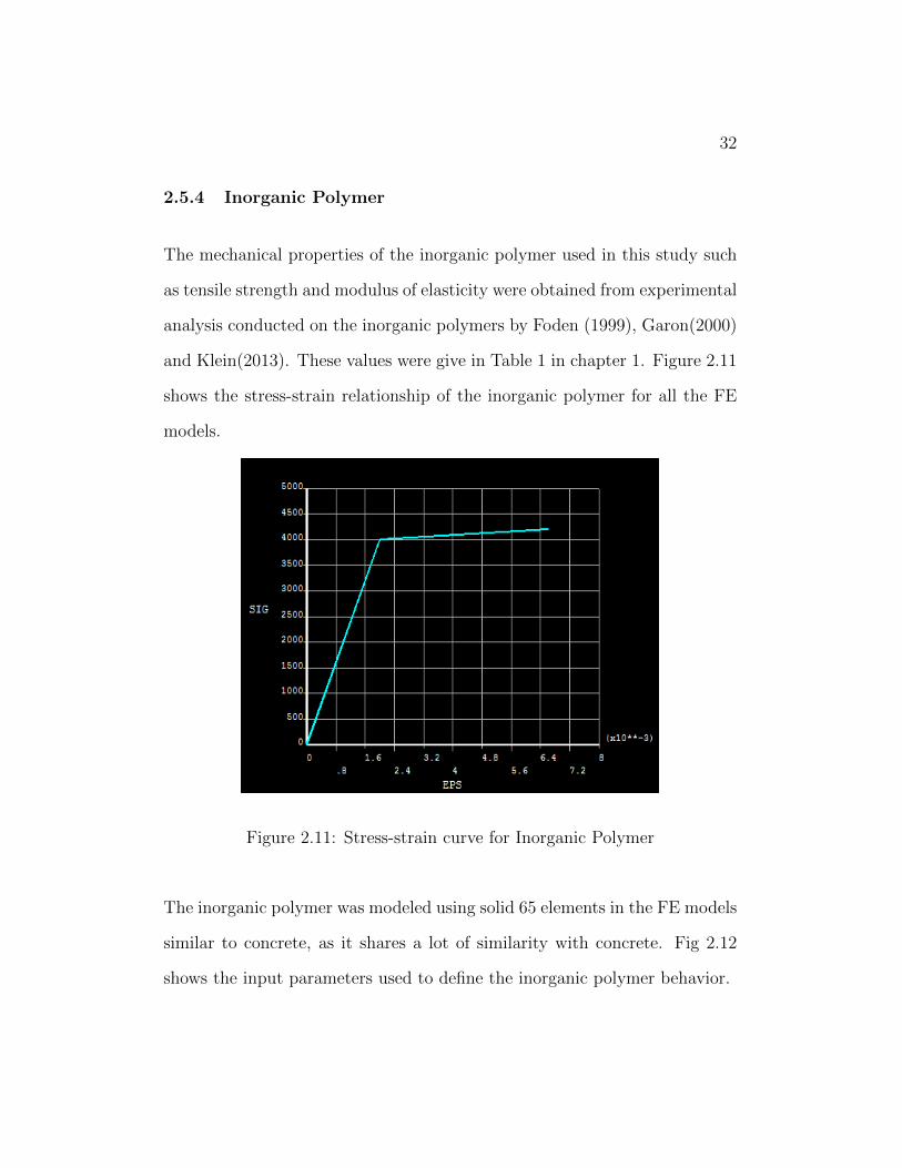
The mechanical properties of the inorganic polymer used in this study such
as tensile strength and modulus of elasticity were obtained from experimental
analysis conducted on the inorganic polymers by Foden (1999), Garon(2000)
and Klein(2013). These values were give in Table 1 in chapter 1. Figure 2.11
shows the stress-strain relationship of the inorganic polymer for all the FE
models.
Figure 2.11: Stress-strain curve for Inorganic Polymer
The inorganic polymer was modeled using solid 65 elements in the FE models
similar to concrete, as it shares a lot of similarity with concrete. Fig 2.12
shows the input parameters used to define the inorganic polymer behavior.
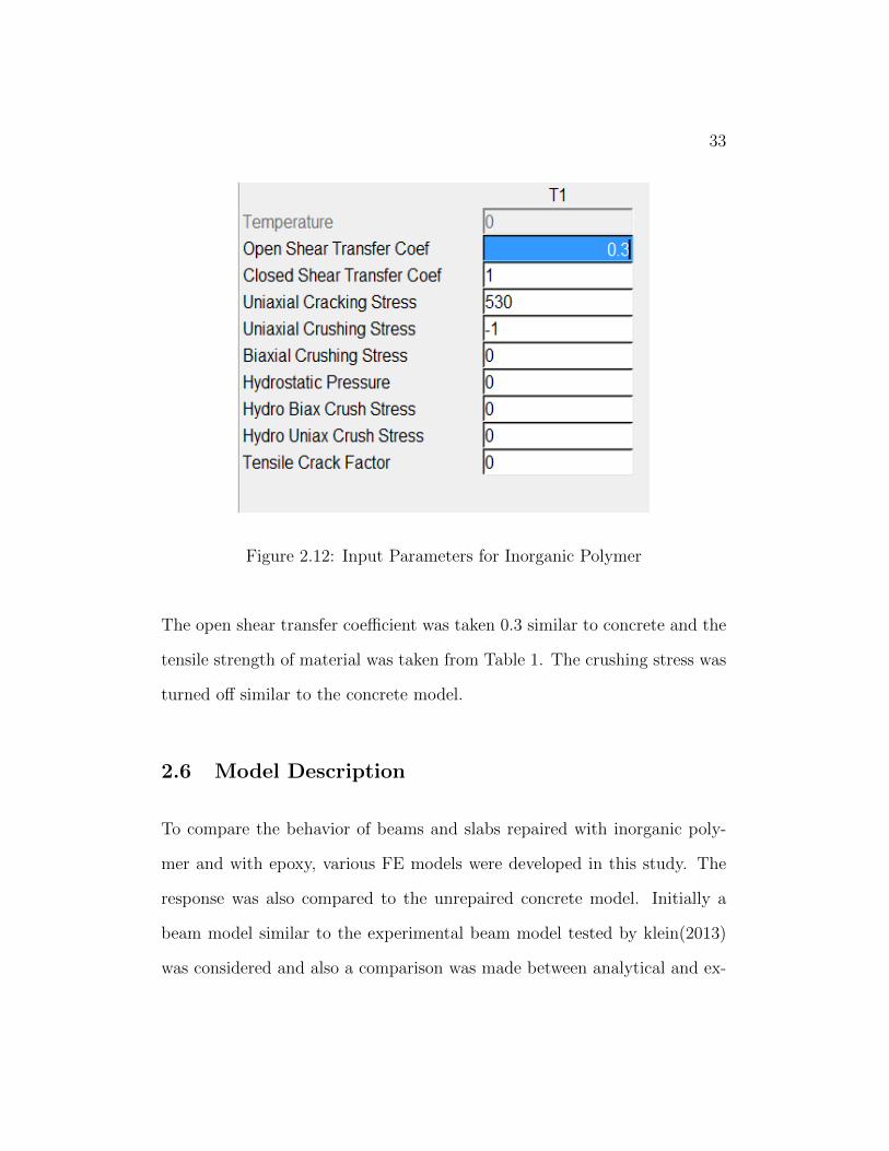
33
Figure 2.12: Input Parameters for Inorganic Polymer
The open shear transfer coefficient was taken 0.3 similar to concrete and the
tensile strength of material was taken from Table 1. The crushing stress was
turned off similar to the concrete model.
2.6 Model Description
To compare the behavior of beams and slabs repaired with inorganic poly-
mer and with epoxy, various FE models were developed in this study. The
response was also compared to the unrepaired concrete model. Initially a
beam model similar to the experimental beam model tested by klein(2013)
was considered and also a comparison was made between analytical and ex-
34
perimental investigations in the future chapters. The thickness of the notch
to be repaired with polymers was varied to see the effect of the size of the
void on the behavior of structure. Lastly a slab model was modeled to see
the behavior of the slab repaired in multiple locations with the polymer. The
descriptions of each model is as follows.
2.6.1 Beam Models I and II
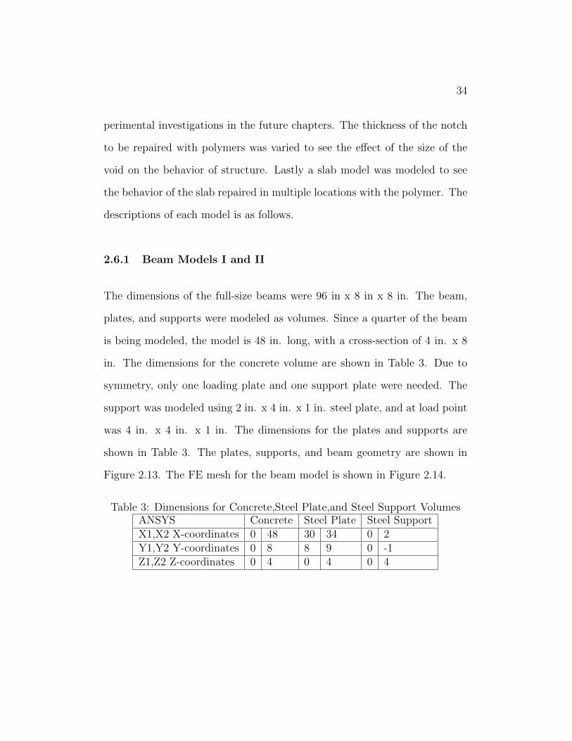
The dimensions of the full-size beams were 96 in x 8 in x 8 in. The beam,
plates, and supports were modeled as volumes. Since a quarter of the beam
is being modeled, the model is 48 in. long, with a cross-section of 4 in. x 8
in. The dimensions for the concrete volume are shown in Table 3. Due to
symmetry, only one loading plate and one support plate were needed. The
support was modeled using 2 in. x 4 in. x 1 in. steel plate, and at load point
was 4 in. x 4 in. x 1 in. The dimensions for the plates and supports are
shown in Table 3. The plates, supports, and beam geometry are shown in
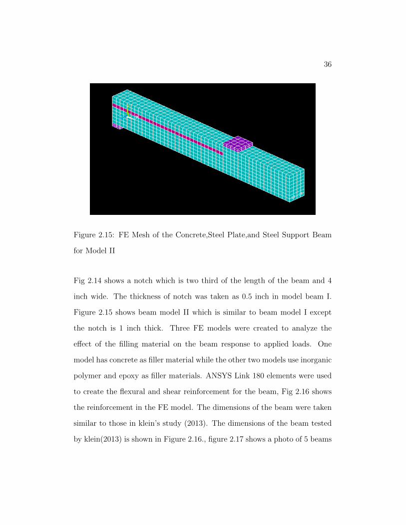
Figure 2.13. The FE mesh for the beam model is shown in Figure 2.14.
Table 3: Dimensions for Concrete,Steel Plate,and Steel Support VolumesANSYS Concrete Steel Plate Steel SupportX1,X2 X-coordinates 0 48 30 34 0 2Y1,Y2 Y-coordinates 0 8 8 9 0 -1Z1,Z2 Z-coordinates 0 4 0 4 0 4
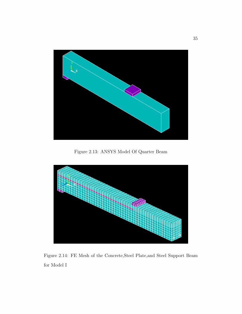
35
Figure 2.13: ANSYS Model Of Quarter Beam
Figure 2.14: FE Mesh of the Concrete,Steel Plate,and Steel Support Beam
for Model I
36
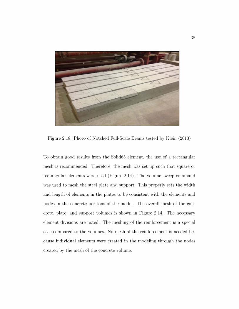
Figure 2.15: FE Mesh of the Concrete,Steel Plate,and Steel Support Beam
for Model II
Fig 2.14 shows a notch which is two third of the length of the beam and 4
inch wide. The thickness of notch was taken as 0.5 inch in model beam I.
Figure 2.15 shows beam model II which is similar to beam model I except
the notch is 1 inch thick. Three FE models were created to analyze the
effect of the filling material on the beam response to applied loads. One
model has concrete as filler material while the other two models use inorganic
polymer and epoxy as filler materials. ANSYS Link 180 elements were used
to create the flexural and shear reinforcement for the beam, Fig 2.16 shows
the reinforcement in the FE model. The dimensions of the beam were taken
similar to those in klein’s study (2013). The dimensions of the beam tested
by klein(2013) is shown in Figure 2.16., figure 2.17 shows a photo of 5 beams

37
tested by klein(2013) with different filler materials.
Figure 2.16: Steel Reinforcement In The FEM Model)
Figure 2.17: Full Scale Beam Dimensions tested by Klein (2013)
38
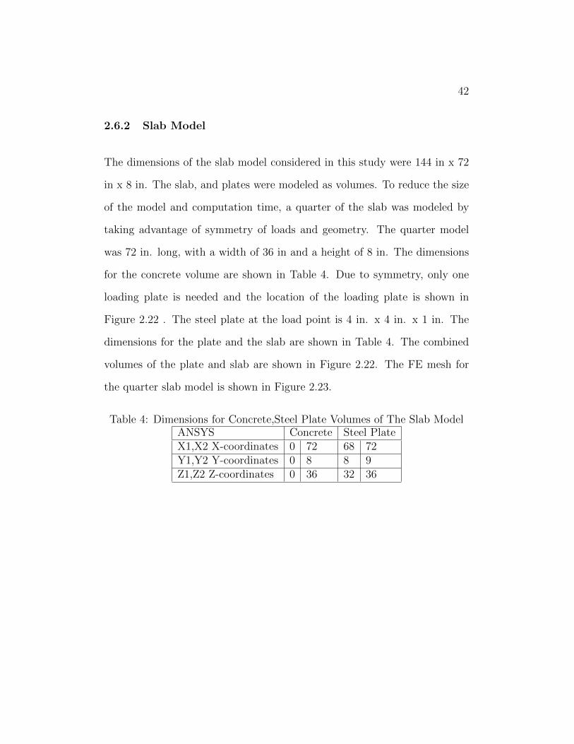
Figure 2.18: Photo of Notched Full-Scale Beams tested by Klein (2013)
To obtain good results from the Solid65 element, the use of a rectangular
mesh is recommended. Therefore, the mesh was set up such that square or
rectangular elements were used (Figure 2.14). The volume sweep command
was used to mesh the steel plate and support. This properly sets the width
and length of elements in the plates to be consistent with the elements and
nodes in the concrete portions of the model. The overall mesh of the con-
crete, plate, and support volumes is shown in Figure 2.14. The necessary
element divisions are noted. The meshing of the reinforcement is a special
case compared to the volumes. No mesh of the reinforcement is needed be-
cause individual elements were created in the modeling through the nodes
created by the mesh of the concrete volume.

39
The command ”merge items” merges separate entities that have the same
location. These items will then be merged into single entities. Caution must
be taken when merging entities in a model that has already been meshed
because the order in which merging occurs is significant. Merging keypoints
before nodes can result in some of the nodes becoming orphaned; that is,
the nodes lose their association with the solid model. The orphaned nodes
can cause certain operations (such as boundary condition transfers, surface
load transfers, and so on) to fail. Care must be taken to always merge in
the order that the entities appear. All precautions were taken to ensure that
everything was merged in the proper order. Also, the lowest number was
retained during merging.
Displacement boundary conditions are needed to constrain the model to get
a unique solution. To ensure that the model acts the same way as the experi-
mental beam, boundary conditions need to be applied at points of symmetry,
and where the supports and loads exist. The symmetry boundary conditions
were set first. The model being used is symmetric about two planes. The
boundary conditions for both planes of symmetry are shown in Figure 2.19.

40
Figure 2.19: Boundary Conditions For Planes Of Symmetry (Top View)
Nodes defining a vertical plane through the beam cross-section centroid de-
fines a plane of symmetry. To model the symmetry, nodes on this plane must
be constrained in the perpendicular direction. These nodes, therefore, have
a degree of freedom constraint UX = 0. Second, all nodes selected at Z =
0 define another plane of symmetry. These nodes were given the constraint
UZ = 0. A single line of nodes on the plate were given constraint in the UX,
UY, and UZ directions, applied as constant values of 0 at the support. By
doing this, the beam will be allowed to rotate at the support. The support
condition is shown in Figure 2.20.

41
Figure 2.20: Boundary Conditions For Support
The force, P, applied at the steel plate is applied across the entire center line
of the plate. The force applied at each node on the plate is one tenth of the
actual force applied. Figure 2.21 illustrates the plate and applied loading
Figure 2.21: Boundary Conditions For Plate For Load Application
42
2.6.2 Slab Model
The dimensions of the slab model considered in this study were 144 in x 72
in x 8 in. The slab, and plates were modeled as volumes. To reduce the size
of the model and computation time, a quarter of the slab was modeled by
taking advantage of symmetry of loads and geometry. The quarter model
was 72 in. long, with a width of 36 in and a height of 8 in. The dimensions
for the concrete volume are shown in Table 4. Due to symmetry, only one
loading plate is needed and the location of the loading plate is shown in
Figure 2.22 . The steel plate at the load point is 4 in. x 4 in. x 1 in. The
dimensions for the plate and the slab are shown in Table 4. The combined
volumes of the plate and slab are shown in Figure 2.22. The FE mesh for
the quarter slab model is shown in Figure 2.23.
Table 4: Dimensions for Concrete,Steel Plate Volumes of The Slab ModelANSYS Concrete Steel PlateX1,X2 X-coordinates 0 72 68 72Y1,Y2 Y-coordinates 0 8 8 9Z1,Z2 Z-coordinates 0 36 32 36

43
Figure 2.22: Volumes Created For ANSYS Quarter Slab Model
Figure 2.23: ANSYS FE mesh for the Quarter Slab Model
44
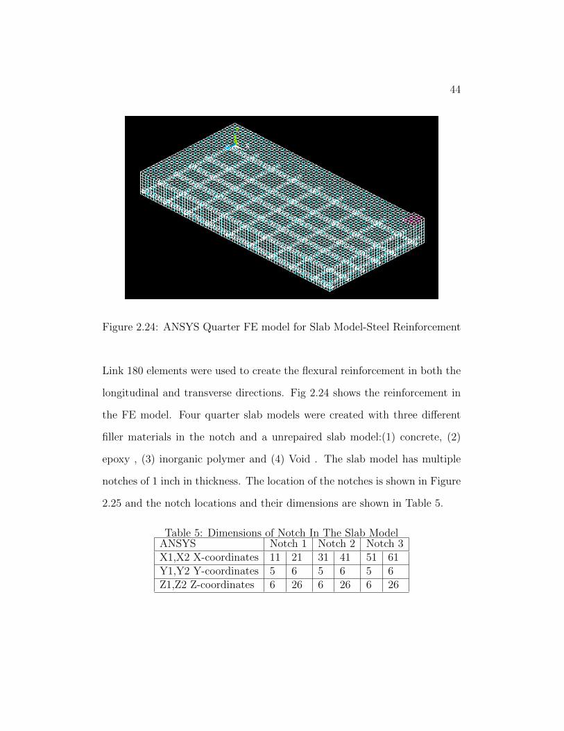
Figure 2.24: ANSYS Quarter FE model for Slab Model-Steel Reinforcement
Link 180 elements were used to create the flexural reinforcement in both the
longitudinal and transverse directions. Fig 2.24 shows the reinforcement in
the FE model. Four quarter slab models were created with three different
filler materials in the notch and a unrepaired slab model:(1) concrete, (2)
epoxy , (3) inorganic polymer and (4) Void . The slab model has multiple
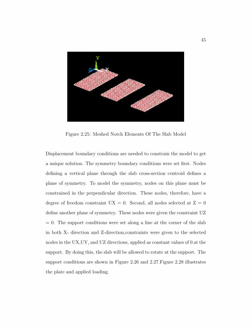
notches of 1 inch in thickness. The location of the notches is shown in Figure
2.25 and the notch locations and their dimensions are shown in Table 5.
Table 5: Dimensions of Notch In The Slab ModelANSYS Notch 1 Notch 2 Notch 3X1,X2 X-coordinates 11 21 31 41 51 61Y1,Y2 Y-coordinates 5 6 5 6 5 6Z1,Z2 Z-coordinates 6 26 6 26 6 26
45
Figure 2.25: Meshed Notch Elements Of The Slab Model
Displacement boundary conditions are needed to constrain the model to get
a unique solution. The symmetry boundary conditions were set first. Nodes
defining a vertical plane through the slab cross-section centroid defines a
plane of symmetry. To model the symmetry, nodes on this plane must be
constrained in the perpendicular direction. These nodes, therefore, have a
degree of freedom constraint UX = 0. Second, all nodes selected at Z = 0
define another plane of symmetry. These nodes were given the constraint UZ
= 0. The support conditions were set along a line at the corner of the slab
in both X- direction and Z-direction,constraints were given to the selected
nodes in the UX,UY, and UZ directions, applied as constant values of 0 at the
support. By doing this, the slab will be allowed to rotate at the support. The
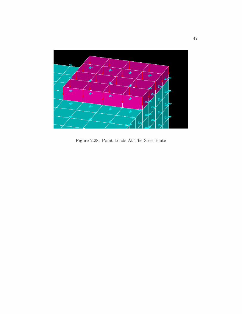
support conditions are shown in Figure 2.26 and 2.27.Figure 2.28 illustrates
the plate and applied loading.
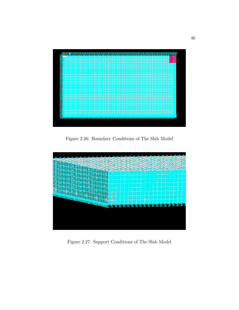
46
Figure 2.26: Boundary Conditions of The Slab Model
Figure 2.27: Support Conditions of The Slab Model
47
Figure 2.28: Point Loads At The Steel Plate
48
3 Analysis Results And Discussion
In the previous chapter we discussed how to set up the model in ANSYS
with regards to material selection, element selection, real constants, geometry
and meshing of the model. In this chapter we shall study how to set up the
parameters for the final analysis model and look into the solution the program
generates. Also a simultaneous discussion is provided on the solution of the
models described in the previous chapter.
The different cases modeled using ANSYS are as follows
Beam Model I
1. Control I (reinforced Concrete Beam )
2. Notched Epoxy Beam I (reinforced concrete beam repaired with epoxy
in the delaminated zone)
3. Notched Inorganic Beam I(reinforced concrete beam repaired with in-
organic polymer in the delaminated zone)
Beam Model II
1. Control II (reinforced concrete beam)
2. Notched Epoxy Beam II (reinforced concrete beam repaired with epoxy
in the delaminated zone)

49
3. Notched Inorganic Beam II (reinforced concrete beam repaired with
inorganic polymer in the delaminated zone)
Slab Model
1. Control Slab(reinforced concrete slab model)
2. Notched Epoxy Slab (reinforced concrete slab repaired in multiple de-
laminated zones with epoxy)
3. Notched Inorganic Slab (reinforced concrete slab repaired in multiple
delaminated zones with inorganic polymer)
4. Notched Slab (reinforced concrete slab with delaminated zones without
any repair)
3.1 Analysis
The FE analysis of the model was set up to examine three different behav-
iors: initial cracking of the beam, yielding of the steel reinforcement, and the
strength limit state of the beam. The Newton-Raphson method of analysis
was used to compute the nonlinear response. The restart command is uti-
lized to continue the run from the last converged sub step with changes in
convergence inputs till the beam completely fails. Below are the input data
that are given for the analysis.
50
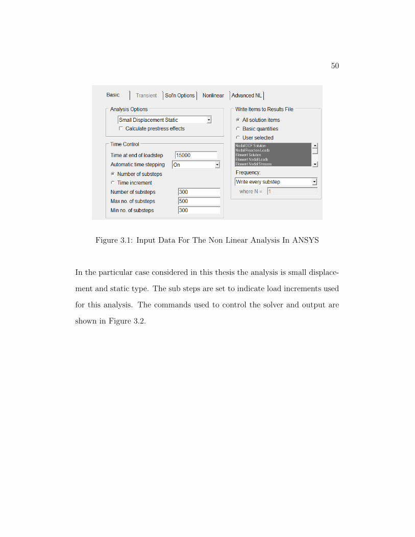
Figure 3.1: Input Data For The Non Linear Analysis In ANSYS
In the particular case considered in this thesis the analysis is small displace-
ment and static type. The sub steps are set to indicate load increments used
for this analysis. The commands used to control the solver and output are
shown in Figure 3.2.

51
Figure 3.2: Solution Controls
The commands used for the nonlinear algorithm and convergence criteria are
shown in Figure 3.3. Values for the nonlinear algorithm were set to defaults.
Figure 3.3: Non Linear Solution Controls

52
Once the beam cracks the force convergence criteria was dropped because of
non convergence, solution was based on displacement convergence criteria.
The displacement tolerance was kept as low as possible to capture the correct
response of the model.
53
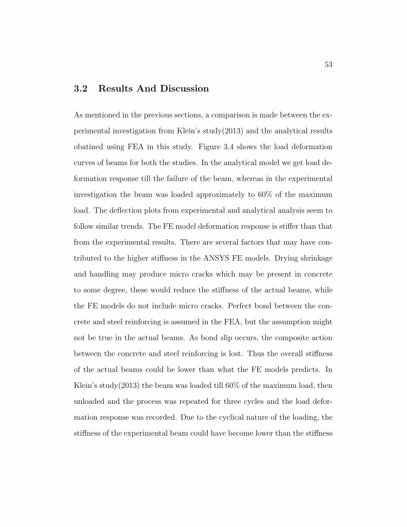
3.2 Results And Discussion
As mentioned in the previous sections, a comparison is made between the ex-
perimental investigation from Klein’s study(2013) and the analytical results
obatined using FEA in this study. Figure 3.4 shows the load deformation
curves of beams for both the studies. In the analytical model we get load de-
formation response till the failure of the beam, whereas in the experimental
investigation the beam was loaded approximately to 60% of the maximum
load. The deflection plots from experimental and analytical analysis seem to
follow similar trends. The FE model deformation response is stiffer than that
from the experimental results. There are several factors that may have con-
tributed to the higher stiffness in the ANSYS FE models. Drying shrinkage
and handling may produce micro cracks which may be present in concrete
to some degree, these would reduce the stiffness of the actual beams, while
the FE models do not include micro cracks. Perfect bond between the con-
crete and steel reinforcing is assumed in the FEA, but the assumption might
not be true in the actual beams. As bond slip occurs, the composite action
between the concrete and steel reinforcing is lost. Thus the overall stiffness
of the actual beams could be lower than what the FE models predicts. In
Klein’s study(2013) the beam was loaded till 60% of the maximum load, then
unloaded and the process was repeated for three cycles and the load defor-
mation response was recorded. Due to the cyclical nature of the loading, the
stiffness of the experimental beam could have become lower than the stiffness
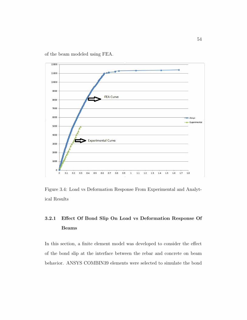
54
of the beam modeled using FEA.
Figure 3.4: Load vs Deformation Response From Experimental and Analyt-
ical Results
3.2.1 Effect Of Bond Slip On Load vs Deformation Response Of
Beams
In this section, a finite element model was developed to consider the effect
of the bond slip at the interface between the rebar and concrete on beam
behavior. ANSYS COMBIN39 elements were selected to simulate the bond

55
and bond slip at the interface between concrete and steel rebar.
COMBIN39 is a unidirectional element with nonlinear generalized force-
deformation capability that can be used in most analyses. The element has
longitudinal or torsional capability in one, two, or three dimensional appli-
cations. The geometry, node locations, and the coordinate system for this
element are shown in Figure 3.5. The element is defined by two node points
and a generalized force-deformation curve. The points on this curve (D1, F1,
etc.) represent force versus relative translation for structural analyses. The
force-deformation curve should be input such that deflections are increasing
from the third (compression) to the first (tension) quadrants. Adjacent de-
formation should not be less than 1E-7 times total input deformation range.
The last input deformation must be positive. Segments tending towards ver-
tical should be avoided. If the force-deformation curve limits are exceeded,
the last defined slope is maintained, and the status remains equal to the last
segment number.
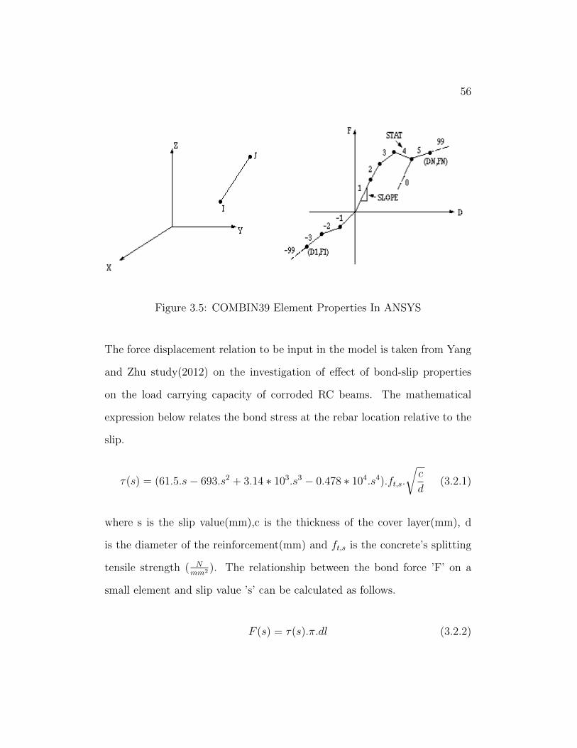
56
Figure 3.5: COMBIN39 Element Properties In ANSYS
The force displacement relation to be input in the model is taken from Yang
and Zhu study(2012) on the investigation of effect of bond-slip properties
on the load carrying capacity of corroded RC beams. The mathematical
expression below relates the bond stress at the rebar location relative to the
slip.
τ(s) = (61.5.s− 693.s2 + 3.14 ∗ 103.s3 − 0.478 ∗ 104.s4).ft,s.
√c
d(3.2.1)
where s is the slip value(mm),c is the thickness of the cover layer(mm), d
is the diameter of the reinforcement(mm) and ft,s is the concrete’s splitting
tensile strength ( Nmm2 ). The relationship between the bond force ’F’ on a
small element and slip value ’s’ can be calculated as follows.
F (s) = τ(s).π.dl (3.2.2)

57
Where d is the diameter of a bar(mm) and l is the distance between two
adjacent springs(mm). From equation 3.2.1 and 3.2.2, the force vs displace-
ment relationship of the spring element in the longitudinal direction can be
obtained.
Figure 3.6: Bond-Slip Force Displacement Plot Input In ANSYS
Figure 3.6 shows the force vs displacement curve for the spring element that
was input in ANSYS in the tension quadrant. For the compression quadrant
the curve is a reflection of the tension curve.
In the FE model, COMBIN39 elements were modeled as zero length springs
at the location where steel and concrete have shared nodes. Two sets of
duplicated nodes were created at locations where steel and concrete have
58
shared nodes previously. Zero length springs were created such that the
steel node is connected to concrete node with a spring . The zero length
spring elements were defined in the longitudinal direction. The new ANSYS
model includes the force displacement relation of the springs defined using the
bond slip equation 3.2.1. the model was analyzed and the load deformation
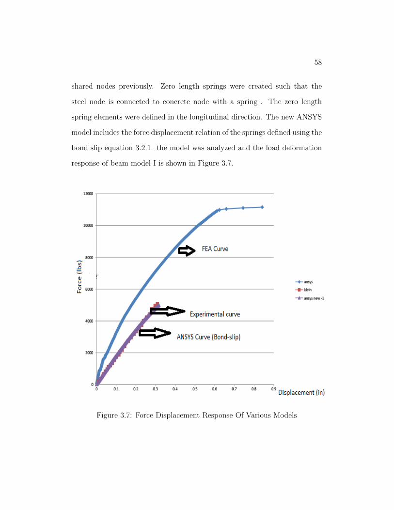
response of beam model I is shown in Figure 3.7.
Figure 3.7: Force Displacement Response Of Various Models
59
Figure 3.7 shows the force deformations response for three cases. In the first
case the FE model developed considers a perfect bond between the rebar and
concrete and because of this assumption we observe the response of the model
to load is stiffer. In the second case, a model was developed to account for
the bond slip in the FE model to be compared with the experimental results
which are shown in the third curve. We observe that the response of the
FE model with bond slip, behaves similar to the experimental results. It
can be said that incorporating the bond slip interaction at the steel concrete
interface could give more accurate response of the structure, but also it should
be noted that the bond slip interaction at the interface is complex to quantify
and the presence of micro cracks due to handling and shrinkage, and also the
cyclical nature of the loading could have caused the higher deformation to
load in the experimental investigation conducted by Klein(2013).
3.2.2 Beam Model I
In this section, results for the analysis of beam model I are discussed. Cracked
patterns of the beam when loaded till failure are shown in Figure 3.5,3.6 and
3.7. A cracking sign represented by a circle appears when a principal tensile
stress exceeds the ultimate tensile strength of the concrete. The cracking
sign appears perpendicular to the direction of the principal stress as seen
in the figures below. Figure 3.5 shows a side face of a quarter beam model
of control I. As shown in figure, at the bottom of the beam at mid span,
60
principal tensile stresses occur mostly in x direction (longitudinally). When
principal stresses exceed the ultimate tensile strength of the concrete, crack-
ing signs appear as circles perpendicular to the principal stresses in the x
direction. Therefore the cracking signs shown in the figure appear as ver-
tical straight lines occurring at the integration points of the concrete solid
elements. These are also referred to as flexural cracks. In the figure below,
cracking signs are observed underneath the loading locations. These cracks
result from tensile strains developed due to poisson’s effect(Kachlakev 2000).
These cracks are referred to as compressive cracks. In the figures below, we
can observe inclined cracks near the supports. These are the elements where
both normal and shear stresses act. Normal tensile stresses generally develop
in the x direction and shear stresses occur in the xz plane. Consequently, the
direction of the tensile principal stresses becomes inclined from the horizon-
tal. Once the principal tensile stresses exceed the ultimate tensile strength
of the concrete, inclined circles appearing as straight lines perpendicular to
the directions of the principal stresses appear at integration points of the
concrete elements. These cracks are referred to as diagonal tensile cracks.
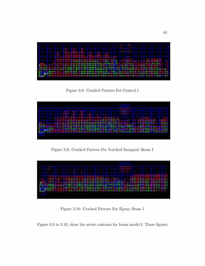
61
Figure 3.8: Cracked Pattern For Control I
Figure 3.9: Cracked Pattern For Notched Inorganic Beam I
Figure 3.10: Cracked Pattern For Epoxy Beam I
Figure 3.8 to 3.10, show the stress contours for beam model I. Those figures
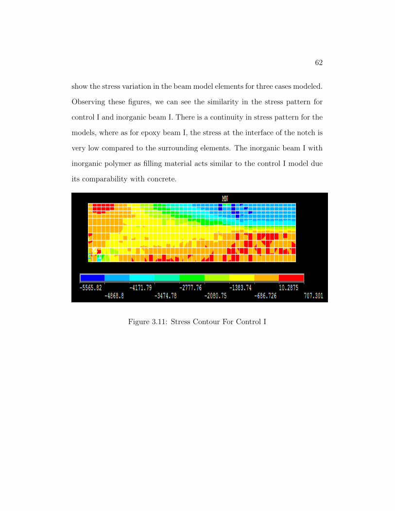
62
show the stress variation in the beam model elements for three cases modeled.
Observing these figures, we can see the similarity in the stress pattern for
control I and inorganic beam I. There is a continuity in stress pattern for the
models, where as for epoxy beam I, the stress at the interface of the notch is
very low compared to the surrounding elements. The inorganic beam I with
inorganic polymer as filling material acts similar to the control I model due
its comparability with concrete.
Figure 3.11: Stress Contour For Control I

63
Figure 3.12: Stress Contour For Inorganic Beam I
Figure 3.13: Stress Contour For Epoxy Beam I
Figure 3.11 shows a graph plotted for the elastic strain of elements at a
location near the mid span of the quarter beam. The figure shows the elastic
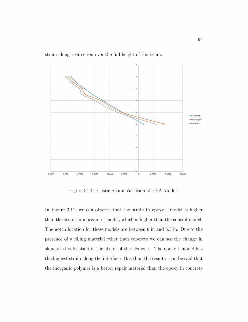
64
strain along x direction over the full height of the beam.
Figure 3.14: Elastic Strain Variation of FEA Models
In Figure 3.11, we can observe that the strain in epoxy I model is higher
than the strain in inorganic I model, which is higher than the control model.
The notch location for these models are between 6 in and 6.5 in. Due to the
presence of a filling material other than concrete we can see the change in
slope at this location in the strain of the elements. The epoxy I model has
the highest strain along the interface. Based on the result it can be said that
the inorganic polymer is a better repair material than the epoxy in concrete
65
applications.
Figure 3.12 shows the load displacement plot for the three cases. The dis-
placement at the right end of the quarter beam was recorded for a node
using the time history post processor tool in ANSYS. The displacement of
the node at various load sub steps is stored. Similarly the force applied on
the structure at various sub steps is plotted in Figure 3.12. Figure shows
the force on y axis and the displacement on the x axis for the three cases
modeled for beam model I.

66
Figure 3.15: Load Displacement Plot
Looking at the load displacement plot, we can notice that the response of the
structure to the load filled with repair material is very close to that of the
original structure. The stiffness of the beam repaired with epoxy is slightly
lower than the beam repaired with inorganic polymer. The effect of thickness
of the adhesive interface on the response of the structure can be seen in the
load deformation plot of beam model II, shown in Figure 3.17.
67
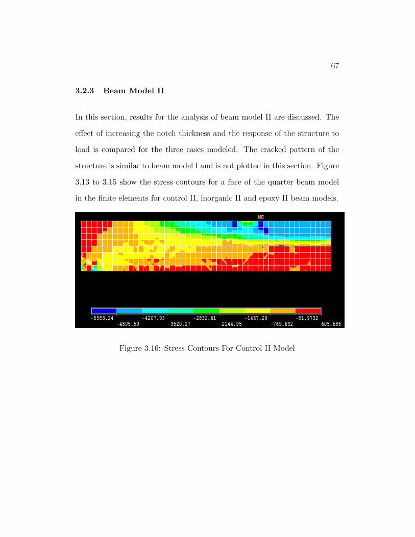
3.2.3 Beam Model II
In this section, results for the analysis of beam model II are discussed. The
effect of increasing the notch thickness and the response of the structure to
load is compared for the three cases modeled. The cracked pattern of the
structure is similar to beam model I and is not plotted in this section. Figure
3.13 to 3.15 show the stress contours for a face of the quarter beam model
in the finite elements for control II, inorganic II and epoxy II beam models.
Figure 3.16: Stress Contours For Control II Model
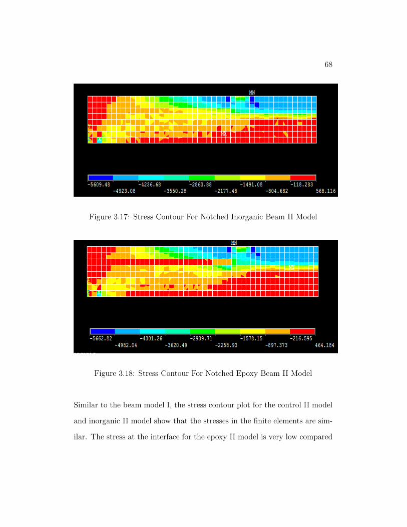
68
Figure 3.17: Stress Contour For Notched Inorganic Beam II Model
Figure 3.18: Stress Contour For Notched Epoxy Beam II Model
Similar to the beam model I, the stress contour plot for the control II model
and inorganic II model show that the stresses in the finite elements are sim-
ilar. The stress at the interface for the epoxy II model is very low compared
69
to its boundary elements. It can be said that repairing the concrete beam
with inorganic polymer would make the beam almost behave like the original
undamaged structure.
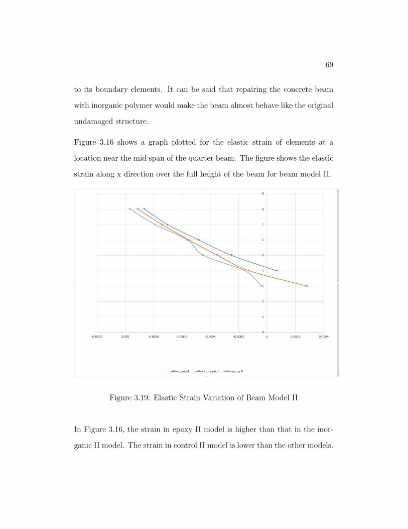
Figure 3.16 shows a graph plotted for the elastic strain of elements at a
location near the mid span of the quarter beam. The figure shows the elastic
strain along x direction over the full height of the beam for beam model II.
Figure 3.19: Elastic Strain Variation of Beam Model II
In Figure 3.16, the strain in epoxy II model is higher than that in the inor-
ganic II model. The strain in control II model is lower than the other models.
70
The notch location to be repaired in the model is 1 inch thick located be-
tween 5 and 6 inch depth of the beam. Looking at the graph we can see the
similarity in the behavior of the beam filled with inorganic polymer and the
control II beam. The strain variation along the height of the cross section
is uniform for both models . In the epoxy beam model II, the variation of
the elastic strain is not uniform at the notch location, as we can see with
the change in slope of the curve between point 5 and 6 along the y axis. It
can be said that the beam repaired with inorganic polymer responds to the
load applied on the structure similar to the control beam, whereas a beam
repaired with epoxy might not be as compatible with concrete as the beam
repaired with inorganic polymer. Comparing Figures 3.16 and 3.11, we can
see the effect of thickness of the on the variation of strain along the height
of the beam. It seems the thicker inorganic adhesive repair has a uniform
transition at the notch location.
The graph shown in Figure 3.17 show the load displacement plot for beam
model II when loaded till failure for the three cases modeled. The displace-
ment at the end of the quarter beam was recorded using the time history
post processing tool in ANSYS. Similarly the force applied on the structure
is recorded for the various load steps and is plotted on the y axis, whereas
the displacement is plotted on the x axis to the corresponding load step.
71
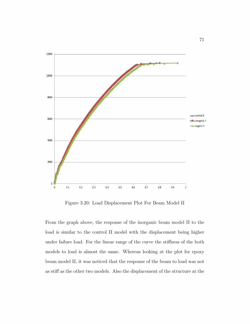
Figure 3.20: Load Displacement Plot For Beam Model II
From the graph above, the response of the inorganic beam model II to the
load is similar to the control II model with the displacement being higher
under failure load. For the linear range of the curve the stiffness of the both
models to load is almost the same. Whereas looking at the plot for epoxy
beam model II, it was noticed that the response of the beam to load was not
as stiff as the other two models. Also the displacement of the structure at the

72
failure load is much higher in comparison. Comparing the load displacement
plot for beam model I and beam model II, the increased thickness has a
pronounced effect on the response of the structure to the load. A further
study is conducted on the effect of varying the elastic modulus of the organic
epoxy system and is reported in the appendix.
3.2.4 Slab Model
In this section, the results for the analysis of the slab model are discussed.
Four FE models were developed to study the response of the slab to the
applied loads. These models are 1) control case,2) slab repaired with epoxy
,3) slab repaired with inorganic polymer and 4)fourth situation where slab is
delaminated but does not have any repair material. The fourth case is mod-
eled with elements having the properties of air at the interface for the sake of
continuity and to simulate the behavior of the delmaninated structure. The
load displacement response is shown in Figure 3.18 to compare the various
FE models. The models have three delaminated zones. These zones were
used to study the response of the structure for multiple repair zones in a slab
which is common practice in field application.
73
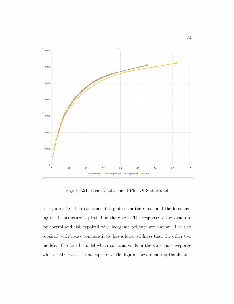
Figure 3.21: Load Displacement Plot Of Slab Model
In Figure 3.18, the displacement is plotted on the x axis and the force act-
ing on the structure is plotted on the y axis. The response of the structure
for control and slab repaired with inorganic polymer are similar. The slab
repaired with epoxy comparatively has a lower stiffness than the other two
models. The fourth model which contains voids in the slab has a response
which is the least stiff as expected. The figure shows repairing the delami-

74
nated slab with epoxy or inorganic polymer is more effective and can behave
in a similar way to the original structure and exhibiting similar original stiff-
ness.

75
4 Conclusions and Recommendations
In the previous sections, a detail description of the model and the results
obtained in this research along with a discussion were provided. Based on
the results obtained in the analytical investigation the following conclusions
can be drawn:
•The results of finite element based method adopted to analyze the load
deformation response of repaired beams compared reasonably well with the
experimental results. The finite element approach showed a slightly stiffer
response than the experimental investigation. The selections of elements to
model concrete, steel rebar , epoxy and inorganic polymer was validated in
this model. The material laws attributed to the elements was also ascer-
tained.
•The bond slip interaction at the steel concrete interface was included in
the model and was accounted for by incorporating the bond slip relation
at the interface using zero length spring elements. The results of the FE
model showed similar response to the experimental results. The bond slip
interaction of the steel concrete interface should be considered because of
presence of micro cracks due to shrinking or cracks developed during the
placement of concrete and other conditions of the interface.
•The stress at the interface or the notch location was compared for the two
beam models I and II. In both models it was observed that the beam re-
76
paired with inorganic polymer behaved similar to the control beam, whereas
the stress in epoxy material at the interface is very low compared to its
surrounding elements. This seems to indicate that the inorganic polymer is
more compatible with the surrounding concrete elements.
•In the two beams modeled, the beam with a 1 inch thick filler material
showed considerable difference in the elastic strain along the longitudinal
direction for the various filler materials. The inorganic polymer repaired
beam had a higher strain but maintained the same slope throughout its
height, whereas the beam repaired with epoxy had the highest strain and
also there strain variation along the height of the beam was not uniform. The
results showed that the inorganic polymer is more compatible with concrete
than epoxy.
•The load deformation response for both the beam models with the various
filler materials showed that the inorganic polymer behavior is similar to con-
crete, whereas the response of the beam repaired with epoxy was less stiff
compared to concrete. This difference in response increased with the increase
in thickness of the filler material.
•The load deformation response of the four FE slab models developed in
this investigation showed the slab modeled with inorganic filler material was
similar to the original slab.

77
Recommendations :
•Further investigation of the nature of the bond slip characteristics between
the inorganic polymer and the concrete is needed. Also the nature of bond
slip characteristics between epoxy and concrete needs further investigation
in finite element analysis studies.
•Its common to have some inaccuracies in the structure and when loaded the
defects on the tension side could increase with the tensile cracking of concrete.
A study should be conducted to investigate the effects of crack propagation
with a fracture mechanics based approach in ANSYS using either the VCCT
approach or using cohesive zone modeling. The effect of these defects on the
stiffness and capacity beams and slabs is worth further investigation.
•The elements selected in this study can be used for further applications
related to finite element modeling of reinforced concrete structures. The
zero length spring element used in this study to model the bond slip relation
at the steel concrete interface can be used for the study of bond slip relation
for two way slabs where the effect could be more pronounced.
•The inorganic polymer investigated in this study could be used as an adhe-
sive to bond FRP to concrete structures on the tension side of the surface.
A FE based approach could be adopted to investigate the response of the
structure with layered solid elements for FRP, soild65 elements for concrete
and adhesive, link180 elements for steel rebar. Also a bond slip interaction
model could be incorporated for the slip at the interface.

78
References
[1] Foden, Andrew J. 1999.Mechanical Properties and Material Characteriza-
tion of Polysialate Structural Composites. Dissertation. New Brunswick,
NJ: Rutgers, The State University of New Jersey, January.
[2] Iowa DOT, Office of Materials. 1998. Inspection and Acceptance of Epoxy
Injection Resins. Ames: Iowa Department of Transportation.
[3] Krauss, Paul D., John M. Scanlon, Margaret A. Hanson, and Wiss, Janney,
Elstner Associates, Inc. 1995. Evaluation of Injection Materials for the Re-
pair of Deep Cracks in Concrete Structures. Washington, D.C.: US Army
Corps of Engineers
[4] Klein,Matthew.2013.Destructive repair and Rehabilitation Of Struc-
tural Elements Using High Strength Inorganic Polymer Compos-
ites.Dissertation.New Brunswick,NJ:Rutgers,The State University of New
Jersey.
[5] Stratton, F. Wayne, Roger Alexander, and William Nolting. 1978.Cracked
Structural Concrete Repair Through Epoxy Injection and Rebar Inser-
tion.Final, Topeka: Kansas Department of Transportation.
[6] Stratton, F. Wayne, and Barbara J. Smith. 1988.Bridge Deck Hollow Plane
Repair Using Injected Epoxy. Topeka: Kansas Department of Transporta-
tion.
[7] SealBoss. 2012. Sealboss 4040 LV Epoxy Resin. Product Data Sheet, Santa
Ana: SealBoss Corporation.
79
[8] Kachlakev,Damian.Miller,Thomas.Finite Element Modeling Of Concrete
Structures Strengthened With FRP laminates.Oregon department of trans-
portation.
[9] William,K.J and E.P.Warnked,”Constitutive Model for the triaxial Behavior
of Concrete”,Proceedings,International Association for Bridge and Struc-
tural Engineering,Vol 19,ISMES,Bergamo,Italy,pp.174,1975.
[10] Desayi,p.and S.krishnan,”Equation for the Stress-Strain curve of Con-
crete”,Journal of the American Concrete Institute,61,pp.345-350,March
1964.
[11] Wolanski,Anthony.J(2004).Flexural Behavior of Reinforced and Prestressed
Concrete Beams Using Finite Element Analysis. Master’s thesis, Milwau-
kee,Wisconsin.
[12] Tavarez,F,A.,(2001)”Simulation of Behavior of Composite Grid Reinforced
Concrete Beams Using Explicit Finite Element Methods”,Master’s the-
sis,University if Wisconsin-Madison,Wisconsin.
[13] Yang Xiaoming,Zhu Hongqiang.”Finite Element Investigation on Load Car-
rying Capacity of corroded RC Beam Based on Bond-slip”.Jordan Journal
of Civil Engineering,Volume 6,No.1,2102.
[14] Job Thomas,Ananth Ramaswamy.(2006).”Nonlinear Analysis of Shear
Dominant Prestressed Concrete Beams using ANSYS”.
[15] ANSYS V14.5,Mechanical Users Guide, Modeling and Meshing Guide.
[16] concreteanswers.org.
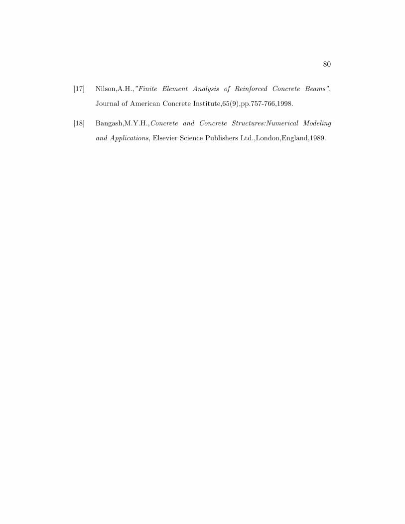
80
[17] Nilson,A.H.,”Finite Element Analysis of Reinforced Concrete Beams”,
Journal of American Concrete Institute,65(9),pp.757-766,1998.
[18] Bangash,M.Y.H.,Concrete and Concrete Structures:Numerical Modeling
and Applications, Elsevier Science Publishers Ltd.,London,England,1989.
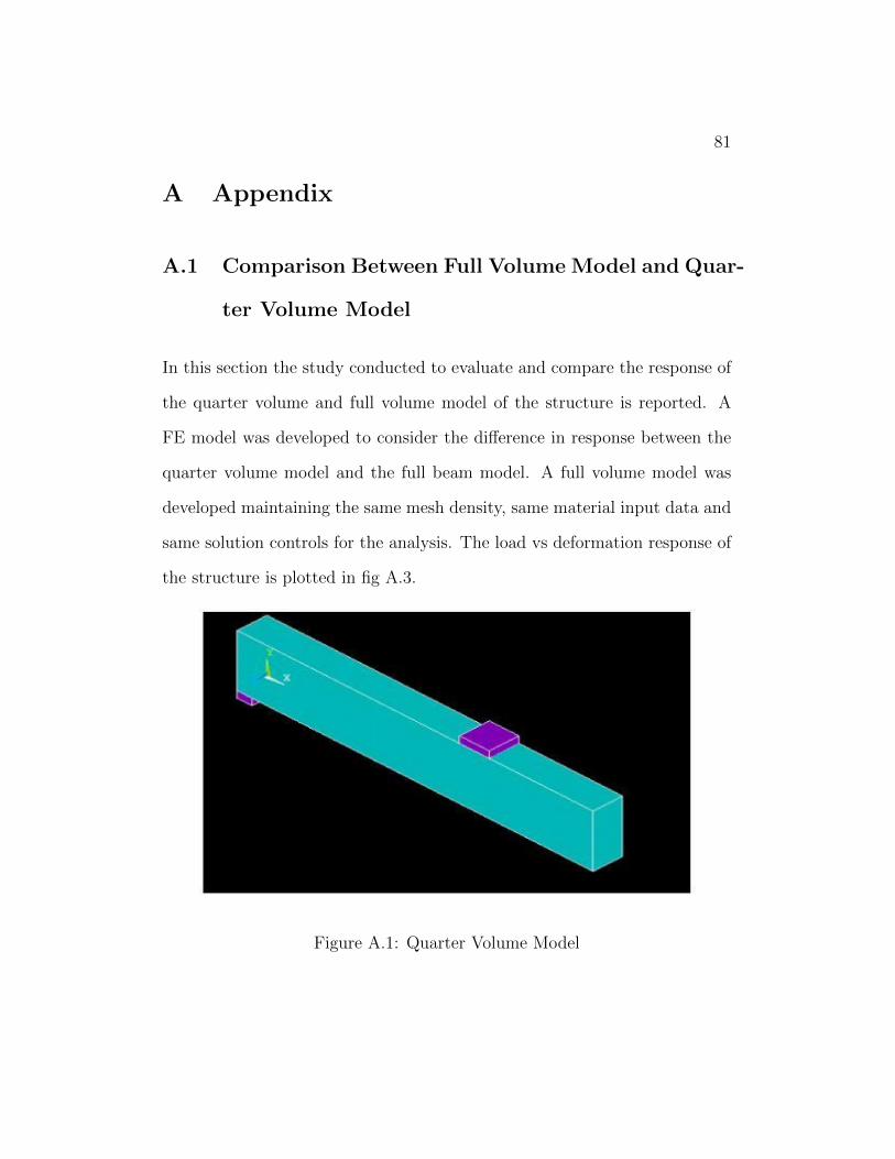
81
A Appendix
A.1 Comparison Between Full Volume Model and Quar-
ter Volume Model
In this section the study conducted to evaluate and compare the response of
the quarter volume and full volume model of the structure is reported. A
FE model was developed to consider the difference in response between the
quarter volume model and the full beam model. A full volume model was
developed maintaining the same mesh density, same material input data and
same solution controls for the analysis. The load vs deformation response of
the structure is plotted in fig A.3.
Figure A.1: Quarter Volume Model

82
Figure A.2: Full Volume Model
Figure A.3: Load Deformation Response from Quarter and Full Beams Mod-
els
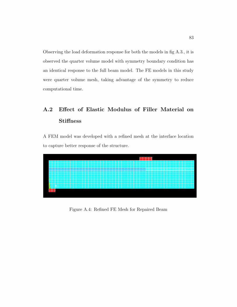
83
Observing the load deformation response for both the models in fig A.3., it is
observed the quarter volume model with symmetry boundary condition has
an identical response to the full beam model. The FE models in this study
were quarter volume mesh, taking advantage of the symmetry to reduce
computational time.
A.2 Effect of Elastic Modulus of Filler Material on
Stiffness
A FEM model was developed with a refined mesh at the interface location
to capture better response of the structure.
Figure A.4: Refined FE Mesh for Repaired Beam
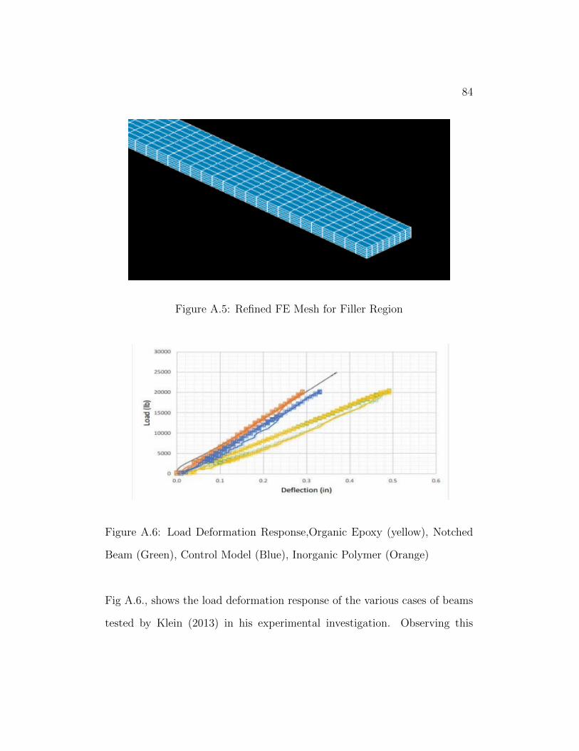
84
Figure A.5: Refined FE Mesh for Filler Region
Figure A.6: Load Deformation Response,Organic Epoxy (yellow), Notched
Beam (Green), Control Model (Blue), Inorganic Polymer (Orange)
Fig A.6., shows the load deformation response of the various cases of beams
tested by Klein (2013) in his experimental investigation. Observing this
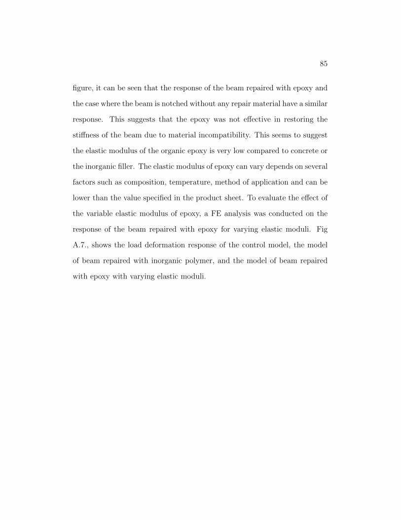
85
figure, it can be seen that the response of the beam repaired with epoxy and
the case where the beam is notched without any repair material have a similar
response. This suggests that the epoxy was not effective in restoring the
stiffness of the beam due to material incompatibility. This seems to suggest
the elastic modulus of the organic epoxy is very low compared to concrete or
the inorganic filler. The elastic modulus of epoxy can vary depends on several
factors such as composition, temperature, method of application and can be
lower than the value specified in the product sheet. To evaluate the effect of
the variable elastic modulus of epoxy, a FE analysis was conducted on the
response of the beam repaired with epoxy for varying elastic moduli. Fig
A.7., shows the load deformation response of the control model, the model
of beam repaired with inorganic polymer, and the model of beam repaired
with epoxy with varying elastic moduli.
86
Figure A.7: Load Deformation Response from FE Models for Various Cases
Observing the load deformation response in fig A.7., it is observed that the
load deformation response of the beam repaired with organic epoxy with an
elastic modulus of 0.18E+05 psi has the least stiffness as expected. The
figure also shows considerable difference in stiffness compared to the beam
repaired with organic epoxy but with higher modulus.
87
A.3 Effect of Shear Retention
The tensile cracking which occurs in concrete is generally modeled in FEA
by two approaches. In the first approach which is known as discrete element
method, the cracks developed in the concrete are locally modeled in this
approach. Separation between adjacent elements representing the crack has
to be accurately modeled. The limitation of this method is that one needs
to know the cracking path prior to performing FE analysis. Initial meshing
should comply with this path and also the FE mesh needs to be regenerated
at every crack-propagation step. This makes this analysis time-consuming
and expensive.
The alternative method assumes a smeared crack approach which considers
fracture distribution over damaged region. So, this geometrical nonlinearity
may be simulated with material stiffness degradation while crack propagation
occurs. This option of concrete modeling can be selected by modeling the
structure with SOLID65 element available in ANSYS. SOLID65 is modeled as
a 3D solid with 8 nodes. This element is a linear order element, which might
be overly stiff in bending dominated problems. Higher order displacement
response cannot be assigned to this element, this is one of the limitation of
the SOLID65 element.
Shear transfer coefficient which needs to be input for the concrete model
varies from 0.0 to 1.0, with 0.0 representing a smooth crack (complete loss of
shear transfer) and 1.0 representing a rough crack (no loss of shear transfer).
88
This specification may be made for both the closed and open crack. A shear
transfer coefficient of 0.3 was adopted in the study, choosing an appropriate
factor for shear transfer coefficient is very important. Improper selection of
the factor might lead to shear locking leading to stiffer elements.
To evaluate the effect of the shear retention factor on the load deformation
response, several FE models were developed for variable values of the shear
retention factors. Fig A.8., shows the load deformation response of the FE
models with varying shear retention factor for open crack. These FE plots are
compared to the experimental load deformation response from Klein (2013).
The assumptions made in FE models were the following:
•Concrete is cracked before the load was applied (tensile strength 10 psi).
•Inorganic polymer was given a tensile strength of 530 psi (not cracked ini-
tially).
•Elastic modulus of organic epoxy was taken as 1E+05 psi.
•A higher displacement convergence criteria of 0.025 compared to 0.005 was
given for concrete with shear coefficient 0.01 for the sake convergence. (dis-
placement convergence criteria = Ui+1 − Ui < Value Specified)

89
Figure A.8: Load Deformation Response for the Concrete Model
Observing the load deformation response for the various cases, it is seen that
concrete with a shear retention factor of 0.3 was the stiffest and had the
highest failure load with the steel yielding before compression failure. The
model with a shear retention value of 0.1 was least stiff and was comparable
to the response of the experimental beam but failed at a much lower load
compared to the beam with a shear coefficient of 0.3.
The load deformation response for the beams repaired with inorganic polymer
and with organic epoxy with a shear coefficient of 0.1 and 0.3 for open crack
in concrete is also plotted in figures A.9., and A.10., respectively. The load
deformation response of the repaired beams also show that the beam is stiffer

90
when the shear retention factor is higher.
Figure A.9: Load Deformation Response for Beam Repaired with Inorganic
Polymer for Various Shear retention 0.1 and 0.3

91
Figure A.10: Load Deformation Response for Beam Repaired with Organic
Epoxy for Various Shear retention 0.1 and 0.3
Conclusion
The FE study of reinforced concrete is complex due to the nature of the
material. In finite element modeling of reinforced concrete beams, there are
various factors that affect load deformation response of the beam such as the
shear retention factor, the mesh density, the bond-slip interaction at the steel
concrete interface and also the approach to crack modeling due to cracking
92
in tension. Employing Newton-Raphson method for non-linear analysis also
has its limitation as concrete has to be modeled as perfectly plastic after
reaching its maximum stress. General FE purpose programs such as ANSYS
may be used to evaluate the response of reinforced concrete beams but has
its limitations.