Graduate Theses, Dissertations, and Problem Reports

2013

Analytical and Computational Study of Flame Acceleration in Analytical and Computational Study of Flame Acceleration in

Tubes: Effect of Wall Friction Tubes: Effect of Wall Friction

Berk Demirgok West Virginia University

Follow this and additional works at: https://researchrepository.wvu.edu/etd

Recommended Citation Recommended Citation Demirgok, Berk, "Analytical and Computational Study of Flame Acceleration in Tubes: Effect of Wall Friction" (2013). Graduate Theses, Dissertations, and Problem Reports. 301. https://researchrepository.wvu.edu/etd/301

This Thesis is protected by copyright and/or related rights. It has been brought to you by the The Research Repository @ WVU with permission from the rights-holder(s). You are free to use this Thesis in any way that is permitted by the copyright and related rights legislation that applies to your use. For other uses you must obtain permission from the rights-holder(s) directly, unless additional rights are indicated by a Creative Commons license in the record and/ or on the work itself. This Thesis has been accepted for inclusion in WVU Graduate Theses, Dissertations, and Problem Reports collection by an authorized administrator of The Research Repository @ WVU. For more information, please contact researchrepository@mail.wvu.edu.

Analytical and Computational Study of Flame Acceleration in Tubes:

Effect of Wall Friction

Berk Demirgok

Thesis submitted to the

Benjamin M. Statler College of Engineering and Mineral Resources

at

West Virginia University

in Partial Fulfillment of the Requirements for the Degree of

Master of Science

in

Mechanical Engineering

V’yacheslav Akkerman, Ph.D., Chair

Ismail B. Celik, Ph.D.

Halin Li, Ph.D.

Scott W. Wayne, Ph.D.

Department of Mechanical and Aerospace Engineering

Morgantown, West Virginia

(2013)

Keywords: combustion, theory, modeling, flame acceleration, tubes, channels

Copyright 2013 Berk Demirgok

ii

ABSTRACT

Analytical and Computational Study of Flame Acceleration in Tubes:

Effect of Wall Friction

Berk Demirgok

Premixed flame acceleration is especially strong in the case of flame propagation in tubes or

channels. Being a reasonably simple configuration to investigate fundamental flame

properties, combustion tubes have numerous practical applications such as safety issues in

mines, subways and power plants. This work is devoted to the analytical formulation and

computational simulations of premixed flame acceleration induced by wall friction in

tubes/channels. Specifically, the evolution of the flame dynamics and morphology is

determined, and the main characteristics of the flame acceleration such as the flame shape and

propagation speed, the acceleration rate as well as the combustion-generated velocity profile

in the fresh premixture are quantified. It is shown that the flame acceleration is promoted with

the increase in the thermal expansion in the burning process, whereas it weakens with the

increase in the Reynolds number. The intrinsic accuracy and the limitations of the analytical

theory are determined and validated by means of direct numerical simulations. Computational

and analytical results are compared with recent experiments, and the numerical simulations

bridge a certain gap between the experimental measurements and analytical formulations.

iii

Acknowledgements

I would like to express my gratitude to several key persons who have contributed towards the

completion of this thesis and have influenced my professional development as a researcher.

First and foremost, I would like to thank Dr. V’yacheslav Akkerman, who initially gave me

the opportunity to pursue my educational career with WVU, and continuously provided me

with his huge support and guidance throughout my time here. I sincerely thank my

committee members, Dr. Ismail B. Celik, Dr. Hailin Li and Dr. Scott W. Wayne for their

valuable time and suggestions. I am also very grateful to my friends and lab partners for

useful discussions.

Also, I would like to acknowledge Dr. Damir Valiev of Sandia National Laboratories,

Livermore, CA. The computational component of this thesis would not be possible without

his comprehensive support and consulting.

Besides, I am thankful to Dr. Ming-Hsun Wu of Taiwan National Cheng Kung University,

who provided us with his experimental data.

Finally, I would like to mention my family that never questioned my ability of obtaining an

advanced degree and that has stuck by my side throughout.

iv

I dedicate this thesis to my parents Bulent Demirgok and Zahide Demirgok.

v

Table of Contents

Abstract… … … … … … … … … … … … ii

Acknowledgments… … … … … … … … … … … iii

Dedication… … … … … … … … … … … … iv

Table of Contents… … … … … … … … … … … v

Nomenclature… … … … … … … … … … … vii

List of Figures… … … … … … … … … … … xi

Chapter 1: Introduction... … … … … … … … … 1

1.1. Fundamentals of Combustion… … … … … … … … 1

1.2. Overview and Objectives… … … … … … … … 5

1.2.1. Overview... … … … … … … … … … 5

1.2.2. Objectives… … … … … … … … … … 9

Chapter 2: Theory of Flame Acceleration in Tubes due to Wall Friction:

Intrinsic Limitations and Accuracy… … … … … … … 10

2.1. Basics of the Bychkov-Akkerman Formulation… … … … … … 10

2.2. Flame Acceleration in a 2D Channel… … … … … … … 13

2.3. Flame Acceleration in a Cylindrical Tube … … … … … … 20

2.4. Conclusions… … … … … … … … … … 28

Chapter 3: Computational Platform … … … … … … … 29

3.1. Governing Equations… … … … … … … … … 29

3.2. Numerical Scheme… … … … … … … … … 34

3.3. Principal of Setting of the Initials Conditions… … … … … … 36

vi

Chapter 4: Effect of Thermal Expansion on Flame Propagation in Channels

with Nonslip Walls: Numerical and Analytical Consideration... … … 38

4.1. Motivation… … … … … … … … … … 38

4.2. Computational Results and Discussion… … … … … … … 39

4.3. Conclusions… … … … … … … … … … 52

Chapter 5: Analysis of Ethylene-Oxygen Combustion in Micro-Pipes… … 53

5.1. Formulation… … … … … … … … … … 53

5.2. Experiments… … … … … … … … … … 55

5.3. Computational Simulations… … … … … … … … 56

5.4. Results and Discussion… … … … … … … … … 57

5.5. Conclusions… … … … … … … … … … 61

Chapter 6: Summary … … … … … … … … … 62

References… … … … … … … … … … … … 63

APPENDIX A… … … … … … … … … … … 65

APPENDIX B… … … … … … … … … … … 75

APPENDIX C… … … … … … … … … … … 76

vii

Nomenclature

Letters

A Reaction rate

Cp [J/Kg] Heat capacity

CPU Central processing unit

DL Darieus- Landau

DNS Direct numerical simulations

Dth [m2/s] Thermal diffusivity

Ea [kj/mol] Activation energy

Lf [m] Flame front thickness

Ma Mach number

mb [g/mol] molecular weight of the burnt matter

mf [g/mol] molecular weight of the fuel mixture

n normal vector

P [Pa] Pressure

Pr Prandtl number

Q [J] Energy release from the reaction

qi energy diffusion vector component

R [mm] Radius of a tube

RAM Random memory access

Re Reynolds number

Rp [J/molK] Universal gas constant

S2D [m] Total length of the flame front in a 2D

viii

geometry

Scyl [m] Total length of the flame front in an axisymmetric geometry

Sc Schmidt number

Sf [m2] The area of the plane front

Sw [m2] Surface area of the curved flame

T [K] Temperature

Tb [K] Temperature of the burnt matter

Uf [cm/s] Unstretched laminar (planar) flame speed

Utip [cm/s] Flame tip velocity

Uw [cm/s] Curved flame velocity

uz Flow velocity related to burning rate

WVU West Virginia University

Greek Symbols

Ωw Scaled flame velocity

σ Dimensionless acceleration rate

σnumerical Dimensionless acceleration rate of the numerical approach

σanalytical Dimensionless acceleration rate of the analytical approach σ0 Dimensionless acceleration rate in the 0th order approximation σ1 Dimensionless acceleration rate in

ix

the 1st order approximation ζij Stress tensor

τ Scaled time

τR Characteristic time

ν [kg/s.m] Kinematic viscosity

μ [kg/s.m] Dynamic viscosity

ξtip Scaled flame tip position

ρb [kg/m3] Density of the burnt matter

ρf [kg/m3] Density of the fuel

π Pi number

Ωss Parameter characterizing the total burning rate in the isobaric limit

Θ Thermal expansion coefficient

κ Thermal conduction coefficient

x

List of Figures

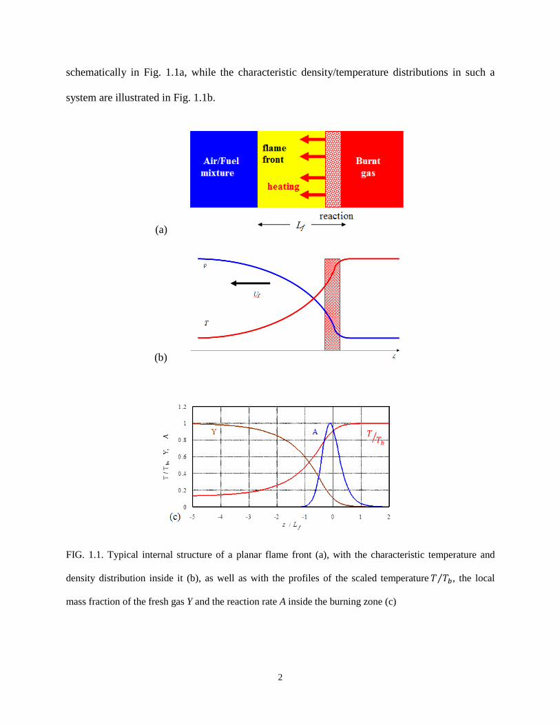
FIG. 1.1. Typical internal structure of a planar flame front (a), with the characteristic temperature

and density distribution inside it (b), as well as with the profiles of the scaled temperature 𝑇 𝑇𝑏⁄ , the

local mass fraction of the fresh gas Y and the reaction rate A inside the burning zone (c) … 2

FIG. 1.2. Evolution of a finger flame front… … … … … … … … 7

FIG. 1.3 Wall friction (Shelkin) scenario of flame acceleration in smooth tubes… … … 7

FIG. 1.4. Schematic of the physical mechanism of flame acceleration in obstructed tube … 8

FIG. 2.1. A flame in a tube or channel with non-slip at the walls… … … … … 11

FIG. 2.2. The flame acceleration rate σ versus the flame propagation Reynolds number Re at the

fixed thermal expansion coefficients 10;8;6;4=Θ . Equations (2.8) and (2.10) are shown by

dashed and solid lines, respectively… … … … … … … … 16

FIG. 2.3. The flame acceleration rate σ versus the thermal expansion coefficient Θ at the fixed

flame propagation Reynolds numbers Re = 5; 10; 20. Equations (2.8) and (2.10) are shown by

dashed and solid lines, respectively… … … … … … … … 17

FIG. 2.4. Relative error (in %) versus thermal expansion coefficient Θ at fixed propagation

Reynolds numbers such as Re = 20, 10 and 5 shown by dotted, dashed and solid lines, respectively

(a); and the relative error percentage versus propagation Reynolds number at fixed thermal

expansion such as Θ =10, 8, 6 and 4 shown by solid &dotted, dashed, dotted and solid lines,

respectively (b)… … … … … … … … … … … 19

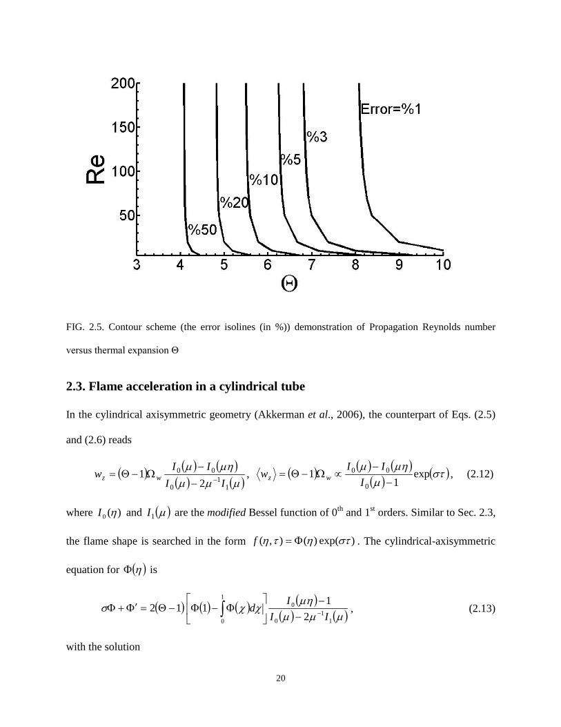
FIG. 2.5. Contour scheme (the error isolines (in %)) demonstration of Propagation Reynolds

number versus thermal expansion Θ… … … … … … … … 20

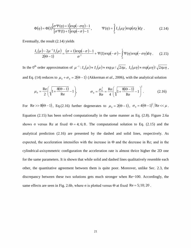
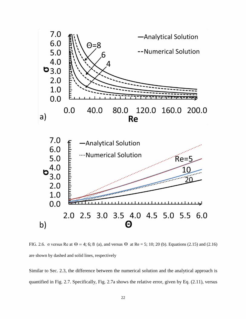
FIG. 2.6. σ versus Re at 8;6;4=Θ (a), and versus Θ at Re = 5; 10; 20 (b). Equations (2.15) and

(2.16) are shown by dashed and solid lines, respectively… … … ... … … 22

FIG. 2.7. The relative error (in %), Eq. (2.11), versus Θ at Re = 5, 10, 20, shown by solid, dashed

and dotted lines, respectively (a); and versus Re at Θ = 3, 4, 6 shown by solid, dashed and dotted

lines, respectively (b)… … … … … … … … … … 23

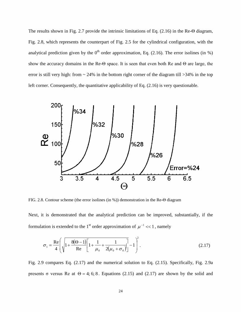
FIG. 2.8. Contour scheme (the error isolines (in %)) demonstration in the Re-Θ diagram … 24

FIG. 2.9. σ versus Re at 8;6;4=Θ (a); and versus Θ at Re = 5; 10; 20 (b). Equations (2.15) and (2.17) are

shown by dashed and solid lines, respectively … … … … … … … 25

xi

FIG. 2.10. The relative error (in %), Eq. (2.11), versus Θ at Re = 5, 10, 20, shown by solid, dashed

and dotted lines, respectively (a); and versus Re at Θ = 3, 4, 6 shown by solid, dashed and dotted

lines, respectively (b) … … … … … … … … … … 27

FIG. 2.11. Contour scheme (the error isolines (in %)) demonstration in the Re-Θ diagram … 28

FIG. 3.1. The sketch of the grid with variable resolution used in numerical simulations … … 32

FIG. 3.2. Profiles of the scaled temperature T/Tb, the mass fraction Y, and the reaction rate… ….

A ∝ (ρY/τr)× exp(−Ea/RpTb), scaled by its maximal value… … … … … 34

FIG. 4.1. The scaled flame tip position ξtip versus the scaled time τ at fixed thermal expansion coefficients,

namely Θ = 12 (a), Θ = 10 (b), Θ = 9 (c), and Θ = 8 (d), with various flame propagation Reynolds numbers

in each plot and the scaled flame tip position ξtip versus the scaled time τ at thermal expansion coefficients Θ

= 12, 10, 8 and 6 and fixed propagation Reynolds number Re = 20 (e) Re = 10 (f)… … … 43

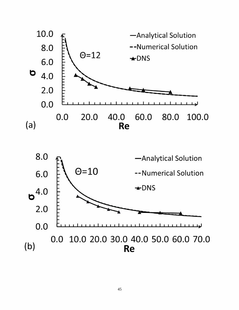
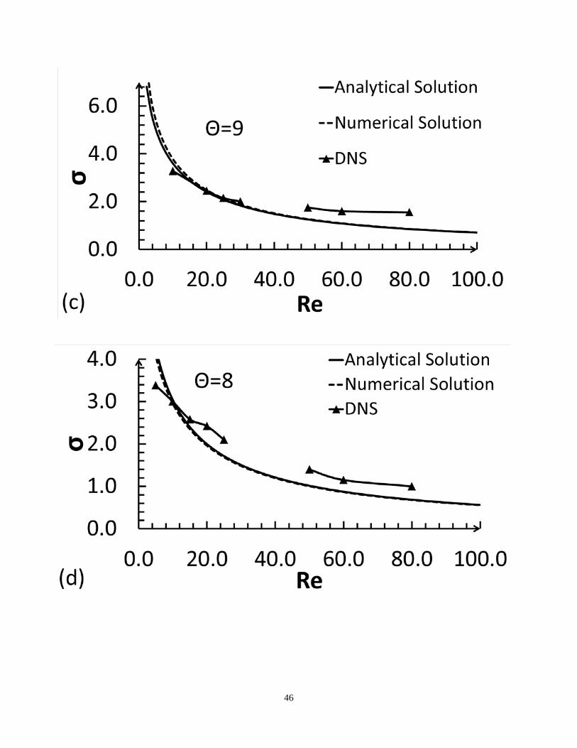
FIG. 4.2. The flame acceleration rate σ versus propagation Reynolds number Re at thermal expansion Θ = 12

(a), 10 (b), 9 (c), 8 (d), 7 (e), 6 (f)... … ... … … … … … … … … … 47

FIG. 4.3. The scaled flame tip position ξtip versus the scaled time τ at fixed thermal expansion coefficient Θ =

5 and flame propagation Reynolds numbers Re = 30 (a). The scaled flame tip velocity Utip /Uf versus the

scaled time τ at fixed thermal expansion coefficient Θ = 5 and flame propagation Reynolds numbers Re = 30

(b). The scaled flame tip position ξtip versus the scaled time τ at fixed thermal expansion coefficient Θ = 4

and flame propagation Reynolds numbers Re = 40 (c). The scaled flame tip velocity Utip /Uf versus the scaled

time τ at fixed thermal expansion coefficient Θ = 4 and flame propagation Reynolds numbers Re = 40 (d)

… … … … … … … … … … … … … … … … … … … 50

FIG. 4.4. Evolution of the flame shape for a small thermal expansion, 4=Θ Fig. 4.3 (a-c) as well as for the

realistically large one, 9=Θ Fig. 4.3 (d-f)… … … … … … … … 51

FIG. 5.1. Evolution of the flame tip in a tube of radii R=0.25 mm (a) and 0.5mm (b)… … … 58

FIG. 5.2. Evolution of the flame tip in a tube of R = 0.25 mm for Ωss = 4.2. The cases of the

acceleration rate given by Eq. (2.17), 1σ and Eq. (2.16), 0σ , are shown by the dashed and solid

lines, respectively. Filled rectangles show the experimental results while dotted line represents the

DNS ones… … … … … … … … … … … … … 59

FIG. 5.3. Evolution of the flame tip in a tube of R = 0.5 mm for Ωss = 4.2. The cases of the

acceleration rate given by Eq. (2.17), ,1σ and Eq. (2.16), 0σ , are shown by the dashed and solid

xii

lines, respectively. Filled rectangles show the experimental results while dotted line represents the

DNS ones… … … … … … … … … … … … … 59

FIG. 5.4. Evolution of the flame tip in a tube of R = 0.5 mm for Ωss = 7.1. The cases of the acceleration rate

given by Eq. (2.16), 1σ , and Eq. (5.16), 0σ , are shown by the dashed and solid lines, respectively. Filled

rectangles show the experimental results while dotted line represents the DNS ones … … … 60

FIG. 5.5: Evolution of the flame shape in a tube of radius R = 56Lf = 0.25mm. The colors represent the

temperature from 300K in the fuel mixture (blue) to the corresponding burnt matter temperature (red)… 61

1

Chapter 1: Introduction

1.1. Fundamentals of Combustion

What is Combustion? While it can generally be defined as an exothermal chemical reaction, such

a definition incorporates a great variety of different processes, starting with standard oxidation of

coal, oil, natural gas, alcohol and hydro-carbon fuels, and ending with astrophysical applications

like thermonuclear reactions in Supernovae. This thesis is limited to burning of premixed air-fuel

mixture, when all chemical components, necessary for the reaction, are present in a air-fuel

mixture from the very beginning. In that case, if the heat release in the burning process exceeds

the thermal losses, then the reaction is self-supporting, and once ignited, the reaction typically

spreads through the gas as a rather thin, well-localized front until all the fuel is burned. Such a

scenario is typically observed in car engines, subways, mines or various laboratory setups.

Basically, two main self-supporting regimes of combustion are distinguished: a flame (also

known as deflagration) and a detonation (Bychkov and Liberman, 2000). In the case of a flame,

the reaction propagates due to thermal conduction, transporting energy from the hot burnt matter

to the cold fuel-air premixture (hereafter: fuel mixture). In a detonation, the process occurs due

to shock waves, which compress the air-fuel mixture to higher temperature. Consequently, the

flame is a subsonic burning regime, which propagates 2–4 orders of magnitude slower than the

fast (supersonic) detonation. The present study is focused mostly on the flame propagation.

So, what is a flame in fluid environment? It can be described as a typical reacting flow consisting

of the regions of the unburned fuel mixture (where the reaction has not begun yet), the burnt

matter (where the reaction is completed), and a thin zone called a “flame front” separating them.

The inner structure of a planar flame front (which is the simplest to study) is shown

2

schematically in Fig. 1.1a, while the characteristic density/temperature distributions in such a

system are illustrated in Fig. 1.1b.

(a)

(b)

FIG. 1.1. Typical internal structure of a planar flame front (a), with the characteristic temperature and

density distribution inside it (b), as well as with the profiles of the scaled temperature 𝑇 𝑇𝑏⁄ , the local

mass fraction of the fresh gas Y and the reaction rate A inside the burning zone (c)

𝑇𝑇𝑏

3

It is well known that burning does not occur at room temperature without forced ignition, while

at high temperatures the reaction goes very fast. This is because of strong temperature-

dependence of the reaction rate of any burning process. Indeed, a twice increase in the fuel

temperature sometimes amplifies the reaction rate 108~109 times. (Bychkov and Liberman,

2000) It is noted that the reaction occurs inside a thin active reaction zone, where the temperature

is close to that of the burnt matter bT . The mechanism of flame propagation may be explained as

follows. Thermal conduction transports the thermal energy from the hot active reaction zone to

the cooler layers of the fuel mixture, thereby heating the latter and therefore increasing the

reaction rate inside it. On the other hand, the reaction rate goes down with exhaustion of the

unburnt fuel. As a result, the flame front moves continuously from the burnt gas to the fresh

premixture. In the present study, both fresh and burnt matters are assumed to be ideal gases.

The main flame parameters are the expansion factor Θ defined as a fresh to burnt gas density

ratio bf ρρ=Θ , the unstretched laminar (planar) flame speed fU , illustrated in Fig. 1.1, and

the flame front thickness fL defined conventionally as

ffpf UCL ρκ /= , (1.1)

where κ is the thermal conduction coefficient and pC is the specific heat at constant pressure.

The characteristic value of the flame front thickness is cmL f )10~10( 34 −−= , which is much

smaller than the typical size of a combustion chamber cmR )100~10(= . As a result, a flame is

usually treated as a discontinuity surface separating the fresh and the burnt gases. Planar flame

speed scmU f /)10~10( 3= , is usually much smaller than the speed of sound, such that slow

combustion happens almost isobarically, constP ≈ .

4

If one studies the macro-scale (hydrodynamic) aspects of flame propagation, then the micro-

scale details of the chemical reaction are of minor importance, and it is often convenient to

replace the detailed kinetics of all chemical processes with a single irreversible (Arrhenius)

reaction. The simplest solution to the combustion equations (the Navier-Stokes and the heat

conduction equations) corresponding to the planar flame front has been presented in the classical

work by Zeldovich and Frank-Kamenetsky (Bychkov and Liberman, 2000). This solution

determined the planar flame speed fU as a function of the thermal and chemical properties of

the fuel mixture. Figure 1.1c shows the temperature distribution, the local mass fraction of the

fresh gas Y, and the reaction rate A scaled by its maximal value inside the burning zone. It can be

seen from Fig. 1.1c that the value fL defined by Eq. (1.1) is just a parameter of length

dimension in the problem, while the characteristic flame width may be an order of magnitude

larger.

However, a planar flame illustrated by Fig. 1.1 happens very seldom in reality. Almost all

industrial flames have a corrugated front shape. A corrugated front has a larger surface area; it

consumes more fuel mixture per unit of time and propagates faster than a planar front would

spread in the same mixture and the same thermodynamic conditions. Calculation of the curved

flame velocity wU (called also the total burning rate) is probably the most important problem in

combustion science; often, wU exceeds the planar flame speed fU by orders of magnitude. A

flame front usually gets corrugated due to the intrinsic flame instabilities, external turbulent

flow, combustion-acoustic coupling, flame interaction with combustor walls and many other

factors. In the standard approach of an infinitely thin flame front (Landau limit), the turbulent

flame velocity is proportional to the flame surface area

5

fwfw SSUU = , (1.2)

where wS is the surface area of a curved flame and Sf , for instance, is the cross-section of the

tube (i.e. the area a planar front would have).

1.2. Overview & Objectives

1.2.1. Overview

During the process of deflagration-to-detonation transition (DDT), a slow subsonic flame

accelerates spontaneously, with the velocity increase by 3–4 orders of magnitude, which

eventually triggers explosion ahead of the flame front, and goes over into a self-sustaining

detonation. This phenomenon is crucial in terrestrial conditions, in particular, in safety issues in

mines, subways and power plants as well as in design of pulse-detonation engines (Roy et al.,

2004). Moreover, it is also relevant to extraterrestrial, unbounded systems such as explosion

fronts in supernovae (Akkerman et al., 2011; Bychkov and Liberman, 2000). Still, in spite of its

extreme fundamental and technological importance, until recently DDT remained one of the

most intriguing and least understood processes in combustion.

The first qualitative explanation of the flame acceleration and DDT has been suggested by

Shelkin for the geometry of combustion in smooth tubes (Shelkin 1940; Shepherd and Lee,

1992). According to Shelkin, the key elements of the process are wall friction and turbulence.

Specifically, the combustible gas expands with burning, which induces a flow in the fuel

mixture. Being highly non-uniform due to wall friction, the induced flow bends the flame, hence

increasing the fuel consumption rate and driving the flame acceleration. Additional flame

distortion is provided by turbulence, which also compensates for the thermal loss to the wall.

Since turbulence (including turbulent burning) belongs to the most difficult problems of modern

6

science, there was almost no progress in the quantitative theoretical understanding of the flame

acceleration for more than 70 years.

During the last decade it was shown that at certain conditions extremely strong flame

acceleration with DDT is possible even within the regime of laminar flows, while turbulence

plays a supplementary role. Various stages of flame acceleration in tubes, starting with a finger-

like flame front, and ending with fast Chapman-Jouguet deflagration and detonation triggering

have been investigated (Bychkov et al., 2007; Bychkov et al., 2005; Akkerman et al., 2006;

Akkerman et al., 2010; Valiev et al., 2008; Valiev et al., 2009; Bychkov et al., 2010; Bychkov et

al., 2008; Valiev et al., 2010). Both 2D channels and cylindrical tubes, smooth and obstructed,

were considered. The detailed study has demonstrated three different mechanisms of flame

acceleration such:

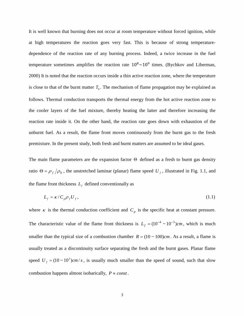
1) At the early stages of flame burning at the closed tube end, the flame front acquires a

finger-shape and demonstrates strong acceleration during a short time interval (Bychkov et

al., 2007; Valiev et al., 2013). As illustrated in Fig. 1.2, the acceleration is terminated as

soon as the flame front touches the side wall of the tube. While, for relatively slow

hydrocarbon flames, this preliminary finger-flame acceleration ends with formation of the

well-known “tulip flame” structure with little relation to DDT; for fast (e.g, hydrogen-

oxygen) flames even short-term finger-flame acceleration increase the flame propagation

speed up to sonic values with important influence on the subsequent DDT process.

7

FIG. 1.2. Evolution of a finger flame front (Bychkov et al., 2007)

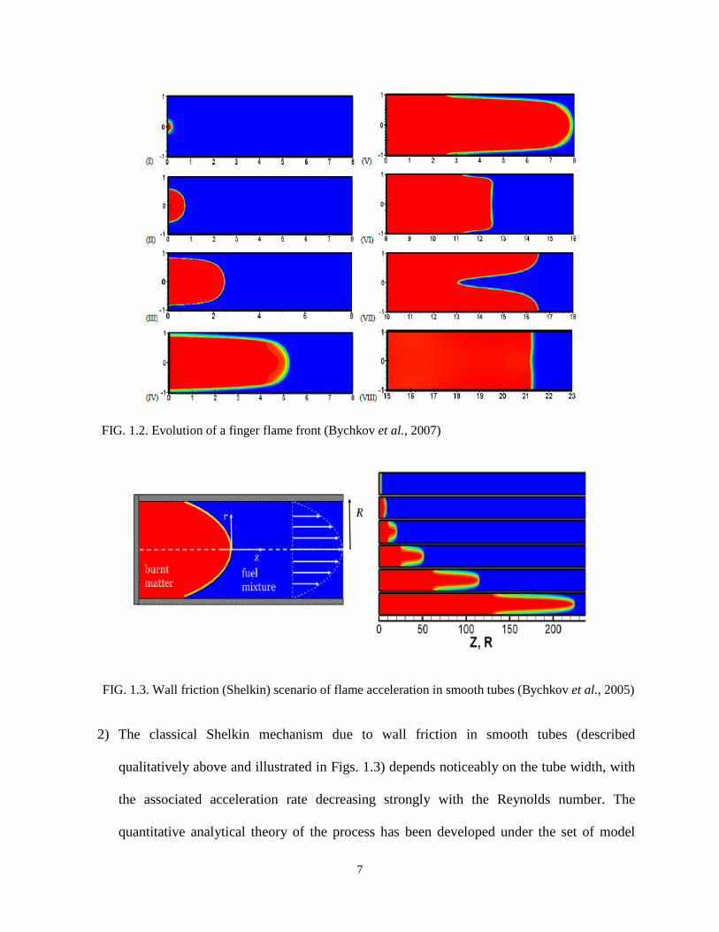
FIG. 1.3. Wall friction (Shelkin) scenario of flame acceleration in smooth tubes (Bychkov et al., 2005)

2) The classical Shelkin mechanism due to wall friction in smooth tubes (described

qualitatively above and illustrated in Figs. 1.3) depends noticeably on the tube width, with

the associated acceleration rate decreasing strongly with the Reynolds number. The

quantitative analytical theory of the process has been developed under the set of model

8

assumptions such as (i) near-isobaric, infinitely thin flame front; (ii) plane-parallel flame

generated flow, (iii) exponential state of the flame acceleration. The theory was validated

by extensive numerical simulations (Bychkov et al., 2005; Akkerman et al., 2006;

Akkerman et al., 2010). These theoretical achievements have also been supported by

refined experiments of the new type on DDT in microtubes (Wu et al., 2007; Wu and

Wang 2011). The success of the theory, being in agreement with the modeling and

experiments, has opened new technological possibilities of DDT in micro-combustion.

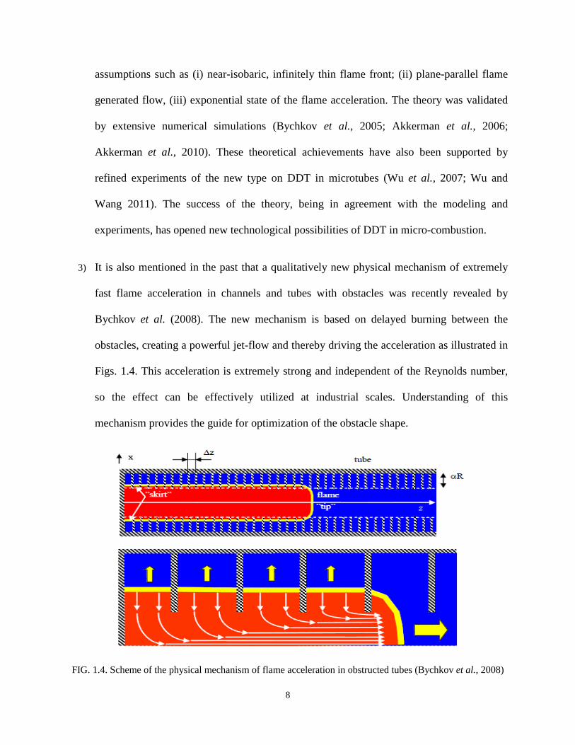
3) It is also mentioned in the past that a qualitatively new physical mechanism of extremely

fast flame acceleration in channels and tubes with obstacles was recently revealed by

Bychkov et al. (2008). The new mechanism is based on delayed burning between the

obstacles, creating a powerful jet-flow and thereby driving the acceleration as illustrated in

Figs. 1.4. This acceleration is extremely strong and independent of the Reynolds number,

so the effect can be effectively utilized at industrial scales. Understanding of this

mechanism provides the guide for optimization of the obstacle shape.

FIG. 1.4. Scheme of the physical mechanism of flame acceleration in obstructed tubes (Bychkov et al., 2008)

9

1.2.2. Objectives

The general goal of this thesis is to shed the light on a set of phenomena within the deflagration

to detonation transition (DDT) scenario. Analytical formulations (Bychkov et al., 2005;

Akkerman et al., 2006) describe the acceleration of a premixed flame propagating in a horizontal

micro channel/tube from its closed end to open one. Whenever, a new theory is proposed, it is

important to know any intrinsic limitations given by associated approximations, and it is critical

to scrutinize the accuracy of the developed theory. In this thesis, these limitations will be

identified and the original formulations will be revised. On the way to this goal, the following

objectives will be met:

• Determine the intrinsic limitations and accuracy of the developed theories of

Bychkov and Akkerman

• Investigate the effect of thermal expansion on flame shape and acceleration

utilizing direct numerical simulations (DNS) and compare the simulation results

with analytical formulations

• By means of DNS, bridge the gap between the theoretical and experimental

studies on ethylene/oxygen combustion (Wu and Wang, 2011)

10

Chapter 2: Theory of Flame Acceleration in Tubes due to Wall

Friction: Intrinsic Limitations and Accuracy

This Chapter is devoted to the model investigation of the near-isobaric flame acceleration in

tubes and channels. Specifically, in Section 2.1, the Bychkov-Akkerman formulation (Bychkov

et al., 2005; Akkerman et al., 2006) is briefly summarized; the intrinsic limitations of this theory

in a 2D geometry are determined in Sec. 2.2,; the findings are extended to the configuration of a

cylindrical pipe in Sec. 2.3, with a quantitative analyses presented in Sec. 2.4. It is emphasized

that the approach of an incompressible flow is adopted in Chapter 2; the effect of gas

compression on the near-sonic flame propagation will be discussed later in Chapter 5.

2.1. Basics of the Bychkov-Akkerman formulation

First of all, the basics of the incompressible analytical theories (Bychkov et al., 2005; Akkerman

et al., 2006) devoted to the 2D and cylindrically-axisymmetric configurations, respectively. The

original formulation is based on the following major approximations:

(i) Near-isobaric combustion process;

(ii) Zero flame thickness;

(iii) Plane-parallel flame-generated flow in the unburned gas, , with the burnt

gas being at rest; and

(iv) Exponential state of the flame acceleration.

Specifically, an infinitely thin premixed laminar flame front that spreads locally with the normal

velocity with respect to the fuel mixture is considered. Such a flame propagates in a 2D

channel of half-width or a cylindrical tube of radius , with adiabatic ( ) non-slip

),( truzzeu =

fU

R R 0=∇⋅ Tn

11

( ) walls, where is a normal vector at the wall. One end of the tube/channel is closed, and

the flame propagates from the closed end to the open one, as illustrated in Fig. 2.1.

FIG. 2.1. A flame in a tube or channel with non-slip at the walls

To simplify the calculations, the standard dimensionless variables , ,

are introduced. The density and pressure are scaled by the fuel quantities and

, respectively. The temperature is scaled by that associated with the fuel, ,

, with and in the fresh and burnt gases, respectively. The average molar

weights of the unburned and burnt gases are assumed to be equal such that the expansion factor

is also associated with the fresh to burnt gas density ratio . Viscosity effects are

characterized by the Reynolds number related to the flame propagation, , where

is the kinematical viscosity.

A traditional evaluation that the total burning rate is simply proportional to the total surface area

of the flame front is employed. In a 2D geometry it reads , and a 2D

“volume” of the burning gas increases by per unit time. In a cylindrical geometry

0=u n

Rzx /);();( =ξη RtU f /=τ

fU/uw = fρ

2ff Uρ fTT /=ϑ

Θ≤≤ ϑ1 1=ϑ Θ=ϑ

Θ bf ρρ=Θ

ν/Re RU f= ν

RSUU Dfw 2// 2=

wRU2)1( −Θ

z

r

α

R

burnt matter

fuel mixture

12

it is calculated as , with a volumetric increment of the burnt gas per unit

time being . In both configurations, the average combustion-generated flow

velocity is related to the total burning rate as

, or , (2.1)

where the scaled total burning rate is adopted.

Obviously, the flow of the fuel mixture in a tube/channel is non-uniform. Indeed, the gas stops at

the non-slip walls because of friction and reaches the maximal velocity at the tube axis. Such a

flow distorts the flame shape, increases the flame surface area and propagation speed. According

to Eq. (2.1), this renders an additional increase of the flow velocity. Consequently, one arrives at

a positive flow-flame feedback: the faster the flow, the stronger the distortion of the flame shape,

and the larger the flame velocity. Therefore, the flame accelerates. Asymptotically, it accelerates

exponentially in time

, , (2.2)

where the dimensionless growth rate is an eigenvalue that will be determined below.

The model of a plane-parallel, flame-generated flow is self-consistent if the pressure gradient is a

function of time only, . Then the plane-parallel Navier-Stokes equation reads

(a), or (b). (2.3)

in a 2D and cylindrical-axisymmetric configurations, respectively, with .

The flame surface is described by a dimensionless function ),()(),( τηττηξ fg += , where

quantifies the evolution of the flame tip and describes the flame shape with respect to it, i.e.

22// RSUU cylfw π=

wUR22)1( π−Θ

wz Uu )1( −Θ= wzw Ω−Θ= )1(

fww UU /=Ω

)/exp( RtUU fw σ∝ )exp(στ∝Ωw

σ

)(/ τξ Π=∂∂p

2

2

Re1)(

ητ

τ ∂∂

+Π=∂

∂ zz ww

∂∂

∂∂

+Π=∂∂

ηη

ηητ

τzz ww 1

Re1)(

( )σττ exp)( ∝Ω∝Π w

g

f

13

the deviation of the flame shape from the planar one. Consequently, every local segment of the

flame front propagates with the velocity in the -direction with

respect to the fuel mixture, with and . In addition, both the flame and the

fuel are drifted by the flame-generated flow, Eq. (2.1). As a result, the flame evolution equation

reads

( ) ( )τητη

τητ∂∂

−∂∂

≈∂∂

−−

∂∂

+=−ffffww zz 11,,0

2

. (2.4)

Equations (2.1) – (2.4) state the backbone of the formulations (Bychkov et al., 2005; Akkerman

et al., 2006; Akkerman et al., 2010).

2.2. Flame acceleration in a 2D channel

Here it is focused on a 2D geometry. The system (2.1), (2.2), (2.3a) has the solution

, (2.5)

( ) ( )στµ

µµµ exp1coshsinhcosh1

1

−−

∝Ω−Θ=−

wzw , (2.6)

where Reσµ = . The flame shape is searched in the form , with

. Then Eqs. (2.4), (2.5) and (2.6) yield (Bychkov et al., 2005)

. (2.7)

With the boundary condition at , Eq. (2.7) acquires the form

. (2.8)

( ) ( )2/1, ητη ∂∂+= fw f ξ

( ) 1,0 =τfw wfw Ω=

µµµµηµ

sinhcosh)cosh(cosh)1( 1−−

−Ω−Θ= wzw

)exp()(),( στητη Φ=f

( ) 00 =Φ

−

−−

+−−

−+−

Φ−Θ=Φ − σσ

σησµ

µσµ

µησµ

µηµµµ

1)exp()(2)exp(

)(2)exp(

sinhcosh)1()1(

22

2

1

)1()( Φ=Φ η 1=η

σσσ

σµµ

σµµ

σµµ

µµµµ 1)exp(

)(2)exp(

)(2exp

)1(sinhcosh

22

2

−−

−+

−−

−+

=−Θ−

14

Equation (2.8) is the major result of the incompressible 2D formulation (Bychkov et al., 2005): it

couples the flame acceleration rate σ to the thermal expansion factor and the flame

propagation Reynolds number , through the intermediate parameter .

The study (Bychkov et al., 2005) moved further: in the limit of large , the leading-order

reduction of Eq. (2.8) can be solved analytically. Indeed, as verified below, a large

corresponds to a large , and for Eq. (2.8) reduces to

, (2.9)

with the solution

, . (2.10)

For large Reynolds numbers, , the result (2.10) further degenerates to ,

. It is seen now that the approach of large and intrinsically requires to be large

as well.

It is emphasized that Eq. (2.10) is based on the assumption of . What does this actually

mean, and what physical parameters would obey this criterion? Of course, one can formally

verify the validity of the theory by computing and , Eq. (2.10), for any given and Re,

and subsequently conclude if such a value of is really large or not. However, the very concept

of needs some quantification as well. Indeed, which is “large enough”: 5, 10, 50, 250,

1000 or larger? Moreover, how does the violation of the limit of large influence the accuracy

of the model? Does this mean that the case of or, say, surely breaks the entire

approach (Bychkov et al., 2005) or not necessarily? Besides, it is realized that the dependences

bf ρρ /=Θ

ν/Re fRU= Reσµ =

Θ

Θ

µ 1>>µ

1)1(

−−Θ=+

µµσµ

2

2

2

1)1(Re

Re41Re4

)1(Re

−

−Θ

+−

=σ

−

−Θ

+−

== 1)1(Re

Re412

1ReRe 2σµ

Θ>> 4Re Re/2Θ=σ

Θ=µ µ Re Θ

1>>µ

σ µ Θ

µ

1>>µ µ

µ

1~µ 5~µ

15

of versus and can demonstrate different trends in terms of the accuracy limitations. So

far, the asymptotical result (2.10) used to be validated by direct numerical simulations (Bychkov

et al., 2005). While the results of these simulations agreed with Eq. (2.10) very well, such

agreement was quite expected since the simulations were performed in the domain of large Re

and , yielding . Would it be the case otherwise?

Furthermore, a comparison to a “computational experiment” cannot be treated as a rigorous

mathematical validation of an analytical theory. As a result, the primary task of this part of the

thesis is to determine the intrinsic limitations and accuracy of the theory above, in general, and

Eq. (2.10), in particular. For this purpose, Eq. (2.8) has been solved computationally, and the

detailed comparison of the results obtained to the prediction of formula (2.10) has been done. A

MATLAB® program was written to solve Eq. (2.8) for the flame acceleration rate numerically.

The program utilizes the Newton-Raphson method – a standard powerful method to solve

equations numerically, which are hard to be solved analytically. (See appendix A for details)

It is recalled in this respect that Eq. (2.8) is also based on a set of model assumptions; see Sec.

2.1. Nevertheless, it is a much less speculative equation as compared to Eq. (2.10) since Eq. (2.8)

does not require any limitations on the physical quantities Re and .

This numerical solution to Eq. (2.8) is compared to the analytical prediction of (2.10) in Fig. 2.2.

Specifically, Fig. 2.2 shows the acceleration rate σ versus the flame propagation Reynolds

number Re at the fixed thermal expansion coefficients 10;8;6;4=Θ . Equations (2.8) and (2.10)

are presented by the dashed and solid lines, respectively.

µ Θ Re

Θ 1>>µ

Θ

16

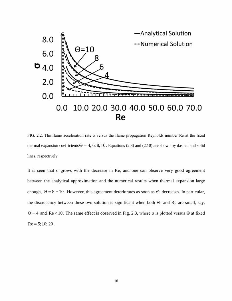
FIG. 2.2. The flame acceleration rate σ versus the flame propagation Reynolds number Re at the fixed

thermal expansion coefficients 10;8;6;4=Θ . Equations (2.8) and (2.10) are shown by dashed and solid

lines, respectively

It is seen that σ grows with the decrease in Re, and one can observe very good agreement

between the analytical approximation and the numerical results when thermal expansion large

enough, . However, this agreement deteriorates as soon as Θ decreases. In particular,

the discrepancy between these two solution is significant when both and Re are small, say,

4=Θ and 10Re < . The same effect is observed in Fig. 2.3, where σ is plotted versus Θ at fixed

20;10;5Re = .

10~8=Θ

Θ

17

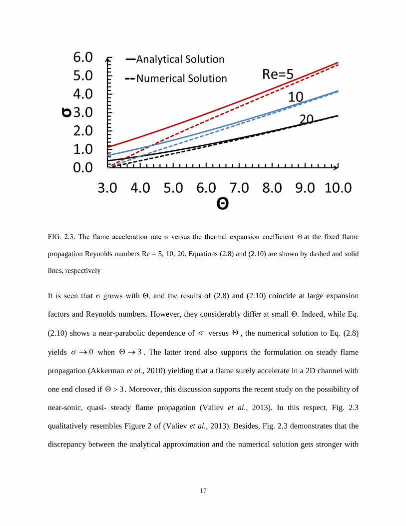
FIG. 2.3. The flame acceleration rate σ versus the thermal expansion coefficient Θ at the fixed flame

propagation Reynolds numbers Re = 5; 10; 20. Equations (2.8) and (2.10) are shown by dashed and solid

lines, respectively

It is seen that σ grows with Θ, and the results of (2.8) and (2.10) coincide at large expansion

factors and Reynolds numbers. However, they considerably differ at small Θ. Indeed, while Eq.

(2.10) shows a near-parabolic dependence of versus , the numerical solution to Eq. (2.8)

yields when . The latter trend also supports the formulation on steady flame

propagation (Akkerman et al., 2010) yielding that a flame surely accelerate in a 2D channel with

one end closed if 3>Θ . Moreover, this discussion supports the recent study on the possibility of

near-sonic, quasi- steady flame propagation (Valiev et al., 2013). In this respect, Fig. 2.3

qualitatively resembles Figure 2 of (Valiev et al., 2013). Besides, Fig. 2.3 demonstrates that the

discrepancy between the analytical approximation and the numerical solution gets stronger with

σ Θ

0→σ 3→Θ

18

the decrease in the flame propagation Reynolds number, and thereby one cannot expect a good

predictability from the theory (Bychkov et al., 2005) at small Re.

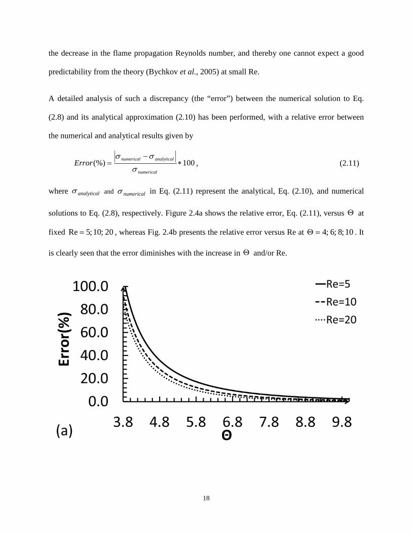
A detailed analysis of such a discrepancy (the “error”) between the numerical solution to Eq.

(2.8) and its analytical approximation (2.10) has been performed, with a relative error between

the numerical and analytical results given by

, (2.11)

where and in Eq. (2.11) represent the analytical, Eq. (2.10), and numerical

solutions to Eq. (2.8), respectively. Figure 2.4a shows the relative error, Eq. (2.11), versus at

fixed , whereas Fig. 2.4b presents the relative error versus Re at . It

is clearly seen that the error diminishes with the increase in and/or Re.

100(%) ∗−

=numerical

analyticalnumericalErrorσ

σσ

analyticalσ numericalσ

Θ

20;10;5Re = 10;8;6;4=Θ

Θ

19

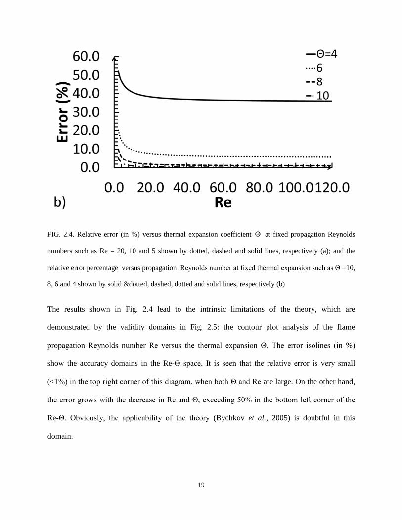
FIG. 2.4. Relative error (in %) versus thermal expansion coefficient Θ at fixed propagation Reynolds

numbers such as Re = 20, 10 and 5 shown by dotted, dashed and solid lines, respectively (a); and the

relative error percentage versus propagation Reynolds number at fixed thermal expansion such as Θ =10,

8, 6 and 4 shown by solid &dotted, dashed, dotted and solid lines, respectively (b)

The results shown in Fig. 2.4 lead to the intrinsic limitations of the theory, which are

demonstrated by the validity domains in Fig. 2.5: the contour plot analysis of the flame

propagation Reynolds number Re versus the thermal expansion Θ. The error isolines (in %)

show the accuracy domains in the Re-Θ space. It is seen that the relative error is very small

(<1%) in the top right corner of this diagram, when both Θ and Re are large. On the other hand,

the error grows with the decrease in Re and Θ, exceeding 50% in the bottom left corner of the

Re-Θ. Obviously, the applicability of the theory (Bychkov et al., 2005) is doubtful in this

domain.

20

FIG. 2.5. Contour scheme (the error isolines (in %)) demonstration of Propagation Reynolds number

versus thermal expansion Θ

2.3. Flame acceleration in a cylindrical tube

In the cylindrical axisymmetric geometry (Akkerman et al., 2006), the counterpart of Eqs. (2.5)

and (2.6) reads

( ) ( ) ( )( ) ( )µµµ

µηµ

11

0

00

21

IIII

w wz −−−

Ω−Θ= , ( ) ( ) ( )( ) ( )στµ

µηµexp

11

0

00

−−

∝Ω−Θ=I

IIw wz , (2.12)

where and ( )µ1I are the modified Bessel function of 0th and 1st orders. Similar to Sec. 2.3,

the flame shape is searched in the form . The cylindrical-axisymmetric

equation for ( )ηΦ is

, (2.13)

with the solution

)(0 ηI

)exp()(),( στητη Φ=f

( ) ( ) ( ) ( )( ) ( )µµµ

µηχχσ

11

0

01

0 21

112II

Id −−

−

Φ−Φ−Θ=Φ′+Φ ∫

21

, . (2.14)

Eventually, the result (2.14) yields

. (2.15)

In the 0th order approximation of : ( ) ( ) ,2/exp10 πµµµµ ≈≈ II ( ) ( ) πµηµηµη 2/exp0 ≈I ,

and Eq. (14) reduces to (Akkerman et al., 2006), with the analytical solution

, . (2.16)

For , Eq.(2.16) further degenerates to , .

Equation (2.15) has been solved computationally in the same manner as Eq. (2.8). Figure 2.6a

shows σ versus Re at fixed 8;6;4=Θ . The computational solution to Eq. (2.15) and the

analytical prediction (2.16) are presented by the dashed and solid lines, respectively. As

expected, the acceleration intensifies with the increase in Θ and the decrease in Re; and in the

cylindrical-axisymmetric configuration the acceleration rate is almost thrice higher the 2D one

for the same parameters. It is shown that while solid and dashed lines qualitatively resemble each

other, the quantitative agreement between them is quite poor. Moreover, unlike Sec. 2.3, the

discrepancy between these two solutions gets much stronger when Re~100. Accordingly, the

same effects are seen in Fig. 2.6b, where σ is plotted versus Θ at fixed .

( ) ( )[ ] ( )[ ] ( ) 1exp1)1(

1exp1)(1−−+Ψ−−+Ψ

Φ=Φσσσηηση ( ) ( )∫=Ψ

η

χσχµχη0

0 exp)( dI

( ) ( )( )

( ) ( ) ( ) ( )∫ −Ψ−−Ψ+−−+

=−Θ

− − 1

02

11

0 exp)(exp)1(1exp112

2ησηησ

σσσµµµ

dII

1−µ

( )1200 −Θ=+ σµ

( )

−

−Θ+= 1

Re181

2Re

0µ ( ) 220

0 1Re

1814

ReRe

−

−Θ+==

µσ

( )18Re −Θ>> ( )120 −Θ=µ ( ) µσ <<−Θ= Re14 20

20;10;5Re =

22

FIG. 2.6. σ versus Re at 8;6;4=Θ (a), and versus Θ at Re = 5; 10; 20 (b). Equations (2.15) and (2.16)

are shown by dashed and solid lines, respectively

Similar to Sec. 2.3, the difference between the numerical solution and the analytical approach is

quantified in Fig. 2.7. Specifically, Fig. 2.7a shows the relative error, given by Eq. (2.11), versus

23

Θ at , while Fig. 2.7b presents the relative error versus Re at 6;4;3=Θ . It is seen

that agreement between the numerical solution and the 0th order approximation is quite poor

everywhere.

FIG. 2.7. The relative error (in %), Eq. (2.11), versus at Re = 5, 10, 20, shown by solid, dashed and

dotted lines, respectively (a); and versus Re at Θ = 3, 4, 6 shown by solid, dashed and dotted lines,

respectively (b)

20;10;5Re =

Θ

24

The results shown in Fig. 2.7 provide the intrinsic limitations of Eq. (2.16) in the Re-Θ diagram,

Fig. 2.8, which represents the counterpart of Fig. 2.5 for the cylindrical configuration, with the

analytical prediction given by the 0th order approximation, Eq. (2.16). The error isolines (in %)

show the accuracy domains in the Re-Θ space. It is seen that even both Re and Θ are large, the

error is still very high: from ~ 24% in the bottom right corner of the diagram till >34% in the top

left corner. Consequently, the quantitative applicability of Eq. (2.16) is very questionable.

FIG. 2.8. Contour scheme (the error isolines (in %)) demonstration in the Re-Θ diagram

Next, it is demonstrated that the analytical prediction can be improved, substantially, if the

formulation is extended to the 1st order approximation of , namely

. (2.17)

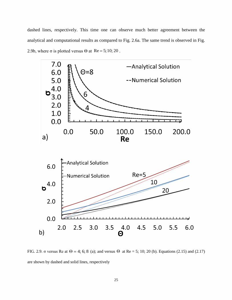
Fig. 2.9 compares Eq. (2.17) and the numerical solution to Eq. (2.15). Specifically, Fig. 2.9a

presents σ versus Re at 8;6;4=Θ . Equations (2.15) and (2.17) are shown by the solid and

11 <<−µ

( )( )

2

0001 1

2111

Re181

4Re

−

+

++−Θ

+=σµµ

σ

25

dashed lines, respectively. This time one can observe much better agreement between the

analytical and computational results as compared to Fig. 2.6a. The same trend is observed in Fig.

2.9b, where σ is plotted versus Θ at .

FIG. 2.9. σ versus Re at 8;6;4=Θ (a); and versus Θ at Re = 5; 10; 20 (b). Equations (2.15) and (2.17)

are shown by dashed and solid lines, respectively

20;10;5Re =

26

Nevertheless, while very good agreement between Eqs. (2.15) and (2.17) is evident at large Θ

and Re, the discrepancy between them gets stronger with the decrease in these parameters and

thereby deteriorates the quantitative predictability of the theory; while Eq. (2.17) yields a near-

parabolic dependence of versus , according to Eq. (2.15), when . Again, the

latter trend reduces the gap between the present theory and the formulation on steady flame

propagation of Akkerman et al., 2010 yielding that a flame surely accelerate in an axisymmetric

configuration with one end closed if ˃ 2.

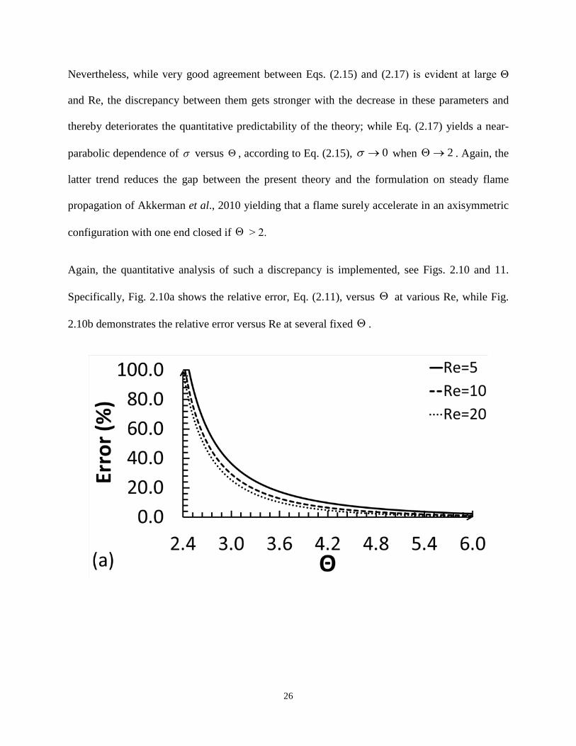
Again, the quantitative analysis of such a discrepancy is implemented, see Figs. 2.10 and 11.

Specifically, Fig. 2.10a shows the relative error, Eq. (2.11), versus at various Re, while Fig.

2.10b demonstrates the relative error versus Re at several fixed .

σ Θ 0→σ 2→Θ

Θ

Θ

Θ

27

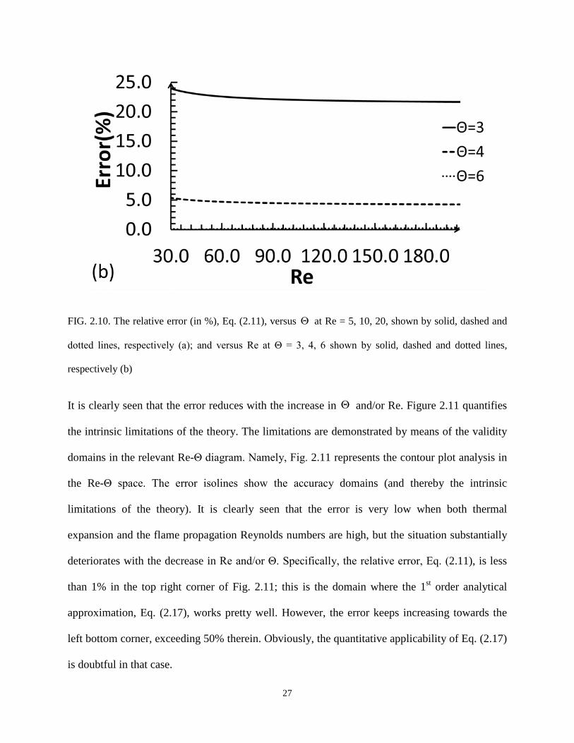
FIG. 2.10. The relative error (in %), Eq. (2.11), versus at Re = 5, 10, 20, shown by solid, dashed and

dotted lines, respectively (a); and versus Re at Θ = 3, 4, 6 shown by solid, dashed and dotted lines,

respectively (b)

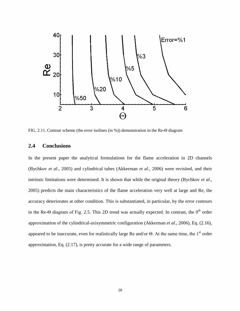
It is clearly seen that the error reduces with the increase in and/or Re. Figure 2.11 quantifies

the intrinsic limitations of the theory. The limitations are demonstrated by means of the validity

domains in the relevant Re-Θ diagram. Namely, Fig. 2.11 represents the contour plot analysis in

the Re-Θ space. The error isolines show the accuracy domains (and thereby the intrinsic

limitations of the theory). It is clearly seen that the error is very low when both thermal

expansion and the flame propagation Reynolds numbers are high, but the situation substantially

deteriorates with the decrease in Re and/or Θ. Specifically, the relative error, Eq. (2.11), is less

than 1% in the top right corner of Fig. 2.11; this is the domain where the 1st order analytical

approximation, Eq. (2.17), works pretty well. However, the error keeps increasing towards the

left bottom corner, exceeding 50% therein. Obviously, the quantitative applicability of Eq. (2.17)

is doubtful in that case.

Θ

Θ

28

FIG. 2.11. Contour scheme (the error isolines (in %)) demonstration in the Re-Θ diagram

2.4 Conclusions

In the present paper the analytical formulations for the flame acceleration in 2D channels

(Bychkov et al., 2005) and cylindrical tubes (Akkerman et al., 2006) were revisited, and their

intrinsic limitations were determined. It is shown that while the original theory (Bychkov et al.,

2005) predicts the main characteristics of the flame acceleration very well at large and Re, the

accuracy deteriorates at other condition. This is substantiated, in particular, by the error contours

in the Re-Θ diagram of Fig. 2.5. This 2D trend was actually expected. In contrast, the 0th order

approximation of the cylindrical-axisymmetric configuration (Akkerman et al., 2006), Eq. (2.16),

appeared to be inaccurate, even for realistically large Re and/or Θ. At the same time, the 1st order

approximation, Eq. (2.17), is pretty accurate for a wide range of parameters.

29

Chapter 3: Computational Platform

A fully-compressible, finite-volume Navier–Stokes “in-house” solver of Dr. Akkerman’s group

at West Virginia University has been used as the major computational platform of this work. The

embryo of this code was developed originally by Dr. Lars-Erik Eriksson at Volvo Aero

Company (Goteborg, Sweden), and it was subsequently updated, comprehensively, by several

research groups, including the group of Prof. M. Liberman at Uppsala University as well as that

of Prof. V. Bychkov at Umea University, both in Sweden, and eventually the group of Dr.

Akkerman. One of the active developers of this computational platform is Dr. Damir Valiev,

who is currently affiliated with Sandia National Laboratories and Princeton University.

The code solves the complete set of the hydrodynamic and combustion equations including

transport processes (diffusion, viscosity, heat conduction) and the Arrhenius chemical kinetics.

The numerical scheme is second order accurate in time, fourth order in space for the convective

terms, and second order in space for the diffusive term. The solver is robust and accurate, having

been successfully utilized in numerous aero-acoustic and combustion applications (Erikkson,

1987; Erikkson, 1995; Anderson et al., 2005; Wollblad et al., 2006). It is adapted for parallel

computations and available in 2D (Cartesian and cylindrical axisymmetric) version, as well as

fully 3D Cartesian version, with a self-adaptive structured computational grid employed that

makes the code perfect, in particular, for fundamental studies of flame hydrodynamics in

combustion tubes, chambers as well as for outwardly-propagating flames in free space.

3.1 Governing equations

In the general form, the complete set of the governing equations of compressible hydrodynamic

and combustion include: the continuity equation,

30

( ) ( ) 01=

∂∂

+∂∂

+∂∂

zr uz

urrrt

ρρρ ββ , (3.1)

the Navier-Stokes (momentum) equation,

( ) ( )[ ] ( ) 01,

2, =Ψ+

∂∂

+−∂∂

+−∂∂

+∂∂

ββ

β ζρζρρrPu

zuur

rru

t zzzrzrzz (3.2a)

( ) ( )[ ] ( ) 01,,

2 =Ψ+∂∂

+−∂∂

+−∂∂

+∂∂

ββ

β ζρζρρrPuu

zur

rru

t zrzrrrrr , (3.2b)

the energy balance equation,

( )( )[ ]++−−+∂∂

+∂∂

rzzrrrrr quuuPrrrt ,,

1 ζζεε ββ

( )[ ] 0,, =+−−+∂∂

zrzrzzzz quuuPz

ζζε , (3.3)

and the species equation,

( ) ( )TREYzYYu

zrYYur

rrY

t paR

zi −−=

∂∂

−∂∂

+

∂∂

−∂∂

+∂∂ exp

ScSc1

τρµρµρρ γ

γ (3.4)

where 0=β and 1 for 2D and axisymmetric geometries respectively,

( ) ( )22

2 rzV uuTCQY +++=ρρε , (3.5)

is the total energy per unit volume, Y the mass fraction of the fuel, Q the energy release from

the reaction, and VC the heat capacity at constant volume. The energy diffusion vector iq is

given by

∂∂

+∂∂

−=rYQ

rTCq P

r ScPrµ , (3.6)

∂∂

+∂∂

−=zYQ

zTCq P

z ScPrµ . (3.7)

The stress tensor ji,ζ takes the form

31

∂∂

−∂

∂+

∂∂

= jik

k

i

j

j

iji x

uxu

xu

,, 32 δµζ (3.8)

in the 2D configuration ( 0=β ), while in the axisymmetric geometry ( 1=β ) it reads

−

∂∂

−∂∂

=r

uz

ur

u rzrrr 2

32

,µζ , (3.9)

−

∂∂

−∂∂

=r

ur

uz

u rrzzz 2

32

,µζ , (3.10)

∂

∂+

∂∂

=r

uz

u zrzr µζ , . (3.11)

Finally, the last term in Eq. (3.2) takes the form

∂∂

−∂∂

−=z

ur

ur

u zrr23

2µψ β (3.12)

if 1=β , and 0=βψ if 0=β . Here µ is the dynamic viscosity, Pr and Sc the Prandtl and

Schmidt numbers, respectively. Unburned and burned mixtures are assumed to be ideal two-

atomic gases and have the same molecular weights mmm bf == . Then the specific heats are

mRC pV 2/5= , mRRCC ppVP 2/7=+≡ , and the equation of state reads

mTRP p /ρ= , (3.13)

where ( )KmolJ431.8 ⋅≈PR is the universal gas constant. A one-step irreversible Arrhenius

reaction of the 1st order is typically employed (though the reaction order may vary), with the

activation energy aE and frequency factor corresponding to a characteristic time Rτ . The factor

Rτ is adjusted to obtain a particular value of the unstretched laminar flame speed fU by solving

the associated eigenvalue problem. In other words, the flame velocity is almost fully determined

by the set of chemical parameters of the fuel: aE , Rτ , Q . Compressibility is characterized by the

initial Mach number coupled to the planar flame speed, Sf cUMa /≡ . For typical hydrocarbon

32

deflagrations it is pretty small, 0.001~0.01. In that case, the flow is almost isobaric and thermal

expansion is coupled to the energy release in the burning process as follows

fPfb TCQTT /1+==Θ . (3.14)

The flame thickness is conventionally defined as

f

th

fff U

DU

L ≡≡ρµ

Pr, (3.15)

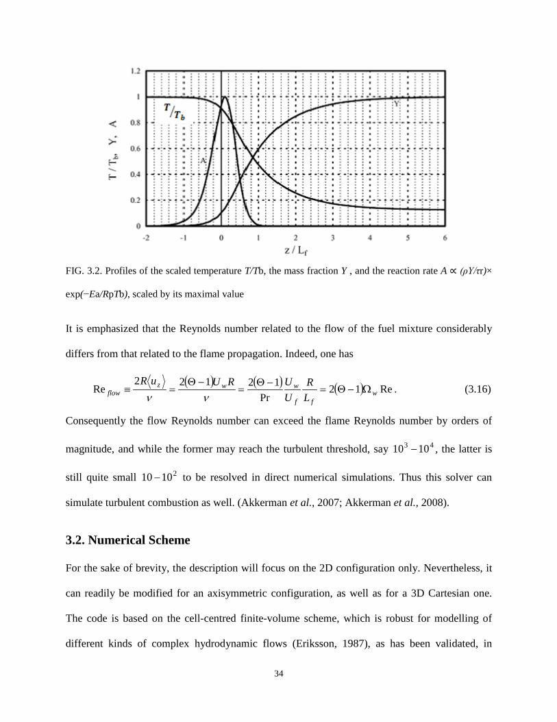
where thD is the thermal diffusivity and Pr is the Prandtl number. It is noted that the quantity

(3.15) is a characteristic parameter of the problem of length dimension, while the real size of the

combustion zone can be several times wider. In a certain sense, fL characterizes the active

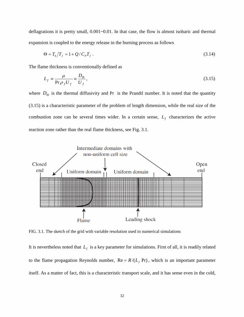
reaction zone rather than the real flame thickness, see Fig. 3.1.

FIG. 3.1. The sketch of the grid with variable resolution used in numerical simulations

It is nevertheless noted that fL is a key parameter for simulations. First of all, it is readily related

to the flame propagation Reynolds number, Pr)/(Re fLR= , which is an important parameter

itself. As a matter of fact, this is a characteristic transport scale, and it has sense even in the cold,

33

non-reacting flow. In addition, the resolution abilities of the solver are given by fL : from 2 to 5

grid points have to be taken per fL to imitate the combustion process properly. The current

version of the solver allows taking up to 5-10 million grid points (cells) on modern clusters,

while RAM problems may appear at larger mesh sizes. Therefore, one can readily determine the

maximal scale that can be resolved for a particular computational configuration.

Mesh with variable resolution is used in order to take into account the growing distances

between the tube end, the accelerating flame and the pressure wave, and to resolve both chemical

and hydrodynamic spatial scales. Typical computation time for one simulation required up to 104

CPU-hours, hence implying the need for extensive parallel calculations. A rectangular grid with

the grid walls parallel to the coordinate axes was used. The sketch of the calculation mesh used

in the simulations of flame acceleration from the closed tube end is shown in Fig. 3.1. To

perform all the calculations in a reasonable time, the grid spacing non-uniform along the z-axis

with the zones of fine grid around the flame and leading shock fronts were established. For the

majority of the simulation runs, the grid size in the z-direction was 0.25 fL and 0.5 fL in the

domains of the flame and leading pressure wave, respectively, which allowed resolution of the

flame and waves. Outside the region of fine grid the mesh size increased gradually with 2%

change in size between the neighboring cells. In order to keep the flame and pressure waves in

the zone of fine grid, the periodical mesh reconstruction during the simulation run (Valiev et al.,

2008) were employed. Third-order splines were used for interpolation of the flow variables

during periodic grid reconstruction to preserve the second order accuracy of the numerical

scheme.

34

FIG. 3.2. Profiles of the scaled temperature T/Tb, the mass fraction Y , and the reaction rate A ∝ (ρY/τr)×

exp(−Ea/RpTb), scaled by its maximal value

It is emphasized that the Reynolds number related to the flow of the fuel mixture considerably

differs from that related to the flame propagation. Indeed, one has

( ) ( ) ( ) Re12Pr

12122Re w

ff

wwzflow L

RUURUuR

Ω−Θ=−Θ

=−Θ

=≡νν

. (3.16)

Consequently the flow Reynolds number can exceed the flame Reynolds number by orders of

magnitude, and while the former may reach the turbulent threshold, say 43 1010 − , the latter is

still quite small 21010 − to be resolved in direct numerical simulations. Thus this solver can

simulate turbulent combustion as well. (Akkerman et al., 2007; Akkerman et al., 2008).

3.2. Numerical Scheme

For the sake of brevity, the description will focus on the 2D configuration only. Nevertheless, it

can readily be modified for an axisymmetric configuration, as well as for a 3D Cartesian one.

The code is based on the cell-centred finite-volume scheme, which is robust for modelling of

different kinds of complex hydrodynamic flows (Eriksson, 1987), as has been validated, in

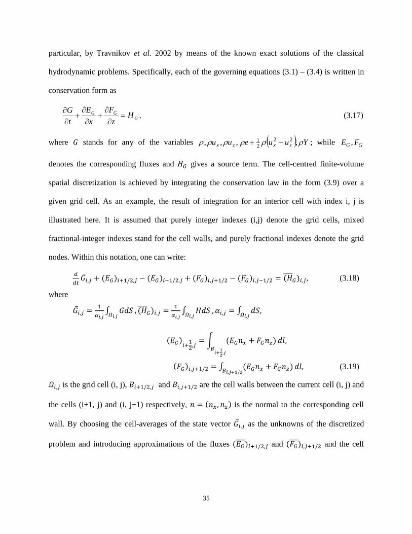
35

particular, by Travnikov et al. 2002 by means of the known exact solutions of the classical

hydrodynamic problems. Specifically, each of the governing equations (3.1) – (3.4) is written in

conservation form as

GGG Hz

Fx

EtG

=∂

∂+

∂∂

+∂∂

, (3.17)

where 𝐺 stands for any of the variables ( ) Yuueuu zxzx ρρρρρρ ,,,, 2221 ++ ; while GG FE ,

denotes the corresponding fluxes and 𝐻𝐺 gives a source term. The cell-centred finite-volume

spatial discretization is achieved by integrating the conservation law in the form (3.9) over a

given grid cell. As an example, the result of integration for an interior cell with index i, j is

illustrated here. It is assumed that purely integer indexes (i,j) denote the grid cells, mixed

fractional-integer indexes stand for the cell walls, and purely fractional indexes denote the grid

nodes. Within this notation, one can write:

𝑑𝑑𝑡𝑖,𝑗 + (𝐸𝐺)𝑖+1/2,𝑗 − (𝐸𝐺)𝑖−1/2,𝑗 + (𝐹𝐺)𝑖,𝑗+1/2 − (𝐹𝐺)𝑖,𝑗−1/2 = (𝐻𝐺)𝑖,𝑗 , (3.18)

where

𝑖,𝑗 = 1𝛼𝑖,𝑗

∫ 𝐺𝑑𝑆 𝛺𝑖,𝑗

, (𝐻𝐺)𝑖,𝑗 = 1𝛼𝑖,𝑗

∫ 𝐻𝑑𝑆 𝛺𝑖,𝑗

,𝛼𝑖,𝑗 = ∫ 𝑑𝑆 𝛺𝑖,𝑗

,

(𝐸𝐺)𝑖+12,𝑗

= (𝐸𝐺𝑛𝑥 + 𝐹𝐺𝑛𝑧)

𝐵𝑖+12,𝑗

𝑑𝑙,

(𝐹𝐺)𝑖,𝑗+1/2 = ∫ (𝐸𝐺𝑛𝑥 + 𝐹𝐺𝑛𝑧) 𝐵𝑖,𝑗+1/2

𝑑𝑙, (3.19)

𝛺𝑖,𝑗 is the grid cell (i, j), 𝐵𝑖+1/2,𝑗 and 𝐵𝑖,𝑗+1/2 are the cell walls between the current cell (i, j) and

the cells (i+1, j) and (i, j+1) respectively, 𝑛 = (𝑛𝑥,𝑛𝑧) is the normal to the corresponding cell

wall. By choosing the cell-averages of the state vector 𝑖,𝑗 as the unknowns of the discretized

problem and introducing approximations of the fluxes (𝐸𝐺)𝑖+1/2,𝑗 and (𝐹𝐺)𝑖,𝑗+1/2 and the cell

36

averaged source vector (𝐻𝐺)𝑖,𝑗+1/2 in terms of these unknowns, the final spatial discretization of

(3.9) can be obtained.

A key feature of the cell-centred finite volume discretization of (3.9) given by (3.10) is the

numerical approximation of the fluxes (𝐸𝐺)𝑖+1/2,𝑗 and (𝐹𝐺)𝑖,𝑗+1/2 in terms of the cell averages

𝑖,𝑗 . The usual approach is to treat the convective flux approximations and the diffusive flux ones

separately due to the different nature of these fluxes. For the convective fluxes, a characteristic-

upwind flux scheme (Eriksson, 1987), where the propagation directions of the various

characteristic variables control a user-given degree of up-winding, is employed. Here it turns out

to be advantageous to work with the hydro-dynamical variables 𝜌, 𝑢𝑥,𝑢𝑧 ,𝑃,𝑌, instead of the

conservative variables in the state vector 𝑖,𝑗. The numerical errors introduced by using this

approximation are of the second order in grid spacing assuming a smooth solution. For problems

where all spatial scales are adequately resolved in the computational grid, an extremely small

amount of up-winding may be used, giving an almost centred scheme with minimal numerical

dissipation and dispersion.

3.3. Principles of setting the initial conditions

a) Planar flame front ignition

The easiest but feasible way to employ the initial conditions for an initially planar premixed

flame front is to approximate it by the classical Zeldochich-Frank-Kamenetsky (ZFK) solution

(Bychkov and Liberman, 2000). In the reference frame co-moving with the flame front it reads

( ) ( ) ( )

<Θ

≥−−Θ+=

0,

0,/exp11

zzLz

TzT f

f

(3.20)

37

( ) ( )( ) ( )

( )

<−Θ

≥−−Θ−=

−

0,1

0,/exp11Pr34

2 zzLz

SPzP f

Lf

f

ρ (3.21)

with

( )

( ) f

f

L

z

TT

zSzu

==ρρ

, ( )1/

−Θ

−Θ= fTT

zY . (3.22)

b) Hemispherical flame front ignition

At the open tube end, the non-reflecting boundary conditions are applied. As initial conditions,

a hemi-spherical (hemi-circular) version of the ZFK solution is used, namely

( )ffbf LzrTTTT /exp)( 22 +−−+= , if 222frxz <+ , (3.23)

fTT Θ= , if 222frxz >+ , (3.24)

)/()( fbb TTTTY −−= , fPP = , 0=xu , 0=zu . (3.25)

Here fr is the radius of initial flame ball at the closed end of the tube. The finite initial radius of

the flame ball is equivalent to a time shift, which required proper adjustments when comparing

the theory and numerical simulations. When necessary, the numerical solution in time is shifted

in order to have the theory and the modeling results starting from the same point.

38

Chapter 4: Effect of Thermal Expansion on Flame Propagation in

Channels with Nonslip Walls: Numerical and Analytical

Consideration

4.1 Motivation

To begin with, it is pointed out that the theories (Bychkov et al., 2005; Akkerman et al., 2006)

include a set of assumptions such as the large Reynolds number related to flame propagation, as

well as the large thermal expansion coefficient in the burning process, which in turn leads to the

intrinsic limitations of the theory. In Chapter 2, these limitations have been determined, and

thereby validity domains of the Bychkov approximation within a Re−Θ diagram were clearly

underlined. Furthermore, the error analysis related to the intrinsic assumptions and accuracy of

the developed theory was also performed.

The main purpose of the present component of this thesis is to substantiate the validity domains

obtained in Chapter 2, in particular, as well as the formulation (Bychkov et al., 2005), in general,

by usage of comprehensive direct numerical simulations for the variety of parameters, in

particular, Θ and Re. The numerical simulations are performed for the complete set of

combustion equations including thermal conduction, viscosity, diffusion and chemical kinetics

with one-step Arrhenius reaction. It is demonstrated that while the simulations fit the theoretical

prediction for large ,Θ a decrease in Θ and a variation of Re lead to the deviation from the

exponential state of acceleration. The planar flame speed is taken to be Uf =30-40 cm/s,

providing a realistically low flame propagation Mach number, ~ 310− , and the thermal expansion

in the burning process was taken in the range of 12~4=Θ , which fits typical hydrocarbon

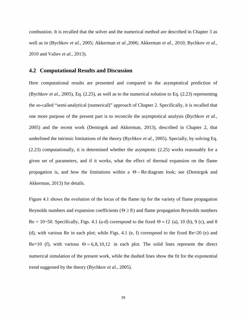
39

combustion. It is recalled that the solver and the numerical method are described in Chapter 3 as

well as in (Bychkov et al., 2005; Akkerman et al.,2006; Akkerman et al., 2010; Bychkov et al.,

2010 and Valiev et al., 2013).

4.2 Computational Results and Discussion

Here computational results are presented and compared to the asymptotical prediction of

(Bychkov et al., 2005), Eq. (2.25), as well as to the numerical solution to Eq. (2.23) representing

the so-called “semi-analytical (numerical)” approach of Chapter 2. Specifically, it is recalled that

one more purpose of the present part is to reconcile the asymptotical analysis (Bychkov et al.,

2005) and the recent work (Demirgok and Akkerman, 2013), described in Chapter 2, that

underlined the intrinsic limitations of the theory (Bychkov et al., 2005). Specially, by solving Eq.

(2.23) computationally, it is determined whether the asymptotic (2.25) works reasonably for a

given set of parameters, and if it works, what the effect of thermal expansion on the flame

propagation is, and how the limitations within a Re−Θ diagram look; see (Demirgok and

Akkerman, 2013) for details.

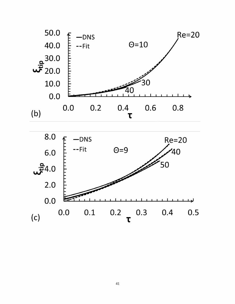
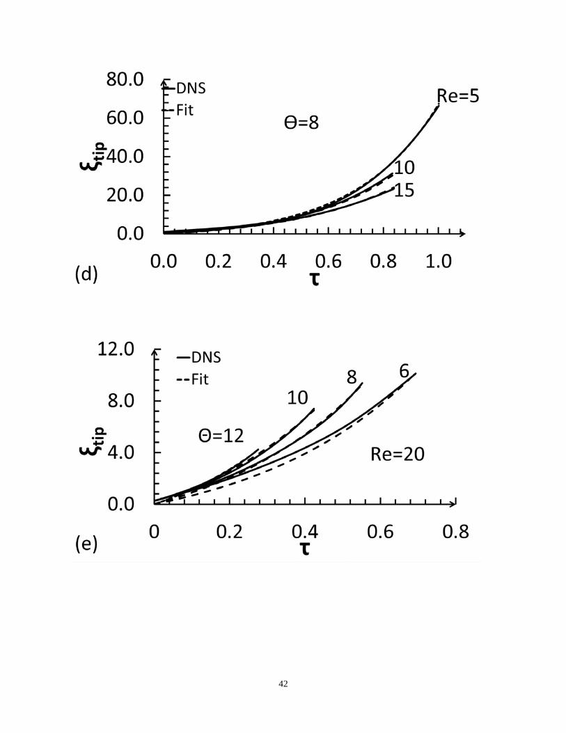
Figure 4.1 shows the evolution of the locus of the flame tip for the variety of flame propagation

Reynolds numbers and expansion coefficients ( 8≥Θ ) and flame propagation Reynolds numbers

Re = 10~50. Specifically, Figs. 4.1 (a-d) correspond to the fixed 12=Θ (a), 10 (b), 9 (c), and 8

(d), with various Re in each plot; while Figs. 4.1 (e, f) correspond to the fixed Re=20 (e) and

Re=10 (f), with various 12,10,8,6=Θ in each plot. The solid lines represent the direct

numerical simulation of the present work, while the dashed lines show the fit for the exponential

trend suggested by the theory (Bychkov et al., 2005).

40

In Figure 4.1 (a-d) one observes very good agreement between the computational and theoretical

results. Indeed, look at the respective solid lines, representing direct numerical simulations, and

the dashed ones, showing an exponential fit suggested by the theory. It is clearly shown that the

respective results coincidence and overlap each other. Also, it can be stated that a flame

propagates faster in a narrower tube. Indeed, this is seen in Fig.4.1a, where two different tubes

are compared at fixed Θ = 12, with the flame propagation Reynolds numbers being 25, 15 and

10, respectively. One can observe that the solution with lower Re exceeds that at higher Re for

the same scaled time instant. Therefore, the flame acceleration rate decreases with the tube

radius.

41

42

43

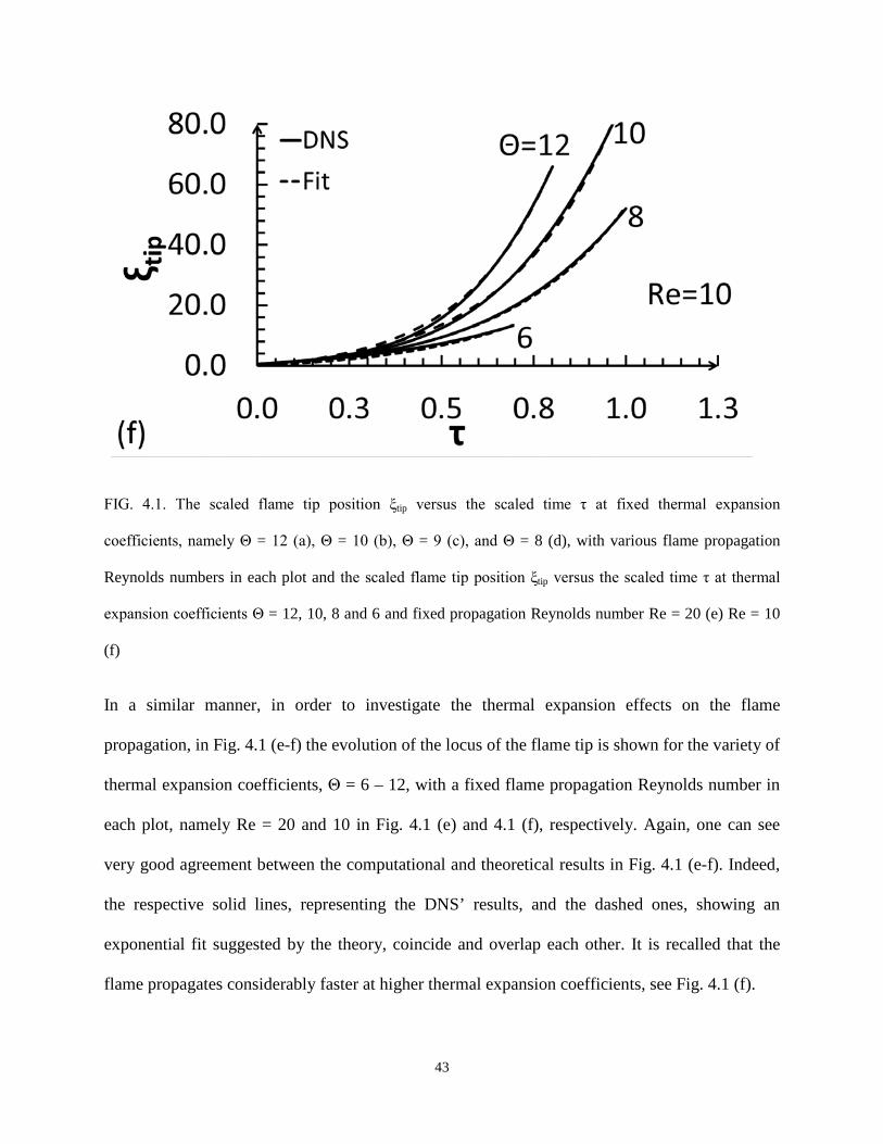
FIG. 4.1. The scaled flame tip position ξtip versus the scaled time τ at fixed thermal expansion

coefficients, namely Θ = 12 (a), Θ = 10 (b), Θ = 9 (c), and Θ = 8 (d), with various flame propagation

Reynolds numbers in each plot and the scaled flame tip position ξtip versus the scaled time τ at thermal

expansion coefficients Θ = 12, 10, 8 and 6 and fixed propagation Reynolds number Re = 20 (e) Re = 10

(f)

In a similar manner, in order to investigate the thermal expansion effects on the flame

propagation, in Fig. 4.1 (e-f) the evolution of the locus of the flame tip is shown for the variety of

thermal expansion coefficients, Θ = 6 – 12, with a fixed flame propagation Reynolds number in

each plot, namely Re = 20 and 10 in Fig. 4.1 (e) and 4.1 (f), respectively. Again, one can see

very good agreement between the computational and theoretical results in Fig. 4.1 (e-f). Indeed,

the respective solid lines, representing the DNS’ results, and the dashed ones, showing an

exponential fit suggested by the theory, coincide and overlap each other. It is recalled that the

flame propagates considerably faster at higher thermal expansion coefficients, see Fig. 4.1 (f).

44

Figure 4.2 presents the flame acceleration rate versus the flame-related Reynolds number, with

different expansion coefficients in each plot. The result resembles indirectly that of Fig.4.1.

Indeed, it is clearly seen from Fig. 4.2 that the solid and dashed lines start deviating from each

other as soon as Θ goes below 8, which yields a certain threshold thermal expansion for the

intrinsic validity of the asymptotic (2.10).

In spite of a certain discrepancy between the results of (2.8) and (2.10) in Figs. 4.2 (e, f), our

numerical simulations demonstrate that, for ,86 <Θ≤ a flame front still may (or may not)

accelerate exponentially depending on other parameters, such as Re. Namely, the exponential

acceleration regime breaks as soon as Re exceeds some threshold value, Re~20, as shown by the

vertical dotted lines in Figs. 4.2 (e, f). As a matter of fact, this effect does not agree with the

main conclusion of Chapter 2 that the asymptotic (2.10) still works more or less fine for

86 <Θ≤ . Moreover (which is much more important!), while Chapter 2 and the study

(Demirgok and Akkerman, 2013) yield that agreement between Eqs. (2.8) and (2.10) improves

with the increase in Re, here the opposite tendency is observed. Without any guarantee that the

following idea is correct, it is hypothesized that such a discrepancy is devoted to additional

effects that might appear in wide tubes, say, the development of the hydrodynamic (Darrieus-

Landau; DL) instability that can modify a self-similar manner of the flame acceleration.

45

46

47

FIG. 4.2. The flame acceleration rate σ versus propagation Reynolds number Re at thermal expansion Θ =

12 (a), 10 (b), 9 (c), 8 (d), 7 (e), 6 (f)

48

It is noted that while one can observe excellent agreement between the results of (2.8), (2.10) and

the DNS when 8≥Θ , such excellent agreement degrades as soon as 8<Θ is taken. Indeed,

agreement is quite limited for ,86 <Θ≤ and one faces no agreement at all (no exponential trend

observed) for .6<Θ

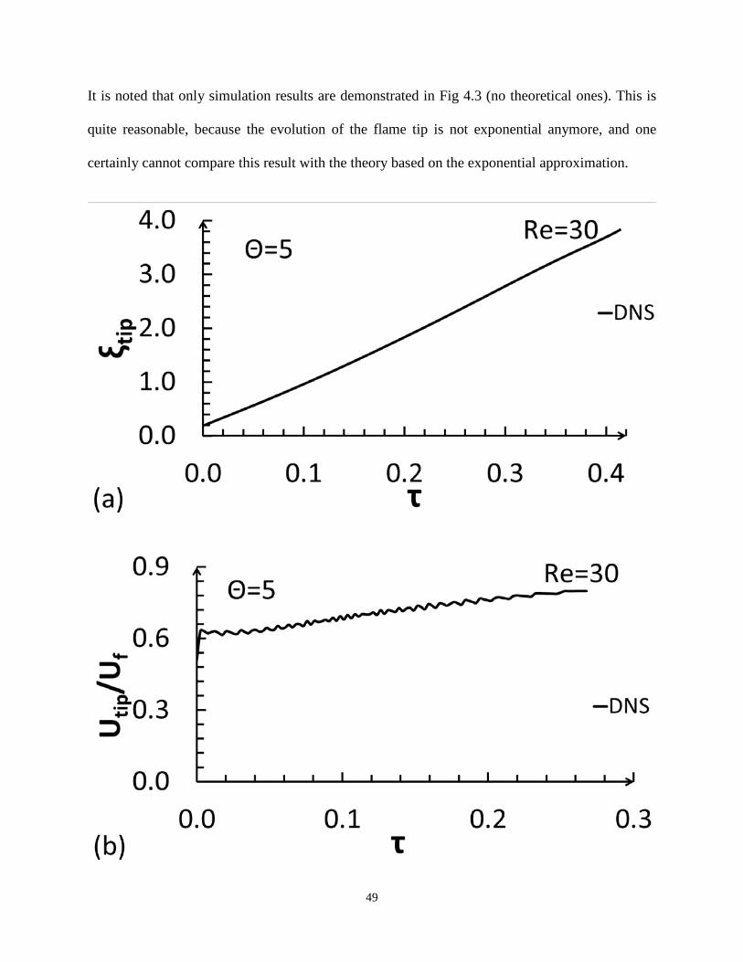
Fig. 4.3a presents the evolution of the locus of the flame tip for the flame propagation Reynolds

number Re = 30 and the expansion coefficient 5=Θ , obtained computationally. Figure 4.3b

shows the scaled flame tip velocity Utip /Uf versus the scaled time τ = t Uf / R at the fixed thermal

expansion coefficient Θ = 5 and the flame propagation Reynolds numbers Re = 30. Here one can

see no agreement with the theory (Bychkov et al., 2005) at all: unlike the theoretical prediction,

no exponential trend is observed in our simulations.

Similarly, the scaled flame tip velocity Utip /Uf in Fig. 4.3b does not fit an exponential trend as

well. Moreover, there are oscillations happening in the evolution of scaled flame velocity. Again,

it is assumed that such a discrepancy is related to additional effects that might appear not only in

wide tubes but also in a combustion process having a low thermal expansion that can somehow

modify a self-similar manner of the flame acceleration.

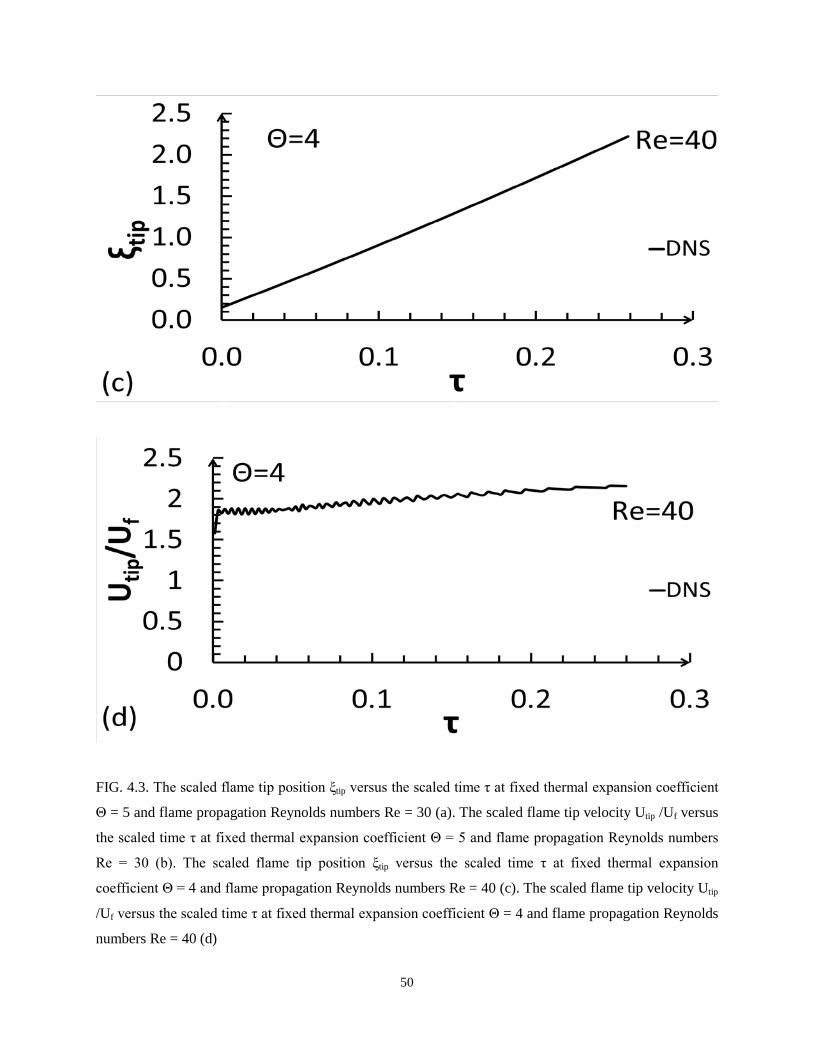
Figures 4.3 (c, d) are the counterparts of Fig. 4.3 (a, b) for Θ = 4. They yield the same result:

neither the evolution of the flame tip position, nor its speed exhibit the exponential accelerative

dynamics. Anyway, as soon as Θ goes below 6, the exponential acceleration in the simulations

is not observed at all, and this qualitatively fits both the original paper (Bychkov et al., 2005) and

its justification (Demirgok and Akkerman, 2013). It is emphasized that the case of 4=Θ

conceptually differs from that of, say, .9=Θ

49

It is noted that only simulation results are demonstrated in Fig 4.3 (no theoretical ones). This is

quite reasonable, because the evolution of the flame tip is not exponential anymore, and one

certainly cannot compare this result with the theory based on the exponential approximation.

50

FIG. 4.3. The scaled flame tip position ξtip versus the scaled time τ at fixed thermal expansion coefficient

Θ = 5 and flame propagation Reynolds numbers Re = 30 (a). The scaled flame tip velocity Utip /Uf versus

the scaled time τ at fixed thermal expansion coefficient Θ = 5 and flame propagation Reynolds numbers

Re = 30 (b). The scaled flame tip position ξtip versus the scaled time τ at fixed thermal expansion

coefficient Θ = 4 and flame propagation Reynolds numbers Re = 40 (c). The scaled flame tip velocity Utip

/Uf versus the scaled time τ at fixed thermal expansion coefficient Θ = 4 and flame propagation Reynolds

numbers Re = 40 (d)

51

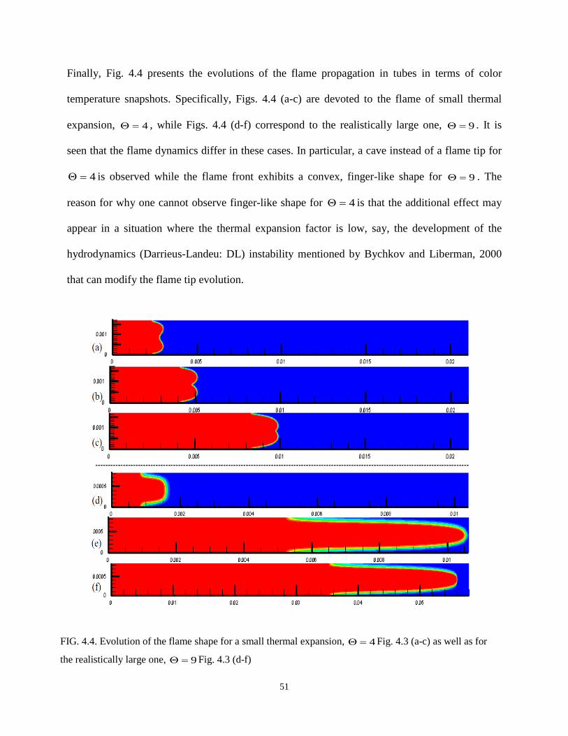
Finally, Fig. 4.4 presents the evolutions of the flame propagation in tubes in terms of color

temperature snapshots. Specifically, Figs. 4.4 (a-c) are devoted to the flame of small thermal

expansion, 4=Θ , while Figs. 4.4 (d-f) correspond to the realistically large one, 9=Θ . It is

seen that the flame dynamics differ in these cases. In particular, a cave instead of a flame tip for

4=Θ is observed while the flame front exhibits a convex, finger-like shape for 9=Θ . The

reason for why one cannot observe finger-like shape for 4=Θ is that the additional effect may

appear in a situation where the thermal expansion factor is low, say, the development of the

hydrodynamics (Darrieus-Landeu: DL) instability mentioned by Bychkov and Liberman, 2000

that can modify the flame tip evolution.

FIG. 4.4. Evolution of the flame shape for a small thermal expansion, 4=Θ Fig. 4.3 (a-c) as well as for

the realistically large one, 9=Θ Fig. 4.3 (d-f)

52

4.3 Conclusions

In this chapter, the analytical (Bychkov et al., 2005), semi-analytical, Chapter 2 and (Demirgok

and Akkerman, 2013), and fully computational (DNS) approaches to flame acceleration in tubes

due to wall friction are reconciled. It is shown that while the theory predicts the main

characteristics of the flame acceleration very well when both Θ and Re are large enough, it may

or may not be as accurate otherwise. In particular, it can be concluded that the theory

quantitatively deteriorates for 86 <Θ≤ , though it still may or may not work qualitatively

(exhibiting the exponential acceleration or not), depending on Re. Finally, the theory breaks as

soon as the expansion factor goes below 6.

53

Chapter 5: Analysis of Ethylene-Oxygen Combustion in Micro-Pipes

Propagation of stoichiometric ethylene-oxygen premixed flames in cylindrical pipes of sub/near-

millimeter radii is investigated computationally and analytically. Then computational and

analytical results are compared to the recent experiments (Wu and Wang, 2011). Namely,

various stages of flame evolution such as quasi-isobaric, exponential acceleration; its moderation

due to gas compression; and eventual saturation to the Chapman-Jouget deflagration are

detected. Specifically, the dynamics and morphology of the flame front, its propagation velocity

and acceleration rate are determined. Due to viscous heating, the entire process can be followed

by the detonation initiation ahead of the flame front. The computational component of this

research is based on the computational platform described in Chapter 3. The overall study

bridges the gap between the experiments (Wu and Wang, 2011) and the analytical formulation

(Akkerman et al., 2006).

5.1 Formulation

Recent experiments have shown the occurrence of acceleration and DDT for ethylene-oxygen

flames in micro-tubes/channels with diameter ~1 mm (Wu and Wang, 2011). However, in

contrast to the theories discussed in Chapter 2, which predict an exponential acceleration of

laminar flames in micro-scale tubes at the initial stage, the experiments demonstrated a number

of specific effects beyond the scope of the incompressible flow adopted in these analyses, such

as moderated flame acceleration with subsequent saturation of the flame velocity to a steady

value, which can be interpreted as the Chapman-Jouguet (CJ) deflagration speed.

To elucidate these observations, in particular, the experiments in micro-tubes, the role of gas

compression has been investigated in the acceleration process. Specifically, the incompressible

54

theory of flame acceleration (Akkerman et al., 2006) has been extend to include small but finite

gas compression, by employing expansion in the initial Mach number up to 1st order terms. The

analysis shows how compression waves modify the regime of flame acceleration, the flame

shape and velocity as well as the upstream flow. Analytical expressions for the main

characteristics of the flame dynamics are derived. Specifically, the average flame front velocity

in the laboratory frame and the average flame position read

)exp(1

)exp(

1 στστ

ss

ss

C ΘΩ+ΘΩ

=Σ , ( )[ ]στσ

exp1ln12

2ssC

CΩΘ+=Σ , (5.1)

where the flame tip parameters (acceleration, velocity and position) are given by

( )tiptiptip C ξξσξ 21−= , (5.2)

( )( ) )exp(/1

)exp(/

2 στµσστµσ

ξss

sstip C Ω+Θ+

Ω+Θ= , (5.3)

( ) ( )[ ]στµσσ

ξ exp/1ln12

2sstip C

CΩ+Θ+= . (5.4)

Here ssΩ stands for the scaled flame velocity by the instant when a self-similar manner of the

flame acceleration is attained; σ is given by Eq. (2.16) in the 0th order approximation of

11 <<−µ , and Eq. (2.17) in the 1st order approximation, with Reσµ ≡ in both cases; and the

following designations are introduced:

( )BAc

UC

s

f +

Θ−Θ

= 11 2

1 , (5.5)

( )( )

2

221

221

/1

Θ−Θ

≈

+

+

+Θ

−Θ=

s

f

s

f

cU

ABBAc

UC

µσµσ, (5.6)

( )2/1µσ +

=B , ( )( )[ ]

−

−ΘΘ+−Θ−= BmA

11~1γ , (5.7)

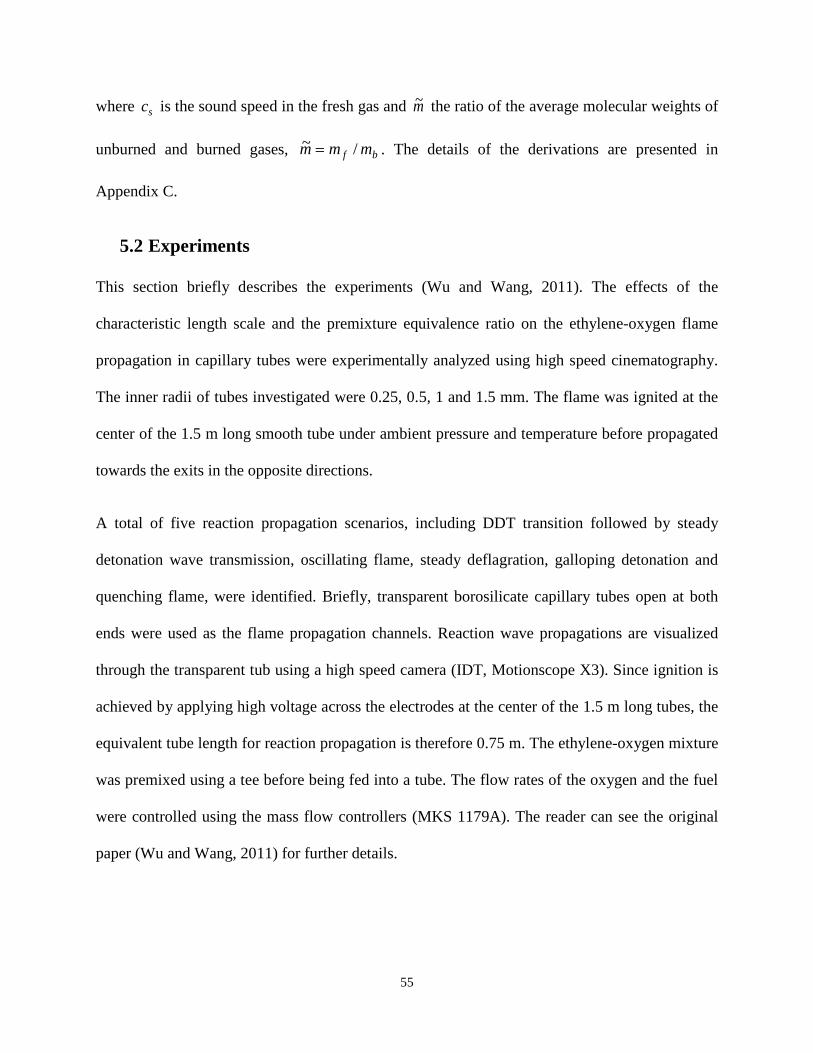
55

where sc is the sound speed in the fresh gas and m~ the ratio of the average molecular weights of

unburned and burned gases, bf mmm /~ = . The details of the derivations are presented in

Appendix C.

5.2 Experiments

This section briefly describes the experiments (Wu and Wang, 2011). The effects of the

characteristic length scale and the premixture equivalence ratio on the ethylene-oxygen flame

propagation in capillary tubes were experimentally analyzed using high speed cinematography.

The inner radii of tubes investigated were 0.25, 0.5, 1 and 1.5 mm. The flame was ignited at the

center of the 1.5 m long smooth tube under ambient pressure and temperature before propagated

towards the exits in the opposite directions.

A total of five reaction propagation scenarios, including DDT transition followed by steady

detonation wave transmission, oscillating flame, steady deflagration, galloping detonation and

quenching flame, were identified. Briefly, transparent borosilicate capillary tubes open at both

ends were used as the flame propagation channels. Reaction wave propagations are visualized

through the transparent tub using a high speed camera (IDT, Motionscope X3). Since ignition is

achieved by applying high voltage across the electrodes at the center of the 1.5 m long tubes, the

equivalent tube length for reaction propagation is therefore 0.75 m. The ethylene-oxygen mixture

was premixed using a tee before being fed into a tube. The flow rates of the oxygen and the fuel

were controlled using the mass flow controllers (MKS 1179A). The reader can see the original

paper (Wu and Wang, 2011) for further details.

56

5.3 Computational Simulations

Extensive direct numerical simulations of the hydrodynamic and combustion equations including

Arrhenius chemical kinetics and transport processes have been performed in an axisymmetric,

cylindrical geometry, the basic equations read

( ) ( ) 01=

∂∂

+∂∂

+∂∂

zr uz

urrrt

ρρρ , ( ) ( )( )

−∇+

∂∂

−=−∇⋅+∂∂

22

2

ruu

rP

ruuu

tr

rrr ζρρρ θu , (5.9)

( ) ( )( )

−∇+

∂∂

−=+∇⋅+∂∂

22

ruu

rP

ruuuu

tr

rθ

θθ

θ ζρρρ u , (5.10)

( ) ( )( ) zzz uzPuu

t2∇+

∂∂

−=∇⋅+∂∂ ζρρ u (5.11)

−−−++

∂∂

+

+

∂∂

θθγγγρρρρε ,,,22

21

21

rzrzrrrrrr rurururqurhrurrt

uu

021

,,,2 =

−−−++

∂∂

+ θθγγγρρ zzrrzzzzzz uuuquhuz

u , (5.12)

( ) ( )TREYzY

ScYu

zrYrYur

rrY

t paR

zr −−=

∂∂

−∂∂

+

∂∂

−∂∂

+∂∂ exp

Sc1

τρζρζρρ , (5.13)

( )z

ur

u zr ∂∂

+∂∂

≡∇⋅u , 2

22 1

zrr

rr ∂∂

+

∂∂

∂∂

≡∇ , (5.14)

the stress tensor ji,γ takes the form

rur

rr ∂∂

= ζγ 2, ,

−

∂∂

=r

uru

rθθ

θ ζγ , ,

∂∂

+∂∂

=zu

ru rz

zr ζγ , , zuz

zz ∂∂

= ζγ 2, , zuz

zz ∂∂

= ζγ 2, , (5.15)

and the energy diffusion vector iq is

∂∂

+∂∂

−=rYQ

rTCq P

r ScPrζ ,

∂∂

+∂∂

−=zYQ

zTCq P

z ScPrζ . (5.16)

57

5.4 Results and Discussion

In this section, new computational results are compared to the extension of the theory

(Akkerman et al., 2006) and the experimental data on premixed stoichiometric ethylene-oxygen

flames accelerating in tubes of small radii, R=0.25 and 0.5mm. Following the GasEQ and USC

Mech II results for stoichiometric ethylene-oxygen combustion, the kinematic viscosity

sm /1035.1 25−×=ν and the laminar flame speed smU f /58.3= are used, thereby making the

flame propagation Reynolds number for such tubes to be about .460~56Re = The adiabatic

exponent is 34.1/ == VP ccγ yielding the sound speed being smPcs /331/ 0 == ργ , with the

initial Mach number 0125.0/ 00 == cUM f . With the initial expansion ratio of 6.10=Θ , one

finds 34.1)//(~00 =Θ= TTm b .

It is recalled that the evolution of the flame velocity in the experiments showed humps and cusps

in the early stage of combustion, until a self-sustained state of flame acceleration is achieved. For

a meaningful comparison, one therefore had to employ the initial experimental marker related to

self-sustained flame acceleration as the initial condition for the theoretical formulation, with the

experimental flame speed at that instant assuming the role of ssΩ , and hence considerably

increasing the Mach number as compared to the initial one. Consequently, while the comparison

becomes feasible for narrow tubes, mmR )5.025.0( −= , the self-sustained flame propagation in

a wider tube, mmR )5.10.1( −= , appears outside the validity domain of the theory that assumes

weak compressibility.

58

FIG. 5.1. Evolution of the flame tip in a tube of radii R=0.25 mm (a) and 0.5mm (b)

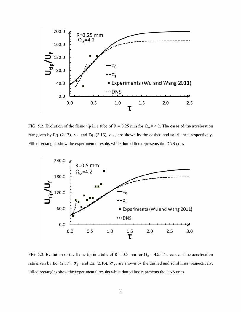
59

FIG. 5.2. Evolution of the flame tip in a tube of R = 0.25 mm for Ωss = 4.2. The cases of the acceleration

rate given by Eq. (2.17), 1σ and Eq. (2.16), 0σ , are shown by the dashed and solid lines, respectively.

Filled rectangles show the experimental results while dotted line represents the DNS ones

FIG. 5.3. Evolution of the flame tip in a tube of R = 0.5 mm for Ωss = 4.2. The cases of the acceleration

rate given by Eq. (2.17), ,1σ and Eq. (2.16), 0σ , are shown by the dashed and solid lines, respectively.

Filled rectangles show the experimental results while dotted line represents the DNS ones

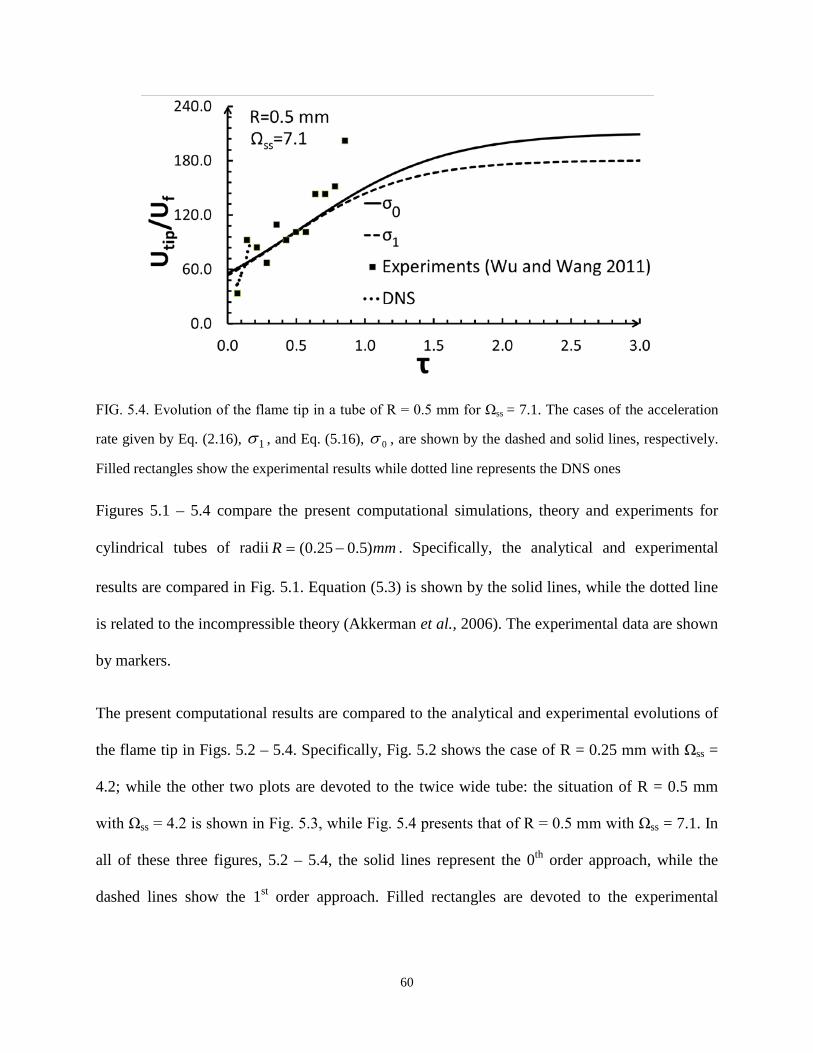
60

FIG. 5.4. Evolution of the flame tip in a tube of R = 0.5 mm for Ωss = 7.1. The cases of the acceleration

rate given by Eq. (2.16), 1σ , and Eq. (5.16), 0σ , are shown by the dashed and solid lines, respectively.

Filled rectangles show the experimental results while dotted line represents the DNS ones

Figures 5.1 – 5.4 compare the present computational simulations, theory and experiments for

cylindrical tubes of radii mmR )5.025.0( −= . Specifically, the analytical and experimental

results are compared in Fig. 5.1. Equation (5.3) is shown by the solid lines, while the dotted line

is related to the incompressible theory (Akkerman et al., 2006). The experimental data are shown

by markers.

The present computational results are compared to the analytical and experimental evolutions of

the flame tip in Figs. 5.2 – 5.4. Specifically, Fig. 5.2 shows the case of R = 0.25 mm with Ωss =

4.2; while the other two plots are devoted to the twice wide tube: the situation of R = 0.5 mm

with Ωss = 4.2 is shown in Fig. 5.3, while Fig. 5.4 presents that of R = 0.5 mm with Ωss = 7.1. In

all of these three figures, 5.2 – 5.4, the solid lines represent the 0th order approach, while the

dashed lines show the 1st order approach. Filled rectangles are devoted to the experimental

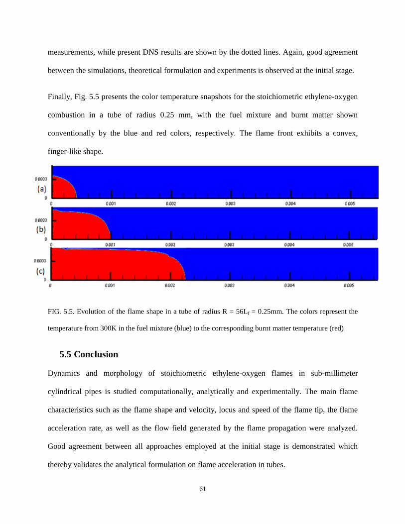
61

measurements, while present DNS results are shown by the dotted lines. Again, good agreement

between the simulations, theoretical formulation and experiments is observed at the initial stage.

Finally, Fig. 5.5 presents the color temperature snapshots for the stoichiometric ethylene-oxygen

combustion in a tube of radius 0.25 mm, with the fuel mixture and burnt matter shown

conventionally by the blue and red colors, respectively. The flame front exhibits a convex,

finger-like shape.

FIG. 5.5. Evolution of the flame shape in a tube of radius R = 56Lf = 0.25mm. The colors represent the

temperature from 300K in the fuel mixture (blue) to the corresponding burnt matter temperature (red)

5.5 Conclusion

Dynamics and morphology of stoichiometric ethylene-oxygen flames in sub-millimeter

cylindrical pipes is studied computationally, analytically and experimentally. The main flame

characteristics such as the flame shape and velocity, locus and speed of the flame tip, the flame

acceleration rate, as well as the flow field generated by the flame propagation were analyzed.

Good agreement between all approaches employed at the initial stage is demonstrated which

thereby validates the analytical formulation on flame acceleration in tubes.

62

Chapter 6: Summary

The present thesis had several objectives devoted to the comprehensive (analytical,

computational and experimental) investigation of the flame acceleration in tubes/channels due to

wall friction. A “road map” for this work was the theoretical formulation of Bychkov and co-

authors who have revealed the entire scenario of flame acceleration and detonation triggering.

One of the objectives of this thesis was to investigate the intrinsic limitations and accuracy of the

theories (Bychkov et al., 2005; Akkerman et al., 2006). This task was performed by utilizing the

Newton-Raphson and numerical discretization methods. The limitations and accuracy of the

theories were clearly underlined in the Re-Θ diagram. Another objective of the thesis was to

identify the influence of the thermal expansion and on the intrinsic accuracy of the theory as well

as on the flame propagation in general. It was clearly shown that the theory predicts the main

characteristics of the flame acceleration very well when both Θ and Re are large enough.

However, the theory quantitatively deteriorates for 86 <Θ≤ depending on Re. Eventually, the

theory breaks as soon as the expansion factor goes below 6. Finally, the last objective was to

scrutinize the dynamics and morphology of stoichiometric ethylene-oxygen flames in sub-

millimeter cylindrical pipes and bridge the gap between the experiments done by Wu and Wang

(2011) and our analytical formulation by using DNS. In this part, the main flame characteristics

such as the flame shape and velocity, the locus and speed of the flame tip, the acceleration rate,

as well as the flow field generated by the flame propagation are determined, and good agreement

between all approaches (analytical, computational and experimental) is found at the initially state

of the flame acceleration. This thereby validates the recent analytical formulations (Bychkov et

al., 2006; Akkerman et al., 2006; Bychkov et al., 2010).

63

References

V. Akkerman, V. Bychkov, A. Petchenko, L.-E. Eriksson, Combust. Flame 145 206–219 (2006).

V. Akkerman, V. Bychkov, and L. E. Eriksson, Combust.Flame 151, 452 (2007).

V. Akkerman, V. Bychkov, L. de Goey, R. Bastiaans, J. van Oijen, and L.-E. Eriksson, Phys.

Fluids 20, 055107 (2008).

V. Akkerman, C.K. Law and V. Bychkov, Phys. Rev. E 83, 026305 (2011).

V.Akkerman, C.K Law, V. Bychkov, L.E. Eriksson, Phys. Fluids 22, 053606 (2010).

N. Anderson, Eriksson, L.-E., and Davidson, L., AIAA Journal 43, p. 1899 (2005).

V. Bychkov, A. Petchenko, V. Akkerman, L.E. Eriksson, Phys. Rev. E 72, 046307 (2005).

V. Bychkov, V. Akkerman, Phys. Rev. E 73, 066305 (2006).

V. Bychkov, M.A Liberman, Physical Reorts 325, 115-237 (2000).

V. Bychkov, D. Valiev, L.-E. Eriksson,. 101 164501 (2008).

V. Bychkov, V. Akkerman, G. Fru, A. Petchenko, L.E, Eriksson, Combust. Flame 150, 263

(2007).

V. Bychkov, V. Akkerman, D. Valiev, C.K. Law, Phys. Rev. E 81, 026309 (2010).

V. Bychkov, A. Petchenko, V. Akkerman, and L.E. Eriksson, Phys. Rev. E 72, 046307 (2005).

B. Demirgok, V. Akkerman, Theory of Flame Acceleration in Tubes due to Wall Friction:

Intrinsic Limitations & Accuracy. 8th U. S. Nat. Combust. Meeting, Canyon, UT, May 19-22

(2013).

L.-E. Erikkson., Development and validation of highly modular flow solver versions in g2dflow

and g3dflow series for compressible viscous reacting flow. VAC Report: p. 9970-1162. (1995).

L.-E. Erikkson., Comp. Meth. Appl. Mech. Eng. 64, 95 (1987).

G. Roy, S. Frolov, A. Borisov, and D. Netzer, Prog. En. Combust. Sci. 30, 545 (2004).

64

K.I. Shelkin, Zh. Exp. Teor. Fiz. 10, 823 (1940).

J.E. Shepherd and J.H.S Lee, in Major Research Topics in Combustion, 439 (SpringerVerlag,

Hampton, VA) (1992).

O. Travnikov, V. Bychkov, and M. Liberman, Phys. Rev. E 61, 468 (2002).

D. Valiev, V. Akkerman, M. Kuznetsov, L.E. Eriksson, C.K. Law, V. Bychkov, Combust. Flame

160, 97 (2013).

D. Valiev, V. Bychkov, V. Akkerman, L.-E. Eriksson, M. Marklund, Phys. Lett. A 372 27-28

4850–4857 (2008).

D. Valiev, V. Bychkov, V. Akkerman, L.-E. Eriksson, Phys. Rev. E 80, 036317 (2009).

D. Valiev, V. Bychkov, V. Akkerman et al., Combust. Flame 157, 1012 (2010).

C. Wollblad, L. Davidson, L.-E. Eriksson, AIAA J. 44, 2340 (2006).

M.-H. Wu, M. Burke, S. Son, R. Yetter, Proc. Combust. Inst. 31 2429–2436 (2007).

M.-H. Wu, C.-Y. Wang, Proc. Combust. Inst. 33 2287–2293 (2011).

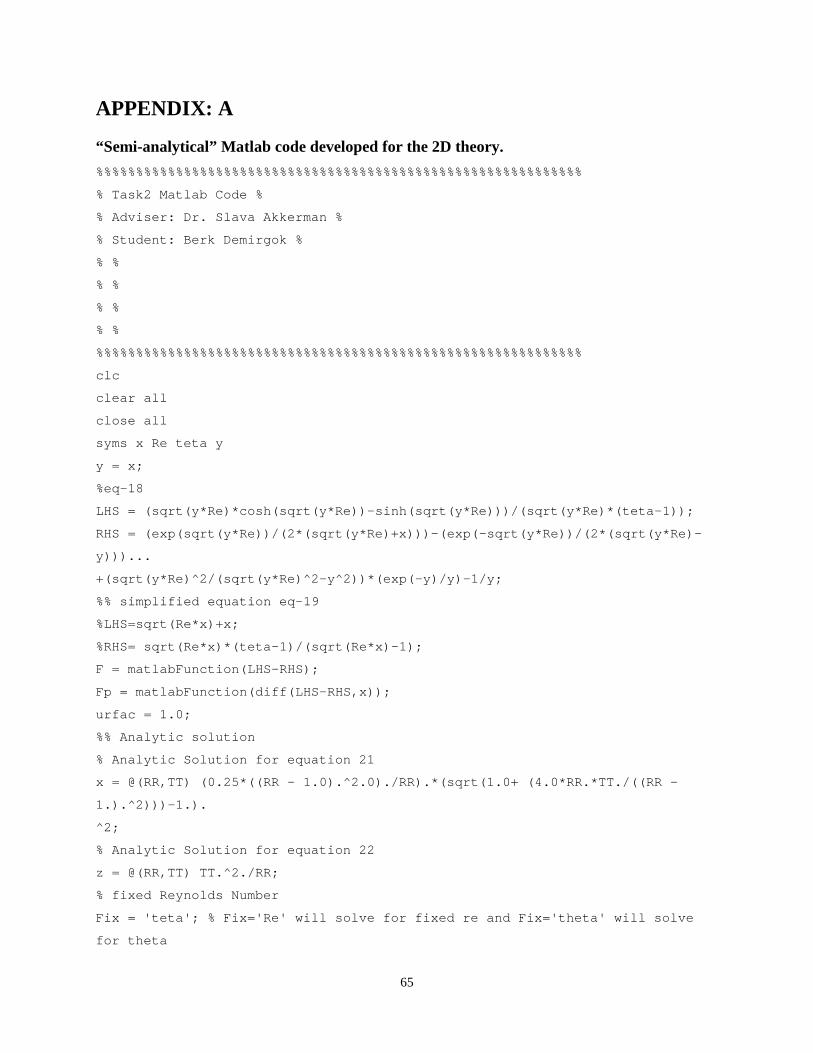
65

APPENDIX: A

“Semi-analytical” Matlab code developed for the 2D theory. %%%%%%%%%%%%%%%%%%%%%%%%%%%%%%%%%%%%%%%%%%%%%%%%%%%%%%%%%%%%%

% Task2 Matlab Code %

% Adviser: Dr. Slava Akkerman %

% Student: Berk Demirgok %

% %

% %

% %

% %

%%%%%%%%%%%%%%%%%%%%%%%%%%%%%%%%%%%%%%%%%%%%%%%%%%%%%%%%%%%%%

clc

clear all

close all

syms x Re teta y

y = x;

%eq-18

LHS = (sqrt(y*Re)*cosh(sqrt(y*Re))-sinh(sqrt(y*Re)))/(sqrt(y*Re)*(teta-1));

RHS = (exp(sqrt(y*Re))/(2*(sqrt(y*Re)+x)))-(exp(-sqrt(y*Re))/(2*(sqrt(y*Re)-

y)))...

+(sqrt(y*Re)^2/(sqrt(y*Re)^2-y^2))*(exp(-y)/y)-1/y;

%% simplified equation eq-19

%LHS=sqrt(Re*x)+x;

%RHS= sqrt(Re*x)*(teta-1)/(sqrt(Re*x)-1);

F = matlabFunction(LHS-RHS);

Fp = matlabFunction(diff(LHS-RHS,x));

urfac = 1.0;

%% Analytic solution

% Analytic Solution for equation 21

x = @(RR,TT) (0.25*((RR - 1.0).^2.0)./RR).*(sqrt(1.0+ (4.0*RR.*TT./((RR -

1.).^2)))-1.).

^2;

% Analytic Solution for equation 22

z = @(RR,TT) TT.^2./RR;

% fixed Reynolds Number

Fix = 'teta'; % Fix='Re' will solve for fixed re and Fix='theta' will solve

for theta

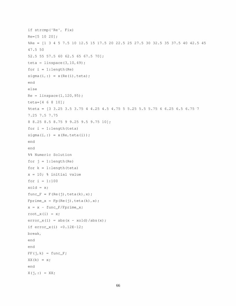
66

if strcmp('Re', Fix)

Re=[5 10 20];

%Re = [1 3 4 5 7.5 10 12.5 15 17.5 20 22.5 25 27.5 30 32.5 35 37.5 40 42.5 45

47.5 50

52.5 55 57.5 60 62.5 65 67.5 70];

teta = linspace(3,10,49);

for i = 1:length(Re)

sigma(i,:) = x(Re(i),teta);

end

else

Re = linspace(1,120,95);

teta=[4 6 8 10];

%teta = [3 3.25 3.5 3.75 4 4.25 4.5 4.75 5 5.25 5.5 5.75 6 6.25 6.5 6.75 7

7.25 7.5 7.75

8 8.25 8.5 8.75 9 9.25 9.5 9.75 10];

for i = 1:length(teta)

sigma(i,:) = x(Re,teta(i));

end

end

%% Numeric Solution

for j = 1:length(Re)

for k = 1:length(teta)

x = 10; % initial value

for i = 1:100

xold = x;

func_F = F(Re(j),teta(k),x);

Fprime_x = Fp(Re(j),teta(k),x);

x = x - func_F/Fprime_x;

root_x(i) = x;

error_x(i) = abs(x - xold)/abs(x);

if error_x(i) <0.12E-12;

break,

end

end

FF(j,k) = func_F;

XX(k) = x;

end

X(j,:) = XX;

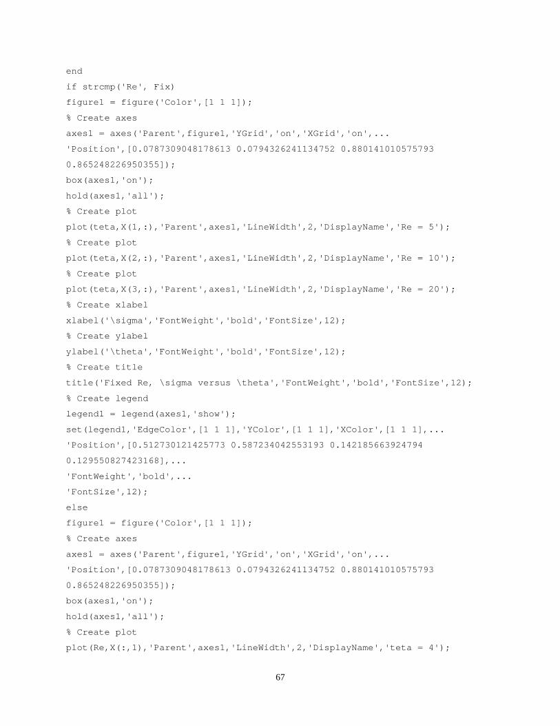
67

end

if strcmp('Re', Fix)

figure1 = figure('Color',[1 1 1]);

% Create axes

axes1 = axes('Parent',figure1,'YGrid','on','XGrid','on',...

'Position',[0.0787309048178613 0.0794326241134752 0.880141010575793

0.865248226950355]);

box(axes1,'on');

hold(axes1,'all');

% Create plot

plot(teta,X(1,:),'Parent',axes1,'LineWidth',2,'DisplayName','Re = 5');

% Create plot

plot(teta,X(2,:),'Parent',axes1,'LineWidth',2,'DisplayName','Re = 10');

% Create plot

plot(teta,X(3,:),'Parent',axes1,'LineWidth',2,'DisplayName','Re = 20');

% Create xlabel

xlabel('\sigma','FontWeight','bold','FontSize',12);

% Create ylabel

ylabel('\theta','FontWeight','bold','FontSize',12);

% Create title

title('Fixed Re, \sigma versus \theta','FontWeight','bold','FontSize',12);

% Create legend

legend1 = legend(axes1,'show');

set(legend1,'EdgeColor',[1 1 1],'YColor',[1 1 1],'XColor',[1 1 1],...

'Position',[0.512730121425773 0.587234042553193 0.142185663924794

0.129550827423168],...

'FontWeight','bold',...

'FontSize',12);

else

figure1 = figure('Color',[1 1 1]);

% Create axes

axes1 = axes('Parent',figure1,'YGrid','on','XGrid','on',...

'Position',[0.0787309048178613 0.0794326241134752 0.880141010575793

0.865248226950355]);

box(axes1,'on');

hold(axes1,'all');

% Create plot

plot(Re,X(:,1),'Parent',axes1,'LineWidth',2,'DisplayName','teta = 4');

68

% Create plot

plot(Re,X(:,2),'Parent',axes1,'LineWidth',2,'DisplayName','teta = 6');

% Create plot

plot(Re,X(:,3),'Parent',axes1,'LineWidth',2,'DisplayName','teta = 8');

% Create plot

plot(Re,X(:,4),'Parent',axes1,'LineWidth',2,'DisplayName','teta = 10');

% Create xlabel

xlabel('\sigma','FontWeight','bold','FontSize',12);

% Create ylabel

ylabel('Re','FontWeight','bold','FontSize',12);

% Create title

title('Fixed Teta, \sigma versus Re','FontWeight','bold','FontSize',12);

% Create legend

legend1 = legend(axes1,'show');

set(legend1,'EdgeColor',[1 1 1],'YColor',[1 1 1],'XColor',[1 1 1],...

'Position',[0.512730121425773 0.587234042553193 0.142185663924794

0.129550827423168],...

'FontWeight','bold',...

'FontSize',12);

end

hold on

if strcmp('Re', Fix)

plot(teta,sigma(1,:),teta,sigma(2,:),teta,sigma(3,:))

hold off

Error = 100*abs((sigma'-X')./sigma');

% plotting Errors ---------------------------------------------------------

figure1 = figure('Color',[1 1 1]);

% Create axes

axes1 = axes('Parent',figure1,'YMinorTick','on','XMinorTick','on',...

'Position',[0.109612141652614 0.117962466487936 0.851602023608769

0.807037533512064]);

% Uncomment the following line to preserve the X-limits of the axes

% xlim(axes1,[3 11]);

% Uncomment the following line to preserve the Y-limits of the axes

% ylim(axes1,[0 105]);

hold(axes1,'all');

% Create multiple lines using matrix input to plot

plot1 = plot(Error,teta,'Parent',axes1,'LineWidth',2);

69

set(plot1(1),'DisplayName','Re = 5');

set(plot1(2),'DisplayName','Re = 10');

set(plot1(3),'DisplayName','Re = 20');

% Create xlabel

xlabel('Error (%)','FontWeight','bold','FontSize',16);

% Create ylabel

ylabel('theta','FontWeight','bold','FontSize',12);

% Create legend

legend1 = legend(axes1,'show');

set(legend1,'EdgeColor',[1 1 1],'YColor',[1 1 1],'XColor',[1 1 1],...

'Position',[0.366255029937709 0.365025711279218 0.201160541586074

0.147249190938511]);

else

plot(Re,sigma(1,:),Re,sigma(2,:),Re,sigma(3,:),Re,sigma(4,:))

hold off

Error = 100*(abs((sigma'-X)./sigma'));

% plotting the error ------------------------------------------------------

figure1 = figure('Color',[1 1 1]);

% Create axes

axes1 = axes('Parent',figure1,'YMinorTick','on','XMinorTick','on',...

'Position',[0.109612141652614 0.117962466487936 0.851602023608769

0.807037533512064]);

% Uncomment the following line to preserve the X-limits of the axes

% xlim(axes1,[3 11]);

% Uncomment the following line to preserve the Y-limits of the axes

% ylim(axes1,[0 105]);

hold(axes1,'all');

% Create multiple lines using matrix input to plot

plot1 = plot(Error,Re,'Parent',axes1,'LineWidth',2);

set(plot1(1),'DisplayName','\theta = 4');

set(plot1(2),'DisplayName','\theta = 6');

set(plot1(3),'DisplayName','\theta = 8');

set(plot1(4),'DisplayName','\theta = 10');

% Create xlabel

xlabel('Error (%)','FontWeight','bold','FontSize',14);

% Create ylabel

ylabel('Re','FontWeight','bold','FontSize',12);

% Create legend

70

legend1 = legend(axes1,'show');

set(legend1,'EdgeColor',[1 1 1],'YColor',[1 1 1],'XColor',[1 1 1],...

'Position',[0.366255029937709 0.365025711279218 0.201160541586074

0.147249190938511]);

End

Semi-analytical” Matlab code developed for the axisymmetric theory.

%%%%%%%%%%%%%%%%%%%%%%%%%%%%%%%%%%%%%%%%%%%%%%%%%%%%%%%%%%%%%

% Task3 Matlab Code %

% Adviser: Dr. Slava Akkerman %

% Student: Berk Demirgok %

% %

% %

% %

% %

%%%%%%%%%%%%%%%%%%%%%%%%%%%%%%%%%%%%%%%%%%%%%%%%%%%%%%%%%%%%%

% sigma = x

clc

clear all

close all

syms RR TT

mu = (RR./2).*((1+(8.*(TT-1))./(RR)).^0.5-1);

an = (RR./4.0).*((1.0+(8.0.*(TT-1))./(RR)).^0.5-1).^2.0;

ann = (RR./4).*((1+((8.*(TT-1))./RR).*(1+(1./mu)+(1./(2.*(mu+an))))).^(0.5)-

1).^2.0;

anF = matlabFunction(ann); % anF = F(RR, TT)

muf =matlabFunction(mu);

syms x y Re nu teta

% Analytic Solution for equation 21

% mu= @(RR,TT) (RR/2.0).*(sqrt(1.0+(8.0*(TT-1))./(RR))-1);

an = @(RR,TT) (RR./4.0).*((1.0+(8.0.*(TT-1))./(RR)).^0.5-1).^2.0;

%ann = @(RR,TT) (RR/4.0).*(sqrt(1.0+((8.0*(TT-

1))./(RR)).*(1.0+1.0/((RR/2.0).*(sqrt(1.0+

(8.0*(TT-1))./(RR))-1))+1.0/(2.0*(((RR/2.0).*(sqrt(1.0+(8.0*(TT-1))./(RR))-

1))+((RR/4.

0).*(sqrt(1.0+(8.0*(TT-1))./(RR))-1).^2.0)))))-1).^2.0;

71

%ann = @(RR,TT,mu,an) (RR/4.0).*(1+sqrt(1.0+((8.0*(TT-

1))./(RR))*(1.0+(1.0/(mu))+(1/(2*

(mu+an))))-1)).^2.0;

arg = sqrt(x*Re);

func = besseli(0,arg*y)*exp(x*y);

% F --> f(Re,x,y)

F = matlabFunction(func);

% Integration: KSI(nu): Using numerical discretization to calculate

% integration symbolically

n = 41; % # of grids in discrete domain

FF = 0;

h = nu/(n-1);

for i = 2:n-1

tt = h*(i-1);

FF = FF + F(Re,x,tt);

end

KSI_n = 0.5*h*(F(Re,x,0) + F(Re,x,nu))+h*FF;

eKSI = KSI_n*exp(-x*nu);

FeKSI = matlabFunction(eKSI); % FeKSI--> f(Re,nu,x)

% KSI(1)*exp(-sig)

exKSI_1 = FeKSI(Re,1,x);

% Symbolic Integration using numerical discretization

% int, KSI(n)exp(-sig*nu)dnu (0,1)

Ff = 0;

h = 1/(n-1);

for i = 2:n-1

tt = h*(i-1);

Ff = Ff + FeKSI(Re,tt,x);

end

intKSI = 0.5*h*(FeKSI(Re,0,x) + FeKSI(Re,1,x))+h*Ff;

LHS = (besseli(0,arg)-2*arg^(-1)*besseli(1,arg))/(2*(teta-1));

RHS = (((x+1)*exp(-x)-1)/x^2)+exKSI_1-intKSI;

% General nonlinear Equation : Fsys = f(Re,teta,x)

Fsys = matlabFunction(LHS-RHS);

Fprime = matlabFunction(diff((LHS-RHS),x)); % Fprime = f(Re,teta,x)

% fixed Reynolds Number

Fix = 'Re'; % Fix='Re' will solve for fixed re and Fix='theta' will solve for

theta

72

if strcmp('Re', Fix)

Re = [40 60 80];

teta = linspace(2,6,50);

for i = 1:length(Re)

%mu_(i,:) = mu(Re(i),teta);

sigma(i,:) = anF(Re(i),teta);

sigmaa(i,:)=an(Re(i),teta);

end

else

Re = linspace(1,200,100);

teta = [4 6 8 10 12];

for i = 1:length(teta)

% mu_(i,:) = mu(Re,teta(i));

sigma(i,:) = anF(Re,teta(i));

sigmaa(i,:)=an(Re,teta(i));

end

end

for j = 1:length(Re)

for k = 1:length(teta)

x = 7; % initial value

for i = 1:100

xold = x;

func_F = Fsys(Re(j),teta(k),x);

Fprime_x = Fprime(Re(j),teta(k),x);

x = x - func_F/Fprime_x;

root_x(i) = x;

error_x(i) = abs(x - xold);

if error_x(i) <0.12E-6;

break,

end

end

FF(j,k) = func_F;

XX(k) = x;

end

X(j,:) = XX;

end

% %%%%%%%%%%%%%%%%%%%%%%%%%%%%%%%%%%%%%%%%%%%%%%%%%%%%%%%%%%%%%%%%%%%%%%%%%%

%fixed theta plots

73

% figure

% plot(Re,sigma(1,:),'r')

% hold on

% plot(Re,sigma(2,:),'b')

% hold on

% plot(Re,sigma(3,:),'g')

% hold on

% plot(Re,X(:,1),'r.')

% hold on

% plot(Re,X(:,2),'b.')

% hold on

% plot(Re,X(:,3),'g.')

% hold on

% xlabel('\Re')

% ylabel('\Theta')

%

% plot(Re,sigmaa(1,:),'r--')

% hold on

% plot(Re,sigmaa(2,:),'b--')

% hold on

% plot(Re,sigmaa(3,:),'g--')

%

% Error = 100*(abs((sigma'-X)./sigma'));

% figure

% plot(Re,Error)

% xlabel('Re')

% ylabel('Error (%)')

% figure

% %contour(teta,Re,Error,5)

% contour(teta,Re,Error,'ShowText','on','LevelList',[ 5 10 15 30 50 ]);

% xlabel('\Theta')

% ylabel('\Re')

% %

%%%%%%%%%%%%%%%%%%%%%%%%%%%%%%%%%%%%%%%%%%%%%%%%%%%%%%%%%%%%%%%%%%%%%%%%%%

% %fixed Re plots

figure

plot(teta,sigma(1,:),'r')

hold on

74

plot(teta,sigma(2,:),'b')

hold on

plot(teta,sigma(3,:),'g')

hold on

plot(teta,X(1,:),'r.')

hold on

plot(teta,X(2,:),'b.')

hold on

plot(teta,X(3,:),'g.')

hold on

plot(teta,sigmaa(1,:),'r--')

hold on

plot(teta,sigmaa(2,:),'b--')

hold on

plot(teta,sigmaa(3,:),'g--')

hold on

xlabel('\Theta')

ylabel('\sigma')

Error = 100*(abs((sigma-X)./sigma));

figure

plot(teta,Error)

xlabel('\Theta')

ylabel('Error %')

figure

%contour(teta,Re,Error,5)

contour(teta,Re,Error,'ShowText','on','LevelList',[1 3 5 10 15 25 35 50]);

xlabel('\Theta')

ylabel('\Re')

%%%%%%%%%%%%%%%%%%%%%%%%%%%%%%%%%%%%%%%%%%%%%%%%%%%%%%%%%%%%%%%%%%%%%%%%%%

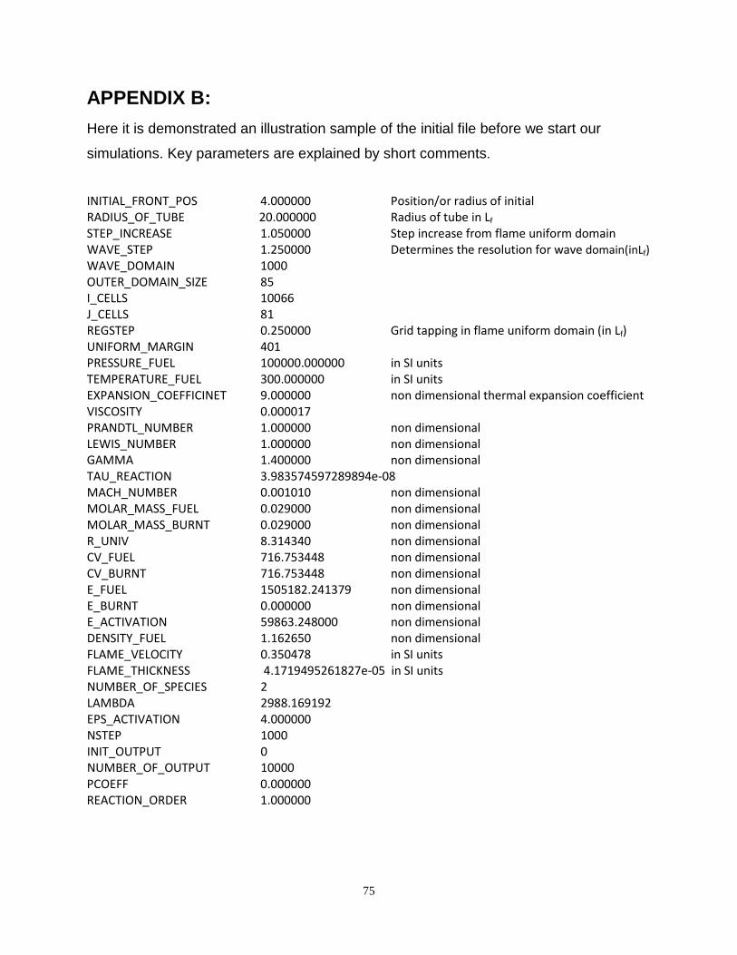
75

APPENDIX B: Here it is demonstrated an illustration sample of the initial file before we start our

simulations. Key parameters are explained by short comments.

INITIAL_FRONT_POS 4.000000 Position/or radius of initial RADIUS_OF_TUBE 20.000000 Radius of tube in Lf STEP_INCREASE 1.050000 Step increase from flame uniform domain WAVE_STEP 1.250000 Determines the resolution for wave domain(inLf) WAVE_DOMAIN 1000 OUTER_DOMAIN_SIZE 85 I_CELLS 10066 J_CELLS 81 REGSTEP 0.250000 Grid tapping in flame uniform domain (in Lf) UNIFORM_MARGIN 401 PRESSURE_FUEL 100000.000000 in SI units TEMPERATURE_FUEL 300.000000 in SI units EXPANSION_COEFFICINET 9.000000 non dimensional thermal expansion coefficient VISCOSITY 0.000017 PRANDTL_NUMBER 1.000000 non dimensional LEWIS_NUMBER 1.000000 non dimensional GAMMA 1.400000 non dimensional TAU_REACTION 3.983574597289894e-08 MACH_NUMBER 0.001010 non dimensional MOLAR_MASS_FUEL 0.029000 non dimensional MOLAR_MASS_BURNT 0.029000 non dimensional R_UNIV 8.314340 non dimensional CV_FUEL 716.753448 non dimensional CV_BURNT 716.753448 non dimensional E_FUEL 1505182.241379 non dimensional E_BURNT 0.000000 non dimensional E_ACTIVATION 59863.248000 non dimensional DENSITY_FUEL 1.162650 non dimensional FLAME_VELOCITY 0.350478 in SI units FLAME_THICKNESS 4.1719495261827e-05 in SI units NUMBER_OF_SPECIES 2 LAMBDA 2988.169192 EPS_ACTIVATION 4.000000 NSTEP 1000 INIT_OUTPUT 0 NUMBER_OF_OUTPUT 10000 PCOEFF 0.000000 REACTION_ORDER 1.000000

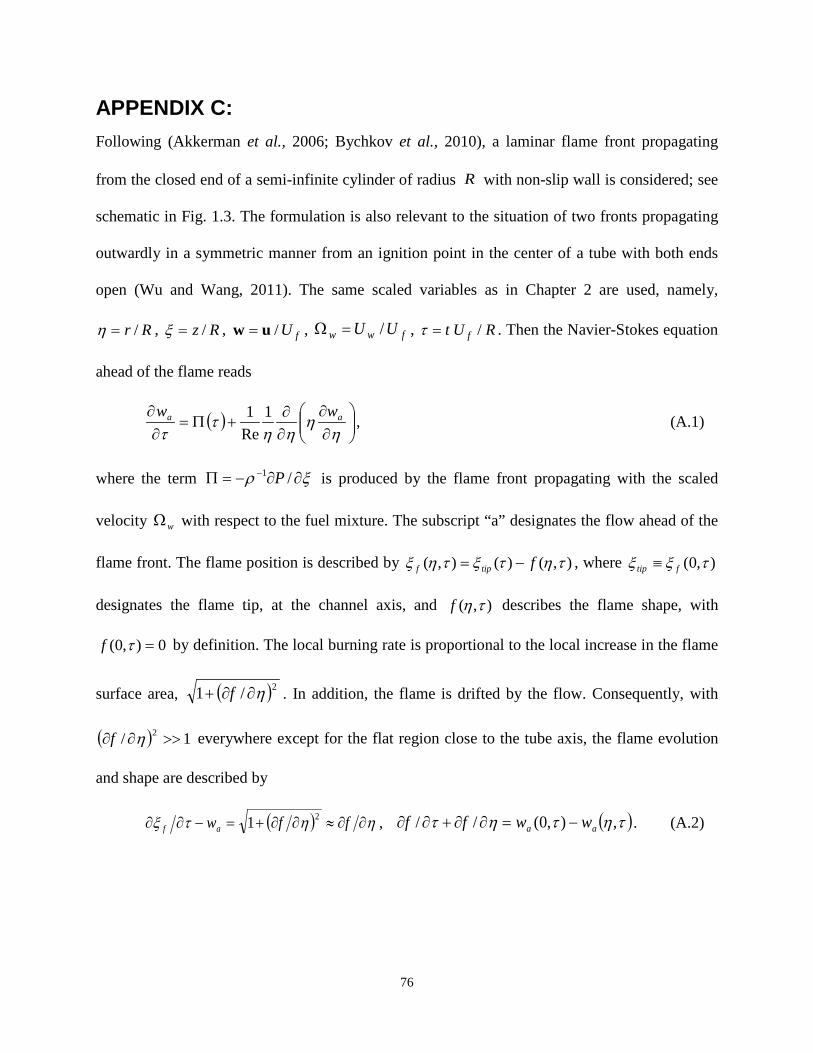
76

APPENDIX C: Following (Akkerman et al., 2006; Bychkov et al., 2010), a laminar flame front propagating

from the closed end of a semi-infinite cylinder of radius R with non-slip wall is considered; see

schematic in Fig. 1.3. The formulation is also relevant to the situation of two fronts propagating

outwardly in a symmetric manner from an ignition point in the center of a tube with both ends

open (Wu and Wang, 2011). The same scaled variables as in Chapter 2 are used, namely,

Rr /=η , Rz /=ξ , fU/uw = , fww UU /=Ω , RUt f /=τ . Then the Navier-Stokes equation

ahead of the flame reads

( )

∂∂

∂∂

+Π=∂

∂η

ηηη

ττ

aa ww 1Re1 , (A.1)

where the term ξρ ∂∂−=Π − /1 P is produced by the flame front propagating with the scaled

velocity wΩ with respect to the fuel mixture. The subscript “a” designates the flow ahead of the

flame front. The flame position is described by ),()(),( τητξτηξ ftipf −= , where ),0( τξξ ftip ≡

designates the flame tip, at the channel axis, and ),( τηf describes the flame shape, with

0),0( =τf by definition. The local burning rate is proportional to the local increase in the flame

surface area, ( )2/1 η∂∂+ f . In addition, the flame is drifted by the flow. Consequently, with

( ) 1/ 2 >>∂∂ ηf everywhere except for the flat region close to the tube axis, the flame evolution

and shape are described by

( ) ηητξ ∂∂≈∂∂+=−∂∂ ffwaf21 , ( )τητητ ,),0(// aa wwff −=∂∂+∂∂ . (A.2)

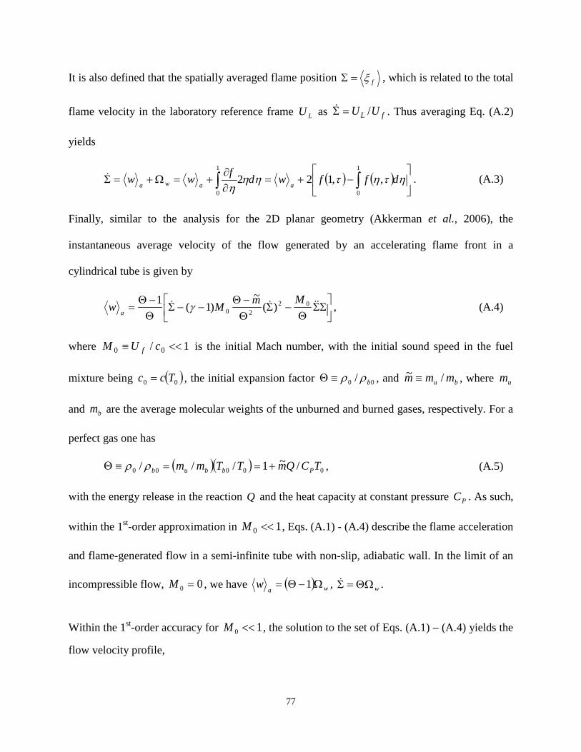
77

It is also defined that the spatially averaged flame position fξ=Σ , which is related to the total

flame velocity in the laboratory reference frame LU as fL UU /=Σ . Thus averaging Eq. (A.2)

yields

( ) ( )

−+=

∂∂

+=Ω+=Σ ∫∫ ητητηηη

dffwdfwwaawa

1

0

1

0

,,122 . (A.3)

Finally, similar to the analysis for the 2D planar geometry (Akkerman et al., 2006), the

instantaneous average velocity of the flow generated by an accelerating flame front in a

cylindrical tube is given by

ΣΣ

Θ−Σ

Θ−Θ

−−ΣΘ−Θ

= 0220 )(~

)1(1 MmMwa

γ , (A.4)

where 1/ 00 <<≡ cUM f is the initial Mach number, with the initial sound speed in the fuel

mixture being ( )00 Tcc = , the initial expansion factor 00 / bρρ≡Θ , and bu mmm /~ ≡ , where um

and bm are the average molecular weights of the unburned and burned gases, respectively. For a

perfect gas one has

( )( ) 00000 /~1/// TCQmTTmm Pbbub +==≡Θ ρρ , (A.5)

with the energy release in the reaction Q and the heat capacity at constant pressure PC . As such,

within the 1st-order approximation in 10 <<M , Eqs. (A.1) - (A.4) describe the flame acceleration

and flame-generated flow in a semi-infinite tube with non-slip, adiabatic wall. In the limit of an

incompressible flow, 00 =M , we have ( ) waw Ω−Θ= 1 , wΘΩ=Σ .

Within the 1st-order accuracy for 10 <<M , the solution to the set of Eqs. (A.1) – (A.4) yields the

flow velocity profile,

78

( ) ( ) ( )[ ] ( )−

−−

−Ω−Θ≈ στ

ηηµ

µµτη exp1exp1

21, ssaw

( ) ( )[ ] ( )στη

ηµµ

µ 2exp12exp12

1 220

−−

−Ω−Θ ssAM , (A.6)

with the average velocity

( ) ( ) ( ) ( )στστ 2exp1exp1 220 ssssaAMw Ω−Θ−Ω−Θ= . (A.7)

The flame shape is described as

( ) ( )[ ]( )

( ) ( )[ ] ( )−

−−−−+

−−

Ω−Θ≈ στσηµσπµη

ησµηµ

µµτη expexp1exp

21exp2

)1(, ssf

( )[ ]( ) ( ) ( )[ ] ( )στσηµπµη

σησµηµ

µµ

2exp2exp12exp2

122

12exp2

)1( 22

0

−−−−+

−−

Ω−Θ ssAM , (A.8)

such that the total burning rate is given by

( ) ( ) ( ) ( ) ( )στστητητ 2exp1exp,,12 220

1

0

BAMdff ssssw Ω−Θ−Ω=

−=Ω ∫ , (A.9)

where

( )[ ] 12/

−+= µσB , ( )( )[ ]

−

−ΘΘ+−Θ−= BmA

11~1γ . (A.10)

Consequently, the total flame speed with respect to the laboratory reference frame read

( ) ( ) ( ) ( )στστ 2exp11exp 220 BAMw sssswa +Ω−Θ−ΘΩ=Ω+=Σ , (A.11)

with the average flame position,

( ) ( ) ( ) ( )στσ

στσ

2exp12

1exp 22

0 BAM ssss +Ω−Θ

−ΩΘ

=Σ , (A.12)

and its acceleration,

( ) ( ) ( ) ( )στσστσ 2exp112exp 220 BAM ssss +Ω−Θ−ΩΘ=Σ . (A.13)

Then the flame tip position is given by

79

( ) ( ) ( )στµσ

στµσ

ξ 2exp22

11exp1 220

+

+Ω−Θ−Ω

+

Θ=+Σ=

BBAMf sssstip , (A.14)

and the flame tip velocity in the laboratory reference frame

( )−Ω

+Θ=+Σ=≡ στ

µσξ expss

L

tiptip f

SU

( ) ( )στµσ 2exp2111 22

0

++Ω−Θ BAM ss . (A.15)

In the 0th order approximation in 0M , Eqs. (A.6) – (A.15) reproduce the incompressible theory

of flame acceleration in cylindrical tubes (Akkerman et al., 2006), while the 1st order corrections

elucidate the moderation of the acceleration due to compressibility. It is also noted that Eqs.

(A.7), (A.9) – (A.15) agree with the respective formulas obtained in the 2D geometry (Bychkov

et al., 2010). However, even in terms of µ and σ , the factor B , Eq. (A.8), is twice the

respective 2D factor (Bychkov et al., 2010). Furthermore, in the axisymmetric case, the factor µ

is about twice that of the 2D case for the same Re. Consequently, the axisymmetric acceleration

exponent σ is about 4 times larger than the planar one, yielding considerably stronger flame

acceleration, as well as the stronger relative effect of the moderation, in the cylindrical,

axisymmetric geometry.

The moderating flame acceleration can be further demonstrated in the form of a differential

equation for the average flame position. In the 0th order approximation of 0M , the accelerating

flame dynamics is determined by the differential equation

Σ=Σ σ , (A.16)

which can be extended in the 1st order approximation as

( )Σ−Σ=Σ 11 Cσ , (A.17)

80

with ( ) ( )BAMC +Θ−= − 1121

01 . Integration of Eq. (A.17) with the initial condition

( ) ( )BAM ssss +Ω−Θ−ΘΩ=Σ 1)1(0 220

, (A.18)

yields the average flame front velocity in the laboratory frame and the average flame position,

)exp(1

)exp(

10 στστ

ss

ss

CM ΘΩ+ΘΩ

=Σ , ( )[ ]στσ

exp1ln110

10ssCM

CMΩΘ+=Σ . (A.19)

The total burning rate and the flame tip evolution can be estimated in the similar manner. For the

burning rate, the 0th order relation, ww Ω=Ω σ , extends to

( )www CΩ−Ω=Ω~1σ , (A.20)

with ( ) ABMC 20 1~

−Θ= , initial condition ( ) BAM ssssw22

0 1)0( Ω−Θ−Ω=Ω , and the solution

)exp(~1

)exp(στ

στ

ss

ssw CΩ+

Ω=Ω . (A.21)

Similarly, the evolution of the flame tip is described by

( )tiptiptip C ξξσξ 21−= , (A.22)

( )

( ) )exp(/1)exp(/

2 στµσστµσ

ξss

sstip C Ω+Θ+

Ω+Θ= , (A.23)

( ) ( )[ ]στµσσ

ξ exp/1ln12

2sstip C

CΩ+Θ+= , (A.24)

where

( )( )

2

02021

221

/1

Θ−Θ

≈

+

+

+Θ

−Θ= AMBBAMC

µσµσ. (A.25)

Here we account for the effect of compressibility in the 1st order approximation for the initial

Mach number related to flame propagation, 1/ 00 <<≡ cUM f . In order to describe a

compression wave, we shall neglect the multi-dimensional flame structure approximating the

flame front as a one-dimensional flat discontinuity surface in the locus )(tΣ=Σ . In the limit of

81

weak compression, the isentropic approximation may be adopted. Then, the scaled density

0/~ ρρρ = , pressure 0/~ PPp = and temperature 0/~ TTT = just ahead of the flame are given by :

aaa wMwM 0

12

0 12

11~ +≈

−

+=−γγρ , (A.26)

aaa wMwMp 0

12

0 12

11~ γγ γγ

+≈

−

+=−

, (A.27)

( )aaa wMwMT 0

2

0 112

11~ −+≈

−

+= γγ , (A.28)

Matching conditions at the flame front take the form

( ) ( )bfbfaa ww −Σ=−Σ ρρ ~~ , (A.29)

( ) ( )220

220

~~~~bfbfbfaaa wMpwMp −Σ+=−Σ+ ργργ , (A.30)

( ) ( )220

220 2

1~2

11~bfbfaa wMTwMT −Σ

−+=−Σ

−+−+ γγε , (A.31)

where the index “bf” denotes the burnt matter just behind the flame front and ε stands for the

initial temperature jump across the front, with m~/Θ=ε in the perfect gas model, where m~ is

the ratio of the average molecular weights of unburned and burned gases, bu mmm /~ = . In the 1st

order approximation of 0M , Eqs. (A.30), (A.31) and the perfect gas law yield

abf pp ~~ = , 1~~ −+= εabf TT , θρρ abf~~ = , (A.32)

with the instantanoues expansion factor accounting for compressibility being

aabf TmTTm /)1(1~~/~~ −+=≡ εθ . (A.33)

Obviously, Θ=θ when compression is negligible, 00 →a

wM . But, as soon as the flame

accelerates, aT~ increases and θ reduces, thereby moderating the flame acceleration. Let us next

consider the flow in the burnt gas. From the continuity equation

82

0)~(~

=∂∂

+∂∂

bbb wρ

ξτρ , (A.34)

and the condition of adiabatic compression, γρ∝p , we find

τγτρ

ρξ dpd

pddw b

b

b

b

b~

~1~

~1

−=−=∂∂

, (A.35)

where the substantial derivative is taken for a particular gas parcel. For the same 1D model, we

have one more equation for pressure, namely

ξρξτ ∂

∂−=

∂∂

+∂

∂ b

b

bb

b pww

wM

~~12

0 . (A.35)

Neglecting the second order term of 0M in Eq. (A.35), we obtain uniform pressure distribution

in the burnt gas, so pressure is a function of time only, )(~)(~~ ττ abfb ppp == . Then

ξτγ dpd

pw a

ab

~~1

−= , Σ−=τγ dpd

pw a

abf

~~1 . (A.36)

Finally, substituting Eqs. (A.27), (A.28), (A.32) and (A.35) into Eq. (A.29), within the 1st order

approximation of 0M , we find

( ) Σ+

+Σ=−Σ

−+

τγε

dwd

wMM

wTm

a

aa

a 0

0

1~11~

1 , (A.37)

with the final result

Σ

−

−+

Θ−Σ

−

Θ−

−Θ−Θ

≈τ

γε

εγε

εdwd

wMM

wMw aaaa 0

00 )1(11)1(11

ΣΣ

Θ−Σ

Θ−Θ

−−ΣΘ−Θ

≈ 0220 )(~

)1(1 MmMγ . (A.38)