The Moody’s CreditCycle Approach to Loan Loss Modeling Introduction

Recently, Moody’s Analytics purchased, from a liquidator, data describing the characteristics and performance of the subprime mortgages originated by a large, now defunct, player in the industry. The company in question, which we will refer to as Company X, went out of business in early 2007 after trading for a number of years and after building a sizable book that stretched from coast to coast. The origination data are of generally high quality and would mimic the data sets maintained by lenders of similar size who are engaged in the consumer credit arena more broadly.

ANALYSIS

Prepared by

Cristian deRitiscristian.deritis@moodys.comSenior Director

Tony Hughestony.hughes@moodys.comManaging Director

Contact Us

Email help@economy.com

U.S./Canada +1.866.275.3266

EMEA +44.20.7772.5454 (London) +420.224.222.929 (Prague)

Asia/Pacific +852.3551.3077

All Others +1.610.235.5299

Web www.economy.com www.moodysanalytics.com

MOODY’S ANALYTICS

1 July 2014

The Moody’s CreditCycle Approach to Loan Loss Modeling By CRISTIAN DERITIS AND TONy HuGHES

Recently, Moody’s Analytics purchased, from a liquidator, data describing the characteristics and performance of the subprime mortgages originated by a large, now defunct, player in the industry. The company in question, which we will refer to as Company X, went out of business in early 2007

after trading for a number of years and after building a sizable book that stretched from coast to coast. The origination data are of generally high quality and would mimic the data sets maintained by lenders of similar size who are engaged in the consumer credit arena more broadly.

The data should be of considerable interest in the present environment. By better understanding the risk manage-ment practices and origination decisions made by the company through its his-tory, we can start to paint a picture of the forces that led to the company’s demise. Given that subprime mortgage failures are at the epicenter of the current economic malaise, obtaining a deeper perspective into why Company X failed will help il-luminate the triggers of the recession. Surviving lenders in the mortgage sector as well as those in other areas such as credit cards and autos should seek to learn from the mistakes made by the managers of the company, lest they repeat them. Learning how Company X’s risk managers could have averted disaster may save oth-ers from suffering a similar fate. If these lessons are all fully digested, there is no reason why the industry cannot emerge in stronger condition despite the depth of the problems it has experienced.

The data are also useful for conducting research more generally on credit modeling methodologies. For example, the tradition-al approach to loss forecasting employed in the industry involves aggregating the

output from loan level scoring models to derive forward estimates of delinquency rates. Roll rate models, again typically derived at the loan level, then carry the short-term delinquency rates through to defaults, which are then used to assess the bottom line. Moody’s Analytics, in contrast, has taken a different tack in analyzing this problem, arguing instead for an aggregate, vintage-based approach to loss forecast-ing. This is the method embodied in the recently released product called Moody’s CreditCycle. Moody’s Analytics has argued in a series of recent articles, based on fun-damental principles of forecasting, that the MCC methodology should consistently outperform loan level approaches in terms of forecast, and hence stress test, accuracy. This superiority has previously been dem-onstrated by using industry level data, but since MCC is designed to be applied to the performance of specific portfolios, having access to the data on Company X’s perfor-mance allows Moody’s Analytics to put the methodology to the test in a completely realistic case study.

This article describes, in some detail, using both loan level models and the MCC meth-odology, the anatomy of Company X’s delin-

quency rate performance. In so doing, the key findings from each approach are highlighted in terms of what they tell us about the company’s clientele and their management decision-making processes. A byproduct of the analysis is a comparison of the predicted outcomes from both approaches through the early years of the subprime meltdown. The final section discusses the problem of calibra-tion of loan level models using aggregate level forecasts as the basis for the calibration. By engaging in such an exercise, users will be able to derive scoring models that are consis-tent with aggregate level portfolio forecasts and related stress tests.

DataData for this exercise were obtained from

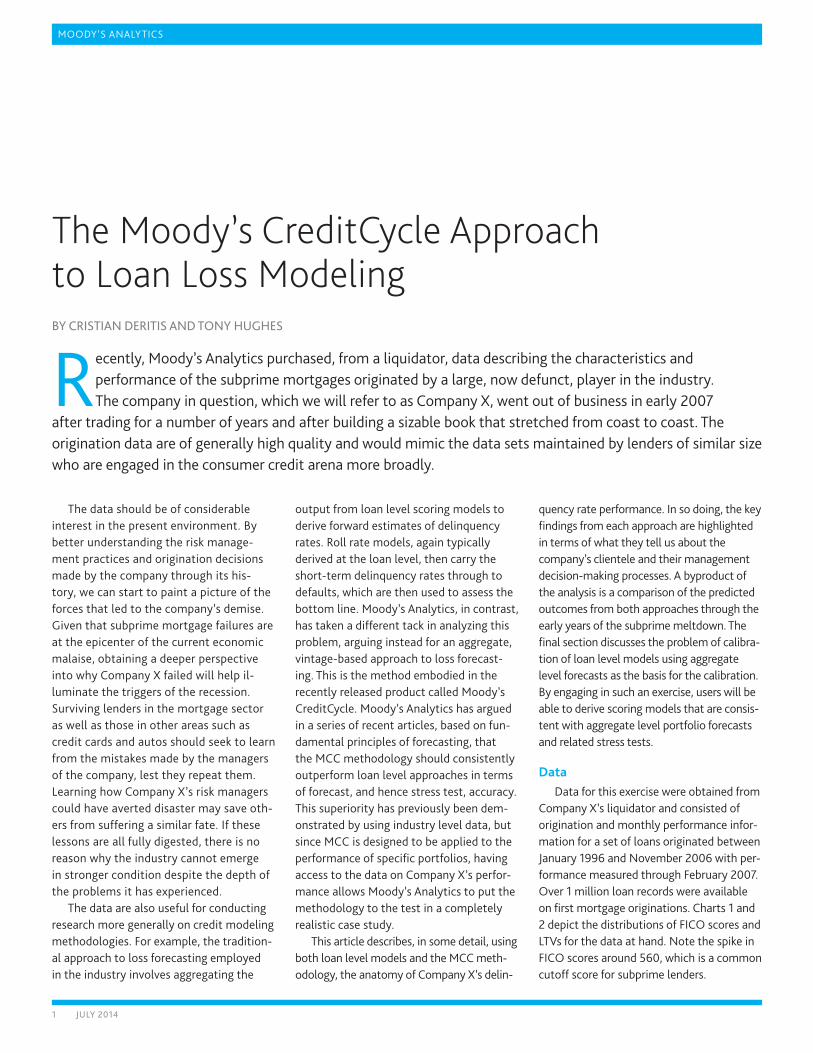
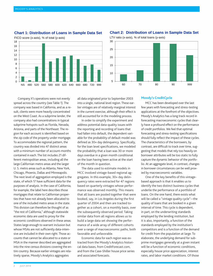
Company X’s liquidator and consisted of origination and monthly performance infor-mation for a set of loans originated between January 1996 and November 2006 with per-formance measured through February 2007. Over 1 million loan records were available on first mortgage originations. Charts 1 and 2 depict the distributions of FICO scores and LTVs for the data at hand. Note the spike in FICO scores around 560, which is a common cutoff score for subprime lenders.

MOODY’S ANALYTICS

2 July 2014

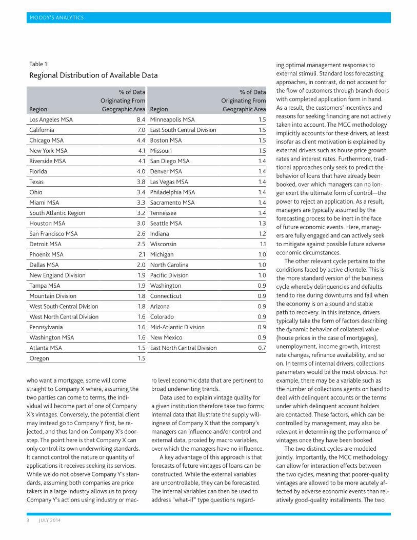
Company X’s operations were not evenly spread across the country (see Table 1). The company was based in California, and as a re-sult, clients were more heavily concentrated on the West Coast. As a subprime lender, the company also had concentrations in typical subprime hotspots such as Florida, Nevada, Arizona, and parts of the Northeast. The re-gion for each account is identified based on the zip code of the property under mortgage. To accommodate the regional pattern, the country was divided into 47 distinct areas with a minimum number of account-months contained in each. The list includes 21 dif-ferent metropolitan areas, including all the large Californian metro areas and the larger U. S. metro areas such as Atlanta, New York, Chicago, Phoenix, Dallas and Minneapolis. The next level of aggregation employed is the state, of which 17 have sufficient data for the purposes of analysis. In the case of California, for example, the label here describes those mortgages that relate to Californian proper-ties that have not already been allocated to one of the included metro areas in the state. This division can therefore be thought of as “the rest of California,” although statewide economic data are used to proxy for the economic conditions observed in these areas. States large enough to warrant inclusion but whose MSAs are not sufficiently data-inten-sive are included in their own right. Those ac-counts that cannot be allocated to a state or MSA in the manner described are aggregated into the nine census divisions covering the en-tire country. Because earlier vintages are rela-tively sparse, Moody’s Analytics aggregates

all data originated prior to September 2003 into a single, national level region. These ear-lier vintages are of relatively marginal interest in the current exercise, although their effect is still accounted for in the modeling process.

In order to simplify the experiment and address potential data-quality issues with the reporting and recording of loans that had fallen into default, the dependent vari-able for the probability of default model was defined as 30+ day delinquency. Specifically, for the loan level specifications, we modeled the probability that a loan was 30 or more days overdue in a given month conditional on the loan having been active at the start of the month in question.

The data used to estimate models in MCC involved vintage-based regional ag-gregates. In this example, 30+ day delin-quency rates were extracted for 47 regions based on quarterly vintages whose perfor-mance was observed monthly. This means that all loans are pooled together that were booked, say, in Los Angeles during the first quarter of 2004 and then are tracked to-gether as a cohort, on a monthly basis, over the subsequently observed period. Taking similar data from all regions allows us to build a large data set showing the perfor-mance of a wide array of different cohorts over a range of macroeconomic paths, both favorable and unfavorable.

Economic data for each region was ex-tracted from the Moody’s Analytics histori-cal data bases, from CreditForecast.com, and from the Case-Shiller house price series and associated forecasts.

Moody’s CreditCycleMCC has been developed over the last

few years with forecasting and stress-testing applications at the forefront of the objectives. Moody’s Analytics has a long track record in forecasting macroeconomic cycles that clear-ly have a profound effect on the performance of credit portfolios. We feel that optimal forecasting and stress-testing specifications should fully reflect the impact of these cycles. The characteristics of the borrowers, by contrast, are difficult to track over time, sug-gesting that models that rely too heavily on borrower attributes will be too static to fully capture the dynamic behavior of the portfo-lio. At an aggregate level, in contrast, changes in borrower circumstances can be well prox-ied by macroeconomic variables.

One of the key benefits of this vintage-based approach is that it enables us to identify the two distinct business cycles that underlie the performance of a portfolio of loans. On the one hand, there exists what will be called a “vintage quality cycle”—the quality of loans that are booked in a given interval of time. This cycle is dependent, in part, on the underwriting standards employed by the lending institution, but it is also, importantly, a function of the standards employed by the institution’s competitors and is a function of the demand for credit from the population at large. To elaborate, the underlying demand for sub-prime mortgages generally at a given instant will be a function of economic conditions, especially house price appreciation, interest rates, and labor market conditions. Of those

11

0

2

4

6

8

10

12

14

16

18

NS 480 520 560 580 600 620 640 660 680 720 999

Chart 1: Distribution of Loans in Sample Data SetFICO score (x-axis), % of total (y-axis)

22

5

10

15

20

25

30

60 70 80 90 999

Chart 2: Distribution of Loans in Sample Data SetLTV ratio (x-axis), % of total loans (y-axis)

MOODY’S ANALYTICS

3 July 2014

who want a mortgage, some will come straight to Company X where, assuming the two parties can come to terms, the indi-vidual will become part of one of Company X’s vintages. Conversely, the potential client may instead go to Company Y first, be re-jected, and thus land on Company X’s door-step. The point here is that Company X can only control its own underwriting standards. It cannot control the nature or quantity of applications it receives seeking its services. While we do not observe Company Y’s stan-dards, assuming both companies are price takers in a large industry allows us to proxy Company Y’s actions using industry or mac-

ro level economic data that are pertinent to broad underwriting trends.

Data used to explain vintage quality for a given institution therefore take two forms: internal data that illustrate the supply will-ingness of Company X that the company’s managers can influence and/or control and external data, proxied by macro variables, over which the managers have no influence.

A key advantage of this approach is that forecasts of future vintages of loans can be constructed. While the external variables are uncontrollable, they can be forecasted. The internal variables can then be used to address “what-if” type questions regard-

ing optimal management responses to external stimuli. Standard loss forecasting approaches, in contrast, do not account for the flow of customers through branch doors with completed application form in hand. As a result, the customers’ incentives and reasons for seeking financing are not actively taken into account. The MCC methodology implicitly accounts for these drivers, at least insofar as client motivation is explained by external drivers such as house price growth rates and interest rates. Furthermore, tradi-tional approaches only seek to predict the behavior of loans that have already been booked, over which managers can no lon-ger exert the ultimate form of control—the power to reject an application. As a result, managers are typically assumed by the forecasting process to be inert in the face of future economic events. Here, manag-ers are fully engaged and can actively seek to mitigate against possible future adverse economic circumstances.

The other relevant cycle pertains to the conditions faced by active clientele. This is the more standard version of the business cycle whereby delinquencies and defaults tend to rise during downturns and fall when the economy is on a sound and stable path to recovery. In this instance, drivers typically take the form of factors describing the dynamic behavior of collateral value (house prices in the case of mortgages), unemployment, income growth, interest rate changes, refinance availability, and so on. In terms of internal drivers, collections parameters would be the most obvious. For example, there may be a variable such as the number of collections agents on hand to deal with delinquent accounts or the terms under which delinquent account holders are contacted. These factors, which can be controlled by management, may also be relevant in determining the performance of vintages once they have been booked.

The two distinct cycles are modeled jointly. Importantly, the MCC methodology can allow for interaction effects between the two cycles, meaning that poorer-quality vintages are allowed to be more acutely af-fected by adverse economic events than rel-atively good-quality installments. The two

Table 1:

Regional Distribution of Available Data

Region

% of Data Originating From Geographic Area Region

% of Data Originating From Geographic Area

Los Angeles MSA 8.4 Minneapolis MSA 1.5

California 7.0 East South Central Division 1.5

Chicago MSA 4.4 Boston MSA 1.5

New York MSA 4.1 Missouri 1.5

Riverside MSA 4.1 San Diego MSA 1.4

Florida 4.0 Denver MSA 1.4

Texas 3.8 Las Vegas MSA 1.4

Ohio 3.4 Philadelphia MSA 1.4

Miami MSA 3.3 Sacramento MSA 1.4

South Atlantic Region 3.2 Tennessee 1.4

Houston MSA 3.0 Seattle MSA 1.3

San Francisco MSA 2.6 Indiana 1.2

Detroit MSA 2.5 Wisconsin 1.1

Phoenix MSA 2.1 Michigan 1.0

Dallas MSA 2.0 North Carolina 1.0

New England Division 1.9 Pacific Division 1.0

Tampa MSA 1.9 Washington 0.9

Mountain Division 1.8 Connecticut 0.9

West South Central Division 1.8 Arizona 0.9

West North Central Division 1.6 Colorado 0.9

Pennsylvania 1.6 Mid-Atlantic Division 0.9

Washington MSA 1.6 New Mexico 0.9

Atlanta MSA 1.5 East North Central Division 0.7

Oregon 1.5

MOODY’S ANALYTICS

4 July 2014

cycles described are typically out of phase with each other, with the vintage quality cycle running counter to the underlying eco-nomic cycle. That is, industry, and thus com-pany, underwriting standards and demand conditions tend to yield poor-quality vintag-es during boom times in the relevant sector. Recessions, by way of contrast, tend to have a cathartic effect; origination quality rises as the economy sinks into the mire. Naturally, the “conditions faced” cycle generally line up neatly with the macroeconomy; as the econ-omy improves, delinquency rates, as one might expect, tend to fall proportionately.

While these cycles are typically out of phase, they are by no means perfectly so. Therefore, it is possible to identify, using MCC, pockets in the business cycle during which aggressively seeking market share is likely to yield the highest dividends. In the case of mortgages, these periods are usu-ally at the end of recessions, when the pool of potentially high-quality applicants has been restocked and where these individuals will face unimpeded economic growth for a sustained period of time. The exact timing of these pockets varies by region, since there is always considerable regional heterogeneity across the U. S.

Model resultsThe regression results for the MCC speci-

fication are summarized in Table 2. Because the model is constructed for forecasting, a very parsimonious view of variable selection is taken. The model includes a nonlinear life-cycle component, specified using cubic spline functions that are allowed to vary across the 48 different regions under analysis. Al-though this uses up a few hundred degrees of freedom, regional heterogeneity warrants a flexible specification of the lifecycle across the country. This component has a lot of ex-planatory power in the regressions, implying that there is a baseline level of delinquency embedded within the observed age profile of subprime mort-gages that may be a function of the prod-uct and the clientele that take it.

In terms of factors relevant to origina-tion quality, the most interesting finding is that the average FICO score at origina-tion is not included.

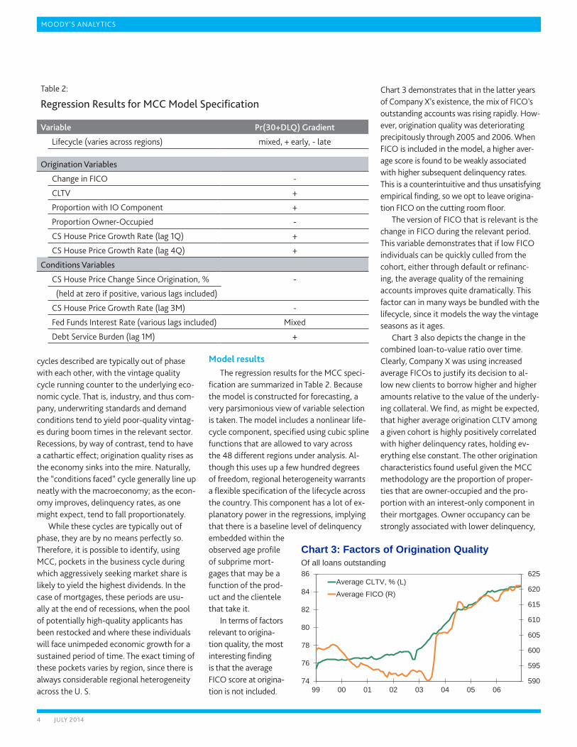
Chart 3 demonstrates that in the latter years of Company X’s existence, the mix of FICO’s outstanding accounts was rising rapidly. How-ever, origination quality was deteriorating precipitously through 2005 and 2006. When FICO is included in the model, a higher aver-age score is found to be weakly associated with higher subsequent delinquency rates. This is a counterintuitive and thus unsatisfying empirical finding, so we opt to leave origina-tion FICO on the cutting room floor.

The version of FICO that is relevant is the change in FICO during the relevant period. This variable demonstrates that if low FICO individuals can be quickly culled from the cohort, either through default or refinanc-ing, the average quality of the remaining accounts improves quite dramatically. This factor can in many ways be bundled with the lifecycle, since it models the way the vintage seasons as it ages.

Chart 3 also depicts the change in the combined loan-to-value ratio over time. Clearly, Company X was using increased average FICOs to justify its decision to al-low new clients to borrow higher and higher amounts relative to the value of the underly-ing collateral. We find, as might be expected, that higher average origination CLTV among a given cohort is highly positively correlated with higher delinquency rates, holding ev-erything else constant. The other origination characteristics found useful given the MCC methodology are the proportion of proper-ties that are owner-occupied and the pro-portion with an interest-only component in their mortgages. Owner occupancy can be strongly associated with lower delinquency,

33

590

595

600

605

610

615

620

625

74

76

78

80

82

84

86

99 00 01 02 03 04 05 06

Average CLTV, % (L)

Average FICO (R)

Chart 3: Factors of Origination QualityOf all loans outstanding

Table 2:

Regression Results for MCC Model Specification

Variable Pr(30+DLQ) Gradient

Lifecycle (varies across regions) mixed, + early, - late

Origination Variables

Change in FICO -

CLTV +

Proportion with IO Component +

Proportion Owner-Occupied -

CS House Price Growth Rate (lag 1Q) +

CS House Price Growth Rate (lag 4Q) +

Conditions Variables

CS House Price Change Since Origination, % -

(held at zero if positive, various lags included)

CS House Price Growth Rate (lag 3M) -

Fed Funds Interest Rate (various lags included) Mixed

Debt Service Burden (lag 1M) +

MOODY’S ANALYTICS

5 July 2014

implying that investor loans are more likely to turn sour, while IO loans are found to be more risky propositions.

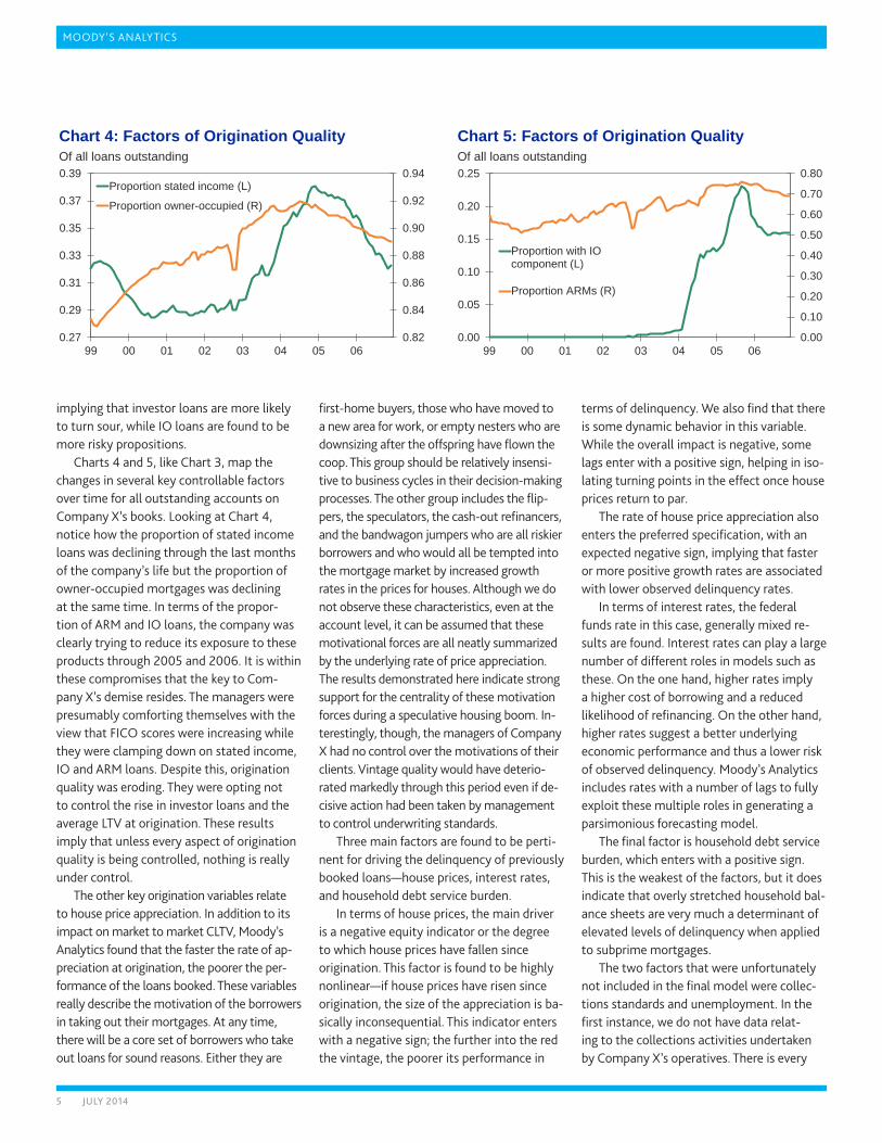
Charts 4 and 5, like Chart 3, map the changes in several key controllable factors over time for all outstanding accounts on Company X’s books. Looking at Chart 4, notice how the proportion of stated income loans was declining through the last months of the company’s life but the proportion of owner-occupied mortgages was declining at the same time. In terms of the propor-tion of ARM and IO loans, the company was clearly trying to reduce its exposure to these products through 2005 and 2006. It is within these compromises that the key to Com-pany X’s demise resides. The managers were presumably comforting themselves with the view that FICO scores were increasing while they were clamping down on stated income, IO and ARM loans. Despite this, origination quality was eroding. They were opting not to control the rise in investor loans and the average LTV at origination. These results imply that unless every aspect of origination quality is being controlled, nothing is really under control.

The other key origination variables relate to house price appreciation. In addition to its impact on market to market CLTV, Moody’s Analytics found that the faster the rate of ap-preciation at origination, the poorer the per-formance of the loans booked. These variables really describe the motivation of the borrowers in taking out their mortgages. At any time, there will be a core set of borrowers who take out loans for sound reasons. Either they are

first-home buyers, those who have moved to a new area for work, or empty nesters who are downsizing after the offspring have flown the coop. This group should be relatively insensi-tive to business cycles in their decision-making processes. The other group includes the flip-pers, the speculators, the cash-out refinancers, and the bandwagon jumpers who are all riskier borrowers and who would all be tempted into the mortgage market by increased growth rates in the prices for houses. Although we do not observe these characteristics, even at the account level, it can be assumed that these motivational forces are all neatly summarized by the underlying rate of price appreciation. The results demonstrated here indicate strong support for the centrality of these motivation forces during a speculative housing boom. In-terestingly, though, the managers of Company X had no control over the motivations of their clients. Vintage quality would have deterio-rated markedly through this period even if de-cisive action had been taken by management to control underwriting standards.

Three main factors are found to be perti-nent for driving the delinquency of previously booked loans—house prices, interest rates, and household debt service burden.

In terms of house prices, the main driver is a negative equity indicator or the degree to which house prices have fallen since origination. This factor is found to be highly nonlinear—if house prices have risen since origination, the size of the appreciation is ba-sically inconsequential. This indicator enters with a negative sign; the further into the red the vintage, the poorer its performance in

terms of delinquency. We also find that there is some dynamic behavior in this variable. While the overall impact is negative, some lags enter with a positive sign, helping in iso-lating turning points in the effect once house prices return to par.

The rate of house price appreciation also enters the preferred specification, with an expected negative sign, implying that faster or more positive growth rates are associated with lower observed delinquency rates.

In terms of interest rates, the federal funds rate in this case, generally mixed re-sults are found. Interest rates can play a large number of different roles in models such as these. On the one hand, higher rates imply a higher cost of borrowing and a reduced likelihood of refinancing. On the other hand, higher rates suggest a better underlying economic performance and thus a lower risk of observed delinquency. Moody’s Analytics includes rates with a number of lags to fully exploit these multiple roles in generating a parsimonious forecasting model.

The final factor is household debt service burden, which enters with a positive sign. This is the weakest of the factors, but it does indicate that overly stretched household bal-ance sheets are very much a determinant of elevated levels of delinquency when applied to subprime mortgages.

The two factors that were unfortunately not included in the final model were collec-tions standards and unemployment. In the first instance, we do not have data relat-ing to the collections activities undertaken by Company X’s operatives. There is every

44

0.82

0.84

0.86

0.88

0.90

0.92

0.94

0.27

0.29

0.31

0.33

0.35

0.37

0.39

99 00 01 02 03 04 05 06

Proportion stated income (L)

Proportion owner-occupied (R)

Chart 4: Factors of Origination QualityOf all loans outstanding

55

0.00

0.10

0.20

0.30

0.40

0.50

0.60

0.70

0.80

0.00

0.05

0.10

0.15

0.20

0.25

99 00 01 02 03 04 05 06

Proportion with IOcomponent (L)

Proportion ARMs (R)

Chart 5: Factors of Origination QualityOf all loans outstanding

MOODY’S ANALYTICS

6 July 2014

chance that some of the noise observed in the performance of the vintages could be explained by changes in internal manage-ment practices that were not included in the data used for this project. In terms of unemployment, meanwhile, it is found that labor market factors were generally unim-portant drivers of delinquency behavior. This may be a function of the era in which the bulk of our data were observed. Between 2003 and 2006, the unemployment rate was relatively static compared with the level of joblessness witnessed over the past year. One feels that if we had a data set through to the present day, from a surviving subprime lender—assuming such a firm could be lo-cated—it would show a stronger relationship between delinquency and fundamental labor market conditions.

A micro approachMoody’s Analytics fully recognizes the

utility that can be derived from loan level-based modeling approaches in the consumer credit industry.

First, relative to aggregate-based ap-proaches, lenders and investors may favor the loan level approach to modeling as invest-ment decisions and credit policies are often instituted at the loan level. A company origi-nating loans will accept or reject applications and set fees on a case-by-case basis. When an individual fills out an application form, the originator must score the application, ostensibly conducting a cost-benefit analysis, to decide whether the loan should be booked and under what terms. Further, an investor considering the purchase of a pool of whole loans will typically go through a portfolio and select certain loans for purchase while refus-ing others. Government banking and lending regulations may also require institutions to provide projections of default and losses at the account level for capital adequacy and stress-testing purposes. In some instances, financial reporting rules also require firms to mark or provide an individual value for each loan in their portfolio.

Individual level or micro-modeling of loan portfolios is clearly beneficial, since such an analysis provides details that a macro or ag-gregate level model simply cannot.

Since each individual loan within a portfolio may be defined by a multitude of risk factors and may be exposed to a variety of economic conditions, loan level models open up the pos-sibility of highly detailed and complex analysis of loan behavior. For example, individuals with a particular mix of characteristics may respond to collections activity in one way, while oth-ers with a different mix of characteristics may respond entirely differently. If one’s aim is to manage collections at such a granular level, loan level modeling approaches are neces-sary to achieve one’s objectives. Alternatively, recessions, such as that currently under way, may impact those with weak credit histories more acutely than those with rock-solid track records. If one were trying to identify at-risk individuals in the current environment, a detailed analysis of all individual loans in the portfolio, under a range of macroeconomic conditions, would be required.

If one is able to produce reasonable and sensible assumptions for each loan, then one need only sum across predictions in order to produce a portfolio level forecast. Whether this forecast is optimal given the available alternatives, including the MCC approach, is debatable and the subject of analysis in the current article. Consumer credit is perhaps the only arena in which individual level specifica-tions are sometimes preferred for forecasting over simpler, aggregate level approaches.

If the analyst, therefore, decides that the loan level models do not provide acceptable or optimal forecasts, this in no way diminish-es the other uses he or she may have for such specifications. Optimally, however, loan level models would provide predictions of portfo-lio performance aggregates that match those generated by the best available predictor. Ideally, scoring and micro-analysis would be conducted in a way that was consistent with optimal loss forecast methodologies. The only way to achieve such a consistent view is to make loan level scoring models slaves to optimal forecasting models, whatever form they happen to take.

The loan level modelGiven that outcomes of PDs are discrete

zero-one events, they may be estimated econometrically from the family of limited

dependent variable models that includes logit, probit, competing risk and proportional hazard models. The choice of technique for the modeling of loan level PDs depends on the precise definition of the problem under investigation and the nature of the data avail-able for estimation. For example, residential mortgages may be more susceptible to ter-mination from prepayment, in addition to default, than are bank cards. Therefore, a com-peting risk model where multiple outcomes are estimated jointly may be essential for the modeling of mortgages but unnecessary for the modeling of bank cards.

The treatment of time within PD models is another critical choice that the investiga-tor must make. In some instances, loans may be single-period contracts where money is borrowed and paid in full at a later date with a single payment. Such single-period, single-termination type models are easily addressed with binary logit or probit models. It is more often the case in consumer lend-ing that loans are repaid over time in regular installments. The choice of discrete time hazard models is common in PD modeling for this reason.

Once the relevant outcome variable and functional form of the PD model is estab-lished along with the appropriate treatment of time, the investigator must then deter-mine which explanatory variables or drivers should be included in the model. Standard economic theory is generally applied to se-lect a list of candidate variables from those that are available in the macroeconomic database. Explanatory variables generally fall into one of the “Four C’s of Credit”: charac-ter, capacity, capital and conditions. Char-acter might include such factors as previous credit usage and behavior. Capacity may be measured by debt-to-income ratios, which give an indication of the borrower’s ability to repay the debt after it is disbursed. Capital may be measured by a borrower’s net worth, liquid reserves, or the value of the underly-ing asset in the case of securitized lending such as a residential mortgage. Conditions may include variables such as a borrower’s employment status, health, or strength of the local housing market throughout the ex-pected life of the loan.

MOODY’S ANALYTICS

7 July 2014

It is relatively easy to measure and col-lect data on the first three of the C’s at the individual borrower level: Credit bureaus regularly collect information on the payment status of borrowers over time, and advanced credit scoring techniques exist to sum-marize the available wealth of information. Outstanding debts and income sources for a borrower are easily obtained and verified. Measures of wealth and asset values may be calculated, although values, especially future values, may be elusive, especially so given recent ructions in the housing market.

Individual borrower conditions, on the other hand, present a significant challenge. Ideally, one should include measures of the conditions specific to each individual bor-rower. For example, the probability of un-employment for an individual debtor—which takes into account his occupation, job tenure and education, among other things—would be an appropriate metric for the labor mar-ket conditions facing the borrower, which would have a direct impact on the likeli-hood he will continue to have the income stream needed to repay the loan. In the case of a residential mortgage, the current and projected value for the house securitiz-ing the loan would give an indication of the conditions under which the loan is being originated and the likelihood the borrower could sell the home to repay his debt rather than entering into default. Homeowners themselves do not know the true market value of their houses; it is folly to suggest that the lender, one step removed from the property, would be able to reliably measure the value of each house in the portfolio at a given point in time.

Unfortunately, such micro-level informa-tion is generally not available. More aggre-gated economic indicators such as the local unemployment rate within a metropolitan area are used as proxy variables for individual borrower conditions. Individual collateral values in the case of mortgage loans are also imprecisely measured. Given how infre-quently properties transact, the best that can be done is to estimate average growth pat-terns within a larger geography and assume that they apply to all properties equally within an area.

While these proxies may be better than nothing, they may not be particularly meaningful for predicting individual loan performance, as they are measured with substantial amounts of error. This issue and its consequences are well understood in the econometrics literature; its occurrence leads to a condition known as attenuation, which is the situation where, because of measure-ment error in the data, estimated elasticities are biased toward zero. The model’s esti-mated sensitivity to economic shocks and cycles will therefore be diminished relative to the level of sensitivity that actually exists in practice. This effect may be particularly pro-nounced for the proxy variables in loan level PD models where the importance of other loan level variables, measured with extreme-ly high precision, overwhelms the predictive power from the poorly measured economic conditions variables. Loan level variables, such as credit score, are also generally cor-related with the level of measurement error. Those with low scores, after all, suffer a higher probability of experiencing unemploy-ment in a given period relative to their peers with better credit track records.

Attenuation, as will be demonstrated, leads to a lack of cyclical sensitivity in loan level models such that they will tend to over-predict probabilities of default in good times and underpredict them in recessions such as the one currently raging.

Individual level resultsFor the individual loan level PD model,

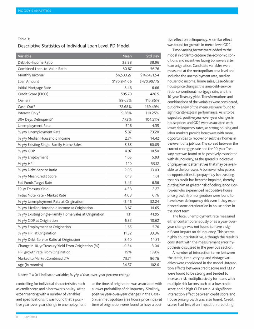
Moody’s Analytics estimated a standard logistic model on the discrete-time panel data, as used widely within the industry, conditional on the host of loan level and time-varying economic factors (see Table 3). Vintage level variables similar to those included in the aggregate level model were also tested, including year-over-year changes in unemployment, local GDP, and house price movements at the time of origination. Fixed effects were incorporated into the model as well to account for regional differences in delinquency performance above and beyond those captured by the other variables.

Candidate variables were introduced into the model with specifications consistent with

their measurement and potential impact on delinquency rates. Special attention was made to nonlinearities in the effects through the use of splines, categorical variables and interaction effects. A summary of the gradi-ent or directional impact of the variables on predicted delinquency rates is given in Table 4; the variables are described in the next section.

Included factorsA loan’s age defines the shape of the un-

derlying hazard function and is an extremely important determinant of delinquency prob-ability in the model. We typically find that the underlying hazard rate rises through the early years of a loan’s life as poor-quality credit risk individuals are gradually revealed. Over time, the cohort of lenders is thinned by attrition, and those left after a few years are typically higher than average-quality sur-vivors; as a result, the hazard starts to trend downward, albeit at a slower rate than its initial ascent.

Most static loan factors—typically characteristics of the borrower at origina-tion—entered the model with relationships to the probability of delinquency that were expected. For example, lower credit scores and higher debt-to-income ratios were as-sociated with a higher probability of delin-quency. The larger a borrower’s down pay-ment, the lower his CLTV ratio and the lower his probability of delinquency. The structure and terms of the loan also have an impact on performance. Interest-only, stated in-come documentation, cash-out refinancing, and 2/28 ARM loans are all associated with higher risk of delinquency. Other variables, such as an indicator for whether the loan car-ried a prepayment penalty and the lender’s internal risk grade score, were considered for inclusion in the model but were found to contribute little explanatory power, as these factors are correlated with other factors that are already in the model.

The economic conditions under which a loan was originated were found to have a permanent effect on future performance. For example, loans originated when underwriting quality was loose tended to perform worse throughout their lives compared with loans originated with tighter standards—even after

MOODY’S ANALYTICS

8 July 2014

controlling for individual characteristics such as credit score and a borrower’s equity. After experimenting with a number of variables and specifications, it was found that a posi-tive year-over-year change in unemployment

at the time of origination was associated with a lower probability of delinquency. Similarly, positive year-over-year changes in the Case-Shiller metropolitan area house price index at time of origination were found to have a posi-

tive effect on delinquency. A similar effect was found for growth in metro level GDP.

Time-varying factors were added to the model in order to capture the economic con-ditions and incentives facing borrowers after loan origination. Candidate variables were measured at the metropolitan area level and included the unemployment rate, median household income, home sales, Case-Shiller house price changes, the area debt-service ratio, conventional mortgage rate, and the 10-year Treasury yield. Transformations and combinations of the variables were considered, but only a few of the measures were found to significantly explain performance. As is to be expected, positive year-over-year changes in house prices and GDP were associated with lower delinquency rates, as strong housing and labor markets provide borrowers with more opportunities to recover or sell their homes in the event of a job loss. The spread between the current mortgage rate and the 10-year Trea-sury rate was found to be positively associated with delinquency, as the spread is indicative of prepayment alternatives that may be avail-able to the borrower. A borrower who passes up opportunities to prepay may be revealing that his credit has become impaired, thereby putting him at greater risk of delinquency. Bor-rowers who experienced net positive house price growth from origination were found to have lower delinquency risk even if they expe-rienced some deterioration in house prices in the short term.

The local unemployment rate measured either contemporaneously or as a year-over-year change was not found to have a sig-nificant impact on delinquency. This seems highly counterintuitive, although the result is consistent with the measurement error hy-pothesis discussed in the previous section.

A number of interaction terms between the static, time-varying and vintage vari-ables were considered in the model. Interac-tion effects between credit score and CLTV were found to be strong and tended to increase risk multiplicatively for loans with multiple risk factors such as a low credit score and a high CLTV ratio. A significant interaction effect between credit score and house price growth was also found. Credit scores had less of an impact on predicting

Table 3:

Descriptive Statistics of Individual loan level PD Model

Variable Mean Std Dev

Debt-to-Income Ratio 38.88 38.96

Combined Loan-to-Value Ratio 80.67 56.76

Monthly Income $6,533.27 $167,421.54

Loan Amount $170,841.06 $470,907.75

Initial Mortgage Rate 8.46 6.66

Credit Score (FICO) 595.79 426.5

Owner? 89.65% 115.86%

Cash-Out? 72.68% 169.49%

Interest Only? 9.26% 110.25%

30+ Days Delinquent? 7.73% 104.51%

Unemployment Rate 5.16 4.35

% y/y Unemployment Rate 5.37 73.20

% y/y Median Household Income 2.74 14.42

% y/y Existing Single-Family Home Sales -5.65 60.05

% y/y GDP 4.97 10.50

% y/y Employment 1.05 5.93

% y/y HPI 1.10 53.12

% y/y Debt-Service Ratio 2.05 13.03

% y/y Mean Credit Score 0.13 1.61

Fed Funds Target Rate 3.45 6.56

10-yr Treasury Yield 4.38 2.27

Initial Note Rate - Market Rate 4.08 6.76

% y/y Unemployment Rate at Origination -3.46 52.24

% y/y Median Household Income at Origination 3.67 14.65

% y/y Existing Single-Family Home Sales at Origination 1.11 41.95

% y/y GDP at Origination 6.32 10.62

% y/y Employment at Origination 1.65 5.76

% y/y HPI at Origination 11.32 33.36

% y/y Debt-Service Ratio at Origination 2.40 14.21

Change in 10-yr Treasury Yield From Origination (%) -0.34 3.04

HPI growth rate From Origination 19% 139%

Marked to Market Combined LTV 73.74 96.76

Age (in months) 34.57 102.6

Notes: ? = 0/1 indicator variable; % y/y = Year-over-year percent change

MOODY’S ANALYTICS

9 July 2014

delinquency performance at either extreme of house price growth, which is reasonable, as a strong economy will hide the weak-ness of lower credit borrowers, while in a sharply declining economy, even high credit

borrowers will be affected by job losses and shrinking incomes.

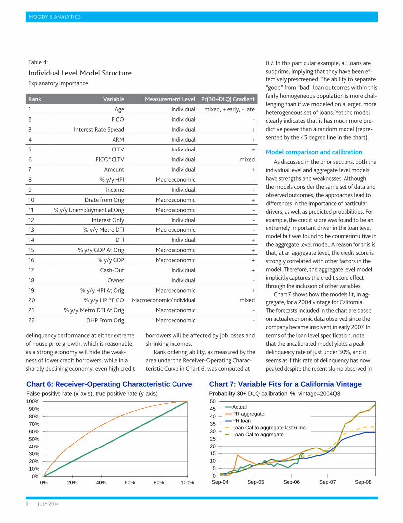
Rank ordering ability, as measured by the area under the Receiver-Operating Charac-teristic Curve in Chart 6, was computed at

0.7. In this particular example, all loans are subprime, implying that they have been ef-fectively prescreened. The ability to separate “good” from “bad” loan outcomes within this fairly homogeneous population is more chal-lenging than if we modeled on a larger, more heterogeneous set of loans. Yet the model clearly indicates that it has much more pre-dictive power than a random model (repre-sented by the 45 degree line in the chart).

Model comparison and calibrationAs discussed in the prior sections, both the

individual level and aggregate level models have strengths and weaknesses. Although the models consider the same set of data and observed outcomes, the approaches lead to differences in the importance of particular drivers, as well as predicted probabilities. For example, the credit score was found to be an extremely important driver in the loan level model but was found to be counterintuitive in the aggregate level model. A reason for this is that, at an aggregate level, the credit score is strongly correlated with other factors in the model. Therefore, the aggregate level model implicitly captures the credit score effect through the inclusion of other variables.

Chart 7 shows how the models fit, in ag-gregate, for a 2004 vintage for California. The forecasts included in the chart are based on actual economic data observed since the company became insolvent in early 2007. In terms of the loan level specification, note that the uncalibrated model yields a peak delinquency rate of just under 30%, and it seems as if this rate of delinquency has now peaked despite the recent slump observed in

Table 4:

Individual level Model StructureExplanatory Importance

Rank Variable Measurement Level Pr(30+DLQ) Gradient

1 Age Individual mixed, + early, - late

2 FICO Individual -

3 Interest Rate Spread Individual +

4 ARM Individual +

5 CLTV Individual +

6 FICO*CLTV Individual mixed

7 Amount Individual +

8 % y/y HPI Macroeconomic -

9 Income Individual -

10 Drate from Orig Macroeconomic +

11 % y/y Unemployment at Orig Macroeconomic -

12 Interest Only Individual -

13 % y/y Metro DTI Macroeconomic -

14 DTI Individual +

15 % y/y GDP At Orig Macroeconomic +

16 % y/y GDP Macroeconomic +

17 Cash-Out Individual +

18 Owner Individual -

19 % y/y HPI At Orig Macroeconomic +

20 % y/y HPI*FICO Macroeconomic/Individual mixed

21 % y/y Metro DTI At Orig Macroeconomic -

22 DHP From Orig Macroeconomic -

66

Chart 6: Receiver-Operating Characteristic CurveFalse positive rate (x-axis), true positive rate (y-axis)

0%10%20%30%40%50%60%70%80%90%

100%

0% 20% 40% 60% 80% 100%

77

05

101520253035404550

Sep-04 Sep-05 Sep-06 Sep-07 Sep-08

ActualPR aggregatePR loanLoan Cal to aggregate last 6 mo.Loan Cal to aggregate

Chart 7: Variable Fits for a California VintageProbability 30+ DLQ calibration, %, vintage=2004Q3

MOODY’S ANALYTICS

10 July 2014

the macroeconomy. The two different models track each other quite closely through 2007, but the picture changes dramatically in 2008 as the economy worsens. The delinquency rate predicted by the MCC model shows a sharp uptick in the delinquency rate and hits close to 50% in the current period. We know from ex-perience working with securitized data, includ-ing many mortgages originated by Company X, that 50% short-term delinquency rates are not uncommon for subprime mortgages of a similar vintage. The fact that this chart pertains to California, the epicenter of the subprime crisis, means that, if anything, 50% is too low a predicted rate given current conditions. A figure of 30% more closely compares to a foreclosure rate for these types of mortgages. The company might have been able to survive a 30% peak California delinquency rate.

One of the Moody’s Analytics models is designed for forecasting and to accurately re-flect the effect of business cycles on portfolio performance, while the other is designed for classification and scoring of individual loans based on borrower characteristics. Ideally, we desire to create a model that can lever-age the strengths of both approaches while minimizing the weaknesses. A calibration procedure is proposed in the next section that achieves this objective.

Traditional calibration approachBy their nature, all econometric models

have errors. Variables are measured impre-cisely and human behavior has a random component that at times will defy logic and reason. The economy is also constantly shift-ing and evolving such that relationships be-tween variables and predicted outcomes will move over time. Econometric analysis will look to discover the long-term stable rela-tionships, leaving the potential for some de-gree of prediction error in the short term. As loss forecasting exercises are concerned with short-term as well as long-run predictions, calibration is used to minimize the likelihood and magnitude of short-run forecast error.

The traditional approach to calibration is to compare predicted versus actual rates in sample after the model has been estimated and then determine add factors or multipli-ers in order to better align predicted prob-

abilities with realized performance. Typical approaches include:

» 1. Adding calendar time effects (dum-mies) to the model and re-estimating. This will achieve perfect fit by period within sample by design but begs the question of how to carry forward the adjustment in the out-of-sample pe-riod. Application of the method would require the analyst to forecast the time effects using a separate model that may suffer some serious econo-metric specification errors.

» 2. Calibrate to the error from the last n observed periods. For example, if the predicted value is off by 10%, on aver-age, for the last six periods, one could assume that errors of this magnitude persist through the forecast period. The benefit of the approach is that it is anchored to the most recent available data. However, the error in the last few periods could be idiosyncratic rather than indicative of future prediction er-rors. This could lead to volatile and un-stable predictions in the out-of-sample period. The analyst would also need to make some assumptions regarding the persistence of the error correction. Should it continue indefinitely? Should it decay? If so, after how many periods and with which speed?

Chart 7 gives an example of the second calibration procedure, assuming n=6, ap-plied to the California cohort mentioned earlier. The predicted approach results in an increased predicted delinquency rate but still only a 33% peak delinquency rate. However, if the model happened to have been over-predicting rather than underpredicting in the last six observed periods, calibration would have resulted in an even lower predicted peak probability of delinquency. In part, the calibration simply reflects noisiness in the observed data.

In addition to the volatility and subjectiv-ity of the calibrations, another issue is that they are backward-looking level shifts. They do not capture forward-looking dynam-ics around the model error. One possibility along these lines would be to take the esti-mated calendar month effects from option 1

and model them against exogenous macro-economic factors (assuming these factors are forecasted). Such a two-stage method would be an improvement over simple calibration approaches, although it would fail to capture the interactions between the loan level fac-tors and the macroeconomy. This is precisely the motivation for the aggregate modeling approach embodied by MCC.

The micro-macro calibration approachAlternatively, the loan level model can be

calibrated not to observed history but to the forecasts generated by the aggregate, MCC model. Under the assumption that the ag-gregate model provides a superior forecast for the performance of existing and future vin-tages, we may calibrate the micro model such that the summed outcomes of the calibrated individual level model equal the aggregate model’s predictions at a given point in time.

The specification of the calibration ad-justment factor can take a variety of forms and is dependent on the intended usage and need of the modeled output. Consider-ations of timing and segmentation affect the complexity of the factor and whether it is a simple additive or multiplicative factor or if it is a function of the PD at different points in time accounting for correlations among modeled segments.

The superiority of micro-macro calibra-tion over the traditional approach is obvious along three key dimensions:

» 1. The traditional approach has a his-torical bias: The oldest vintages with the longest observed performance his-tory dominate within the traditional approach. However, the most recently originated or newest vintages are of-ten the most important in determining future overall portfolio performance. By calibrating to forecasts, including forecasts of current and future vin-tages, an approach is developed that has no clear historical bias.

» 2. The alternative approach leverages the aggregate model: As discussed previously, a major advantage of the aggregate modeling approach is that it provides a forecast for both older and more recently originated loans as well

MOODY’S ANALYTICS

11 July 2014

as future vintages of loans. Forecasts for new vintages are possible, as the aggregate model is able to incorporate the credit and business cycles more explicitly in the model.

» 3. Forward-looking information provides a better forecast: Calibration of the loan level model to the aggregate level mod-el provides a more elegant and robust mechanism for incorporating forward-looking macroeconomic forecasts than the traditional calibration method. The aggregate model allows for the incorpo-ration of broader correlations and feed-back effects that the loan level model is unable to handle on its own.

Using a forecast as the basis for calibra-tion helps to overcome many of the primary problems associated with using loan level PD models, without losing any of the benefits. The rank ordering provided by loan level specifications is unaffected by the calibration procedure, though relative credit risk may shift as macroeconomic factors are tuned in. For example, suppose that John’s probability of default, in a boom, is twice as high as that of Mary. One would expect that John, with weak-er personal characteristics, would be more acutely affected by the onset of recession than Mary. An optimal loan level model should

reflect this stretching of the population when faced with severe downside stresses.

Summary and conclusionThe availability of data on Company X

permitted Moody’s Analytics to compare the traditional loan level approach with loss forecasting to an alternative aggregate modeling approach. It is observed that the loan level micro model captures the rank or-dering of risk well and that the relative rank ordering of the model based on loan-specific factors is reasonably stable over time. The aggregate or macro model is able to better predict the overall performance level for a portfolio of loans as it captures vintage origi-nation, credit and business cycles explicitly, along with correlations between borrowers and macroeconomic feedback effects. An ad-ditional advantage of the aggregate model is that its relatively simple structure allows it to be quickly updated and re-estimated as policy and data change. The loan level model is much more complex and would require greater oversight to ensure that changes feed through the system properly. Calibration of the two models provides a best-in-class, state-of-the-art approach to loss forecasting and modeling. Appropriate definition of the calibration adjustment factor allows for a

model that can capture loan level rank order-ing of risk while allowing for the impact of broader macroeconomic and systemic risks to be fully reflected in the model’s forecasts.

In terms of the management failures that led to Company X’s demise, a number of fac-tors were identified that, while important in individual credit decisioning, turned out to yield counterintuitive effects when applied at a broader portfolio level. Had managers of Company X targeted factors such as CLTV, owner occupancy, and IO loan concentration and been less concerned with FICO scores, they may have originated better-quality vin-tages in 2005 and 2006 and thus improved their overall chances of survival.

Given the depth of the economic mire experienced over the past year, however, Com-pany X probably would have been a victim of the actions of other lenders in the industry even if its managers had pulled all the right levers back in 2005 and 2006. Because MCC considers factors under the control of portfolio managers, together with industry and econo-my-wide factors, the methodology would have predicted gloomy numbers as soon as precipi-tous house price declines became likely. Given such a forecast, a graceful early exit from the industry may have been the only sensible ac-tion available for Company X’s investors.

MOODY’S ANALYTICS

About the Author Cristian de Ritis is senior director at Moody’s Analytics. He performs consumer credit modeling and analysis with the firm’s Credit Analytics group and contributes to the analysis for CreditForecast.com. Before joining the Moody’s Analytics West Chester PA operation, Cris worked for Fannie Mae and taught at Johns Hopkins University in Washington DC. He received a PhD and MA in economics from Johns Hopkins University and graduated summa cum laude from Michigan State University with a bach-elor’s degree in economics.

Tony Hughes is managing director of Credit Analytics at Moody’s Analytics, where he manages the company’s credit analysis consulting projects for global lending institu-tions. An expert applied econometrician, Dr. Hughes also oversees the Moody’s CreditCycle and manages CreditForecast.com. His varied research interests have lately focused on problems associated with loss forecasting and stress-testing credit portfolios.

Now based in the U.S., Dr. Hughes previously headed the Moody’s Analytics Sydney office, where he was editor of the Asia-Pacific edition of the Dismal Scientist web site and was the company’s lead economist in the region. He retains a keen interest in emerging markets and in Asia-Pacific economies.

A former academic, Dr. Hughes held positions at the University of Adelaide, the University of New South Wales, and Vanderbilt University and has published a number of articles in leading statistics and economics journals. He received his PhD in econometrics from Monash University in Melbourne, Australia.

MOODY’S ANALYTICS

About Moody’s Analytics

Moody’s Analytics helps capital markets and credit risk management professionals worldwide respond to an evolving

marketplace with confi dence. With its team of economists, the company offers unique tools and best practices for

measuring and managing risk through expertise and experience in credit analysis, economic research, and fi nancial

risk management. By offering leading-edge software and advisory services, as well as the proprietary credit research

produced by Moody’s Investors Service, Moody’s Analytics integrates and customizes its offerings to address specifi c

business challenges.

Concise and timely economic research by Moody’s Analytics supports fi rms and policymakers in strategic planning, product and sales forecasting, credit risk and sensitivity management, and investment research. Our economic research publications provide in-depth analysis of the global economy, including the U.S. and all of its state and metropolitan areas, all European countries and their subnational areas, Asia, and the Americas. We track and forecast economic growth and cover specialized topics such as labor markets, housing, consumer spending and credit, output and income, mortgage activity, demographics, central bank behavior, and prices. We also provide real-time monitoring of macroeconomic indicators and analysis on timely topics such as monetary policy and sovereign risk. Our clients include multinational corporations, governments at all levels, central banks, fi nancial regulators, retailers, mutual funds, fi nancial institutions, utilities, residential and commercial real estate fi rms, insurance companies, and professional investors.

Moody’s Analytics added the economic forecasting fi rm Economy.com to its portfolio in 2005. This unit is based in West Chester PA, a suburb of Philadelphia, with offi ces in London, Prague and Sydney. More information is available at www.economy.com.

Moody’s Analytics is a subsidiary of Moody’s Corporation (NYSE: MCO). Further information is available at www.moodysanalytics.com.

About Moody’s Corporation

Moody’s is an essential component of the global capital markets, providing credit ratings, research, tools and analysis that contribute to transparent and integrated fi nancial markets. Moody’s Corporation (NYSE: MCO) is the parent company of Moody’s Investors Service, which provides credit ratings and research covering debt instruments and securities, and Moody’s Analytics, which encompasses the growing array of Moody’s nonratings businesses, including risk management software for fi nancial institutions, quantitative credit analysis tools, economic research and data services, data and analytical tools for the structured fi nance market, and training and other professional services. The corporation, which reported revenue of $3.5 billion in 2015, employs approximately 10,400 people worldwide and maintains a presence in 36 countries.

© 2016, Moody’s Analytics, Moody’s, and all other names, logos, and icons identifying Moody’s Analytics and/or its products and services are trademarks of Moody’s Analytics, Inc. or its affi liates. Third-party trademarks referenced herein are the property of their respective owners. All rights reserved. ALL INFORMATION CONTAINED HEREIN IS PROTECTED BY COPYRIGHT LAW AND NONE OF SUCH INFORMATION MAY BE COPIED OR OTHERWISE REPRODUCED, REPACKAGED, FURTHER TRANSMITTED, TRANSFERRED, DISSEMINATED, REDISTRIBUTED OR RESOLD, OR STORED FOR SUBSEQUENT USE FOR ANY PURPOSE, IN WHOLE OR IN PART, IN ANY FORM OR MANNER OR BY ANY MEANS WHATSOEVER, BY ANY PERSON WITHOUT MOODY’S PRIOR WRITTEN CONSENT. All information contained herein is obtained by Moody’s from sources believed by it to be accurate and reliable. Because of the possibility of human and mechanical error as well as other factors, however, all information contained herein is provided “AS IS” without warranty of any kind. Under no circumstances shall Moody’s have any liability to any person or entity for (a) any loss or damage in whole or in part caused by, resulting from, or relating to, any error (negligent or otherwise) or other circumstance or contingency within or outside the control of Moody’s or any of its directors, offi cers, employees or agents in connection with the procurement, collection, compilation, analysis, interpretation, communication, publication or delivery of any such information, or (b) any direct, indirect, special, consequential, compensatory or incidental damages whatsoever (including without limitation, lost profi ts), even if Moody’s is advised in advance of the possibility of such damages, resulting from the use of or inability to use, any such information. The fi nancial reporting, analysis, projections, observations, and other information contained herein are, and must be construed solely as, statements of opinion and not statements of fact or recommendations to purchase, sell, or hold any securities. NO WARRANTY, EXPRESS OR IMPLIED, AS TO THE ACCURACY, TIMELINESS, COMPLETENESS, MERCHANTABILITY OR FITNESS FOR ANY PARTICULAR PURPOSE OF ANY SUCH OPINION OR INFORMATION IS GIVEN OR MADE BY MOODY’S IN ANY FORM OR MANNER WHATSOEVER. Each opinion must be weighed solely as one factor in any investment decision made by or on behalf of any user of the information contained herein, and each such user must accordingly make its own study and evaluation prior to investing.