Publication No. 100

ANALYSIS OF WATER SUPPLY PROBLEMS USING MICROCOMPUTERS

by

Michael A. Moore

UNIVERSITY OF FLORIDA Gainesville, Florida 32611

Publication No. 100

FLORIDA WATER RESOURCES RESEARCH CENTER

ANALYSIS OF WATER SUPPLY PROBLEMS USING MICROCOMPUTERS

BY

MICHAEL A. MOORE

A THESIS PRESENTED TO THE GRADUATE SCHOOL OF THE UNIVERSITY OF FLORIDA IN

PARTIAL FULFILLMENT OF THE REQUIREMENTS FOR THE DEGREE OF MASTER OF SCIENCE

UNIVERSITY OF FLORIDA

1987

TABLE OF CONTENTS

ACKNOWLEDGEMENTS

LIST OF TABLES . . .

LIST OF FIGURES

ABSTRACT

CHAPTERS

I INTRODUCTION

II THE LOTUS 123 ELECTRONIC SPREADSHEET

Introduction . . . Literature Review Macros . . . . . .

III PRELIMINARY WATER TREATMENT DESIGN AND COST ESTIMATION . . . . . . . . . . .

Introduction . . . . . . Decision Support System WATERMAID Program . . . Lotus 123 WTRMAID Program

WTRMAID Menu . . . . . . . . . . . . . . . . Knowledge Bases . . . .. ....... . Execution . . . . . . . . ..... . . . Spreadsheet Protection . . . . . . . . . . . Macros . . . . . . . . . . . . . . . Calculations . . . . . . . . . . . . Data Tables and Graphs . . .

Conclusions

IV PRE- AND POSTPROCESSORS FOR A HYDRAULIC PIPE

ii

vi

ix

x

1

4

4 6 6

7

7 7 8 9

9 21 23 24 24 26 27

27

NETWORK ANALYSIS MODEL . . . . . . . . . .. 32

Introduction . . . . . . . . . . . . . . . . 32 Lotus 123 Pre- and Postprocessors . . . . . .. 33 Computer Analysis of Flow in Pipe Networks . 34

iii

CHAPTERS Page

Mass Continuity and Energy Conservation Equations . . . . . . . . . . . . . . .. 36

Linear Method . ............. 39 Solution of the Linear Method Using

Lotus 123 .... . . . . . . . . . . .. 41 Solving a Set of Simultaneous Equations

Using Matrix Techniques . . . . . . . .. 46 Additional Features in Wood's Model. . . .. 62

Lotus 123 Preprocessor .

Menu . . . . . . . . Spreadsheet Protection Error and Help Messages . . . Help Menu . . . . . . . . Additional Program Features . Macro . . . . . . . .

Lotus 123 Postprocessor

Menu . . . . . . . . Additional Features .

Conclusions

V OPTIMAL ADJUSTMENTS IN ERRONEOUS HYDRAULIC

62

64 65 65 66 66 68

70

70 72

74

NETWORK FLOWS . . . . . . . . . . .. 76

Introduction ....... ..... .. 76 Least Errors Squared Network Optimization . .. 77 Optimization of the Network Using Lotus 123 78 Network Optimization Using Linear Programming 81 Comparison of Three Optimization Strategies 92

Least Errors Squared Analysis . Least Absolute Value Analysis Minimizing the Maximum Error

Optimization of Networks Involving Gross Errors . . . . . . . . . . . . . . .

Gross Error Detection Algorythms . . . .

94 94 98

99 99

Measurement Test . . . . . . . . .. 109 Modified Iterative Measurement Test . . . .. 110 Pseudonodes Test . . . . . . . . . . . . .. 110 Combinatorial Test . . . . . .. .... 111 Screened Combinatorial Test . .. .... 112 Comparison of the Five Algorithms 112

iv

CHAPTERS Page

Solving the Modified Iterative Measurement Test Using Lotus 123 ............ 113

Comparison of Network Optimization with and without Error Detection ..... 116

Conclusions . . . . .. .......... 116

VI SUMMARY AND CONCLUSIONS

Objectives . . . . . . . . . . . Electronic Spreadsheets . .. ... Decision Support System . .. .. . Data Handling . . . . . . . Spreadsheet Modeling . .. .... . Conclusions . . . . . . . . . . Suggestions for Additional Investigations

APPENDICES

A HELP SECTIONS IN WTRMAID PROGRAM . .

122

122 122 123 124 124 125 126

127

B EXECUTED OUTPUT FROM EXAMPLE WTRMAID PROGRAM 132

C MACROS IN WTRMAID PROGRAM 137

D PH ITERATION CALCULATION IN RAPID MIX PROCESS OF WTRMAID PROGRAM . . . . . . . . . . . .. 140

E DATA REQUIRED TO PRODUCE LOGARITHMIC GRAPH IN WTRMAID PROGRAM . . . . . . . . . . . . . .. 142

F INPUT SECTIONS IN SPREADSHEET PREPROCESSOR FOR WOOD'S MODEL .......... . 147

G HELP MESSAGES IN PREPROCESSOR FOR WOOD'S MODEL. 150

H DATA CARDS IN SPREADSHEET PREPROCESSOR FOR WOOD'S MODEL . . . . . .... 155

I MACROS IN SPREADSHEET PRE- AND POSTPROCESSORS FOR WOOD'S MODEL . . . . . . . . .. 157

REFERENCES . 160

BIOGRAPHICAL SKETCH 163

v

LIST OF TABLES

Table

3-1 Treatment Process Section in WTRMAID Program

3-2 Influent Water Properties section in Program . . . . . . . . . . . . .

3-3 Cost Factors section in WTRMAID Program .

3-4 Cost of Chemicals section in WTRMAID

3-5

3-6

3-7

3-8

4-1

4-2

4-3

4-4

4-5

4-6

4-7

4-8

Program

Contaminant Section in WTRMAID Program

stream/Process Map section in WTRMAID Program . . . . . . . . . . . . . .

Flocculation Process Data Input Section in WTRMAID Program . . . . . . . . .

Data Table 1 in WTRMAID Program .

Physical Characteristics for pipes in Figure 4-1 . . . . . . . . . . . .

Calculation of Kp, Km, and Z for Pipes in Figure 4-1 . . . • . . .. .••.

Calculation of Qi, Hi, and Gi for Pipes in Figure 4-1 . . . . . . . .

Calculation of Summation of Gi*Qi

Matrix for Solving Simultaneous Equations

Second Iteration of Linear Method

Third Iteration of Linear Method

Fourth Iteration of Linear Method .

vi

12

13

15

16

17

19

22

28

42

43

44

45

47

48

51

54

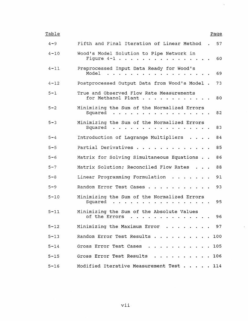
Table Page

4-9 Fifth and Final Iteration of Linear Method 57

4-10 Wood's Model Solution to Pipe Network in Figure 4-1 . . . . . . . . 60

4-11 Preprocessed Input Data Ready for Wood's Model . . . . . . . . 69

4-12 Postprocessed output Data from Wood's Model. 73

5-1 True and Observed Flow Rate Measurements for Methanol Plant ........ 80

5-2 Minimizing the Sum of the Normalized Errors Squared . . . .. .......... 82

5-3 Minimizing the Sum of the Normalized Errors Squared . .. .......... 83

5-4 Introduction of Lagrange Multipliers 84

5-5 Partial Derivatives . . . . . . 85

5-6 Matrix for Solving Simultaneous Equations 86

5-7 Matrix Solution; Reconciled Flow Rates 88

5-8 Linear Programming Formulation 91

5-9 Random Error Test Cases . 93

5-10 Minimizing the Sum of the Normalized Errors Squared . . . .. ........ 95

5-11 Minimizing the Sum of the Absolute Values of the Errors . . . . • . 96

5-12 Minimizing the Maximum Error 97

5-13 Random Error Test Results . . 100

5-14 Gross Error Test Cases . . . 105

5-15 Gross Error Test Results . . 106

5-16 Modified Iterative Measurement Test . . . 114

vii

Table

5-17

5-18

5-19

Modified Iterative Measurement Test .

Page

. 117

Modified Iterative Measurement Test . . . . . 118

Comparison with and without Error Detection . 119

viii

Figure

3-1

3-2

4-1

4-2

4-3

5-1

5-2

5-3

LIST OF FIGURES

Spreadsheet Diagram of WTRMAID Program

Modified Iterative Measurement Test .

water Distribution Network . . . . .

Spreadsheet Diagram of Wood's Model Preprocessor . . . . . . . . . . .

Spreadsheet Diagram of Wood's Model Postprocessor . . . . .

Methanol Steam Plant Network .

Waste Water Collection Network

Nodal Aggregate to Eliminate Stream X4045

ix

10

29

35

63

71

79

90

115

Abstract of Thesis Presented to the Graduate School of the University of Florida in Partial Fulfillment of the

Requirements for the Degree of Master of Science

ANALYSIS OF WATER SUPPLY PROBLEMS USING MICROCOMPUTERS

By

Michael A. Moore

August, 1987

Chairman: James P. Heaney Major Department: Environmental Engineering Sciences

Improvements in the microcomputer and ever more

sophisticated software packages allow a person to solve

water supply problems today that could only be solved with

larger computers previously. A solution to three water

supply problems is sought through the use of the micro-

computer and three software programs.

The first water supply problem deals with improving the

knowledge base structure of a model which determines

preliminary design and cost estimates for various potable

water treatment processes. The second problem involves

improving the efficiency in handling both input and output

data associated with a model which analyzes flow in pipe

networks. The third problem concerns the optimization of

water distribution networks that include erroneous flows

within the network.

x

An electronic spreadsheet is used throughout in solving

the water supply problems. The spreadsheet effectively

replaces hand calculation methods to solve these water

supply problems that could not be solved using a micro­

computer five years ago. A computer programming language

called macro is used extensively within the spreadsheets to

create programs for problem solution that are fast, flex­

ible, and simple to use. Macros are written to create a

menu system which allows even the novice to operate the

programs while knowledge bases, help systems, and logical

data handling capabilities are included for ease of opera­

tion.

xi

CHAPTER I INTRODUCTION

The microcomputer, combined with existing software, is

becoming an increasingly powerful tool for solving environ-

mental engineering problems. until recently, when micro-

computers began to be used, most automated computation was

performed on large general-purpose computers, using remote

terminals. The microcomputer offers the alternative of a

small, inexpensive desk-top work station. The user can

perform small tasks on microcomputers more efficiently and

cost effectively than on large computers.

This is not to say that microcomputers will eventually

replace large computers. The main-frame user may find it

easier to use the microcomputer to more logically understand

the problem at hand before delving into the larger computer.

The most effective way of using the various sizes of

available computers is to fit them to the tasks they are to

perform instead of trying to perform all tasks on large,

general-purpose computers. with improvements in the

available software, microcomputers are able to solve ever

more technical engineering problems.

The objective of this thesis is to demonstrate the ever

expanding role of the microcomputer using existing software,

more specifically the Lotus 123 electronic spreadsheet, to

1

2

solve water distribution and treatment problems. Three

software packages are used to solve three different water

distribution and treatment problems. The software includes

an electronic spreadsheet, a linear programming model, and a

model for computer analysis of flow in pipe networks.

Chapter II gives a general background on electronic

spreadsheets. Lotus 123, Release 2, is chosen as it is the

most popular electronic spreadsheet available at this time.

The explanation of the Lotus 123 spreadsheet will be brief

as the reader is invited to read a thesis by Hancock (1986)

for a description of the evolution of the microcomputer and

use of the Lotus 123 electronic spreadsheet in water

resources.

Chapter III applies Lotus 123 to create a decision

support system for the preliminary design and cost estima­

tion of municipal potable water treatment. A newly devel­

oped interactive program written in the BASIC computer

language, called WATERMAID, already exists for this purpose.

An attempt is made to improve upon the knowledge base

structure of this program using Lotus 123.

Chapter IV demonstrates the capability and advantages

of using Lotus 123 in a data management role. Lotus 123 is

used to create a spreadsheet program for the pre- and

postprocessing of data used in a model for computer analysis

of flow in pipe networks. The majority of time spent in the

use of existing pipe network models is in the processing of

the initial data to be used in the model and the final

output data. The pre- and postprocessors are designed to

speed the data management process.

3

Chapter V applies existing methods used by chemical

engineers in the optimization of erroneous flows in indus­

trial process networks to the field of water distribution

networks. Lotus 123 is used to demonstrate the methods,

which are presently used on much larger computer systems, on

the microcomputer. In addition, two linear programming

methods to achieve this optimization process are introduced.

The summary and conclusions are found in Chapter VI.

In addition, Chapter VI includes possibilities for further

research in this area.

CHAPTER 11 THE LOTUS 123 ELECTRONIC SPREADSHEET

Introduction

Electronic spreadsheets are one of the more popular

software produced at this time and Lotus 123 is the most

popular of the electronic spreadsheets. The Lotus 123

electronic spreadsheet can be described as a large matrix of

cells, 254 columns by 8192 rows, and can be visualized as a

large electronic piece of paper. Instead of using a writing

instrument and a piece of paper to accomplish calculations,

the Lotus 123 user uses the computer keyboard to make

entries and views only a portion of the large electronic

spreadsheet on the monitor. In other words, with the Lotus

123 spreadsheet, the engineer can put away the engineering

paper, pencil, and hand held calculator.

The user of the Lotus 123 spreadsheet is able to employ

a myriad of commands and functions which make the spread-

sheet a very powerful and versatile tool for solving

engineering problems (LeBlond and Cobb, 1985; Lotus

Development Corporation, 1985; Gregory, 1986). Special

mathematical, statistical, data management and logical

functions can be accessed for use in the spreadsheet.

Graphs can be produced from data involving X and Y

4

coordinates. Even maps and figures can be produced using

Lotus 123.

An important advantage of Lotus 123 is that the user

does not need to learn a programming language. The spread­

sheet can be used to duplicate many programs produced using

a programming language such as BASIC or FORTRAN. Only a

minimum of commands needs to be learned initially to get

started.

5

One of the problems in using a conventional program,

say written in the BASIC language, is that the user is

working with a sort of "black box". In an interactive

program the user is prompted to input certain data and when

the program is executed, final computations are output. The

user is normally not privy to what is going on inside the

black box so the user does not clearly understand how the

output is derived from the input.

Both calculations and text can be integrated into the

spreadsheet. Using Lotus 123, all reference documentation

in the form of equations, assumptions, data tables, graphs,

maps, and figures can be included on the spreadsheet in an

organized manner, thereby eliminating the black box. The

documentation can be easily updated as advances in the

knowledge base are made. Having the knowledge base inte­

grated into the spreadsheet reduces the time and energy

spent locating any required reference material and allows

the user to quickly make intelligent decisions regarding

parameter estimates that need to be input to the program.

6

Literature Review

The use of microcomputers and customized software

programs in both the municipal sewer system (Calise et al.,

1984; Cullen and Murrell, 1985) and potable water treatment

and distribution systems (Harris, 1984; Koh & Maidment,

1984) provides a solution to the time consuming and tedious

engineering problems of analysis, design and costing. In

addition, engineering design is becoming more efficient as

hand calculations are replaced by computer automated design.

Macros

The Lotus 123 user also has access to a programming

language called macros (Ridington and Williams, 1985). A

macro is a stored sequence of key strokes that would

normally be manually entered to use Lotus' commands and

functions. The macro is just an automation of physically

pressing the desired set of key strokes. Also, custom

tailored menus can be created using macros.

A macro can greatly simplify movement around the

spreadsheet. Time can be saved using macros, but more

importantly, an entire program written using the macro

language can be included in a Lotus 123 spreadsheet. A

program of this nature will allow a novice to use the

spreadsheet just as a beginner uses an interactive program

written in a more conventional programming language.

CHAPTER III PRELIMINARY WATER TREATMENT DESIGN AND COST ESTIMATION

Introduction

Smith (1986) has written a personal computer program,

called WATERMAID, in the BASIC computer language for the

preliminary design eof drinking water treatment process

systems. The program calculates the expected contaminant

removal performance and associated construction, operation,

and maintenance costs of drinking water treatment systems

consisting of various unit processes arranged in multiple

configurations. The method presently used to estimate

preliminary design, removal efficiency, and costs is hand

calculation. The WATERMAID program is regarded as a

significant improvement to this tedious calculation method.

An attempt is made to improve upon the WATERMAID program

with the use of Lotus 123 to provide a decision support

system to accomplish the same goal.

Decision Support System

The goal of the decision support system is to create a

program for solving a problem that would imitate the human

logical process of reasoning (Johnson, 1986). The program

provides a set of rules, logical steps, and any required

knowledge bases.

7

The decision support program goal is to provide a

system to carry an individual user through logical steps

toward problem solution. Next, state of the art knowledge

in the area of the problem must be provided to allow the

user to enter intelligent input data to the program. Then,

the expert system program must clearly show how the user

inputs are used to calculate the output for completion of

the problem solution. Lastly, the program must be easily

updated as the knowledge base changes.

WATERMAID Program

8

WATERMAID is an acronym for Water-treatment Micro­

computer Assisted Interactive Design. The program includes

25 separate water treatment processes that treat 55 contami­

nants. Design decisions are entered from the keyboard in

response to screen prompts. The program allows the user to

enter the raw water properties, cost factors, cost of

various chemicals, and choose which treatment processes are

desired. Minimal data and knowledge are provided to explain

the required data inputs and how the output is determined.

The technology used in sizing processes and estimating

performance is the best currently available for preliminary

design. The majority of the cost estimation data is taken

from the EPA manual, Estimating Water Treatment Costs,

Volume 2 (Gumerman et al., 1979).

9

Lotus 123 WTRMAID Program

A program called WTRMAID was written using Lotus 123 to

overcome two major problem areas in the WATERMAID program,

i.e., limited guidance on program inputs, and clearly

demonstrating how program output is determined. The Lotus

123 WTRMAID program basically follows the format for the

WATERMAID program except in a few areas which will be

discussed.

WTRMAID Menu

The Lotus 123 WTRMAID program is menu driven. Figure

3-1 indicates where the various sections are located within

the spreadsheet. Once the program begins, the user should

only use the commands within the menu. No knowledge of the

Lotus 123 commands and functions is required and it is best

not to use them. The only keyboard knowledge that the user

must have is the ability to use the direction keys to move

the cursor within the spreadsheet, the Alt key, and the

return key.

Striking the Alt and M keys together will access the

menu. The initial menu shows eight basic commands:

SECTIONS, PROCESS, HELP, GRAPH, DATA, EXECUTE, COPY, and

QUIT. Using the direction keys, each command within the

menu can be highlighted. Pressing return when that command

is highlighted will either access a sub menu or initiate a

macro.

10

Hb = 190.00 ft

1 cFs

" %? ,<f'~ ~0 ~ ~ ~~ # " l'\y

~~ .

B

A <1> d) ! "'" ~ <7;) H :: to

~ ;:.1. <§> 6 \8f v (globe vo.lve) ~ 90 f-t .:r-----..J

1100 ,,1:1 ~O?n F-t~ ~ ~~ 250 f-t-3 In

50 pSI "'oe- .r~ V() 'f'

Ha = 215.38 fi; ~~ ¢~~'" 0.6 «:fs V ~"", '\Y c • 130 '.u pp •• ,

leo ft I D ElCi?vo.i:lons

@) 0 Plpq nu"bors

o Junction nodl?s

Figure 3-1. Spreadsheet Diagram of WTRMAID Program

11

Using the SECTIONS command will access a sub menu which

lists seven additional commands: INTRODUCTION, TREATMENT,

INFLUENT, COST, CHEMICALS, PROCESSES, and CONTAMINANT.

Using any of these selections will move the cursor to that

section within the spreadsheet. The INTRODUCTION is where

the introductory message is contained. The TREATMENT

section (Table 3-1) lists the 25 water treatment processes,

the process abbreviation, and identifies the nomenclature

for the influent stream and two possible effluent streams to

each process.

Activating the INFLUENT section allows the user to

access the section where 56 influent water property charac­

teristics are listed (Table 3-2). The maximum contaminant

levels specified in Environmental Protection Agency regu­

lations are shown in the last column. Data are input or

changed by moving the cursor between the brackets indicated

as, [ ] and entering the desired number. The units

are indicated next to each contaminant.

The COST section (Table 3-3) lists the cost indexes

and cost factors used in the program. An individual can

change any of the data as discussed above. The CHEMICALS

section (Table 3-4) allows the user to input the cost of

the chemicals used in the various water treatment processes.

The CONTAMINANTS section (Table 3-5) indicates which

processes may be used to remove specified contaminants.

Table 3-6 shows the PROCESS section where the stream/

process map is located. The process numbers are listed

Table 3-1. Treatment Process section in WTRMAID Program.

Available water treatment processes:

1 Raw water pumping 2 Presedimentation 3 Lime-soda ash softening 4 Rapid mixing

(chemical addition) 5 Flocculation 6 Sedimentation 7 Filtration 8 Granular carbon adsorption 9 Reverse osmosis

10 Ion exchange 11 Basin air stripping 12 Tower air stripping 13 Disinfection with

chlorine 14 Clear well storage 15 Finished water pumping

RWP PRESED LIME RMIX

FLOC SED

FILT GAC RO IONEX BSTRIP TSTRIP KILL

STOR FWP

Sludge treatment and disposal processes:

16 Gravity thickening 17 Sludge drying beds 18 Vacuum filtration 19 Decanter centrifugation 20 Filter press 21 Lime recalcination 22 Sludge storage lagoons 23 Land disposal

Fictitious processes:

24 Stream mixer 25 Stream splitter

THICK BEDS VACF CENT FPRESS RECALC LAGOON LANDD

MIX SPLIT

Influent Stream

water water water water

water water water water water water water water water

water water

sludge sludge sludge sludge sludge sludge sludge sludge

First Effluent Stream

water water water water

water water water water water water water water water

water water

sludge cake cake cake cake none none none

Second Effluent

Stream

none sludge sludge

none

none sludge

filtrate backwash

brine brine

none none none

none none

overflow filtrate filtrate cent rate filtrate

none none none.

Any two streams in/one out Anyone stream in/two out

..... N

Table 3-2. Influent Water Properties section in WTRMAID Program.

Property Influent Stds

1 Average plant influent flow rate, mgd ------ = [ 28 ] NA 2 Design influent flow rate, mgd ------------- = [ 40 ] NA 3 Water temperature, degrees C --------------- = [ 20 ] NA 4 Raw water pH ------------------------------- = [ 7.5 ] NA 5 Turbidity, ntu ----------------------------- = [ 50 ] 1.0 6 Color, pcu --------------------------------- = [ 117 ] NA 7 Coliform organisms, no./100 ml ------------- = [ 100 ] 1.0 8 Total dissolved solids, mg/l --------------- = [ 5000 ] NA 9 Total suspended solids, mg/l --------------- = [ 50 ] NA

10 Volatile suspended solids, mg/l ------------ = [ 5 ] NA 11 Carbonate alkalinity, mg/l as CAC03 -------- = [ 207 ] NA 12 Non-carbonate alkalinity, mg/l as CAC03----- = [ o ] NA 13 Calcium ion Ca2+, mg/l --------------------- = [ 110 ] NA 14 Magnesium ion Mg2+, mg/l ------------------- = [ 9.7 ] NA 15 Sodium ion Na+, mg/l ----------------------- = [ 50 ] NA 16 Copper Cu2+, mg/l -------------------------- = [ o ] NA 17 Ferrous iron Fe2+, mg/l -------------------- = [ o ] NA 18 Ferric iron Fe3+, mg/l --------------------- = [ 0.15 ] NA 19 Bivalent manganese Mn2+, mg/l -------------- = [ 0 ] NA 20 Quadrivalent manganese Mn4+, mg/l ---------- = [ o ] NA 21 Chloride Cl-, mg/l ------------------------- = [ 120 ] NA 22 Sulfate ion (S04)2-, mg/l ------------------ = [ 107 ] NA 23 Nitrate ion N03-, mg/l --------------------- = [ 105 ] 1 as N 24 Total organic carbon (TOC), mg/l ----------- = [ 10 ] NA 25 Nonpurgeable organic carbon (NPOC), mg/l --- = [ o ] NA 26 Pentavalent arsenic As5+, mg/l ------------- = [ o ] 0.05 27 Trivalent arsenic As3+, mg/l --------------- [ 0 ] 0.05 28 Barium Ba2+, mg/l -------------------------- = [ o ] 1.0 29 Cadmium Cd2+, mg/l ------------------------- = [ o ] 0.01 30 Hexavalent chromium Cr6+, mg/l ------------- = [ 0 ] 0.05

~ w

Table 3-2. continued.

Property Influent

31 Trivalent chromium Cr3+, mg/l -------------- = [ 0 ] 32 Lead Pb2+, mg/l ---------------------------- = [ 0 ] 33 Mercury Hg2+, mg/l ------------------------- = [ 0 ] 34 Organic mercury, mg/l ---------------------- = [ 0 ] 35 Quadravalent selenium Se4+, mg/l ----------- = [ 0 ] 36 Hexavalent selenium Se6+, mg/l ------------- = [ 0 ] 37 Silver Ag2+, mg/l -------------------------- = [ 0 ] 38 Fluoride, mg/l ----------------------------- = [ 0 ] 39 Endrin, mg/l ------------------------------- = [ 0 ] 40 Lindane, mg/l ------------------------------ = [ 0 ] 41 Toxaphene, mg/l ---------------------------- = [ 0 ] 42 2,4,D Insecticide, mg/l -------------------- = [ 0 ] 43 2,4,5-TP (Silvex), mg/l -------------------- = [ 0 ] 44 Methoxychlor, mg/l ------------------------- = [ 0 ] 45 Gross alpha particle emission, pCi/l ------- = [ 0 ] 46 Radium-226, pci/l -------------------------- = [ 0 ] 47 Radium-228, pCi/l -------------------------- = [ 0 ] 48 THM formation precursors THMFP, micro-gm/l-- = [ 0 ] 49 InstTHM CHCl3, micro-gm/l ----------------- = [ 0 ] 50 InstTHM CHBrCl2, micro-gm/l ---------------- = [ 0 ] 51 InstTHM CHBr2Cl, micro-gm/l ---------------- = [ 0 ] 52 InstTHM CHBr3, micro-gm/l ------------------ = [ 0 ] 53 Aluminum hydroxide AlOH3, mg/l ------------- = [ 0 ] 54 Ferric hydroxide FeOH3, mg/l --------------- = [ 0 ] 55 Calcium carbonate CaC03, mg/l -------------- = [ 0 ] 56 Magnesium hydroxide MgOH2, mg/l ------------ = [ 0 ]

Stds

0.05 0.05

0.002 0.002 0.01 0.01 0.05

1.4-2.4 0.0002

0.004 0.005 0.10 0.01 0.1

15 5 5

100 100 100 100 100

NA NA NA NA

~ .1:>0

Table 3-3. Cost Factors section in WTRMAID Program.

Cost indexes ENR construction cost index -------------------- = [ Producer price index --------------------------- = [

capital cost factors, % of construction cost Engineering cost (%) --------------------------- = [ Sitework, interface piping (%) ----------------- = [ Subsurface considerations (%) ------------------ = [ Standby power (%) ------------------------------ = [

Amortization factors Amortization period (years) -------------------- [ Annual interest rate (%) ----------------------- = [ Land cost ($/acre) ----------------------------- = [

unit cost factors Labor ($/hr) ----------------------------------- = [ Electricity ($/kwh) ---------------------------- = [ Diesel fuel ($/gal) ---------------------------- = [ Natural gas ($/cu ft) -------------------------- = [

265.38 ] 199.7 ]

10 ] 5 ] o ] o ]

20 ] 7 ]

2000 ]

10 ] 0.03 ] 0.45 ]

0.0013 ]

I-' Ul

Table 3-4. Cost of Chemicals section in WTRMAID Program.

1 Dry granular alum, $/ton --------------------- [ 2 Liquid alum, $/ton equivalent dry alum ------- = [ 3 Quick lime CAO, $/ton ------------------------ [ 4 Slaked lime CA(OH)2, $/ton ------------------- [ 5 Sodium hydroxide NAOH, $/ton ----------------- = [ 6 Soda ash NA2C03, $/ton ----------------------- [ 7 Ferric sulfate FE2(S04)3+7H20, $/ton --------- [ 8 Ferrous sulfate FES04+7H20, $/ton ------------ = [ 9 Sulfuric acid H2S04 66 Baume, $/ton ---------- = [

10 Hydrochloric acid HCL 20 Baume, $/ton -------- [ 11 Anion exchange resin, $/cu ft ---------------- = [ 12 Cation exchange resin, $/cu ft --------------- = [ 13 Salt NACL, $/ton ----------------------------- = [ 14 Liquid chlorine, $/ton ----------------------- = [ 15 Powdered activated carbon, $/lb -------------- = [ 16 Granular activated carbon, $/lb -------------- [ 17 Polyelectrolyte, $/lb ------------------------ = [ 18 Aqua ammonia, $/ton -------------------------- = [ 19 Potassium permanganate KMN04, $/lb ----------- [ 20 Liquid carbon dioxide C02, $/lb -------------- [

235 ] 70 ]

31.25 ] 32.5 ]

200 ] 150 ] 118 ] 115 ]

65 ] 70 ]

170 ] 65 ] 30 ]

300 ] 0.35 ] 0.5 ]

2 ] 210 ]

3.62 ] 0.05 ]

I-' 0\

Table 3-5. contaminant section in WTRMAID Program.

P B T R I S S E L R F F 0 T T S K

M R S I M L S I G N R R T I F I W E M I 0 E L A R E I I 0 L W

contaminant: X P D E X C D T C 0 X P P R L P

PH * * * * * TURBIDITY * * * * * COLOR * COLI FORMS * * TDS * * * * * * TSS * * * * * * VSS * * C-ALK * NC-ALK CALCIUM * * MAGNESIUM * * SODIUM * * COPPER * IRON II * IRON III * MANGANESE II * MANGANESE IV * CHLORIDE * * SULFATE * * NITRATE * * TOC * * .... NPOC * ARSENIC V * * ARSENIC III * * BARIUM * * CADMIUM * *

I-' --.)

Table 3-5. continued.

P B T R I S S E L R F F 0 T T S K

M R S I M L S I G N R R T I F I W E M I 0 E L A R E I I 0 L W

Contaminant: X P D E X C D T C 0 X P P R L P

CHROMIUM VI * * CHROMIUM III * * LEAD * * MERCURY * * ORG MERCURY * SELENIUM IV * * SELENIUM VI * * SILVER * * FLUORIDE * ENDRINE * * LINDANE * * TOXAPHENE * * 2-4-D * * SILVEX * * METHOXYCHLOR * * ALPHA RAYS * RADIUM-226 * * RADIUM-228 * * THMFP * * * * * * CHC13 * * * * * * * * * CHBrC12 * * * * * * * * * CHBr2Cl * * * * * * * * * CHBr3 * * * * * * * * * A1OH3 * * * * * * * FeOH3 * * * * * * * CaC03 * * * * * * * MgOH2 * * * * * * * I-'

OJ

19

Table 3-7. stream/Process Map Section in WTRMAID Program.

User First Second First Second Loop Process Process Stream Stream Stream Stream Mark Number Name In In Out Out

1 RWP 2 PRESED 3 LIME 4 RMIX 4 0 5 0 5 FLOC 5 0 6 0 6 SED 7 FILT 8 GAC 9 RO

10 IONEX 11 BSTRIP 12 TSTRIP 13 KILL 14 STOR 15 FWP 16 THICK 17 BEDS 18 VACF 19 CENT 20 'FPRESS 21 RECALC 22 LAGOON 23 LANDD 24 MIX 25 SPLIT

20

along with the abbreviated process name. The user must

indicate which processes are desired. In addition, the user

identifies which process the effluent proceeds to. This is

the most difficult section to be input. A simple example is

given in the following paragraph.

If only two processes are identified, e.g., rapid

mixing and flocculation, a 4 must be placed in the First

stream In column to the right of RMIX. This identifies that

the raw influent will enter the rapid mixing process first.

By placing a 5 in the First stream Out column the user

identifies that the effluent is to proceed to the floccula­

tion process. Since there is no second stream in or out,

zeroes are placed in those columns. The same procedure is

applied to the second process, flocculation. The number 5

is placed in the First Stream In column, to the right of

FLOC and a 6 is entered in the First stream Out column. The

6 identifies that the effluent from the flocculation process

will proceed to the sedimentation process.

The next item on the main menu is PROCESS. High­

lighting PROCESS and pressing return will provide a sub menu

that lists the various processes. At this time only two

processes are listed for test purposes, FLOCCULATION and

RAPID MIXING. There are two PROCESS commands, one located

within the main menu and one located within the sub menu of

the SECTIONS command. After the user has provided all the

initial data inputs within the various sections listed

within the SECTIONS command, each process identified in the

21

PROCESS section within the SECTION sub menu must be located

by the user within the PROCESS command of the main menu.

Initiating the FLOCCULATION or RAPID MIXING commands

will produce the data input section for that process. The

two process input sections are located in Table 3-7. The

required input data are entered within the spaces provided.

A help information code is provided at each process input

section. The code is in the form H#. For example, the help

code H3 can be accessed by the user to provide knowledge on

how to enter appropriate data in the rapid mixing process

input section.

Knowledge Bases

within the program, knowledge bases are provided in the

form of a help system, graphs, and data tables. These

knowledge bases can be accessed by using the HELP, GRAPH, or

DATA commands in the main menu. Activating any of these

three commands will produce sub menus in the form GRAPH 1-8,

GRAPH 9-10, etc. GRAPH could be replaced with DATA or H for

help. The knowledge bases are numbered starting with the

number 1.

Menus created by the Lotus 123 programmer will only

provide up to eight commands per menu. Therefore the graphs

are listed in the sub menu as GRAPH 1-8, etc. Entering the

GRAPH 1-8 command will produce an additional sub menu that

will list GRAPH 1, GRAPH 2, ... , GRAPH 8. Using the

direction keys to highlight a specific graph will produce

Table 3-7. Flocculation Process Data Input section in TRMAID Program.

Input: HI

ENTER THE DESIRED VELOCITY GRADIENT -------------­ENTER THE DESIRED DETENTION TIME ----------------­END OF FLOCCULATION DATA INPUT

Rapid Mixing Process Data Input section in WTRMAID Program

Input: H3

ENTER THE DESIRED VELOCITY GRADIENT -------------­ENTER THE DESIRED DETENTION TIME ----------------­IDENTIFY WHICH COAGULANT IS DESIRED: -------------

ENTER I FOR DRY ALUM, AI2(S04)3+I8.3H20

[ = [

[

50 ] l/sec 45 ] min

600 ] l/sec 45 ] min

2 ]

ENTER 2 FOR LIQUID ALUM, (SPECIFY DOSE AS DRY ALUM EQUIVALENT) ENTER 3 FOR FERRIC SULFATE, Fe2(S04)3+3H20 ENTER 4 FOR FERROUS SULFATE & DISSOLVED OXYGEN, FeS04+7H20 & 02 ENTER 5 FOR NONE OF THE ABOVE

SPECIFY THE COAGULANT DOSE ----------------------- [ ENTER POLYMER DOSE IF POLYMER IS DESIRED --------- = [

AT THIS POINT PRESS ALT AND Z KEYS AT SAME TIME.

40 ] mg/l 0.25 ] mg/l

pH reduced from 7.5 to 7.12 by coagulant addition Operational pH range for alum is 5.5-7.8 Optimum pH for turbidity removal is 6.8 optimum pH for color removal is 5.6

IF YOU WANT TO RAISE OR LOWER PH BY CHEMICAL ADDITION ENTER THE DESIRED PH AFTER CHEMICAL ADDITION -------------------- = [ 7.5 ]

IDENTIFY WHICH CHEMICAL TO USE IF RAISING WATER PH = [ 2 ] ENTER I FOR QUICK LIME, CaO ENTER 2 FOR SODIUM HYDROXIDE, NaOH ENTER 3 FOR SODA ASH, Na2C03

END OF RAPID MIXING DATA INPUT tv tv

23

that graph on the screen. Pressing return after reviewing

the data will return the user back to the appropriate place

in the spreadsheet. Representative examples of the help

system are included in Appendix A.

Execution

The EXECUTE command initiates a macro that creates the

output for the processes identified by the user. Then, the

user is prompted by several beeps during this macro to

identify whether the WTRMAID file should be updated with the

user's input, whether a file copy of the output should be

made, and/or whether a printed copy of the output is

desired. An example of the executed output for the two

processes, rapid mixing and flocculation, is given in

Appendix B. Once the output is completed, additional help

codes in the output data identify where the knowledge base

for each process is located within the HELP command in the

main menu. These knowledge bases include graphs, data

tables, and all calculations used to determine the output

data.

The COpy command allows the user to update the WTRMAID

program at any time. This may be desired if the user does

not enter all input data during one sitting. The QUIT

command within the WTRMAID main menu terminates the WTRMAID

program.

24

Spreadsheet Protection

The spreadsheet is protected using the Lotus 123

spreadsheet, global, protection, and enable commands. Only

those cell locations where user input is allowed are

unprotected using the Lotus 123 range and unprotect com­

mands. The diskette containing the WTRMAID program is not

protected as the macro is written so that the program can be

continually updated with the user's input.

Macros

The two macros in the WTRMAID program are located

within Appendix C. The large macro initiated with the use

of the Alt and M keys consists of the main menu, seven sub

menus, and numerous sub macros. The largest sub macro

located within this macro is associated with the EXECUTE

command. The execute macro accomplishes the difficult task

of identifying which processes are to be included in the

final output and the proper order to execute each process.

The data and sort commands are used to process the

stream/process map (Table 3-6) input by the user, and unused

processes are eliminated. The next step is to execute the

output for each process in order of occurrence. This is

accomplished using Lotus 123 @if functions and macro branch

statements. A subroutine is written to produce the output

data for each process. If statements are used to determine

the order of the processes.

Each process subroutine calculates the output data with

the Lotus 123 copy command. The copy command recalculates

25

only the applicable section within each process. This

method is quicker than recalculating the entire spreadsheet

during the execution of each process and results in reduced

execution time for the entire program. The spreadsheet can

then be placed in the recalculation manual mode which allows

for data to be input at the fastest speed possible, i.e.,

the spreadsheet is not recalculated each time the return key

is pressed when entering data.

Each process subroutine calculates the proper changes

to the influent water and reflects the changes in the

effluent stream. Only the changes to the stream vector are

printed during the execution of each process. The initial

stream vector is the data on the 56 influent water proper­

ties input by the user. An example in the rapid mixing

process is that total suspended solids are increased by

addition of a coagulating chemical. The increase in total

suspended solids is reflected in the program output data.

After the changes to the stream vector are determined the

subroutine then accepts the input data to calculate the

preliminary design and cost estimates.

The second macro, located within the rapid mixing

program, is initiated by pressing the Alt and Z keys at

the same time. This macro initiates an iteration process

for determining the reduction in influent water pH after

the addition of a coagulating chemical. The iteration

process is found in Appendix D. The macro is required so

that the spreadsheet can be kept in the manual recalculation

26

mode. As previously mentioned, if the spreadsheet is in the

normal mode of automatic recalculation, data entry would be

very slow as the spreadsheet is recalculated each time data

is entered.

Calculations

Design calculations within the WTRMAID program are

fairly simple and are given in the respective help sections.

Experienced Lotus 123 users can verify the calculations by

reviewing the equation formulas located within each cell

where output data are located. An experienced Lotus 123

user can easily change the required calculations as the best

available technology changes with time.

The cost calculations can be fairly complex. The

construction cost for the flocculation basin is given in

detail in the help system (Appendix A), and all other cost

equations follow the same format. within Gumerman et al.,

cost data are given in tables and reflected in 3 cycle by 4

cycle logarithmic graphs. To perform the cost calculations

within both the WATERMAID and WTRMAID programs, log-log

polynomial least squares fits are given for the data listed

in Gumerman et ale In the case of the flocculation basin,

three curves are given for three different velocity gradient

values. If input data for the velocity, gradient are entered

which do not exactly equal one of the velocity gradient

values, then log-log interpolation is conducted to determine

the cost of construction.

27

Data Tables and Graphs

An advantage of the WTRMAID program is that the data

tables and graphs found within Gumerman et ale can be input

into the spreadsheet as knowledge bases. The data table for

the flocculation basin cost of construction is listed as

DATA 1 (Table 3-8) and can be accessed using the DATA

command in the main menu. The graph are named GRAPH 1 and

can be located using the GRAPH command in the main menu.

GRAPH 1 is given in Figure 3-2 and was produced with

guidance from a paper written by Fine (1987). The data

required to produce the log-log graph is listed in Appendix

E. An X range and three Y ranges are required to produce

the logarithmic graph, and an extensive amount of data.

But, once the initial time is spent to produce the graph,

changes to the plotted data are achieved very quickly and

easily.

Conclusions

The WTRMAID program may appear complicated, but it is

in fact very simple to use, even for a person not familiar

with Lotus 123. Even though only two water treatment

processes are incorporated into the WTRMAID program at this

time, they are sufficient to run a comparison with the

WATERMAID program. Data can be entered into the WTRMAID

program just as quickly as with the WATERMAID program.

The user has more control over the WTRMAID program. A

case in point is the input of the stream/process map. In

the WATERMAID program the creation of the stream/process map

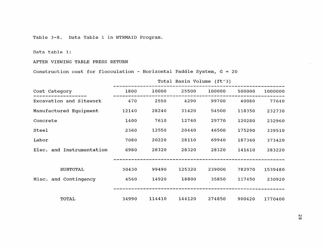
Table 3-8. Data Table 1 in WTRMAID Program.

Data table 1:

AFTER VIEWING TABLE PRESS RETURN

construction cost for flocculation - Horizontal Paddle System, G 20

Total Basin Volume (ft A 3)

Cost Category 1800 10000 25500 100000

Excavation and sitework 470 2550 4290 99700

Manufactured Equipment 12140 28240 31420 54500

Concrete 1400 7610 12740 29770

Steel 2360 12550 20440 46500

Labor 7080 20220 28110 69940

Elec. and Instrumentation 6980 28320 28320 28320

SUBTOTAL 30430 99490 125320 239000

Misc. and contingency 4560 14920 18800 35850

TOTAL 34990 114410 144120 274850

500000

40080

118350

120280

175290

187360

141610

782970

117450

900420

1000000

77640

232730

232960

339510

373420

283220

1539480

230920

1770400

I\)

00

1 A

611

1000

8192

DY ED A D

E C

B

[8J G

A- INTRODUCTORY MESSAGE B - INPUT SECTIONS C - HELP MESSAGES D - CARDS E - MACRO/MENUS F - DISKETTE MESSAGES

rl

G - PRINT FILE ~4ANIPULATlm·~ H - PRIt~T FILE MANIPULATIOt,~

Figure 3-2. Modified Iterative Measurement Test

29

1\/

30

can be a difficult task since an individual is not able to

view the possible process selections and their abbreviations

when inputting data in this section. with the WTRMAID

program the user is given this information.

The WTRMAID program is more flexible, allowing the user

to move freely to any section at any time. If a person is

inputting data in the rapid mixing process section and

remembers that the chemical cost for the coagulant was not

updated, that person can move to the chemical cost section,

update the cost of the coagulant, and then return to the

rapid mixing input section. It is recognized that both

programs could be rewritten to exactly copy the other in the

form of logical sequence of data input and output, except in

the area of data base knowledge.

Lotus 123 provides the powerful ability to have the

best available technology located right within the spread­

sheet in the form of tables, equations, graphs, and even

figures and maps can be duplicated using the Lotus 123 graph

commands. All calculations can be documented to allow for

convenient checking by anyone trying to understand the

program.

The macro in the WTRMAID program, while producing the

same output as the WATERMAID program, requires much less

programming. The rapid mix process requires seven pages of

BASIC programming while less than a page of macro program­

ming accomplishes the same result. Less programming will

31

make eventual improvements and modifications of the program

a relatively easy matter.

CHAPTER IV PRE- AND POSTPROCESSORS FOR

A HYDRAULIC PIPE NETWORK ANALYSIS MODEL

Introduction

Wood (1980) has developed a popular program in FORTRAN

IV, G level, for computer analysis of flow in pipe networks.

Wood's model was chosen because it is the most widely used

program to assist in the analysis of surcharged flow in pipe

networks and as a tool for future capacity expansion of the

network (Cesario, 1984).

Much of the time involved with modeling, such as with

Wood's model, is spent in handling the required data prior

to data input and in handling the output. Any means of

streamlining the data handling process eases the time and

complexities involved with model use.

Several methods exist to enter input data into Wood's

model. An interactive input data program (INPUTF), provided

within Wood's program, can be used for the initial input of

data. Word processors like Word Perfect or Word Star can be

used to make changes but may be complicated by the addition

of hidden characters which can cause errors during program

execution. Also, changes can be made using the line editor

(EDLIN) which is provided on the DOS disk for the IBM

personal computer and similar computers, or the IBM PC

Personal Editor.

32

33

The major drawback with the INPUTF program is the time

required to input data, and the INPUTF program will only

compile the data which are input during the initial use of

the INPUTF program. If all of the data cannot be entered

during the initial data input session, then the user is not

able to reenter the INPUTF program to complete the input of

data. There is a method to use the INPUTF program to

partially enter the entire data set but the remaining data

entered at a later time, or corrections, would have to be

entered using another editing method.

Lotus 123 Pre- and Postprocessors

A Lotus 123 program was written to increase the speed

at which data can be entered for application with Wood's

hydraulic network program, and to create a program which

does not require all data to be input during the initial

data input session. This program preprocesses the hydraulic

network data into a format which is recognized by Wood's

hydraulic network analysis program. The program is quick

and does not require all data to be input at one time.

Previous work has been conducted by Miles and Heaney (1986)

in producing slmilar data handling processors for a storm

water management model.

Lotus 123 can also be used as a postprocessor. A

postprocessing program was written which receives the output

file from Wood's program and formats the data into a Lotus

123 spreadsheet. Once the data are formatted, a multitude

of data management functions can be used to analyze the

output data.

computer Analysis of Flow in Pipe Networks

34

Pipe network equations for steady state analysis have

been expressed through loop or nodal equations. Wood's

program uses loop equations which have demonstrated superior

convergence (Wood, 1980; Viessman and Hammer, 1985). Loop

equations express mass continuity and conservation of energy

for the discharge in each pipe section. The number of pipe

sections is determined from the following:

p = j + I + f - 1 (4. 1)

where

p = number of pipe sections,

j number of junction nodes,

I = number of primary loops, and

f = number of fixed grade nodes.

A junction node is described as a point where either

two or more pipes meet, flow is gained or lost from the

system, or a change in pipe diameter occurs. A fixed grade

node is any point where the hydraulic grade line is known

which is usually a connection to a storage tank or reser­

voir, or a known pressure at any source or discharge point.

Primary loops are defined as a closed pipe circuit where all

pipes are open. As an example, Figure 4-1 details a

hydraulic pipe network with 7 pipes, 4 junction nodes,

3000

8192

BB cc

A 1O[JJ

103m

E I

A - COMPLETED FILE B - ~1ACRo/rT1ENU C - FILE IMPORT AREA D - DISKETTE MESSAGE

C

E - INTRODUCTORY MESSAGE

Figure 4-1. water Distribution Network

35

IV

36

2 fixed grade notes, and 2 primary loops (Viessman and

Hammer, 1985).

Mass continuity and Energy Conservation Eguations

Equation 1 also provides the basis for a set of

hydraulic equations which described the pipe network. A set

of p equations can be formed, which include j mass con-

tinuity equations, 1 loop energy conservation equations, and

f - 1 fixed grade node energy conservation equations.

Continuity of mass is expressed for each junction node as:

rQin - LQout = Qe (j equations) (4.2)

where

Qe = the external inflow or demand,

Qin = inflow, and

Qout = demand

Energy conservation at each primary loop is expressed as

follows:

where

(1 equations) (4.3)

hl = energy loss in each pipe (including minor loss) and

Ep = energy input into the fluid by a pump.

For f fixed grade nodes, f - 1 conservation of energy

equations can be written for paths of pipe sections between

each set of two different fixed nodes as follows:

(f-1 equations) (4.4)

where

37

dE = the difference in total grade between the two fixed grade nodes.

As stated above, the energy loss, hl' includes minor

losses. Therefore the equation for the energy loss in the

pipe is:

(4.5)

where

hlP = the line loss in the pipe, and

h l = = the minor loss in the pipe.

The line loss expressed in terms of the flow rate is

given by:

where

(4.6)

Kp = the pipe line constant which is a function of the length, diameter, and roughness or friction factor of the pipe,

Q = the flow rate, and

n = an exponent.

The values of Kp and n depend on the energy loss expression

used for the analysis. For the Hazen Williams equation:

where

(4.7)

x = a constant which depends on the units used and has a value of 4.73 for english units and 10.69 for 8I units,

L = pipe length,

38

c = the roughness coefficient, and

D = pipe diameter,

and the value of n in equation 4.6 is 1.852.

The equation for the minor loss within a pipe section

is:

(4.8)

where K~ is a function of the sum of the minor loss coeffi-

cients for the fittings in the pipe section and the pipe

diameter as follows:

(4.9)

where

m = the sum of the minor loss coefficients for the fittings in the pipe section.

The energy input to a fluid by a pump, Ep , described

by the useful power or by operating data as follows:

(4.10)

and

Ep = A + B*Q + C*Q2

respectively where A, Band C are constant. The term Z is a

function of the useful power of the pump and the specific

gravity of the fluid and is:

Z = 8.814*Pu /S (English units) (4.11)

or

where

z = .10197*P~/5 (5I units)

P~ = the useful power of the pump, and

5 = the specific gravity of the liquid.

utilizing equations 4.5 through 4.11, the energy

equations (equations 4.3 and 4.4) can be rewritten as:

(4.12)

and

39

The continuity of mass equation (equation 4.2) and

conservation of energy equations (equations 4.3 and 4.4)

form a set of P simultaneous equations in terms of unknown

flow rates which are called the loop equations. There is no

direct solution of these equations since the energy equa­

tions are nonlinear. The most reliable and efficient

algorithm, the linear method, was chosen for Wood's program

(Viessman & Hammer, 1985).

The Linear Method

The linear method involves linearizing the energy equa­

tions in terms of an approximate flow rate in each pipe.

The algorithm makes use of gradient methods to handle the

non-linear flow rate, Q, terms in the energy equations

(equation 4.12). The right hand side of equation 4.12 is

the grade difference across a pipe section carrying a flow

rate Q. This can be expressed as a function of Q as follows:

40

f(Q) (4.13 )

or

The grade difference in a pipe section based on Q = Ql is:

( 4 . 14 )

or

and the gradient evaluated at Q = Ql is:

G · CL. (4.15 )

or

The non-linear energy equations (equation 4.12) are now

linearized by taking the derivative of the variables in

equation 4.14 or 4.15 with respect to the flow rate and

evaluating them at Q = Ql using the following approximation:

(4.16)

When this relationship is applied to the energy equa-

tions (equation 4.12) the following linearized equation

results:

(4.17)

or

41

Equation 4.17 is now used to formulate the 1 + f - 1 energy

equations in addition to the j continuity equations which

form the set of p simultaneous equations.

Routine matrix procedures are used to solve the set of

p simultaneous equations after an arbitrary flow rate for

each pipe is picked. New flow rates are determined which

are then used for the second trial. Trials are repeated

until the change in flow from one trial to the next is

negligible. Since the procedure simult~neously solves for

the flow in each pipe, convergence is rapid and usually only

requires from four to eight trials.

Solution of the Linear Method Using Lotus 123

Table 4-1 (Viessman & Hammer, 1985) lists the physical

characteristics for the same hydraulic network shown in

Figure 4-1. The values for Kp , K= and Z are demonstrated in

Table 4-2 for each pipe section, using equations 4.7, 4.9,

and 4.11 respectively. In Table 4-3, the values for Q~, G~,

and H~ are determined for each pipe. The initial value for

Q is calculated from an assumed pipe velocity of 1 foot per

second. Table 4-4 demonstrates how equation 4.17 is

determined for each conservation of energy equation, loop 1,

loop 2, and path AB.

42

Table 4-1. Physical Characteristics for Pipes in Figure 4-1-

Length Diameter Area Roughness

L D A Coef

Pipe (ft) (in) (ftA2) C

1 200 6 0.785 130

2 150 4 0.349 130

3 150 3 0.196 130

4 155 3 0.196 130

5 160 6 0.785 130

6 200 4 0.349 130

7 250 3 0.196 130

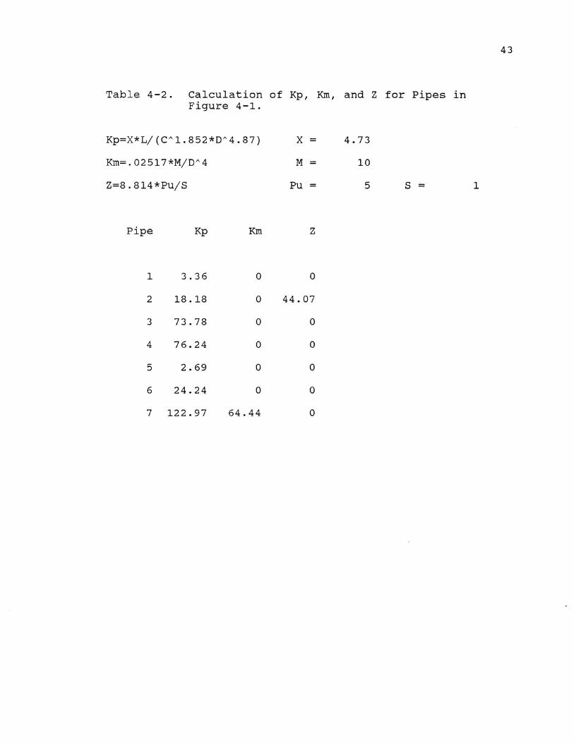
Table 4-2. Calculation of Kp, KID, and Z for Pipes in Figure 4-1.

Kp=X*L/(C A 1.852*DA 4.87)

Km=.02517*M/D A 4

Z=8.814*Pu/S

Pipe Kp Km

1 3.36 0

2 18.18 0

3 73.78 0

4 76.24 0

5 2.69 0

6 24.24 0

7 122.97 64.44

x = 4.73

M = 10

Pu = 5 S =

Z

0

44.07

0

0

0

0

0

43

1

Table 4-3. Calculation of Qi, Hi, and Gi for Pipes in Figure 4-1.

44

Qi is based on a velocity of 1 ft/sec, Q=V*A, V=l therefore

Q=A

Gi = 1.852*KpA.852 + 2*Km*Qi + Z/Qi A2

Pipe Qi Hi Gi

1 0.785 2.151 5.072

2 0.349 -123.7 375.415

3 0.196 3.620 34.140

4 0.196 3.740 35.278

5 0.785 1. 721 4.057

6 0.349 3.451 18.308

7 0.196 8.517 82.204

Table 4-4. Calculation of summation of Gi*Qi.

sum Gi*Qi = sum (Gi*Qi - Hi) + dE

Pipe No. and

Sign Gi Qi Gi*Qi Hi

Loop 1 2+ 375.415 * 0.349 = 131. 044 123.663 6+ 18.308 * 0.349 = 6.391 -3.451 5- 4.057 * 0.785 = -3.187 1. 721

----------------134.248 121.933

sum Gi*Qi = sum (Gi*Qi - Hi) + dE =

Loop 2 6- 18.308 * 0.349 = -6.391 3.451 3+ 34.140 * 0.196 = 6.703 -3.620 4- 35.278 * 0.196 = -6.927 3.740

-----------------6.614 3.571

sum Gi*Qi = sum (Gi*Qi - Hi) + dE =

PATH AB 1+ 5.072 * 0.785 = 3.983 -2.151 2+ 375.415 * 0.349 = 131. 044 123.66 3+ 34.140 * 0.196 = 6.703 -3.620 7+ 82.204 * 0.196 = 16.141 -8.52

----------------157.871 109.376

sum Gi*Qi = sum (Gi*Qi - Hi) + dE =

dE

0

256.181

0

-3.043

25.38

292.627

~ U1

Solving a Set of Simultaneous Equations Usinq Matrix Technigues

A matrix (Table 4-5) is now developed so that the

46

seven equations (p=j+1+f-1 or 4+2+2-1=7) and seven unknowns

(Q1, Q2, ... , Q7) can be solved simultaneously. There

are j = 4 mass continuity equations (equation 4.2).

Anequation is included for each junction node. For example,

the mass balance for junction node 4 is Q4 - Q5 - Q6 = o.

Notice that the right hand side (RRS) of this equation is

the external inflow or demand, which at this junction node

is always equal to zero. The energy conservation equation

for loop 2 (equation 4.17) is 34.14*Q3 - 35.28*Q4) -

18.31*Q6 = -3.04. The negative sign indicates that the flow

in pipe four is moving in a counter clockwise direction.

The right hand side of the equation is equal to the value

determined in Table 4-4.

The seven by seven matrix is solved in Lotus by

inverting the left hand side (LHS), and post-multiplying

this inverse by the right hand side vector to determine the

new Q values. The matrix procedures are also shown in Table

4-5. The new values for Q1 through Q7 are now used to

update Table 4-3 and the entire process is repeated to

determine another set of Q values. The iterative process

stops when the change in Q values is within an established

tolerance. Tables 4-6, 4-7, 4-8, and 4-9 show the second,

third, fourth, and fifth iterations for this hydraulic

network. The final Q values are Q1=1.73, Q2=1.37, Q3=0.37,

Q4=0.36, Q5=0.001, and Q7=0.132. Table 4-10 is the output

Table 4-5. Matrix for Solving Simultaneous Equations.

LHS Q1 Q2 Q3 Q4 Q5 Q6 Q7 RHS

PATH AB 5.07 375.41 34.14 0.00 0.00 0.00 82.20 292.63 LOOP 1 0.00 375.41 0.00 0.00 -4.06 18.31 0.00 256.18 LOOP 2 0.00 0.00 34.14 -35.28 0.00 -18.31 0.00 -3.04 JUNe 1 -1. 00 1. 00 0.00 0.00 1. 00 0.00 0.00 0.00 JUNe 2 0.00 -1. 00 1. 00 0.00 0.00 1. 00 0.00 -1.00 JUNe 3 0.00 0.00 -1. 00 -1.00 0.00 0.00 1.00 -0.60 JUNe 4 0.00 0.00 0.00 1. 00 .-1. 00 -1. 00 0.00 0.00

LHS"-l RHS 0.01 -0.01 -0.01 -0.95 -0.86 -0.73 -0.92 292.63 0.00 0.00 0.00 0.00 -0.04 -0.02 -0.01 256.18 0.00 0.00 0.01 0.02 0.26 -0.30 0.03 -3.04 0.01 -0.01 -0.01 0.03 -0.11 -0.43 0.05 * 0.00 0.01 -0.01 -0.01 0.04 -0.81 -0.71 -0.91 -1.00 0.00 0.01 -0.01 -0.02 0.70 0.28 -0.04 -0.60 0.01 -0.01 -0.01 0.05 0.14 0.27 0.08 0.00

Q 1.7051 1 0.7162 2 0.1896 3

= new Q values = 0.5155 4 0.9890 5

-0.4735 6 0.1051 7

LHS RHS 292.63 292.63 256.18 256.18 -3.04 -3.04

0.00 = 0.00 -1. 00 -1.00 -0.60 -0.60

*" 0.00 0.00 ~

Table 4-6. Second Iteration of Linear Method.

Qi is based on a velocity of 1 ft/sec, Q=V*A, V=l therefore Q=A Gi = 1.852*KpA.852 + 2*Km*Qi + Z/Qi A2 Hi = Kp*Qi A1.852 + Km*Qi A2 - Z/Qi

Qi 1 1. 7051

2 0.7162 3 0.1896 4 0.5155 5 0.9890 6 0.4735 7 0.1051

Hi Gi 9.039 9.817

-51. 7 Ill. 252 3.394 33.144

22.348 80.290 2.637 4.938 6.069 23.738 2.610 46.969

sum Gi*Qi = sum (Gi*Qi - Hi) + dE

Loop 1

Pipe No. and

Sign Gi

2+ 111.252 6+ 23.738 5- 4.938

* * *

Qi

0.716 0.473 0.989

= = =

Gi*Qi Hi

79.676 51.740 11. 239 -6.069 -4.883 2.637

86.0316 48.3082

sum Gi*Qi = sum (Gi*Qi - Hi) + dE =

Loop 2 6- 23.738 * 0.473 = -11. 239 6.069 3+ 33.144 * 0.190 = 6.286 -3.394 4- 80.290 * 0.515 = -41.389 22.348

-----------------46.343 25.023

sum Gi*Qi = sum (Gi*Qi - Hi) + dE =

dE

o

134.339

0

-21. 320 ~ OJ

Table 4-6. continued.

PATH AB 1+ 9.817 2+ 111.252 3+ 33.144 7+ 46.969

Q1 Q2

PATH AB 9.82 111.25 LOOP 1 0.00 111. 25 LOOP 2 0.00 0.00 JUNC 1 -1.00 1. 00 JUNC 2 0.00 -1. 00 JUNC 3 0.00 0.00 JUNC 4 0.00 0.00

0.01 -0.01 0.00 0.00 0.01 0.00 0.01 0.00 0.00 0.00 0.00 -0.01 0.01 -0.02 0.00

-0.01 0.01 0.00 0.01 -0.01 0.00

* 1. 705 16.740 -9.039 * 0.716 = 79.676 51. 74 * 0.190 6.286 -3.394 * 0.105 = 4.938 -2.61

----------------107.639 36.6979

sum Gi*Qi = sum (Gi*Qi - Hi) + dE

LHS Q3 Q4 Q5 Q6 Q7

33.14 0.00 0.00 0.00 46.97 0.00 0.00 -4.94 23.74 0.00

33.14 -80.29 0.00 -23.74 0.00 0.00 0.00 1. 00 0.00 0.00 1. 00 0.00 0.00 1. 00 0.00

-1. 00 -1. 00 0.00 0.00 1. 00 0.00 1. 00 -1. 00 -1. 00 0.00

LHS"-l -0.89 -0.73 -0.51 -0.85

0.01 -0.14 -0.07 -0.02 0.06 0.31 -0.31 0.09 0.04 -0.04 -0.20 0.07 * 0.09 -0.58 -0.44 -0.83

-0.05 0.55 0.24 -0.10 0.11 0.27 0.49 0.15

25.38

169.717

RHS

169.72 134.34 -21. 32

0.00 -1. 00 -0.60

0.00

RHS 169.72 134.34 -21.32

0.00 -1. 00 -0.60

0.00

~ I.D

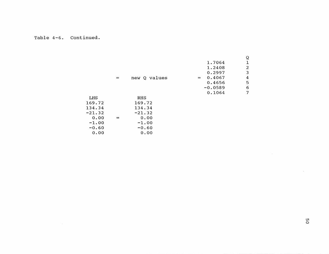
Table 4-6. continued.

LHS 169.72 134.34 -21. 32

0.00 -1.00 -0.60

0.00

=

=

new Q values

RHS 169.72 134.34 -21. 32

0.00 -1.00 -0.60

0.00

1.7064 1. 2408 0.2997 0.4067 0.4656

-0.0589 0.1064

Q 1 2 3 4 5 6 7

Ul o

Table 4-7. Third Iteration of Linear Method.

Qi is based on a velocity of 1 ft/sec, Q=V*A, V=1 therefore Q=A Gi 1.852*Kp~.852 + 2*Km*Qi + Z/Qi~2 Hi = Kp*Qi A 1.852 + Kro*Qi A 2 - Z/Qi

Qi Hi Gi 1 1. 7064 9.051 9.823 2 1. 2408 -8.4 69.081 3 0.2997 7.921 48.947 4 0.4067 14.405 65.602 5 0.4656 0.653 2.599 6 0.0589 0.128 4.021 7 0.1064 2.667 47.454

sum Gi*Qi = sum (Gi*Qi - Hi) + dE

Pipe No. and

Sign Gi Qi Gi*Qi Hi

Loop 1 2+ 69.081 * 1.241 = 85.714 8.415 6+ 4.021 * 0.059 = 0.237 -0.128 5- 2.599 * 0.466 = -1. 210 0.653

----------------84.7409 8.94027

sum Gi*Qi = sum (Gi*Qi - Hi) + dE =

Loop 2 6- 4.021 * 0.059 = -0.237 0.128 3+ 48.947 * 0.300 = 14.669 -7.921 4- 65.602 * 0.407 = -26.678 14.405

-----------------12.246 6.612

sum Gi*Qi = sum (Gi*Qi - Hi) + dE =

dE

0

93.6812

0

-5.634 Ul I-'

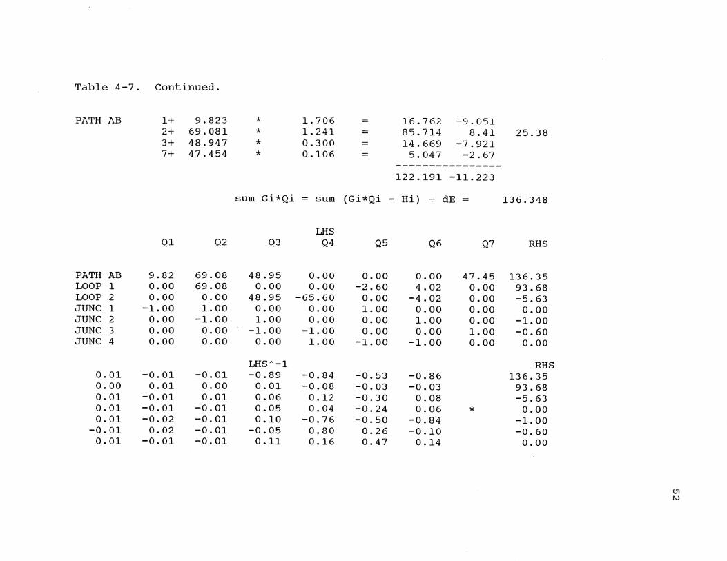
Table 4-7. continued.

PATH AB 1+ 9.823 2+ 69.081 3+ 48.947 7+ 47.454

Q1 Q2

PATH AB 9.82 69.08 LOOP 1 0.00 69.08 LOOP 2 0.00 0.00 JUNC 1 -1. 00 1. 00 JUNC 2 0.00 -1. 00 JUNC 3 0.00 0.00 JUNC 4 0.00 0.00

0.01 -0.01 -0.01 0.00 0.01 0.00 0.01 -0.01 0.01 0.01 -0.01 -0.01 0.01 -0.02 -0.01

-0.01 0.02 -0.01 0.01 -0.01 -0.01

* 1.706 16.762 -9.051 * 1. 241 = 85.714 8.41 * 0.300 = 14.669 -7.921 * 0.106 5.047 -2.67

----------------122.191 -11.223

sum Gi*Qi = sum (Gi*Qi - Hi) + dE =

LHS Q3 Q4 Q5 Q6 Q7

48.95 0.00 0.00 0.00 47.45 0.00 0.00 -2.60 4.02 0.00

48.95 -65.60 0.00 -4.02 0.00 0.00 0.00 1. 00 0.00 0.00 1. 00 0.00 0.00 1. 00 0.00

-1. 00 -1. 00 0.00 0.00 1. 00 0.00 1. 00 -1. 00 -1.00 0.00

LHS"-l -0.89 -0.84 -0.53 -0.86

0.01 -0.08 -0.03 -0.03 0.06 0.12 -0.30 0.08 0.05 0.04 -0.24 0.06 * 0.10 -0.76 -0.50 -0.84

-0.05 0.80 0.26 -0.10 0.11 0.16 0.47 0.14

25.38

136.348

RHS

136.35 93.68 -5.63

0.00 -1. 00 -0.60

0.00

RHS 136.35

93.68 -5.63

0.00 -1. 00 -0.60

0.00

Ul [\)

Table 4-7. continued.

= new Q values

LHS RHS 136.35 136.35

93.68 93.68 -5.63 -5.63

0.00 = 0.00 -1.00 -1. 00 -0.60 -0.60

0.00 0.00

1. 7358 1. 3700 0.3721 0.3637 0.3658

-0.0021 0.1358

Q 1 2 3 4 5 6 7

U1 W

Table 4-8. Fourth Iteration of Linear Method.

Qi is based on a velocity of 1 ft/sec, Q=V*A, V=1 therefore Q=A Gi 1.852*KpA.852 + 2*Km*Qi + Z/Qi A 2 Hi = Kp*Qi A l.852 + Km*Qi A 2 - Z/Qi

Qi Hi Gi

1 1. 7358 9.342 9.967 2 1.3700 0.4 67.499 3 0.3721 11. 827 58.861 4 0.3637 11. 711 59.642 5 0.3658 0.418 2.116 6 0.0021 0.000 0.238 7 0.1358 4.234 59.052

sum Gi*Qi = sum (Gi*Qi - Hi) + dE

Pipe No. and

Sign Gi Qi Gi*Qi Hi

Loop 1 2+ 67.499 * 1. 370 = 92.473 -0.393 6+ 0.238 * 0.002 0.001 0.000 5- 2.116 * 0.366 = -0.774 0.418

91.6990 0.02421

sum Gi*Qi = sum (Gi*Qi - Hi) + dE =

dE

0

91. 7232

(Jl

of:>.

Table 4-8. continued.

Loop 2 6- 0.238 3+ 58.861 4- 59.642

PATH AB 1+ 9.967 2+ 67.499 3+ 58.861 7+ 59.052

Q1 Q2

PATH AB 9.97 67.50 LOOP 1 0.00 67.50 LOOP 2 0.00 0.00 JUNC 1 -1. 00 1. 00 JUNC 2 0.00 -1. 00 JUNC 3 0.00 0.00 JUNC 4 0.00 0.00

* 0.002 -0.001 0.000 * 0.372 = 21. 903 -11. 827 * 0.364 = -21. 689 11. 711

----------------0.213 -0.115

sum Gi*Qi = sum (Gi*Qi - Hi) + dE =

* 1. 736 = 17.301 -9.342 * 1. 370 = 92.473 -0.39 * 0.372 = 21. 903 -11. 827 * 0.136 = 8.018 -4.23

----------------139.694 -25.796

sum Gi*Qi sum (Gi*Qi - Hi) + dE =

LHS Q3 Q4 Q5 Q6 Q7

58.86 0.00 0.00 0.00 59.05 0.00 0.00 -2.12 0.24 0.00

58.86 -59.64 0.00 -0.24 0.00 0.00 0.00 1. 00 0.00 0.00 1. 00 0.00 0.00 1. 00 0.00

-1. 00 -1.00 0.00 0.00 1. 00 0.00 1.00 -1.00 -1. 00 0.00

0

0.098

25.38

139.278

RHS

139.28 91. 72

0.10 0.00

-1. 00 -0.60 0.00

01 01

Table 4-8. continued.

LHS"-l 0.01 -0.01 0.00 -0.90 0.00 0.01 0.00 0.00 0.00 0.00 0.01 0.05 0.00 0.00 -0.01 0.05 0.01 -0.02 0.00 0.10 0.00 0.02 -0.01 -0.05 0.01 -0.01 0.00 0.10

LHS 139.28

91. 72 0.10 0.00

-1.00 -0.60

0.00

-0.88 -0.59 -0.03 -0.02

0.06 -0.29 0.06 -0.29

-0.85 -0.57 0.91 0.28 0.12 0.41

new Q values

RHS 139.28

91. 72 0.10 0.00

-1. 00 -0.60

0.00

-0.88 -0.03

0.06 0.06

-0.85 -0.09

0.12

*

1.7320 1.3702 0.3692

= 0.3627 0.3618 0.0010 0.1320

RHS 139.28

91. 72 0.10 0.00

-1. 00 -0.60

0.00

Q 1 2 3 4 5 6 7

1Jl 0'1

Table 4-9. Fifth and Final Iteration of Linear Method.

Qi is based on a velocity of 1 ft/sec, Q=V*A, V=l therefore Q=A Gi = 1.852*KpA.852 + 2*Km*Qi + Z/Qi A2 Hi = Kp*Qi A1.852 + Km*Qi A2 - Z/Qi

Qi

1 1. 7320 2 1. 3702 3 0.3692 4 0.3627 5 0.3618 6 0.0010 7 0.1320

Hi

9.304 0.4

11.657 11.657

0.409 0.000 4.013

Gi

9.949 67.497 58.471 59.514

2.096 0.123

57.569

sum Gi*Qi = sum (Gi*Qi - Hi) + dE

Loop 1

Pipe No. and

Sign

2+ 6+ 5-

Gi

67.497 0.123 2.096

* * *

Qi

1. 370 0.001 0.362

=

= =

Gi*Qi

92.486 0.000

-0.758

Hi

-0.409 0.000 0.409

91. 7281 -0.0000

sum Gi*Qi = sum (Gi*Qi - Hi) + dE =

dE

o

91. 7280

Ul -....J

Table 4-9. continued.

Loop 2 6- 0.123 3+ 58.471 4- 59.514

PATH AB 1+ 9.949 2+ 67.497 3+ 58.471 7+ 57.569

Q1 Q2

PATH AB 9.95 67.50 LOOP 1 0.00 67.50 LOOP 2 0.00 0.00 JUNC 1 -1. 00 1. 00 JUNC 2 0.00 -1. 00 JUNe 3 0.00 0.00 JUNC 4 0.00 0.00

* 0.001 = 0.000 0.000 * 0.369 = 21.589 -11.657 * 0.363 = -21. 589 11. 657

----------------0.001 0.000

sum Gi*Qi = sum (Gi*Qi Hi) + dE =

* 1. 732 = 17.231 -9.304 * 1. 370 92.486 -0.41 * 0.369 = 21. 589 -11. 657 * 0.132 7.598 -4.01

----------------138.904 -25.383

sum Gi*Qi sum (Gi*Qi - Hi) + dE =

LHS Q3 Q4 Q5 Q6 Q7

58.47 0.00 0.00 0.00 57.57 0.00 0.00 -2.10 0.12 0.00

58.47 -59.51 0.00 -0.12 0.00 0.00 0.00 1. 00 0.00 0.00 1. 00 0.00 0.00 1. 00 0.00

-1. 00 -1. 00 0.00 0.00 1. 00 0.00 1. 00 -1. 00 -1.00 0.00

0

0.000

25.38

138.900

RHS

138.90 91. 73

0.00 0.00

-1. 00 -0.60

0.00

Ul 00

Table 4-9. Continued.

LHSA-1 0.01 -0.01 -0.01 -0.90 -0.88 -0.58 0.00 0.01 0.00 0.00 -0.03 -0.02 0.01 0.00 0.01 0.05 0.06 -0.29 0.01 0.00 -0.01 0.05 0.06 -0.29 0.,01 -0.02 0.00 0.10 -0.85 -0.56 0.00 0.02 -0.01 -0.05 0.9l 0.27 0.01 -0.01 -0.01 0.10 0.12 0.42

= new Q values

LHS RHS 138.90 138.90

91. 73 91. 73 0.00 0.00 0.00 = 0.00

-1.00 -1.00 -0.60 -0.60

0.00 0.00

-0.88 -0.03

0.06 0.06 * -0.85

-0.09 0.12

1. 7319 1. 3702 0.3692

= 0.3627 0.3617 0.0010 0.1319

RHS 138.90

91. 73 0.00 0.00

-1. 00 -0.60

0.00

Q 1 2 3 4 5 6 7

Ul \0

Table 4-10. Wood's Model Solution to Pipe Network in Figure 4-1.

FLOWRATE IS EXPRESSED IN CFS AND PRESSURE IN PSIG

A SUMMARY OF THE ORIGINAL DATA FOLLOWS

PIPE NO. NODE NOS. LENGTH (FEET)

200.0 150.0

DIAMETER (INCHES)

6.0 4.0

1 0 1 2 1 2

THERE IS A PUMP IN 3 2 3 4 4 3 5 1 4 6 2 4 7 3 0

LINE 2 WITH 150.0 155.0 160.0 200.0 250.0

USEFUL 3.0 3.0 6.0 4.0 3.0

ROUGHNESS

130.0 130.0

POWER = 130.0 130.0 130.0 130.0 130.0

MINOR LOSS K

.00

.00 5.00

.00

.00

.00

.00 10.00

JUNCTION NUMBER DEMAND ELEVATION CONNECTING PIPES 1 .00 90.00 1 2 5 2 1. 00 100.00 2 3 6 3 .60 90.00 3 4 7 4 .00 80.00 4 5 6

OUTPUT SELECTION: ALL RESULTS ARE OUTPUT EACH PERIOD

THIS SYSTEM HAS 7 PIPES WITH 4 JUNCTIONS , 2 LOOPS AND

FIXED GRADE

215.38

190.00

2 FGNS

THE RESULTS ARE OBTAINED AFTER 5 TRIALS WITH AN ACCURACY = .00062

FILL THIS SECTION WITH ANY INPUT YOU DESIRE TO DESCRIBE YOUR HYDRAULIC NETWORK PROGRAM

0'1 o

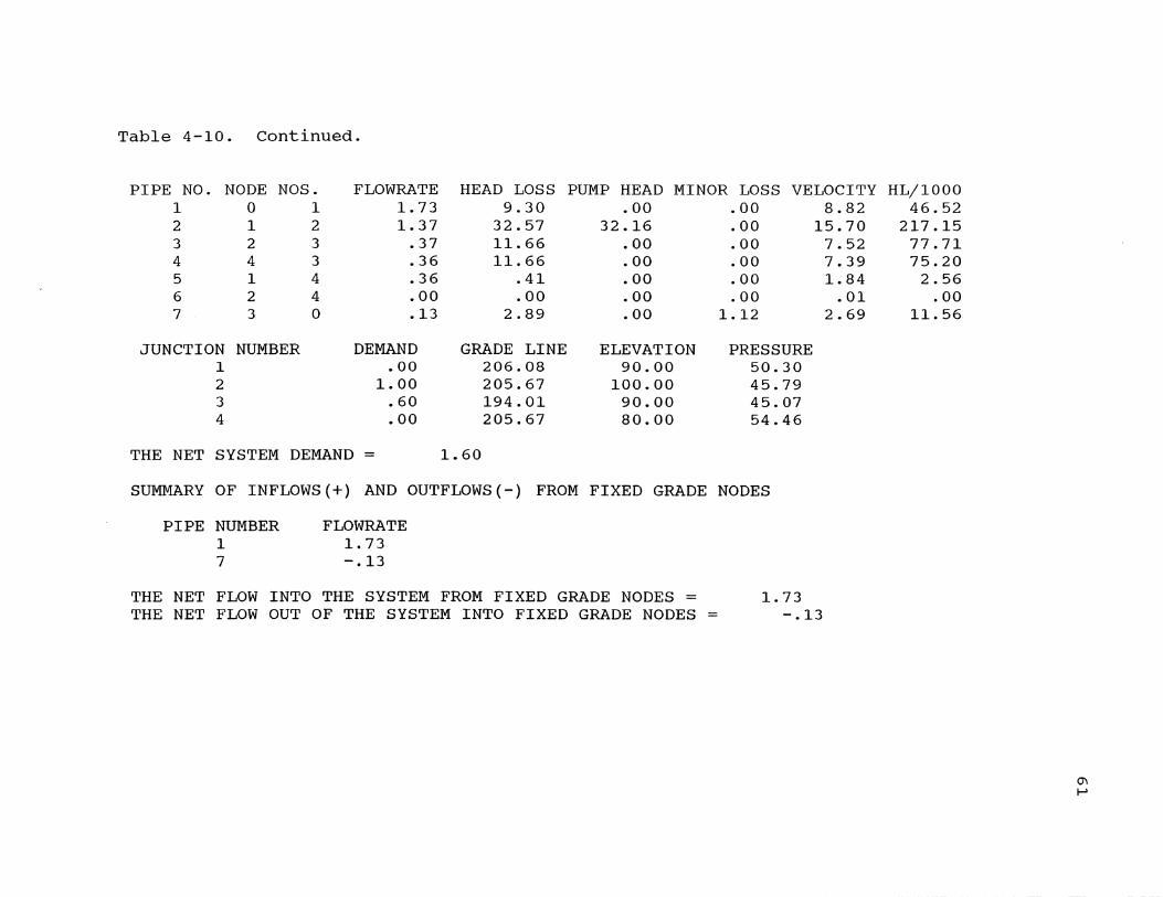
Table 4-10. continued.

PIPE NO. NODE NOS. FLOWRATE HEAD LOSS PUMP HEAD MINOR LOSS VELOCITY HL/1000 1 0 1 2 1 2 3 2 3 4 4 3 5 1 4 6 2 4 7 3 0

JUNCTION NUMBER 1 2 3 4

1. 73 1. 37

.37

.36

.36

.00

.13

DEMAND .00

1. 00 .60 .00

9.30 32.57 11. 66 11. 66

.41

.00 2.89

GRADE LINE 206.08 205.67 194.01 205.67

THE NET SYSTEM DEMAND = 1.60

.00 32.16

.00

.00

.00

.00

.00

ELEVATION 90.00

100.00 90.00 80.00

.00

.00

.00

.00

.00

.00 1.12

PRESSURE 50.30 45.79 45.07 54.46

8.82 15.70

7.52 7.39 1.84

.01 2.69

SUMMARY OF INFLOWS(+) AND OUTFLOWS(-) FROM FIXED GRADE NODES

PIPE NUMBER 1 7

FLOWRATE 1. 73 -.13

THE NET FLOW INTO THE SYSTEM FROM FIXED GRADE NODES = THE NET FLOW OUT OF THE SYSTEM INTO FIXED GRADE NODES =

1. 73 -.13

46.52 217.15 77.71 75.20 2.56

.00 11. 56

0"1 I-'

62

file from Wood's program for the same network showing the

solution of the same flow rate for each pipe. The solutions

are the same.

Additional Features in Wood's Model

The program features an extended period simulation. A

steady state analysis is carried out as outlined above for a

specific set of conditions and time periods. The computed

flows into and out of the storage tanks are then used to

project the change in tank water levels over the next time

interval. A new steady state solution is then carried out

with the new water levels.

Analysis of a surcharged storm sewer systems is

possible with the program. In one application the flooded

inlets to the storm sewer system are modeled as storage

tanks. The amount of water entering the inlet detention

tank can be determined from the runoff hydrograph. The

program determines how high the water rises at the inlet

detention basins and how the sewer system will handle the

flow. The program runs until the inlet pools have emptied.

In a second application, the program can determine the

height to which water will rise in manholes, when the

manholes are input as junction nodes.

Lotus 123 Preprocessor

The Lotus 123 spreadsheet which contains Wood's

Hydraulic Network preprocessor is listed as file

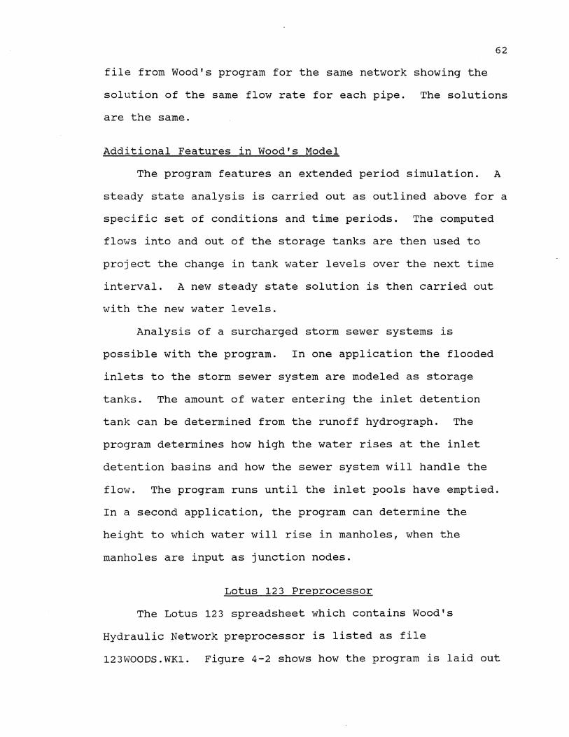
123WOODS.WK1. Figure 4-2 shows how the program is laid out

1

421

A J Y AJ AS BB BL IA IV A

C D E F G H

B

J

A ~ INTRODUCTORY MESSAGE B - SECTIONS C - MACRO D - LOG GRAPH E - FLOC PROCESS F - RAPID t~IXING PROCESS G - DATA TABLES H - CONTAMINANT SECTION I - OUTPUT AREA J - PROCESS SORTING AREA

I

63

Figure 4-2. Spreadsheet Diagram of Wood's Model Preprocessor

64

within the spreadsheet. A separate area within the spread­

sheet contains the input sections, help messages, cards,

macros and menus, diskette messages, and two areas for

manipulation of the cards.

At this time the preprocessor will accept a network

containing up to 100 pipes, 100 junction nodes, 100 pumps,

and 32 pressure regulating valves. The program can be

easily expanded to 1000 pipes, 1000 junction nodes, and 1000

pumps which are the maximum inputs for Wood's program.

The Lotus 123 preprocessor spreadsheet is menu driven.

Pressing the alt and M keys at the same time will activate

the menu at the top of the screen. The first command listed

is SECTIONS. If return is pressed while SECTIONS is

highlighted a new menu will appear listing each section.

Pressing return at a particular highlighted section will

cause that section to appear on the screen.

The sections are where data are input. Blank forms are

provided with Wood's program for collecting input data. The

sections within the spreadsheet are designed to look as much

like these forms as possible. This is done so that persons

already using Wood's program would be familiar with the

sections in the Lotus 123 preprocessor. Appendix G includes

a copy of each section where data can be input.

65

Spreadsheet Protection

The spreadsheet is protected so that data can only be

entered within the proper cells in each section. This is

achieved using the Lotus 123 spreadsheet, global, protec­

tion, and enable commands. Only those cells where data are

to be input are unprotected using the range and unprotect

commands. Cells where data are to be input are defined by

brackets or by columns. The cursor must be moved so that it

is located between the brackets or within the column

designated to enter data. Question marks are located within

cells where data must be entered or Wood's program will not

run due to insufficient data.

Error and Help Messages

Error and help messages are included at the data entry

locations. If a number is entered that is not within the

range of acceptable values the word ERROR will appear next

to the data entry point. This is achieved using the Lotus

123 @if function to check the data being entered. For

further assistance, a help menu is provided. Next to each

data entry location there is an alpha-numeric in the form

HI, H2, H3 .... H31. This alpha-numeric can be used in

conjunction with the help menu for additional explanation

and guidance. Pressing the alt and M keys to access the

main menu. Then move the cursor to highlight the word HELP

and press return to produce the help menu.

66

Help Menu

The help menu lists the section name. The section name

may be further divided by the help number if there are ~ore

than eight help alpha-numerics within that section (a user

written menu in Lotus 123 can only contain up to eight

commands). Highlighting a specific section within the help

menu produces a menu of all the help numbers located within

that section. Then, highlighting a particular help number

provides the desired help message. Appendix H lists the

help messages. Pressing the return key after reading the

help message returns the user to the proper data input

section.

Additional Program Features

Actually, two files are required for the preprocessor

to work. The second file is listed as BLANK.WK1. This file

contains the card section. The card section is only

combined into the 123WOODS.WK1 spreadsheet for preprocessing

purposes after all input data are entered. The card section

is removed for a very good reason; to speed up the time

required to recalculate the spreadsheet after each input is

made. Recalculation of the spreadsheet is desired so that

error messages can appear as data are entered.

Since the BLANK.WKl file is combined into the

123WOODS.WKl file the diskette cannot be write-protected.

To protect the diskette containing the 123WOODS.WK1 spread­

sheet as much as possible, diskette messages are included.

If followed, these messages will ensure that the diskette

67

containing the two preprocessing files is removed and

replaced with the user's diskette prior to saving any data.

A copy of the data which has been entered can be saved

at any time using the COPY command within the main menu.

The saved data file can then be input back into the prepro­

cessor at a future time so that more data can be entered or

changed. The command within the main menu which combines

the saved file into the preprocessor is CHANGES.

Once the input of all data is completed, the user can

instruct the preprocessor to manipulate the data into a form

which will be accepted by Wood's program. The COMPILE

command within the main menu is used for this purpose. The

input data are moved to the respective card sections. In

each card section the data are placed in the proper format

and in the proper location (Appendix I). Each piece of data

is formatted to the required number of decimal places and

the decimal point is located at the exact location required

in that row. This system is exactly that which was required

when cards were keypunched so that data could be input into

the computer. Data are formatted and the location set by

using the Lotus 123 range, format, fixed and spreadsheet,

column, set commands.

Each card section is then formatted into a print file,

using the printer and file commands. This is done to

maintain the different data format and location integrity

for each card. The print files are then imported back into

the preprocessor where the cards are manipulated into the

68

proper order. Finally, a completed print file is produced

which is in the proper format to be accepted by Wood's

program and the preprocessing program is terminated. Table

4-11 contains data for the network in Figure 4-1 which have

been preprocessed by Lotus 123. It is important to remember

that the completed file is in the format, filename.PRN

because it is a print file. Saving the file as filename.WK1

creates a file which will not be recognized by Wood's

program.

Macro

The menu system and all of the commands within the menu

are accomplished with one macro which is initiated by

pressing the alt and M keys. A copy of the macro which

includes two subroutines and nine separate menus is listed

in Appendix J. Some of the macro is hidden due to over­

lapping cells. The entire macro can be viewed on the

monitor screen by placing the cursor on each hidden cell to

view the cell contents. The macro initially introduces the

main menu. Subsequent menu selections either introduce sub

menus or a completion of the macro.

All of the available options within the system data

section are functional. These various input options are

fully explained within the help menu. The output option

data section is not functional. The output data section is

used to limit the amount of output data. Since the post­

processor is written to accept all output data from Wood's

program the output section is disregarded. Also, the

1-3 Pl

0 0 7 4 0 0 0 0 0 0.000000 0.00000 0.00000000 tJ f-J

FILL THIS SECTION (J)

WITH ANY INPUT YOU DESIRE ,j::.

TO DESCRIBE YOUR HYDRAULIC NETWORK PROGRAM I ~

0 0 1 200.00 6.00 130.00 0.00 0.00 215.38 ~

0 1 2 150.00 4.00 130.00 0.00 5.00 0.00 0 2 3 150.00 3.00 130.00 0.00 0.00 0.00 0 4 3 155.00 3.00 130.00 0.00 0.00 0.00

~ ti

0 1 4 160.00 6.00 130.00 0.00 0.00 0.00 (J) '0

0 2 4 200.00 4.00 130.00 0.00 0.00 0.00 0 3 0 250.00 3.00 130.00 10.00 0.00 190.00

ti 0 ()

0.00 90.00 1 0 0 0 0 0 0 0 0 0 (J) (Jl

1. 00 100.00 2 0 0 0 0 0 0 0 0 0 0.60 90.00 3 0 0 0 0 0 0 0 0 0

(Jl (J) 0-

0.00 80.00 4 0 0 0 0 0 0 0 0 0 H

0 :I '0

0 0 0 0 0 0 C

-2.000 rt

3 2 3 150.0 3.0 130.0 .00 0 Pl

4 4 3 155.0 3.0 130.0 .00 rt 5 1 4 160.0 6.0 130.0 .00 Pl

6 4 2 200.0 4.0 130.0 .00 7 3 0 250.0 3.0 130.0 10.00 190.

:;0 (J) Pl 0-'<:

Hl 0 ti

:8 0 0 0--(Jl

:s: 0 0-(J) f-J 0'1

1.0

extended period simulation is not included in the prepro­

cessor at this time.

Lotus 123 Postprocessor

70

The postprocessor is a much simpler program than the

preprocessor. The spreadsheet layout is demonstrated in

Figure 4-3. The postprocessor accepts the output data file

from Wood's program as an import file into Lotus 123, and

separates the data under proper headings.

As mentioned earlier, the data introduced to Wood's

program are in the format of a print file, filename.PRN.

When Wood's program is executed, by typing KYPIPEF, the

program asks the user to identify the input file. The input

file name is of the format filename.PRN. Wood's program

also asks the user to name the output file. It is important

to name the output file name with the same .PRN suffix.

Since the postprocessor is importing a file produced from

another program the file must be in the form filename.PRN to

be listed in the postprocessor for import.

The postprocessor file name is WOODS123.WK1. The

program is menu driven. The menu is accessed by pressing

the alt and M keys at the same time. There are four

options. The IMPORT command is used to import the output

file from Wood's program and manipulate the file into a

workable Lotus 123 spreadsheet. The COpy command creates

f­I~ o o z o f­o J rr: f­I? .... '-o o

r>:Jndructic, n CC(;:t f,;:::, r flc)(::(:ukJti,;:::,[', -h [J'f:wm(]1 fIOools S)~t8m5.

~E=I3=f'-=f+-=f+-=t1·· ·f .. F===t==t==+=+-+++-n====c-= = =~+-= ~ •.. ' S f--- .

r---+-~~~~r---+-~I·--+-·+-~I~r---+---+-+·~~4 ,4 ---1:--+--l:-+-+-I-Wt----t---I-+~~ t----+--+-~~ +++---i~-I- - -- ........ ..

;~-r-t-rt++~--4-~~~I~r-r~···~/+-~4~

1---r-++-t++-H+--+-t-+-!-;~.UJ1·' /:.,::,<'- - f-f-_ii2~ f--f- - ,.,

2. r--t-i-t-++-+t++--1~W"::J;'" .,: ;: .'

HY'5-~~~tmm" :~-;;;--~'--~<E:;;~~;;~:E;:"l': '1" M:1~~~i=·'--' ,_. -,. . .. It-=--+--I--"- ,., > ~ , '-' . ..

s r--t--+:::;rl' :::..';··'1+++1H--+-i.....:.r·I[] ... __ + ____ .'=:t: ... = ..

l

w4~~~mEE~=mtf=±=F-Sj St=~t=ti~Ht·tir--·~~~~~P===+=~t1~ti ~~-r~~tm----~+4~f++~---+--~L[[TI ---I-- -t-+l+t++---+-W~...I..+-H+----+---4·- f-- - - "

21-1-t-t-tt+HH--+-+-++I+~-f.~--L-,1-+-,- -.

ror.bl WI 'r,()l)M - WJ

Figure 4-3. Spreadsheet Diagram of Wood's Model postprocessor

71

72

a saved file of the spreadsheet. The HELP command returns

to the introductory message and the QUIT command terminates

the program.

Additional Features

The postprocessor diskette can be write-protected. The

user is directed to remove the diskette after the program

file is retrieved. The macro (Appendix J) involves one

menu, with the IMPORT command being the only command which

involves a macro continuation of more than one line. Again,

some of the macro is hidden due to cell overlap.

Table 4-12 shows a copy of the postprocessed output

data, seen earlier in Table 4-10, for the hydraulic pipe

network shown in Figure 4-1. The data in Table 4-10 were

imported into Lotus 123 using the file, import, and text

commands. Table 4-10 is Wood's output file. The data in

this file cannot be effectively manipulated using further

Lotus 123 commands and functions. Using the postprocessor,

the output file from Wood's program is imported using the

file, import, and numbers command. The numbers are then

placed under the proper headings so that the output data can

be recognized. The data are now in a usable format so that

they can be manipulated by Lotus commands and functions,

especially the data management commands.

The Lotus 123 data management commands can be very

useful in identifying pipes with certain characteristics.

For example, pipes which have pressures, flows, head loss,

or velocities above or below a critical value of interest to

Table 4-14. Postprocessed Output Data From WoodIs Model.

PIPE FLOW HEAD PUMP NUMBER NODE NUMBER RATE LOSS HEAD

1 0 1 1. 73 9.3 0 2 1 2 1. 37 32.57 32.16 3 2 3 0.37 11.66 0 4 4 3 0.36 11.66 0 5 1 4 0.36 0.41 0 6 2 4 0 0 0 7 3 0 0.13 2.89 0

JUNCTION GRADE ELE-NUMBER DEMAND LINE VATION PRESSURE

1 0 206.08 90 50.3 2 1 205.67 100 45.79 3 0.6 194.01 90 45.07 4 0 205.67 80 54.46

THE NET SYSTEM DEMAND = 1.6

SUMMARY OF INFLOWS(+) AND OUTFLOWS(-) FROM FIXED GRADE NODES

PIPE NUMBER

1 7

FLOW RATE

1. 73 -0.13

THE NET FLOW INTO THE SYSTEM FROM FIXED GRADE NODES = THE NET FLOW OUT OF THE SYSTEM INTO FIXED GRADE NODES =

1. 73 -0.13

MINOR LOSS

0 0 0 0 0 0

1.12

VELOCITYHL/1000

8.82 46.52 15.7 217.15

7.52 77.71 7.39 75.2 1.84 2.56 0.01 0 2.69 11.56

-.J W

the user could be separately identified. Macros can be

easily written to automate this process.

Conclusions

74

The Lotus 123 preprocessor for use with the Computer

Analysis of Flow in Pipe Networks model is an effective

tool. The preprocessor eliminates the two major problems

associated with the data input program within Wood's model.

The preprocessor allows the user to partially input data,

save the file, and return at a later time to continue data

entry. This is especially valuable when large pipe networks

are being entered for use in Wood's model.

Secondly, entering data in the preprocessor is quicker

than using Wood's input program. Data for the Kanapaha

force main network in Gainesville, Florida which contains 54

pipes, 45 nodes, and 13 pumps took one and a half hours to

enter using Wood's input program and 30 minutes to enter

using the preprocessor. Compiling the input data in wood's

input program is quicker. It takes Wood's program about a

minute versus up to eight minutes to preprocess the input

data in the preprocessor. But the overall time spent in

completing a file ready for use with Wood's model is still

much shorter using the Lotus 123 preprocessor.

The Lotus 123 preprocessor has a very definite advan­

tage in that the help system is included within the prepro­

cessing program. For an individual using Wood's model for

the first time, the preprocessor provides quick help as

opposed to having to search through the user's manual

provided with Wood's model.

The Lotus 123 postprocessor is very quick, taking

75

less than two minutes to format the output data from Wood's

model. Upon completion, the output data are in a form ready

to be further processed using the Lotus 123 data management

commands.

Most of the time spent using hydraulic network analysis

models is in the formulation of data for input into the

model and evaluation of the output data. Lotus 123 can be

effective in streamlining these processes.

CHAPTER V OPTIMAL ADJUSTMENTS IN ERRONEOUS

HYDRAULIC NETWORK FLOWS

Introduction

When modeling a hydraulic flow network it is imperative

that the actual quantity of flow in each pipe be known. The

required result is that the sum of the inflows to any node

equals the sum of the outflows from that node. Thus

conservation of mass is upheld when the following condition

is met at each node:

Inputs - outputs = 0 (5.1)

The measurement of flow taken within a pipe may contain

a random or even a gross error due to the inadequacies of

the instrument and techniques used to measure the flow.

Random errors are unassociated with those measurements which

do not equal the true value of the flow but are within the

error of the instrument used to measure the flow. Gross

errors are associated with those measurements well outside

the instrument's normal standard deviation.

Errors may not be detected while flow measurements are

being taken. Flow measurements must be taken during as

static a time period as possible. Pipe flow measurements

are usually taken at night when flow values are at their

76

minimum. All measurements must be taken quickly during as

short a time interval as possible.

77

Once the flow data are collected, and if errors are

detected, a determination must be made to either remeasure

the pipe flows or to artificially balance the hydraulic pipe

network. Several methods can be used to balance the flows

within a hydraulic network.

Much research has been accomplished within the chemical

engineering field concerning the balancing of erroneous

flows within industrial process plants and will be reviewed

later. Flow measurements are received via telemetered data

readings. These readings are then used within computer

programs that regulate the operation and efficiency of the

process plant. Erroneous data in this type of computerized

operation can lead to inefficient plant operation and

scrapping of the computerized monitoring system.

Least Errors Squared Network Optimization

The majority of existing computer programs are written

with a subroutine to balance the faulty network. A consis­

tent mass balance of the data is achieved by means of a

constrained linear least errqrs squared procedure. In

mathematical form the problem is to minimize the sum of the

normalized errors squared:

(5.2)

subject to the constraints imposed by j linear nodal balance

equations of the form:

78

(5.3)

where

Xi = the ith corrected measurement,

Xi* = the ith observed measurement,

0 i 2 = the error variance of the ith measurement,

L~ = the balance constraint for the jth node, and

ai~ = the coefficient of Xi in the jth balance equation (+1 for an input flow and -1 for an output flow).

To determine the Xi values for his nonlinear objective

function the method of Lagrange multipliers (Heenan and

Serth, 1986) is used to form the following set of simul-

taneous equations:

(5.4)

(5.5)

which can then be solved.

optimization of the Network Using Lotus 123

Figure 5-1 depicts a steam system for a methanol plant

(Heenan and Serth, 1986). The network involves 10 nodes and

25 streams. All unconnected streams flow into or out of the

environment, which could be shown as another node, but for

simplicity of the diagram the node is not shown. Table 5-1

gives the stream number, the true or actual stream flow

rate, and the observed flow rate. The observed flow rate is

the measurement received within the telemetry data and

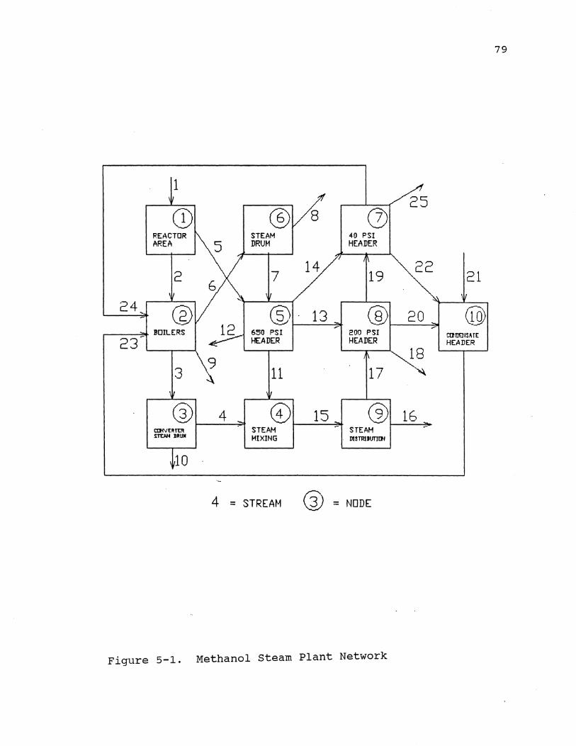
79

1 III ®Vs 25 CD (J)

REACTOR STEAM 40 PSI AREA 5 DRUM HEADER

2 7 14

19 22

21 6

" 24 ~ ® ® 13 ® 20 erg

)5- "'" ..-

- BOILERS 650 PSI 200 PSI CIlID01SAT[

23 HEADER HEADER HEADER

9 18

3 11 17 '~

I~ II

® 4 ~ cD 15 @ 16

STEAM - STEAM -CDNERTt:R Sn:AH lIRUM MIXING . DtSTRIIUT1[Jf

~10

4 = STREAM ® = NODE

Figure 5-1. Methanol steam Plant Network

80

Table 5-1. True and Observed Flow Rate Measurements for Methanol Plant.

True Observed stream Flow Rate Flow Rate

1 296.6 289.94 2 50.6 85.41 3 117.2 113.86 4 115.3 120.81 5 246 241. 81 6 244.8 248.39 7 243 245.53 8 1.8 1. 79 9 4.7 4.55

10 1.9 1.89 11 84.7 83.09 12 70.2 71.3 13 132 67.9 14 202.1 203.55 15 200 202.19 16 188 90.07 17 12 12.31 18 102.6 104.31 19 35.7 35.52 20 5.7 5.48 21 264.6 274.32 22 37.1 37.49 23 307.4 298.31 24 8.7 8.33 25 192 193.42

81

subject to the measurement errors of the measuring instru­

ment. Tables 5-2 and 5-3 demonstrate the objective function

using equation 5.2, subject to the nodal constraints using

equation 5.3.

The Lagrange multipliers are introduced in Table 5-4.

The multiplier is indicated by the letter r. To solve this

set of nonlinear equations, partial derivatives are taken

using equations 4 and 5 as demonstrated in Table 5-5. This

set of" 36 equations and 36 unknowns can be solved using

routine matrix procedures. The matrix is given in Table

5-6.

Lotus 123 simplifies the solution of this matrix

through the use of the data, matrix, inversion and data,

matrix, multiply commands. The left hand side of the matrix

is inverted and then multiplied by the right hand side. The

solution is given in Table 5-7. The new reconciled flow

rates are given along with the true and observed flow rates.

Lotus 123 is also used as a check to ensure that each nodal

constraint equation is balanced, i.e., that the sum of the

inflows minus the sum of the outflows equals zero.

Network Optimization using Linear Programming

Two additional strategies for optimally adjusting

erroneous hydraulic network flows have been introduced.

They are the methods of minimizing the sum of the absolute

values of the errors:

(5.6)

82

Table 5-2. Minimizing the Sum of the Normalized Errors Squared.

Objective function: Min (Xi-Xi*) "2/oi"2 for each i

Minimize Z=( X 1 - 289. )"2 / 7.415 "2 + ( X 2 - 85.4 )"2 / 1.265 "2 + ( X 3 - 113. )"2 / 2.930 "2 + ( X 4 - 120. )"2 / 2.883 "2 + ( X 5 - 241. )"2 / 6.150 "2 + ( X 6 - 248. )"2 / 6.120 "2 + ( X 7 - 245. )"2 / 6.075 "2 + ( X 8 - 1.79 )"2 / 0.045 "2 + ( X 9 - 4.55 )"2 / 0.118 "2 + ( X10 - 1.89 )"2 / 0.048 "2 + ( X11 - 83.0 )"2 / 2.118 "2 + ( X12 - 71. 3 )"2 / 1.755 "2 + ( X13 - 67.9 ) "2 / 3.300 "2 + ( X14 - 203. )"2 / 5.053 "2 + ( X15 - 202. )"2 / 5.000 "2 + ( X16 - 90.0 )"2 / 4.700 "2 + ( X17 - 12.3 )"2 / 0.300 "2 + ( X18 - 104. )"2 / 2.565 "2 + ( X19 - 35.5 )"2 / 0.893 "2 + ( X20 - 5.48 )"2 / 0.143 "2 + ( X21 - 274. )"2 / 6.615 "2 + ( X22 - 37.4 )"2 / 0.928 "2 + ( X23 - 298. )"2 / 7.685 "2 + ( X24 - 8.33 )"2 / 0.218 "2 + ( X25 - 193. )"2 / 4.800 "2

subject to: X1-X2-X5 = 0 X2+X23+X24-X3-X6-X9 = 0 X3-X4-X10 = 0 X4+X11-X15 = 0 X5+X7-X11-X12-X13-X14 = 0 X6-X7-X8 = 0 X14+X19-X22-X24-X25 = 0 X13+X17-X18-X19-X20 = 0 X15-X16-X17 = 0 X20+X21+X22-X23 = 0 X8+X9+X10+X12+X16+X18+X25-X1-X21 = 0

83

Table 5-3. Minimizing the Sum of the Normalized Errors Squared.

Minimize Z= 0.02 X 1 "2 --10.55 X 1 + 1528.95 + 0.62 X 2 "2 -106.75 X 2 + 4558.65 + 0.12 X 3 "2 -26.53 X 3 + 1510.10 + 0.12 X 4 "2 -29.08 X 4 + 1756.58 + 0.03 X 5 "2 -12.79 X 5 + 1545.96 + 0.03 X 6 "2 -13.26 X 6 + 1647.27 + 0.03 X 7 "2 -13.31 X 7 + 1633.49 +

493.83 X 8 "2 -1767.90 X 8 + 1582.27 + 72.43 X 9 "2 -659.12 X 9 + 1499.50 +

443.21 X10 "2 -1675.35 X10 + 1583.20 + 0.22 X11 "2 -37.06 X11 + 1539.75 + 0.32 X12 "2 -46.30 X12 + 1650.54 + 0.09 X13 "2 -12.47 X13 + 423.36 + 0.04 X14 "2 -15.95 X14 + 1623.04 + 0.04 X15 "2 -16.18 X15 + 1635.23 + 0.05 X16 "2 -8.15 X16 + 367.25 +

11.11 X17 "2 -273.56 X17 + 1683.73 + 0.15 X18 "2 -31. 71 X18 + 1653.78 + 1. 26 X19 "2 -89.18 X19 + 1583.91 +

49.25 X20 "2 -539.74 X20 + 1478.87 + 0.02 X21 "2 -12.54 X21 + 1719.71 + 1.16 X22 "2 -87.16 X22 + 1633.82 + 0.02 X23 "2 -10.10 X23 + 1506.77 +

21.14 X24 "2 -352.17 X24 + 1466.80 + 0.04 X25 "2 -16.79 X25 + 1623.75

subject to: X1-X2-X5 = 0 X2+X23+X24-X3-X6-X9 = 0 X3-X4-X10 = 0 X4+X11-X15 = 0 X5+X7-X11-X12-X13-X14 = 0 X6-X7-X8 = 0 X14+X19-X22-X24-X25 = 0 X13+X17-X18-X19-X20 = 0 X15-X16-X17 = 0 X20+X21+X22-X23 = 0 X8+X9+X10+X12+X16+X18+X25-X1-X21 = 0

84

Table 5-4. Introduction of Lagrange multipliers.

0.02 X 1 "2 -10.55 X 1 + 1528.95 + 0.62 X 2 "2 -106.75 X 2 + 4558.65 + 0.12 X 3 "2 -26.53 X 3 + 1510.10 + 0.12 X 4 "2 -29.08 X 4 + 1756.58 + 0.03 X 5 "2 -12.79 X 5 + 1545.96 + 0.03 X 6 "2 -13.26 X 6 + 1647.27 + 0.03 X 7 "2 -13.31 X 7 + 1633.49 +

493.83 X 8 "2 -1767.90 X 8 + 1582.27 + 72.43 X 9 "2 -659.12 X 9 + 1499.50 +

443.21 X10 "2 -1675.35 X10 + 1583.20 + 0.22 X11 "2 -37.06 X11 + 1539.75 + 0.32 X12 "2 -46.30 X12 + 1650.54 + 0.09 X13 "2 -12.47 X13 + 423.36 + 0.04 X14 "2 -15.95 X14 + 1623.04 + 0.04 X15 "2 -16.18 X15 + 1635.23 + 0.05 X16 "2 -8.15 X16 + 367.25 +

11.11 X17 "2 -273.56 X17 + 1683.73 + 0.15 X18 "2 -31. 71 X18 + 1653.78 + 1. 26 X19 "2 -89.18 X19 + 1583.91 +

49.25 X20 "2 -539.74 X20 + 1478.87 + 0.02 X21 "2 -12.54 X21 + 1719.71 + 1.16 X22 "2 -87.16 X22 + 1633.82 + 0.02 X23 "2 -10.10 X23 + 1506.77 +

21.14 X24 "2 -352.17 X24 + 1466.80 + 0.04 X25 "2 -16.79 X25 + 1623.75 +

r1*(X1-X2-X5) + r2*(X2+X23+X24-X3-X6-X9) + r3*(X3-X4-X10) + r4*(X4+X11-X15) + r5*(X5+X7-X11-X12-X13-X14) + r6*(X6-X7-X8) + r7*(X14+X19-X22-X24-X25) + r8*(X13+X17-X18-X19-X20) + r9*(X15-X16-X17) + r10*(X20+X21+X22-X23) + r11*(X8+X9+X10+X12+X16+X18+X25-X1-X21)

85

Table 5-5. Partial Derivatives.

dLjdX 1 = 0.04 X 1 -10.55 +r1-r11 dLjdX 2 = 1.25 X 2 -106.75 -r1+r2 dLjdX 3 = 0.23 X 3 -26.53 -r2+r3 dLjdX 4 = 0.24 X 4 -29.08 -r3+r4 dLjdX 5 = 0.05 X 5 -12.79 -r1+r5 dLjdX 6 = 0.05 X 6 -13.26 -r2+r6 dLjdX 7 = 0.05 X 7 -13.31 +r5-r6 dLjdX 8 = 987.65 X 8 -1767.90 -r6+r11 dLjdX 9 = 144.86 X 9 -659.12 -r2+r11 dLjdX10 = 886.43 X10 -1675.35 -r3+r11 dLjdX11 = 0.45 X11 -37.06 +r4-r5 dLjdX12 = 0.65 X12 -46.30 -r5+r11 dLjdX13 = 0.18 X13 -12.47 -r5+r8 dLjdX14 = 0.08 X14 -15.95 -r5+r7 dLjdX15 = 0.08 X15 -16.18 -r4+r9 dLjdX16 = 0.09 X16 -8.15 -r9+r11 dLjdX17 = 22.22 X17 -273.56 +r8-r9 dLjdX18 = 0.30 X18 -31. 71 -r8+r11 dLjdX19 = 2.51 X19 -89.18 +r7-r8 dLjdX20 = 98.49 X20 -539.74 -r8+r10 dLjdX21 = 0.05 X21 -12.54 +r10-r11 dLjdX22 = 2.32 X22 -87.16 -r7+r10 dLjdX23 = 0.03 X23 -10.10 +r2-r10 dLjdX24 = 42.28 X24 -352.17 +r2-r7 dLjdX25 = 0.09 X25 -16.79 -r7+r11 dLjdr 1 =X1-X2-X5 dLjdr 2 =X2+X23+X24-X3-X6-X9 dLjdr 3 =X3-X4-X10 dLjdr 4 =X4+X11-X15 dLjdr 5 =X5+X7-X11-X12-X13-X14 dLjdr 6 =X6-X7-X8 dLjdr 7 =X14+X19-X22-X24-X25 dLjdr 8 =X13+X17-X18-X19-X20 dLjdr 9 =X15-X16-X17 dLjdr10 =X20+X21+X22-X23 dLjdr11 =X8+X9+X10+X12+X16+X18+X25-X1-X21

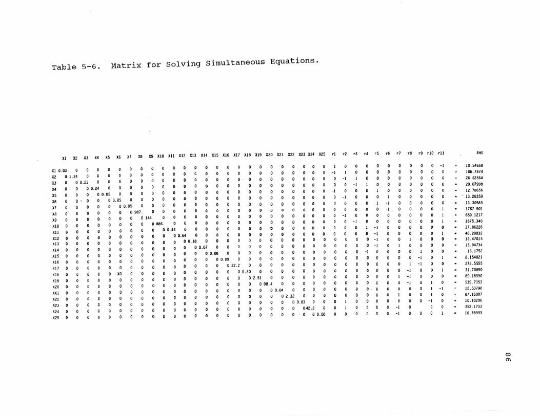
Table 5-6. Matrix for Solving Simultaneous Equations.

XI X2 X3 X4 XS X6 X7 X8 X9 XIO xu XI2 XI3 XI4 XIS XI6 XI7 XI8 XI9 X20 X21 X22 X23 X24 X2S rl r2 r3 r4 rS r6 r7 r8 r9 riO r11

XI 0.03 0 0 X2 0 1. 24 0 0 0 0 0

X3 0 0 0.23 0 0 0

X40 00.24 0

XS 0 O. 0 0.05 0 X6 0 0 0 0.05 0

o o o

o o

o 0

o

o o

o o 0 o 0

o 0

o 0

o 0

o 0 G 0 v o () o 0 o 0

o 0 X7 0 0 0 0.05 o 987. 0 0 0 0

X8

X9

XIO

XU XI2 XI3

o o o o o

o o

XI4

XIS

o o

o

o

o

o o o o o o o

o

o

o o o

o 01«. 0 0 0 0 o 0 886. 0 0 0 0

o 0 0 0 0.44 0 0 0

o 0 0 0 0 0.64 0 0 0 o 0 0 0 0.18 0

o 0 0 0 0 0.07

o o o 0.()8

o o

o o o o o o o o

XI6 o 0 0.09

o o o

o o

o

o 0

o 0 o o o o o

o o o

Xl7 o XO

o 0 0 0

00000 00

00000 00

o 0 0 22.2 0

o o o o 0 0 0 0.30

o o o o o o o o '0

o o

o

o o

o 0 0

o 0 0

o 0 o 0 0

o 0 0 0

o 0 0 0

o o o o o o o

o o

o o o o o o o

o o

o o

o o o o o o o o

o o o o o

o

o

o -I o -I

-I -I 0 0

o o

o -I 0

o o

o

-I

o o

-I

o 0 0

00.0

o 0 o

O· 0

I 0 1

o

o 0 o 0

o o

1 -1 o

o o 0

I -I -I

o -I o -I

-I 0 o 0

o

-1 0

o o o 0 o 0 o o o 0

o o 0

o

o 0

o o o 0

o 0

o 0

I -I

1 -I

-1 0 XI8

XI9 o 0 o 2.51 0 0 0 0 o -1

X20

XXI

X22

X23

X24 0 0

X25 0 0

o o 0

o 0 o

o 0

o o o o

o 0

o 0

o

o o

o

o 0 98.4 0 0 0 0 0

o 0.04 0 0 0

o 0 2.32 0

o 0 0 0.03 0

o o 0 0 042.2 0

o 0 0 O. ()8

o 0

o 0 0

o

o -I o 0 o -I 0

000 -I -1

o -I o

o 0

o 0 o

o o o o o o o o

o

o 1 o

o 0

I 0 -I

I 0

-I 0

RHS

10.54668

106.7474

26.52564

29.07998 12.78656

• .' 13.26359

13.30583

1767.901

659.1217

1675.346

37.06226

46.29832 12.47015

15.94734

16.1752

8.154821

273.5555

31. 70890

89.18390

539.7353

12.53798

87.16007

10.10206

352.1733

16.78993

00 (j\

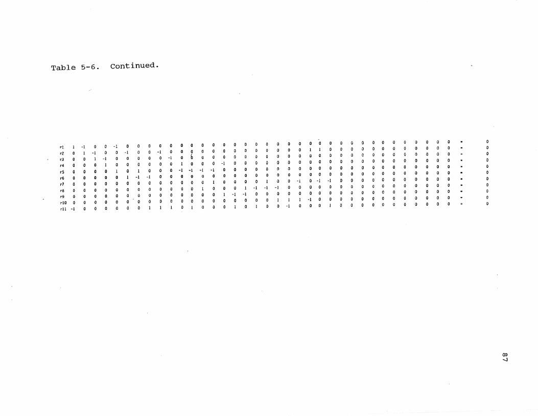
Table 5-6. continued.

rl

r2 r3

r4

r5 r6

r7 r8

o o o o o

-1

1 o o o o o

r9 0 0

rIO 0 0 rll -1 0

-1

1

o o o o

o o

-1

1 o o o

-1

o o

o o

o 0 0 o o. 0

o 0 0 o 0

o -1

o o o 1 o o o o o

o o o 1

-1 o o o o

o o a a

-1

o o o 1

a -1

o a a o o o

o o

-1

o o o o

o 0

o

o 0

~ 6 1 0

-1 -1 o 0

o 0 o 0 o 0

o a

o o o

-1 o o 1

o

o

o o

a -1 o 1

o

o -I o o o

a o o o o

o a o o o o

o o o o o o o

o o o a o o 1

o o o o o o o

o o o o o o o

o 0 0 -1 -I -1 0

o 1 -I -1 0 0 0 0 o 0 0 0 0 o 00 1 0 0 -1

o o o o o o

-1

o 0 0

1 1 a o 0

o 0

o 0 0

o 0 0 o -I -1

o o a o o o

o o o o o o o

a 0 0 o 0 0

o 0 0 -1 0

o 0 0

o 0 0

o 0 a 1 0 a

o o

o o

o o o o o o o

o a a o

a o

o 0 0 o 0 0

o 0 0

o 0 a

a o a o o a o o o o o

o o o o o o o o o o o

o o o o o o o o o o o

o o o o o o o o o

o o o o o o o o o o o

o o o o o o o o o o

o

o o o o o

o o

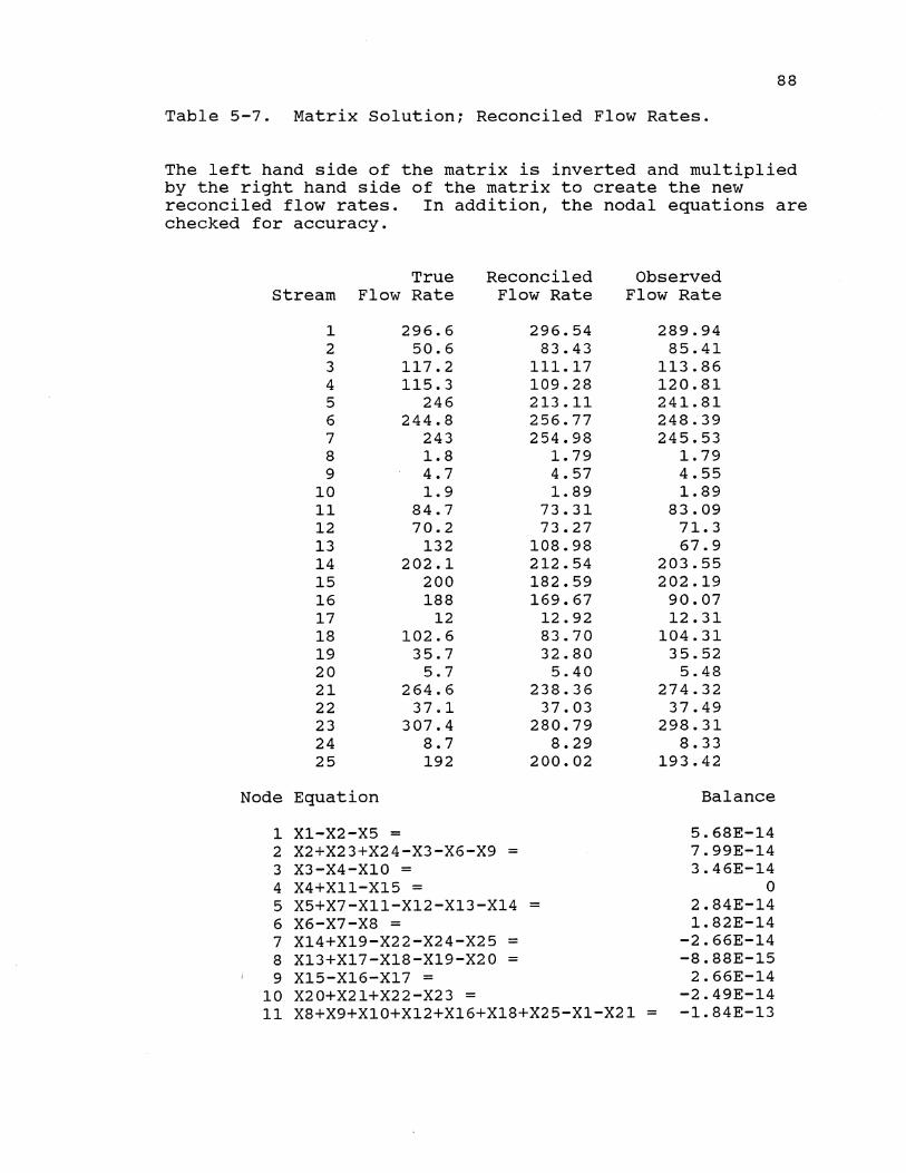
88

Table 5-7. Matrix Solution; Reconciled Flow Rates.

The left hand side of the matrix is inverted and multiplied by the right hand side of the matrix to create the new reconciled flow rates. In addition, the nodal equations are checked for accuracy.

True Reconciled Stream Flow Rate Flow Rate

1 296.6 2 50.6 3 117.2 4 115.3 5 246 6 244.8 7 243 8 1.8 9 4.7

10 1.9 11 84.7 12 70.2 13 132 14 202.1 15 200 16 188 17 12 18 102.6 19 35.7 20 5.7 21 264.6 22 37.1 23 307.4 24 8.7 25 192

Node Equation

1 X1-X2-X5 = 2 X2+X23+X24-X3-X6-X9 = 3 X3-X4-X10 = 4 X4+X11-X15 =

296.54 83.43

111.17 109.28 213.11 256.77 254.98

1. 79 4.57 1.89

73.31 73.27

108.98 212.54 182.59 169.67

12.92 83.70 32.80 5.40

238.36 37.03

280.79 8.29

200.02

5 X5+X7-XII-X12-X13-X14 = 6 X6-X7-X8 = 7 X14+X19-X22-X24-X25 = 8 X13+X17-X18-X19-X20 = 9 X15-X16-X17 =

10 X20+X21+X22-X23 =

Observed Flow Rate

289.94 85.41

113.86 120.81 241.81 248.39 245.53

1.79 4.55 1.89

83.09 71.3 67.9

203.55 202.19

90.07 12.31

104.31 35.52

5.48 274.32

37.49 298.31

8.33 193.42

Balance

5.68E-14 7.99E-14 3.46E-14

o 2.84E-14 1. 82E-14

-2.66E-14 -8.88E-15

2.66E-14 -2.49E-14

11 X8+X9+X10+X12+X16+X18+X25-X1-X21 = -1.84E-13

89

where

and minimizing the maximum error of any stream:

Min Max ei (5.7)

The above strategies are solved using linear program­

ming procedures (Bradley et al., 1977; Hillier and

Lieberman, 1967; Schrage, 1984). At this point a new

wastewater distribution network (Figure 5-2) is introduced

with a tableau, more familiar to linear programming proce­

dures (Table 5-8). Only those flows which connect two nodes

exist and are known as arcs. An arc is numbered according

to the direction of flow and the nodes which it connects.

For example, the arc X2625 indicates the arc is between

nodes 26 and 25, and the direction of flow is from node 26

to node 25. The flows into or out of the environment have

been removed and their values are now located within the

parentheses at their respective nodes. Notice that in the

tableau (Table 5-8) the 16 nodes are listed vertically on

the left, the arcs are listed horizontally across the top,

and the flows entering or leaving the network are listed

horizontally with their respective nodes on the right hand

side.

There are three types of nodes (Bradley et al., 1977;

Hillier and Lieberman, 1967). A source node supplies water

to the network. In the network the source nodes are nodes

27, 32, 35, 38, 41, and 43. Sink nodes are those nodes

KANAPAHA VASTE VATER TREATHENT PLANT

X25TP

X2625 X2926 r-----~~------~2

,-/X3029

~ ~/x;130 ~ .

X3231 l®

Figure 5-2. waste water collection Network

90

Table 5-8. Linear programming Formulation.

Actual Stream Values

1000 1000 300 700 50 50 50 650 150 500 200 300 100 200' 300

Stream X25TP X2625 X2726 X2926 X3029 X3130 X3231 X3429 X3534 X3734 X3837 X4045 X4140 X4340 X4537 RHS

Node 25 -1 Node 26 ' -1 -1 Node 27 1 Node 29 -1

Node 30 1 -1

Node 31 Node 32 Node 34 Node 35 Node 37 Node 38 Node 40 Node 41 Node 43 Node 45 Node TP -1

-1

-1 1

-1 -1 1

-1

1

-1 -1 1

1

-1

-1

o o

300 o o o

50 o

150 o

200 o

100 200

o -1000

~ f-'

92

where water is in demand. The demand node is the waste

water treatment plant node TP. The last type of node is a

trans-shipment node where there is no net supply or demand.

In this network, nodes 25, 26, 29, 30, 31, 34, 37, 45, and

40 are transshipment nodes.

The 10 equations that are depicted within the tableau

are the flow balance equations at each node. Each equation

satisfies the conservation of flow law:

(Flow out of node)-(Flow into node)=Net supply (5.8)

within the tableau, a 1 indicates flow out of a node and a

-1 indicates flow into a node. As an example, at node 25,

the balance equation is:

X25TP - X2625 = 0 (5.9)

A positive right hand side indicates that water is supplied

to the network at that node. A quick check will verify that

each stream is listed in two equations within the tableau,

once as an input and once as an output.

Comparison of the Three Network optimization strategies

All three optimization strategies: minimizing the sum

of the normalized errors squared, minimizing the sum of the

absolute value of the errors, and minimizing the maximum

error were tested on the waste water treatment network.

Each method was tested using five sets of data. The five

data sets contain no gross errors (Table 5-9). All errors

are random, which is defined as within a standard deviation

of 5% of the actual or true stream flow values. Random

Table 5-9. Random Error Test Cases.

Comparison of three optimization strategies on five test cases which include only random errors.

Observed Flow Rate

I Actual stream Flow Rate Test 1 Test 2 Test 3 Test 4 Test 5

X4340 200 196.25 198.04 201. 91 196.77 198.13 X4140 100 99.64 95.7 101.98 100.57 102.35 X4045 300 314.67 286.35 306.09 314.37 313.17 X4537 300 288.48 304.89 308.79 304.1 285.15 X3837 200 199.05 202.39 206.86 196.8 204.55 X3734 500 503.85 482.77 488.44 475.51 512.8 X3534 150 142.63 153.53 154.41 142.74 157.31 X3429 650 674.74 660.51 662.03 648.64 648.59 X3231 50 51.91 48.82 51.87 50.7 49.38 X3130 50 52.12 48.81 47.84 51.38 48.07 X3029 50 51.95 51.58 49.49 50.95 48.91 X2926 700 678.49 724.45 723.01 681. 94 684.82 X2726 300 310.06 292.01 286.37 296.17 307.37 X2625 1000 958.2 993.87 973.5 967.38 1046.88 X25TP 1000 980.59 965.12 1000.57 969.43 1024.85

~ w

94

errors are imposed on the actual flow data set using the

random number generator in Lotus 123.

Least Errors Squared Analysis

Table 5-10 gives the objective function and constraints

for minimizing the sum of the normalized errors squared on

the first data set. The method of solution is similar to

the methanol network discussed previously. Tables 5-11 and

5-12 display the objective function and constraints, using

the strategies of minimizing the sum of the absolute value

of the errors and minimizing the maximum error, respec­

tively, on the first data set.

Least Absolute Value Analysis

To solve the problem of minimizing the sum of the

absolute value of the errors using linear programming (Table

5-11), the errors, ei, are defined as Ui-Vi. This is

required since linear programming is designed for variables

constrained to be non negative. The objective function and

constraints are defined in the following form (Schrage,

1984):

subject to

Ui-Vi+Xi = Xi* for all i, and

~iaijXi = 0 for each node.

(5.10)

(5.11)

(5.12)

Equa~ion 5.11 represents the constraint that the error,

Ui-Vi, plus the corrected or reconciled flow, Xi, equals the

95

Table 5-10. Minimizing the Sum of the Normalized Errors Squared.

Minimize Z= ( X4340 - 196.25 )"2 / 10 "2 + ( X4140 99.64 )"2 / 5 "2 + ( X4045 - 314.67 )"2 / 15 "2 + ( X4537 - 288.48 )"2 / 15 "'2 + ( X3837 - 199.05 )"2 / 10 "'2 + ( X3734 - 503.85 )"2 / 25 "2 + ( X3534 - 142.63 )"2 / 7.5 "2 + ( X3429 - 674.74 )"2 / 32.5 "'2 + ( X3231 - 51.91 )"2 / 2.5 "'2 + ( X3130 - 52.12 )"2 / 2.5 "2 + ( X3029 - 51.95 )"2 / 2.5 "2 + ( X2926 - 678.49 )"2 / 35 "2 + ( X2726 - 310.06 )"2 / 15 "2 + ( X2625 - 958.2 )"2 / 50 "2 + ( X25TP - 980.59 )"2 / 50 "2

subject to: X4340+X4140-X4045 = 0

X4045-X4537 = 0 X4537+X3837-X3734 = 0 X3734+X3534-X3429 = 0 X3231-X3130 = 0 X3130-X3029 = 0 X3429+X3029-X2926 = 0 X2926+X2726-X2625 = 0 X2625-X25TP = 0 X4340+X4140+X3837+X3534+X3231+X2726-X25TP = 0

\

96

Table 5-11. Minimizing the Sum of the Absolute Values of of the Errors

MIN U1 + V1 + U2 + V2 + U3 + V3 + U4 + V4 + U5 + V5 + U6 + V6 + U7 + V7 + U8 + V8 + U9 + V9 + U10 + V10 + U11 + V11 + U12 + V12 + U13 + V13 + U14 + V14 + U15 + V15

SUBJECT TO 2) 3) 4) 5) 6) 7) 8) 9)

10) 11) 12) 13} 14) 15) 16} 17) 18) 19) 20) 21)

--More--6) 7) 8) 9)

10) 11} 12) 13) 14) 15) 16) 17) 18) 19) 20) 21)

--More--22) 23) 24) 25) 26)

END

U1 - V1 + X4340 = U2 - V2 + X4140 = U3 - V3 + X4045 = U4 - V4 + X4537 = U5 - V5 + X3837 = U6 - V6 + X3734 = U7 - V7 + X3534 = U8 - V8 + X3429 = U9 - V9 + X3231 = U10 - V10 + X3130 = U11 - V11 + X3029 = U12 - V12 + X2926 = U13 - V13 + X2726 = U14 - V14 + X2625 =

196.25 99.64

314.67 288.48 199.05 503.85 142.63 674.74

51.91 52.12 51.95

678.49 310.06 958.2 980.59 U15 - V15 + X25TP =

X4340 + X4140 - X4045 = X4045 - X4537 = 0 X4537 + X3837 - X3734 = X3734 + X3534 - X3429 = X3231 - X3130 = 0

o

o o

U5 - V5 + X3837 = U6 - V6 + X3734 = U7 - V7 + X3534 = U8 - V8 + X3429 = U9 - V9 + X3231 = U10 - V10 + X3130 = U11 - V11 + X3029 = U12 - V12 + X2926 = U13 - V13 + X2726 = U14 - V14 + X2625 =

199.05 503.85 142.63 674.74

51.91 52.12 51.95

678.49 310.06 958.2 980.59 U15 - V15 + X25TP =

X4340 + X4140 - X4045 = o X4045 - X4537 = 0 X4537 + X3837 - X3429 = X3734 + X3534 - X3429 = X3231 - X3130 = 0

X3130 - X3029 = 0

o o

X3429 + X3029 - X2926 = 0 X2926 + X2726 - X2625 = 0 X2625 - X26TP = 0 X4340 + X4140 + X3837 + X3534 + X3231 + X2726 - X25TP = 0

97

Table 5-12. Minimizing the Maximum Error

MIN Z

SUBJECT TO 2) Ul - VI + X4340 = 196.25 3) U2 - V2 + X4140 = 99.64 4) U3 - V3 + X4045 = 314.67 5) U4 - V4 + X4537 = 288.48 6) U5 - V5 + X3837 = 199.05 7) U6 - V6 + X3734 = 503.85 8) U7 - V7 + X3534 = 142.63 9) U8 - V8 + X3429 = 674.74

10) U9 - V9 + X3231 = 51. 91 11) U10 - V10 + X3130 = 52.12 12) U11 - VII + X3029 = 51.95 13) U12 - V12 + X2926 = 678.49 14) U13 - V13 + X2726 = 310.06 15) U14 - V14 + X2625 = 958.2 16) U15 - V15 + X25TP = 980.59 17) Z - U1 - VI >= 0 18) Z - U2 - V2 >= 0 19) Z - U3 - V3 >= 0 20) Z - U4 - V4 >= 0 21) Z - U5 - V5 >= 0 22) Z - U6 - V6 >= 0 23) Z - U7 - V7 >= 0

--More--21) Z - U5 - V5 >= 0 22) Z - U6 - V6 >= 0 23) Z - U7 - V7 >= 0

--More--24) Z - U8 - V8 >= 0 25) Z - U9 - V9 >= 0 26) Z - U10 - V10 >= 0 27) Z - U11 - VII >= 0 28) Z - U12 - V12 >= 0 29) Z - U13 - V13 >= 0 30) Z - U14 - V14 >= 0 31) Z - U15 - V15 >= 0 32) X4340 + X4140 - X4045 = 0 33) X4045 - X4537 = 0 34) X4537 + X3837 - X3734 = 0 35 ) X3734 + X3534 - X3429 = 0 36) X3231 - X3130 = 0 37) X3130 - X3029 = 0 38) X3429 + X3029 - X2926 = 0 39) X2926 + X2726 - X2625 = 0 40) X2625 - X25TP = 0 41) X4340 + X4140 + X3837 + X3534 + X3231 + 2726

- X25TP = 0 END

98

observed flow, Xi*. Equation 12 is the nodal constraint

equation where the sum of inflows minus outflows must equal

zero.

At this point, it is assumed that neither the flows on

the left or right hand side of each equation are known to be

correct. If the external supply into and demand out of the

network was known, an optimal balance of the streams on the

left hand side of each node equation could be solved for.

Minimizing the Maximum Error

In using a linear program (Schrage, 1984), minimizing

the maximum error is expressed as follows (Table 5-12):

subject to

Min Z

Ui+Vi+Xi = Xi* for all i,

Z-Ui-Vi >= 0, for all i, and

iai~Xi = ° for each node.

In equation 5.13, Z represents the maximum error.

(5.13)

(5.14)

(5.15)

(5.16)

Equation 5.15 represents the constraint that Z >= Ui + Vi.

If the constraint sets 5.14, 5.15, and 5.16 are met, then

the least maximum error solution will be found when Z is

minimized.

The above three methods used for the optimization of

erroneous flows within the waste water network were con­

tinued on the next four data sets. In comparing the

results, the summation of the deviation between each true

flow rate and the corrected or reconciled flow rate is

99

calculated (Table 5-13). Minimizing the sum of the normal­

ized errors squared proved to be the best method in all but

one test case.

with this limited amount of test cases the least error

squared analysis would seem to be the best method to use in

the optimization of erroneous data, if the data contain only

random errors. But what if the data sets contain gross

errors?

optimization of Networks Involving Gross Errors

The three network optimization techniques are now used

in three test cases of the network where approximately 20%

of the streams received gross errors, i.e. the observed

value is greater than the standard deviation of 5% (Table

5-14). The rest of the streams contain random errors.

Lotus 123 was used with the random number function to create

the data sets.

When gross errors are imposed, minimizing the sum of

the absolute value of the errors is the best technique to

use in the optimization of data which contain gross errors.

Table 5-15 indicates the results. This method proved to be

best in each test when a comparison of the sum of the

deviations between true and reconciled data was made.

Gross Error Detection Algorythms

Five algorithms are currently being used in the

detection of gross errors, removing them, and optimally

adjusting the rest of the flows which are assumed to include

•

Table 5-13. Random Error Test Results.

TEST 1 Sum of deviation between

Reconciled flow rates: true and reconciled flow rates: LS LAV MINMAX LS LAV MINMAX

198.88 196.25 195.35 1.12 3.75 4.65 100.30 99.64 99.64 0.30 0.36 0.36 299.18 295.89 294.99 0.82 4.11 5.01 299.18 295.89 294.99 0.82 4.11 5.01 199.56 199.05 199.05 0.44 0.95 0.95 498.74 494.94 494.04 1. 26 5.06 5.96 142.46 131. 64 161.02 7.54 18.36 11.02 641. 20 626.58 655.06 8.80 23.42 5.06

51.92 51.91 32.44 1.92 1.91 17.56 51. 92 51.91 32.44 1. 92 1.91 17.56 51.92 51.91 32.44 1.92 1.91 17.56

693.12 678.49 687.50 6.88 21. 51 12.50 304.91 302.10 290.38 4.91 2.10 9.62 998.03 980.59 977.88 1. 97 19.41 22.12 998.03 980.59 977.88 1. 97 19.41 22.12

sum = 42.59 128.28 157.06

f-> o o

Table 5-13. continued.

TEST 2

Reconciled flow rates: LS LAV MINMAX

198.68 198.04 198.04 95.86 95.70 89.74

294.54 293.74 287.78 294.54 293.74 287.78 202.06 202.39 202.39 496.60 496.13 490.17 154.59 156.91 168.36 651.19 653.04 658.53

49.76 48.82 48.81 49.76 48.82 48.81 49.76 48.82 48.81

700.95 701. 86 707.34 289.96 292.01 274.90 990.91 993.87 982.23 990.91 993.87 982.23

Sum of deviation between true and reconciled flow rates:

LS LAV MINMAX

1. 32 1.96 1. 96 4.14 4.30 10.26 5.46 6.26 12.22 5.46 6.26 12.22 2.06 2.39 2.39 3.40 3.87 9.83 4.59 6.91 18.36 1.19 3.04 8.53 0.24 1.18 1.19 0.24 1.18 1.19 0.24 1.18 1.19 0.95 1.86 7.34

10.04 7.99 25.10 9.09 6.13 17.77 9.09 6.13 17.77

sum 57.55 60.64 147.32

I-' o I-'

Table 5-13. continued.

TEST 3

Reconciled flow rates: LS LAV MINMAX

20/1. 98 201.91 188.37 102.00 101. 98 106.88 303.98 303.89 295.25 303.98 303.89 295.25 203.86 203.73 206.72 507.84 507.62 501.97 154.47 154.41 167.94 662.30 662.03 669.92

49.74 51.87 39.55 49.74 51.87 39.55 49.74 51.87 39.55

712.04 713.90 709.47 284.64 286.37 277.56 996.67 1000.27 987.03 996.67 1000.27 987.03

sum =

Sum of deviation between true and reconciled flow rates:

LS LAV MINMAX

1.98 1.91 11. 63 2.00 1.98 6.88 3.98 3.89 4.75 3.98 3.89 4.75 3.86 3.73 6.72 7.84 7.62 1.97 4.47 4.41 17.94

12.30 12.03 19.92 0.26 1.87 10.45 0.26 1.87 10.45 0.26 1.87 10.45

12.04 13.90 9.47 15.36 13.63 22.44

3.33 0.27 12.97 3.33 0.27 12.197

75.25 73.14 163.76

...... o r.J

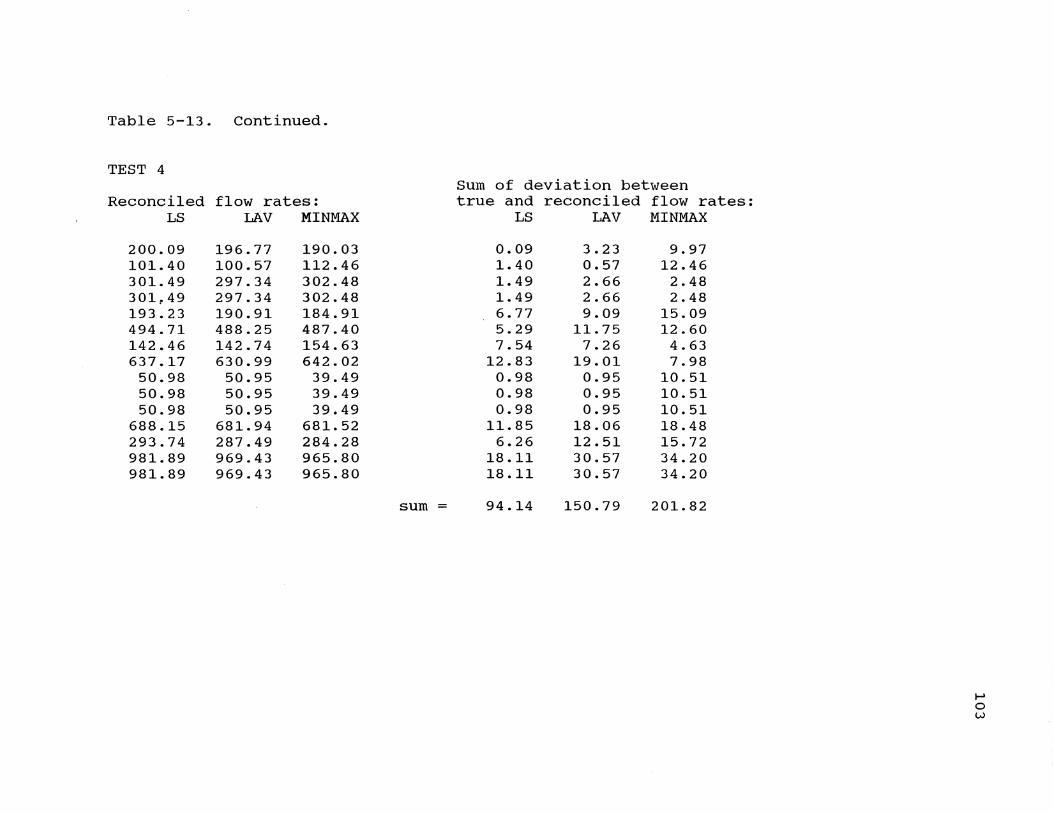
Table 5-13. continued.

TEST 4

Reconciled flow rates: LS LAV MINMAX

200.09 196.77 190.03 101.40 100.57 112.46 301. 49 297.34 302.48 301~49 297.34 302.48 193.23 190.91 184.91 494.71 488.25 487.40 142.46 142.74 154.63 637.17 630.99 642.02

50.98 50.95 39.49 50.98 50.95 39.49 50.98 50.95 39.49

688.15 681. 94 681. 52 293.74 287.49 284.28 981. 89 969.43 965.80 981. 89 969.43 965.80

Sum of deviation between true and reconciled flow rates:

LS LAV MINMAX

0.09 3.23 9.97 1. 40 0.57 12.46 1. 49 2.66 2.48 1.49 2.66 2.48 6.77 9.09 15.09 5.29 11. 75 12.60 7.54 7.26 4.63

12.83 19.01 7.98 0.98 0.95 10.51 0.98 0.95 10.51 0.98 0.95 10.51

11. 85 18.06 18.48 6.26 12.51 15.72

18.11 30.57 34.20 18.11 30.57 34.20

sum = 94.14 150.79 201.82

I-' o w

Table 5-13. continued.

TEST 5 Sum of deviation between

Reconciled flow rates: true and reconciled flow rates: LS LAV MINMAX LS LAV MINMAX

197.43 198.13 216.36 2.57 1.87 16.36 102.17 102.35 84.12 2.17 2.35 15.88 299.60 300.48 300.48 0.40 0.48 0.48 299.60 300.48 300.48 0.40 0.48 0.48 204.24 204.55 196.35 4.24 4.55 3.65 503.84 505.03 496.83 3.84 5.03 3.17 156.33 143.56 157.31 6.33 6.44 7.31 660.17 648.59 654.14 10.17 1.41 4.14

48.77 48.91 48.91 1. 23 1.09 1. 09 48.77 48.91 48.91 1.23 1. 09 1. 09 48.77 48.91 48.91 1. 23 1. 09 1. 09

708.95 697.50 703.05 8.95 2.50 3.05 310.35 327.35 325.60 10.35 27.35 25.60

1019.30 1024.85 1028.65 19.30 24.85 28.65 ,1019.30 1024.85 1028.65 19.30 24.85 28.65

sum = 91. 71 105.43 140.69

Results: Test LS LAV MINMAX

1 42.59 128.28 157.06 2 57.55 60.64 147.32 3 75.25 73.14 163.76 4 94.14 150.79 201. 82 5 91. 71 105.43 140.69

sum = 361. 24 518.28 810.65 ~ 0 01:=-

Table 5-14. Gross Error Test Cases.

Comparison of three optimization strategies on three test cases which include approximately 20% gross errors.

Actual stream Flow Rate Test 1

X4340 200 192.69 X4140 100 102.52 X4045 300 297.59 X4537 300 311.89 X3837 200 193.12 X3734 500 891 X3534 150 147.26 X3429 650 645.74 X3231 50 48.1 X3130 50 34.8 X3029 50 51. 58 X2926 700 692.94 X2726 300 93.65 X2625 1000 999.13 X25TP 1000 1044.18.

Observed Flow Rate

Test 2

196.2 98.5

289.52 58.53

205.76 295.98 142.88 669.28

70.65 48.63 49.63

707.68 496.98

1006.15 1684.8

Test 3

191. 25 137.01 448.85 314.13 206.4

516.85 148.16 674.24

51. 09 51.95 47.68

729.37 290.67 974.18

975.1

105

Table 5-15. Gross Error Test Results.

TEST 1 Sum of the deviation between

Reconciled flow rates: true and reconciled flow rates: LS LAV MINMAX LS LAV MINMAX

220.15 192.69 195.07 20.15 7.31 4.93 109.39 112.67 235.95 9.39 12.67 135.95 329.54 305.36 431.02 29.54 5.36 131. 02 329.54 305.36 431.02 29.54 5.36 131. 02 242.63 193.12 326.55 42.63 6.88 126.55 572.17 498.48 757.57 72.17 1. 52 257.57 146.41 147.26 21. 60 3.59 2.74 128.40 718.58 645.74 779.17 68.58 4.26 129.17

44.94 48.10 37.93 5.06 1.90 12.07 44.94 48.10 37.93 5.06 1.90 12.07 44.94 48.10 37.93 5.06 1.90 12.07

763.52 693.84 817.10 63.52 6.16 117.10 118.74 305.29 93.65 181. 26 5.29 206.35 882.26 999.13 910.75 117.74 0.87 89.25 882.26 999.13 910.75 117.74 0.87 89.25

sum = 771. 02 64.99 1582.77

~ o 0'1

Table 5-15. continued.

TEST 2

Reconciled flow rates: LS LAV MINMAX

146.17 191.02 0.00 85.99 98.50 58.53

232.17 289.52 58.53 232.17 289.52 58.53 207.41 205.76 435.62 439.58 495.28 494.15 156.73 162.77 482.20 596.31 685.05 976.35

56.67 49.63 70.65 56.67 49.63 70.65 56.67 49.63 70.65

652.98 707.68 1047.00 526.80 496.98 298.47

1179.79 1204.66 1345.47 1179.79 1204.66 1345.47

Sum of the deviation between true and reconciled flow rates:

LS LAV MINMAX

53.83 8.98 200.00 14.01 1. 50 41.47 67.83 10.48 241.47 67.83 10.48 241.47 7.41 5.76 235.62

60.42 4.72 5.85 6.73 12.77 332.20

53.69 35.05 326.35 6.67 0.37 20.65 6.67 0.37 20.65 6.67 0.37 20.65

47.02 7.68 347.00 226.80 196.98 1. 53 179.79 204.66 345.47 179.79 204.66 345.47

sum = 985.17 704.83 2725.85

I-' o -..J

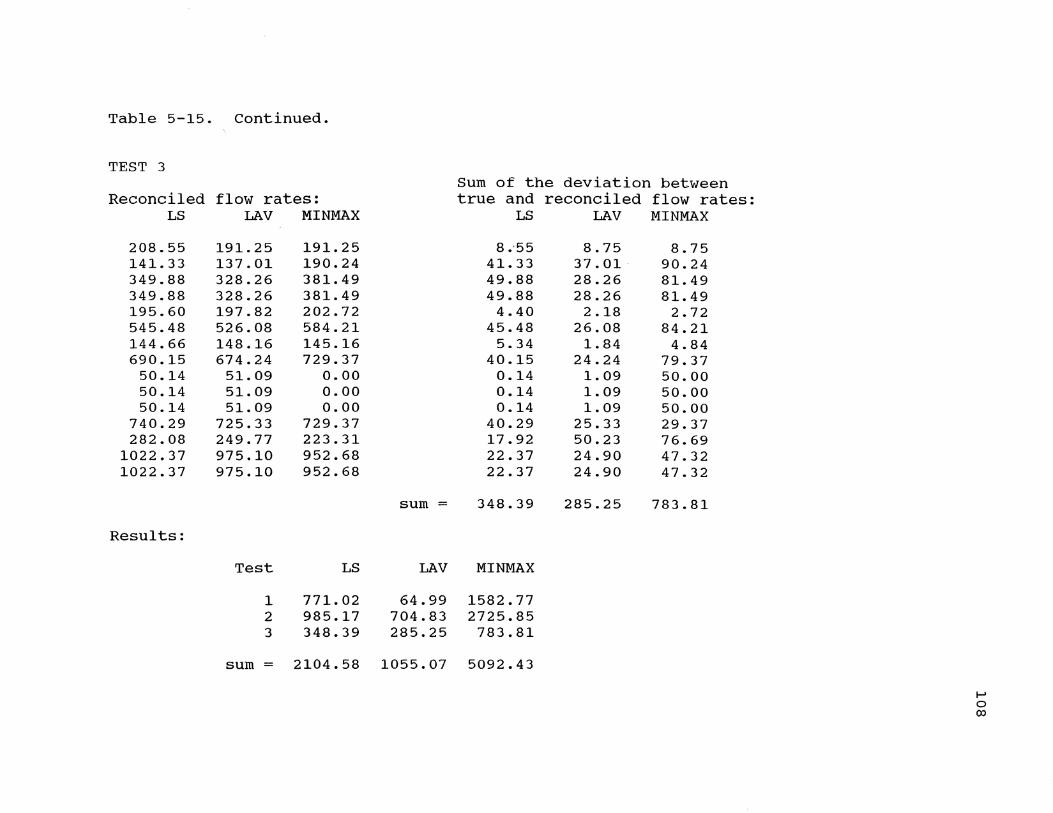
Table 5-15. continued.

TEST 3 Sum of the deviation between

Reconciled flow rates: true and reconciled flow rates: LS LAV MINMAX LS LAV MINMAX

208.55 191. 25 191. 25 8.'55 8.75 8.75 141. 33 137.01 190.24 41.33 37.01 90.24 349.88 328.26 381. 49 49.88 28.26 81.49 349.88 328.26 381.49 49.88 28.26 81. 49 195.60 197.82 202.72 4.40 2.18 2.72 545.48 526.08 584.21 45.48 26.08 84.21 144.66 148.16 145.16 5.34 1.84 4.84 690.15 674.24 729.37 40.15 24.24 79.37

50.14 51.09 0.00 0.14 1.09 50.00 50.14 51. 09 0.00 0.14 1.09 50.00 50.14 51.09 0.00 0.14 1.09 50.00

740.29 725.33 729.37 40.29 25.33 29.37 282.08 249.77 223.31 17.92 50.23 76.69

1022.37 975.10 952.68 22.37 24.90 47.32 1022.37 975.10 952.68 22.37 24.90 47.32

sum = 348.39 285.25 783.81

Results:

Test LS LAV MINMAX

1 771. 02 64.99 1582.77 2 985.17 704.83 2725.85 3 348.39 285.25 783.81

sum = 2104.58 1055.07 5092.43

~ 0 00

109

random errors. The algorithms have so far been described

for use in industrial processes, especially chemical, but

can also prove to be of value in the optimization of potable

and waste water hydraulic flow networks.

Measurement Test

The measurement test is the most straightforward of the

algorithms (Mah and Taffihane, 1982; Iordaache et al., 1985).

A statistical test is used to determine if there are any

gross errors. The test for gross errors is based on the

assumption that random errors are normally distributed.

After the data have been adjusted using the least error

squared analysis, a set of residuals is calculated:

(5.17)

The residuals are then tested to determine if any are

gross errors, known as outliers. For a 95% confidence level

an outlier is defined as

(5.18)

The general method is to detect which of the measure­

ments include gross errors. These measurements are removed

and replaced with more realistic values. Now, the network

is assumed to contain only random errors and the flows

within the network can be optimally adjusted and balanced so

that each node satisfies the condition of equation 5.1.

In the measurement test, all outliers are removed by a

process called nodal aggregation. The stream which has been

110

determined to be a gross error is removed from the data set

temporarily by combining the inflows and the outflows of the

two nodes, which the stream flows between, into one. The

least squared error analysis is reapplied to the new set of

data where outliers have been removed. The removed streams

are easily determined from the new set of Xi values.

Modified Iterative Measurement Test

The second algorithm is the modified iterative measure­

ment test (Serth and Heenan, 1986). This test is similar to

the measurement test. Once the initial least squared error

analysis is applied, the residuals calculated, and the

outliers identified, only the worst outlier is removed via

nodal aggregation and the least squared error analysis

applied. The new data set is then perused for unrealistic

flow rates, such as negative flow rates, or grossly large

positive ones. If unrealistic flow rates are present, the

outlier is put back in and the cycle is applied to the next

largest outlier until there are no more outliers among the

remaining residuals.

Pseudonodes Test

The pseudonodes test is the third algorithm (Mah et

al., 1976). Here, nodes are statistically tested for

imbalances. A nodal imbalance which has been statistically

normalized is defined as

(5. 19)

where

III

0:i = ( L: iO i.2) - 5 (5.20)

An outlier is a nodal imbalance which contains at least

one gross error and is defined by:

-1.96>O:i>1.96 (5.21)

Each node is tested successively. If the nodal

imbalance is not an outlier, its respective streams are

assumed to contain no gross errors and the streams are

removed from further consideration. Next, this procedure is

contained for aggregates of two nodes, called pseudonodes,

then aggregates of three nodes and so forth until no greater

number of aggregates can be formed. The streams that have

not been eliminated at the end of this procedure are assumed

to contain gross errors. These streams can then be replaced

through the method of nodal aggregation and least squared

error analysis as discussed in the measurement test.

Combinatorial Test

The combinatorial test is the forth algorithm (Serth

and Heenan, 1986). This method is similar to the pseudonode

test in that each individual node is tested for nodal

imbalances. The search is conducted for combinations of

gross errors which can explain the observed pattern of

imbalances. In other words, each single stream is assumed

to contain a gross error to see if that stream by itself

will cause the nodal imbalance. If no individual stream can

explain the nodal imbalances, then combinations of two

112

streams are tested, then combinations of three streams, and

so forth until no larger combination is possible. A very

large number of combinations is possible for even a small

number of streams.

Screened Combinatorial Test

The last algorithm is the screened combinatorial test

(Serth and Heenan, 1986). This method involves both the

pseudonode and combinatorial tests. The pseudonode test is

used to screen the initial data to identify the streams

which contain gross errors. The combinatorial test is then

applied to the reduced data which includes only those

streams identified to have gross errors.

Comparison of the Five Algorithms

The five algorithms were used to test 100 sets of data

(Heenan and Serth, 1986). A random number generator was

used to introduce both random and gross errors to a com­

pletely balanced original set of streams within a network.

Twenty percent of the flows were given gross errors. The

modified iterative measurement and the screened combina­

torial tests were the most accurate in identifying approxi­

mately 80% of the gross errors, with the least ~umber of

erroneous identifications, while reducing the total error

within the network by greater than 60%. Due to the better

efficiency, the modified iterative measurement test was the

method of choice (Heenan and Serth, 1986).

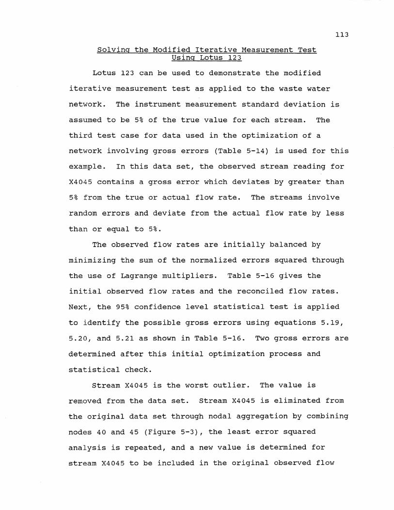
Solving the Modified Iterative Measurement Test Using Lotus 123

Lotus 123 can be used to demonstrate the modified

iterative measurement test as applied to the waste water

113

network. The instrument measurement standard deviation is

assumed to be 5% of the true value for each stream. The

third test case for data used in the optimization of a

network involving gross errors (Table 5-14) is used for this

example. In this data set, the observed stream reading for

X4045 contains a gross error which deviates by greater than

5% from the true or actual flow rate. The streams involve

random errors and deviate from the actual flow rate by less

than or equal to 5%.

The observed flow rates are initially balanced by

minimizing the sum of the normalized errors squared through

the use of Lagrange multipliers. Table 5-16 gives the

initial observed flow rates and the reconciled flow rates.

Next, the 95% confidence level statistical test is applied

to identify the possible gross errors using equations 5.19,

5.20, and 5.21 as shown in Table 5-16. Two gross errors are

determined after this initial optimization process and

statistical check.

Stream X4045 is the worst outlier. The value is

removed from the data set. Stream X4045 is eliminated from

the original data set through nodal aggregation by combining

nodes 40 and 45 (Figure 5-3), the least error squared

analysis is repeated, and a new value is determined for

stream X4045 to be included in the original observed flow

Table 5-16. Modified Iterative Measurement Test.

statistical test Recon- --------------------------------------------

True ciled (sigma)ei Flow Flow Observed ei= =true* ei/ Gross Worst

stream Rate Rate Flow Rate xi-xi* 5% (sigma)ei Error Outlier

X4340 200 208.55 191. 25 17.30 10 1. 73 NO X4140 100 141. 33 137.01 4.32 5 0.86 NO X4045 300 349.88 448.85 -98.97 15 -6.60 YES * X4537 300 349.88 314.13 35.75 15 2.38 YES X3837 200 195.60 206.40 -10.80 10 -1.08 NO X3734 500 545.48 516.85 28.63 25 1.15 NO X3536 150 144.66 148.16 -3.50 7.5 -0.47 NO X3429 650 690.15 674.24 15.91 32.5 0.49 NO X3231 50 50.14 51. 09 -0.95 2.5 -0.38 NO X3130 50 50.14 51. 95 -1.81 2.5 -0.72 NO X3029 50 50.14 47.68 2.46 2.5 0.98 NO X2926 700 740.29 729.37 10.92 35 0.31 NO X2726 300 282.08 290.67 -8.59 15 -0.57 NO X2625 1000 1022.37 974.18 48.19 50 0.96 NO X25TP 1000 1022.37 975.10 47.27 50 0.95 NO

t-' t-' .t:>

115

",.----

X4340 43

X4340

X4045 X4537

X4537

Figure 5-3. Nodal Aggregate to Eliminate stream X4045

116

rates as shown in Table 5-17. The new value for stream

X4045 is equal to stream X4537 or the sum of X4340 and X4140

which equals 320.88. The statistical test is conducted and

no gross errors are identified. If additional gross errors

were identified, the same procedure would be iterated until

no gross errors are identified after the statistical test.

A final least errors squared analysis is now repeated

using the original data set except for the value 320.88

which replaces the original observed flow rate for stream

X4045. The final reconciled flow rates are given in Table

5-18.

Comparison of Network Optimization with and Without Error Detection

A comparison between the reconciled values with and

without error detection can now be made for this single test

case. The use of the modified iterative measurement test

reduced the total sum of the deviation between the actual

flow rates and the reconciled flow rates by approximately

100% over the use of least errors squared optimization

without error detection (Table 5-19). The total deviation

is reduced from 348.39 to 174.30 through the use of the

modified iterative measurement test.

Conclusions

The conventional use of least errors squared analysis

and five algorithms, of which the modified iterative

measurement test was discussed in detail, in the industrial

process area have been demonstrated for use in the

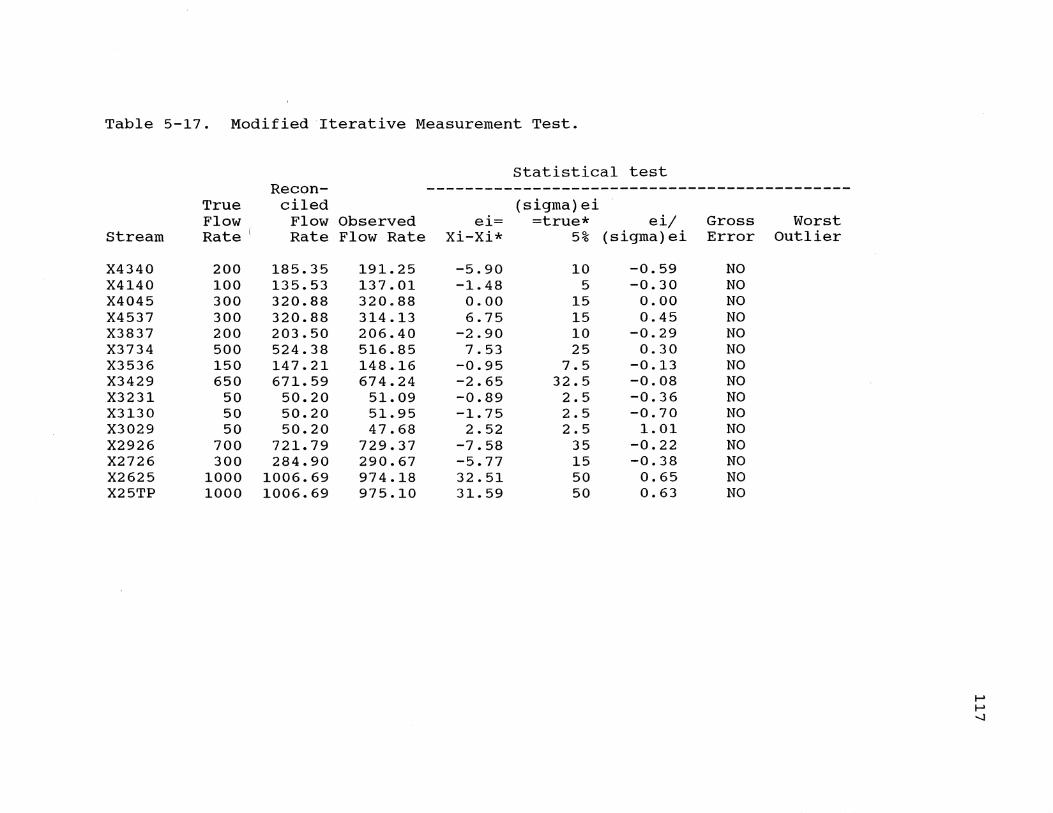
Table 5-17. Modified Iterative Measurement Test.

statistical test Recon- --------------------------------------------

True ciled (sigma)ei Flow. Flow Observed ei= =true* ei/ Gross Worst

stream Rate I Rate Flow Rate xi-Xi* 5% (sigma)ei Error Outlier

X4340 200 185.35 191.25 -5.90 10 -0.59 NO X4140 100 135.53 137.01 -1.48 5 -0.30 NO X4045 300 320.88 320.88 0.00 15 0.00 NO X4537 300 320.88 314.13 6.75 15 0.45 NO X3837 200 203.50 206.40 -2.90 10 -0.29 NO X3734 500 524.38 516.85 7.53 25 0.30 NO X3536 150 147.21 148.16 -0.95 7.5 -0.13 NO X3429 650 671. 59 674.24 -2.65 32.5 -0.08 NO X3231 50 50.20 51. 09 -0.89 2.5 -0.36 NO X3130 50 50.20 51.95 -1. 75 2.5 -0.70 NO X3029 50 50.20 47.68 2.52 2.5 1. 01 NO X2926 700 721. 79 729.37 -7.58 35 -0.22 NO X2726 300 284.90 290.67 -5.77 15 -0.38 NO X2625 1000 1006.69 974.18 32.51 50 0.65 NO X25TP 1000 1006.69 975.10 31.59 50 0.63 NO

~ ~ -...J

Table 5-18. Modified Iterative Measurement Test.

statistical test Recon- --------------------------------------------

True ciled (sigma)ei Flow Flow Observed ei= =true* eij Gross Worst

stream Rate Rate Flow Rate xi-xi* 5% (sigma)ei Error Outlier

X4340 200 181. 56 191. 25 -9.69 10 -0.97 NO X4140 100 134.59 137.01 -2.42 5 -0.48 NO X4045 300 316.15 316.15 0.00 15 0.00 NO X4537 300 316.15 314.13 2.02 15 0.13 NO X3837 200 204.79 206.40 -1. 61 10 -0.16 NO X3734 5001 520.94 516.85 4.09 25 0.16 NO X3536 150 147.62 148.16 -0.54 7.5 -0.07 NO X3429 650 668.56 674.24 -5.68 32.5 -0.17 NO X3231 50 50.21 51. 09 -0.88 2.5 -0.35 NO X3130 50 50.21 51.95 -1. 74 2.5 -0.70 NO X3029 50 50.21 47.68 2.53 2.5 1. 01 NO X2926 700 718.77 729.37 -10.60 35 -0.30 NO X2726 300 285.36 290.67 -5.31 15 -0.35 NO X2625 1000 1004.13 974.18 29.95 50 0.60 NO X25TP 1000 1004.13 975.10 29.03 50 0.58 NO

I-' I-' (Xl

Table 5-19. Comparison with and Without Error Detection.

Deviation Between True Reconciled Values and Reconciled Flow Rates ------------------- -------------------

with without True With without Observed Error Error Flow Error Error

stream Flow Rate Detection Detection Rate Detection Detection

X4340 191. 25 181.56 208.55 200 18.44 8.55 X4140 137.01 134.59 141. 33 100 34.59 41. 33 X4045 316.15 316.15 349.88 300 16.15 49.88 X4537 314.13 316.15 349.88 300 16.15 49.88 X3837 206.40 204.79 195.60 200 4.79 4.40 X3734 516.85 520.94 545.48 500 20.94 45.48 X3536 148.16 147.62 144.66 150 2.38 5.34 X3429 674.24 668.56 690.15 650 18.56 40.15 X3231 51. 09 50.21 50.14 50 0.21 0.14 X3130 51.95 50.21 50.14 50 0.21 0.14 X3029 47.68 50.21 50.14 50 0.21 0.14 X2926 729.37 718.77 740.29 700 18.77 40.29 X2726 290.67 285.36 282.08 300 14.64 17.92 X2625 974.18 1004.13 1022.37 1000 4.13 22.37 X25TP 975.10 1004.13 1022.37 1000 4.13 22.37

Sum = 174.30 348.39

~ ~ \.0

120

optimization of erroneous flows within a water distribution

network. Two additional methods for the optimization of a

network involving linear programming procedures were

introduced, minimizing the sum of absolute value of the

errors and minimizing the maximum error.

If all the errors are random, the method of minimizing

the sum of the errors squared was demonstrated to be the

most effective in minimizing the sum of the deviations

between actual and reconciled flow rates. When gross errors

are introduced, the method of minimizing the sum of the

absolute values of the errors was demonstrated to be the

method of choice. Also, use of gross error detection in the

modified iterative measurement test proves to reduce the

total error as demonstrated here and in prior research.

An interesting area for further research, for use when

gross errors are present, is the application of minimizing

the sum of the absolute value of the errors within the

modified iterative measurement test. since this method was

demonstrated to be the best of the network optimization

methods when gross errors are present in the data set, the

use of this method in the modified iterative measurement

test may provide an even better result in reducing the

deviation between true and reconciled flow values.

The statistical test used within the modified iterative

measurement test assumes that the errors are normally

distributed. Although this may not be the case, the method

121

has demonstrated to reduce the overall error when a network

is optimally balanced (Serth and Heenan, 1986).

CHAPTER VI SUMMARY AND CONCLUSIONS

Objectives

Use of microcomputers and ever more sophisticated

software packages are allowing a person to solve water

supply problems today that could only be solved with larger

computers previously. In this thesis, three different water

supply problems are solved. The first problem deals with

improving the knowledge base structure of a model which

determines preliminary design and cost for treating drinking

water with various water treatment processes.

The second problem involves improving the efficiency in

handling both input and output data of a model which

analyzes flow in pipe networks. The last water supply

problem concerns the optimization of water distribution

networks that include erroneous flows.

Electronic Spreadsheets

Throughout this thesis, Lotus 123 release 2 is used as

the mainstay to solve water supply problems. Lotus 123

effectively replaces calculation by hand and automates the

problem solving process. Included in Lotus 123 are a myriad

of commands and functions which make the spreadsheet a very

powerful and versatile tool for solving engineering

problems.

122

123

In this thesis, the macro programming language and the

matrix functions are used extensively. Matrix inversion and

multiplication commands are extremely helpful in the

solution of large sets of simultaneous equations. The

matrix commands are used in chapter V in the optimization of

erroneous network flows.

Decision Support System

The decision support system provides a framework for

solving a problem. In chapter III, the problem is to

determine the preliminary design and cost for various

potable water treatment processes. A Lotus 123 spreadsheet

supplies the system of rules, logical steps, and knowledge

bases to solve the problem. within the spreadsheet, the

required information for solving the problem is grouped

together within logical sections, i.e., chemical costs, cost

factors, influent water properties, and desired treatment

process sections. A macro menu system allows easy movement

around the spreadsheet and help messages for any problem

areas.

Lotus 123 excels in creating the knowledge base. Data

tables, graphs, figures, maps, and equations can be included

within the spreadsheet to document how the problem is

solved. The use of logarithmic graphs is of special

significance in providing water treatment cost estimates.

The knowledge base within the spreadsheet is easily updated

as the state of the art solution to the problem changes.

124

Data Handling

In chapter IV, a Lotus 123 spreadsheet is created to

pre- and postprocess data for use in a model which analyses

flow in a pipe network. Most of the time involved with

using this model or any other model is spent creating and

manipulating the data base. The spreadsheet can effectively

streamline data handling. Various functions provided by

Lotus 123, plus a macro incorporating the functions, creates

a very fast program which reduces data handling time. The

preprocessor can cut the data handling time by fifty percent

when used as opposed to the data input system provided by

the hydraulic network analysis model.

Another advantage in using the spreadsheet pre- and

postprocessors is with the help support system. As many

help messages as required can be included within the

spreadsheet. This allows one to stay within the processing

program and find needed assistance instead of searching

through a user's manual.

Spreadsheet Modeling

The Lotus 123 macro language is used in chapters III

and IV to create program to solve two different problems.

The macro designed for the water treatment model is simple

to use and involves much less programming language than the

water treatment model written in the BASIC language. Macro

capabilities in handling data and providing knowledge bases

are extensive, as discussed throughout this thesis.

125

A spreadsheet model run by a menu system created by

macros is simple to use. The macro speeds up any process

in the spreadsheet whether it is movement around the

spreadsheet or data handling.

Conclusions

In this thesis, three software programs are used with a

microcomputer to solve three different water supply

problems. Ten years ago, none of these problems could be

solved with a microcomputer. Advances in software capabili­

ties and microcomputer execution speed are allowing for the

solution of ever move complicated engineering problems.

The majority the this thesis deals with the Lotus 123

electronic spreadsheet. The electronic spreadsheet can be a

powerful tool in solving water supply problems. Lotus 123

spreadsheets are designed to determine preliminary design

and cost estimates for various potable water treatment

processes (chapter III), to process data input into and

output from a pipe network flow analysis model (chapter IV),

and in the optimization of erroneous flows within a network

by using matrix procedures to solve simultaneous equations

(chapter V). A person using the spreadsheet can combine

various commands and functions within a macro to create a

program that is fast, flexible, and easy to use.

The Lindo software program is used in chapter V in the

optimization of erroneous network flows using linear

programming. Minimizing the sum of the least absolute value

of the errors and minimizing the maximum error are used in

126

the optimization of the network. Although limited testing

is done, the method of minimizing the sum of the least

absolute value of the errors demonstrated the best effi­

ciency when the data included gross errors. Linear pro­

gramming and the use of the Lindo program is again an

example of a powerful program for use in the solution of

water supply problems that was not available ten years ago.

Suggestions for Additional Investigations

In chapter V, several algorithms are discussed for the

optimization of a network which includes gross errors. The

method of choice is the modified iterative measurement test

which uses the method of minimizing the sum of the errors

squared. The method of using linear programming to minimize

the sum of the absolute value of the errors seems to

demonstrate superior efficiency when gross errors are

included in the data set. Further study is warranted for

use of this method within the modified iterative measurement

test to determine if a more efficient program can be

created.

In chapter IV, the postprocessor accepts data from

Wood's model and places the data into the Lotus 123 spread­

sheet. Additional macros could be written to test the

output data for certain characteristics. Important among

these characteristics would be to determine which pipes

involved velocities that are too low or too high, critical

pressures, and abnormal head loss.

APPENDIX A HELP SECTIONS IN WTRMAID PROGRAM

Flocculation Input Help Section in WTRMAID Program

PRESS RETURN TO RETURN TO PROCESS DATA INPUT AREA

Velocity gradient - The velocity gradient for flocculation is a measure of the mechanical energy supplied to the process. The optimum range for the velocity gradient has been found to be 30-60 feet per second per foot, or l/sec.

Detention time - The Ten State Standards recommended minimum

flocculating detention time is 30 minutes.

Flocculation Output Help Section in WTRMAID Program

Operational flow - The average influent flow rate identified in the influent water properties section.

Basin volume - The basin volume is determined by: V = Q1*(10 A 6)*DET*(day/1440 min) *

(ft A 3/7.48 gal)*Q2/Q1 where V = basin volume (ft A 3),

Q1 = operational flow (mgd) , DET = detention time (min), and

Q2 = design flow (mgd).

Absolute water viscosity - The viscosity is determined by: MU = 3.513*10 A -5/EXP(.0249*T)

where MU = absolute water viscosity (lb*sec/ft A 2) and T temperature in degrees C given in the influent

water properties section.

Flocculation horsepower - The power is determined by: P = GA 2*V*MU/(500 ft*lb/sec/hp)/.6

where P = horsepower (hp) , G = velocity gradient (l/sec), and V = basin volume (ft A 3).

127

128

Cost equations - Gumerman gives construction cost as a function of basin volume for three G values: 20, 50, and 80 feet/sec/foot, or l/sec. The graph name is GRAPH 1. The data name is DATA 1.

These data were fit with three third degree log-log polynomials and a log-log interpolation is used to find the cost for G values within the 20-80 G range. Operation and maintenance cost given by Gumerman were functions only of basin volume except for electrical process energy.

Electrical process energy (kwh/yr) was computed as follows: Elec process energy = V*EXP(2.0395*LN(G)-7.7562

where V = basin volume (ftA3), and G = velocity gradient (l/sec).

The cost of constructing the flocculation basin if G=50 is computed as follows:

Cost = EXP(10.016+.82679*LN(Z)-.1175l* LN(Z)A2+.013467*LN(Z)A3)

where Z = V/IOOO, and V = basin volume (ftA3)

If G>50 then: Cost = A*GAB

where B = (TEMP3-TEMP2)/LN(80/50) A = EXP(TEMP2)/50 AB TEMP2 = 10.016+.82679*LN(Z)-.11751*

LN(Z)A2+.013467*LN(Z)A3 TEMP3 = 9.995298+.89577*LN(Z)-.11777*

LN(Z)A2+.013929*LN(Z)A3 If G<50 then:

Cost = A*GAB where B = (TEMP2-TEMP1)/LN(50/20)

A = EXP(TEMP2)/50 AB TEMPl = 9.9914+.8824199*LN(Z)-.14313*

LN(Z)A2+.015593*LN(Z)A3 TEMP2 = 10.016+.82679*LN(Z)-.1175l*

LN(Z)A2+.013467*LN(Z)A3

In each of the above three cost equations, The total construction cost is determined by:

Constr cost = cost*CCI/265.38 where CCI = engineer construction cost index.

129

Rapid Mixing Input Help section in WTRMAID Program

PRESS RETURN TO RETURN TO PROCESS DATA INPUT AREA

Velocity gradient - The rapid mix velocity gradient should be 300-900 feet per second per foot, or l/sec.

Detention time - The range of recommended rapid mix detention time is 10-30 seconds. Ten State Standards set the maximum detention time at 30 seconds.

Choice of coagulant and dose - All four of the chemicals reduces the alkalinity and pH of the water being treated. For example, each mole of dry alum, liquid alum (expressed as dry alum), or ferric sulfate added reduces alkalinity of the water by 6 equivalents and each mole of ferrous sulfate added reduces alkalinity by 2 equivalents. If molecular weights of the chemicals are taken as 671.5 for alum, 454 for ferric sulfate and 278 for ferrous sulfate, the cor­responding reduction in alkalinity as mg/l CaC03 per mg/l chemical added are .45 for alum, .66 for ferric sulfate, and .36 for ferrous sulfate.

Also, the concentration of precipitate, aluminum or ferric hydroxide, is computed. For alum and ferric sulfate two moles of precipitate are produced per mole of chemical added. For ferrous sulfate one mole of Fe(OH)3 is produced per mole of chemical added. For example, .23 mg/l of AI(OH)3 is produced for each mg/l of al.um added, .47 mg/l of Fe(OH)3 is produced for each mg/l of ferric sulfate added, and .385 mg/l of Fe(OH)3 is produced for each mg/l of ferrous sulfate added.

A choice of none of the above is given if only polymer is to be used as the coagulant.

Polymer - Polyelectrolytes (Polymers) can be used as a coagulant aid. The dose should be roughly proportional to the raw turbidity. Usual dose is .1-.5 mg/l. For 100 turbidity: 1 mg/l.

PH change - As mentioned above under coagulant choice and dose, addition of each coagulant lowers the pH of the water. In order to compute the pH after addition of the coagulating chemical, the dissolved carbonate CT=C03+HC03+H2C03 is computed from pH and alkalinity before chemical addition. The value of CT found is stored as TARGET. Next, the reduced alkalinity resulting from chemical addition is found. Half interval iteration is then used to find the pH corresponding to the original CT and the new alkalinity. This iterative procedure is located in DATA 2.

130

Desired pH after chemical addition - Enter the pH desired after addition of the coagulant. The new pH, PHNEW is then used to calculate the dose of pH changing chemical required to achieve this new pH.

Choice of pH changing chemical - If PHNEW is less than the pH after coagulant addition, sulfuric acid is used to lower the pH. Otherwise, three chemicals are allowed for raising the pH: quick lime (CaO) , sodium hydroxide (NaOH), and soda ash (Na2C03).

Rapid Mixing Output Help Section in WTRMAID Program

Operational flow - The average influent flow rate identified in the influent water properties section.

Chemical dose for pH adjustment - Since CT and PHNEW are known for each chemical except soda ash, the required change in alkalinity (DALK, eq/l) is found and the required chemical dose (mg/l) computed. For example, one mole/l of CaO increases alkalinity by 2 equivalents. Thus, the dose of CaO required in mg/l is DALK*500*56.08 when DALK is expressed as eq/l. Similarly, the required dose of NaOH is DALK* 4000. If DALK is negative the dose of H2S04 (mg/l) is -DALK*500*98.07.

If soda ash is selected for pH adjustment, both CT and alkalinity are increased. In this case, DALK is computed as follows where HPLUS is hydrogen ion concentration (mol/I), ALK is alkalinity (eq/l) , OH is hydroxide ion (mol/I), and KA1 and KA2 are the two dissociation constants for carbonic acid.

B = 1 + KA2/HPLUS + HPLUS/KA1 DALK = (CT/B+2*KA2*CT/HPLUS/B+OH-HPLUS-ALK)/

(11/2/B-KA2/HPLUS/B) The calculations are found in DATA 3.

Mixing volume - The basin volume is determined by: V = Q1*(10 A 6)*DET*(day/86400 sec)*(ftA 3/7.48 gal)*Q2/Q1

where V = basin volume (ft A 3), Q1 = operational flow (mgd) ,

DET = detention time (sec), and Q2 = design flow (mgd).

Absolute water viscosity - The viscosity is determined by: MU = 3.513*10 A -5/EXP(.0249*T)

where MU = absolute water viscosity (lb*sec/ftA 2) and T = temperature in degrees C given in the influent

water properties section.

Mixing horsepower - The power is determined by: P = GA 2*V*MU/(500 ft*lb/sec/hp)/.6

where P = horsepower (hp) , G = velocity gradient (1/sec), and V = basin volume (ft A 3).

131

Cost equations - Log-log polynomial least squares fits were found between V and construction cost for G values for 300, 600, and 900. Log-log interpolation was used to find construction cost for G values other than those given but within the 300-900 range. Estimates for labor, and mater­ials were made from polynomial fits of data from Gumerman. Process electrical energy is computed from V and G.

Construction costs for chemical feed systems were given by maximum delivery rate, lb/hr. The required feed rate was computed and the cost of the feeding installation was estimated from polynomial fits of the cost data. Liquid sulfuric acid (93.14% H2S04) with a density of 15.3 lb/gal was used and feeder cost was estimated with polynomial fits of the cost data. Construction cost for feeding ferric sulfate, ferrous sulfate, and quick lime was handled in a similar way.

The costs for ferric and ferrous sulfate differed only by the dry chemical density: 80 Ib/ftA 3 for ferric sulfate, and 64 Ib/ft A 3 for ferrous sulfate. Density of soda ash can vary widely. For example, light soda ash density is 35-46 Ib/ft A 3 and dense soda ash density is 68-78 Ib/ft A 3. Soda ash density is assumed to have an average value of 60 Ib/ft A 3. with this assumption soda ash feeder cost was found.

The annual cost for chemicals is computed using unit costs found within the chemical costs section.

APPENDIX B EXECUTED OUTPUT FROM EXAMPLE WTRMAID PROGRAM

WTRMAID PROGRAM EXECUTION OUTPUT:

stream/Process map:

User First Second First Second Loop Process Process Stream Stream Stream Stream Mark Number Name In In Out Out

4 RMIX 4 0 5 0 5 FLOC 5 0 6 0

Initial stream vector:

Input Input output output Stream 1 Stream 2 Stream 1 Stream 2

MGD 28 0 28 0 DEGC 20 0 20 0 PH 7.5 0 7.5 0 TURBIDITY 50 0 50 0 COLOR 117 0 117 0 COLI FORMS 100 0 100 0 TDS 5000 0 5000 0 TSS 50 0 50 0 VSS 5 0 5 0 C-ALK 207 0 207 0 NC-ALK 0 0 0 0 CALCIUM 110 0 110 0 MAGNESIUM 9.7 0 9.7 0 SODIUM 50 0 50 0 COPPER 0 0 0 0 IRON II 0 0 0 0 IRON IV 0.15 0 0.15 0 MANGANESE II 0 0 0 0 MANGANESE IV 0 0 0 0 CHLORIDE 120 0 120 0 SULFATE 107 0 107 0 NITRATE 105 0 105 0 TOC 10 0 10 0 NPOC 0 0 0 0 ARSENIC V 0 0 0 0 ARSENIC III 0 0 0 0 BARIUM 0 0 0 0 CADMIUM 0 0 0 0

132

CHROMIUM VI CHROMIUM III LEAD MERCURY ORG MERCURY SELENIUM IV SELENIUM VI SILVER FLUORIDE ENDRINE LINDANE TOXAPHENE 2-4-D SILVEX METHOXYCHLOR ALPHA RAYS RADIUM-226 RADIUM-228 THMFP CHC13 CHBrC12 CHBr2Cl CHBr3 AlOH3 FeOH3 CaC03 MgOH2

Rapid mixing process:

Input: H3

o o o o o o o o o o

.0 o o o o o o o o o o o o o o o o

o o o o o o o o o o o o o o o o o o o o o o o o o o o

o o o o o o o o o o o o o o o o o o o o o o o o o o o

133

o o o o o o o o o o o o o o o o o o o o o o o o o o o

ENTER THE DESIRED VELOCITY GRADIENT ---- = [ ENTER THE DESIRED DETENTION TIME ------- = [ IDENTIFY WHICH COAGULANT IS DESIRED: --- = [

600 ] l/sec 45 ] min

2 ] ENTER 1 FOR DRY ALUM, A12(S04)3+18.3H20 ENTER 2 FOR LIQUID ALUM, (SPECIFY DOSE AS DRY ALUM

EQUIVALENT) ENTER 3 FOR FERRIC SULFATE, Fe2(S04)3+3H20 ENTER 4 FOR FERROUS SULFATE & DISSOLVED OXYGEN,

FeS04+7H20 & 02 ENTER 5 FOR NONE OF THE ABOVE

SPECIFY THE COAGULANT DOSE ------------- = [ ENTER POLYMER DOSE IF POLYMER IS

40 ] mg/1

DESIRED -------------------------------- = [ 0.25 ] mg/l

AT THIS POINT PRESS ALT AND Z KEYS AT SAME TIME. pH reduced from 7.5 to 7.12 by coagulant addition Operational pH range for alum is 5.5-7.8 Optimum pH for turbidity removal is 6.8 Optimum pH for color removal is 5.6

134

IF YOU WANT TO RAISE OR LOWER PH BY CHEMICAL ADDITION ENTER THE DESIRED

PH AFTER CHEMICAL ADDITION ------------- = [ 7.5 ] IDENTIFY WHICH CHEMICAL TO USE IF RAISING WATER PH = [ 2 ]

ENTER 1 FOR QUICK LIME, CaO ENTER 2 FOR SODIUM HYDROXIDE, NaOH ENTER 3 FOR SODA ASH, Na2C03

END OF RAPID MIXING DATA INPUT

Changes incurred to stream vector by rapid mix process:

Input Input output output Stream 1 Stream 2 Stream 1 Stream 2

PH 7.5 0 7.5 TSS 50 0 60.4 AlOH3 0 0 10.4 FeOH3 0 0 0

Rapid mixing output: H4

Operational flow = 28 mgd Chemical dose for pH adjustment = 14.08012 mg/l Sodium

Mixing volume = Absolute water viscosity = Mixing horsepower =

Construction cost, dollars Rapid mix basin Liquid alum Sodium hydroxide Polymer

Labor, man-hours/year Rapid mix basin Liquid alum Sodium hydroxide Polymer

Total

Total

hydroxide 2785.212 ft"3 2.14E-05 lb*sec/ft"2 55.60316 hp

44823.14 73963.67 46677.80 23208.29 188672.9

496.7706 38.90171

124 206.3215 865.9938

Maintenance & materials, Rapid mix basin Liquid alum Sodium hydroxide Polymer

dollars/year 52.35399 98.76775 263.6736 264.1615

Total 678.9570

0 0 0 0

Process electrical energy, kwh/year Rapid mix basin 254355.1 Liquid alum 5029.013 Sodium hydroxide 3270 Polymer 17300

Total 279954.1

Building electrical energy, kwh/year

Chemical

Liquid alum Sodium hydroxide Polymer

Total

cost, dollars/year Liquid alum Sodium hydroxide Polymer

Total

Total costs:

Construction cost = Labor = Maintenance materials = Process electrical energy Building energy = Diesel fuel = Natural gas = Chemicals =

END OF RAPID MIXING DATA OUTPUT

Flocculation process:

Input: HI

100666.3 23309.22 9025.687 133001.2

119185.6 119867.7

42566.3 281619.6

188672.9 865.9938 678.9570

=279954.1 133001.2

o o

281619.6

$ man*hr/yr $/yr kw*hr/yr kw*hr/yr gal/yr 10 A 6 ft A 3/yr $/yr

135

ENTER THE DESIRED VELOCITY GRADIENT = [ ENTER THE DESIRED DETENTION TIME ----- = [

50 ] 1/sec 45 ] min

END OF FLOCCULATION DATA INPUT

Flocculation output: H2

Operational flow = Basin volume = Absolute water viscosity = Flocculation horsepower =

28 mgd 167112.2 ft A 3 2.14E-05 lb*sec/ft A 2 29.73217 hp

Total costs:

Construction cost = Labor = Maintenance materials = Process electrical energy Building energy = Diesel fuel = Natural gas = Chemicals =

431624.1 950.8302 6231.588

=136009.0 o o o o

$ man*hr/yr $/yr kw*hr/yr kw*hr/yr gal/yr 10"6 ft"3/yr $/yr

The effluent water properties are the same as the influent water properties.

END OF FLOCCULATION DATA OUTPUT

END OF WTRMAID PROGRAM

136

APPENDIX C MACROS IN WTRMAID PROGRAM

Main Macro in WTRMAID Program

\m {menucall menu} SECTIONS PROCESS HELP GRAPH DATA EXECUTE COPY QUIT Moves curMoves theProvides Use to caUse to caUpdates tUpdates tTerminates the program. {menucal 1 {menucall {menucal 1 {menucal 1 {menucal 1 {branch e{home}/fd/qy

{quit} {menucall sections} INTRODUCTTREATMENTINFLUENT COST CHEMICALSPROCESS CONTAMINANTS Moves theMoves theMoves theMoves theMoves theMoves theTable that shows which processes affect which {goto}int{goto}tre{goto}pro{goto}cos{goto}che{goto}pro{goto}contamN

{quit} {quit} {quit} {quit} {quit} {quit} {quit}

{menucall process} FLOCULATIRAPID MIXETC Moves theMoves the cursor to the rapid mixing process section. {goto}flo{goto}rpmixN {quitY {qui t}

{menuca 11 help} HI-8 H9-16 Help messHelp messages 9 through 16. {menucall helpl}

{menucall helpl} HI H2 H3 H4 H5 H6 H7 H8 Moves curMoves curMoves curMoves curMoves curMoves curMoves curMoves cursor to help message 8. {goto}IN {goto}2N {goto}3N {goto}4N {goto}5N {goto}6N {goto}7N {goto}8-{?} {quit} {?} {quit} {goto}floc- {goto}rpmixN

{qui t} {qui t}

{menucall graph} GRAPHS I-GRAPHS 9-16 Graphs 1 Graphs 9 through 16. {menucall graphl}

{menucall graphl} GRAPH 1 GRAPH 2 GRAPH 3 GRAPH 4 GRAPH 5 GRAPH 6 GRAPH 7 GRAPH 8 View of gView of gView of gView of gView of gView of gView of gView of graph 8. /gnul-q

137

{goto}grphC {quit}

{menucall data} DATA 1 DATA 2 DATA 3 DATA 4 DATA S DATA 6 DATA 7 DATA 8 View of dView of dView of dView of dView of dView of dView of dView of data 8. {goto}dat{goto}dat{goto}data3-{?} {?} {?}

{goto}grp{goto}3- {goto}4-{quit} {quit} {quit}

{branch exec} /wgpd/reia4.ihlOOO-{home}/fdb:-{beep}{getlabel "Do you want a file copy of your input? {i f jSS="y"} /wgpe/fswtrmai d- r- /wgpd {goto}iaS-/rv{esc}a287.g311-a42S-/dsda425.g449-pd42S-a-g {goto}d424-{end}{down}{left 3}/m{end}{right}{end}{right} {end}{down}-a42S-

Macro description

clears ouput area (Y or Nsaves file before execution

produces copy of stream/process map

{goto}d42S-{end}{down}{down}/re{left 2}{end}{down}­{goto}iaS-/rv{esc}a421.g441--{goto}iblOOO-{end}{up}{down 2}{left} Initial stream vector: {down 2} /rv{esc}a342.f398--{goto}ialOOO-{end}{up}{down 2} {if d42S=4}{branch rpmixsub} {if f42S=S}{branch flocsub} END OF WTRMAID PROGRAM{down}{goto}ial-

inserts 1 abel inserts initial stream vector branch to subroutine branch to subroutine saves output file

{beep}{getlabel "Do you want a file copy of your output? (Y or produces extract output file {if j69="y"}/fxv{esc }{?n al. i hlOOO-{beep}{getlabel "Do you want a printed copy of your output? (Y produces printed copy of output {i f j71="y"}{goto} i alOOO-{endH up} /ppr{bs} . {l eft}{ end}{up}{ ri ght 8} - agq {goto}iaC /wgpe{quit}

moves cursor to top of output enable protection

{branch rpmixsub} rapid mix subroutine /c{esc}asl.az332-asl- recalculates rapid mix program /rv{esc}asl.az29--{goto}ialOOO-{end}{up}{down 2} inserts mix input data Changes incurred to stream vector by rapid mix process:{down 2}inserts label {let e346,av329}-{let e39S,av330}-{let e396,av331}-{let e3S1,avinserts stream vector changes /rv{esc}a342.f342--{down} /rv{esc}a343.f343--{down} /rv{esc}a346.f346--{down} /rv{esc}a3S1.f3S1--{down} /rv{esc}a39S.f39S--{down} /rv{esc}a396.f396--{down 2} /rv{esc}as61.az120--{goto}ialOOO-{end}{up}{down 2} inserts m {branch back} return

{branch flocsub} /c{esc}ajl.aql08-ajl­/rv{esc}ajl.aq8--{goto}ialOOO-{end}{up}{down 2} /rv{esc}aj41.aq62--{goto}ialOOO-{end}{up}{down 2} {branch backl}

floc sub rout i ne recalculates floc program inserts floc input data inserts floc output data return

138

Iteration Macro in WTRMAID Program

\z /wgpd{goto}aslr/cas17.az21S--{goto}asl­{if ay7<S}{let aw17,at21S}-/wgpe{quit} /wgpe{quit}

139

APPENDIX D PH ITERATION CALCULATION IN RAPID MIX PROCESS

OF WTRMAID PROGRAM

PH = 7.5 HPLUS = 0.000000 ALK = 207 OH = 0.000000 ALK = 0.00414 HC03 = 0.004127

KW = 1.0E-14 C03 = 0.000006 KA1 = 0.000000 H2C03 = 0.000293 KA2 = 4.7E-ll CT = 0.004426

TARGET = 0.004426

7.5 DOSE = 40 3 MOLDOSE =0.000059

PH = 5.25 HPLUS = 0.000005 OH = 0.000000

PMAX = PMIN =

PHOLD = PH =

7.5 ALK = 0.003782 ALK = 0.003782 HC03 = 0.003788 5.25

DEV = 0.047231 PMAX = 7.5 PMIN = 5.25

ASS = 2.25 PHOLD = 5.25

PH = 6.375

DEV = 0.002939 PMAX = 7.5 PMIN = 6.375

ASS = 1.125 PHOLD = 6.375

PH = 6.9375

DEV = 0.000334 PMAX = 7.5 PMIN = 6.9375

ASS = 0.5625 PHOLD = 6.9375

PH = 7.21875

KW = 1.0E-14 C03 = 0.000000 KA1 = 0.000000 H2C03 = 0.047870 KA2 = 4.7E-11 CT = 0.051658

PH = 6.375 HPLUS = 0.000000 OH = 0.000000

ALK = 0.003782 HC03 = 0.003782 KW = 1.0E-14 C03 = 0.000000

KA1 = 0.000000 H2C03 = 0.003584 KA2 = 4.7E-ll CT = 7.4E-03

PH = 6.9375 HPLUS = 0.000000 OH = 0.000000

ALK = 0.003782 HC03 = 0.003779 KW = 1.0E-14 C03 = 0.000001

KA1 = 0.000000 H2C03 = 0.000980 KA2 = 4.7E-11 CT = 4.8E-03

PH = 7.21875 HPLUS = 0.000000 OH = 0.000000

ALK = 0.003782 HC03 = 0.003776 KW = 1.0E-14 C03 = 0.000002

KA1 = 0.000000 H2C03 = 0.000512 KA2= 4.7E-11 CT = 4.3E-03

140

141

DEV = -0.00013 PH = 7.078125 HPLUS = 0.000000 PMAX = 7.21875 OH = 0.000000 PMIN = 6.9375 ALK = 0.003782 HC03 = 0.003778

ASS = 0.28125 KW= 1.0E-14 C03 = 0.000002 PHOLD = 7.21875 KA1 = 0.000000 H2C03 = 0.000709

PH = 7.078125 KA2= 4.7E-11 CT = 4.5E-03

DEV = 0.000062 PH = 7.148437 HPLUS = 0.000000 PMAX = 7.21875 OH = 0.000000 PMIN = 7.078125 ALK = 0.003782 HC03 = 0.003777 ASS = 0.140625 KW= 1.0E-14 C03 = 0.000002

PHOLD = 7.078125 KA1 = 0.000000 H2C03 = 0.000603 PH = 7.148437 KA2= 4.7E-11 CT = 4.4E-03

DEV = -0.00004 PH = 7.113281 HPLUS = 0.000000

PMAX = 7.148437 OH = 0.000000 PMIN = 7.078125 ALK = 0.003782 HC03 = 0.003777

ASS = 0.070312 KW= 1. OE-14 C03 = 0.000002

PHOLD = 7.148437 KA1 = 0.000000 H2C03 = 0.000654 . PH = 7.113281 KA2 = 4.7E-11 CT = 4.4E-03

DEV = 0.000007 PH = 7.130859 HPLUS = 0.000000 PMAX = 7.148437 OH = 0.000000

PMIN = 7.113281 ALK = 0.003782 HC03 = 0.003777

ASS = 0.035156 KW= 1.0E-14 C03 = 0.000002

PHOLD = 7.113281 KA1 = 0.000000 H2C03 = 0.000628

PH = 7.130859 KA2= 4.7E-11 CT = 4.4E-03

DEV = -0.00001 PH = 7.122070 HPLUS = 0.000000

PMAX = 7.130859 OH = 0.000000

PMIN = 7.113281 ALK = 0.003782 HC03 = 0.003777

ASS = 0.017578 KW = 1. OE-14 CD3 = 0.000002

PHOLD = 7.130859 KA1 = 0.000000 H2C03 = 0.000640 PH = 7.122070 KA2= 4.7E-11 CT = 4.4E-03

DEV = -0.00000 ASS = 0.008789

PH = 7.122070

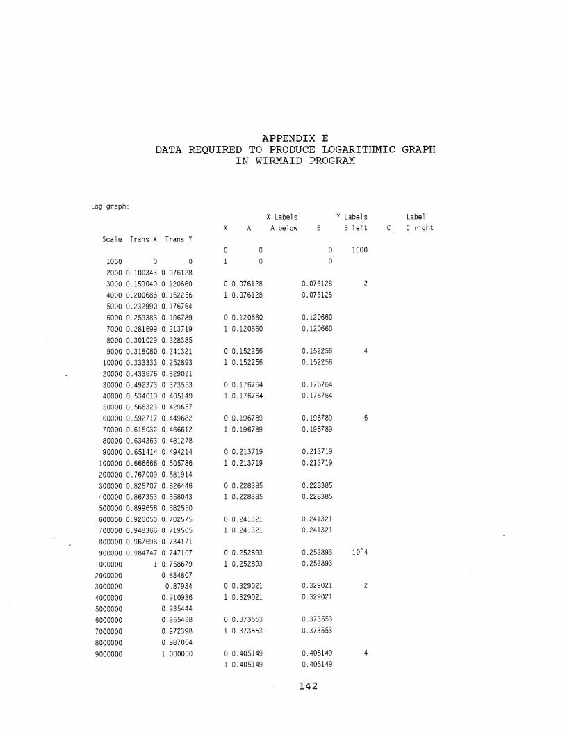
APPENDIX E DATA REQUIRED TO PRODUCE LOGARITHMIC GRAPH

IN WTRMAID PROGRAM

Log graph: X Label s Y Labels Label

X A A below B B left C C right

Scale Trans X Trans Y 0 0 0 1000

1000 0 0 1 0 0 2000 0.100343 0.076128 3000 0.159040 0.120660 o 0.076128 0.076128 2 4000 0.200686 0.152256 1 0.076128 0.076128 5000 0.232990 0.176764 6000 0.259383 0.196789 o 0.120660 0.120660 7000 0.281699 0.213719 1 0.120660 0.120660 8000 0.301029 0.228385 9000 0.318080 0.241321 o 0.152256 0.152256 4

10000 0.333333 0.252893 1 0.152256 0.152256 20000 0.433676 0.329021 30000 0.492373 0.373553 o 0.176764 0.176764 40000 0.534019 0.405149 1 0.176764 0.176764 50000 0.566323 0.429657 60000 0.592717 0.449682 o 0.196789 0.196789 6 70000 0.615032 0.466612 1 0.196789 0.196789 80000 0.634363 0.481278 90000 0.651414 0.494214 o 0.213719 0.213719

100000 0.666666 0.505786 1 0.213719 0.213719 200000 0.767009 0.581914 300000 0.825707 0.626446 o 0.228385 0.228385 400000 0.867353 0.658043 1 0.228385 0.228385 500000 0.899656 0.682550 600000 0.926050 0.702575 o 0.241321 0.241321 700000 0.948366 0.719505 1 0.241321 0.241321 800000 0.967696 0.734171 900000 0.984747 0.747107 o 0.252893 0.252893 10~4

1000000 1 0.758679 1 0.252893 0.252893 2000000 0.834807 3000000 0.87934 o 0.329021 0.329021 2

4000000 0.910936 1 0.329021 0.329021 5000000 0.935444 6000000 0.955468 o 0.373553 0.373553

7000000 0.972398 1 0.373553 0.373553

8000000 0.987064 9000000 1.000000 o 0.405149 0.405149 4

1 0.405149 0.405149

142

143

o 0.429657 0.429657 1 0.429657 0.429657

o 0.449682 0.449682 6 1 0.449682 0.449682

o 0.466612 0.466612 1 0.466612 0.466612

o 0.481278 0.481278 1 0.481278 0.481278

o 0.494214 0.494214 1 0.494214 0.494214

o 0.505786 0.505786 10-5

1 0.505786 0.505786

o 0.581914 0.581914 2 1 0.581914 0.581914

o 0.626446 0.626446 1 0.626446 0.626446

o 0.658043 0.658043 4 1 0.658043 0.658043

o 0.682550 0.682550 1 0.682550 0.682550

o 0.702575 0.702575 6 1 0.702575 0.702575

o 0.719505 0.719505 1 0.719505 0.719505

o 0.734171 0.734171 1 0.734171 0.734171

o 0.747107 0.747107 1 0.747107 0.747107

o 0.758679 0.758679 10'6 1 0.758679 0.758679

o 0.834807 0.834807 2 1 0.834807 0.834807

0 0.87934 0.87934 1 0.87934 0.87934

o 0.910936 0.910936 4 1 0.910936 0.910936

144

o 0.935444 0.935444 0.935444 0.935444

o 0.955468 0.955468 6 1 0.955468 0.955468

o 0.972398 0.972398 1 0.972398 0.972398

o 0.987064 0.987064 1 0.987064 0.987064

0 9

0 0 1000 0

0.100343 0 2 0.100343 1

0.159040 0 0.159040 1

0.200686 0 4 0.200686

0.232990 0 0.232990

0.259383 0 6 0.259383 1

0.281699 0 0.281699

0.301029 0 0.301029

0.318080 0 0.318080 1

0.333333 0 10'4

0.333333 1

0.433676 0 2 0.433676 1

0.492373 0 0.492373

0.534019 0 4 0.534019

145

0.566323 0 0.566323 1

0.592717 0 6 0.592717

0.615032 0 0.615032 1

0.634363 0 0.634363 1

0.651414 0 0.651414

0.666666 0 10'5

0.666666 1

0.767009 0 2

0.767009

0.825707 0 0.825707 1

0.867353 0 4 0.867353 1

0.899656 0 0.899656

0.926050 0 6 0.926050 1

0.948366 0 0.948366 1

0.967696 0 0.967696 1

0.984747 0 0.984747 1

0 10'6

X Y

G = 20 1800 34990 0.085090 0.390452

10000 114410 0.333333 0.520571

25000 144120 0.465980 0.545926

100000 274850 0.666666 0.616830 G=20

500000 900420 0.899656 0.747158

1000000 1770400 0.821414

G = 50

146

1800 34990 0.085090 0.390452 10000 114420 0.333333 0.520580 25000 150210 0.465980 0.550472

100000 304080 0.666666 0.627930 500000 1057150 0.899656 0.764783

1000000 2077750 1 0.838996 G=50 G = 80

1800 34990 0.085090 0.390452 10000 123540 0.333333 0.529003 25000 163900 0.465980 0.560051

100000 368570 0.666666 0.649055 500000 1373620 0.899656 0.793544 G=80

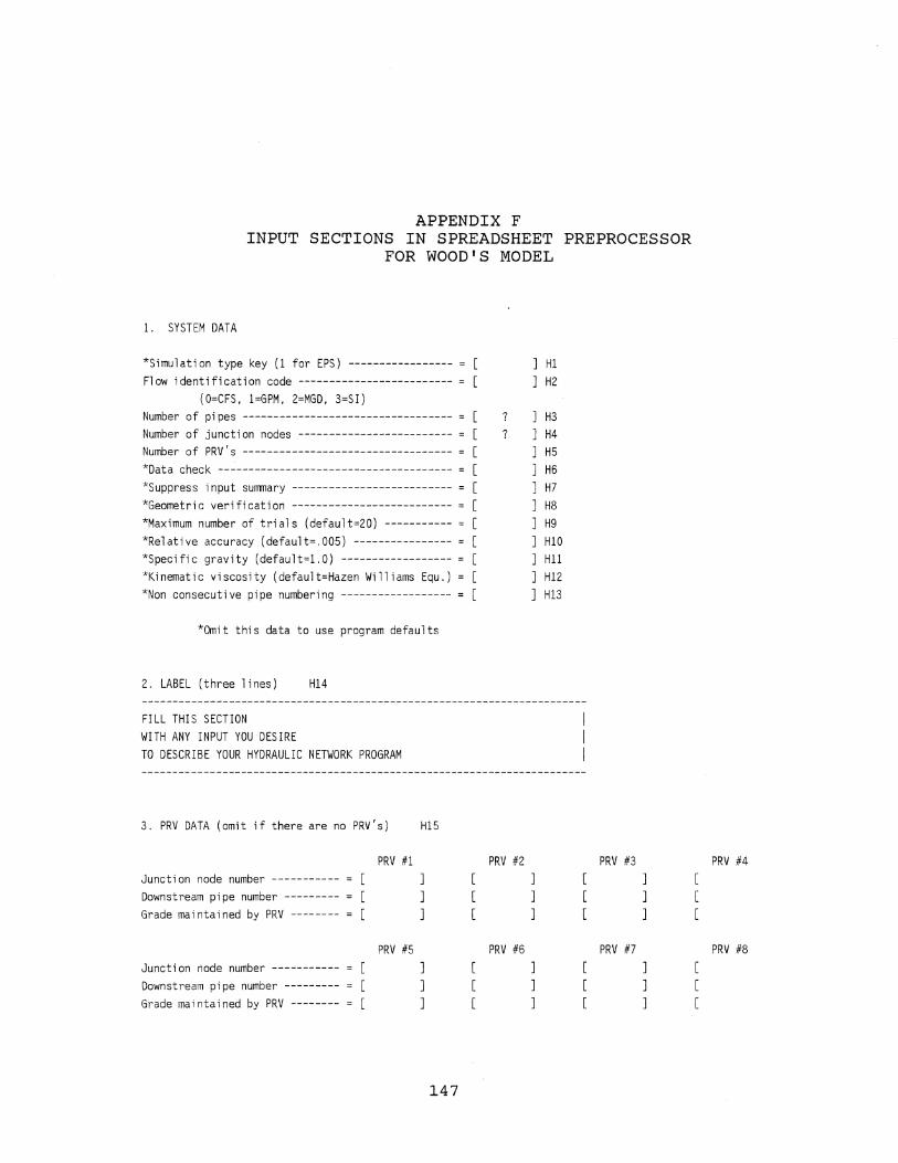
APPENDIX F INPUT SECTIONS IN SPREADSHEET PREPROCESSOR

FOR WOOD'S MODEL

1. SYSTEM DATA

*Simulation type key (1 for EPS) ----------------- = Flow identification code ------------------------- =

(O=CFS, l=GPM, 2=MGD, 3=51) Number of pipes ---------------------------------- = [ Number of junction nodes ------------------------- = [ Number of PRV's ---------------------------------- = [ *Data check -------------------------------------- = [ *Suppress input summary -------------------------- = [ *Geometric verification -------------------------- = [ *Maximum number of trials (default=20) ----------- = [ *Relative accuracy (default=.005) ---------------- = [ *Specific gravity (default=1.0) ------------------ = [ kKi nemati c vi scosity (defaul t=Hazen Wi 11 i ams Equ.) = [ *Non consecutive pipe numbering ------------------ = [

*Omit this data to use program defaults

2. LABEL (three lines) HI4

FILL THIS SECTION WITH ANY INPUT YOU DESIRE TO DESCRIBE YOUR HYDRAULIC NETWORK PROGRAM

3. PRV DATA (omit if there are no PRV's) HI5

PRV #1 Junction node number ----------- = ]

Downstream pipe number --------- = ]

Grade maintained by PRV -------- = ]

PRV #5 Junction node number ----------- = ]

Downstream pipe number --------- = ]

Grade maintained by PRV -------- = ]

147

HI H2

? ] H3 ? ] H4

] H5 ] H6 ] H7 ] H8 ] H9 ] HI0 ] Hll ] H12 ] H13

PRV #2 PRV #3 ] ]

] ]

] ]

PRV #6 PRV #7 ] ]

] ]

] ]

PRV #4

PRV #8

148

PRY #9 PRY #10 PRY #11 PRY #12 Junction node number ----------- = ] [ ] [ ] [

Downstream pipe number --------- = ] [ ] [ ] [

Grade maintained by PRY -------- = ] [ ] [ ] [

PRY #13 PRY #14 PRY #15 PRY #16 Junction node number ----------- = [ ] [ ] [ ] [ ]

Downstream pipe number --------- = [ ] [ ] [ ] [ ]

Grade maintained by PRY -------- = [ ] [ ] [ ] [ ]

PRY #17 PRY #18 PRY #19 PRY #20 Junction node number ----------- = [ ] [ ] [ ] [ ]

Downstream pipe number --------- = [ ] [ ] [ ] [ ]

Grade maintained by PRY -------- = [ ] [ ] [ ] [ ]

PRY #21 PRY #22 PRY #23 PRY #24 Junction node number ----------- = [ ] [ ] [ ] [ ]

Downstream pipe number --------- = [ ] [ ] [ ] [ ]

Grade maintained by PRY -------- = [ ] [ ] [ ] [ ]

PRY #25 PRY #26 PRY #27 PRY #28

Junction node number ----------- = [ ] [ ] [ ] [ ]

Downstream pipe number --------- = [ ] [ ] [ ] [ ]

Grade maintained by PRY -------- = [ ] [ ] [ ] [ ]

PRY #29 PRY #30 PRY #31 PRY #32

Junction node number ------~---- = [ ] [ ] [ ] [ ]

Downstream pipe number --------- = [ ] [ ] [ ] [ ]

Grade maintained by PRY -------- = [ ] [ ] [ ] [ ]

4. PIPE DATA H22

H16 H17 H18 Sum of Pipeline Node Node H21 Minor H23 H24 H25

Pipe Status Number Number H19 H2O Rough- Loss Pump FGN Pipe Number Code 1 2 Length Diameter ness Coef's Data HGL Number

? ? ? ? ?

2 2

3 3 4 4 5 5

5. PUMP DATA

Total number of pumps ---------- = ] H26

H27 Cutoff

Head Di scharge Head Di scharge Head Di scharge Pump

Number 1st 1st

2

3

4

5

Point

6. JUNCTION DATA

Point

o o o o o

H30

2nd 2nd Point Point

H29 Juncti on H31

3rd 3rd Point Point

H28 Ele- Node Pipes connecting this junction node Demand vation Number Pipe #1 Pipe #2 Pipe #3 Pipe #4 Pipe #5

8. OUTPUT OPTION DATA

2

3

4 5

Output selection --------------------------------- =

Number of juncts. for max-min pressure summary --- = Input next two items for limited output only

Number of pipes for limited output --------------- = Number of junction nodes for limited output ------ = Key for geometric data --------------------------- =

Changes incorporated prior to first run ---------- =

] ]

END OF ALL DATA ---------------------------------- = -2 ]

149

APPENDIX G HELP MESSAGES IN PREPROCESSOR FOR WOOD'S MODEL

1. Simulation Type Key Leave blank to run a regular simulation. Input the

number 1 to run an extended period simulation.

2. Flow Identification Code Leave blank for cubic feet per second. Input the number 1 for gallons per minute. Input the number 2 for million gallons per day. Input the number 3 for liters per second.

3. Number of Pipes Input the number of pipes in your network.

4. Number of Junction Nodes Input the number of junction nodes in your network.

5. Number of PRV's Input the number of pressure regulating valves in your

network. Leave blank if there are no pressure regulating valves in your network.

6. Data Check This option will allow the computer to read and check

all the input data including changes but suppresses the actual analysis.

output pertaining to the original data and changes is obtained and can be used for checking. This option is useful for checking physical data by hand before going to the expense of the analysis and is obtained at a fraction of the cost. It is also very useful for checking a number of changes before they are actually processed.

Input the number 1 to engage this option. Leave blank if this option is not desired.

7. Suppress Input Summary A complete summary of input data for pipelines and

junctions is normally output. However, this output can be redundant and lengthy and may be suppressed using this option.

Input the number 1 to engage this option. Leave blank if this option is not desired.

150

151

8. Geometric Verification The input data summary includes a list of pipes

connecting at each junction node which can be checked by the user against system geometry and, if verified, will assure that the input data for connecting nodes is correct. An option is available for computer verification of this data. If this option is used the computer will check pipes connecting junction nodes generated using the input data for this purpose. A successful check of this data will assure that the system is geometrically correctly input. A successful verification will produce a verifying message while an unsuccessful verification will produce a message identifying this error and the junction node where it occurred and will suppress the analysis until this discrepancy is removed.

Input the number 1 to engage this option. In addition, the within the junction section, the connecting pipes at each junction node must be input in ascending numerical order. Leave blank if this option is not desired.

9. Maximum Number of Trials This limit is set at 20 unless a different limit is

specified as the ninth number. It is unlikely that this limit will ever be reached, but it is imposed to guard against an unforeseen convergence problem (this conceivably could be caused by a check valve or a pump operating extremely close to its boundary condition).

Leave blank for default setting or input the number of trials you desire.

10. Relative Accuracy This parameter determines when the solution is

acceptable. It is defined as the total (absolute) change in flowrate in the pipes from the previous trial divided by the total (absolute) flowrate and is set at 0.005 unless this option is employed to change this value. It is unlikely that the user will want to exercise this option and change the relative accuracy and such a change is not recommended.

Leave blank for the default setting. Input another value to change the relative accuracy.

11. Specific Gravity Unless specified by the user, water is assumed to be

the liquid being transported. Leave blank if the default setting is desired. Input a

different specific gravity (ratio of liquid density to water density) if required.

152

12. Kinematic viscosity The default setting keys the use of the Hazen Williams

head loss equation, which is appropriate for water distribu­tion systems. For liquids (and for water, if desired) the Darcy Weisbach equation should be used.

Leave blank for the default setting. If the Darcy Weisbach equation is desired, input the value for the kinematic viscosity (in feet squared per second or meters squared per second for SI units). If this option is used, the pipe roughness for the expression must be input for the roughness within the pipe data section with the units of millifeet or millimeters for SI units.

13. Non Consecutive Pipe Numbering Non consecutive numbering junction nodes is always

acceptable. However, it is assumed that the pipes are numbered one to p, where p equals the total number of pipes, and the data is input in this order unless this option is employed.

Leave blank if consecutive numbering is used. Input the number 1 if you input pipes in a non consecutive order. In addition the pipes must be numbered in an ascending order. No alphabetic information is allowed.

14. Label Whatever is typed within this space appears as a

problem identification heading for the computer output.

15. PRV Data omit this section if pressure regulating valves are not

within your network. Note that for each PRV, the location of the PRV is defined by a junction node at the PRV and the pipe downstream from the PRV. In addition, the grade which the PRV is set to maintain, in feet or meters, is required. A total of 32 PRV's can be input.

16. Pipeline status Code Leave blank if there is no check valve in the pipe. Input the number 1 if there is a check valve in the

pipe. Input the number 2 if the pipe is closed.

17. Node Number 1 and Node Number 2 Input the two junction nodes which the pipe connects.

If the direction of flow is known, input the junction node number which the water is leaving as node number 1 and input the junction node which the water flows into as node number 2 .

153

18. Node Number 1 and Node Number 2 Input the two junction nodes which the pipe connects.

If the direction of flow is known, input the junction node number which the water is leaving as node number 1 and input the junction node which the water flows into as node number 2 .

19. Length Input the length of the pipe in feet or meters

depending on the units you have chose.

20. Diameter Input the inside diameter of the pipe in inches or

centimeters depending the units you have chosen.

21. Roughness Input"the Hazen Williams roughness coefficient if the

Hazen Williams head loss equation is being used. If the Darcy Weisbach head loss relationship is being used, then the pipe roughness in millifeet or millimeters is input here.

22. Sum of Minor Loss Coefficients Input the sum of the minor loss coefficients for this

pipe.

23. Pump Data Leave blank if no pump is in the line. Input the number -1 if a pump is in the line and you

desire to enter three pump operating data points within the pump section.

If you desire to enter the useful horsepower input by the pump, enter this value directly.

24. FGN HGL Leave blank if the pipe does not connect to a fixed

grade node. If the pipe connects to a fixed grade node, input the

value of the total grade (elevation + pressure head) in feet or meters.

25. Pipe Number Leave blank for consecutive numbering, 1,2,3 ... ,p. If non consecutive numbering is used, input pipe

number. Pipes must be in ascending order and no alphabetic information is allowed.

26. Total Number of Pumps Leave blank if no pumps are within the network.

Otherwise input the total number of pumps within the network.

154

27. Pump Data This data is supplied only for pumps described by

operating data. This option is keyed by a -1 for the pump data within the pipe data section. The head in feet or meters and the discharge in the flow units specified are included for three operating points. The first pump operating data point must be the cutoff head and discharge, the second point at an intermediate point of normal opera­tion, and the third point at the extreme end of normal pump operation. The pump data must be input in the same order as the pumps were listed in the pipe data section.

28. Demand Leave blank if there is no external demand at the node.

If there is an external demand at the junction node, input the value in the flow units specified. The value is positive for an outflow and negative for inflow.

29. Elevation Leave blank if you do not desire the pressure at this

node in the output data. Input the elevation in feet or meters if pressure output data is desired.

30. Junction Node Number Input the node number for this junction.

nodes are already numbered in this column but replaced by any number desired.

31. Pipes connecting This Junction Node

The junction they can be

Leave blank if you do not desire a geometric verifica­tion. If you asked for a geometric verification within the system data section, you must complete this section. Enter the number for each pipe connecting the junction node in ascending order.

32. Output option Data Leave this section blank. This section is for limiting

the amount of output data and for an extended period simulation. These cards have not been input into the Lotus 123 preprocessor at this time.

33. End of all Data An input of -2 indicates that all input has been

completed.

l. SYSTEM DATA

10

APPENDIX H DATA CARDS IN SPREADSHEET PREPROCESSOR

FOR WOOD'S MODEL

20 30 40 50 60 70 12345678901234567890123456789012345678901234567890123456789012345678901234567890

0 o ? ? 0 0 0 0 0 0.000000 0.00000 0.00000000 0 0

3. PRY DATA

10 20 30 40 50 60 70 12345678901234567890123456789012345678901234567890123456789012345678901234567890

0 0 0.00 0 0 0.00 0 0 0.00 0 0 0.00 0 0 0.00 0 0 0.00 0 0 0.00 0 0 0.00 0 0 0.00 0 0 0.00 0 0 0.00 0 0 0.00 0 0 0.00 0 0 0.00 0 0 0.00 0 0 0.00 0 0 0.00 0 0 0.00 0 0 0.00 0 0 0.00

4. PIPELINE DATA

10 20 30 40 50 60 70 12345678901234567890123456789012345678901234567890123456789012345678901234567890

o ? ? ? ? ? 0.00 0.00 0.00 0 0 0 0.00 0.00 0.00 0.00 0.00 0.00 2 0 0 0 0.00 0.00 0.00 0.00 0.00 0.00 3 0 0 0 0.00 0.00 0.00 0.00 0.00 0.00 4 0 0 0 0.00 0.00 - 0.00 0.00 0.00 0.00 5

5. PUMP DATA

10 20 30 40 50 60 70 1234567890123456789012345678901234567890123456789012345678901234567890123456789

0.00 0.00 0.00 0.00 0.00 0.00 0.00 0.00 0.00 0.00 0.00 0.00 0.00 0.00 0.00 0.00 0.00 0.00 0.00 0.00 0.00 0.00 0.00 0.00 0.00 0.00 0.00 0.00 0.00 0.00

155

156

6. JUNCTION DATA

10 20 30 40 50 60 70 12345678901234567890123456789012345678901234567890123456789012345678901234567890

0.00 0.00 1 0 0 0 0 0 0 0 0 0 0 0.00 0.00 2 0 0 0 0 0 0 0 0 0 0 0.00 0.00 3 0 0 0 0 0 0 0 0 0 0 0.00 0.00 4 0 0 0 0 0 0 0 0 0 0 0.00 0.00 5 0 0 0 0 0 0 0 0 0 0

7. BLANK LINE

0

8. OUTPUT OPTION DATA

10 20 30 40 50 60 70 12345678901234567890123456789012345678901234567890123456789012345678901234567890

o 0 0 0 0 0

END OF CHANGES - END OF ALL DATA

10 20 30 40 50 60 70 12345678901234567890123456789012345678901234567890123456789012345678901234567890

-2.000

APPENDIX I MACROS IN SPREADSHEET PRE- AND POSTPROCESSORS

FOR WOOD'S MODEL

Macro in Preprocessor

\m {menuca 11 menu} SECTIONS COMPILE COPY HELP QUIT CHANGES Moves theInitiatesMakes a cProvides Ends progCopies existing file onto this diskette so that change {menucal 1 {branch c{goto}eol{menucall/qy {goto}exl-{?}-{home}/wgpd/fcce{?}-{goto}fgl-{?}-{home}

{menucall sections} SYSTEM LABEL PRY PIPE PUMP JUNCTION OUTPUT Moves theMoves theMoves theMoves theMoves theMoves theMoves the cursor to this section. {goto}sys{goto}lab{goto}prv{goto}pip{goto}pum{goto}jun{goto}output-{quit} {quit} {quit} {quit} {quit} {quit} {quit}

{menucall help} SYSTEM I-SYSTEM 9-LABEL PRY PIPE I6-2PIPE 24-2PUMP JUNCTION OUTPUT Provides Provides Provides Provides Provides Provides Provides Provides Provides help in this secti {menucal 1 {menucall {goto}14-{goto}IS-{menucal 1 {menucall {menucal 1 {menucal 1 {menucall system}

{menuca 11 sys} 1 2

{?} {?}

{goto}lab{goto}prv­{quit} {quit}

3 4 S 6 7 8

Provides Provides Provides Provides Provides Provides Provides Provides further explanation of this {goto}l- {goto}2- {goto}3- {goto}4- {goto}S- {goto}6- {goto}7- {goto}8-{?} {?} {?} {?} {?} {?} {?} {?} {goto}sys{goto}sys{goto}sys{goto}sys{goto}sys{goto}sys{goto}sys{goto}system­{quit} {quit} {quit} {quit} {quit} {quit} {2quit} {quit}

{menuca11 sysl} 9 10 11 12 13 Provides Provides Provides Provides Provides further explanation of this data entry point. {goto }g- {goto }lo-{goto} 11-{goto} 12-{goto} 13" {?} {?} {?} {?} {?}

{goto}sys{goto}sys{goto}sys{goto}sys{goto}system­{quit} {quit} {quit} {quit} {quit}

157

{menuca11 pip} 16 17 18 19 20 21 22 23 Provides Provides Provides Provides Provides Provides Provides Provides further explanation of this {goto}16-{goto}17-{goto}18-{goto}19-{goto}20-{goto}21-{goto}21-{goto}23-{?} {?} {?} {?} {?} {?} {?} {?}

{goto}pip{goto}pip{goto}pip{goto}pip{goto}pip{goto}pip{goto}pip{goto}pipe­{quit} {quit} {quit} {quit} {quit} {quit} {quit} {quit}

{menuca 11 pi pI} 24 25 Provides Provides further explanation of this data entry point. {goto}24-{goto}25-{?} {?}

{goto}pip{goto}pipe­{quit} {quit}

{menucall pup} 26 27 Provides Provides further explanation of this data entry point. {goto}26-{goto}27-{?} {?} {goto}pum{goto}pump­{quit} {quit}

{menuca 11 j un} 28 29 30 31 Provides Provides Provides Provides further explanation of this data entry point. {goto}28-{goto}29-{goto}30-{goto}31-{?} {?} {?} {?}

{goto}jun{goto}jun{goto}jun{goto}junction­{quit} {quit} {quit} {quit}

{branch compile} /wgpd /fdb:-{goto}w1-/fcceblank-/wgra{goto}g26-{edit}­/pfsystem-rrw6.aj6-omlO-mtO-ouqgq /pflabel-rra63.h65-omlO-mtO-ouqgq {goto}cr6-{end}{right}{down g28} /re{end}{left}{end}{down}-/pfprv"rrcr6 .dc13'· oml O-mtO·ouqgq {goto}a16-{end}{right}{down g26} /re{end}{left}{end}{down}-{goto}al 6-/rv{end}{right}{end}{down}-al 1000-{goto}as1000-{if e323>0}{for ef13.1.g26.1.mac_rtn} /pfpipe-rral1000,au1100-omlO-mtO-ouqgq {goto}aw6-{end}{right}{down e323} /re{ end}{l eft} {end}{ down},­/pfpump-rraw6.bbl05-omlO-mtO-ouqgq

macro description

disable protection combines file BLANK creates system print file creates label print file creates prv file

moves pipe file

{if @cellinserts blank rows {down}{recreates pipe print file

creates pump print file

158

{goto}bg6-{end}{right}{down g27} /re{end}{left}{end}{down}­/pfjunction-rrbg6.bslOS-omlO-mtO-ouqgq /pfoutput-rrbu6.ce6-omlO-mtO-ouqgq /pfend-rrch6.cm6-omlO-mtO-ouqgq /pfblank-rrbull-omlO-mtO-ouqgq {goto}a700-/fitsystem-{down}{goto}a701-/fitlabel-{goto}a704-

{if g28>O}/fitprv-{goto}alOOO-{end}{up}{down} /fitpipe-{goto}alOOO-{end}{up}{down} {if e323>O}/fitpump-{goto}alOOO-{end}{up}{down} /fitjunction-{end}{down}{down} /fitblank-{down} /fitoutput-{down} /fitend-{if e323>O}{goto}a700-{down g26+e323+3+g28+e323} {for eg36.1.e323.1.sub_rtn} {i f e323>O}{down} /wdr{end}{down}{up}" {goto}eol-{?}-/pf{?}-ra700.mlOOO-omlO-mtO-ouqgq /qy

Macro in Postprocessor

\m {menuca 11 menu}

IMPORT COPY HELP QUIT

InitiatesProduces An explanTerminates the program. {branch i/fdb:-/fs/rnchere-/qy

{branch import} /wgpd{goto}bblOO-{?}-{goto}ccl-/fin{?}­{goto}cc2000-{end}{up}{up}/c{down}-akl­{end}{up}{end}{up}/c{end}{down}{right}-v6-{end}{up}/c-tC {end}{up}{end}{up}!c{end}{down}{end}{right}-k4-{end}{up}{end}{up}/c{end}{down}{end}{right}-a4-{goto}a2000-{end}{up}{down 3}/ckl.olOO-­{goto}a2000-{end}{up}{down 3}/cql.tl-­{goto}a2000-{end}{up}{down 3}/cvl.wlOO-­{goto}a2000-{end}{up}{down 3}/cadl.ak2-­/rekl.aklOO-/reccl.cz2000-{goto}a4-/wdr-{home} {quit}

creates junction print file

creates output print file creates end print file creates blank print file moves cursor imports system print file imports label print file

imports pry print file if it exists imports pipe print file moves cursor imports pump file if it exists imports juntion print file imports blank print file imports output print file imports end print file inserts pump file data within pipe f

/m-{end}{up}{up}-{ {return} deletes b

saves fil e quit

macro description

imports file to postprocess configures net flow data configures fixed grade node summary data configures net system demand figure configures data configures flow and velocity data configures data configures net system demand figure configures fixed grade node summary data configures net flow data clears spreadsheet return to home quit

159

REFERENCES

Bradley, S. P., A. C. Hax, and T. L. Magnanti. 1977. Applied Mathematical Programming, Addison Wesley Publishing Company, Reading, Massachusetts.

Calise, S. J., G. S. Walters, and D. T. Zimmer. 1984. Microcomputers and Software Provide Useful Tools for Sewer System Evaluation, Public Works, Vol. 115, No. 7, 61-62.

Cesario L. 1984. Network Analysis Survey, Computer Assisted Design of Water Systems Committee, American Water Works Association, Denver, Colorado.

Cullen, M. and M. Murrell. 1985. Developments in Sewer Management Information Systems, Civil Engineering, Vol. 44, No.8, 25-29, 50.

Fine, E. S. 1987. Plotting Logarithmic Graphs in 1-2-3, Lotus, Vol. 3, No.3, 71-75.

Gregory, W. H. 1986. Lotus, Lotus Publishing Corporation, Cambridge, Massachusetts.

Gumerman, R. C., R. L. Culp, and S. P. Hansen. 1979. Estimating Water Treatment Costs, Volume 2, Cost Curves Applicable to 1 to 200 mgd Treatment Plants, Municipal Environmental Research Laboratory, Office of Research and Development, U.S. Environmental Protection Agency, Cincinnati, Ohio, EPA-600j2-79-162b, August 1979.

Hancock, M. C. 1986. Analysis of Water Resources Problems Using Electronic Spreadsheets, M. S. Thesis, University of Florida, Gainesville.

Harris, R. U. 1984. Computer Modeling in Water System Planning and Design, Journal of American Water Works Association, Vol. 76, No.7, 78-81.

Heenan, W. A. and R. W. Serth. 1986. Detecting Errors in Process Data, Chemical Engineering, Vol. 32, 99-103.

160

161

Hillier, F. S. and G. J. Lieberman. 1967. Introduction to Operations Research, Fourth Edition, Holden-Day, Inc., Oakland, California.

Iordaache, c., R. S. H. Mah, and A. C. Tamhane. 1985. Performance Studies of the Measurement Test for Detection of Gross Errors in Process Data, AIChE J., Vol. 31, 1187-1194.

Johnson, L. E. 1986. Journal of Water Resources Planning and Management (ASCE), Vol. 112, No.3, 308-325.

Koh, Eng Seng and D. R. Maidment. 1984. Microcomputer Programs for Designing Water Systems, Journal American Water Works Association, Vol. 76, No.7, 62-65.

LeBlond, G. T. and D. F. Cobb. 1985. Using 1-2-3, 2nd Edition, Que Corporation, Indianapolis, Indiana.

Lotus Development Corporation. 1985. 123 Reference Manual, Release 2, Second Printing, Cambridge, Massachusetts.

Mah, R. S. H., G. M. Stanley, and D. Dowing. 1976. Reconciliation and Rectification of Process Flow and Inventory Data, Industrial Engineering Chemistry, Process Description and Developments, Vol. 15, 175-183.

Mah, R. S. H. and A. C. Tamhane. 1982. Detection of Gross Errors in Process Data, AIChE J., Vol 28, 828-830.

Miles, S. W. and J. P. Heaney. 1986. Application of a Lotus Spreadsheet for a SWMM Preprocessor, Proceedings of Stormwater and Water Quality Model USERS Group Meeting, March 24-25, Orlando, Florida, EPA/600/9-86/023.

Ridington, R. W. Jr. and M. M. Williams. 1985. The Hidden Power of Lotus 1-2-3: Using Macros, Brady Communica­tions Company, Inc., Bowie, Maryland.

Schrage, L. 1984. Linear, Integer, and Quadratic Programming with Lindo, The Scientific Press, Palo Alto, California.

Serth, R. W. and W. A. Hennan. 1986. Gross-Error Detection and Data Reconciliation in steam-Metering Systems, AIChEJ, Vol 32, 733-742.

Smith, R. 1986. Computer Assisted Preliminary Design for Drinking Water Treatment Process Systems, Water Engineering Research Laboratory, U. S. Environmental Protection Agency, Cincinnati, Ohio, EPA/600/S2-86/007.

Viessman, W. Jr. and M. J. Hammer. 1985. Water Supply and Pollution Control, Fourth Edition, Harper & Row, Publishers, New York.

Wood, Don J. 1980. User's Manual: Computer Analysis of Flow in Pipe Networks Inculding Extended Period Simulation, Office of Continuing Education and Extension, College of Engineering, University of Kentucky, Lexington.

162

BIOGRAPHICAL SKETCH

Captain Michael A. Moore was born on January 17, 1955,

in Jacksonville, Florida, to Rear Admiral and Mrs. V. W.

Moore, Jr. He attended numerous public schools in

conjunction with his father's assignments with the U.S. Navy

and graduated from Camp Zama American High School in Japan.

He enrolled in the Army Reserve Officer Training Corps

program at the University of California, Santa Barbara, and

received his commission and a Bachelor of Arts degree in

environmental science in 1978.

He has served tours at the Air Defense Artillery Basic

Officer Course at Fort Bliss, Texas, with the Second

Battalion, 67th Air Defense Artillery in Germany, at the

Engineer Officer Advanced Course at Fort Belvoir, Virginia,

and with the 14th Engineer Battalion (Combat, Corps) at Fort

Ord, California. In 1985 he was assigned to the University

of Florida, Gainesville, and entered the Department of

Environmental Engineering Sciences graduate program with a

concentration in water resource analysis. He received a

Master of Science degree in August, 1987. His next assign­

ment will be with the Middle East-Africa Project Office,

U.S. Army Corps of Engineers with duty station in Cairo,

Egypt.

163