analysis of transient electromagentic …lipeijun/paper/2015/lww_siap_2015.pdf · siam j. appl....

SIAM J. APPL. MATH. c© 2015 Society for Industrial and Applied MathematicsVol. 75, No. 4, pp. 1675–1699

ANALYSIS OF TRANSIENT ELECTROMAGENTIC SCATTERINGFROM A THREE-DIMENSIONAL OPEN CAVITY∗

PEIJUN LI† , LI-LIAN WANG‡ , AND AIHUA WOOD§

Abstract. This paper is concerned with the mathematical analysis of the time-domain Maxwellequations in a three-dimensional open cavity. An exact transparent boundary condition is developedto reformulate the open cavity scattering problem in an unbounded domain, equivalently, into aninitial-boundary value problem in a bounded domain. The well-posedness and stability are studiedfor the reduced problem. Moreover, an a priori estimate is established for the electric field with aminimum regularity requirement for the data.

Key words. time-domainMaxwell equations, transparent boundary conditions, three-dimensionalopen cavity scattering problem, well-posedness, stability, a priori estimates

AMS subject classifications. 35Q61, 78A25, 78M30

DOI. 10.1137/140989637

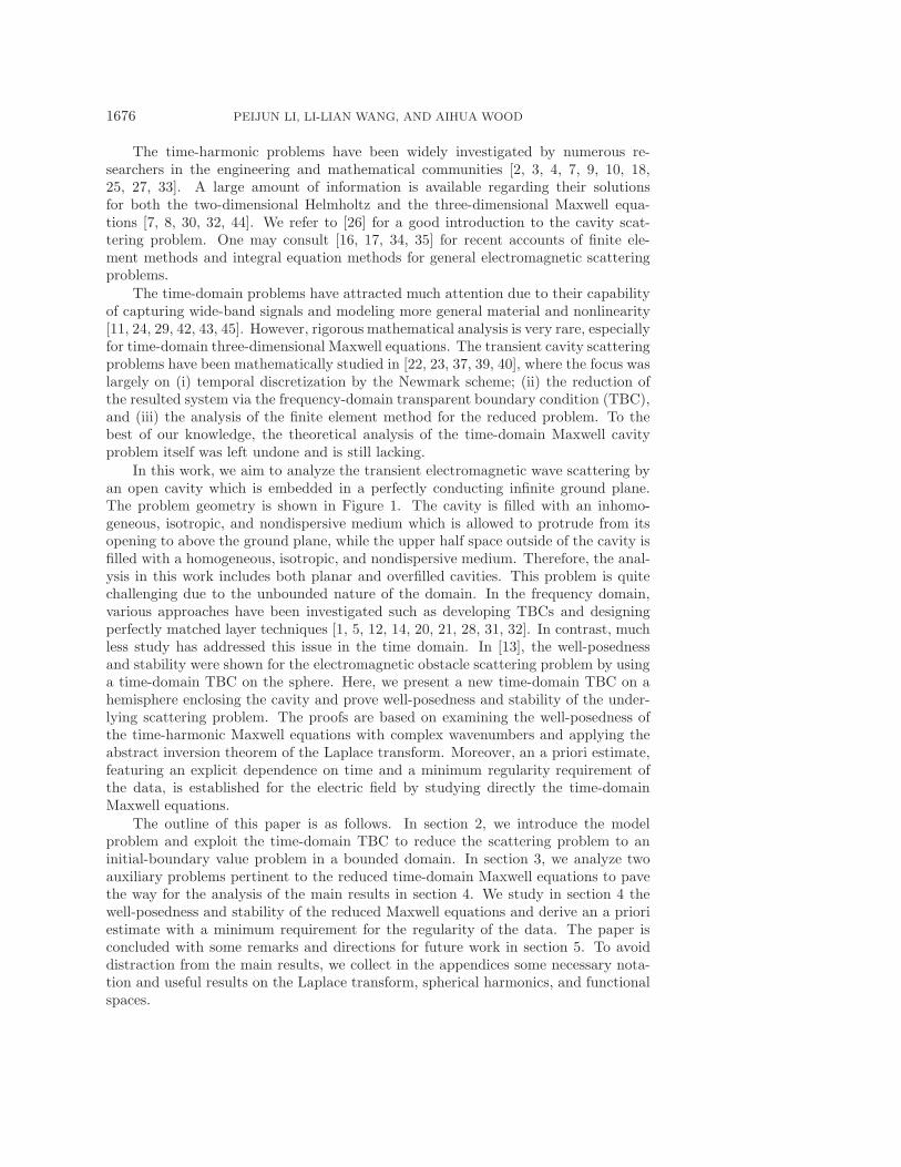
1. Introduction. This paper is concerned with the mathematical analysis ofan electromagnetic open cavity scattering problem where the wave propagation isgoverned by the time-domain Maxwell equations. As shown in Figure 1, an opencavity refers to a compactly supported domain with its opening aligned with the infi-nite ground plane. Cavity scattering problems have significant industry and militaryapplications such as the design of cavity-backed conformal antennas and deliberatecontrol in the form of enhancement or reduction of a radar cross section.

S

Γ+R

n

n

n

eρ

Γg Γg

D

B+R

Ωe

Fig. 1. A schematic diagram of the open cavity problem geometry.

∗Received by the editors September 30, 2014; accepted for publication (in revised form) June 1,2015; published electronically August 4, 2015.

http://www.siam.org/journals/siap/75-4/98963.html†Department of Mathematics, Purdue University, West Lafayette, IN 47907 (lipeijun@math.

purdue.edu). This author’s research was supported in part by NSF grant DMS-1151308.‡Division of Mathematical Sciences, School of Physical and Mathematical Sciences, Nanyang

Technological University, 637371, Singapore ([email protected]). This author’s research was partiallysupported by Singapore MOE AcRF Tier 1 grant (RG 15/12), MOE AcRF Tier 2 grant (MOE 2013-T2-1-095, ARC 44/13), and Singapore A∗STAR-SERC-PSF grant (122-PSF-007).

§Department of Mathematics and Statistics, Air Force Institute of Technology, WPAFB, OH45433 ([email protected]). This author’s research was supported in part by AFOSR grantsF1ATA02059J001 and F1ATA01103J001.

1675

http://www.siam.org/journals/siap/75-4/98963.html

mailto:[email protected]




1676 PEIJUN LI, LI-LIAN WANG, AND AIHUA WOOD

The time-harmonic problems have been widely investigated by numerous re-searchers in the engineering and mathematical communities [2, 3, 4, 7, 9, 10, 18,25, 27, 33]. A large amount of information is available regarding their solutionsfor both the two-dimensional Helmholtz and the three-dimensional Maxwell equa-tions [7, 8, 30, 32, 44]. We refer to [26] for a good introduction to the cavity scat-tering problem. One may consult [16, 17, 34, 35] for recent accounts of finite ele-ment methods and integral equation methods for general electromagnetic scatteringproblems.

The time-domain problems have attracted much attention due to their capabilityof capturing wide-band signals and modeling more general material and nonlinearity[11, 24, 29, 42, 43, 45]. However, rigorous mathematical analysis is very rare, especiallyfor time-domain three-dimensional Maxwell equations. The transient cavity scatteringproblems have been mathematically studied in [22, 23, 37, 39, 40], where the focus waslargely on (i) temporal discretization by the Newmark scheme; (ii) the reduction ofthe resulted system via the frequency-domain transparent boundary condition (TBC),and (iii) the analysis of the finite element method for the reduced problem. To thebest of our knowledge, the theoretical analysis of the time-domain Maxwell cavityproblem itself was left undone and is still lacking.

In this work, we aim to analyze the transient electromagnetic wave scattering byan open cavity which is embedded in a perfectly conducting infinite ground plane.The problem geometry is shown in Figure 1. The cavity is filled with an inhomo-geneous, isotropic, and nondispersive medium which is allowed to protrude from itsopening to above the ground plane, while the upper half space outside of the cavity isfilled with a homogeneous, isotropic, and nondispersive medium. Therefore, the anal-ysis in this work includes both planar and overfilled cavities. This problem is quitechallenging due to the unbounded nature of the domain. In the frequency domain,various approaches have been investigated such as developing TBCs and designingperfectly matched layer techniques [1, 5, 12, 14, 20, 21, 28, 31, 32]. In contrast, muchless study has addressed this issue in the time domain. In [13], the well-posednessand stability were shown for the electromagnetic obstacle scattering problem by usinga time-domain TBC on the sphere. Here, we present a new time-domain TBC on ahemisphere enclosing the cavity and prove well-posedness and stability of the under-lying scattering problem. The proofs are based on examining the well-posedness ofthe time-harmonic Maxwell equations with complex wavenumbers and applying theabstract inversion theorem of the Laplace transform. Moreover, an a priori estimate,featuring an explicit dependence on time and a minimum regularity requirement ofthe data, is established for the electric field by studying directly the time-domainMaxwell equations.

The outline of this paper is as follows. In section 2, we introduce the modelproblem and exploit the time-domain TBC to reduce the scattering problem to aninitial-boundary value problem in a bounded domain. In section 3, we analyze twoauxiliary problems pertinent to the reduced time-domain Maxwell equations to pavethe way for the analysis of the main results in section 4. We study in section 4 thewell-posedness and stability of the reduced Maxwell equations and derive an a prioriestimate with a minimum requirement for the regularity of the data. The paper isconcluded with some remarks and directions for future work in section 5. To avoiddistraction from the main results, we collect in the appendices some necessary nota-tion and useful results on the Laplace transform, spherical harmonics, and functionalspaces.

TRANSIENT ELECTROMAGNETIC SCATTERING 1677

2. Formulation and reduction of the problem. In this section, we intro-duce the mathematical model of interest and exploit the exact TBC to reduce theunbounded domain to a bounded one.

2.1. A model problem. We describe the setting of the cavity problem anddefine some necessary notation. As seen in Figure 1, denote by D the cavity embeddedin the perfectly electrically conducting infinite ground plane Γg. Let S = ∂D∩R3

−, thepart of cavity wall below the ground, be Lipschitz continuous and perfectly electricallyconducting. The medium in the cavity is characterized by the dielectric permittivityε and the magnetic permeability μ, which satisfy

0 < εmin ≤ ε ≤ εmax < ∞, 0 < μmin ≤ μ ≤ μmax < ∞.

Here εmin, εmax, μmin, and μmax are constants. Let B+R and Γ+

R be the half-ball andhemisphere above the ground plane, where the radius R is large enough to completelycontain the possibly overfilled portion of the cavity. The unbounded region R3

+ \ B+R

is filled with a homogeneous, isotropic, and nondispersive medium with a constantpermittivity ε0 and a constant permeability μ0. Throughout this paper, we assumefor simplicity in exposition that ε0 = μ0 = 1. Finally, we denote by Ω = B+

R ∪ Dthe bounded domain in which our reduced initial-boundary value problem will beformulated. It is easy to note that ∂Ω = Γ+

R ∪ S is Lipschitz continuous.As is shown in Figure 1, it is evident that the problem geometry is applicable not

only to the open cavity problem but also to a broader class of scattering problemswhere the surface S or a part of it may be above the ground plane.

Consider the system of time-domain Maxwell equations in R3+ ∪D for t > 0:

(2.1)

{∇×E(r, t) + μ∂tH(r, t) = 0,

∇×H(r, t)− ε∂tE(r, t) = J(r, t),

where r = (x, y, z) ∈ R3, E is the electric field, H is the magnetic field, and J isthe electric current density which is assumed to be compactly supported in D. Thesystem is constrained by the initial conditions:

(2.2) E |t=0 = E0, H |t=0 =H0 in R3+ ∪D,

where E0 and H0 are also assumed to be compactly supported in D. We considerthe perfectly electrical conducting boundary condition on the ground plane and cavitywall:

(2.3) n×E = 0 on Γg ∪ S, t > 0,

where n is the unit outward normal vector on Γg ∪ S. In addition, we impose theSilver–Muller radiation condition:

(2.4) r × (∂tE × r) + r × ∂tH = o(|r|−1), as |r| → ∞, t > 0,

where r = r/|r|.The purpose of this paper is to study the well-posedness and establish the stability

for the time-domain electromagnetic cavity scattering problem (2.1)–(2.4). Hereafter,the expression “a � b” stands for a ≤ Cb, where C is a generic positive constantindependent of any function and important parameters, which are clear from thecontext.


2.2. Transparent boundary condition. We introduce a TBC to reformulatethe electromagnetic wave propagation problem into an equivalent initial-boundaryvalue problem in a bounded domain. The essential idea is to design a boundaryoperator which maps the tangential component of the electric field to the tangentialtrace of the magnetic field.

More precisely, we consider the reduced initial-boundary value problem:

(2.5)

⎧⎪⎪⎪⎪⎪⎨⎪⎪⎪⎪⎪⎩

∇×E + μ∂tH = 0, ∇×H − ε∂tE = J in Ω, t > 0,

E |t=0 = E0, H |t=0 =H0 in Ω,

n×E = 0 on S, t > 0,

T [EΓ+R] =H × n on Γ+

R, t > 0,

where EΓ+Ris the tangential trace of E on Γ+

R, and T is the time-domain electric-to-

magnetic (EtM) Calderon operator, as the counterpart of the time-harmonic setting,for instance, with a spherical boundary (cf. [17, 34]).

In what follows, we derive the formulation of the operator T and analyze itsimportant properties. Equivalently, we aim to prove the well-posedness and stabilityof the reduced problem (2.5). In particular, an a priori estimate is established witha minimum requirement for the regularity of the data. The proofs are based on theabstract inversion theorem of the Laplace transform and the a priori estimates forthe time-harmonic Maxwell equations with a complex wavenumber. These will be themain topics of the forthcoming sections.

Since J is supported in D and ε0 = μ0 = 1, the Maxwell equations (2.1) become

(2.6) ∇×E + ∂tH = 0, ∇×H − ∂tE = 0 in Ωe := R3+ \ B+

R , t > 0.

Let E(r, s) = L (E) and H(r, s) = L (H) be the Laplace transforms of E(r, t) andH(r, t) with respect to t, respectively, where the complex variable

(2.7) s = s1 + is2 with s1, s2 ∈ R, s1 > 0, i =√−1 ,

as seen in Appendix A. Recall that

L (∂tE) = sE −E0, L (∂tH) = sH −H0.

Taking the Laplace transform of (2.6), and noting that E0,H0 are supported in D,we obtain the time-harmonic Maxwell equations with complex parameters:

(2.8) ∇× E + sH = 0, ∇× H − sE = 0 in Ωe, s1 > 0.

Let h(1)n (z) be the spherical Hankel function of the first kind of order n (cf. [41]).

We introduce the vector wave functions

(2.9)

{Mm

n (ρ, θ, ϕ) = ∇× (rh(1)n (isρ)Xm

n (θ, ϕ)),

Nmn (ρ, θ, ϕ) = −s−1∇×Mm

n (θ, ϕ),

where (ρ, θ, ϕ) is the spherical coordinates, and Xmn is the rescaled spherical harmonic

function defined in (B.2). We refer to Appendix B for the properties of sphericalharmonics and the relevant calculus to be used throughout this paper.


The vector wave functions in (2.9) are the radiation solutions of (2.8) in R3 \ {0}(cf. [34, Theorem 9.16]):

(2.10) ∇×Mmn (ρ, θ, ϕ)+ sNm

n (ρ, θ, ϕ) = 0, ∇×Nmn (ρ, θ, ϕ)− sMm

n (ρ, θ, ϕ) = 0.

It can be verified from (2.9) that the vector wave functions satisfy

(2.11) Mmn (ρ, θ, ϕ) = h(1)

n (isρ)∇ΓXmn (θ, ϕ) × eρ

and

Nmn (ρ, θ, ϕ) = −

√n(n+ 1)

sρ

(h(1)n (isρ) + isρ(h(1)

n )′(isρ))Xm

n (θ, ϕ)

−n(n+ 1)

sρh(1)n (isρ)Y m

n (θ, ϕ)eρ.(2.12)

Once again, we refer to Appendix B for the notation and definition. A simple calcu-lation yields{

eθ ×Mmn (ρ, π/2, ϕ) = 0 for |m| ≤ n, m+ n = even, n ∈ N,

eθ ×Nmn (ρ, π/2, ϕ) = 0 for |m| ≤ n, m+ n = odd, n ∈ N.

Therefore, in the domain Ωe, the solution of the electric field E(ρ, θ, ϕ, s), which

satisfies the perfectly electric conducting condition n × E = 0 on Γg, i.e., eθ ×E(ρ, π/2, ϕ, s) = 0, can be written in the series

(2.13) E(ρ, θ, ϕ, s) =

odd∑|m|≤n

αmn (s)Nm

n (ρ, θ, ϕ) +

even∑|m|≤n

βmn (s)Mm

n (ρ, θ, ϕ),

which is uniformly convergent on compact subsets in Ωe. The corresponding magneticfield H is given by

(2.14) H = −s−1∇× E = −odd∑

|m|≤n

αmn (s)Mm

n (ρ, θ, ϕ) +

even∑|m|≤n

βmn (s)Nm

n (ρ, θ, ϕ).

Note that in the above, we compressed the summation notation as in Appendix B.To deduce the explicit representation of the EtM Calderon operator, we need to

express EΓ+R= −eρ× (eρ× E) and H ×eρ on Γ+

R in terms of the coefficients αmn and

βmn . From the definition (2.11), one verifies that

−eρ × (eρ ×Mmn (ρ, θ, ϕ)) = −

√n(n+ 1)h(1)

n (isρ)Y mn (θ, ϕ),

−eρ × (eρ ×Nmn (ρ, θ, ϕ)) = −

√n(n+ 1)

sρ

(h(1)n (isρ) + isρ h(1)

n

′(isρ)

)Xm

n (θ, ϕ),

and

eρ ×Mmn (ρ, θ, ϕ) =

√n(n+ 1)h(1)

n (isρ)Xmn (θ, ϕ),

eρ ×Nmn (ρ, θ, ϕ) = −

√n(n+ 1)

sρ

(h(1)n (isρ) + isρ h(1)

n

′(isρ)

)Y m

n (θ, ϕ).


Therefore, by (2.13), the tangential component of the electric field along Γ+R is

EΓ+R= −

odd∑|m|≤n

√n(n+ 1)

sR

(h(1)n (isR) + isR h(1)

n

′(isR)

)αmn (s)Xm

n (θ, ϕ)

+

even∑|m|≤n

√n(n+ 1)h(1)

n (isR)βmn (s)Y m

n (θ, ϕ),

and similarly, by (2.14), the tangential trace of the magnetic field along Γ+R is

H × eρ =

odd∑|m|≤n

√n(n+ 1)h(1)

n (isR)αmn (s)Xm

n (θ, ϕ)

+

even∑|m|≤n

√n(n+ 1)

sR

(h(1)n (isR) + isRh(1)

n

′(isR)

)βmn (s)Y m

n (θ, ϕ).

Consequently, we have the following explicit representation of the frequency do-main EtM Calderon operator B: given any tangential component of the electric fieldalong Γ+

R with the expansion

(2.15) u =

odd∑|m|≤n

αmn X

mn +

even∑|m|≤n

βmn Y

mn ,

the tangential trace of the magnetic field on Γ+R is

(2.16) B[u] = −odd∑

|m|≤n

sR

1 + r(1)n (isR)

αmn X

mn −

even∑|m|≤n

(1 + r(1)n (isR))

sRβmn Y

mn ,

where

(2.17) r(1)n (z) =z h

(1)n

′(z)

h(1)n (z)

.

We now analyze some properties of the EtM Calderon operator and refer toAppendix D for the definitions of the function spaces to be used hereafter.

Lemma 2.1. The Calderon operator B : H−1/2(curl, Γ+R) → H−1/2(div, Γ+

R) iscontinuous.

Proof. For any u,v ∈H−1/2(curl, Γ+R), we can expand

u =

odd∑|m|≤n

um1nX

mn +

even∑|m|≤n

um2n Y

mn , v =

odd∑|m|≤n

vm1nXmn +

even∑|m|≤n

vm2n Ymn .

Then we have from (2.16) that

B[u] = −odd∑

|m|≤n

sR um1n

1 + r(1)n (isR)

Xmn −

even∑|m|≤n

(1 + r(1)n (isR))um

2n

sRY m

n .


To prove the lemma, it is required to estimate

(2.18) 〈B[u],v〉 = −odd∑

|m|≤n

sR

1 + r(1)n (isR)

um1n v

m1n −

even∑|m|≤n

(1 + r(1)n (isR))

sRum2n v

m2n.

It follows from the Cauchy–Schwarz inequality that

|〈B[u],v〉| ≤⎡⎣ odd∑|m|≤n

√1 + n(n+ 1)

|1 + r(1)n (isR)|2

|sR|2 |um1n|2 +

even∑|m|≤n

|1 + r(1)n (isR)|2√

1 + n(n+ 1)

|um2n|2

|sR|2

⎤⎦1/2

×⎡⎣ odd∑|m|≤n

1√1 + n(n+ 1)

|vm1n|2 +even∑

|m|≤n

√1 + n(n+ 1)|vm2n|2

⎤⎦1/2

.

By Lemma C.3, we have√1 + n(n+ 1)

|1 + r(1)n (isR)|2

|sR|2 |um1n|2 =

1√1 + n(n+ 1)

1 + n(n+ 1)

|1 + r(1)n (isR)|2

|sR|2|um1n|2

� 1√1 + n(n+ 1)

|um1n|2,

and

|1 + r(1)n (isR)|2√

1 + n(n+ 1)

|um2n|2

|sR|2 =√1 + n(n+ 1)

|1 + r(1)n (isR)|2

1 + n(n+ 1)

|um2n|2

|sR|2�√1 + n(n+ 1) |um

2n|2.Combining the above estimates and using the expressions of the norms in AppendixD yields

|〈B[u],v〉| � ‖u‖H−1/2(curl,Γ+R) ‖v‖H−1/2(curl,Γ+

R),

which completes the proof.Another important property of the EtM Calderon operator is stated as follows.Lemma 2.2. It holds that

(2.19) Re 〈B[u],u〉 ≥ 0 ∀u ∈H−1/2(curl,Γ+R).

Proof. From (2.18), we obtain

(2.20) −〈B[u],u〉 =odd∑

|m|≤n

sR

1 + r(1)n (isR)

|um1n|2 +

even∑|m|≤n

1 + r(1)n (isR)

sR|um

2n|2.

By Lemmas C.1 and C.2,

s1Re(1 + r(1)n (isR)

) ≤ 0, s2Im(1 + r(1)n (isR)

) ≤ 0.

Taking the real part of (2.20) gives

−Re 〈B[u],u〉 =odd∑

|m|≤n

R(s1Re(1 + r

(1)n (isR)) + s2Im(1 + r

(1)n (isR))

)|1 + r

(1)n (isR)|2

|um1n|2

+

even∑|m|≤n

(s1Re(1 + r

(1)n (isR)) + s2Im(1 + r

(1)n (isR))

)|s|2R |um

2n|2 ≤ 0,


which completes the proof.

With the aid of the frequency domain EtM Calderon operator, we obtain thefollowing TBC imposed on the hemisphere Γ+

R in the s-domain:

(2.21) B[EΓ+R] = H × eρ,

which maps the tangential component of the electric field to the tangential trace ofthe magnetic field. Taking the inverse Laplace transform of (2.21) yields the TBC inthe time domain:

(2.22) T [EΓ+R] =H × eρ, where T := L −1 ◦ B ◦ L .

Equivalently, we may eliminate the magnetic field and obtain an alternative TBC inthe s-domain:

(2.23) s−1(∇× E)× n+ B[EΓ+R] = 0 on Γ+

R.

Correspondingly, by taking the inverse Laplace transform of (2.23), we may derive analternative TBC in the time domain:

(2.24) (∇×E)× n+ C [EΓ+R] = 0 on Γ+

R, where C = L −1 ◦ sB ◦ L .

3. Analysis of two auxiliary problems. In this section, we make necessarypreparations for the proof of the main results by considering two auxiliary problemspertinent to (2.5).

3.1. Time-harmonic Maxwell equations with a complex wavenumber.This subsection is devoted to the mathematical study of a time-harmonic Maxwellscattering problem with a complex wavenumber, which may be viewed as a frequencyversion of the initial-boundary value problem of the Maxwell equations under theLaplace transform.

Consider the auxiliary boundary value problem:

(3.1)

⎧⎪⎪⎨⎪⎪⎩∇× ((sμ)−1∇× u)+ sεu = j in Ω,

n× u = 0 on S,

s−1(∇× u)× n+ B[uΓ] = 0 on Γ+R,

where s = s1 + is2 with s1, s2 ∈ R, s1 > 0, and the applied current density j isassumed to be supported in D ⊂ Ω.

By multiplying a test function v ∈ HS(curl,Ω), which is defined in AppendixD, and integrating by parts, we arrive at the variational formulation of (3.1): findu ∈HS(curl,Ω) such that

(3.2) aTH(u,v) =

∫Ω

j · v dr ∀ v ∈HS(curl,Ω),

where the sesquilinear form

(3.3) aTH(u,v) =

∫Ω

(sμ)−1(∇× u) · (∇× v) dr +∫Ω

sεu · v dr + 〈B[uΓ+R],vΓ+

R〉.


Theorem 3.1. The variational problem (3.2) has a unique solution u ∈HS(curl,Ω)which satisfies

‖∇ × u‖L2(Ω) + ‖su‖L2(Ω) � s−11 ‖sj‖L2(Ω),

where s = s1 + is2 with s1, s2 ∈ R and s1 > 0.Proof. It suffices to show the coercivity of aTH, since its continuity follows di-

rectly from the Cauchy–Schwarz inequality, Lemma 2.1, and Lemma D.1. A simplecalculation yields

(3.4) aTH(u,u) =

∫Ω

(sμ)−1|∇ × u|2 dr +∫Ω

sε|u|2 dr + 〈B[uΓ+R],uΓ+

R〉.

Taking the real part of (3.4) and using Lemma 2.2, we get

(3.5) Re{aTH(u,u)} � s1|s|2

(‖∇× u‖2L2(Ω) + ‖su‖2L2(Ω)

).

It follows from the Lax–Milgram lemma that the variational problem (3.2) has aunique solution u ∈HS(curl,Ω). Moreover, we have from (3.2) that

(3.6) |aTH(u,u)| ≤ |s|−1‖j‖L2(Ω)‖su‖L2(Ω).

Combining (3.5)–(3.6) leads to

‖∇ × u‖2L2(Ω) + ‖su‖2L2(Ω) � s−11 ‖sj‖L2(Ω)‖su‖L2(Ω),

which completes the proof after applying the Cauchy–Schwarz inequality.It is noteworthy that Theorem 3.1 gives the stability estimate with an explicit

dependence on the complex wavenumber s corresponding to a lossy medium withs1 > 0. However, it is challenging to obtain a similar estimate for a lossless mediumwith s1 = 0.

3.2. A second auxiliary problem. Before considering the reduced problem(2.5), we need to study an auxiliary initial-boundary value problem and establish itswell-posedness and stability. Consider the system of time-domain Maxwell equations:

(3.7)

⎧⎪⎪⎨⎪⎪⎩∇×U + μ∂tV = 0, ∇× V − ε∂tU = 0 in Ω, t > 0,

n×U = 0 on S ∪ Γ+R, t > 0,

U |t=0 = E0, V |t=0 =H0 in Ω,

where E0,H0 are assumed to be compactly supported in D as before.Let U = L (U) and V = L (V ). Taking the Laplace transform of (3.7), we

obtain the boundary value problem:

(3.8)

{∇× ((sμ)−1∇× U)+ sε U = j in Ω,

n× U = 0 on S ∪ Γ+R,

where the current density function

j = εE0 + s−1∇×H0.


The variational formulation for (3.8) is to find U ∈H0(curl,Ω) such that

(3.9) aAP(U ,v) =

∫Ω

j · v dr ∀ v ∈H0(curl,Ω),

where the sesquilinear form

(3.10) aAP(u,v) =

∫Ω

(sμ)−1(∇× u) · (∇× v) dr +∫Ω

sεu · v dr.

Following the same proof as in Theorem 3.1, we can show the well-posedness ofthe variational problem (3.9) and its stability, as stated below.

Lemma 3.2. The variational problem (3.9) has a unique solution U ∈H0(curl,Ω)which satisfies

‖∇ × U‖L2(Ω) + ‖sU‖L2(Ω) � s−11 |s|‖E0‖L2(Ω) + s−1

1 ‖∇×H0‖L2(Ω).

Theorem 3.3. The auxiliary problem (3.7) has a unique solution (U ,V ), whichsatisfies the stability estimates:

‖U‖L2(Ω) + ‖V ‖L2(Ω) � ‖E0‖L2(Ω) + ‖H0‖L2(Ω),

‖∂tU‖L2(Ω) + ‖∂tV ‖L2(Ω) � ‖∇×E0‖L2(Ω) + ‖∇×H0‖L2(Ω),

‖∂2tU‖L2(Ω) + ‖∂2

t V ‖L2(Ω) � ‖∇× (∇×E0)‖L2(Ω) + ‖∇× (∇×H0)‖L2(Ω).

Proof. Let U = L (U ) and V = L (V ) as before. Taking the Laplace transformof (3.7) leads to

(3.11)

{∇× U + sμ V = μH0, ∇× V − sε U = −εE0 in Ω,

n× U = 0 on S ∩ Γ+R.

It follows from Lemma 3.2 that

‖∇ × U‖L2(Ω) + ‖sU‖L2(Ω) � s−11 |s|‖E0‖L2(Ω) + s−1

1 ‖∇×H0‖L2(Ω).

By (3.11), we have

‖∇×V ‖L2(Ω)+‖sV ‖L2(Ω) �(1+s−1

1 |s|)‖E0‖L2(Ω)+‖H0‖L2(Ω)+s−11 ‖∇×H0‖L2(Ω).

It follows from Lemma A.2 that U and V are holomorphic functions of s, and theinverse Laplace transform of U and V exist and are supported in [0,∞).

We next prove the stability. Define the energy function

e1(t) = ‖ε1/2U(·, t)‖2L2(Ω) + ‖μ1/2V (·, t)‖2L2(Ω).

It follows from (3.7) and integration by parts that

e1(t)− e1(0) =

∫ t

0

e′1(τ) dτ = 2Re

∫ t

0

∫Ω

(ε∂tU · U + μ∂tV · V ) drdτ

= 2Re

∫ t

0

∫Ω

((∇× V ) · U − (∇×U) · V ) drdτ

= 2Re

∫ t

0

∫Ω

((∇× U) · V − (∇×U) · V ) drdτ = 0.


Hence we have

‖ε1/2U(·, t)‖2L2(Ω) + ‖μ1/2V (·, t)‖2L2(Ω) = ‖ε1/2E0‖2L2(Ω) + ‖μ1/2H0‖2L2(Ω),

which implies

‖U‖L2(Ω) + ‖V ‖L2(Ω) � ‖E0‖L2(Ω) + ‖H0‖L2(Ω).

Taking the first and second partial derivatives of (3.7) with respect to t yields⎧⎪⎪⎨⎪⎪⎩∇× ∂tU + μ∂2

t V = 0, ∇× ∂tV − ε∂2tU = 0 in Ω, t > 0,

n× ∂tU = 0 on S ∪ Γ+R, t > 0,

∂tU |t=0 = ε−1(∇×H0), ∂tV |t=0 = −μ−1(∇×E0) in Ω,

and ⎧⎪⎪⎪⎪⎪⎨⎪⎪⎪⎪⎪⎩

∇× ∂2tU + μ∂3

t V = 0, ∇× ∂2t V − ε∂3

tU = 0 in Ω, t > 0,

n× ∂2tU = 0 on S ∪ Γ+

R, t > 0,

∂2tU |t=0 = −(εμ)−1(∇× (∇×E0)) in Ω,

∂2t V |t=0 = −(εμ)−1(∇× (∇×H0)) in Ω.

Considering the energy functions

e2(t) = ‖ε1/2∂tU(·, t)‖2L2(Ω) + ‖μ1/2∂tV (·, t)‖2L2(Ω)

and

e3(t) = ‖ε1/2∂2tU(·, t)‖2L2(Ω) + ‖μ1/2∂2

t V (·, t)‖2L2(Ω)

for the above two problems, respectively, we can follow the same steps for proving thefirst inequality to derive the other two inequalities.

4. The reduced Maxwell equations. In this section, we derive the main re-sults of this work, which include the well-posedness of the reduced problem (2.5) andthe related a priori estimates.

4.1. Well-posedness. Let e = E − U and h = H − V . It follows from (2.5)and (3.7) that e and h satisfy the following system:

(4.1)

⎧⎪⎪⎪⎪⎪⎨⎪⎪⎪⎪⎪⎩

∇× e+ μ∂th = 0, ∇× h− ε∂te = J in Ω, t > 0,

n× e = 0 on S, t > 0,

e|t=0 = 0, h|t=0 = 0 in Ω,

T eΓ+R= h× n+ V × n on Γ+

R, t > 0.

Let e = L (e) and h = L (h). Taking the Laplace transform of (4.1) and eliminating

h, we obtain

(4.2)

⎧⎪⎪⎨⎪⎪⎩∇× ((sμ)−1)∇× e) + sεe = −J in Ω,

n× e = 0 on S,

s−1(∇× e)× n+ BeΓ+R= V × n on Γ+

R.


Lemma 4.1. The problem (4.2) has a unique weak solution e ∈ HS(curl, Ω)which satisfies

‖∇× e‖2L2(Ω) + ‖se‖2L2(Ω) � s−11

(‖sJ‖L2(Ω) + ‖sV × n‖H−1/2(div,Γ+

R)

+ ‖|s|2V × n‖H−1/2(div,Γ+R)

).

Proof. The well-posedness of the solution e ∈ HS(curl, Ω) follows directly fromTheorem 3.1. Moreover, we have

aTH(e, e) = 〈V × n, eΓ+R〉 −

∫Ω

J · ¯e dr.

By the coercivity of aTH in (3.5) and the trace theorem in Lemma D.1,

s1|s|2

(‖∇× e‖2L2(Ω) + ‖se‖2L2(Ω)

)� ‖s−1J‖L2(Ω)‖se‖L2(Ω)

+ ‖V × n‖H−1/2(div,Γ+R)‖e‖H(curl,Ω)

� ‖s−1J‖L2(Ω)‖se‖L2(Ω) + ‖V × n‖H−1/2(div,Γ+R)‖∇× e‖L2(Ω)

+ ‖s−1V × n‖H−1/2(div,Γ+R)‖se‖L2(Ω),

which completes the proof.To show the well-posedness of the reduced problem (2.5), we make the following

assumptions for the initial and boundary data:

(4.3) E0,H0 ∈H(curl, Ω), J ∈H1(0, T ;L2(Ω)), J |t=0 = 0.

Theorem 4.2. The problem has a unique solution (E,H) which satisfies

E ∈ L2(0, T ;HS(curl, Ω)) ∩H1(0, T ;L2(Ω)),

H ∈ L2(0, T ;H(curl, Ω)) ∩H1(0, T ;L2(Ω)),

and the stability estimate,

maxt∈[0,T ]

(‖∂tE‖L2(Ω) + ‖∇×E‖L2(Ω) + ‖∂tH‖L2(Ω) + ‖∇ ×H‖L2(Ω)

)� ‖E0‖H(curl,Ω) + ‖H0‖H(curl,Ω) + ‖J‖H1(0,T ;L2(Ω)).

Proof. Recall the decomposition E = U + e and H = V + h, where (U ,V )satisfy (3.7) and (e,h) satisfy (4.1). Since

∫ T

0

(‖∇× e‖2L2(Ω) + ‖∂te‖2L2(Ω)

)dt

≤∫ T

0

e−2s1(t−T )(‖∇× e‖2L2(Ω) + ‖∂te‖2L2(Ω)

)dt

= e2s1T∫ T

0

e−2s1t(‖∇× e‖2L2(Ω) + ‖∂te‖2L2(Ω)

)dt

�∫ ∞

0

e−2s1t(‖∇× e‖2L2(Ω) + ‖∂te‖2L2(Ω)

)dt,


it suffices to estimate the integral∫ ∞

0

e−2s1t(‖∇× e‖2L2(Ω) + ‖∂te‖2L2(Ω)

)dt.

Taking the Laplace transform of (4.1) yields

(4.4)

⎧⎪⎪⎨⎪⎪⎩∇× e+ sμh = 0, ∇× h− sεe = J in Ω,

n× e = 0 on S,

BeΓ+R= h× n+ V × n on Γ+

R.

By Lemma 4.1,

‖∇× e‖2L2(Ω) + ‖se‖2L2(Ω) � s−11

(‖sJ‖L2(Ω) + ‖sV × n‖H−1/2(div,Γ+

R)

+ ‖|s|2V × n‖H−1/2(div,Γ+R)

).(4.5)

By (4.4),

‖∇× h‖2L2(Ω) + ‖sh‖2L2(Ω) � s−11

(‖J‖L2(Ω) + ‖sJ‖L2(Ω) + ‖sV × n‖H−1/2(div,Γ+

R)

+ ‖|s|2V × n‖H−1/2(div,Γ+R)

).(4.6)

It follows from [36, Lemma 44.1] that (e, h) are holomorphic functions of s on thehalf plane s1 > γ > 0, where γ is any positive constant. Hence we have from LemmaA.2 that the inverse Laplace transform of e and h exist and are supported in [0,∞].

Denote by e = L −1(e) and h = L −1(h). Since e = L (e) = F (e−s1te), whereF is the Fourier transform in s2, we have from the Parseval identity and (4.5) that∫ ∞

0

e−2s1t(‖∇ × e‖2L2(Ω) + ‖∂te‖2L2(Ω)

)dt = 2π

∫ ∞

−∞

(‖∇× e‖2L2(Ω) + ‖se‖2L2(Ω)

)ds2

� s−21

∫ ∞

−∞‖sJ‖2L2(Ω)ds2 + s−2

1

∫ ∞

−∞

(‖sV × n‖2

H−1/2(div,Γ+R)

+ ‖|s|2V × n‖2H−1/2(div,Γ+

R)

)ds2.

Since J |t=0 = 0 in Ω, V × n|t=0 = ∂t(V × n)|t=0 = 0 on Γ+R, we have L (∂tJ) = sJ

in Ω and L (∂t(V × n)) = sV × n on Γ+R. It is easy to note that

|s|2V × n = (2s1 − s)sV × n = 2s1L (∂t(V × n))− L (∂2t (V × n)) on Γ+

R.

Hence we have∫ ∞

0

e−2s1t(‖∇× e‖2L2(Ω) + ‖∂te‖2L2(Ω)

)dt

� s−21

∫ ∞

−∞

(‖L (∂tJ)‖2L2(Ω) + ‖L (∂2

t V × n)‖2H−1/2(div,Γ+

R)

)ds2

+ (1 + s−21 )

∫ ∞

−∞‖L (∂tV × n)‖2

H−1/2(div,Γ+R)ds2.


Using the Parseval identity again gives∫ ∞

0

e−2s1t(‖∇× e‖2L2(Ω) + ‖∂te‖2L2(Ω)

)dt

� s−21

∫ ∞

0

e−2s1t(‖∂tJ‖2L2(Ω) + ‖∂2

tV × n‖2H−1/2(div,Γ+

R)

)dt

+ (1 + s−21 )

∫ ∞

0

e−2s1t‖∂tV × n‖2H−1/2(div,Γ+

R)dt,

which shows that

e ∈ L2(0, T ;HS(curl, Ω)) ∩H1(0, T ;L2(Ω)).

Similarly, we can show from (4.6) that

h ∈ L2(0, T ;H(curl,Ω)) ∩H1(0, T ;L2(Ω)).

We next prove the stability. Let E be the extension of E with respect to t in R

such that E = 0 outside the interval [0, t]. By Lemmas A.1 and 2.2, we get

Re

∫ t

0

e−2s1t

∫Γ+R

T [EΓ+R] · EΓ+

Rdγdt = Re

∫Γ+R

∫ ∞

0

e−2s1tT [EΓ+R] · ¯EΓ+

Rdtdγ

=1

2π

∫ ∞

−∞Re〈B[ ˘EΓ+

R](s), ˘EΓ+

R(s)〉ds2 ≥ 0,

which yields after taking s1 → 0 that

(4.7) Re

∫ t

0

∫Γ+R

T [EΓ+R] · EΓ+

Rdγdt ≥ 0.

For any 0 < t < T , consider an energy function

e(t) = ‖ε1/2E(·, t)‖2L2(Ω) + ‖μ1/2H(·, t)‖2L2(Ω).

It is easy to note that∫ t

0

u′(t)dt =(‖ε1/2E(·, t)‖2L2(Ω) + ‖μ1/2H(·, t)‖2L2(Ω)

)−(‖ε1/2E0‖2L2(Ω) + ‖μ1/2H0‖2L2(Ω)

).(4.8)

On the other hand, we have from (2.5) and (4.7) that∫ t

0

e′(t)dt = 2Re

∫ t

0

∫Ω

(ε∂tE · E + μ∂tH · H) drdt

= 2Re

∫ t

0

∫Ω

((∇×H) · E − (∇×E) · H) drdt− 2Re

∫ t

0

∫Ω

J · E drdt

= −2Re

∫ t

0

∫Γ

T [EΓ+R] · EΓ+

Rdγdt− 2Re

∫ t

0

∫Ω

J · E drdt

≤ −2Re

∫ t

0

∫Ω

J · E drdt ≤ 2 maxt∈[0,T ]

‖E(·, t)‖L2(Ω)‖J‖L1(0,T ;L2(Ω)).(4.9)

Taking the derivative of (2.5) with respect to t, we know that (∂tE, ∂tH) satisfythe same set of equations with the source and the initial condition replaced by ∂tJ ,∂tE|t=0 = ε−1∇×E0, ∂tH |t=0 = −μ−1∇×H0. Hence we may follow the same stepsas above to obtain (4.9) for (∂tE, ∂tH), which completes the proof after combiningthe above estimates.


4.2. An a priori estimate. In what follows, we shall take a different route andstudy the Maxwell equations directly in the time domain. The goal is to derive an apriori stability estimate for the electric field with a minimum regularity requirementfor the data and an explicit dependence on the time variable.

Eliminating the magnetic field in (2.1) and using the TBC (2.24), we consider theinitial-boundary value problem in a bounded domain:

(4.10)

⎧⎪⎪⎪⎪⎪⎨⎪⎪⎪⎪⎪⎩

ε∂2tE = −∇× (μ−1∇×E)− F in Ω, t > 0,

E|t=0 = E0, ∂tE|t=0 = E1 in Ω,

n×E = 0 on S, t > 0,

(∇×E)× n+ C [EΓ+R] = 0 on Γ+

R, t > 0,

where

F = ∂tJ , E1 = ε−1(∇×H0 − J0).

The variational problem is to find E ∈HS(curl,Ω) for all t > 0 such that∫Ω

ε∂2tE · w dr =−

∫Ω

μ−1(∇×E) · (∇× w) dr

− 〈C [EΓ+R],wΓ+

R〉 −

∫Ω

F · w dr ∀ w ∈HS(curl,Ω).(4.11)

To show the stability of its solution, we follow the argument in [36] but with acareful study of the TBC. The following lemma is useful for the subsequent analysis.

Lemma 4.3. Given ξ ≥ 0 and E ∈ L2(0, ξ;H−1/2(curl, Γ)), it holds that

Re

∫ ξ

0

∫Γ+R

(∫ t

0

C [EΓ+R](τ)dτ

)· EΓ+

R(t) dγdt ≥ 0.

Proof. Let E be the extension of E with respect to t in R such that E = 0 outsidethe interval [0, ξ]. We obtain from (A.1), Lemma A.2, and Lemma 2.2 that∫

Γ+R

∫ ξ

0

e−2s1t

(∫ t

0

C [EΓ+R](τ)dτ

)· EΓ+

R(t) dtdγ

=

∫Γ+R

∫ ∞

0

e−2s1t

(∫ t

0

C [EΓ+R](τ)dτ

)· ¯EΓ+

R(t) dtdγ

=

∫Γ+R

∫ ∞

0

e−2s1t

(∫ t

0

L −1 ◦ sB ◦ L EΓ+R(τ)dτ

)· ¯EΓ+

R(t) dtdγ

=1

2π

∫ ∞

−∞

∫Γ+R

B ◦ L EΓ+R(s) · L ( ¯EΓ+

R)(s) dγds2

=1

2π

∫ ∞

−∞

⟨B[ ˘EΓ+

R], ˘EΓ+

R

⟩ds2 ≥ 0.

The proof is completed by taking s1 → 0 in the above inequality.Theorem 4.4. Let E ∈ HS(curl, Ω) be the solution of (4.11). Given E0,E1 ∈

L2(Ω) and F ∈ L1(0, T ;L2(Ω)), for any T > 0, it holds that

(4.12) ‖E‖L∞(0,T ;L2(Ω)) � ‖E0‖L2(Ω) + T ‖E1‖L2(Ω) + T ‖F‖L1(0,T ;L2(Ω))


and

(4.13) ‖E‖L2(0,T ;L2(Ω)) � T 1/2‖E0‖L2(Ω) + T 3/2‖E1‖L2(Ω) + T 3/2‖F ‖L1(0,T ;L2(Ω)).

Proof. Let 0 < ξ < T and define an auxiliary function

(4.14) ψ(r, t) =

∫ ξ

t

E(r, τ) dτ, r ∈ Ω, 0 ≤ t ≤ ξ.

It is clear that

(4.15) ψ(r, ξ) = 0, ∂tψ(r, t) = −E(r, t).

For any φ(r, t) ∈ L2(0, ξ;L2(Ω)), we have

(4.16)

∫ ξ

0

φ(r, t) · ψ(r, t)dt =∫ ξ

0

(∫ t

0

φ(r, τ)dτ

)· E(r, t)dt.

Indeed, using integration by parts and (4.15), we have∫ ξ

0

φ(r, t) · ψ(r, t)dt =∫ ξ

0

(φ(r, t) ·

∫ ξ

t

E(r, τ)dτ

)dt

=

∫ ξ

0

∫ ξ

t

E(r, τ)dτ · d(∫ t

0

φ(r, τ)dτ

)

=

∫ t

0

∫ t

0

φ(r, τ)dτ ·∫ ξ

t

E(r, τ)dτ∣∣∣ξ0+

∫ ξ

0

(∫ t

0

φ(r, τ)dτ

)· E(r, t) dt

=

∫ ξ

0

(∫ t

0

φ(r, τ)dτ

)· E(r, t) dt.

Next, we take the test function w = ψ in (4.11) and get∫Ω

ε∂2tE · ψ dr =−

∫Ω

μ−1(∇×E) · (∇× ψ) dr

−∫Γ+R

C [EΓ+R] · ψΓ+

Rdγ −

∫Ω

F · ψ dr.(4.17)

It follows from (4.15) that

Re

∫ ξ

0

∫Ω

∂2tE · ψ drdt = Re

∫Ω

∫ ξ

0

(∂t(∂tE · ψ) + ∂tE · E) dtdr

= Re

∫Ω

((∂tE · ψ)

∣∣∣ξ0+

1

2|E|2

∣∣∣ξ0

)dr

=1

2‖E(·, ξ)‖2L2(Ω) −

1

2‖E0‖2L2(Ω) − Re

∫Ω

E1(r) · ψ(r, 0) dr.(4.18)

Integrating (4.17) from t = 0 to t = ξ and taking the real parts yields

ε

2‖E(·, ξ)‖2L2(Ω) −

ε

2‖E0‖2L2(Ω) +

1

2

∫Ω

μ−1∣∣∣∫ ξ

0

∇×E(r, t)dt∣∣∣2dr

= εRe

∫Ω

E1(r) · ψ(r, 0) dr − Re

∫ ξ

0

∫Ω

F · ψ dr

− Re

∫ ξ

0

∫Γ+R

C [EΓ+R] · ψΓ+

Rdγdt.(4.19)


In what follows, we estimate the three terms on the right-hand side of (4.19) sepa-rately.

We derive from the Cauchy–Schwarz inequality that

Re

∫Ω

E1(r) · ψ(r, 0) dr = Re

∫Ω

E1(r) ·(∫ ξ

0

E(r, t) dt)dr

= Re

∫ ξ

0

∫Ω

E1(r) · E(r, t) drdt ≤ ‖E1‖L2(Ω)

∫ ξ

0

‖E(·, t)‖L2(Ω) dt.(4.20)

For 0 ≤ t ≤ ξ ≤ T , we have from (4.16) that

Re

∫ ξ

0

∫Ω

F · ψ drdt = Re

∫Ω

∫ ξ

0

(∫ t

0

F (r, τ)dτ

)· E(r, t) dtdr

= Re

∫ ξ

0

∫ t

0

∫Ω

F (r, τ) · E(r, t) drdτdt

≤∫ ξ

0

(∫ t

0

‖F (·, τ)‖L2(Ω)dτ

)‖E(·, t)‖L2(Ω)dt

≤∫ ξ

0

(∫ ξ

0

‖F (·, t)‖L2(Ω)dt

)‖E(·, t)‖L2(Ω)dt

≤(∫ ξ

0

‖F (·, t)‖L2(Ω)dt

)(∫ ξ

0

‖E(·, t)‖L2(Ω)dt

).(4.21)

Using Lemma 4.3 and (4.16), we obtain

Re

∫ ξ

0

∫Γ

C (EΓ) · ψΓdγdt

= Re

∫Γ+R

∫ ξ

0

(∫ t

0

C [EΓ+R](r, τ)dτ

)· EΓ+

R(r, t)dtdγ ≥ 0.(4.22)

Substituting (4.20)–(4.22) into (4.19), we have for any ξ ∈ [0, T ] that

ε

2‖E(·, ξ)‖2L2(Ω) +

1

2

∫Ω

μ−1∣∣∣∫ ξ

0

∇×E(r, t)dt∣∣∣2dr

≤ ε

2‖E0‖2L2(Ω) +

(∫ ξ

0

‖F (·, t)‖L2(Ω)dt+ ε‖E1‖L2(Ω)

)∫ ξ

0

‖E(·, t)‖L2(Ω)dt.(4.23)

Taking the L∞-norm with respect to ξ on both sides of (4.23) yields

‖E‖2L∞(0,T ;L2(Ω)) � ‖E0‖2L2(Ω)+T(‖F ‖L1(0,T ;L2(Ω)) + ‖E1‖L2(Ω)

) ‖E‖L∞(0,T ;L2(Ω)),

which gives the estimate (4.12) after applying the Cauchy–Schwarz inequality.Integrating (4.23) with respect to ξ from 0 to T and using the Cauchy–Schwarz

inequality, we obtain

‖E‖2L2(0,T ;L2(Ω)) � T ‖E0‖2L2(Ω)+T 3/2(‖F ‖L1(0,T ;L2(Ω)) + ‖E1‖L2(Ω)

) ‖E‖L2(0,T ;L2(Ω)),

which implies the estimate (4.13) by using the Cauchy–Schwarz inequality again.


In Theorem 4.4, it is required that E0,E1 ∈ L2(Ω), and F ∈ L1(0, T ;L2(Ω)),which can be satisfied if the data satisfy

(4.24) E0 ∈ L2(Ω), H0 ∈H(curl, Ω), J ∈H1(0, T ;L2(Ω)).

It is important to point out that the estimates in Theorem 4.2 were derived from ausual energy method, while the results in Theorem 4.4 were obtained by using differenttest functions (cf. (4.14)).

5. Concluding remarks. In this paper, we studied the time-domain Maxwellequations in a three-dimensional open cavity. The scattering problem was reducedto an initial-boundary value problem in a bounded domain by using the exact TBC.The reduced problem was shown to have a unique solution and its stability was alsopresented. The proofs were based on the examination of the time-harmonic Maxwellequations with a complex wavenumber and the abstract inversion theorem of theLaplace transform. Moreover, by directly considering the variational problem of thetime-domain Maxwell equations, an a priori estimate was derived with an explicitdependence on time for the electric field. Computationally, the variational approachleads naturally to a class of finite element methods. As a time-dependent problem,a fast and accurate marching technique shall be developed to deal with the tempo-ral convolution in the TBC. We will report the work on its numerical analysis andcomputation in a forthcoming paper.

Appendix A. Laplace transform. For any s = s1+is2 with s1, s2 ∈ R, s1 > 0,define by u(s) the Laplace transform of the vector field u(t), i.e.,

u(s) = L (u)(s) =

∫ ∞

0

e−stu(t) dt.

It can be verified from the integration by parts that

(A.1)

∫ t

0

u(τ) dτ = L −1(s−1u(s)

),

where L −1 is the inverse Laplace transform. One verifies from the formula of theinverse Laplace transform that

(A.2) u(t) = F−1(es1tL (u)(s1 + is2)

),

where F−1 denotes the inverse Fourier transform with respect to s2.Recall the Plancherel or Parseval identity for the Laplace transform (cf. [15,

(2.46)]).Lemma A.1. If u = L (u) and v = L (v), then

1

2π

∫ ∞

−∞u(s) · v(s)ds2 =

∫ ∞

0

e−2s1tu(t) · v(t)dt

for all s1 > λ, where λ is the abscissa of convergence for the Laplace transform of uand v.

The following theorem (cf. [36, Theorem 43.1]) is an analogue of the Paley–Wiener–Schwarz theorem for the Fourier transform of the distributions with compactsupport in the case of Laplace transform.

Lemma A.2. Let w(s) denote a holomorphic function in the half plane s1 > σ0,valued in the Banach space E. The following statements are equivalent:


1. there is a distribution w ∈ D′+(E) whose Laplace transform is equal to w(s);

2. there is a σ1 with σ0 ≤ σ1 < ∞ and an integer m ≥ 0 such that for allcomplex numbers s with s1 > σ1, it holds that ‖w(s)‖E � (1 + |s|)m,

where D′+(E) is the space of distributions on the real line which vanish identically in

the open negative half line.

Appendix B. Spherical harmonics on hemisphere. The spherical coor-dinates (ρ, θ, ϕ) are related to the Cartesian coordinates r = (x1, x2, x3) by x1 =ρ sin θ cosϕ, x2 = ρ sin θ sinϕ, x3 = ρ cos θ, with the local orthonormal basis {eρ, eθ, eϕ}:

eρ = (sin θ cosϕ, sin θ sinϕ, cos θ),

eθ = (cos θ cosϕ, cos θ sinϕ, − sin θ),

eϕ = (− sinϕ, cosϕ, 0),

where θ and ϕ are the Euler angles. Let Γ = {r : ρ = 1}, Γ+ = {r : ρ = 1, x3 ≥0}, Γ− = {r : ρ = 1, x3 ≤ 0} be the unit sphere, upper unit hemisphere, andlower unit hemisphere, respectively. Denote by ΓR = {r : ρ = R}, Γ+

R = {r : ρ =R, x3 ≥ 0}, Γ−

R = {r : ρ = R, x3 ≤ 0} the whole sphere, upper hemisphere, and lowerhemisphere with radius R, respectively.

Let {Y mn (θ, ϕ), |m| ≤ n, n = 0, 1, 2, . . .} be an orthonormal sequence of spherical

harmonics of order n on the unit sphere Γ that satisfies

(B.1) ΔΓYmn + n(n+ 1)Y m

n = 0,

where

ΔΓ =1

sin θ

∂

∂θ

(sin θ

∂

∂θ

)+

1

sin2 θ

∂2

∂ϕ2

is the Laplace–Beltrami operator on Γ. Explicitly, the spherical harmonics of order nis written as

Y mn (θ, ϕ) =

√2n+ 1

4π

(n− |m|)!(n+ |m|)! P

|m|n (cos θ)eimϕ,

where the associated Legendre functions are

Pmn (t) :=

√(1− t2)m

dmPn(t)

dtm, m = 0, 1, . . . , n.

Here Pn is the Legendre polynomial of degree n, which is an even function if n is evenand an odd function if n is odd.

Define a sequence of rescaled spherical harmonics of order n:

(B.2) Xmn (θ, ϕ) =

√2

RY mn (θ, ϕ),

which forms a complete orthonormal system in L2(Γ+R) for |m| ≤ n, m+n = odd, n ∈

N (cf. [32, Lemma 3.1]).Denote by L2(Γ+

R) the complex square integrable functions on the hemisphere Γ+R.

For convenience, we take the following notation for double summations:


∑|m|≤n

wmn : =

∞∑n=1

n∑m=−n

wmn ,

odd∑|m|≤n

wmn : =

∞∑n=1

n∑m=−n

m+n=odd

wmn ,

even∑|m|≤n

wmn : =

∞∑n=1

n∑m=−n

m+n=even

wmn .

To describe vector wave functions on the hemisphere, we introduce some boundarydifferential operators. For a smooth scalar function w defined on Γ+

R, let

∇Γw =∂w

∂θeθ +

1

sin θ

∂w

∂ϕeϕ

be the tangential gradient on Γ+R. The surface vector curl is defined by

curlΓw = ∇Γw × eρ.

Denote by divΓ and curlΓ the surface divergence and the surface scalar curl, respec-tively. For a smooth vector function w tangential to Γ+

R, it can be represented by itscoordinates in the local orthonormal basis:

w = wθ eθ + wϕ eϕ,

where

wθ = w · eθ and wϕ = w · eϕ.

The surface divergence and the surface scalar curl can be defined as

divΓw =1

sin θ

[∂

∂θ(wθ sin θ) +

∂wϕ

∂ϕ

],

curlΓw =1

sin θ

[∂

∂θ(wϕ sin θ)− ∂wθ

∂ϕ

].

It is known (cf. [35]) that these boundary differential operators satisfy

(B.3) ΔΓ = divΓ∇Γ = −curlΓ curlΓ and curlΓ∇Γ = divΓcurlΓ = 0.

It is also know (cf. [16, Theorem 6.23]) that an orthonormal basis for L2t (ΓR) =

{w ∈ L2(ΓR) : eρ ·w = 0}, the tangential fields on ΓR, consists of functions of theform

Umn (θ, ϕ) =

1

R√n(n+ 1)

∇ΓYmn (θ, ϕ)

and

V mn (θ, ϕ) = eρ ×Um

n (θ, ϕ) = − 1

R√n(n+ 1)

curlΓYmn


for |m| ≤ n, n ∈ N. It follows from (B.1) and (B.3) that

divΓUmn = −

√n(n+ 1)

RY mn , curlΓV

mn = −

√n(n+ 1)

RY mn ,

and

curlΓUmn = divΓV

mn = 0.

Define two sequences of tangential fields

(B.4) Xmn (θ, ϕ) =

1√n(n+ 1)

∇ΓXmn (θ, ϕ) =

√2Um

n (θ, ϕ)

and

Y mn (θ, ϕ) = eρ ×Xm

n (θ, ϕ) =√2V m

n (θ, ϕ).

Using the definition of the tangential gradient, and noticing that eθ × eϕ = eρ, eϕ ×eρ = eθ, eρ × eθ = eϕ, we get

eθ ×Xmn

(π2, ϕ)= 0 for |m| ≤ n, m+ n = odd, n ∈ N,

and

eθ × Y mn (

π

2, ϕ) = 0 for |m| ≤ n, m+ n = even, n ∈ N.

Define a subspace of complex square integrable tangential fields functions on thehemisphere Γ+

R:

L2t (Γ

+R) = {w ∈ L2(Γ+

R) : eρ ·w = 0}.

It is shown (cf. [32, Lemma 3.2]) that the vector spherical harmonics {Xmn : m+ n =

odd} and {Y mn : m + n = even} for |m| ≤ n, n ∈ N form a complete orthonormal

system in L2t (Γ

+R).

Appendix C. Hankel functions. For ν ∈ R, the two Hankel functions H(1)ν (z)

and H(2)ν (z), where z ∈ C, are two fundamental solutions of the Bessel equation of

order ν:

z2d2u

dz2+ z

du

dz+ (z2 − ν2)u = 0.

Recall the Bessel functions of imaginary argument Kν(z), also called the modifiedBessel functions, which is the solution of the differential equation

z2d2u

dz2+ z

du

dz− (z2 + ν2)u = 0.

It is connected with H(1)ν (z) through the relation

(C.1) Kν(z) =1

2πie

12 νπiH(1)

ν (iz).


It is known (cf. [41, p. 511]) that Kν(z) has no zeros if |argz| ≤ 12π, which implies

from (C.1) that H(1)ν (z) has no zeros when Imz ≤ 0.

The spherical Hankel function h(1)n (z) can also be defined by the Hankel function

of half integer order:

(C.2) h(1)n (z) =

√π

2zH

(1)

n+ 12

(z).

Combining (C.1) and (C.2) yields

h(1)n (z) = −

√2π

zie−

12 (n+

12 )πiKn+ 1

2(−iz),

which implies that h(1)n (z) has no zeros when Imz ≥ 0.

The following two lemmas on the spherical Hankel functions for the complexnumber are proved in [13].

Lemma C.1. Let R > 0, n ∈ Z, s = s1 + is2 with s1 > 0. It holds that

Re{1 + r(1)n (isR)

}< 0,

where r(1)n (z) = z(h

(1)n )′(z)/h(1)

n (z).Lemma C.2. Let R > 0, n ∈ Z, s = s1 + is2 with s1 > 0. It holds that

Im{s2(1 + r(1)n (isR))

} ≤ 0.

Combining the result in Lemma C.1 for small value of n and the proof in [16](cf. [28, Lemma 3.1]) for large value of n, we may obtain the following estimate.

Lemma C.3. Let R > 0, n ∈ Z, s = s1 + is2 with s1 > 0. There exist two positiveconstants C1 and C2 such that

C1n ≤ |1 + r(1)n (isR)| ≤ C2n.

Appendix D. Functional spaces. Denote by Hs(Γ+R) the Sobolev space, the

completion of C∞0 (Γ+

R) in the norm ‖ · ‖Hs(Γ+R) characterized by

‖w‖2Hs(Γ+

R)=

odd∑|m|≤n

(1 + n(n+ 1))s |wmn |2,

where

w(θ, ϕ) =odd∑

|m|≤n

wmn Xm

n (θ, ϕ).

Introduce three tangential trace spaces:

Hst(Γ

+R) =

{w ∈ (Hs(Γ+

R))3, eρ ·w = 0, eθ ×w(π/2, ϕ) = 0

},

H−1/2(curl, Γ+R) =

{w ∈H−1/2

t (Γ+R), curlΓw ∈ H−1/2(Γ+

R)},

H−1/2(div, Γ+R) =

{w ∈H−1/2

t (Γ+R), divΓw ∈ H−1/2(Γ+

R)}.


For any tangential field w ∈Hst(Γ

+R), it can be represented in the series expansion

w =odd∑

|m|≤n

wm1nX

mn (θ, ϕ) +

even∑|m|≤n

wm2n Y

mn (θ, ϕ).

Using the series coefficients, the norm of the space Hst(Γ

+R) can be characterized by

‖w‖2Hs

t (Γ+R)

=

odd∑|m|≤n

(1 + n(n+ 1))s |wm

1n|2 +even∑

|m|≤n

(1 + n(n+ 1))s |wm

2n|2;

the norm of the space H−1/2(curl, Γ+R) can be characterized by

‖w‖2H−1/2(curl,Γ+

R)=

odd∑|m|≤n

1√1 + n(n+ 1)

|wm1n|2 +

even∑|m|≤n

√1 + n(n+ 1) |wm

2n|2;

and the norm of the space H−1/2(div, Γ+R) can be characterized by

‖w‖2H−1/2(div,Γ+

R)=

odd∑|m|≤n

√1 + n(n+ 1) |wm

1n|2 +even∑

|m|≤n

1√1 + n(n+ 1)

|wm2n|2.

Define a dual pairing by

〈u,v〉 =∫Γ+R

u · v dγ =

odd∑|m|≤n

um1n v

m1n +

even∑|m|≤n

um2n v

m2n,

where

u =

odd∑|m|≤n

um1nX

mn +

even∑|m|≤n

um2n Y

mn and v =

odd∑|m|≤n

vm1nXmn +

even∑|m|≤n

vm2n Ymn .

Introduce three functional spaces

H(curl, Ω) ={u ∈ L2(Ω), ∇×E ∈ L2(Ω)

},

HS(curl, Ω) ={u ∈H(curl, Ω), n× u = 0 on S

},

H0(curl, Ω) ={u ∈H(curl, Ω), n× u = 0 on S ∪ Γ+

R

},

which are Sobolev spaces with the norm

‖u‖H(curl,Ω) =(‖u‖2L2(Ω) + ‖∇× u‖2L2(Ω)

)1/2.

Given a vector field u on Γ+R, denote by

uΓ+R= −eρ × (eρ × u)

the tangential component of u on Γ+R, which satisfies the following trace estimate

(cf. [32, Lemma 3.3]).Lemma D.1. For any u ∈HS(curl, Ω), it holds that

‖uΓ+R‖H−1/2(curl,Γ+

R) � ‖u‖H(curl,Ω).


REFERENCES

[1] B. Alpert, L. Greengard, and T. Hagstrom, Nonreflecting boundary conditions for thetime-dependent wave equation, J. Comput. Phys., 180 (2002), pp. 270–296.

[2] H. Ammari, G. Bao, and A. Wood, An integral equation method for the electromagneticscattering from cavities, Math. Methods Appl. Sci., 23 (2000), pp. 1057–1072.

[3] H. Ammari, G. Bao, and A. Wood, Analysis of the electromagnetic scattering from a cavity,Jpn. J. Ind. Appl. Math., 19 (2001), pp. 301–308.

[4] H. Ammari, G. Bao, and A. Wood, A cavity problem for Maxwell’s equations, Methods Appl.Anal., 9 (2002), pp. 249–260.

[5] H. Ammari and J.-C. Nedelec, Low-frequency electromagnetic scattering, SIAM J. Math.Anal., 31 (2000), pp. 836–861.

[6] G. A. Baker, Error estimate for finite element methods for second order hyperbolic equations,SIAM J. Numer. Anal., 13 (1976), pp. 564–576.

[7] G. Bao, J. Gao, and P. Li, Analysis of direct and inverse cavity scattering problems, Numer.Math. Theory Methods Appl., 4 (2011), pp. 419–442.

[8] G. Bao and W. Sun, A fast algorithm for the electromagnetic scattering from a large cavity,SIAM J. Sci. Comput., 27 (2005), pp. 553–574.

[9] M. El Bouajaji, X. Antoine, and C. Geuzaine, Approximate local magnetic-to-electric sur-face operators for time-harmonic Maxwell’s equations, J. Comput., Phys., 279 (2014), pp.241–260.

[10] M. El Bouajaji, B. Thierry, X. Antoine, and C. Geuzaine, A quasi-optimal domain de-composition algorithm for the time-harmonic Maxwell’s equations, J. Comput. Phys., 294(2015), pp. 38–57.

[11] Q. Chen and P. Monk, Discretization of the time domain CFIE for acoustic scattering prob-lems using convolution quadrature, SIAM J. Math. Anal., 46 (2014), pp. 3107–3130.

[12] Z. Chen, Convergence of the time-domain perfectly matched layer method for acoustic scatter-ing problems, Int. J. Numer. Anal. Model., 6 (2009), pp. 124–146.

[13] Z. Chen and J.-C. Nedelec, On Maxwell equations with the transparent boundary conditions,J. Comput. Math., 26 (2008), pp. 284–296.

[14] Z. Chen and X. Wu, Long-time stability and convergence of the uniaxial perfectly matchedlayer method for time-domain acoustic scattering problems, SIAM J. Numer. Anal., 50(2012), pp. 2632–2655.

[15] A. M. Cohen, Numerical Methods for Laplace Transform Inversion, Numer. Methods Algo-rithms 5, Springer, New York, 2007.

[16] D. Colton and R. Kress, Integral Equation Methods in Scattering Theory, Wiley, New York,1983.

[17] D. Colton and R. Kress, Inverse Acoustic and Electromagnetic Scattering Theory, 3rd ed.,Appl. Math. Sci. 93, Springer-Verlag, Berlin, 2013.

[18] V. Dolean, M. J. Gander, S. Lanteri, J. F. Lee, and Z. Peng, Effective transmission condi-tions for domain decomposition methods applied to the time-harmonic curl-curl Maxwell’sequations, J. Comput. Phys., 280 (2015), pp. 232–247.

[19] T. Dupont, L2-estimates for Galerkin methods for second order hyperbolic equations, SIAMJ. Numer. Anal., 10 (1973), pp. 880–889.

[20] M. J. Grote and J. B. Keller, Exact nonreflecting boundary condition for the time-dependentwave equation, SIAM J. Appl. Math., 55 (1995), pp. 280–297.

[21] T. Hagstrom, Radiation boundary conditions for the numerical simulation of waves, ActaNumer., 8 (1999), pp. 47–106.

[22] J. Huang and A. Wood, Analytical and numerical solution of transient electromagnetic scat-tering from overfilled cavities, Commun. Comput. Phys., 1 (2006), pp. 1043–1055.

[23] J. Huang, A. Wood, and M. Havrilla, A hybrid finite element-Laplace transform method forthe analysis of transient electromagnetic scattering by an over-filled cavity in the groundplane, Commun. Comput. Phys., 5 (2009), pp. 126–141.

[24] D. Jiao, A. Ergin, B. Shanker, E. Michielssen, and J. Jin, A fast time-domain higher-orderfinite-element-boundary-integral method for 3D electromagnetic scattering analysis, IEEETrans. Antennas and Propagation, 50 (2002), pp. 1192–1202.

[25] J. Jin, Electromagnetic scattering from large, deep, and arbitrarily-shaped open cavities, Elec-tromagnetics, 18 (1998), pp. 3–34.

[26] J. Jin, The Finite Element Method in Electromagnetics, Wiley, New York, 2002.[27] J. Jin and J. L. Volakis, A hybrid finite element method for scattering and radiation by

micro strip patch antennas and arrays residing in a cavity, IEEE Trans. Antennas andPropagation, 39 (1991), pp. 1598–1604.


[28] A. Kirsch and P. Monk, A finite element/spectral method for approximating the time-harmonic Maxwell system, SIAM J. Appl. Math., 55 (1995), pp. 1324–1344.

[29] J. Li and Y. Huang, Time-Domain Finite Element Methods for Maxwell’s Equations in Meta-materials, Springer-Verlag, Berlin, 2013.

[30] P. Li, An inverse cavity problem for Maxwell’s equations, J. Differential Equations, 252 (2012),pp. 3209–3225.

[31] P. Li, H. Wu, and W. Zheng, Electromagnetic scattering by unbounded rough surfaces, SIAMJ. Math. Anal., 43 (2011), pp. 1205–1231.

[32] P. Li, H. Wu, and W. Zheng, An overfilled cavity problem for Maxwell’s equations, Math.Methods Appl. Sci., 35 (2012), pp. 1951–1979.

[33] J. Liu and J. M. Jin, A special higher order finite-element method for scattering by deepcavities, IEEE Trans. Antennas and Propagation, 48 (2000), pp. 694–703.

[34] P. Monk, Finite Element Methods for Maxwell’s Equations, Oxford University Press, NewYork, 2003.

[35] J.-C. Nedelec, Acoustic and Electromagnetic Equations: Integral Representations for Har-monic Problems, Springer, New York, 2001.

[36] F. Treves, Basic Linear Partial Differential Equations, Academic Press, San Diego, 1975.[37] T. Van and A. Wood, Finite element analysis for 2-D cavity problem, IEEE Trans. Antennas

and Propagation, 51 (2003), pp. 1–8.[38] T. Van and A. Wood, A time-marching finite element method for an electromagnetic scatter-

ing problem, Math. Methods Appl. Sci., 26 (2003), pp. 1025–1045.[39] T. Van and A. Wood, Analysis of transient electromagnetic scattering from over-filled cavities,

SIAM J. Appl. Math., 64 (2004), pp. 688–708.[40] T. Van and A. Wood, Finite element analysis of transient electromagnetic scattering from

2D cavities, Methods Appl. Anal., 11 (2004), pp. 221–236.[41] G. N. Watson, A Treatise on the Theory of Bessel Functions, Cambridge University Press,

Cambridge, UK, 1922.[42] L. Wang, B. Wang, and X. Zhao, Fast and accurate computation of time-domain acoustic

scattering problems with exact nonreflecting boundary conditions, SIAM J. Appl. Math.,72 (2012), pp. 1869–1898.

[43] B. Wang and L. Wang, On L2-stability analysis of time-domain acoustic scattering problemswith exact nonreflecting boundary conditions, J. Math. Study, 1 (2014), pp. 65–84.

[44] A. Wood, Analysis of electromagnetic scattering from an overfilled cavity in the ground plane,J. Comput. Phys., 215 (2006), pp. 630–641.

[45] X. Zhao and L. Wang, Efficient spectral-Galerkin method for waveguide problem in infinitedomain, Commun. Appl. Math. Comput., 27 (2013), pp. 87–100.

analysis of transient electromagentic …lipeijun/paper/2015/lww_siap_2015.pdf · siam j. appl....

Documents