HAL Id: insu-00355126https://hal-insu.archives-ouvertes.fr/insu-00355126

Submitted on 22 Jan 2009

HAL is a multi-disciplinary open accessarchive for the deposit and dissemination of sci-entific research documents, whether they are pub-lished or not. The documents may come fromteaching and research institutions in France orabroad, or from public or private research centers.

L’archive ouverte pluridisciplinaire HAL, estdestinée au dépôt et à la diffusion de documentsscientifiques de niveau recherche, publiés ou non,émanant des établissements d’enseignement et derecherche français ou étrangers, des laboratoirespublics ou privés.

Analysis of Rock-Fall and Rock-Fall AvalancheSeismograms in the French Alps

J. Deparis, Denis Jongmans, Fabrice Cotton, Laurent Baillet, FrançoisThouvenot, D. Hantz

To cite this version:J. Deparis, Denis Jongmans, Fabrice Cotton, Laurent Baillet, François Thouvenot, et al.. Analysis ofRock-Fall and Rock-Fall Avalanche Seismograms in the French Alps. Bulletin of the Seismological Soci-ety of America, Seismological Society of America, 2008, 98 (4), pp.1781 à 1796. �10.1785/0120070082�.�insu-00355126�

1

Analysis of rock-fall and rock-fall avalanche seismograms in the French Alps

J. Deparis, D. Jongmans, F. Cotton, L. Baillet, F. Thouvenot and D. Hantz

Corresponding author: denis.jongmans@ujf-grenoble.fr

Laboratoire de Géophysique Interne et Tectonophysique, CNRS, Observatoire de Grenoble,

Université Joseph Fourier.

Address: LGIT, Maison des Géosciences, BP 53

38041 Grenoble Cedex 9 France

Abstract

This study reviews seismograms from 10 rock-fall events recorded between 1992 and 2001 by the

permanent seismological network Sismalp in the French Alps. A new seismic magnitude scale was

defined, which allowed us to compare and classify ground-motion vibrations generated by these

Alpine rock-falls. Each rock-fall has also been characterized by its ground-motion duration t30 at an

epicentral distance of 30 km. No relation was found between rock-fall parameters (fall height, runout

distance, volume, potential energy) and rock-fall seismic magnitudes derived from seismogram

amplitudes. On the other hand, the signal duration t30 shows a rough correlation with the potential

energy and the runout distance, highlighting the control of the propagation phase on the signal length.

The signal analysis suggests the existence of at least two distinct seismic sources: one corresponding

to the initial rupture associated with an elastic rebound during the detachment and the other one

generated by the rock impact on the slope. Although the fall phenomenon includes other complex

processes (fragmentation of the block, interaction with topography, plastic deformation during and

after impact) 2D finite-element simulations of these two seismic sources are able to retrieve the main

seismogram characteristics.

2

Introduction

Rock-fall is the detachment of blocks from a steep slope along a surface on which little or no shear

displacement takes place (Cruden and Varnes, 1996). The mass descends by falling, bouncing and/or

rolling, with a very rapid to extremely rapid movement. After a free fall with a vertical drop Hf from

the source rock slope (Figure 1), the falling mass strikes the talus slope and breaks up and/or bounces

with a rebound depending on material properties (Giani, 1992; Okura et al, 2000). Lower down, the

talus angle diminishes and rock fragments tend to roll. Rock-fall volumes may range from a few m3 to

109 m3 in terrestrial settings (Nicoletti and Sorriso-Valvo, 1991; Corominas, 1996). Small rock-falls

are characterized by a more or less independent movement of individual particles (fragmental rock-

fall; Evans and Hungr, 1993), as opposed to large rock-falls which generate extremely rapid flows of

dry debris and usually called rock avalanches (Hsu, 1975; Evans and Hungr, 1993; Cruden and

Varnes, 1996). There is no well-defined volume limit and various volume thresholds were proposed

for defining rock-falls, from 104 m3 (Hungr et al., 2001) to 105 m3 (Evans and Hungr, 1993). Rock-fall

characterization is generally based on a geomorphologic study which gives the main geometrical

parameters of the fall: total drop height (Ht), deposit thickness (T) and runout distance (Dp) (Figure 1).

These parameters are commonly evaluated from aerial photo or satellite image analysis and/or from

field observations. The volume V is generally assessed by multiplying the deposit area (A) by an

estimation of average thickness (T). Other sources of information for characterizing rock-falls are the

seismograms provided by permanent seismological networks, which are often the only measurements

available during the event. Surprisingly, rock-falls - and more generally landslide records - have been

little used so far for characterization purposes. We give here a quick (and non exhaustive) review of

the studies of seismic waves generated by landslides in general, with a focus on rock-falls.

Berrocal et al. (1978) studied the seismic phases generated by the large 1.3 109 m3 Mantaro

landslide (April 25, 1974), which was widely recorded by seismic observatories, at local and

teleseismic distances. They showed that the seismic energy for this MS= 4.0 event is about 0.01% of

the kinetic energy, which in turn is about 1% of the potential gravitational energy. To our knowledge,

the first detailed study on landslide characterization from seismograms was made by Kanamori and

3

Given (1982) and Kanamori et al. (1984) who analyzed seismic signals recorded during the eruption of

Mount St. Helens (May 18, 1980). They concluded that the long-period seismic source can be

represented by a nearly horizontal single force with a characteristic time constant of 150 s and that this

single force is due to the massive 2.5 109 m3 landslide affecting the north slope of Mount St. Helens.

Other studies performed by Kanamori and co-authors on massive landslides (Eissler and Kanamori,

1987; Hasegawa and Kanamori, 1987; Brodsky et al., 2003) confirmed that the long period seismic

radiation is better simulated using a nearly horizontal single force rather than a double couple. Later,

Dahlen (1993) interpreted landslides as shallow horizontal reverse faults and showed that the seismic

source can, in the long-wavelength limit, be represented by a moment tensor which reduces to a

horizontal surface point force if the shear-wave velocity within the sliding block is significantly lower

than the one of the slope. Weichert et al. (1994) examined the seismic signatures of the 1990 Brenda

Mine collapse (V= 2 106 m3) and of the 1965 Hope rockslides (V= 47 106 m3), with a focus on the

differentiation between seismic signals from landslides and real earthquakes. They suggested a long-

period/short-period discriminant (MS versus mb seismic magnitudes) and they observed a correlation

between the efficiency of potential to seismic energy conversion with the slope of the slide

detachment. Very low efficiency (about 10-6) was obtained when using Richter’s (1958) energy

equation. For the Hope events, they observed two phases on the long-period records, that they

interpreted as the initial down hill thrust, followed one-half minute later by the impact on the opposite

valley side. La Rocca et al. (2004) analyzed the seismic signals produced by two landslides that

occurred with a delay of 8 minutes at the Stromboli volcano on 30 December 2002, with volumes of

about 13 106 m3 and 7 106 m3. Both landslides generated complex seismic signals with an irregular

envelope, a frequency range between 0.1 and 5 Hz and duration of a few minutes. Comparing the

observed low-frequency seismograms with synthetic signals, La Rocca et al. (2004) estimated the

magnitude of the force exerted by the sliding mass, from which they inferred the landslide volumes.

Compared to the works on massive rockslides, studies of rock-fall seismic signals have been very few.

Norris (1994) reviewed seismograms from 14 rock-falls and avalanches of moderate to large volumes

(104 to 107 m3) at Mount St. Helens, Mount Adams and Mount Rainier in the Cascade Range. At

Mount St Helens, the analysis of 5 rock-falls (104 to 106 m3) suggested a consistent increase in

4

seismogram amplitude with the volume of rock-falls having the same source area and descent paths.

On the contrary, rock-fall sequences or smaller rock-falls, such as those studied earlier at Mount St.

Helens (Mills, 1991) and Makaopuhi Crater (Tilling et al., 1975), show a poor correlation between

signal amplitude/duration and volume. In the conclusions, the authors stressed the importance of

seismic networks for detecting large mass movements. In Yosemite Valley, the records of the July, 10,

1996 Happy Isles rock-fall were studied by Uhrhammer (1996) and Wieczorek et al (2000). They

found that the prominent seismic phases (P, S and Rayleigh waves) are consistent with two rock

impacts 13.6 seconds apart and they calculated a seismic ML magnitude of 1.55 and 2.15 for these two

events. In order to test the feasibility of monitoring rock-falls with seismic methods in Yosemite

Valley, Myers et al (2000) deployed a network of five stations in the late summer and fall of 1999.

They concluded that monitoring using seismic records was theoretically feasible and that an event with

equivalent earthquake magnitude of 2.6 would be located. However, the detection of rock-fall-related

events was not verified. In a recent paper reviewing rock-falls and rock avalanches that occurred in

1991 and 1996 in Mount Cook National Park (New Zealand), McSaveney (2002) displayed several

seismograms recorded during these events at distances between 31 km and 190 km. He used these

signals for providing an estimate of rock-fall duration but no attempt was made to link the seismic

parameters to the rock-fall geometric properties or to give a quantitative distribution of mass collapse

over time.

This introduction illustrates the attempts and the difficulty of extracting relevant information on

landslide characteristics from seismic signals. Compared to previous works, our study is focused on

rock-falls and rock-fall avalanches, and particularly on those that occurred in the Alps between 1992

and 2001 and were recorded by the French permanent seismological network Sismalp (Thouvenot et

al., 1990; Thouvenot and Fréchet, 2006).

The aims of this paper are fourfold: (i) to evaluate the ability of this network to detect rock-falls in

the western Alps, (ii) to identify the seismic parameter(s) which could characterize rock-falls and help

in classifying them, (iii) to establish the relation (if any) between the seismic parameters and the

geometric characteristics of rock-falls and (iv) to identify the seismic sources appearing in the signals

and to study the potential link between them and the different phases of a rock-fall (detachment,

5

impact, rolling and/or sliding). In a first step, we try to obtain simple relations between seismic and

rock-fall parameters, in order to determine the potentiality of seismic parameters for rock-fall

characterization. In the second part of the study, we use signal-processing techniques and 2-

dimensional numerical modeling for interpreting the different seismic phases appearing within the

seismograms.

Figure 1. Schematic cross-section of a rock-fall path profile. Hf is the vertical free-fall height of the

center of gravity, Ht is the total drop height, Dp is the runout distance and T is the average thickness of

the deposit.

Rock-fall location and characteristics

Rock-falls with a volume larger than 103 m3, which occurred in the western Alps during the 1992-

2001 period, were extracted from different inventories (BRGM database www.bdmvt.net/; Frayssines

and Hantz, 2006) and cross-checked with data from the Alpine permanent seismological network

(Sismalp). The Sismalp project, launched in 1987, aimed at deploying a network of several tens of

automatic seismic stations in south-eastern France, from Lake Geneva to Corsica (Thouvenot et al.,

1990). In its present state, the network consists of 44 stations which monitor the seismic activity over

an area covering around 70,000 km2 with distances between stations of about 30 km (Thouvenot and

Fréchet, 2006). All the stations of the network are equipped with 1-Hz Mark-Product L4C

velocimeters, ten of which are three-component instruments. At each station, a microprocessor scans

the digital signal, and, whenever a detection criterion is met, the corresponding signal is stored in

memory. The equipment used at the turn of the 1980s allowed the storage of six 40-sec signals only.

Upgraded at the end of the 1990s, it can now store hundreds of triggered signals, each up to 4-min

6

long. Stations are connected to the switched telephone network and are dialed every night from a

central station at the Grenoble Observatory. Any earthquake with an ML-magnitude larger than about

1.3 can be detected and located (two events per day on average); the location precision on the

hypocenter is high, with horizontal uncertainties smaller than 1 km for ML >2 events.

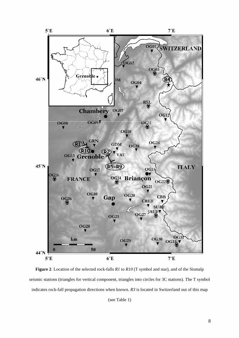
Only events recorded by at least three seismic stations were considered in this study. Figure 2

shows the location of the 10 selected rock-falls and rock-fall avalanches (R1 to R10) and of the 39

Sismalp seismological stations (out of a total of 44) installed north of the 44°N parallel. Two events

(R1, La Palette, and R10, La Dent du Loup) are located 15 km north-west of Grenoble, six (R2,

Versaire, and R5 to R9, Saint-Antoine valley) are clustered 30 to 40 km east of Grenoble, and the

remaining two occurred near the Swiss and Italian borders (R6, Les Drus) or in Switzerland (R3,

Sandalp). Eight rock-falls (R1, R3 and R5 to R10) occurred in limestone, one in amphibolite (R2) and

one in granite (R4). All sites exhibit near vertical slopes (over 70°) in or under the source zone, which

implies a free-fall phase during the movement (Cruden and Varnes, 1996).

The main characteristics of the 10 rock-fall events are listed in Table 1. They were obtained from

international publications (R1, R3, R10) and unpublished geotechnical reports (R2, R4, R5 to R9). Fall

volumes vary over a wide range from 2 103 m3 to 1.75 106 m3, for total drop heights between 270 and

820 m and run out distances between 190 and 1300 m.

The La Palette rock-fall (event R1) occurred in the upper part of a 250 m high, 70° dipping cliff

composed of thick limestone beds dipping 10° to 30° transversely to the slope (Frayssine and Hantz,

2006). The initial failure mechanism is a slide along a 45° dipping joint; the sliding mass (2 104 m3)

fell 170 m down to the underlying 50° to 30° dipping marly slope, where it propagated up to 450 m

from the failure scarp. The Versaire rock-fall (R2) occurred in the upper part of a 150 m high, 70°

dipping cliff, made of massive amphibolite. The initial failure mechanism is a slide; the sliding mass

(5 104 m3) fell 100 m down to the underlying 50° dipping amphibolite slope, where it propagated up to

250 m from the failure scarp. The Sandalp rockfall (R3) took place in the middle part of a 700 m high

rock wall, which consists in thick near-horizontal limestone beds (Keusen, 1998). The rock mass (1.75

106 m3) initially slid on 45° dipping schistosity planes, jumped over a 100 m high, 80° dipping cliff,

moved on a 35° dipping limestone slope and stopped in the valley with a runout distance of 1300 m.

7

Due to the intense schistosity of the rock mass, an important part of the avalanche deposit consists in

fine particles. The Drus rockfall (R4; Ravanel and Deline, 2006) took place in the middle part a 700 m

high, 75° dipping granite wall, in the Mont Blanc Massif. The failure mechanism might have been

topple or slide and the drop height reached 450 m. Between January 1998 and June 1999, five

rockfalls (R5 to R9) affected a 500 m high cliff made of thin folded limestone beds, in the Saint-

Antoine valley. Volumes ranged from 3 104 to 1 105 m3. They occurred at different heights in the

middle part of the cliff which dips 70°. The first two rockfalls (R5 and R6) involved tall columns with

beds dipping opposite to the slope. The failure mechanisms might have been topple or slide, with a fall

height of 90 m to 100 m. The three following ones (R7 to R9) were located higher in the cliff (fall

height of 190 m) and were slides along bedding planes, steeply dipping towards the slope. The fallen

masses then propagated on a slope made of marl and limestone thin layers, whose slope angle

decreases from 65° to 25°. Finally, the Dent du Loup rockfall (R10) occurred in a 200 m high, 70°

dipping cliff, made of thick limestone beds dipping 10° to 30° opposite to the slope (Frayssines and

Hantz, 2006). The initial failure mechanism is a stepped slide on 75° dipping joints. The sliding mass

(2 103 m3) then fell down to the underlying 35° dipping scree slope, where it propagated up to 300 m

from the failure scarp.

All these rock failures took place in a steep cliff (with a slope of at least 70°) and were followed by

a free-fall phase. Considering the volume threshold (104 m3) proposed by Hungr et al. (2001), all these

events should be classified as rock avalanches, except the Dent du Loup rock-fall (R10) whose size (2

103 m3) is too small. However, 8 of the events have a volume between 104 m3 and 105 m3 which is the

other threshold proposed by Evans and Hungr (1993). Thus, the limits between a rock-fall and a rock

avalanche cannot be defined precisely, as the interactions between the blocks progressively increase

with the number of blocks and the volume. Only the Sandalp event (R3) can be unambiguously

classified as rock avalanche. For simplicity’s sake, we will use the general term rock-fall in the

following, except when specifically discussing the mechanisms (fragmental rock-fall or rock-fall

avalanche).

8

Figure 2. Location of the selected rock-falls R1 to R10 (T symbol and star), and of the Sismalp

seismic stations (triangles for vertical component, triangles into circles for 3C stations). The T symbol

indicates rock-fall propagation directions when known. R3 is located in Switzerland out of this map

(see Table 1)

9

LOCATION DATE (GMT) Longitude

(E) Latitude

(N)

Ns EVENT V (m3) Hf (m)

Dp (m)

H t (m)

Ep (GJ) ML Mrf

Es

(MJ) Es/Ep

20/04/1992 07:07:14

5°58 45°24 4 R1 20000 170 450 450 85 1.2 1.5 10.8 1.27E-04

28/03/1995 14:24:18

5°96 45°12 15 R2 50000 100 250 270 125 1.6 1.8 26.2 2.09E-04

03/03/1996 18:30:59

8°65 46°46 7 R3 1750000 150 1300 800 6560 2.8 2.1 84.4 1.29E-05

17/09/1997 23:23:20

6°95 45°93 12 R4 14000 450 450 - 158 1.7 1.8 27.4 1.74E-04

22/01/1998 14:58:09

6°01 45°05 9 R5 100000 90 995 780 225 0.9 1.2 4.4 1.93E-05

22/01/1998 15:07:00

6°01 45°05 11 R6 100000 100 880 780 250 1.2 1.5 9.9 3.98E-05

29/06/1998 13/06/35

6°01 45°05 21 R7 65000 190 940 820 309 1.6 1.6 17.8 5.76E-05

30/06/1998 20:42:56

6°01 45°05 10 R8 35000 190 940 820 166 1.3 1.5 9.3 5.60E-05

08/06/1999 22:33:39

6°01 45°05 11 R9 30000 190 190 820 143 1.1 1.4 8.1 5.71E-05

04/01/2001 23:37:47

5°62 45°22 3 R10 2000 130 300 270 6,5 1.2 1.5 11.3 1.74E-03

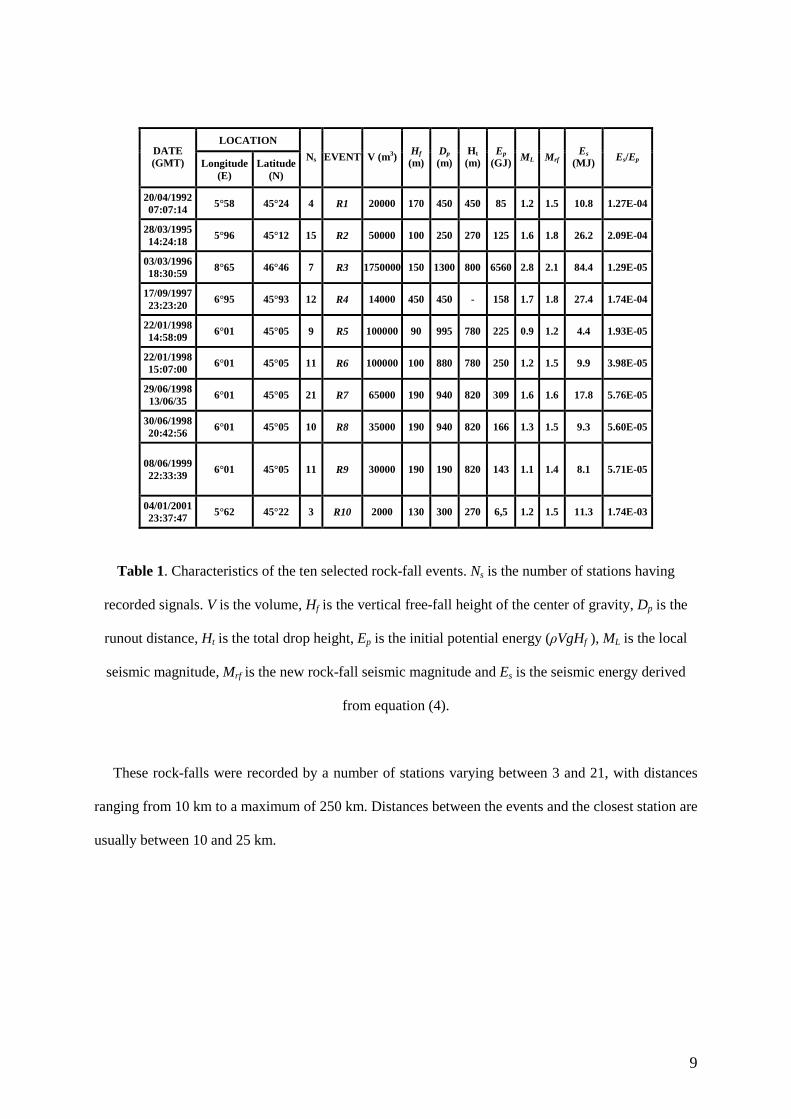
Table 1. Characteristics of the ten selected rock-fall events. Ns is the number of stations having

recorded signals. V is the volume, Hf is the vertical free-fall height of the center of gravity, Dp is the

runout distance, Ht is the total drop height, Ep is the initial potential energy (ρVgHf ), ML is the local

seismic magnitude, Mrf is the new rock-fall seismic magnitude and Es is the seismic energy derived

from equation (4).

These rock-falls were recorded by a number of stations varying between 3 and 21, with distances

ranging from 10 km to a maximum of 250 km. Distances between the events and the closest station are

usually between 10 and 25 km.

10

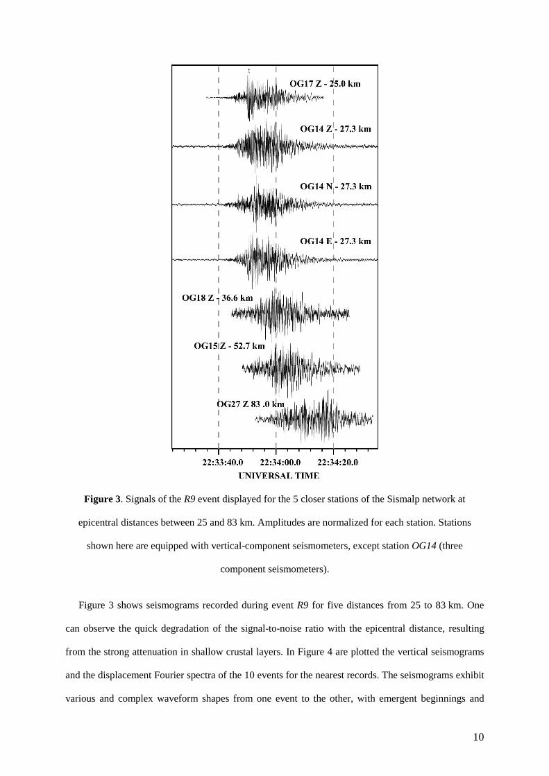
Figure 3. Signals of the R9 event displayed for the 5 closer stations of the Sismalp network at

epicentral distances between 25 and 83 km. Amplitudes are normalized for each station. Stations

shown here are equipped with vertical-component seismometers, except station OG14 (three

component seismometers).

Figure 3 shows seismograms recorded during event R9 for five distances from 25 to 83 km. One

can observe the quick degradation of the signal-to-noise ratio with the epicentral distance, resulting

from the strong attenuation in shallow crustal layers. In Figure 4 are plotted the vertical seismograms

and the displacement Fourier spectra of the 10 events for the nearest records. The seismograms exhibit

various and complex waveform shapes from one event to the other, with emergent beginnings and

11

several late energetic phases that we will attempt to interpret further in this paper. The corner

frequency of the spectra, marked by an arrow in Figure 4, is always close to 1 Hz whatever the event,

showing that 1-Hz velocimeters only record the high-frequency part of ground motion. These results

support the deployment of broad-band seismometers for analyzing the frequency content of rock-fall

signals.

Figure 4. Vertical seismograms and corresponding displacement Fourier spectra measured at the

closest station for the 10 events R1 to R10. The time scale is different for each record. Arrows indicate

corner frequencies.

Table 1 lists location and characteristics for the 10 events. The free-fall drop height (Hf) varies

from 90 to 450 m and the potential energy values (Ep) values are between 6.5 and 6560 GJ for

volumes ranging from 2 103 to 1.75 106 m3. Table 1 also includes local seismic-magnitude values (ML)

provided by the Sismalp network, using the Richter empirical model (1958). These values are between

0.9 and 2.8. Except for event R3 (ML = 2.8), other rock-falls have low magnitudes (0.9-1.7), actually

very close to -and sometimes beyond- the lowest magnitude detectable by the network, estimated to

ML= 1.3 and twice lower than the one assessed for the network deployed in the Yosemite valley

(Myers et al., 2000). Moreover, locating rock-falls with emergent P onsets and unclear S onsets is a

12

challenge difficult to face by a seismic network, although other types of seismic arrays such as

antennas might have better capabilities in this respect. The limited number of observed events (10) and

of the corresponding records (103 in totals) partly results from the relative sparseness of the stations

and from the wave attenuation in the upper crust. However, as pointed out by Weichert et al. (1994)

and suggested by the low ML values in Table 1, the poor efficiency of potential to seismic energy

conversion is probably a significant limiting factor, the effect of which will be addressed further in this

paper.

Seismic record analysis and rock-fall seismic magnitude scale

Our aim is to characterize rock-falls from the analysis of the recorded seismograms. In this part, the

event is treated as an entity (we do not separate the detachment, impact and propagation phases) in

order to have a global characteristic. The first option is to compare rock-falls in terms of seismic

magnitude, in a way similar to what was done for earthquakes. The ML magnitude scale was defined

from the maximum recorded displacement (Richter, 1935 and 1958), for segregating large, moderate

and small shocks. The relation between the maximum seismographic amplitudes for a given shock at

various epicentral distances was empirically built and it was assumed that the ratio of the maximum

amplitudes registered by similar instruments at equal epicentral distances for two given shocks is a

constant. Richter then defined the ML magnitude as the logarithm of the ratio of the amplitude of the

given shock to that of a standard shock at the same epicentral distance. The standard shock (seismic

magnitude equal to 0) was arbitrary defined as an earthquake for which the maximum displacement (in

millimeter) recorded on a standard Wood-Anderson seismometer is equal to one micrometer at

100 km. The so-called Richter attenuation law for distances between 25 and 600 km was published in

1935 by Richter. Kradolfer and Mayer-Rosa (1988) showed that this law satisfactorily fitted the

observed amplitude decay for earthquakes in the Alps, and it is currently used by Sismalp to compute

ML magnitudes (Thouvenot et al., 2003).

For defining a seismic magnitude scale for rock-falls, it is first necessary to determine the relation

between the maximum seismographic amplitudes of a given rock-fall at various distances. Due to the

13

small number of available events and records (67 vertical-component records), the following simple

attenuation relationship was used (Ambraseys et al, 1996; Gasperini, 2002; Berge-Thierry et al, 2003):

10 10log ( ) log ( )m l rPGD b b M b r σ= + + ± (1)

where PGD is the peak ground displacement, ML the local seismic magnitude, r the epicentral

distance (km) and σ the standard deviation. Parameters b, bm and br are empirical coefficients

determined from the linear regression on the values of peak displacements and epicentral distances. In

this relation, we propose that the ML magnitude is replaced with Mrf, which will be called the rock-fall

seismic magnitude. In order to both determine the attenuation model coefficients of equation (1) and

the seismic magnitude, an iterative scheme was applied. In a first step, rock-fall seismic magnitudes

Mrf are approximated by ML magnitudes and the coefficients b, (bm Mrf) and br are determined by

fitting equation (1) to the data. Using Richter’s original definition of an ML=0 shock, Mrf values have

been computed from the (bm Mrf) terms. Equation (1) is then updated with these new Mrf values. The

iterative process is stopped when the RMS difference between two iterations is stable. The attenuation

relation obtained for rock-falls is given by:

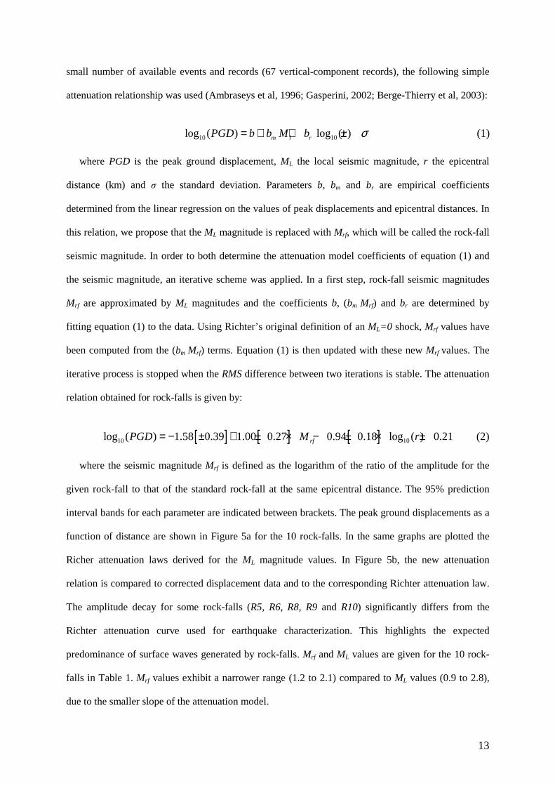
[ ] [ ] [ ]10 10log ( ) 1.58 0.39 1.00 0.27 0.94 0.18 log ( ) 0.21rfPGD M r= − ± + ± × − ± × ± (2)

where the seismic magnitude Mrf is defined as the logarithm of the ratio of the amplitude for the

given rock-fall to that of the standard rock-fall at the same epicentral distance. The 95% prediction

interval bands for each parameter are indicated between brackets. The peak ground displacements as a

function of distance are shown in Figure 5a for the 10 rock-falls. In the same graphs are plotted the

Richer attenuation laws derived for the ML magnitude values. In Figure 5b, the new attenuation

relation is compared to corrected displacement data and to the corresponding Richter attenuation law.

The amplitude decay for some rock-falls (R5, R6, R8, R9 and R10) significantly differs from the

Richter attenuation curve used for earthquake characterization. This highlights the expected

predominance of surface waves generated by rock-falls. Mrf and ML values are given for the 10 rock-

falls in Table 1. Mrf values exhibit a narrower range (1.2 to 2.1) compared to ML values (0.9 to 2.8),

due to the smaller slope of the attenuation model.

14

Figure 5. (a) Comparison between vertical displacement amplitude-distance graphs for the ten rock-

falls, the Richter attenuation model (dashed line) and the new attenuation relation proposed for rock-

falls (solid line) (b) Vertical displacement values as a function of epicentral distances, for the 10 rock-

falls. Displacement values are corrected by the seismic magnitude using equation (2) and compared to

the Richter attenuation model (dashed line) and to the new median model (solid line) plotted with one

standard deviation bounds (dot-dashed lines).

As the corner frequency of the displacement spectra has been shown to be an unreliable source

parameter (Figure 4), due to the frequency cut-off of the short-period seismometers, we investigate the

possibility of using the signal duration for characterizing and discriminating the rock-falls. The

ground-motion duration was computed for all rock-fall seismograms, following the definition

(Trifunac and Brady, 1975) which is the time interval between the points at which 5% and 95% of the

total energy has been recorded. Figure 6 shows the duration-distance graphs for the 10 events in a bi-

15

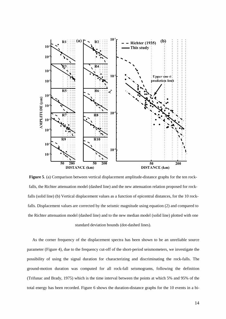
logarithmic diagram, for distances shorter than 100 km. The 40-sec record length on most Sismalp

stations was too small to measure the signal duration for the high-volume event (R3). For events R10,

only three stations exhibit a good signal-to-noise ratio. Data for the remaining 8 events show a regular

increase of the duration with the epicentral distance, resulting from the propagation of waves at

different velocities and from diffusion in the crust. A theoretical relation (equation (3)) was fitted to

each data set and the regression parameters a1 and a2 are given in Table 2, with their 95% prediction

interval bands.

10 1 2 10log ( ( )) log ( )t r a a r= + (3)

EVENT a1 95% 95% 95% 95% P.I. a2 95% 95% 95% 95% P.I. t30 (s)

R1 -0.09 ±3.1 0.85 ±1.01 16.6

R2 1.60 ±0.68 0.37 ±0.18 17.7

R4 2.09 ±1.71 0.29 ±0.5 21.3

R5 2.07 ±3.13 0.35 ±1.08 26.2

R6 1.55 ±3.13 0.42 ±0.12 19.6

R7 2.74 ±0.46 0.1 ±0.32 22.1

R8 1.7 ±1.12 0.35 ±0.34 18.0

R9 1.41 ±1.00 0.41 ±0.26 16.7

All events 1.82 ±0.35 0.33 ±0.09 19.4

Table 2: Regression parameters a1 and a2 of equation (3), with their corresponding 95% prediction

interval , computed for the 8 valuable rock-falls (see text for details), and corresponding t30 values.

The slope parameter a2 varies between 0.1 and 0.85. The a2 values with reasonable prediction

interval bands are between 0.35 and 0.42. A value of 0.33 was found considering all events. As most

signals were recorded in the 20- to 40-km distance range, each rock-fall was characterized by the

ground-motion duration t30 computed at an epicentral distance of 30 km using equation (3). This value,

which is calculated with the global total energy recorded on seismogram, includes all the phases of

rock-falls: detachment, impact and propagation of the mass. Values of t30 given in Table 2 will be

discussed in the next section.

16

Figure 6. Record duration as a function of the epicentral distance r for rock-falls recorded by at least 4

stations.

Comparison between seismic and rock-fall characteristics

Despite the few recorded rock-falls, we attempt to link the measured ground motion characteristics

(rock-fall seismic magnitude, seismic energy and duration) to the rock-fall parameters (fall height Hf,

runout Dp, volume V, and potential energy Ep).

Seismic energy for landslides is hard to assess from seismic records, as it depends on the radiation

pattern which is generally unknown. This difficulty and the scarcity of records explain why previous

works on energy calculation used the formulas established for earthquakes. Wiechert et al. (1994)

considered Richter’s formulas for deriving the seismic energy released by several landslides from MS

and M L. In this study, we applied Kanamori’s (1977) equation.

10log 1.5 4.8s sE M= + (4)

where Es is in joules and Ms is the surface wave magnitude. Ms was replaced by Mrf for computing

Es values for the 10 rock-falls given in Table 1. This relation is very close to the one proposed by

Richter (1958) from surface waves.

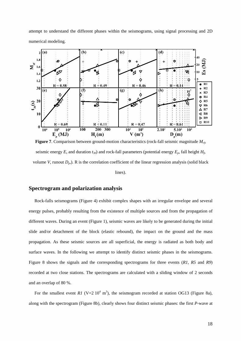
Figure 7 compares in a systematic way the 3 ground-motion and the 4 rock-fall characteristics. As

Es and Mrf are linked, they are plotted in the same graphs with different ordinate values. The

comparison of the seismic energy Es with the potential energy Ep (Figure 7a) shows that only a very

17

small amount of the fall energy is transmitted as seismic waves. The Es/Ep ratio varies between 10-6

and 10-3 (see Table 1). These results agree with the energy conversion values (also between 10-6 and

10-3) found by Weichert et al. (1994) from MS values for rockslides. They highlight the strong

influence of nonlinear effects during the impact. In particular, the highly variable geotechnical site

conditions of the impact zone (from soil to rock) probably explain the large variation of Es/Ep ratios

and the poor correlation between Mrf (or Es) and the rock-fall characteristics Hf, V and Dp (correlation

coefficient R lower than 0.5, Figure 7b, c, d). All the events where the rocks fell on a marly slope (R1,

R5 to R9) exhibit Mrf values below the regression line, resulting from the low coefficient of restitution

of the slope surface. Two data points (R3 and R5) are systematically far from the best regression line.

R5 is the first rock-fall in a sequence of 5 events that occurred in the same place and shows an

unexpected low magnitude value, compared to the other events. It occurred in winter and the mass

failed on a snow layer which could have absorbed a part of the energy, particularly on such a steep

slope (65°). Event R3 exhibits a relatively high magnitude for the values of fall height and runout (Fig.

7b and 7c). In Figure 7b, the vertical distance to the line could result from the initial sliding phase

which contributed to the seismic energy and was not considered in the height-fall estimation. No

explanation was found for the magnitude-runout graph which shows a very poor correlation. On the

contrary, the signal duration t30 exhibits a better correlation with the potential energy (R= 0.69, Figure

7e), with the runout (R= 0.61, Figure 7h) and to a lesser extent with the volume (R= 0.47, Figure 7g).

No correlation was found between the fall height Hf and the ground-motion duration t30 (Figure 7f).

Although limited in number, these results show that, contrary to earthquakes, the seismic energy

derived from records can not characterize rock-falls. Alternatively, the signal duration t30 is more

promising. The good correlation between t30 and Dp indicates that the signal duration, which conveys

information on the different phases of the failure process, is controlled by the propagation phase of the

rock-fall. As the runout distance increases with the rock-fall volume V (Legros, 2002), correlations are

also found between t30 and the rock-fall characteristics Ep and V. However, the limited number of

events considered in this study does not allow us to propose quantitative relationships between these

parameters, and these preliminary results should be validated in the future for a larger number of

events. Due to the limited success of global seismic parameters for characterizing rock-falls, we

18

attempt to understand the different phases within the seismograms, using signal processing and 2D

numerical modeling.

Figure 7. Comparison between ground-motion characteristics (rock-fall seismic magnitude Mrf,

seismic energy Es and duration t30) and rock-fall parameters (potential energy Ep, fall height Hf,

volume V, runout Dp,). R is the correlation coefficient of the linear regression analysis (solid black

lines).

Spectrogram and polarization analysis

Rock-falls seismograms (Figure 4) exhibit complex shapes with an irregular envelope and several

energy pulses, probably resulting from the existence of multiple sources and from the propagation of

different waves. During an event (Figure 1), seismic waves are likely to be generated during the initial

slide and/or detachment of the block (elastic rebound), the impact on the ground and the mass

propagation. As these seismic sources are all superficial, the energy is radiated as both body and

surface waves. In the following we attempt to identify distinct seismic phases in the seismograms.

Figure 8 shows the signals and the corresponding spectrograms for three events (R1, R5 and R9)

recorded at two close stations. The spectrograms are calculated with a sliding window of 2 seconds

and an overlap of 80 %.

For the smallest event R1 (V=2 104 m3), the seismogram recorded at station OG13 (Figure 8a),

along with the spectrogram (Figure 8b), clearly shows four distinct seismic phases: the first P-wave at

19

3 seconds, a lower-frequency wave (around 2 Hz) arriving about 3 seconds later, a high-frequency

wave (from 3 to 10 Hz) at 9 seconds and a second low-frequency energetic wave (2 Hz) 3 seconds

later, just before the signal slowly begins to decrease. The time difference (6 seconds) between the

first onset and the second high-frequency wave is compared to the theoretical fall duration Df given by

the equation:

2 f

f i d

HD t t

g

×= − = (7)

where ti is the impact time, td is the time of the mass detachment, Hf is the fall height (170 m for

R1) and g is the gravity constant (9.81 m/s²). The computed fall duration (6.2 s for R1, see Table 3 and

solid line in Figure 8) is consistent with the observed time difference, supporting the existence of at

least two seismic sources: one corresponding to the initial rupture associated with an elastic rebound

during the detachment, and the other generated at the rock impact on the slope. In Figure 8a are drawn

two solid vertical lines showing the first onset time td and the impact time ti. The signal associated

with the impact has higher amplitude and higher frequency, compared to the one observed during the

elastic rebound phase (Figure 8b). In the same figure are also shown with vertical dashed lines the

theoretical times tdS and tiS of the surface waves generated during the mass detachment and impact,

estimated from the seismic model used for earthquake location (Paul et al, 2001).

Event Drop

Height (m)

Station Fall

duration Df (s)

Distance (km)

td (s) ti (s) tdS (s)

tiS (s)

OG13 23.9 3.3 9.5 6.2 12.4 R1 190

OG17 6.2

40.2 6.9 13.1 11.8 18,0

OG17 25,0 3.6 7.8 6.6 10.9 R5 90

OG14 4.3

27.3 4.2 8.4 7.5 11.8

OG17 25,0 3.9 10.1 6.9 13.1 R9 190

0G14 6.2

27.3 4.3 10.5 7.6 13.9

Table 3. Arrival times of P and surface waves for the three rock-falls R1, R5 and R9. td : arrival time

of the P-wave due to the block detachment, as measured on the seismograms; ti : theoretical impact

time obtained by adding the fall duration to td.; tdS and tiS are the computed surface wave arrival times

for the detachment and the impact, respectively.

20

Computed times are given in Table 3, along with fall-height values and epicentral distances. The fit

between these theoretical times and the two observed low-frequency wave arrivals is excellent,

supporting the interpretation that the four main seismic phases observed in the seismogram are due to

the generation of P and surface waves during the detachment and the impact of the mass.

Figure 8. Vertical- component signals (top) and corresponding spectrograms (bottom) for the R1 (a to

d), R5 (e to h) and R9 (i to l) events recorded at two different stations. The first solid line shows the P-

wave generated during the initial rupture (td) while the second indicates the theoretical impact time

after the fall (ti) computed with formula 7. Dashed lines show the surface-wave arrival times for the

two sources (tdS and tiS for the first and second source, respectively).

A similar analysis was made on the other 5 couples of seismograms and spectrograms and the four

theoretical times are indicated in the same way in Figures 8c to 8l. These times are usually associated

with energy pulses exhibiting frequency variations consistent with the impact (high frequency) or with

the arrival of surface waves (low frequency). However, the seismograms are globally more complex.

On the one hand, some features can be obscured by the superposition of two seismic phases,

depending on the relation between the fall duration and the difference between the propagation times

of P and surface waves. This is observed for the second record (station OG17, Figure 8c) of event R1,

21

where P-waves generated by the impact interfere with surface waves radiated during the detachment.

On the other hand, the source mechanism for the two other greater rock-falls R5 and R9 is clearly

more complex than the one proposed for R1, as shown by the presence of energy pulses later in the

signal (Figures 8e, 8g, 8i, 8k). In particular, the seismograms and spectrograms for rock-fall R5

(V= 1 105 m3) suggest a multi-fall sequence and/or the generation of waves during the mass

propagation. However, the time shift between the source detachment and the impact is consistent with

the theoretical free-fall duration. As stated before, the late slowly decreasing-amplitude part of the

signal is controlled by the propagation phase, as shown by the relation between the signal duration and

the runout distance.

In order to validate the interpretation of P-waves and surface waves, wave polarization analyses

were carried out on the available 3-component stations. Figures 9 and 10 show the seismograms

recorded at station OG14 and the particle motions for the rock-falls R5 and R9, respectively. The

polarization analysis was performed on short time windows (0.5 to 1.5 seconds, according to the wave

period) at the arrival times (td, ti, tdS and tiS) of the four identified waves. At td and ti times (Figures 9b,

9d, 10b and 10d), the particle motions have the characteristics of a P-wave, mainly vibrating along a

particular direction in the radial vertical plane, with an incidence angle between 45° and 60°. At tdS and

tiS times (Figures 9c, 9e, 10c and 10e), the particle motions clearly exhibit an elliptical polarization

typical of surface waves, with however a difference in the polarization direction. For both rock-falls,

surface waves generated during the detachment (Figures 9c and 10c) are Rayleigh-type waves

polarized in the propagation plane, consistently with the approximation of the elastic rebound by a

vertical force. On the contrary, the surface waves radiated at the time of the impact also include Love-

type waves with a significant tangential component (Figures 9e and 10e), particularly for event R9.

Both rock-falls moved in a direction perpendicular to the line linking the events to the station OG14

(Figure 2). As the slope at the impact area is greater than 50° for the two events, a near vertical impact

then induces a strong parallel-to-the-surface shear force, which generates Love-type surface waves at

station OG14. Additional Love-type waves are also observed in the later part of the signals (not

shown) and could result from the shearing due to the sliding mass if the movement evolves to a rock

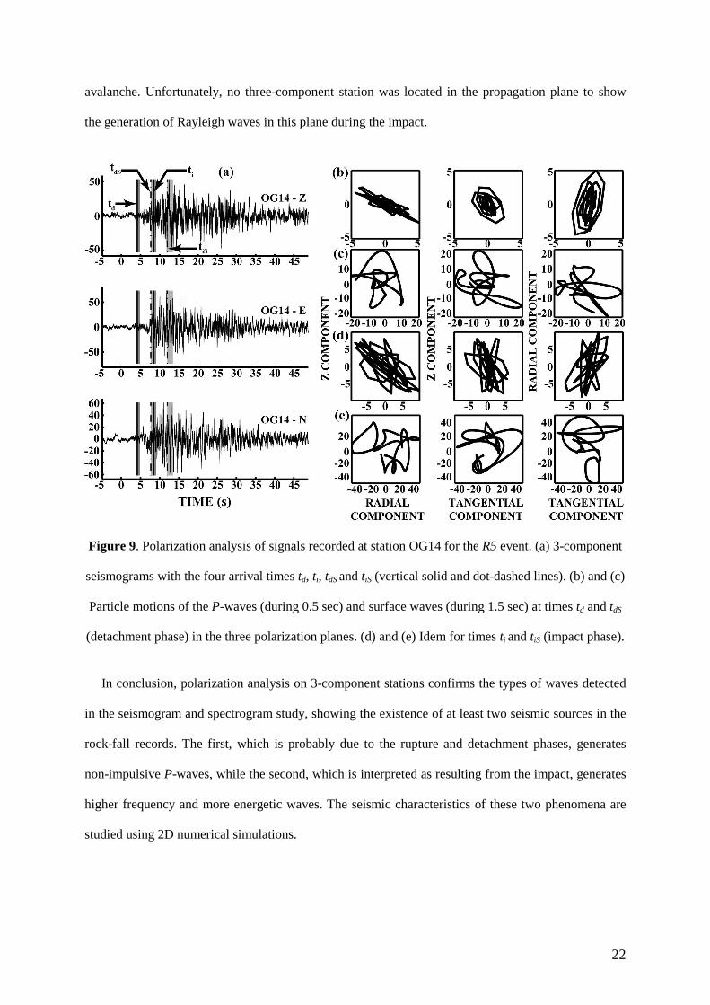
22

avalanche. Unfortunately, no three-component station was located in the propagation plane to show

the generation of Rayleigh waves in this plane during the impact.

Figure 9. Polarization analysis of signals recorded at station OG14 for the R5 event. (a) 3-component

seismograms with the four arrival times td, ti, tdS and tiS (vertical solid and dot-dashed lines). (b) and (c)

Particle motions of the P-waves (during 0.5 sec) and surface waves (during 1.5 sec) at times td and tdS

(detachment phase) in the three polarization planes. (d) and (e) Idem for times ti and tiS (impact phase).

In conclusion, polarization analysis on 3-component stations confirms the types of waves detected

in the seismogram and spectrogram study, showing the existence of at least two seismic sources in the

rock-fall records. The first, which is probably due to the rupture and detachment phases, generates

non-impulsive P-waves, while the second, which is interpreted as resulting from the impact, generates

higher frequency and more energetic waves. The seismic characteristics of these two phenomena are

studied using 2D numerical simulations.

23

Figure 10. Polarization analysis of the signals recorded at station OG14 for the R9 event. Same

caption as in Figure 9.

Numerical Modeling

We simulate the fall of a rectangular block detaching from a cliff along a vertical plane (Figure

11a). The size of the block is 40x80m and the fall height is 170 m. The explicit 2D dynamic finite-

element code Plast2 (Baillet et al., 2005; Baillet and Sassi, 2006) is used to simulate detachment,

frictional contact, fall and impact. The motion equation is both spatially and temporally discretized by

using the finite-element method and the 2β explicit time integration scheme (Carpenter et al., 1991),

respectively. In order to ensure stability, the explicit scheme satisfies the usual Courant-Friedrichs-

Levy (CFL) condition ( min)ch(t ξ∆ ≤ ) where ∆t is the time step, h is the element size, c is the wave

speed, and ξ is a positive constant ( 5.0,1 ≈< ξξ in most practical purposes). Correct wave

propagation is obtained by using 10 finite elements per wavelength (Mullen and Belytschko, 1982)

with the absorbing boundary conditions proposed by Stacey (1988). Computations were made with

89,000 quadrilateral finite elements with an element size of 5 m.

24

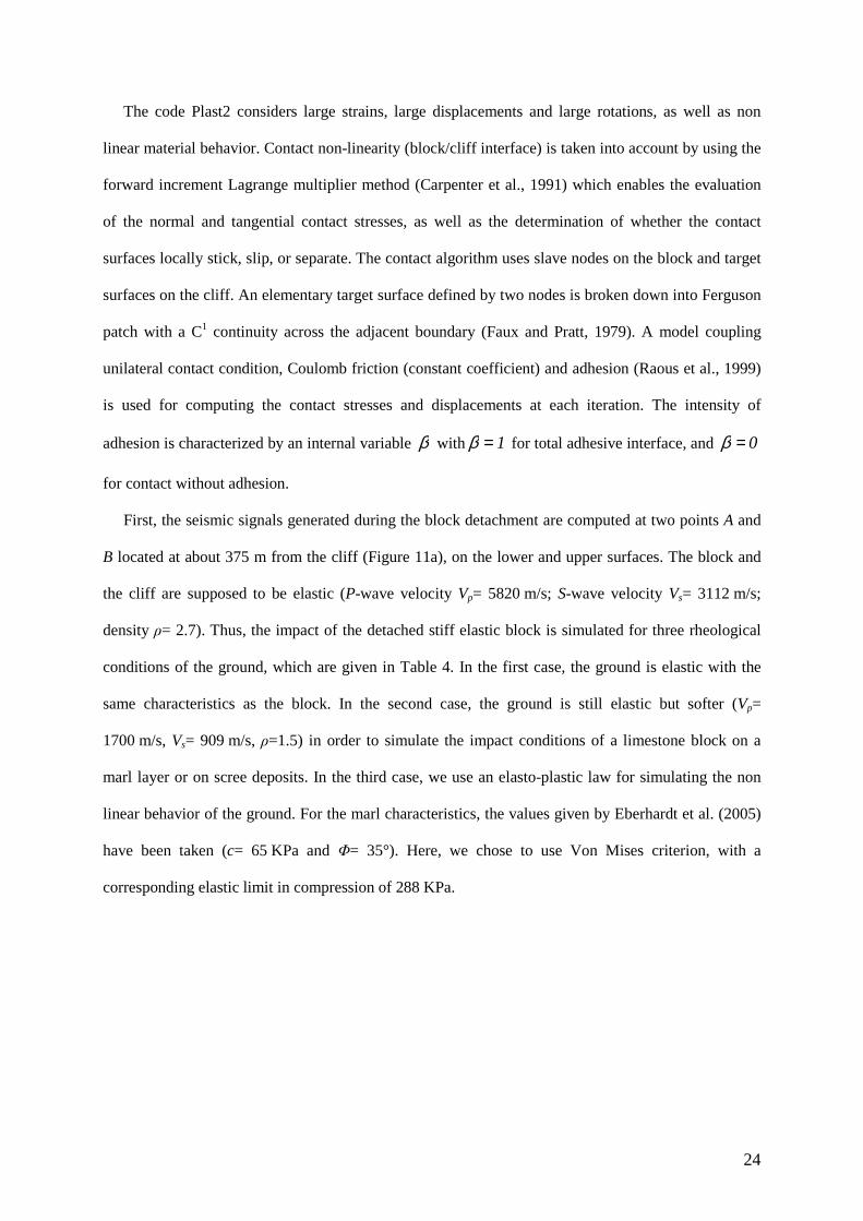
The code Plast2 considers large strains, large displacements and large rotations, as well as non

linear material behavior. Contact non-linearity (block/cliff interface) is taken into account by using the

forward increment Lagrange multiplier method (Carpenter et al., 1991) which enables the evaluation

of the normal and tangential contact stresses, as well as the determination of whether the contact

surfaces locally stick, slip, or separate. The contact algorithm uses slave nodes on the block and target

surfaces on the cliff. An elementary target surface defined by two nodes is broken down into Ferguson

patch with a C1 continuity across the adjacent boundary (Faux and Pratt, 1979). A model coupling

unilateral contact condition, Coulomb friction (constant coefficient) and adhesion (Raous et al., 1999)

is used for computing the contact stresses and displacements at each iteration. The intensity of

adhesion is characterized by an internal variable β with 1=β for total adhesive interface, and 0=β

for contact without adhesion.

First, the seismic signals generated during the block detachment are computed at two points A and

B located at about 375 m from the cliff (Figure 11a), on the lower and upper surfaces. The block and

the cliff are supposed to be elastic (P-wave velocity Vp= 5820 m/s; S-wave velocity Vs= 3112 m/s;

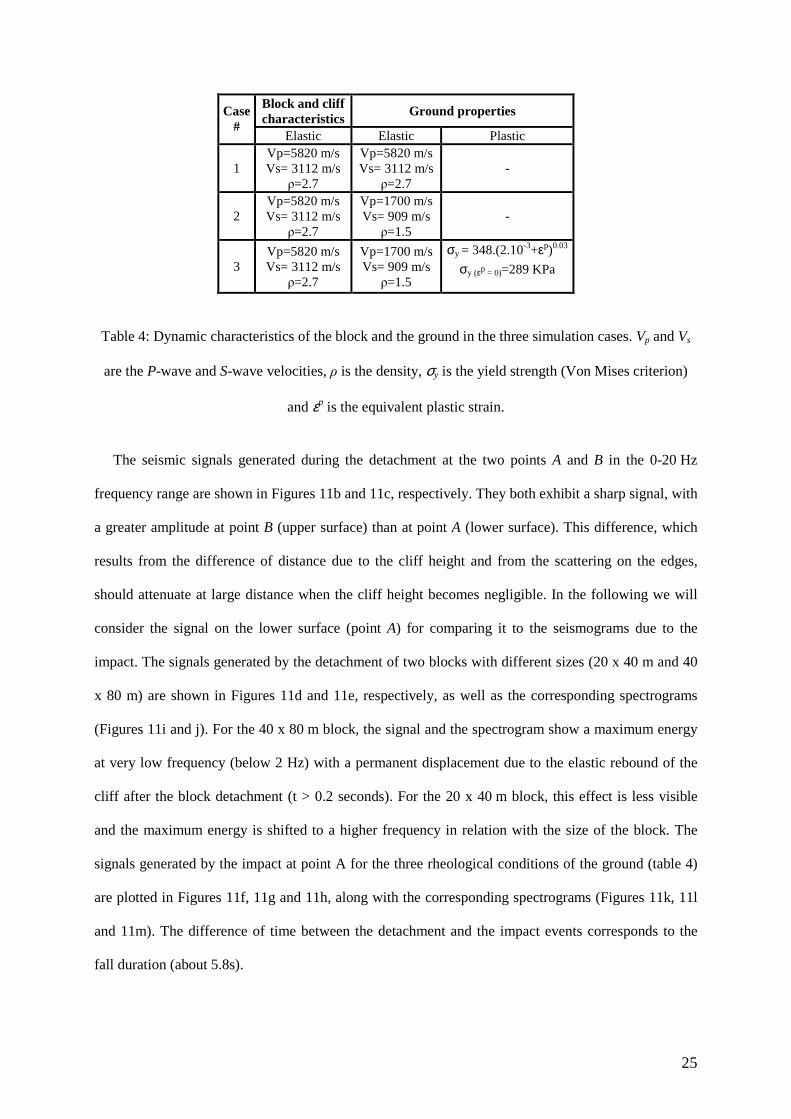
density ρ= 2.7). Thus, the impact of the detached stiff elastic block is simulated for three rheological

conditions of the ground, which are given in Table 4. In the first case, the ground is elastic with the

same characteristics as the block. In the second case, the ground is still elastic but softer (Vp=

1700 m/s, Vs= 909 m/s, ρ=1.5) in order to simulate the impact conditions of a limestone block on a

marl layer or on scree deposits. In the third case, we use an elasto-plastic law for simulating the non

linear behavior of the ground. For the marl characteristics, the values given by Eberhardt et al. (2005)

have been taken (c= 65 KPa and Φ= 35°). Here, we chose to use Von Mises criterion, with a

corresponding elastic limit in compression of 288 KPa.

25

Block and cliff characteristics

Ground properties Case #

Elastic Elastic Plastic

1 Vp=5820 m/s Vs= 3112 m/s

ρ=2.7

Vp=5820 m/s Vs= 3112 m/s

ρ=2.7 -

2 Vp=5820 m/s Vs= 3112 m/s

ρ=2.7

Vp=1700 m/s Vs= 909 m/s ρ=1.5

-

3 Vp=5820 m/s Vs= 3112 m/s

ρ=2.7

Vp=1700 m/s Vs= 909 m/s ρ=1.5

σy = 348.(2.10-3+εp)0.03

σy (εp = 0)=289 KPa

Table 4: Dynamic characteristics of the block and the ground in the three simulation cases. Vp and Vs

are the P-wave and S-wave velocities, ρ is the density, σy is the yield strength (Von Mises criterion)

and εp is the equivalent plastic strain.

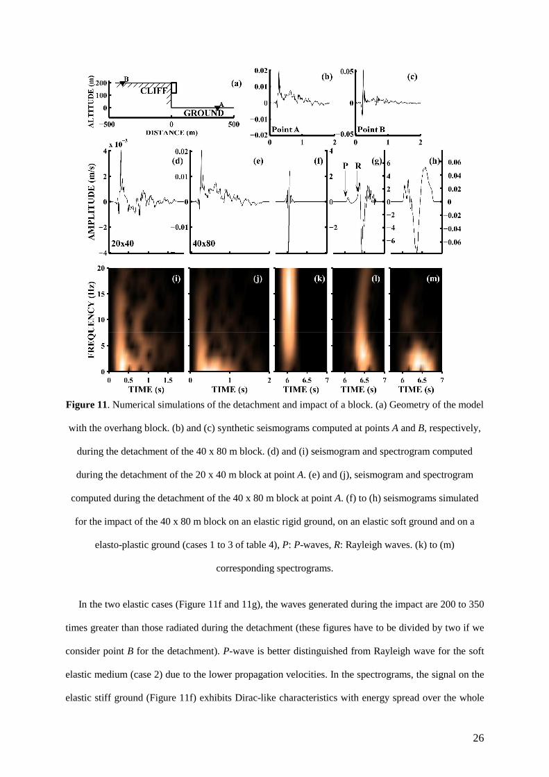
The seismic signals generated during the detachment at the two points A and B in the 0-20 Hz

frequency range are shown in Figures 11b and 11c, respectively. They both exhibit a sharp signal, with

a greater amplitude at point B (upper surface) than at point A (lower surface). This difference, which

results from the difference of distance due to the cliff height and from the scattering on the edges,

should attenuate at large distance when the cliff height becomes negligible. In the following we will

consider the signal on the lower surface (point A) for comparing it to the seismograms due to the

impact. The signals generated by the detachment of two blocks with different sizes (20 x 40 m and 40

x 80 m) are shown in Figures 11d and 11e, respectively, as well as the corresponding spectrograms

(Figures 11i and j). For the 40 x 80 m block, the signal and the spectrogram show a maximum energy

at very low frequency (below 2 Hz) with a permanent displacement due to the elastic rebound of the

cliff after the block detachment (t > 0.2 seconds). For the 20 x 40 m block, this effect is less visible

and the maximum energy is shifted to a higher frequency in relation with the size of the block. The

signals generated by the impact at point A for the three rheological conditions of the ground (table 4)

are plotted in Figures 11f, 11g and 11h, along with the corresponding spectrograms (Figures 11k, 11l

and 11m). The difference of time between the detachment and the impact events corresponds to the

fall duration (about 5.8s).

26

Figure 11. Numerical simulations of the detachment and impact of a block. (a) Geometry of the model

with the overhang block. (b) and (c) synthetic seismograms computed at points A and B, respectively,

during the detachment of the 40 x 80 m block. (d) and (i) seismogram and spectrogram computed

during the detachment of the 20 x 40 m block at point A. (e) and (j), seismogram and spectrogram

computed during the detachment of the 40 x 80 m block at point A. (f) to (h) seismograms simulated

for the impact of the 40 x 80 m block on an elastic rigid ground, on an elastic soft ground and on a

elasto-plastic ground (cases 1 to 3 of table 4), P: P-waves, R: Rayleigh waves. (k) to (m)

corresponding spectrograms.

In the two elastic cases (Figure 11f and 11g), the waves generated during the impact are 200 to 350

times greater than those radiated during the detachment (these figures have to be divided by two if we

consider point B for the detachment). P-wave is better distinguished from Rayleigh wave for the soft

elastic medium (case 2) due to the lower propagation velocities. In the spectrograms, the signal on the

elastic stiff ground (Figure 11f) exhibits Dirac-like characteristics with energy spread over the whole

27

frequency range (Figure 11k), while in the soft elastic case, the energy is more concentrated between 1

and 10 Hz (Figure 11l). Although the synthetic signals are simulated at small distance from the source,

these results agree with the observations made on the real seismograms, that the signal associated to

the impact has higher amplitude and a higher frequency, compared to the one observed during the

detachment phase. However, the real amplitude difference is not as high as the one simulated and a

ground plastic behavior is tested in order to evaluate the nonlinear effect on the wave characteristics

(Figures 11h and 11m).

The introduction of plasticity in the ground with soft elastic characteristics dramatically decreases

the impact amplitude by a factor 100 and strongly affects the spectral energy which concentrates

below 5 Hz. The signal generated during the impact still exhibits greater amplitude (2 to 3.5) than the

one due to the detachment, with a lower ratio range. This ratio is comparable to the one observed on

measured seismograms (compare Figures 8 and 11). Even with a simple plastic law, these numerical

results explain some of the main characteristics of observed seismograms and highlight the strong

influence of ground non-linear behavior on the waves generated during the impact. The consequence

is that frequency content and amplitude of the impact-related part of the signal cannot be used for

extracting information on the fallen block or on the rupture mechanism. That analysis has to be

focused on the early part of the seismograms, linked to the detachment phase, which shows spectral

variations with the block size at low frequency.

Conclusions

We analyzed seismograms recorded during rock-falls in the western Alps by the French permanent

seismological network Sismalp with the aim of getting new information on the rock-fall mechanism.

We used records of ten known events which occurred between 1992 and 2001. The study of the peak

ground motions showed that the regional attenuation relation used for earthquakes is inappropriate for

rock-falls. A new empirical attenuation relation for rock-fall-induced motions was derived from the

data set, allowing a rock-fall seismic magnitude to be attributed to each event. In agreement with

previous works, the comparison between the seismic energy and the potential energy released during

rock-falls showed that only a very small amount (between 10-6 and 10-3) of the fall energy is

28

transmitted as seismic waves. It highlights the effect of nonlinear processes (friction, cracking, plastic

deformation) which probably explain the very poor correlation found between the seismic magnitude

Mrf (or Es) and the rock-fall characteristics Hf, V and Dp. These results imply that, contrary to

earthquakes, the peak ground amplitude, dominated by the impact source, is not a good parameter for

characterizing rock-falls. On the other hand, we showed that the signal duration was correlated to the

runout distance, thus confirming the role played by the propagation phase on this characteristic of the

seismogram. As the Sismalp network is equipped with short-period seismometers, it can only be

concluded that the corner frequency f0 is close to or below 1 Hz for the investigated rock-falls.

Another step forward for a more detailed study of the rock-fall dynamic mechanism would be to

remove the propagation effects from the seismic records, using blind deconvolution methods (Liao and

Huang, 2005, Sèbe et al, 2005).

Signal and particle-motion analyses pointed out the complexity of the seismograms, with the arrival

of at least two P-wave trains and two surface-wave trains. We linked these seismic phases to two

distinct sources: the rupture and detachment of the block from the cliff generating an elastic rebound

on the one hand, and the waves radiated during the impact following the fall on the other hand. The

fall phenomenon might include other complex processes (fragmentation of the falling mass,

interaction with the topography during the fall). However, preliminary 2D elastic and plastic

numerical results retrieved the major spectral and amplitude characteristics of the rock-fall records. In

particular, they highlighted the major effect of the plastic deformation on waves generated during the

impact. Our numerical results also showed an influence of the block volume on the low-frequency

content of the waves, suggesting that the first P-wave train could be used for characterizing rock-falls

if high-quality broad-band seismometer records were available.

Acknowledgements We thank S. G. Evans and an anonymous reviewer who provided helpful comments that

improved the manuscript.

29

References Ambraseys, N.N., K.A. Simpson and J.J. Bommer (1996). Prediction of horizontal response spectra in

Europe. Earthq. Eng. Struct. Dyn. 25, 371-400.

Baillet, L., V. Linck, S. D'Errico, B. Laulagnet and Y. Berthier (2005). Finite element simulation of

dynamic instabilities in frictional sliding contact. Journal of Tribology-Transactions of the

Asme 127, 652-657.

Baillet L. and T. Sassi (2006). Mixed finite element methods for the Signorini problem with friction.

Numerical Methods for Partial Differential Equations 22, Issue 6, 1489-1508.

Berge-Thierry, C., F. Cotton, O. Scotti, D.A. Griot-Pommera and Y. Fukushima (2003). New

empirical response spectral attenuation laws for moderate European earthquakes. Journal of

Earthquake Engineering 7, 193-222.

Berrocal, J., A.F. Espinosa and J. Galdos (1978). Seismological and Geological Aspects of Mantaro

Landslide in Peru. Nature 275, 533-536.

Brodsky, E.E., E. Gordeev and H. Kanamori (2003). Landslide basal friction as measured by seismic

waves. Geophysical Research Letters 30, 2236.

Carpenter N.J., R.L. Taylor and M.G. Katona (1991). Lagrange constraints for transient finite element

surface contact. International Journal for Numerical Methods in Engineering 32, 130-128.

Corominas, J. (1996). The angle of reach as a mobility index for small and large landslide. Canadian

Geotechnical Journal 33, 260-271.

Cruden, D.M. and D.J. Varnes (1996). Landslide types and processes. In: Turner, A.K., Schuster, R.L.

(Eds), Landslides : Investigation and Mitigation. Transportation Research Board, National

Academy Press Washington, Special Report 247, DC, 36-75.

Dahlen, F.A. (1993). Single-force representation of shallow landslide sources. Bull. Seism. Soc. Am.

83 , 130-143.

Eberhardt, E., K. Thuro and M. Luginbuehl (2005). Slope instability mechanism in dipping

interbedded conglomerates and weathered marns-the 1999 Rufi landslide, Switzerland.

Engineering Geology 77, 35-56

30

Eissler, H.K. and H. Kanamori (1987). A Single Force Model for the 1975 Kalapana, Hawaii,

Earthquake. Journal of Geophysical Research 92 , 4827-4836.

Evans, S.G. and O. Hungr (1993). The assessment of rockfall hazard at the base of talus slopes:

Canadian Geotechnical Journal, 30, p. 620–636.

Faux, I.D. and M.J. Pratt (1979).Computational geometry for design and manufacture. Mathematics

and application, Elli Horwood Publishers, 360p

Frayssines, M. and D. Hantz (2006) Failure mechanisms and triggering factors in calcareous cliffs of

the Subalpine Ranges (French Alps). Engineering Geology 86, 256-270.

Gasperini, P. (2002), Local magnitude revaluation for recent Italian earthquakes (1981–1996). Journal

of Seismology, 6, 503–524.

Giani, G.P. (1992), Rock slope stability analysis. Balkema, Rotterdam, 362p.

Hasegawa, H.S. and H. Kanamori (1987). Source Mechanism of the Magnitude-7.2 Grand-Banks

Earthquake of November 1929 - Double Couple or Submarine Landslide. Bull. Seism. Soc. Am.

77(6), 1984-2004.

Hsü, K.J. (1975) Catastrophic debris streams (sturzstroms) generated. by rockfalls. Geol Soc Am Bull

86: 129–140.

Hungr, O., S.G. Evans., M.J. Bovis and J.N. Hutchinson (2001). A review of the classification of

landslides of the flow type, Environmental & Engineering Geoscience, 7, 221-238.

Kanamori, H. (1977). The energy release in great earthquake. Journal of Geophysical Research 82,

2981-2987.

Kanamori, H. and J.W. Given (1982). Analysis of Long-Period Seismic-Waves Excited by the May

18, (1980), Eruption of Mount St Helens - a Terrestrial Monopole. Journal of Geophysical

Research 87, 5422-5432.

Kanamori, H., J.W. Given and T. Lay (1984). Analysis of Seismic Body Waves Excited by the Mount

St-Helens Eruption of May 18, 1980. Journal of Geophysical Research 89, 1856-1866.

Keusen H. R., (1998). Die Bergstürze auf der Sandalp 1996 Risikobeurteilung und

Gefahrenmanagement, Bull. Angew. Geol., 3, 89-102.

31

Kradolfer, U. and D. Mayer-Rosa (1988). Attenuation of seismic waves in Switzerland. In:

Recent Seismological Investigations in Europe, Proc. 19th Gen. Ass. Europ. Seism.

Comm., Nauka, Moscow, 481–488.

La Rocca, M., D. Galluzzo, G. Saccorotti, S. Tinti, G.B Cimini. and E. Del Pezzo (2004). Seismic

Signals Associated with Landslides and with a Tsunami at Stromboli Volcano, Italy. Bull.

Seism. Soc. Am., 94, 1850-1867.

Legros, F. (2002). The mobility of long-runout landslides. Engineering Geology, 63, 301-331.

Liao, B-Y and H-C Huang (2005). Estimation of the Source Time Function Based on Blind

Deconvolution with Gaussian Mixtures. Pure and Applied geophysics 162, 479-494

McSaveney, M.J. (2002). Recent rock-falls and rock avalanches in Mount Cook National Park, New

Zealand. p. 35-70 In: Evans SG, DeGraff JV eds. Catastrophic landslides: effects, occurrence

and mechanisms. Geological Society of America Reviews in Engineering Geology 15.

Mills, H.H. (1991). Temporal Variation of Mass-Wasting Activity in Mount St-Helens Crater,

Washington, USA - Indicated by Seismic Activity. Arctic and Alpine Research 23(4), 417-423.

Mullen, R. and T. Belytschko (1982). Dispersion analysis of finite element semi discretizations of the

two dimensional wave equation. Int. J. Num. Methods. Eng. 18, 11-29.

Myers, S, D. Rock and K. Mayeda (2000). Feasibility of Monitoring Rock Fall in Yosemite Valley

Using Seismic Methods, Open file technical report, 17 p.

Nicoletti, P.G. and M. Sorriso-Valvo (1991). Geomorphic controls of the shape and mobility of rock

avalanches. Geological Society of America Bulletin 103, 1365-1373.

Norris, R.D. (1994). Seismicity of rock-falls and avalanches at three cascade range volcanoes:

Implications for seismic detection of hazardous mass movements. Bull. Seism. Soc. Am. 84,

1925-1939.

Okura, Y., H. Kitahara, T. Sammori and A. Kawanami (2000). The effect of rock-fall volume on

runout distance. Engineering Geology, 58, 109-124.

Paul, A., M. Cattaneo, F. Thouvenot, D. Spallarossa, N. Bethoux and J. Fréchet (2001). A three-

dimensional crustal velocity model of the south-western Alps from local earthquake

tomography. Journal of Geophysical Research 106, 19,367-19,390

32

Raous, M., L. Cangemi and M. Cocu (1999). A consistent model coupling adhesion, friction and

unilateral contact. Computer Methods in Applied Mechanics and Engineering 177, n°3-4, 383-

399.

Ravanel, L. and P. Deline (2006). Nouvelles methodes d’étude de l’évolution des parois rocheuses de

haute montagne : application au cas des Drus. Proceedings of the workshop « Géologie et

Risques Naturels : la gestion des risques au Pays du Mont Blanc», November 16, 2006,

Sallanches, 48-53.

Richter, C.F. (1935). An instrumental earthquake magnitude scale. Bull. Seism. Soc. Am. 25, 1-32.

Richter, C.F. (1958). Elementary Seismology. San Francisco 768 pp.

Sèbe, O., P-Y. Bard and J. Guilbert (2005). Single station estimation of seismic source time function

from coda waves: the Kursk disaster. Geophysical Research Letters 32, L14308

Stacey, R. (1988). Improved transparent boundary formulations for the elastic-wave equation. Short

Note. Bull. Seism. Soc. Am. 78, 2089-2097

Thouvenot, F., J. Fréchet, F. Guyoton, R. Guiguet and L. Jenatton (1990). Sismalp: an automatic

phone-interrogated seismic network for the western Alps. Cahiers du Centre Européen de

Géodynamique et de Séismologie 1, 1-10.

Thouvenot, F., J. Fréchet, L. Jenatton and J.-F. Gamond (2003). The Belledonne Border Fault:

identification of an active seismic strike-slip fault in the western Alps. Geophysical Journal

International 155, 174-192.

Thouvenot, F. and J. Fréchet (2006). Seismicity along the northwestern edge of the Adria microplate.

In N. Pinter et al. (eds) The Adria Microplate: GPS Geodesy. Tectonics and Hazards, Nato

Science Series 61, 335-349.

Tilling, R.I., R.Y. Koyanagi and R.T. Holcomb (1975). Rock-fall Seismicity-Correlation with Field

Observations, Makaopuhi Crater, Kilauea Volcano, Hawaii. Journal of Research of the US

Geological Survey 3, 345-361.

Trifunac, M.D. and A.G. Brady (1975). A study of the duration of strong earthquake ground motion.

Bull. Seism. Soc. Am. 65, 581-626.

Uhrhammer, R. (1996). Yosemite rock fall of July 10, 1996, Seismol. Res. Let., 67,47-48.

33

Weichert, D., R.B. Horner and S.G. Evans (1994). Seismic Signatures of Landslides - the 1990 Brenda

Mine Collapse and the 1965 Hope Rockslides. Bull. Seism. Soc. Am. 84, 1523-1532.

Wieczorek, G., J. Snyder, J. Waitt, M. Morrissey, M. Uhrhammer, R. Harp, E. Norris, R. Bursik,

M. Finewood (2000). The unusual air blast and dense sandy cloud triggered by the July 10,

1996 rock fall at Happy Isles, Yosemite National Park, California, Geol. Soc. Am. Bull., 112,

75-85.

Affiliation and address of authors

Laboratoire de Géophysique Interne et Tectonophysique (LGIT-CNRS)

Université Joseph Fourier

Maison des Géosciences, BP 53

38041 Grenoble Cedex 9

France