analysis of federal agency facility energy reduction potential and
TRANSCRIPT

PNNL-23063
Prepared for the U.S. Department of Energy
under Contract DE-AC05-76RL01830
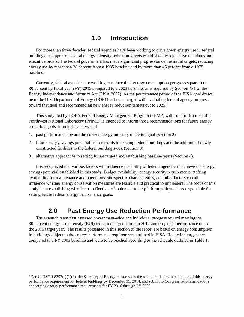
Analysis of Federal Agency Facility Energy Reduction Potential and Goal-Setting Approaches for 2025 KS Judd JA Dirks DM Anderson BE Ford DB Belzer May 2014

Analysis of Federal Agency Facility Energy Reduction Potential and Goal-Setting Approaches for 2025
KS Judd JA Dirks
DM Anderson BE Ford
DB Belzer
May 2014
Prepared for
the U.S. Department of Energy
under Department of Energy Contract DE-AC05-76RL01830
with Battelle Memorial Institute
Pacific Northwest National Laboratory
Richland, Washington 99352

ii
iii
Acronyms and Abbreviations
ARRA American Recovery and Reinvestment Act
Btu British thermal units
BBtu billion British thermal units
CBECS Commercial Building Energy Consumption Survey
CDD cooling degree days
DHS Department of Homeland Security
DOC Department of Commerce
DOD Department of Defense
DOE Department of Energy
DOI Department of the Interior
DOJ Department of Justice
DOL Department of Labor
DOT Department of Transportation
ECM energy conservation measure
EISA Energy Independence and Security Act
EPA Environmental Protection Agency
EUI energy use intensity
FEDS Facility Energy Decision System
FEMP Federal Energy Management Program
FY fiscal year
GSA General Services Administration
GSF gross square footage
HDD heating degree days
HHS Department of Health and Human Services
HUD Department of Housing and Urban Development
HVAC heating, ventilating and air conditioning
LCC life-cycle cost
LPG liquefied petroleum gas
NARA National Archives and Records Administration
NASA National Aeronautics and Space Administration
OMB Office of Management and Budget
OPM Office of Personnel Management
PNNL Pacific Northwest National Laboratory
SF square foot
SI Smithsonian Institution
SIR savings-to-investment ratio
iv
SSA Social Security Administration
State Department of State
TMY typical meteorological year
TRSY Department of the Treasury
TVA Tennessee Valley Authority
USACE Army Corps of Engineers
USDA Department of Agriculture
USPS United States Postal Service
VA Department of Veterans Affairs

v
Contents
1.0 Introduction ................................................................................................................................ 1
2.0 Past Energy Use Reduction Performance ................................................................................... 1
2.1 Government-wide performance .......................................................................................... 2
2.1.1 Federal progress toward EUI reduction goal with projection out to 2015 .............. 2
2.1.2 Observations on Government-wide Trends ............................................................. 4
2.1.3 Changes in Energy Use by Fuel Type ..................................................................... 6
2.2 Agency-specific performance............................................................................................. 8
2.2.1 Department of Defense .......................................................................................... 10
2.2.2 Department of Energy ........................................................................................... 11
2.2.3 Department of Health and Human Services .......................................................... 13
2.2.4 Department of Justice ............................................................................................ 15
2.2.5 Department of Veterans Affairs ............................................................................ 17
2.2.6 General Services Administration ........................................................................... 19
2.2.7 United States Postal Service .................................................................................. 21
3.0 Future Energy Savings Potential in Federal Buildings ............................................................. 23
3.1 Existing Building Retrofits ............................................................................................... 23
3.1.1 Modeling Prototype Federal Buildings ................................................................. 23
3.1.2 EUIs for Prototype Buildings ................................................................................ 25
3.1.3 Estimated Energy Savings Potential from Energy Conservation and Efficiency .. 26
3.1.4 Estimated Renewable Energy Production Potential .............................................. 27
3.1.5 Estimated Cost of Implementation ........................................................................ 28
3.2 Construction of New Buildings ........................................................................................ 30
3.2.1 Newly Constructed Floor Space ............................................................................ 31
3.2.2 Impact of ASHRAE Standards and Other Factors on Newly Constructed
Building EUIs ........................................................................................................ 32
3.2.3 Impact on 2025 EUI of Federal Building Stock .................................................... 34
3.3 Combined Impact of Retrofits and New Construction on Federal Building Stock EUI .. 35
4.0 Alternative Energy Performance Evaluation Approaches ........................................................ 36
4.1 Site vs. Source EUI .......................................................................................................... 37
4.1.1 Description of Source Energy Calculations .......................................................... 37
4.1.2 Benefits and Drawbacks ........................................................................................ 38
4.1.3 Impact on Past Performance .................................................................................. 41
4.1.4 Impact on Future Energy Savings ......................................................................... 41
4.2 Goal-Subject vs. All Buildings ......................................................................................... 43
4.3 FY 2003 vs. Alternative Baseline Years .......................................................................... 45
4.3.1 Weather ................................................................................................................. 45
4.3.2 Other Factors ......................................................................................................... 47

vi
4.4 Single vs. Distinct or Tiered Performance Goals ............................................................. 48
4.5 Intensity vs. Absolute Reduction Goals ........................................................................... 49
4.6 Other Goal-Setting Approaches ....................................................................................... 50
5.0 Conclusions and Recommendations ......................................................................................... 51
6.0 References ................................................................................................................................ 54
Appendix A. Methodology for Estimating Existing Building Retrofits ............................................. 1
Appendix B. Estimating Impact of New Construction on the 2025 Federal Energy Goal: Detailed
Methodology ...........................................................................................................................A-1
Appendix C. Data Sources to Estimate Recent Additions of Federal Floor Space ......................... B-1
Appendix D. Heat Map of Fossil Energy Intensity based on eGRID 2012 .................................... C-1
Figures
1. Energy use, floor space, and energy intensity for the federal government, FY 2003-2012 ............ 3
2. Overall government progress toward facility energy efficiency goals, FY 2003-2012, with
projections to FY 2015 ............................................................................................................... 4
3. Energy use (billion Btus) and floor space (million SF) by agency in FY 2012 .............................. 5
4. Energy use intensity (Btu/SF) of Federal agencies in FY 2012 ...................................................... 5
5. Total energy use (BBtu) by federal agencies in goal-subject buildings, FY 2003-2012 ................ 6
6. Change in energy use by fuel type, FY 2003-2012 ......................................................................... 7
7. Agency contribution to total energy savings by fuel type, FY 2003-2012 ..................................... 9
8. DOD energy use intensity, energy use, and floor space for FY 2003-2012 ................................. 10
9. Change in DOD energy use by fuel type, FY 2003-2012 ............................................................. 11
10. DOE energy use intensity, energy use, and floor space for FY 2003-2012 ................................ 12
11. Change in DOE energy use by fuel type, FY 2003-2012 ........................................................... 13
12. HHS energy use intensity, energy use, and floor space for FY 2003-2012 ................................ 14
13. Change in HHS energy use by fuel type, FY 2003-2012 ............................................................ 15
14. DOJ energy use intensity, energy use, and floor space for FY 2003-2012 ................................. 16
15. Change in DOJ energy use by fuel type, FY 2003-2012 ............................................................ 17
16. VA Energy Use Intensity, Energy Use, and Floor Space for FY 2003-2012 ............................. 18
17. Change in VA energy use by fuel type, FY 2003-2012 .............................................................. 19
18. GSA energy use intensity, energy use, and floor space for FY 2003-2012 ................................ 20
19. Change in GSA energy use by fuel type, FY 2003-2012 ............................................................ 21
20. USPS energy use intensity, energy use, and floor space for FY 2003-2012 ............................... 22
21. Change in USPS energy use by fuel type, FY 2003-2012 .......................................................... 22
22. Proportion of total cost vs. proportion of total energy use by fuel source using the DOE FY
2012 data ................................................................................................................................... 39
23. Percentage of EUI reduction by agency, FY 2008-2012 ............................................................ 41
24. Reduction in site EUI for goal-subject buildings and all buildings, FY 2008-2012 ................... 45
vii
Tables
1. Energy use intensity reduction schedule in EISA ........................................................................... 2
2. Reductions in energy use (BBtu) by fuel type, FY 2003-2012 ....................................................... 7
3. Percent changes in EUI, total energy use, and floor space from FY 2003-2012 ............................ 8
4. Estimated EUI impact of cost-effective energy conservation measures (site energy basis) ........ 26
5. Differences in progress toward current federal reduction targets for DOD and civilian agencies 27
6. Potential 2015-2025 EUI reduction from implementing technically feasible onsite renewable
energy (site energy basis).......................................................................................................... 28
7. Nominal installed costs and associated energy cost savings impacts from efficiency measures
(current dollars) ......................................................................................................................... 29
8. Technology retrofit energy savings opportunities at the end use level (Percent of aggregate
savings) ..................................................................................................................................... 30
9. Floor space and new construction projections, FY 2016-2025 (millions of square feet) ............. 32
10. Impact of new construction meeting ASHRAE Standard 90.1-2010 and a hypothetical future
Standard 90.1-2016 on average building stock EUI in 2025 .................................................... 34
11. Impact of new building construction on 2025 civilian stock EUI............................................... 34
12. Estimated EUI impact from both cost-effective retrofits to existing buildings and federal
energy standards for new construction (site energy basis) ....................................................... 35
13. Fossil-source energy using regional eGRID factors ................................................................... 38
14. Benefits and drawbacks of using site energy versus source energy to calculate EUI reductions39
15. Benefits and drawbacks of using national versus regional source energy factors to calculate
EUI reductions .......................................................................................................................... 40
16. Estimated EUI impact of both cost-effective retrofits to existing buildings and federal energy
standards for new construction (on a source energy basis) ....................................................... 42
17. Illustration of the impact using of site energy vs. source energy on percent of energy savings . 43
18. Benefits and drawbacks of basing energy reduction goals on goal-subject vs. all buildings ...... 44
19. Total heating degree days and cooling degree days for 12 U.S. cities ........................................ 46
20. Possible baseline years and an evaluation of how each year rates against different criteria;
green is a comparatively good year, yellow is neutral, and red is comparatively bad .............. 48
21. Benefits and drawbacks of setting energy intensity vs. absolute reduction goals ....................... 49
22. Estimated EUI impact from both cost-effective retrofits to existing buildings and federal
energy standards for new construction (site energy basis) ....................................................... 52

viii
1
1.0 Introduction
For more than three decades, federal agencies have been working to drive down energy use in federal
buildings in support of several energy intensity reduction targets established by legislative mandates and
executive orders. The federal government has made significant progress since the initial targets, reducing
energy use by more than 28 percent from a 1985 baseline and by more than 46 percent from a 1975
baseline.
Currently, federal agencies are working to reduce their energy consumption per gross square foot
30 percent by fiscal year (FY) 2015 compared to a 2003 baseline, as is required by Section 431 of the
Energy Independence and Security Act (EISA 2007). As the performance period of the EISA goal draws
near, the U.S. Department of Energy (DOE) has been charged with evaluating federal agency progress
toward that goal and recommending new energy reduction targets out to 2025.1
This study, led by DOE’s Federal Energy Management Program (FEMP) with support from Pacific
Northwest National Laboratory (PNNL), is intended to inform those recommendations for future energy
reduction goals. It includes analyses of
1. past performance toward the current energy intensity reduction goal (Section 2)
2. future energy savings potential from retrofits to existing federal buildings and the addition of newly
constructed facilities to the federal building stock (Section 3)
3. alternative approaches to setting future targets and establishing baseline years (Section 4).
It is recognized that various factors will influence the ability of federal agencies to achieve the energy
savings potential established in this study. Budget availability, energy security requirements, staffing
availability for maintenance and operations, site specific characteristics, and other factors can all
influence whether energy conservation measures are feasible and practical to implement. The focus of this
study is on establishing what is cost-effective to implement to help inform policymakers responsible for
setting future federal energy performance goals.
2.0 Past Energy Use Reduction Performance The research team first assessed government-wide and individual progress toward meeting the
30 percent energy use intensity (EUI) reduction targets through 2012 and projected performance out to
the 2015 target year. The results presented in this section of the report are based on energy consumption
in buildings subject to the energy performance requirements outlined in EISA. Reduction targets are
compared to a FY 2003 baseline and were to be reached according to the schedule outlined in Table 1.
1 Per 42 USC § 8253(a)(1)(3), the Secretary of Energy must review the results of the implementation of this energy
performance requirement for federal buildings by December 31, 2014, and submit to Congress recommendations
concerning energy performance requirements for FY 2016 through FY 2025.
2
Table 1. Energy use intensity reduction schedule in EISA
Fiscal Year Reduction Target
2006 2%
2007 4%
2008 9%
2009 12%
2010 15%
2011 18%
2012 21%
2013 24%
2014 27%
2015 30%
Data to support the past-performance analysis came from agency annual energy data reports
submitted to FEMP for the years 2003 through 2012. Because the EUI reduction goal applies only to
“goal-subject” buildings, the results presented below reflect energy savings in those buildings only.
To project compliance with the 30 percent reduction requirement out to 2015, the team estimated
average annual savings over the entire period by agency and applied that annual savings rate to the years
2013-2015. The entire period was used rather than limiting the analysis to recent years in order to control
for recent spikes in energy savings that may have resulted from short-term American Recovery and
Restoration Act (ARRA 2009) investments in building energy efficiency.
2.1 Government-wide performance
2.1.1 Federal progress toward EUI reduction goal with projection out to 2015
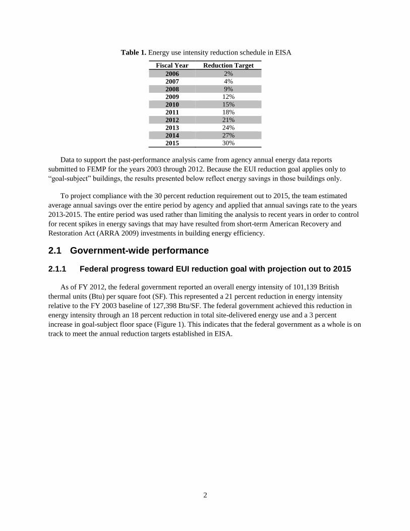
As of FY 2012, the federal government reported an overall energy intensity of 101,139 British
thermal units (Btu) per square foot (SF). This represented a 21 percent reduction in energy intensity
relative to the FY 2003 baseline of 127,398 Btu/SF. The federal government achieved this reduction in
energy intensity through an 18 percent reduction in total site-delivered energy use and a 3 percent
increase in goal-subject floor space (Figure 1). This indicates that the federal government as a whole is on
track to meet the annual reduction targets established in EISA.
3
Figure 1. Energy use, floor space, and energy intensity for the federal government, FY 2003-2012
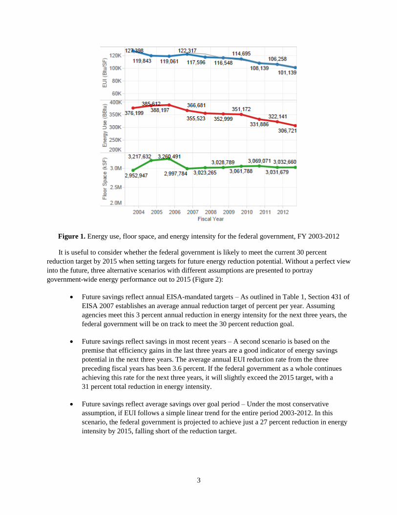
It is useful to consider whether the federal government is likely to meet the current 30 percent
reduction target by 2015 when setting targets for future energy reduction potential. Without a perfect view
into the future, three alternative scenarios with different assumptions are presented to portray
government-wide energy performance out to 2015 (Figure 2):
Future savings reflect annual EISA-mandated targets – As outlined in Table 1, Section 431 of
EISA 2007 establishes an average annual reduction target of percent per year. Assuming
agencies meet this 3 percent annual reduction in energy intensity for the next three years, the
federal government will be on track to meet the 30 percent reduction goal.
Future savings reflect savings in most recent years – A second scenario is based on the
premise that efficiency gains in the last three years are a good indicator of energy savings
potential in the next three years. The average annual EUI reduction rate from the three
preceding fiscal years has been 3.6 percent. If the federal government as a whole continues
achieving this rate for the next three years, it will slightly exceed the 2015 target, with a
31 percent total reduction in energy intensity.
Future savings reflect average savings over goal period – Under the most conservative
assumption, if EUI follows a simple linear trend for the entire period 2003-2012. In this
scenario, the federal government is projected to achieve just a 27 percent reduction in energy
intensity by 2015, falling short of the reduction target.
4
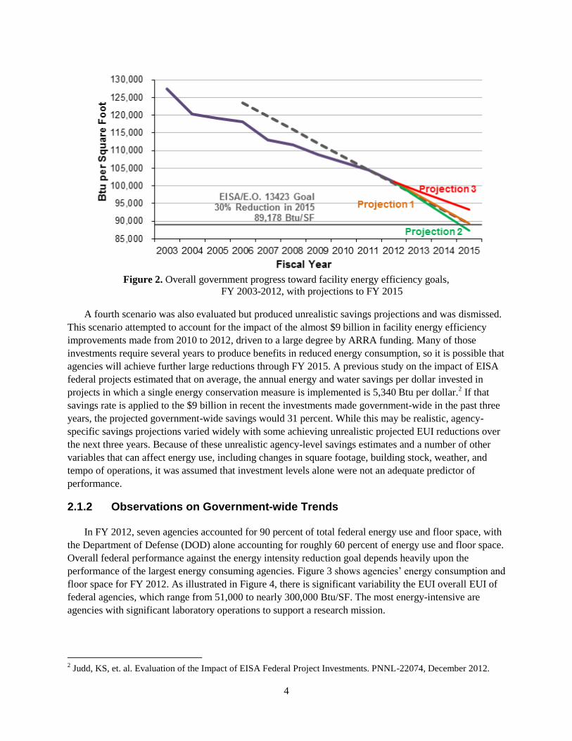
Figure 2. Overall government progress toward facility energy efficiency goals,
FY 2003-2012, with projections to FY 2015
A fourth scenario was also evaluated but produced unrealistic savings projections and was dismissed.
This scenario attempted to account for the impact of the almost $9 billion in facility energy efficiency
improvements made from 2010 to 2012, driven to a large degree by ARRA funding. Many of those
investments require several years to produce benefits in reduced energy consumption, so it is possible that
agencies will achieve further large reductions through FY 2015. A previous study on the impact of EISA
federal projects estimated that on average, the annual energy and water savings per dollar invested in
projects in which a single energy conservation measure is implemented is 5,340 Btu per dollar.2 If that
savings rate is applied to the $9 billion in recent the investments made government-wide in the past three
years, the projected government-wide savings would 31 percent. While this may be realistic, agency-
specific savings projections varied widely with some achieving unrealistic projected EUI reductions over
the next three years. Because of these unrealistic agency-level savings estimates and a number of other
variables that can affect energy use, including changes in square footage, building stock, weather, and
tempo of operations, it was assumed that investment levels alone were not an adequate predictor of
performance.
2.1.2 Observations on Government-wide Trends
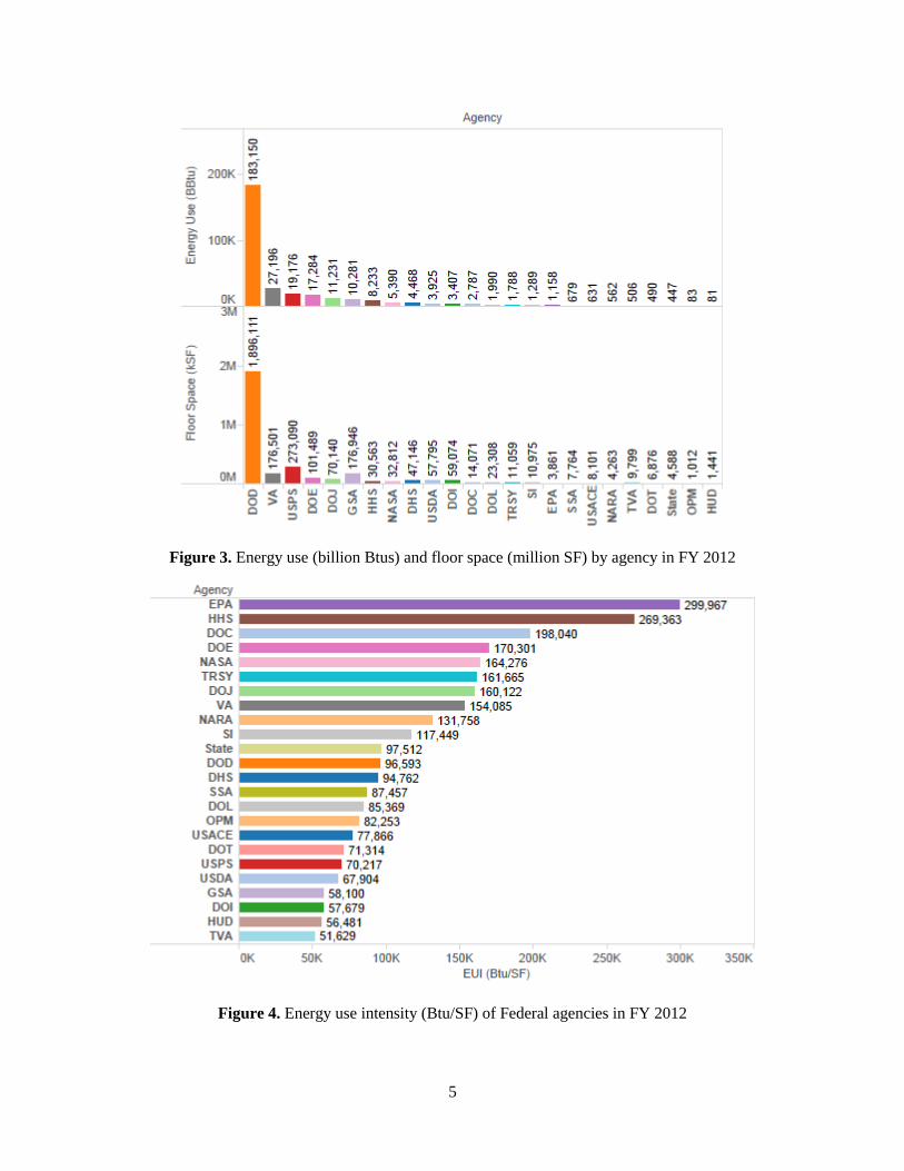
In FY 2012, seven agencies accounted for 90 percent of total federal energy use and floor space, with
the Department of Defense (DOD) alone accounting for roughly 60 percent of energy use and floor space.
Overall federal performance against the energy intensity reduction goal depends heavily upon the
performance of the largest energy consuming agencies. Figure 3 shows agencies’ energy consumption and
floor space for FY 2012. As illustrated in Figure 4, there is significant variability the EUI overall EUI of
federal agencies, which range from 51,000 to nearly 300,000 Btu/SF. The most energy-intensive are
agencies with significant laboratory operations to support a research mission.
2 Judd, KS, et. al. Evaluation of the Impact of EISA Federal Project Investments. PNNL-22074, December 2012.
5
Figure 3. Energy use (billion Btus) and floor space (million SF) by agency in FY 2012
Figure 4. Energy use intensity (Btu/SF) of Federal agencies in FY 2012
6
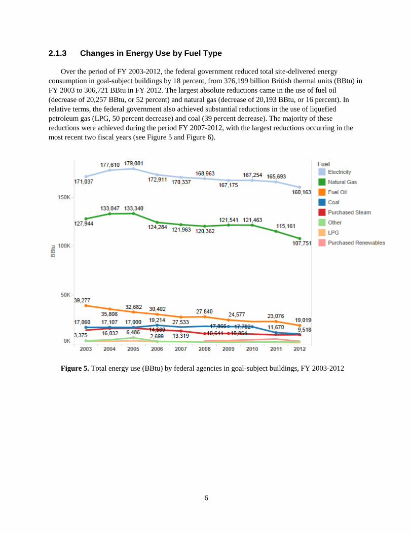
2.1.3 Changes in Energy Use by Fuel Type
Over the period of FY 2003-2012, the federal government reduced total site-delivered energy
consumption in goal-subject buildings by 18 percent, from 376,199 billion British thermal units (BBtu) in
FY 2003 to 306,721 BBtu in FY 2012. The largest absolute reductions came in the use of fuel oil
(decrease of 20,257 BBtu, or 52 percent) and natural gas (decrease of 20,193 BBtu, or 16 percent). In
relative terms, the federal government also achieved substantial reductions in the use of liquefied
petroleum gas (LPG, 50 percent decrease) and coal (39 percent decrease). The majority of these
reductions were achieved during the period FY 2007-2012, with the largest reductions occurring in the
most recent two fiscal years (see Figure 5 and Figure 6).
Figure 5. Total energy use (BBtu) by federal agencies in goal-subject buildings, FY 2003-2012
7
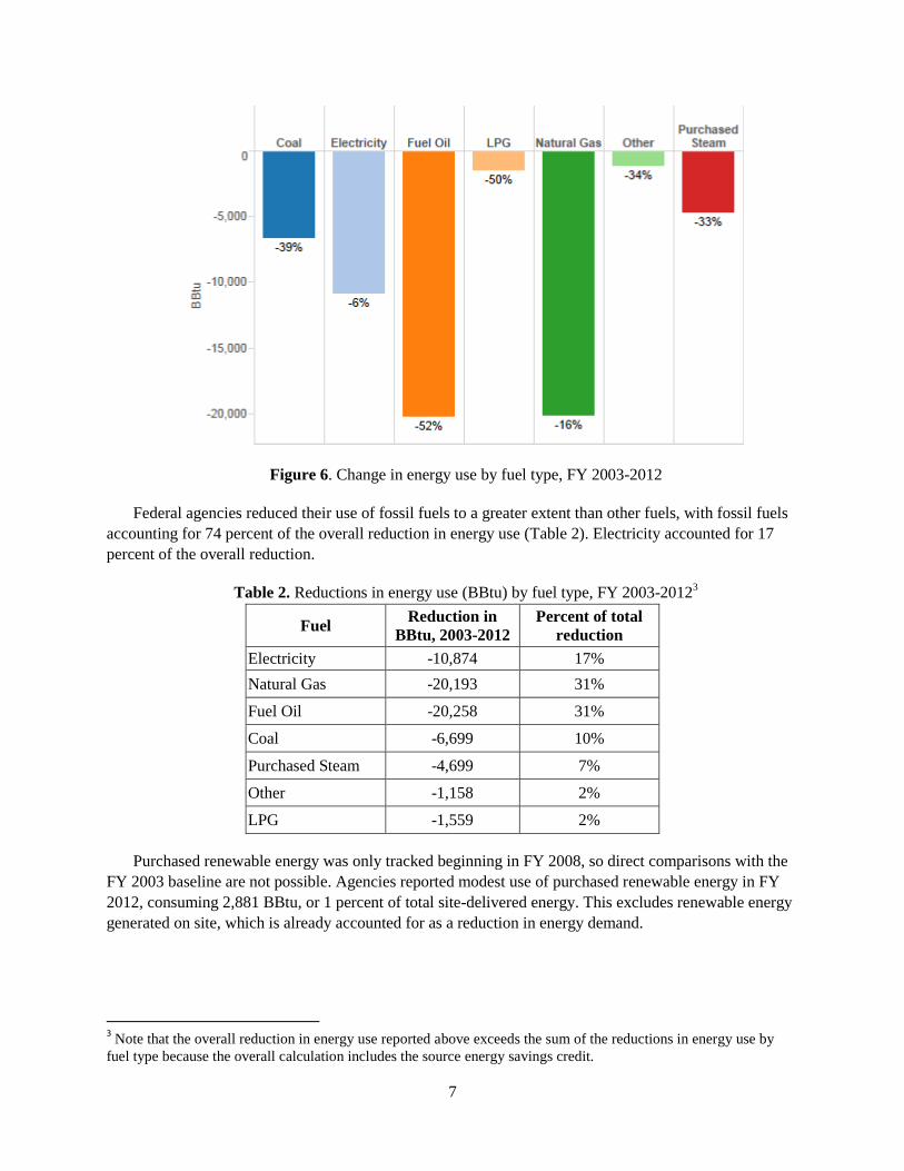
Figure 6. Change in energy use by fuel type, FY 2003-2012
Federal agencies reduced their use of fossil fuels to a greater extent than other fuels, with fossil fuels
accounting for 74 percent of the overall reduction in energy use (Table 2). Electricity accounted for 17
percent of the overall reduction.
Table 2. Reductions in energy use (BBtu) by fuel type, FY 2003-20123
Fuel Reduction in
BBtu, 2003-2012
Percent of total
reduction
Electricity -10,874 17%
Natural Gas -20,193 31%
Fuel Oil -20,258 31%
Coal -6,699 10%
Purchased Steam -4,699 7%
Other -1,158 2%
LPG -1,559 2%
Purchased renewable energy was only tracked beginning in FY 2008, so direct comparisons with the
FY 2003 baseline are not possible. Agencies reported modest use of purchased renewable energy in FY
2012, consuming 2,881 BBtu, or 1 percent of total site-delivered energy. This excludes renewable energy
generated on site, which is already accounted for as a reduction in energy demand.
3 Note that the overall reduction in energy use reported above exceeds the sum of the reductions in energy use by
fuel type because the overall calculation includes the source energy savings credit.

8
2.2 Agency-specific performance
As of FY 2012, 18 of 24 Office of Management and Budget (OMB) scorecard agencies4 had achieved
a reduction in energy intensity of 21 percent or greater. As shown in Table 3, three agencies—Department
of Justice (DOJ), Housing and Urban Development (HUD), and United States Postal Service (USPS)—
had already exceeded the 30 percent reduction goal. Four of the top five energy consuming agencies
(based on Figure 2) are on track to meet the 30 percent reduction goal in FY 2015 based on the 3 percent
annual reduction schedule outlined in Table 1, with DOD being the exception.
Table 3. Percent changes in EUI, total energy use, and floor space from FY 2003-2012
Agency
% Change in
Energy Intensity
(Btu/SF)
% Change in
Energy Use
(BBtu)
% Change in
Floor Space
(kSF) On Track?*
DHS -20.1% -5.9% +17.8% No
DOC -21.0% +43.9% +82.1% Yes
DOD -17.7% -15.2% +3.0% No
DOE -23.5% -28.9% -7.1% Yes
DOI -28.5% -13.4% +21.2% Yes
DOJ -44.6% -31.6% +23.5% Yes
DOL -28.1% -22.5% +7.8% Yes
DOT -23.9% -24.1% -0.2% Yes
EPA -23.7% -20.8% +3.8% Yes
GSA -24.5% -26.2% -2.2% Yes
HHS -22.4% -13.9% +10.9% Yes
HUD -33.1% -32.7% +0.6% Yes
NARA -27.3% +10.6% +52.0% Yes
NASA -23.9% -21.3% +3.4% Yes
OPM -2.7% -2.0% +0.7% No
SI -27.1% -0.5% +36.4% Yes
SSA -21.6% -29.6% -10.3% Yes
State -8.2% +11.0% +21.0% No
TRSY -11.8% -21.9% -11.4% No
TVA -21.2% -21.2% +0.0% Yes
USACE -11.4% -8.6% +3.2% No
USDA -21.3% -26.6% -6.7% Yes
USPS -32.4% -40.0% -11.4% Yes
VA -21.4% -7.6% +17.5% Yes
Total
Gov’t -20.6% -18.6% +2.6% Yes
*To meet 30% energy intensity reduction goal, according to FY 2012 OMB Sustainability/Energy
Scorecard.
4 Note that the energy performance requirement in 42 U.S.C. § 8253 applies specifically to agencies, not the federal
government as a whole.

9
In terms of overall energy consumption, floor space, and fuel mix, there were no clear trends
distinguishing agencies considered to be on track from those considered not on track. Agencies achieved
reductions in various ways. Among on-track agencies, the greatest reductions were achieved by agencies
whose total floor space increased while energy consumption decreased. DOJ, Department of the Interior
(DOI), VA, and Health and Human Services (HHS) demonstrated this trend. A notable exception is
USPS, which achieved the third-greatest reduction in energy intensity among all scorecard agencies,
decreasing floor space by 11 percent and energy use by 40 percent.
A majority of the agencies not on track also demonstrated reductions in energy consumption
accompanied by increased floor space. Among the scorecard agencies, State, Department of Commerce
(DOC), and National Archives and Records Administration (NARA) were the only three agencies whose
consumption increased, but in each case their square footage increased by a greater percentage, resulting
in an overall reduction in EUI.
When considering energy savings by fuel type, most agencies made large reductions in the use of fuel
oil. A majority of agencies also reduced their consumption of natural gas, and a similar number reduced
their electricity use. These trends were observed for agencies that are on-track to meet their EUI reduction
targets as well as those that are not on track.
Figure 7 illustrates the net reductions and increases in energy use by fuel type and by agency.
Observations on agency-level performance are presented below for several of the largest energy-
consuming agencies, including: DOD, DOE, HHS, DOJ, VA, GSA, and USPS.
Figure 7. Agency contribution to total energy savings by fuel type, FY 2003-2012

10
2.2.1 Department of Defense
In FY 2012, DOD used 96,593 Btu/SF in its goal-subject buildings. This represented a 17.7 percent
decrease in energy intensity compared to 117,334 Btu/SF in FY 2003. DOD is considered not on track to
meet the 30 percent reduction goal by OMB.
DOD’s total floor space has remained roughly constant since FY 2007, such that reductions in energy
use have resulted in corresponding reductions in energy intensity. DOD has only seen major reductions in
energy use over the most recent three fiscal years. Between FY 2003 and FY 2009, energy use decreased
by only 2.8 percent, setting DOD behind most other agencies (Figure 8).
Figure 8. DOD energy use intensity, energy use, and floor space for FY 2003-2012
Reductions have been achieved almost exclusively through decreased use of fossil fuels, which
accounts for 96 percent of the 32,539 BBtu of the decrease in all fuels since FY 2003. Use of fuel oil has
decreased most, both in relative and absolute terms, by 15,598 BBtu (a 50 percent decrease). Natural gas
use has also decreased substantially in absolute terms, by 9,797 BBtu (a 14 percent decrease). Coal and
LPG use have each decreased by more than one third. Because DOD’s energy use is so much higher than
the other agencies, these reductions have driven trends observed for the federal government as a whole.
For example, DOD accounted for 77 percent of the overall federal reduction in fuel oil use, and 80
percent of the overall reduction in coal use. DOD’s electricity use— its single largest source of energy
consumption— increased by 3 percent between FY 2003 and FY 2012, to 92,007 BBtu (Figure 9).

11
Figure 9. Change in DOD energy use by fuel type, FY 2003-2012
2.2.2 Department of Energy
In FY 2012, DOE used 170,301 Btu/SF in its goal-subject buildings. This represented a 24 percent
decrease in energy intensity compared to 222,472 Btu/SF used in FY 2003.
DOE’s floor space decreased by 20,292 thousand SF (kSF) between FY 2003 and FY 2008, but began
to increase again beginning in FY 2009. DOE’s energy use decreased relatively steadily each year over
the entire FY 2003-2012 period. At the end of the period, DOE’s floor space had decreased by only 7
percent, while energy use had declined by 29 percent (Figure 10).

12
Figure 10. DOE energy use intensity, energy use, and floor space for FY 2003-2012
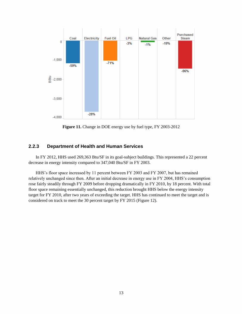
DOE’s performance in energy intensity reduction so far suggests that the agency will meet the
30 percent reduction target in or potentially before FY 2015. DOE achieved its reductions through
substantial decreases in the use of several fuels, including coal (1,176 BBtu, or 59 percent) and fuel oil
(1,046 BBtu, or 71 percent). DOE achieved the most dramatic reductions in energy use through a
28 percent decrease in electricity use, amounting to 3,668 BBtu. In addition, DOE reduced its use of
purchased steam by 96 percent (Figure 11).
13
Figure 11. Change in DOE energy use by fuel type, FY 2003-2012
2.2.3 Department of Health and Human Services
In FY 2012, HHS used 269,363 Btu/SF in its goal-subject buildings. This represented a 22 percent
decrease in energy intensity compared to 347,040 Btu/SF in FY 2003.
HHS’s floor space increased by 11 percent between FY 2003 and FY 2007, but has remained
relatively unchanged since then. After an initial decrease in energy use in FY 2004, HHS’s consumption
rose fairly steadily through FY 2009 before dropping dramatically in FY 2010, by 18 percent. With total
floor space remaining essentially unchanged, this reduction brought HHS below the energy intensity
target for FY 2010, after two years of exceeding the target. HHS has continued to meet the target and is
considered on track to meet the 30 percent target by FY 2015 (Figure 12).

14
Figure 12. HHS energy use intensity, energy use, and floor space for FY 2003-2012
HHS achieved its largest reductions in energy use through decreases in purchased steam of 1,216
BBtu (90 percent) and in fuel oil of 542 BBtu (70 percent). HHS reduced electricity use by 393 BBtu (11
percent). In addition, HHS completely eliminated its use of coal; however, this reduction did not have a
large impact on HHS’s overall energy use, as coal accounted for less than 1 percent of total energy use
throughout the FY 2003-2012 period. Unlike the other large scorecard agencies, all of which reduced
their use of natural gas, HHS’ use of natural gas actually increased substantially, by 2,235 BBtu, or 61
percent (Figure 13).

15
Figure 13. Change in HHS energy use by fuel type, FY 2003-2012
Since HHS’s reductions in energy use were largely offset by its increased use of natural gas, the
agency’s large reductions in energy intensity in the past three years were achieved primarily through the
application of the “renewable energy credit” and the “source energy credit” toward the Btu/SF
requirement.5 The credits amounted to 1,508 BBtu in FY 2010, or 82 percent of the total reduction in
energy reported for that year.
2.2.4 Department of Justice
In FY 2012, DOJ used 160,122 Btu/SF in its goal-subject buildings. This represented a 45 percent
decrease in energy intensity compared to 289,056 Btu/SF used in FY 2003.
DOJ’s floor space increased at a regular pace between FY 2003 and FY 2007, but has remained
relatively unchanged since FY 2008. Since FY 2007, its energy use dropped steadily each year,
decreasing by a total of 36 percent. That decrease resulted in a 33 percent drop in energy intensity over
the same period (Figure 14).
5 U.S. Department of Energy, Federal Energy Management Program. November 2012. Reporting Guidance for
Federal Agency Annual Report on Energy Management (per 42 U.S.C. 8258).

16
Figure 14. DOJ energy use intensity, energy use, and floor space for FY 2003-2012
In FY 2012, DOJ led all agencies in overall energy intensity reduction performance. DOJ was one of
three agencies to exceed the 30 percent reduction goal in advance of FY 2015. Its 45 percent reduction
was achieved almost completely through decreases in the use of natural gas and electricity. DOJ reduced
its natural gas consumption by 2,879 BBtu (a 34 percent decrease) and electricity use by 1,742 BBtu (a 25
percent decrease). In addition, DOJ reduced its use of purchased steam by 75 percent, or 515 BBtu
(Figure 15).

17
Figure 15. Change in DOJ energy use by fuel type, FY 2003-2012
2.2.5 Department of Veterans Affairs
In FY 2012, the VA used 154,085 Btu/SF in its goal-subject buildings. This represented a 21 percent
decrease in energy intensity compared to 196,025 Btu/SF used in FY 2003.
VA’s floor space decreased to a low of 142,271 kSF in FY 2006, and has increased each year since
then. The agency’s energy use has fluctuated on an annual basis but has trended downward overall over
the period FY 2003-2012, decreasing by 8 percent. The increase in floor space had a larger effect on VA’s
energy intensity than the decrease in energy use (Figure 16).

18
Figure 16. VA Energy Use Intensity, Energy Use, and Floor Space for FY 2003-2012
VA has met the energy intensity target for the past two years, and is considered on track to meet the
30 percent reduction target by FY 2015. VA achieved its largest energy use reductions in natural gas
(1,382 BBtu, or 9 percent) and fuel oil (964 BBtu, or 58 percent). VA also reduced its consumption of
LPG by 45 percent and coal by 34 percent, although these reductions had only a small effect on overall
energy use. These reductions were partially offset by an increase in electricity use of 1,042 BBtu, or 10
percent (Figure 17).

19
Figure 17. Change in VA energy use by fuel type, FY 2003-2012
Like HHS and GSA, VA made use of the Goal-Building Renewable Energy Credit and the Source
Energy Savings Credit to reduce its total calculated energy use. Energy use actually increased from FY
2011 to FY 2012, but after applying the Source Energy Savings Credit, VA’s total calculated energy use
in FY 2012 was 480 BBtu lower than the previous year.
2.2.6 General Services Administration
In FY 2012, GSA used 58,100 Btu/SF in its goal-subject buildings. This represented a 24 percent
decrease in energy intensity compared to 76,921 Btu/SF used in FY 2003.
GSA’s floor space and energy use increased dramatically between FY 2003-2004 and then fell back
to roughly FY 2003 levels in FY 2006. Between FY 2006 and FY 2009, floor space and energy use
remained essentially constant. Floor space has continued to stay fairly unchanged, while energy use began
to drop in FY 2010, falling 22 percent since FY 2009. The decreases in the previous three years account
for nearly all of GSA’s reduction against the FY 2003 baseline (Figure 18).
20
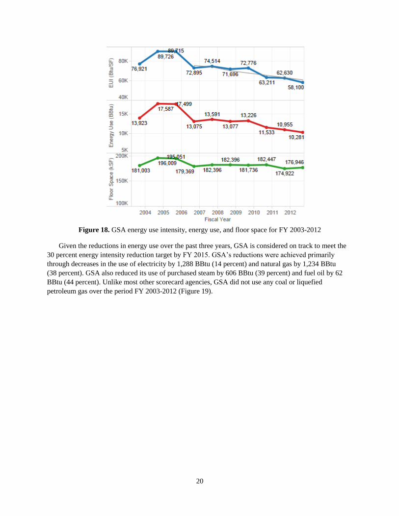
Figure 18. GSA energy use intensity, energy use, and floor space for FY 2003-2012
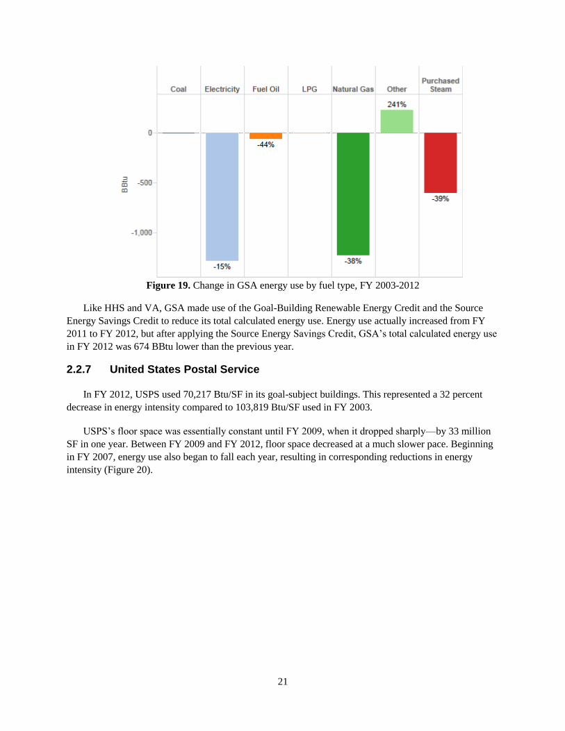
Given the reductions in energy use over the past three years, GSA is considered on track to meet the
30 percent energy intensity reduction target by FY 2015. GSA’s reductions were achieved primarily
through decreases in the use of electricity by 1,288 BBtu (14 percent) and natural gas by 1,234 BBtu
(38 percent). GSA also reduced its use of purchased steam by 606 BBtu (39 percent) and fuel oil by 62
BBtu (44 percent). Unlike most other scorecard agencies, GSA did not use any coal or liquefied
petroleum gas over the period FY 2003-2012 (Figure 19).
21
Figure 19. Change in GSA energy use by fuel type, FY 2003-2012
Like HHS and VA, GSA made use of the Goal-Building Renewable Energy Credit and the Source
Energy Savings Credit to reduce its total calculated energy use. Energy use actually increased from FY
2011 to FY 2012, but after applying the Source Energy Savings Credit, GSA’s total calculated energy use
in FY 2012 was 674 BBtu lower than the previous year.
2.2.7 United States Postal Service
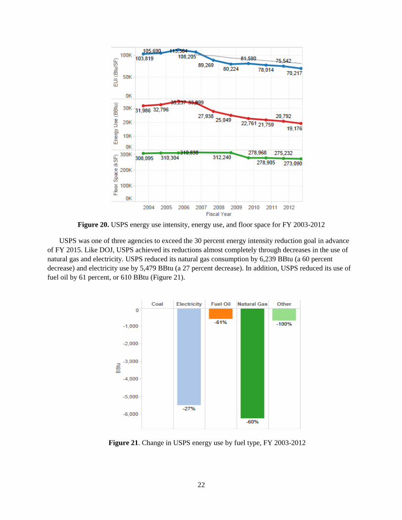
In FY 2012, USPS used 70,217 Btu/SF in its goal-subject buildings. This represented a 32 percent
decrease in energy intensity compared to 103,819 Btu/SF used in FY 2003.
USPS’s floor space was essentially constant until FY 2009, when it dropped sharply—by 33 million
SF in one year. Between FY 2009 and FY 2012, floor space decreased at a much slower pace. Beginning
in FY 2007, energy use also began to fall each year, resulting in corresponding reductions in energy
intensity (Figure 20).
22
Figure 20. USPS energy use intensity, energy use, and floor space for FY 2003-2012
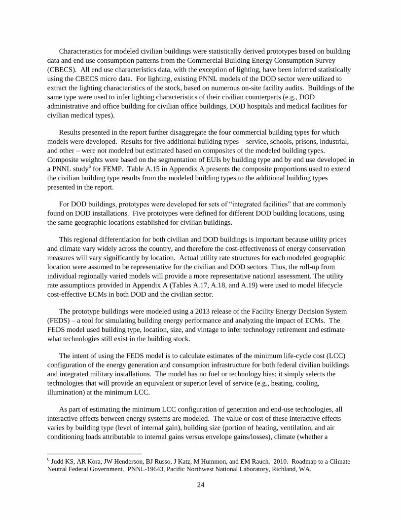
USPS was one of three agencies to exceed the 30 percent energy intensity reduction goal in advance
of FY 2015. Like DOJ, USPS achieved its reductions almost completely through decreases in the use of
natural gas and electricity. USPS reduced its natural gas consumption by 6,239 BBtu (a 60 percent
decrease) and electricity use by 5,479 BBtu (a 27 percent decrease). In addition, USPS reduced its use of
fuel oil by 61 percent, or 610 BBtu (Figure 21).
Figure 21. Change in USPS energy use by fuel type, FY 2003-2012

23
3.0 Future Energy Savings Potential in Federal Buildings
Future energy savings in federal buildings will be realized as a result of retrofits to existing buildings
as well as the retirement of old buildings and addition of newly constructed buildings that are designed to
much more efficient standards. This section examines the energy savings potential from both of these
sources. Section 3.1 presents the results of an analysis of potential energy savings that could be achieved
through investments in additional energy efficiency and renewable measures, while Section 3.2 presents
estimates of savings that would result from incorporating more energy efficient, newly constructed
buildings into the federal building stock.
This analysis is intended to convey the technical potential of investments in cost-effective energy
conservation measures (ECMs) and provides an estimated cost of implementing those measures in
existing buildings. The analysis is not intended to address policy, institutional, or other barriers to
implementing these ECMs, and makes no assumptions or projections about likely future funding levels.
However, the estimated costs of implementing these ECMs in different sectors and facilities described in
Section 3.1.4 may help inform budgetary requirements to realize the full energy savings potential.
The approach to estimating future savings potential is discussed briefly below and more detail on the
methodologies, modeling assumptions, and supporting calculations can be found in Appendices A, B, and
C.
3.1 Existing Building Retrofits
The objective of the building retrofit analysis was to estimate the potential energy savings that could
be achieved through further investments in lifecycle cost-effective energy efficiency measures in existing
federal buildings between 2016 and 2025, as well as the reduction potential from implementation of
renewable energy projects on federal buildings or sites. This analysis involved defining a set of prototype
buildings for the federal sector, modeling the impacts of energy efficiency retrofit and renewable energy
measures on these buildings, extrapolating results to the federal sector as a whole, and establishing
savings estimates, as is described below.
3.1.1 Modeling Prototype Federal Buildings
Prototype buildings were established to make sure that a representative sample of federal buildings
was modeled. Because of key differences in building characteristics and operations in DOD buildings and
civilian buildings, many of which are managed by the GSA, separate prototypes were established for the
civilian sector and for the DOD.
For the civilian sector, four building types were modeled: offices, warehouses, laboratories, and
hospitals. These represent the most common federal civilian building types in the U.S. as reported in the
Federal Real Property Profile (FRPP) database, and together these building types represent 66 percent of
civilian domestic floor area. Five building locations were also selected to reflect where the majority of
federal facilities are located based on the FRPP and to cover a mix of representative geographic and
climate regions (i.e., Washington, DC, Los Angeles, CA, Jacksonville, FL, New York, NY, and Dallas,
TX). Finally, different combinations of large/small and old/new buildings were established to represent
the current federal civilian building stock. Thirty variants of these civilian buildings were modeled in five
locations for a total of 150 model runs.
24
Characteristics for modeled civilian buildings were statistically derived prototypes based on building
data and end use consumption patterns from the Commercial Building Energy Consumption Survey
(CBECS). All end use characteristics data, with the exception of lighting, have been inferred statistically
using the CBECS micro data. For lighting, existing PNNL models of the DOD sector were utilized to
extract the lighting characteristics of the stock, based on numerous on-site facility audits. Buildings of the
same type were used to infer lighting characteristics of their civilian counterparts (e.g., DOD
administrative and office building for civilian office buildings, DOD hospitals and medical facilities for
civilian medical types).
Results presented in the report further disaggregate the four commercial building types for which
models were developed. Results for five additional building types – service, schools, prisons, industrial,
and other – were not modeled but estimated based on composites of the modeled building types.
Composite weights were based on the segmentation of EUIs by building type and by end use developed in
a PNNL study6 for FEMP. Table A.15 in Appendix A presents the composite proportions used to extend
the civilian building type results from the modeled building types to the additional building types
presented in the report.
For DOD buildings, prototypes were developed for sets of “integrated facilities” that are commonly
found on DOD installations. Five prototypes were defined for different DOD building locations, using
the same geographic locations established for civilian buildings.
This regional differentiation for both civilian and DOD buildings is important because utility prices
and climate vary widely across the country, and therefore the cost-effectiveness of energy conservation
measures will vary significantly by location. Actual utility rate structures for each modeled geographic
location were assumed to be representative for the civilian and DOD sectors. Thus, the roll-up from
individual regionally varied models will provide a more representative national assessment. The utility
rate assumptions provided in Appendix A (Tables A.17, A.18, and A.19) were used to model lifecycle
cost-effective ECMs in both DOD and the civilian sector.
The prototype buildings were modeled using a 2013 release of the Facility Energy Decision System
(FEDS) – a tool for simulating building energy performance and analyzing the impact of ECMs. The
FEDS model used building type, location, size, and vintage to infer technology retirement and estimate
what technologies still exist in the building stock.
The intent of using the FEDS model is to calculate estimates of the minimum life-cycle cost (LCC)
configuration of the energy generation and consumption infrastructure for both federal civilian buildings
and integrated military installations. The model has no fuel or technology bias; it simply selects the
technologies that will provide an equivalent or superior level of service (e.g., heating, cooling,
illumination) at the minimum LCC.
As part of estimating the minimum LCC configuration of generation and end-use technologies, all
interactive effects between energy systems are modeled. The value or cost of these interactive effects
varies by building type (level of internal gain), building size (portion of heating, ventilation, and air
conditioning loads attributable to internal gains versus envelope gains/losses), climate (whether a
6 Judd KS, AR Kora, JW Henderson, BJ Russo, J Katz, M Hummon, and EM Rauch. 2010. Roadmap to a Climate
Neutral Federal Government. PNNL-19643, Pacific Northwest National Laboratory, Richland, WA.
25
particular building is cooling- or heating-dominated), occupancy schedule, and a number of other factors.
Thus, there is no simple solution, and detailed simulation modeling is the best way to provide a credible
estimate of the impact. For example, when considering a lighting retrofit, the model evaluates the change
in energy consumption in all building energy systems rather than just the change in the lighting energy. In
addition, it was conservatively assumed that both sectors could achieve an additional 5 percent savings
through improved operations and continuous commissioning activities. See Appendix A for more detail
on the FEDS model assumptions.
The analyses yielded a life-cycle-cost-effective mix of ECMs, which resulted in estimated EUIs for
each of the prototype buildings and locations if all of the retrofits were implemented.
3.1.2 EUIs for Prototype Buildings
The federal building prototypes that were modeled produced target EUI estimates, which were
extrapolated to all floor area of a similar type in the civilian and DOD sectors. No distinction between
goal-subject and excluded buildings was made in the model, as there would be no reliable basis for
establishing prototypes that would exclude floor area not subject to efficiency goals. For building types
in the civilian sector that were not modeled, weighted-average EUIs were established using federal EUI
estimates by building type and location. The approach for developing all weighting and scaling of model
results to national estimates is discussed in Appendix A.
The results of the FEDS modeling were weighted and scaled such that the baseline EUI values were
consistent with relative values estimated using floor area based on the FRPP data. Regional weights were
developed also based on summarization of gross floor area from the FRPP data. The research team
assumed that the regional distribution of floor area or the distribution of floor area by building type would
not vary significantly during the 2016-2025 period.
Modeled EUI and total energy consumption estimates for civilian prototype buildings were based on
prototypes that PNNL has developed for related assessments. PNNL has completed site-specific energy
efficiency audits and analyses using FEDS for numerous military installations, which were used to
represent the DOD stock. The building-level data utilized in the FEDS model have been calibrated based
on the detailed facility audits of actual buildings. The estimates for the civilian sector buildings have
been developed based on representative composite buildings developed to provide statistically
representative average conditions based on segmentation by size, vintage, type, and technology
mix. Auditing a set of typical federal civilian buildings was beyond the scope of this study.
Model results were vetted with FEMP and agency personnel, and compared to actual federal building
energy performance data when available. Baseline EUIs were based on current reported civilian and
DOD values of 109 kBtu/SF for civilian buildings and 97 kBtu/SF for DOD buildings. These values were
adjusted to their 2015 starting values by extending the current trend of EUI goal progress over the 2003-
2012 period to the 2011-2015 period to bring the FEDS model starting EUIs in line with published
values. This resulted in 2015 starting values of 97.3 kBtu/SF for civilian buildings and 91.0 kBtu/SF for
DOD buildings.

26
3.1.3 Estimated Energy Savings Potential from Energy Conservation and
Efficiency
The estimated EUI impact results for existing buildings appear in Table 4. Results are presented in
site energy terms, which reflect the amount of energy use at the building meter.
Table 4. Estimated EUI impact of cost-effective energy conservation measures (site energy basis)
Sector and Building Type 2015 EUI
2025 EUI Reduction with
Efficiency Only 2025 EUI
kBtu/SF kBtu/SF Pct. kBtu/SF
All Civilian 97.3 10.9 11.2% 86.3
Civ: Healthcare 151.9 15.9 10.5% 135.9
Civ: Industrial 98.7 10.5 10.6% 88.2
Civ: Laboratory 145.0 13.6 9.4% 131.5
Civ: Office 92.0 10.6 11.5% 81.4
Civ: Prison 129.1 13.5 10.5% 115.5
Civ: School 73.8 9.2 12.5% 64.6
Civ: Service 68.3 8.8 12.8% 59.5
Civ: Warehouse 27.1 5.6 20.7% 21.5
Civ: Other 84.1 10.0 11.9% 74.1
All DOD 91.0 20.4 22.5% 70.6
All Federal 93.1 18.5 19.9% 74.5
The results suggest that if all cost-effective ECMs were deployed into the existing stock, then by
2025, a 20 percent reduction in EUI would be possible for the federal government as a whole from 2015.
Most of this potential arises from DOD facilities, which have an estimated EUI reduction potential of 22
percent, whereas the civilian sector has an estimated EUI improvement of 11 percent, based on
implementation of cost-effective ECMs. The actual savings potential could vary widely by agency, as
indicated by the variability in actual savings achieved to date and demonstrated in the analysis of past
performance.
Based on the information available for the modeling and analysis included in this report, the larger
energy-savings potential in DOD facilities compared to the civilian sector may be attributed to the age of
the DOD building stock and the progress toward the EUI reduction goal to date. The DOD sector has
achieved a 17.7 percent reduction from its 2003 baseline, while the civilian sector has reduced energy use
intensity 24.5 percent below its baseline (Table 5). One reason for the higher civilian EUI reductions may
be that the civilian sector as a whole has invested comparatively more into building efficiency than DOD
during the goal period. Between 2005 and 2013 DOD’s ratio of efficiency investment–to-energy costs (18
percent) is somewhat lower than the civilian sector’s ratio (33 percent including GSA, and 22 percent
excluding GSA, which has had higher than usual investment levels due to ARRA funding).
Furthermore, much more floor area in DOD is significantly less energy efficient than the floor area in
the federal civilian buildings when comparing a similar mix of building types. The DOD stock is older
and was not, until the last decade or so, built to the same standards. For example, uninsulated metal-sided
and metal-roofed buildings constructed for unoccupied and unconditioned storage have been repurposed
to heated, occupied warehousing. Wood-framed unconditioned office space (1940’s era) has since been
adapted with window-mount air conditioning and space heaters. This may explain in part the lower
starting EUIs and challenge associated with reducing them further. Such examples lead to significant

27
retrofit opportunities for envelope measures that increase insulation and reduce heating and cooling loads.
Other factors driving the comparatively lower rate of EUI reduction in DOD could be that DOD space has
become more highly utilized with the increased mission tempo and troops redeploying from overseas
missions to U.S facilities.
Table 5. Differences in progress toward current federal reduction targets for DOD and civilian agencies
Sector 2003 Baseline
EUI (kBtu/SF)
2012 Reported
EUI (kBtu/SF)
Percent
Reduction as of
2012
Projected 2015 EUI if
30% Goal is Met
(kBtu/SF)
Estimated 2015
EUI per Model
(kBtu/SF)
DOD 117.3 96.6 17.7% 82.1 91.0
Civilian 144.0 108.7 24.5% 100.8 97.3
3.1.4 Estimated Renewable Energy Production Potential
In addition to the modeling of cost-effective ECMs, this study also considers the additional impact
that developing technically feasible onsite renewable energy supplies would have on the building’s
overall EUI. Assessment of lifecycle cost-effectiveness of renewable energy requires site-level analysis
and was not feasible for this study of government-wide renewable energy potential. Furthermore, the
economics of future investments in renewable energy are largely driven by future pricing of renewables
and availability of tax credits and incentives, both of which pose a great deal of uncertainty. Therefore the
estimates presented in this section represent an upper limit of government-wide renewable production
potential.
To establish the technically feasible capacity of renewable energy on civilian buildings, renewable
capacity was sized such that for every hour of the year the output from the installed wind and PV would
not exceed the building energy demand that occurred during that hour. Thus, there is no hour during the
year that the building or installation would sell power back to the grid. This is a conservative assumption
and was used to deal with uncertainty around the potential for net metering at federal locations. It
represents capacity well below technical production potential. For DOD facilities, alternative
configurations of onsite wind and PV were modeled for optimum electricity output, also subject to the
constraint that renewable output would not exceed the facility energy demand in any hour. See Appendix
A for more discussion.
Based on this analysis, renewable energy production has the potential to further reduce EUIs in
civilian buildings by up to 4.1 percent over the proposed 2015 to 2025 goal period, as illustrated in Table
6. It is estimated that renewable energy production in DOD facilities has the potential to further reduce
facility EUI by up to 8.9 percent over the ten-year goal period. This appears to be roughly consistent with
estimates described in the DOD’s Sustainability Performance Report FY 2013, which states that DOD is
currently acquiring 9.6 percent of its energy from renewable sources and expects to achieve a target of 25
percent renewable energy by 2025, as required by Title 10, United States Code §2911(e)(2).7
As noted above, when setting government-wide reduction goals it should be considered that some of
this potential may not be cost-effective or practical to implement upon further analysis. For example, the
in the DOD’s Sustainability Performance report it is noted that, “One factor dampening the amount of
renewable energy the Department can report is its mission-driven decision to focus more resources on
7 Department of Defense Sustainability Performance Report FY 2013. Aug 13, 2013. Pp. 33.

28
increasing renewable energy capacity on DOD property, and fewer on purchasing renewable energy
credits.”8
Table 6. Potential 2015-2025 EUI reduction from implementing technically feasible onsite renewable
energy (site energy basis)
Sector and Building Type
Potential 2015- 2025 EUI Reduction with
Onsite Renewables
kBtu/SF Pct.
All Civilian 4.0 4.1%
Civ: Healthcare 3.8 2.5%
Civ: Industrial 5.2 5.3%
Civ: Laboratory 7.8 5.4%
Civ: Office 4.0 4.3%
Civ: Prison 3.2 2.5%
Civ: School 3.2 4.3%
Civ: Service 2.9 4.3%
Civ: Warehouse 1.2 4.3%
Civ: Other 3.6 4.3%
All DOD 8.1 8.9%
All Federal 6.5 6.9%
DOD has double the capacity to install onsite renewables compared to the civilian sector for a few
reasons. DOD sites have larger land area available for onsite renewables than do civilian buildings, which
were assumed to be constrained by the building roof area for PV. In its FY 2013 Sustainability
Performance Report, DOD states that it intends to accelerate the development of large-scale renewable
projects on their lands, and that each of the three Military Departments set a goal to install one gigawatt of
renewable energy on their installations: Air Force by 2016, Navy by 2020, and Army by 2025.9 Also,
DOD renewable potential considered both wind and PV whereas only PV was considered for civilian
buildings. Finally, the shape of the DOD profile with more evening and weekend loads from barracks and
family housing is more conducive to renewables under the “no net generation constraint” that the model
applied (i.e. sites were assumed to produce no more than there demand in light of net metering
uncertainties).
3.1.5 Estimated Cost of Implementation
Using the FEDS database of ECMs, the model selected for implementation in the existing stock
those measures that would be life-cycle cost-effective under the established FEDS methodology.
Appendix A discusses the specific measures considered in the model. Table 7 summarizes the costs in
simple nominal payback terms by building type Civilian agencies would see slightly shorter paybacks,
depending on the type of building, while DOD facilities would see slightly longer paybacks. This
difference is driven largely by the differential in electricity and gas rates between the two sectors.
8 Ibid.
9 Department of Defense Sustainability Performance Report. Aug 14, 2013. Pp. ES-8.

29
Table 7 does not account for the impacts of onsite renewables. Given the variety of factors that affect
the installed costs of renewables, including existing rate structures, incentive programs, and
configurations, no attempt was made to assess cost-effectiveness. It is likely that the costs for onsite
renewables would be relatively higher per kilowatt-hour (kWh) of electricity and thus would extend the
paybacks reported for efficiency ECMs alone. In addition, due to the complexities mentioned, it is not
likely that all technically feasible onsite renewables would be cost-effective to develop.
Table 7. Nominal installed costs and associated energy cost savings
impacts from efficiency measures (current dollars)
Building Type Installed Cost ($/SF) Annual Savings ($/SF) Simple Payback (Yrs)
All Civilian 2.68 0.42 6.4
Civ: Healthcare 3.56 0.63 5.7
Civ: Industrial 1.78 0.44 4.1
Civ: Laboratory 2.38 0.63 3.8
Civ: Office 2.36 0.34 6.8
Civ: Prison 3.02 0.53 5.7
Civ: School 1.93 0.29 6.7
Civ: Service 1.81 0.27 6.7
Civ: Warehouse 0.85 0.14 6.1
Civ: Other 2.18 0.32 6.8
All DOD 2.59 0.36 7.1
All Federal 2.62 0.38 6.8
The total investment required when the installed cost per square foot of $2.62 is applied to the total
federal floor area of 3,167 million square feet would be approximately $8.3 billion for all federal
agencies. Over $5.0 billion would be required for DOD investment and over $3.3 billion would be
required for all other federal civilian agencies. Considering the current floor area distribution by space
type and installation cost per square foot, about $1.2 billion of the $3.3 billion of the civilian federal
investment would be directed toward office retrofits and over $340 million would go to healthcare facility
retrofits.
This $8.3 billion total investment equates to an average annual investment in energy efficiency of
roughly $830 million for all agencies over the ten-year goal period. Looking at historic average annual
investment might suggest this is feasible, however it should be considered that these were heavily
influenced by ARRA funding which will not be sustained into the future. Government-wide from FY
2005 through 2013 was $1.6 billion per year ($943 million for civilian agencies and $671 million for
DOD), with GSA’s ARRA funding contributing to the significantly higher average on the civilian side.
Prior to the first year of ARRA funding in FY 2009, funding levels were under $1 billion per year.
The total investment required assumes projects are funded directly by the agency and does not
account for third-party financing costs. An estimated 72 percent of energy efficiency and renewable
investments funded by agencies between 2005 and 2013 were funded directly by agencies; the remaining
projects were third-party financed through energy savings performance contracts (ESPCs) or utility
energy service contracts (UESCs). Use of third party financing varies significantly by agency so was not
built into this analysis. It should be assumed however, that due to different payback thresholds and higher
financing costs, some of the long-payback items that are cost-effective with direct appropriations, may not
30
occur under a third-party financing scenario, therefore the total investment and savings potential would be
somewhat lower.
This level of investment is expected to yield roughly $1.2 billion in annual savings, with $700 million
per year for DOD and $520 million per year for civilian agencies. The majority of annual savings in the
civilian sector would come from investments in offices ($180 million per year), laboratories ($63
million), and healthcare ($60 million). Note that these investment and savings values by building type are
approximations based on the proportion of total domestic floor area that each of these building types
represent, as reported in the FRPP database.
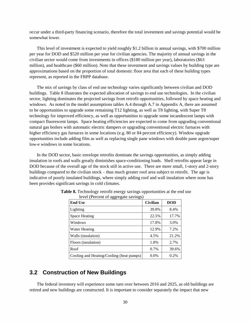
The mix of savings by class of end use technology varies significantly between civilian and DOD
buildings. Table 8 illustrates the expected allocation of savings to end use technologies. In the civilian
sector, lighting dominates the projected savings from retrofit opportunities, followed by space heating and
windows. As noted in the model assumptions tables A.4 through A.7 in Appendix A, there are assumed
to be opportunities to upgrade some remaining T12 lighting, as well as T8 lighting, with Super T8
technology for improved efficiency, as well as opportunities to upgrade some incandescent lamps with
compact fluorescent lamps. Space heating efficiencies are expected to come from upgrading conventional
natural gas boilers with automatic electric dampers or upgrading conventional electric furnaces with
higher efficiency gas furnaces in some locations (e.g. 80 or 84 percent efficiency). Window upgrade
opportunities include adding film as well as replacing single pane windows with double pane argon/super
low-e windows in some locations.
In the DOD sector, basic envelope retrofits dominate the savings opportunities, as simply adding
insulation in roofs and walls greatly diminishes space-conditioning loads. Shell retrofits appear large in
DOD because of the overall age of the stock still in active use. There are more small, 1-story and 2-story
buildings compared to the civilian stock – thus much greater roof area subject to retrofit. The age is
indicative of poorly insulated buildings, where simply adding roof and wall insulation where none has
been provides significant savings in cold climates.
Table 8. Technology retrofit energy savings opportunities at the end use
level (Percent of aggregate savings)
End Use Civilian DOD
Lighting 39.8% 8.4%
Space Heating 22.5% 17.7%
Windows 17.8% 3.0%
Water Heating 12.9% 7.2%
Walls (insulation) 4.5% 21.2%
Floors (insulation) 1.8% 2.7%
Roof 0.7% 39.6%
Cooling and Heating/Cooling (heat pumps) 0.0% 0.2%
3.2 Construction of New Buildings
The federal inventory will experience some turn over between 2016 and 2025, as old buildings are
retired and new buildings are constructed. It is important to consider separately the impact that new

31
buildings will have on the efficiency of the federal building stock because new federal buildings are
subject to more stringent design standards aimed at improving their energy performance. Specifically, the
2005 Energy Policy Act (EPAct 2005) requires that newly constructed federal buildings achieve 30
percent energy savings relative to the most recently published ASHRAE Standard 90.1.10
The objective of this analysis was to establish how requirements to adhere to new building efficiency
standards might impact energy performance of newly constructed federal buildings.
In the absence of data showing the impact that the current efficiency standards have had on new
building EUI performance to date, the methodology to estimate the impact of new building construction
on future EUI of federal buildings relies heavily on analyst judgment, but uses empirical data where it is
available. This involved first establishing the percentage of new building floor space that was likely to
comprise the federal building stock at the end of the goal-setting period (2025). Then, the difference in
the average EUIs of new buildings constructed during the goal period (2016-2025) was compared to the
expected EUI of the building stock at the beginning of the goal-setting period (2015). This approach is
described briefly below and in more detail in Appendix B.
3.2.1 Newly Constructed Floor Space
A simple model was developed to project the newly constructed floor space by considering the
amount of floor area that might be replaced (e.g., due to demolition, sale, or transfer) and an annual
growth of floor area that may be required to meet each agency’s mission. Annual disposal rates were
established for each major agency using disposal data reported in the FRPP for fiscal years 2006 through
2012 for civilian agencies. Data reported to FEMP was used to estimate USPS disposals as USPS does
not report its facilities in the FRPP. DOD floor area disposal estimates came from the DOD’s Base
Structure Report. These rates – along with an implied growth in total floor space projected to be the same
the U.S. population growth rate – were used to establish future disposals and potential new construction
estimates. These assumptions were vetted, and in a few cases modified, by the agencies.
The result of this analysis was an estimated amount of newly constructed floor area that would be
added between 2016 and 2025, and the percentage of the total federal building stock that the new
construction would represent in 2025. This was done for both goal-subject buildings as well as the entire
building stock (see “All Floor Area” in Table 9).
The columns highlighted in Table 9 are used to measure the impact of new energy-efficient buildings
on the EUIs of the total floor space stock in the year 2025. Based on the assumptions used, the civilian
sector (excluding USPS) is expected to see more new construction than the DOD. The much slower
growth rates in the overall stock for the USPS and the DOD will minimize the influence of new energy-
efficient, buildings on the overall intensity change over the next goal period of FY 2016-2025.
10
American Society of Heating, Refrigerating, and Air-Conditioning Engineers (ASHRAE). Major editions of non-
residential energy standards issued by ASHRAE were published in 1989, 1999, 2004, 2007, and 2010. The
standards are referenced as 90.1-year, where 90.1 is the standing ASHRAE committee dealing with energy
efficiency standards for nonresidential buildings.

32
Table 9. Floor space and new construction projections, FY 2016-2025 (millions of square feet)
Agency
2015 SF in
Inventory
(millions)
2025 SF in
Inventory
(millions)
Projected New Construction Additions to
Inventory
Goal-
Subject
Only
All
Floor
Area
Goal-
Subject
Only
All
Floor
Area
Goal-
Subject SF
Added
2016-2025
Pct. of
Goal-
Subject
SF in
2025
All SF
Added
2016-
2025
Pct. of
All SF in
2025
Civilian 880 989 940 1,056 149.0 16% 169.7 16%
DOE 102 118 106 122 16.1 15% 18.6 15%
GSA 181 213 196 231 36.2 18% 42.6 18%
DOJ 72 72 78 78 8.9 11% 8.9 11%
VA 183 183 197 197 19.5 10% 19.5 10%
USDA 59 59 62 62 13.0 21% 13.0 21%
DHS 48 49 52 53 11.8 23% 12.0 23%
DOI 60 60 63 63 11.3 18% 11.3 18%
NASA 33 40 35 42 3.8 11% 4.6 11%
All Other 142 196 151 209 28.3 19% 39.1 19%
USPS 271 271 265 265 4.0 1.5% 4.0 1.5%
Civilian & USPS 1,151 1,260 1,205 1,321 153.0 13% 174 13%
DOD 1,804 1,833 1,847 1,877 81.0 4% 82.3 4 %
All Federal 2,955 3,093 3,051 3,198 234.0 7.7% 256.0 8.0%
3.2.2 Impact of ASHRAE Standards and Other Factors on Newly Constructed
Building EUIs
To project what contribution the new, more efficient federal buildings constructed over the period
2016-2025 would have on the overall EUI of the federal building stock, the research team attempted to
quantify the influence of several individual factors that would influence the performance of newly
constructed buildings. These included:
1. The average EUI of the stock of buildings in the starting year of the goal setting period (2015)
2. The impact of the current ASHRAE Standard 90.1-2010 on new construction
3. The impact of a hypothetical future ASHRAE Standard 90.1-2016 on new construction
4. Requirements that new federal buildings must exceed energy efficiency improvements called for
in the ASHRAE 90.1 standards by 30 percent
5. Increased energy use in new buildings that results from greater utilization and higher electric plug
loads as compared to existing buildings.
First, to establish the baseline stock EUI, it was assumed that the current stock of buildings (and those
in 2015) could be characterized relative to buildings built to meet ASHRAE Standard 90.1-2004. A recent
DOE study to characterize the energy intensities of various vintages of all commercial buildings was used
to establish the EUI of the current stock of federal buildings. It was assumed that recently constructed
federal buildings built to ASHRAE 90.1-2004 would have an average EUI of about 10 percent below the
33
existing stock of buildings, as is shown in the first column of Table 10. (See Appendix B for further
discussion underlying this assumption.)
Second, the research team estimated the impact that the subsequent ASHRAE Standard 90.1-2010
would have on the EUIs of new federal buildings constructed to this standard. ASHRAE Standard 90.1-
2010 is the currently pending federal energy standard for new federal construction after July 9, 2014, so
will provide the basis for new construction at the beginning of the goal period. Based on a recent study by
PNNL (Thornton et al., 2011) on reductions in energy use between buildings built to the 90.1-2004 and
the 90.1-2010 editions of ASHRAE, it was assumed that buildings designed to ASHRAE Standard 90.1-
2010 will use about 24 percent less energy than those designed to ASHRAE Standard 90.1-2004. (See
“New Standard 90.1 Relative to 90.1-2004”, row 1 in Table 10.)
Third, the impact of future ASHRAE standards was considered. ASHRAE standards are typically
issued on a three-year cycle, therefore it is expected that at least one new standard will be issued between
2016 and 2025. While it is difficult to predict the stringency of the 90.1 Standard for each future cycle,
the research team attempted to account for the impact of future standards by positing a single step
increase in the federal building standard during the goal period. It was assumed a new standard issued by
the end of 2016 would become the baseline for federal new construction and begin having an impact on
buildings built after 2020, therefore would affect construction in the second half of the goal period.
A recent PNNL report suggests reductions of 7 percent over each three-year cycle of the Standard
90.1 based on historically observed efficiency improvements in the standard and expert judgment. This
would indicate a reduction of 14 percent in the overall EUI between the current standard 90.1-2010 and a
hypothetical 90.1-2016 standard.11
In light of the speculative nature of future standards, this analysis
takes as a conservative position and assumes the 2016 standard might reflect a 10 percent improvement
over the 90.1-2010 Standard. This 10 percent increase in the percentage savings results in a total
estimated savings of 34 percent compared to the 2015 base year stock EUI. (See “New Standard 90.1
Relative to 90.1-2004”, row 2 in Table 10.)
Fourth, the research team considered the impact of the 2005 EPAct requirement that newly
constructed federal buildings achieve an energy savings of 30 percent greater than the most recently
published ASHRAE Standard 90.1. The 30 percent target, however, is contingent on the additional energy
efficiency design features to be cost effective therefore that not all buildings will achieve this.
Furthermore, the energy standard for new federal building construction based on Standard 90.1-2010 will
start during 2014 which could make it more challenging to achieve the additional 30 percent improvement
in 2015. Because there is no basis for establishing compliance with the beyond ASHRAE requirement,
this analysis has taken a conservative position and assumes the average improvement beyond ASHRAE
will be only 10 percent. (See “Federal Design over Relevant Standard” in Table 10).
The fifth factor considered works in an opposing fashion to the previously discussed factors. There is
reason to believe that new commercial buildings could have a greater EUI on average than the existing
stock as new buildings will likely have higher utilization (hours of operation per week), higher occupant
density, and higher plug loads from growing density of computer equipment and servers in new buildings
11
This activity is part of PNNL’s support of DOE’s Building Energy Codes Program. PNNL is developing a cost-
effectiveness analysis of proposed changes in the 90.1 Standards, to be presented to ASHRAE and DOE by the end
of calendar 2013. When completed, this analysis will likely provide a more defensible basis for projecting
additional stringency in 90.1 over the next several cycles.

34
compared to existing buildings. The 2003 Commercial Building Energy Consumption Survey (CBECS)
provides some validation of this assumption. (See more detailed discussion in Appendix B). As a result,
the analysis here assumes that these factors might offset the increases in design efficiency by an average
15 percent. (See “Greater Energy Demand” in Table 10.)
Table 10. Impact of new construction meeting ASHRAE Standard 90.1-2010 and a hypothetical future
Standard 90.1-2016 on average building stock EUI in 2025
Standard 90.1-2004
Relative to
2015 Stock
New Standard
90.1 Relative
to 90.1-2004
Federal Design
over Relevant
Standard
Greater
Energy
Demand
Average EUI
Compared to
2015 Stock
EUI
(Reduction) (Reduction) (Reduction) (Increase) (Reduction)
90.1-2010 10% 24% 10% 15% 29%
90.1-2016 10% 34% 10% 15% 39%
Considering the collective impact of the five factors discussed above, the percentage difference
between the average EUI in new federal buildings built to the new ASHRAE standards and the EUI of the
2015 stock is estimated to be 29 percent for those built to 90.1-2010 and 39 percent for those built to
90.1-2016. This overall impact is calculated as a sum of the percentage changes in first four columns, and
by subtracting the increase in demand. (See last column of Table 10).
3.2.3 Impact on 2025 EUI of Federal Building Stock
The final step involved estimating the impact that new building construction has on the average EUI
of the 2025 federal building stock. First, the relative amount of floor space built under the two efficiency
standards discussed above was established. It was assumed that half of the new floor space constructed
between 2016 and 2025 is effectively built to meet the baseline ASHRAE Standard 90.1-2010 and the
other half meets the more stringent ASHRAE Standard 90.1-2016. The average reduction in EUI is then
assumed to be 34 percent (i.e., an average of values in the last column of Table 10).
The average expected reduction in EUI was then applied to the 13.1 percent of all newly constructed
floor space that civilian federal agencies were estimated to add to their building stock by 2015 (see “All
Civilian” in Table 9). The product of these two percentages (13.1% x 34%) yields a value of 4.5 percent
over the ten-year period. This reduction translates into an annual average reduction of approximately 0.4
percent (Table 11).
Table 11. Impact of new building construction on 2025 civilian stock EUI
Impact on Stock
EUI in 2025
(total % reduction)
Average Annual
Impact on EUI
(% reduction/year)
All Civilian 4.5% 0.4%
DOD 1.5% 0.2%
All Federal Agencies 2.7% 0.3%
The same type of calculation was performed for the military sector and for the total of all federal
buildings. As shown in Table 11, the smaller projected percentage of new construction for all military

35
buildings (4.4%) yields a lower impact on the overall EUI, estimated to be 1.5 percent. For the
combination of federal civilian and military categories, the new building impact is calculated to be 2.7
percent.
The values in Table 11 are shown as reflecting best judgment point estimates. Appendix B includes
estimates of “high” and “low” values that incorporate some informal uncertainty analysis pertaining to the
underlying elements of EUI reductions for new buildings.
The incremental impact for the new stock contribution reflects the assumed higher energy efficiencies
required by building codes and standards applicable to new construction. With time, as post-2015
construction becomes a larger share of the stock, natural improvement in the overall stock EUI will
continue. The values shown in Table 11 reflect the contribution of these factors in the terminal year of
this analysis, 2025.
3.3 Combined Impact of Retrofits and New Construction on Federal
Building Stock EUI
By the end of the goal period in 2025, the estimated federal stock total EUI reduction potential is 22.6
percent (see Table 12). That is the weighted average of the civilian improvement potential (15.7%) and
the potential in DOD facilities (24.0%).
Table 12. Estimated EUI impact from both cost-effective retrofits to existing buildings and federal
energy standards for new construction (site energy basis)
Building Type
Existing Buildings New
Buildings Total Stock
2015
EUI
2025 EUI
Reduction
(Efficiency Only)
2025
EUI
2025 EUI
Reduction 2025 EUI
kBtu/SF kBtu/SF Pct. kBtu /SF kBtu/SF kBtu/SF Pct. Change
All Civilian 97.3 10.9 11.2% 86.3 4.3 82.0 15.7%
Civ: Health Care 151.9 15.9 10.5% 135.9
Civ: Industrial 98.7 10.5 10.6% 88.2
Civ: Laboratory 145.0 13.6 9.4% 131.5
Civ: Office 92.0 10.6 11.5% 81.4
Civ: Prison 129.1 13.5 10.5% 115.5
Civ: School 73.8 9.2 12.5% 64.6
Civ: Service 68.3 8.8 12.8% 59.5
Civ: Warehouse 27.1 5.6 20.7% 21.5
Civ: Other 84.1 10.0 11.9% 74.1
DOD 91.0 20.4 22.5% 70.6 1.4 69.2 24.0%
Total Federal 93.1 18.5 19.9% 74.5 2.5 72.0 22.6%
As discussed in Section 3.1.4, some additional EUI reduction potential is likely feasible through
implementation of onsite renewable energy projects. Up to 4 percent and 9 percent is estimated to be
technically feasible in civilian and DOD buildings, respectively, over the ten-year goal period. Because

36
cost-effectiveness of renewable production projects can only be understood through site-level evaluations
and the economics are largely influenced by factors such as future technology pricing and availability of
state and federal incentives, there is a fair amount of uncertainty around the ability to exploit this potential
ten years from now. However this may provide an upper limit to what is feasible.
Finally, it should be emphasized that the EUI reduction potential presented in this study does not
represent a recommended reduction goal. These reflect a combined estimate of lifecycle cost-effective
retrofit measures, estimated reductions from replacing a relatively small amount of old floor space with
new, more efficient floor space, and a high-level estimate of technically feasible renewable projects.
These aim to provide a much more informed estimate of reduction potential, however it is recognized that
not all of the projects underlying these estimates may be practical or feasible to implement. Budgetary
constraints, organizational limitations, and operational preferences will all influence what can ultimately
be implemented. The cost estimates in section 3.1.5 are intended to illustrate the levels of funding that
would be required to achieve these EUI values. The influence of other agency factors, such as availability
of staffing resources for maintenance and operations of these systems, cannot be anticipated as part of this
study, but should be considered when setting specific goals.
4.0 Alternative Energy Performance Evaluation Approaches
Defining the best performance evaluation approach ultimately depends on what policymakers and the
federal government want to accomplish with energy management. The National Energy Conservation
Policy Act (NECPA), which serves as the underlying authority for current federal energy management
goals, states the purpose of federal energy management as broadly promoting “the conservation and the
efficient use of energy and water, and the use of renewable energy sources, by the Federal
Government.”12
The NECPA also cites benefits of increased energy efficiency as reducing the cost to
government, reducing dependence on foreign energy sources, and demonstrating the benefits of energy
efficiency to the nation. This suggests that energy use reduction, operational efficiency, cost savings,
energy supply security, and technology demonstration are all important outcomes from this policy.
The current metric established in the NECPA (as amended by EISA 2007) and adopted by the federal
government is EUI using site-delivered energy and a 2003 baseline year. While not perfect, EUI is
reasonable measure of the energy management goal outlined in the NECPA. It can be implemented in
many different ways however. In the section below, different approaches to setting EUI targets and
baseline years are considered. In addition, some alternative approaches are presented that may offer more
accurate measures of energy performance, environmental impacts, and/or ancillary benefits, such as cost
savings.
The primary options evaluated included:
Using site versus source EUI as the performance metric
Including only goal-subject versus all federal buildings
Using 2003 and alternative baseline years
12
42 USC § 8251.
37
Establishing a single federal target versus agency- or sector-specific targets
Establishing intensity versus absolute reduction goals
4.1 Site vs. Source EUI
4.1.1 Description of Source Energy Calculations
Agencies currently report EUI performance using site energy as a basis for the calculation. Site
energy refers to the amount of heat input and electricity delivered to a building and consumed as reflected
at the meter. In contrast, source energy refers to the total amount of raw fuel that is required to operate the
building, including all transmission, delivery, and losses associated with the production of secondary
energy products, such as purchased electricity and heat from district steam. In the 1980s, energy reduction
goals were established as source energy,13
but since then agency energy performance has been evaluated
on a site energy basis.
FEMP is considering using a modified source energy factor—referred to here as fossil-source
energy—as a basis for evaluating agency energy performance in the future. Whereas source energy
considers the heat input of all fuels (renewable and non-renewable), fossil-source energy accounts for the
heat input of only the raw fossil fuels required to operate a building and excludes the heat input from non-
greenhouse gas emitting energy resources including hydropower, nuclear power, and non-combustible
renewables. The benefits and drawbacks of each approach are discussed below, followed by an
illustration of the impact these factors would have on past and projected future energy performance.
Fossil-source energy EUI is calculated the same as site energy except that the amounts of purchased
electricity and steam are increased to reflect total primary energy use at the generation plant.14
Because
the total primary energy consumed is greater than the energy consumed on site, EUI calculated using
source energy is always larger than EUI calculated using site energy. Furthermore, the amount of primary
fossil energy required varies from site to site based on the fuel mix of the eGRID subregion that the
building draws from. By dividing heat input at the generation plant by net generation, a set of primary
energy conversion factors can be calculated for each subregion and applied to on-site electricity
consumption to determine total source energy. Alternatively, a national primary energy conversion factor
can also be derived.
The national fossil energy factor applied to all electricity consumed by federal agencies is 1.98 using
the most recent eGRID summary data for the U.S. Table 13 below shows fossil-source energy factors by
eGRID subregion. Variation in fossil-intensity by eGRID region can be viewed in the heat map in
Appendix D.
13
In the Annual Report to Congress on Federal Government Energy Management for FY 1989, electricity was
reported as total source energy using a conversion factor of 11,600 Btu/kWh. Starting in FY 1990, electricity use
was reported to Congress as site energy, using a conversion factor of 3412 Btu/kWh. 14
For simplicity, a transmission and distribution loss factor is not included in the calculation of the fossil source
energy factor, because such a factor would have no impact on the final calculation of percent change in EUI.

38
Table 13. Fossil-source energy using regional eGRID factors
Subregion FY 2008 FY 2012 Subregion FY 2008 FY 2012
AKGD 2.81 2.77 NYLI 2.98 2.97
AKMS 1.02 0.98 NYUP 1.18 0.92
AZNM 2.15 2.04 RFCE 1.67 1.55
CAMX 1.57 1.53 RFCM 2.56 2.48
ERCT 2.25 2.11 RFCW 2.27 2.19
FRCC 2.26 2.26 RMPA 2.98 2.80
HIMS 2.48 2.47 SPNO 2.68 2.64
HIOA 2.78 2.75 SPSO 2.75 2.64
MROE 2.59 2.34 SRMV 2.02 1.94
MROW 2.53 2.32 SRMW 2.6 2.46
NEWE 1.78 1.60 SRSO 2.34 2.15
NWPP 1.38 1.32 SRTV 2.31 2.02
NYCW 1.67 1.46 SRVC 1.72 1.62
Note that, using the eGRID source calculation methodology, electricity generated using geothermal,
hydropower, nuclear, wind, or solar sources is assigned a heat input of zero. As a consequence, regions
such as upstate New York (NYUP), where hydropower and nuclear comprise more than 60 percent of
generating capacity, have comparatively low fossil-source energy factors.
4.1.2 Benefits and Drawbacks
Table 14 summarizes some of the trade-offs between using site and source energy as the basis for
measuring EUI reduction performance.
Site energy has the benefit of being consistent with the current approach to performance evaluation.
Site energy also provides a more useful gauge of the impact of ECMs implemented at the site level to
save energy, as it isolates site energy use from changes in the generation mix at the regional or national
level. Since changes in the fossil-fuel intensity of the generation mix can drive total source energy
consumption (and therefore source EUI) up or down independently of facility energy management
decisions, using source energy to calculate EUI may obscure the effects of agency actions to improve
building energy efficiency. However, it should be noted that agencies would likely continue reporting
energy use in site-delivered terms, so both factors could be derived and used for different purposes.
Furthermore, other sources of federal energy data reporting (i.e., the Compliance Tracking System) are
available to provide a measure of the impact of ECMs implemented at the facility level.
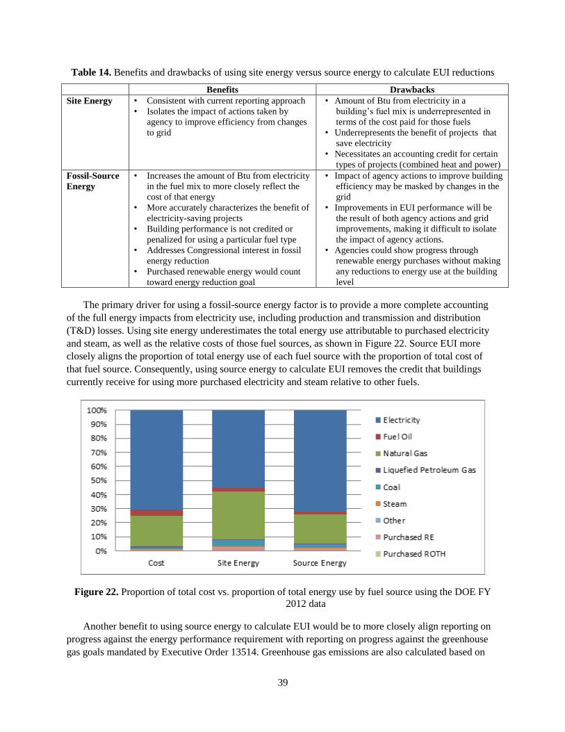
39
Table 14. Benefits and drawbacks of using site energy versus source energy to calculate EUI reductions
Benefits Drawbacks
Site Energy • Consistent with current reporting approach
• Isolates the impact of actions taken by
agency to improve efficiency from changes
to grid
• Amount of Btu from electricity in a
building’s fuel mix is underrepresented in
terms of the cost paid for those fuels
• Underrepresents the benefit of projects that
save electricity
• Necessitates an accounting credit for certain
types of projects (combined heat and power)
Fossil-Source
Energy
• Increases the amount of Btu from electricity
in the fuel mix to more closely reflect the
cost of that energy
• More accurately characterizes the benefit of
electricity-saving projects
• Building performance is not credited or
penalized for using a particular fuel type
• Addresses Congressional interest in fossil
energy reduction
• Purchased renewable energy would count
toward energy reduction goal
• Impact of agency actions to improve building
efficiency may be masked by changes in the
grid
• Improvements in EUI performance will be
the result of both agency actions and grid
improvements, making it difficult to isolate
the impact of agency actions.
• Agencies could show progress through
renewable energy purchases without making
any reductions to energy use at the building
level
The primary driver for using a fossil-source energy factor is to provide a more complete accounting
of the full energy impacts from electricity use, including production and transmission and distribution
(T&D) losses. Using site energy underestimates the total energy use attributable to purchased electricity
and steam, as well as the relative costs of those fuel sources, as shown in Figure 22. Source EUI more
closely aligns the proportion of total energy use of each fuel source with the proportion of total cost of
that fuel source. Consequently, using source energy to calculate EUI removes the credit that buildings
currently receive for using more purchased electricity and steam relative to other fuels.
Figure 22. Proportion of total cost vs. proportion of total energy use by fuel source using the DOE FY
2012 data
Another benefit to using source energy to calculate EUI would be to more closely align reporting on
progress against the energy performance requirement with reporting on progress against the greenhouse
gas goals mandated by Executive Order 13514. Greenhouse gas emissions are also calculated based on

40
the fossil-intensity of the grid using eGRID factors. As the overall fossil intensity of the grid decreases,
agencies would benefit from this as well.
Finally, the use of a fossil-source energy scenario would change the rules regarding accounting for
purchased renewable energy. While purchased renewable energy (i.e., Renewable Energy Certificates)
does not currently count toward the EUI reduction goal using site energy, these purchases would count
toward the EUI goal under the fossil-source energy scenario. If the electricity purchased by the agency is
not coming from a fossil source, its source energy would have a factor of zero. The drawback to this
approach is that an agency could actually increase electricity consumption significantly at the building
level and still show an EUI reduction through purchases of renewable electricity.
As noted above, a fossil-source energy factor can be derived using a national average factor or using
regional factors specific to the fuel mix in each eGRID subregion. Use of each of these approaches has its
own advantages and disadvantages as summarized in Table 15. Use of a national factor offers the benefit
of simplicity; a single factor is used regardless of the location of the agency’s facilities. On the other
hand, using a national factor may provide less incentive for agencies to direct energy-saving investments
into the most fossil-intensive regions (although in theory greenhouse gas emission goals would still
provide this incentive). Using a regional factor may provide an additional incentive to make efficiency
investments where it matters most (i.e., in the most fossil-fuel intensive regions) and provides a more
accurate estimate of each building’s energy use based on the predominant fuels used to generate
electricity in the building’s region. While EUI using regional factors will be slightly more complex for
agencies to calculate, at the federal level the current energy reporting structure for greenhouse gas
emissions calculations already maps to eGRID subregions, so there would be additional reporting
requirements.
Table 15. Benefits and drawbacks of using national versus regional source energy factors to
calculate EUI reductions
Benefits Drawbacks
National Factors • Provides a single, consistent factor
for all agencies and locations
• Similar to the U.S. Environmental
Protection Agency’s (EPA’s) Energy
Star Portfolio Manager methodology,
which uses a national non-fossil
source factor for benchmarking
• No additional benefit from reductions
in more fossil-fuel-intensive regions
• Improvements in energy performance
are determined in part by factors
outside of the agency’s control
Regional Factors • Rewards agencies for reductions in
more fossil-energy-intensive
locations
• More accurately reflects total fossil
energy use based in the building’s
region
• More complex to calculate
• Each agency will have a unique factor
based on building locations, which
will vary over time
• Improvements in energy performance
are determined in part by factors
outside of the agency’s control
To establish how using site versus fossil-source energy might influence agency goals, the research
team examined the impact that using a source energy factor percentage would have had on past federal
building energy performance as well as the savings potential from future retrofits, as discussed below.
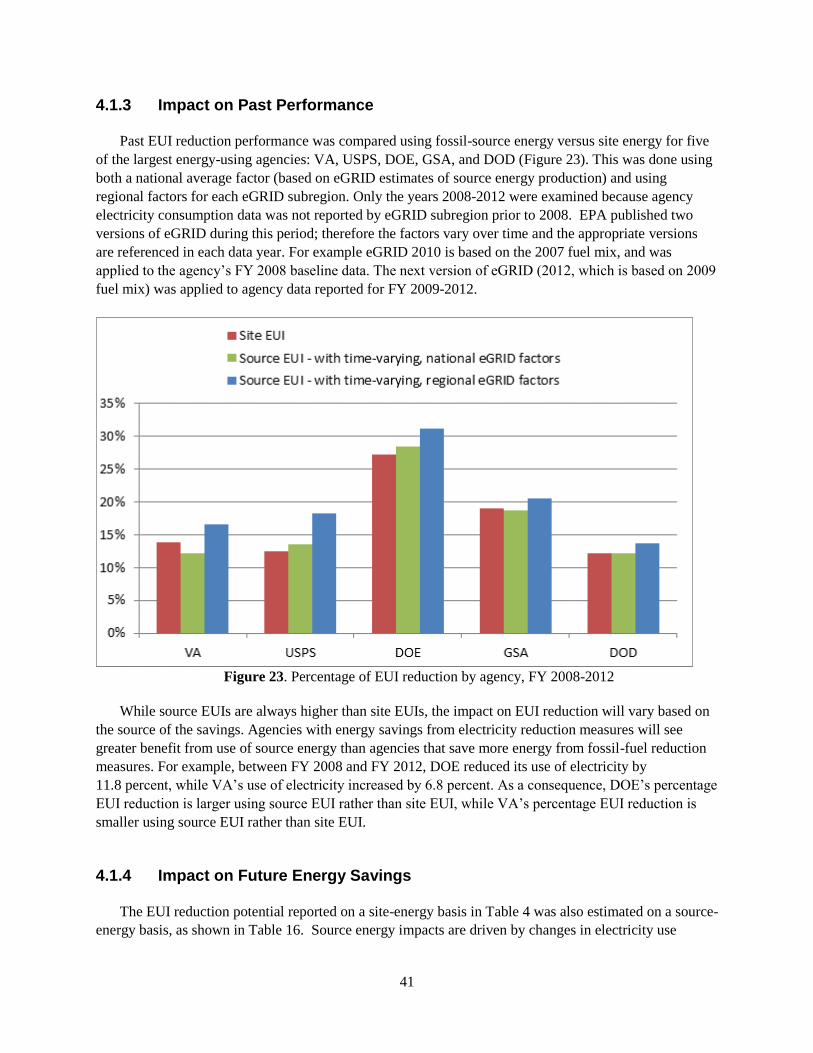
41
4.1.3 Impact on Past Performance
Past EUI reduction performance was compared using fossil-source energy versus site energy for five
of the largest energy-using agencies: VA, USPS, DOE, GSA, and DOD (Figure 23). This was done using
both a national average factor (based on eGRID estimates of source energy production) and using
regional factors for each eGRID subregion. Only the years 2008-2012 were examined because agency
electricity consumption data was not reported by eGRID subregion prior to 2008. EPA published two
versions of eGRID during this period; therefore the factors vary over time and the appropriate versions
are referenced in each data year. For example eGRID 2010 is based on the 2007 fuel mix, and was
applied to the agency’s FY 2008 baseline data. The next version of eGRID (2012, which is based on 2009
fuel mix) was applied to agency data reported for FY 2009-2012.
Figure 23. Percentage of EUI reduction by agency, FY 2008-2012
While source EUIs are always higher than site EUIs, the impact on EUI reduction will vary based on
the source of the savings. Agencies with energy savings from electricity reduction measures will see
greater benefit from use of source energy than agencies that save more energy from fossil-fuel reduction
measures. For example, between FY 2008 and FY 2012, DOE reduced its use of electricity by
11.8 percent, while VA’s use of electricity increased by 6.8 percent. As a consequence, DOE’s percentage
EUI reduction is larger using source EUI rather than site EUI, while VA’s percentage EUI reduction is
smaller using source EUI rather than site EUI.
4.1.4 Impact on Future Energy Savings
The EUI reduction potential reported on a site-energy basis in Table 4 was also estimated on a source-
energy basis, as shown in Table 16. Source energy impacts are driven by changes in electricity use
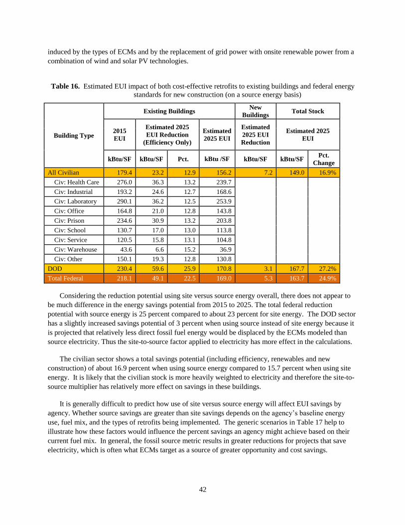
42
induced by the types of ECMs and by the replacement of grid power with onsite renewable power from a
combination of wind and solar PV technologies.
Table 16. Estimated EUI impact of both cost-effective retrofits to existing buildings and federal energy
standards for new construction (on a source energy basis)
Building Type
Existing Buildings New
Buildings Total Stock
2015
EUI
Estimated 2025
EUI Reduction
(Efficiency Only)
Estimated
2025 EUI
Estimated
2025 EUI
Reduction
Estimated 2025
EUI
kBtu/SF kBtu/SF Pct. kBtu /SF kBtu/SF kBtu/SF Pct.
Change
All Civilian 179.4 23.2 12.9 156.2 7.2 149.0 16.9%
Civ: Health Care 276.0 36.3 13.2 239.7
Civ: Industrial 193.2 24.6 12.7 168.6
Civ: Laboratory 290.1 36.2 12.5 253.9
Civ: Office 164.8 21.0 12.8 143.8
Civ: Prison 234.6 30.9 13.2 203.8
Civ: School 130.7 17.0 13.0 113.8
Civ: Service 120.5 15.8 13.1 104.8
Civ: Warehouse 43.6 6.6 15.2 36.9
Civ: Other 150.1 19.3 12.8 130.8
DOD 230.4 59.6 25.9 170.8 3.1 167.7 27.2%
Total Federal 218.1 49.1 22.5 169.0 5.3 163.7 24.9%
Considering the reduction potential using site versus source energy overall, there does not appear to
be much difference in the energy savings potential from 2015 to 2025. The total federal reduction
potential with source energy is 25 percent compared to about 23 percent for site energy. The DOD sector
has a slightly increased savings potential of 3 percent when using source instead of site energy because it
is projected that relatively less direct fossil fuel energy would be displaced by the ECMs modeled than
source electricity. Thus the site-to-source factor applied to electricity has more effect in the calculations.
The civilian sector shows a total savings potential (including efficiency, renewables and new
construction) of about 16.9 percent when using source energy compared to 15.7 percent when using site
energy. It is likely that the civilian stock is more heavily weighted to electricity and therefore the site-to-
source multiplier has relatively more effect on savings in these buildings.
It is generally difficult to predict how use of site versus source energy will affect EUI savings by
agency. Whether source savings are greater than site savings depends on the agency’s baseline energy
use, fuel mix, and the types of retrofits being implemented. The generic scenarios in Table 17 help to
illustrate how these factors would influence the percent savings an agency might achieve based on their
current fuel mix. In general, the fossil source metric results in greater reductions for projects that save
electricity, which is often what ECMs target as a source of greater opportunity and cost savings.
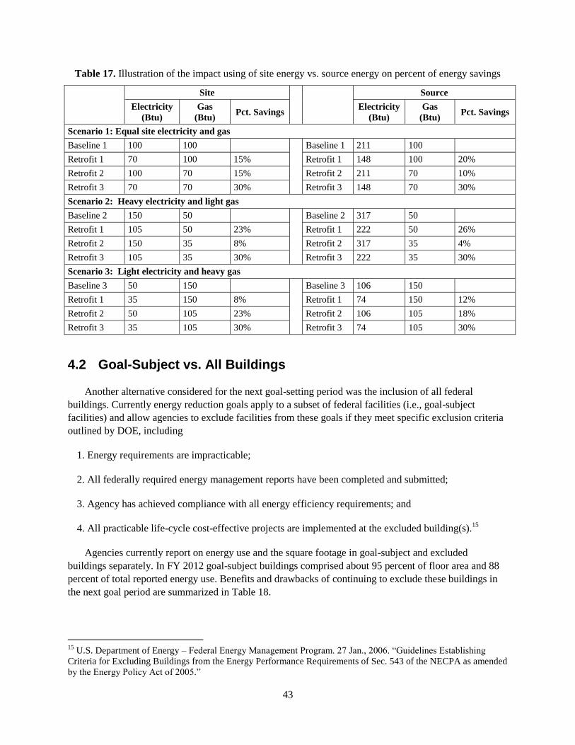
43
Table 17. Illustration of the impact using of site energy vs. source energy on percent of energy savings
Site
Source
Electricity
(Btu)
Gas
(Btu) Pct. Savings
Electricity
(Btu)
Gas
(Btu) Pct. Savings
Scenario 1: Equal site electricity and gas
Baseline 1 100 100
Baseline 1 211 100
Retrofit 1 70 100 15% Retrofit 1 148 100 20%
Retrofit 2 100 70 15% Retrofit 2 211 70 10%
Retrofit 3 70 70 30% Retrofit 3 148 70 30%
Scenario 2: Heavy electricity and light gas
Baseline 2 150 50 Baseline 2 317 50
Retrofit 1 105 50 23% Retrofit 1 222 50 26%
Retrofit 2 150 35 8% Retrofit 2 317 35 4%
Retrofit 3 105 35 30% Retrofit 3 222 35 30%
Scenario 3: Light electricity and heavy gas
Baseline 3 50 150 Baseline 3 106 150
Retrofit 1 35 150 8% Retrofit 1 74 150 12%
Retrofit 2 50 105 23% Retrofit 2 106 105 18%
Retrofit 3 35 105 30% Retrofit 3 74 105 30%
4.2 Goal-Subject vs. All Buildings
Another alternative considered for the next goal-setting period was the inclusion of all federal
buildings. Currently energy reduction goals apply to a subset of federal facilities (i.e., goal-subject
facilities) and allow agencies to exclude facilities from these goals if they meet specific exclusion criteria
outlined by DOE, including
1. Energy requirements are impracticable;
2. All federally required energy management reports have been completed and submitted;
3. Agency has achieved compliance with all energy efficiency requirements; and
4. All practicable life-cycle cost-effective projects are implemented at the excluded building(s).15
Agencies currently report on energy use and the square footage in goal-subject and excluded
buildings separately. In FY 2012 goal-subject buildings comprised about 95 percent of floor area and 88
percent of total reported energy use. Benefits and drawbacks of continuing to exclude these buildings in
the next goal period are summarized in Table 18.
15
U.S. Department of Energy – Federal Energy Management Program. 27 Jan., 2006. “Guidelines Establishing
Criteria for Excluding Buildings from the Energy Performance Requirements of Sec. 543 of the NECPA as amended
by the Energy Policy Act of 2005.”

44
Table 18. Benefits and drawbacks of basing energy reduction goals on goal-subject vs. all buildings
Benefits Drawbacks
Goal-Subject
Buildings Only
• Consistent with current approach
• Focuses on buildings in which energy
may be most effectively managed
(high-energy, mission-critical
exempted)
• Reporting two sets of numbers is more
complicated
• No credit for cost-effective projects
saving energy in excluded facilities
• Process operations within excluded
facilities often present enormous
opportunities for energy savings
relative to the rest of the building
inventory
All Buildings
• Simplifies reporting by establishing
same boundaries as those used for
greenhouse gas (GHG) reporting,
requiring a single energy use number
• Provides more accurate assessment of
actual federal EUI
• Goal-excluded facilities often have
lower energy efficiency reduction
potential
• Certain process loads may still need to
be reported separately
• Does not account for changes in
agency mission requirements that lead
to significant changes in energy use
(e.g. supercomputer deployment)
Maintaining the option to exclude energy intensive buildings from the calculation of EUI would be
consistent with the current reporting approach. This approach may be more favorable to agencies because
many excluded buildings are mission-critical facilities hosting energy-intensive process loads. While
ECMs such as lighting retrofit measures should be implemented in these facilities, the ability to affect
total building EUI may be limited by the magnitude of the process loads. Including these buildings in the
overall calculation may constrain agencies’ ability to meet the energy performance requirement, by
reducing the relative impact of energy efficiency and conservation measures implemented in goal-subject
buildings on overall energy use. At the same time, the current approach does not award agencies credit for
energy-saving measures that are taken in excluded buildings, which have led to sizeable savings in some
buildings.
Eliminating the exclusion of certain facilities from the EUI performance goals would simplify the
reporting process, as agencies would only need to provide a single set of energy use numbers by eGRID
subregion. Eliminating the exclusion would more closely align energy performance reporting
requirements with GHG reporting requirements, which does not distinguish between goal-subject and
goal-excluded facilities. However, these may not align perfectly as certain structures and processes not
qualified as federal buildings that are covered by GHG reporting would still be exempt from energy
performance (e.g. federal ships that consume “Cold Iron Energy”, which supplies power and heat to ships
docked in port). It would also provide a more accurate assessment of actual federal energy intensity.
To illustrate the impact of including goal-subject buildings in the EUI reduction goals, the energy use
and associated building square footage of excluded buildings was added back into the federal building
inventory (Figure 24).

45
Figure 24. Reduction in site EUI for goal-subject buildings and all buildings, FY 2008-2012
The analysis of the impact of future retrofit measures on overall EUI was based on total floor area in
the federal sector. The modeling approach did not allow for separate model runs in goal-subject and goal-
excluded buildings. Similarly, no distinction between goal-subject and goal-excluded buildings was made
for the impact of new buildings, as there is no reliable basis for establishing prototypes that would
exclude floor area not subject to efficiency goals. Any impact would be negligible, as the overall
percentage of new building floor space that might be excluded under current high-intensity criteria would
likely be less than one percent of the total 2025 stock.
4.3 FY 2003 vs. Alternative Baseline Years
A number of criteria should be considered when establishing the baseline year for the next federal
energy reduction goal. Weather is one of the most important considerations when establishing a baseline
year for energy performance goals, but other factors, including data quality and availability, consistency
with other baseline year requirements, agency mission tempo, public perception around savings, and the
diverse starting points of agencies should also be considered.
This section evaluates the advantages and disadvantages of maintaining the current baseline year of
FY 2003 versus using alternative years for the 2025 energy reduction goal. Alternative years evaluated
included FY 2008 (for consistency with greenhouse gas reporting) and either FY 2013 or FY 2015 to
represent current baseline performance at the beginning of the goal period. Yet another alternative is to
use a three-year average baseline to normalize for some of the factors described above.
4.3.1 Weather
Ideally the baseline year would represent a fairly typical weather year in terms of the demand for
heating and cooling of buildings. A simplistic analysis of heating degree days (HDD) and cooling degree

46
days (CDD) days in recent fiscal years provides some insight into how typical or anomalous different
fiscal years have been and therefore which may provide an appropriate baseline year for a 2025 reduction
target. The research team examined HDD and CDD data for 12 geographic locations with a significant
portion of the federal building stock and compared those to historical averages over a 14-year period
between FY 2000 and FY 2013. Data were derived using a simple online weather station reporting tool
from EnergyCAP, Inc., (www.weatherdatadepot.com) (Table 19). Conditional formatting was used to
illustrate outlier years of either warmer- or colder-than-normal weather, based on degree days. Thus, the
lighter the shades of coloring, the closer to the period average that year was for the specific location. To
identify the best weather-neutral year across the wide geography of the United States, we would select a
year that is reasonably lightly shaded at the USA (sum) line for both HDD and CDD.
The current baseline year of FY 2003 appears to be one of the colder years of the period examined
(implying higher than average heating loads, and lower than average cooling loads). Visual inspection
suggests either FY 2008 or FY 2013 as the most weather-neutral year, despite some geographic variation
in those years. Alternatively, FY 2004 appears to be closest to the period average for HDD, while FY
2008 appears to be closest to the period average for CDD.
Table 19. Total heating degree days and cooling degree days for 12 U.S. cities
Heating Degree Day Summary (FY Basis and 65°F Basis)
Year 2000 2001 2002 2003 2004 2005 2006 2007 2008 2009 2010 2011 2012 2013
Atlanta 2413 3062 2363 2863 2657 2527 2638 2444 2530 2713 3203 2790 1977 2517
Chicago 5047 6068 5239 6373 5964 5712 5767 5945 6263 6419 5768 6424 4939 6163
Dallas 1541 2647 2063 2303 1861 1762 1606 2064 1966 1898 2470 2003 1823 1819
DC 3630 4315 3300 4565 4026 4021 3710 3954 3454 4216 3828 4002 3119 3759
Denver 5237 6359 5988 6100 5735 5780 5566 6074 6123 5619 6337 5796 5599 6014
Houston 835 1554 1124 1344 1085 953 923 1180 932 1000 1621 1126 891 972
LA 941 1335 1060 923 1002 1052 1090 764 1148 826 822 1134 1404 949
Memphis 2486 3411 2675 3164 2803 2405 2658 2765 2750 2967 3244 2945 2226 2929
New York 4479 4954 3853 5301 4800 4707 4287 4458 4466 4843 4343 4750 3818 4614
Phoenix 803 1175 871 664 903 861 745 949 958 708 914 893 968 881
Seattle 4783 5073 5021 4458 4474 4452 4400 4752 5152 4867 4642 4999 4941 4191
St. Louis 4056 5246 4145 4947 4333 4230 4297 4423 4823 4767 4874 4912 3563 4658
USA (sum) 36251 45199 37702 43005 39643 38462 37687 39772 40565 40843 42066 41774 35268 39466
Cooling Degree Day Summary (FY Basis and 65°F Basis)
Year 2000 2001 2002 2003 2004 2005 2006 2007 2008 2009 2010 2011 2012 2013
Atlanta 1870 1691 1989 1664 1811 1835 2048 2225 1949 1895 2382 2242 2074 1727
Chicago 1017 974 1260 700 687 1197 936 997 873 587 1132 1001 1269 816
Dallas 3255 2983 2907 2838 2819 3276 3563 2846 3128 2981 3223 3741 3275 3334
DC 1228 1401 1844 1338 1565 1666 1545 1702 1815 1461 2095 1913 1864 1679
Denver 962 974 917 758 511 913 961 975 828 533 862 871 1119 997
Houston 3451 3122 3176 3092 3182 3534 3349 3328 3575 3482 3316 3851 3398 3356
LA 1335 981 974 1166 1388 950 1590 1376 1447 1565 1206 980 992 1310
Memphis 2468 2366 2329 1938 2148 2600 2532 2784 2342 2154 2753 2538 2611 2191
New York 899 1195 1386 1031 1061 1440 1150 1139 1248 876 1541 1273 1193 1240
Phoenix 4973 4793 5139 4791 4977 4554 4824 5091 4845 5010 4589 4884 4824 5186
Seattle 109 72 162 273 273 162 270 192 193 314 162 100 154 385
St. Louis 1345 1510 1667 1273 1144 1555 1474 1711 1301 1204 1570 1603 1802 1368
USA (sum) 22912 22062 23750 20862 21566 23682 24242 24366 23544 22062 24831 24997 24575 23589
Warmer than average
Colder than average
47
4.3.2 Other Factors
Factors other than weather that might influence baseline year selection include
Data quality – The quality of energy use and building area data reported should be considered.
As metering of facilities and reporting have become more commonplace across the federal sector,
driven in part by the EPAct 2005 advanced metering requirements, data quality has improved.
While there may be site-specific exceptions, more recent baseline years are believed to be much
more accurate for this reason. This suggests that FY 2013, which was also a typical weather year,
may be a very good option. Alternatively, establishing a future year as the baseline year at the
beginning of the goal period (2015) would give agencies an opportunity for advance preparation
for data collection and potential adjustments for mission tempo and other factors.
Consistency with other baseline years – Currently agencies have an FY 2003 baseline for EUI
reduction goals and a FY 2008 baseline for facility greenhouse gas reduction goals. Both the EUI
and greenhouse gas goals rely on the same data inputs. Tracking progress could be simplified if
the baseline years for both goals were aligned and FY 2008 was used moving forward.
Mission tempo – Mission tempo, or the rate of operations relative to a typical year for the
agency, can have a big impact on energy use, particularly for the DOD. Mission tempo will vary
across agencies year to year, and it is unlikely that a single year will be typical for all agencies.
While FY 2003, FY 2008, and FY 2013 do not appear to be anomalous in terms of unusual spikes
in agency energy use reporting, agencies should be consulted on these options to verify that
assumption.
Perceived savings – The baseline year selected will influence the percent reduction in EUI that is
feasible. Maintaining the current FY 2003 baseline year would result in an additive goal; for
example, the current 30 percent through 2015 plus another 20 percent of savings from 2015-2025
results in a total goal of 50 percent. This would convey the cumulative progress made by the
federal government over two decades. Using a more recent baseline year—and a setting a lower
percent reduction goal—may give the impression that the federal government is not doing enough
to reduce energy use, when in fact significant reductions have already been made.
Accounting for diverse starting points – Individual agencies have shown a wide range of
progress toward the EUI reduction goals between 2003 and 2012, from a modest 3 percent up to
45 percent savings. The amount of future savings potential ultimately depends on the starting
point of each agency, including the nature of their buildings, operations, and types of ECMs that
have already been implemented. Maintaining the current baseline year of FY 2003 would allow
agencies that have done more already to do less in the future, as they likely have lower savings
potential. Those agencies would not be penalized for having already made substantial reductions.
In contrast, agencies that have fallen well short of the 30 percent goal to date would be expected
to catch up by FY 2025. If a more recent goal year were used, such as FY 2013, agencies would
be starting with a clean slate.
Availability of electricity data by region – Federal agencies did not begin reporting electricity
data by eGRID subregion until FY 2008, when it was required to support greenhouse gas

48
reporting. If the federal government were to move toward a fossil-source energy accounting
approach based on regional factors, the only feasible baseline years would be FY 2008 and after.
Table 20 summarizes these variables and the baseline years considered, and provides a simplistic
evaluation of how each year rates against the criteria discussed above. For example, FY 2013 and FY
2008 appear to be good potential baseline years considering the impacts of weather on energy use,
whereas the current FY 2003 baseline year was not a typical weather year. A limitation of using FY 2015
is that weather and other factors that may influence energy performance are unknown at this point.
Table 20. Possible baseline years and an evaluation of how each year rates against different criteria;
green is a comparatively good year, yellow is neutral, and red is comparatively bad
Baseline Year Selection Factor FY 2003 FY 2008 FY 2013 FY 2015
Weather unknown
Data quality likely
Consistency with other baseline years unknown unknown
Mission tempo unknown
Perceived savings
Account for diverse starting points
Availability of electricity data by region
4.4 Single vs. Distinct or Tiered Performance Goals
Currently, all federal agencies are working toward a single EUI reduction goal. An alternative
approach is to establish unique targets based on each agency’s future savings potential, or two to three
tiers of targets (e.g. 30%, 20%, and 10%) that would apply to different agencies. Establishing a single
goal for all agencies is the simplest approach and would facilitate tracking. A single federal goal has been
established for almost all federal energy requirements with the exception of the greenhouse gas emissions
management, which allowed each agency to evaluate their reduction potential and negotiate a goal with
the Offices of the White House.
Setting agency-specific or tiered goals would provide an opportunity to better align goals with each
agency’s potential to reduce energy. Agencies that have already made substantial EUI reductions would
not be penalized by having to achieve a goal that is beyond their potential, and agencies that have lagged
on progress would be pushed to do more. Rather than setting a conservative goal that works for all
agencies, unique goals that are based on each agency’s true potential may allow for greater government-
wide savings. For this approach to be effective, however, goals must be based on well-informed estimates
of savings potential. These might be based on a combination of prior EUI reduction performance, current
EUIs, and modeled estimated of future savings potential.
The analysis of savings achieved by each major agency to date illustrates that agencies have achieved
a wide range of savings since the FY 2003 baseline. These EUI reductions from 2003-2012 range from 3
percent to 45 percent as illustrated in Table 3. However, only five scorecard agencies appear to be
significantly lagging; most are on track to achieving their goals with savings in the 20 to 30 percent range.

49
This suggests that with the exception of a few high and low outliers, most agencies are reducing building
EUI at a similar rate. Analysis of the average EUIs by agency also shows a wide performance range from
50,000 kBtu/SF to 300,000 kBtu/SF (see Figure 4), and about eight agencies with extremely high average
EUIs. Agencies with both high EUIs and limited EUI reduction progress may be candidates for higher
EUI reduction goals and vice-versa.
The forward-looking analyses of potential savings from existing building retrofits and new
construction examined the potential savings from civilian agencies and the DOD separately to account for
significant differences in utilization and performance of those facilities, but did not examine the savings
potential of each agency. Further disaggregation by agency would have required several additional model
runs and specific assumptions for each agency, and was beyond the scope of this effort.
4.5 Intensity vs. Absolute Reduction Goals
The benefits and drawbacks of using of an absolute energy (Btu) reduction target rather than an
energy-intensity target are summarized in Table 21.
Currently Btu per square foot is used as the intensity metric and remains the most practical
normalizing metric in light of data federal reporting and availability. However the limitations of this
intensity Btu/SF metric to normalize energy performance should be considered. While private entities
may normalize energy use using business metrics (e.g. energy use per million $ of sales), such metrics are
not practical for the federal sector. Furthermore, average occupant density, computer density, and other
factors can also have a significant influence on building performance. In the case of occupant density,
increased occupant density can be environmentally beneficial if it reduces the need for additional building
area.
Table 21. Benefits and drawbacks of setting energy intensity vs. absolute reduction goals
Benefits Drawbacks
Energy Intensity
(Btu/SF) Reduction
Goals
• Reflects performance
improvements independent of
increases and decreases in floor
area
• Enables performance comparison
across agencies
• No guarantee that total energy
consumption (and environmental impact)
is reduced, even if intensity decreases
• If normalization is the intent, EUI only
partially normalizes energy use, as
factors other than floor area can have a
significant influence on performance (e.g.
occupant density)
Absolute Energy
Reduction Goals
• Environmental impact of
reduction measures is easier to
ascertain
• Energy savings are more
transparent to stakeholders
• Evolving mission requirements may lead
to increases in energy demand that cannot
be managed
• Accurate targets require more accurate
baseline year characterization by agency
• Does not allow for direct performance
comparison of efficiency improvement
across agencies

50
While not a tradeoff of selecting an intensity versus absolute target, an additional consideration may
be that the current GHG emissions reduction goal required under Executive Order 13514 is an absolute
reduction goal and currently includes all aspects of facility energy use, as well as non-building fuel uses.
An absolute facility energy goal would be in some respects redundant with the absolute GHG reduction
target. On the other hand, an absolute energy reduction goal codified under law out to 2025 would have a
longer term impact than the current 2020 GHG reduction goal.
4.6 Other Goal-Setting Approaches
Several other goal-setting approaches were considered as part of this study but were not evaluated in
detail due to current data constraints. These may be revisited in the future as federal building performance
data quality improves.
Set EUI reduction targets by building type and location – This approach would account
for the current building performance and unique building stock characteristics of each federal
agency, and therefore result in more realistic reduction targets by agency. Building type and
location both have a significant influence on energy performance and the types of ECMs that
are appropriate. Under this scenario, each agency would have different overall energy
reduction potential based on the current efficiency and characteristics of its building
inventory. The building type disaggregation presented in Table 4 of this study could inform
such an approach for the civilian sector, but a more robust analysis of both DOD and civilian
buildings would be required for target-setting. This was beyond the scope and resources
available for this study. If EUI targets are to be set by building type and location, it is
recommended that they are based on actual federal audit results from a cross-section of
common federal building types and locations/climate zones across multiple federal agencies.
Modeling of federal agency specific data would be much more labor intensive but estimates
of building energy performance would be more accurate. This type of analysis may be more
feasible as a larger portion of the federal building stock is entered into Energy Star Portfolio
Manager.
Require Energy Star score of 75 or higher for some percent of the agency’s buildings –
This approach would be useful if the objective were ensuring that federal building were high-
performing compared to the general building stock and enabling normalization to account for
the many variables other than square footage that influence building performance. For
example, occupancy, computers density, operating hours, space conditioning and location-
specific climate impacts on energy use are all accounted for when arriving at a normalized
Energy Star score. The primary drawback of this approach is that there is a significant
reporting burden. While it is already a federal requirement to enter metered buildings into
Energy Star Portfolio Manager (which will generate a performance score), only a small
percentage of all federal buildings are currently entered into Portfolio Manager.
Set energy cost reduction targets – If cost savings are the primary driver, energy cost
reduction targets could be established. The risk of this approach is that rising utility rates and
variability of utility rates by region could result in investments that are uneven geographically
as an unintended consequence, leaving many buildings under-performing.
51
5.0 Conclusions and Recommendations
This study aims to inform policymakers in setting future energy reduction goals by establishing past
performance toward the current energy intensity reduction goal and future energy savings potential from a
combination of retrofits to existing federal buildings and the addition of newly constructed facilities to the
federal building stock. It also evaluates the benefits and drawbacks of alternative goal-setting approaches
and baseline years.
When setting future energy reduction goals, policymakers should consider that factors other than past
EUI reduction performance and estimated savings from future investments in cost-effective energy
conservation measures will also influence what targets are feasible, and furthermore that there is always
uncertainty in projecting the future. Budgetary constraints, operational preferences, and organizational
limitations, such as mission requirements for energy security or availability of staffing for ongoing O&M
of new technologies, will all influence what is practical and feasible to implement. Anticipating these
factors was outside the scope of this study, however cost estimates were provided in section 3.1.5 to
illustrate general levels of funding that would be required to achieve these EUI values. As a result, it
should be emphasized that the EUI reduction estimates presented in this study represent key inputs to the
goal-setting process but not actual reduction goals.
The analysis of past performance suggests that the federal government as a whole is on track to just
meet the 30 percent reduction target by 2015. As of FY 2012, the federal government reported a 21
percent decrease from the FY 2003 baseline with 18 of 24 OMB scorecard agencies achieving at least a
21 percent reduction in energy intensity, which is the OMB target for “on track”. DOD alone is
responsible for about 60 percent of all federal energy use and building area, so its performance will
significantly influence whether the federal government achieves a 30 percent reduction in energy intensity
target.
This past EUI reduction was driven by an 18 percent decrease in site-delivered energy use and a 3
percent increase in goal-subject floor space. While electricity represents the largest source of site-
delivered energy use in the federal government, at 50 percent, the majority of federal energy savings came
from primary fossil sources. The largest absolute reductions came from fuel oil and natural gas savings,
which each represented 31 percent of total energy savings; in comparison, 17 percent of savings were
from electricity. The majority energy saved by DOD was from fuel oil, natural gas, and coal sources.
ECMs in the USPS contributed to half of the total electricity savings, while DOE contributed 34 percent
of government-wide electricity savings.
Modeled estimates of future savings potential from the implementation of lifecycle cost-effective
ECMs in existing buildings suggest that civilian agencies could reduce energy intensity by 11 percent
between 2015 and 2025, while DOD could reduce its energy intensity by 22 percent. The combined total
estimated savings potential from retrofits in all federal buildings is 20 percent from 2015-2025. The
greatest savings opportunities in civilian agency buildings come from lighting ECMs. In DOD, envelope
improvements, such as adding insulation in roofs and walls, are expected to contribute the most to
savings. By building type, the greatest savings in the civilian sector are expected to come from ECMs
implemented in office buildings.

52
The federal inventory will also experience some turnover between 2016 and 2025, as old buildings
are retired and new buildings are constructed. These new federal buildings will be subject to more
stringent design standards aimed at improving their energy performance. This is expected to support
another 2.7 percent reduction in all federal facilities, with 1.5 percent in the military sector and 4.5
percent in the civilian sector. The comparatively larger impact on the civilian sector is due to projections
that DOD will be turning over less floor area in the next decade —perhaps due to a recent spike in DOD
construction— compared to projected turnover in the civilian building stock.
The combined impact of implementing cost-effective retrofit measures and new construction is
presented in Table 22 below.
Table 22. Estimated EUI impact from both cost-effective retrofits to existing buildings and federal
energy standards for new construction (site energy basis)
Building Type
Existing Buildings New
Buildings Total Stock
2015
EUI
2025 EUI
Reduction
(Efficiency Only)
2025
EUI
2025 EUI
Reduction 2025 EUI
kBtu/SF kBtu/SF Pct. kBtu /SF kBtu/SF kBtu/SF Pct.
Change
All Civilian 97.3 10.9 11.2% 86.3 4.3 82.0 15.7%
Civ: Health Care 151.9 15.9 10.5% 135.9
Civ: Industrial 98.7 10.5 10.6% 88.2
Civ: Laboratory 145.0 13.6 9.4% 131.5
Civ: Office 92.0 10.6 11.5% 81.4
Civ: Prison 129.1 13.5 10.5% 115.5
Civ: School 73.8 9.2 12.5% 64.6
Civ: Service 68.3 8.8 12.8% 59.5
Civ: Warehouse 27.1 5.6 20.7% 21.5
Civ: Other 84.1 10.0 11.9% 74.1
DOD 91.0 20.4 22.5% 70.6 1.4 69.2 24.0%
Total Federal 93.1 18.5 19.9% 74.5 2.5 72.0 22.6%
The addition of onsite renewable energy could support up to another 4 percent reduction in site-
delivered energy intensity in civilian agencies and an additional 9 percent for the DOD. It should be
noted, however, that renewable energy savings are based on technical feasibility and do not reflect
lifecycle cost-effectiveness, which would require additional information on state policies and incentives
and site-level characteristics. As a result, it is recommended that the renewable savings estimates might
be considered an upper limit for goal-setting purposes considering the lower level of certainty around
these estimates.
Based on the information available for the modeling and analysis included in this report, the larger
energy-savings potential in DOD facilities compared to the civilian sector may be attributed to the age of
the DOD building stock and the progress toward the EUI reduction goal to date. The DOD stock is older
and was not, until the last decade or so, built to the same standards. For example, uninsulated metal-sided
and metal-roofed buildings constructed for unoccupied and unconditioned storage have been repurposed
to heated, occupied warehousing. Such examples may explain in part the lower starting EUIs and
challenge associated with reducing them further. The nature of the DOD stock also results in significant
53
retrofit opportunities for envelope measures that increase insulation and reduce heating and cooling loads.
Further, the DOD sector has achieved a 17.7 percent reduction from its 2003 baseline, while the civilian
sector has reduced energy use intensity 24.5 percent below its baseline. One reason for the higher civilian
EUI reductions may be that the civilian sector as a whole has invested comparatively more into building
efficiency than DOD during the goal period. Finally, the fact that DOD space has become more highly
utilized in recent years may also be influencing DOD slower EUI reduction rates.
The total estimated investment required to achieve these savings through energy efficiency retrofits
only (excludes renewable energy) is $8.3 billion, approximately $5.0 billion of which would be required
to fund DOD retrofits. This would equate to an annual investment in retrofits of roughly $830 million
over the ten-year goal period. The estimated annual savings from the combined cost-effective measures
totals $1.2 billion per year, $700 million of which would come from DOD investments in ECMs and $520
million per year would come from civilian sector investments. This suggests that all cost-effective ECMs
in federal buildings would produce a simple payback of around seven years, assuming funding through
direct appropriations. It should be considered that some portion will likely be funded through third-party
mechanisms, such as ESPCs, although this will vary by agency. Due to different payback thresholds and
higher financing costs, some of the long-payback items that are cost-effective with direct appropriations,
may not occur under a third-party financing scenario, therefore the total investment and savings potential
would be somewhat lower.
Defining the optimal goal-setting approach ultimately depends on what policymakers and the
government seeks to accomplish through energy management. Several approaches to establishing goals
and baseline years for the 2015 to 2025 goal-period were considered, including using site versus source
energy factors, removing the exclusion of certain energy-intensive buildings, setting agency-or sector-
specific goals versus a single federal sector goal, and establishing alternative baseline years. Based on the
analysis of the benefits and drawbacks of each of these approaches, the following recommendations are
made:
Fossil-source energy, using national eGRID factors, should provide the basis for 2025 goals
that better reflect total energy use impacts and savings. The impact on savings by agency is
expected to be nominal overall.
All buildings should be subject to goals, to simplify reporting and provide opportunities for
additional savings in these buildings, assuming that process operating loads not attributed to a
building function (e.g. docked ships) can be reported separately.
Separate goals should be established for DOD and the civilian sector to account for the
different savings potential in each sector.
A tiered approach should be established with three levels of goals, to account for variability
in civilian sector EUIs and EUI reduction potential.
A new baseline year should be established that is closer to the beginning of the goal period.
Fiscal year 2013 represents a good weather year and is close to the basis used for modeled
results. Furthermore, data quality is probably better than previous years considering the
recent push to increase building-level metering quality.

54
6.0 References
111 USC Sec. 405. 2009. The American Recovery and Reinvestment Act of 2009. Public Law 111-5.
Available at http://www.gpo.gov/fdsys/pkg/BILLS-111hr1enr/pdf/BILLS-111hr1enr.pdf. (undated
webpage).
American Society of Heating, Refrigerating and Air-Conditioning Engineers (ASHRAE) and Illuminating
Engineering Society of North America (IESNA). 1975. Energy Conservation in New Building
Design. ASHRAE Standard 90-75, Atlanta, Georgia.
American Society of Heating, Refrigerating, and Air-Conditioning Engineers (ASHRAE) and
Illuminating Engineering Society of North America (IESNA). 1980. Energy Conservation in New
Building Design, ANSI/ASHRAE/IES 90A-1980, New York.
American Society of Heating, Refrigerating, and Air-Conditioning Engineers (ASHRAE) and
Illuminating Engineering Society of North America (IESNA). 1990. Energy Efficient Design of New
Buildings Except Low-Rise Residential Buildings, ANSI/ASHRAE/IES 90.1-1989, Atlanta, Georgia.
American Society of Heating, Refrigerating, and Air-Conditioning Engineers (ASHRAE) and
Illuminating Engineering Society of North America (IESNA). 2004. Energy Standard for Buildings
Except Low-Rise Residential Buildings. ANSI/ASHRAE/IESNA Standard 90.1-2004, Atlanta, Georgia.
American Society of Heating, Refrigerating, and Air-Conditioning Engineers (ASHRAE) and
Illuminating Engineering Society of North America (IESNA). 2007. Energy Standard for Buildings
Except Low-Rise Residential Buildings. ANSI/ASHRAE/IESNA Standard 90.1-2007, Atlanta, Georgia.
American Society of Heating, Refrigerating, and Air-Conditioning Engineers (ASHRAE) and
Illuminating Engineering Society of North America (IESNA). 2010. Energy Standard for Buildings
Except Low-Rise Residential Buildings. ANSI/ASHRAE/IESNA Standard 90.1-2010, Atlanta, Georgia
EISA 2007 – Energy Independence and Security Act of 2007. 42 USC 17001. Public Law No. 110-140.
EPAct – Energy Policy Act of 2005. 2005. 42 USC 15801 et seq. Public Law No. 109-58, as amended.
Judd KS, AR Kora, JW Henderson, BJ Russo, J Katz, M Hummon, and EM Rauch. 2010. Roadmap to a
Climate Neutral Federal Government. PNNL-19643, Pacific Northwest National Laboratory, Richland,
WA.
NECPA – National Energy Conservation Policy Act. 42 USC 8251. Public Law 95–619.
Rushing, AS, JD Kneifel, BC Lippiatt. 2013. Energy Price Indices and Discount Factors for Life-Cycle
Cost Analysis - April 2010: Annual Supplement to NIST Handbook 135 and NBS Special Publication
709. NIST Interagency/Internal Report (NISTIR) - 85-3273-25.
Thornton BA et al. 2011. Achieving the 30% Goal: Energy and Cost Savings Analysis of ASHRAE
Standard 90.1-2010. PNNL-20407, Richland, WA.

55
U.S. Department of Energy. 2011. U.S. Department of Energy Commercial Reference Building Models
of the National Building Stock.

A-1
Appendix A. Methodology for Estimating Existing Building
Retrofits
The prototype buildings were modeled using the 2013 release of the Facility Energy Decision System
(FEDS) – a tool for simulating building energy performance and analyzing the impact of energy
conservation measures (ECMs). The FEDS inference engine uses building type, location, size, and
vintage to statistically infer technology retirement and estimate what technologies still exist in the
building stock and their performance.
The intent of the FEDS model is to provide information needed to determine the minimum life-cycle
cost (LCC) configuration of the energy generation and consumption infrastructure for both federal
civilian buildings and integrated military installations. The model has no fuel or technology bias; it
selects the technologies that will provide an equivalent or superior level of service (e.g., heating, cooling,
illumination) at the minimum LCC.
The FEDS models use the FEMP-prescribed (NIST 2013) utility escalation rates for gas and
electricity. Discount rates and calculation methodologies used in the analysis also follow guidelines
established in NIST guidance: http://www1.eere.energy.gov/femp/pdfs/ashb13.pdf.
As part of estimating the minimum LCC configuration of generation and end-use technologies, all
interactive effects between energy systems are explicitly modeled. The value or cost of these interactive
effects varies by building type (level of internal gain), building size (portion of heating, ventilation, and
air conditioning loads attributable to internal gains versus envelope gains/losses), climate (whether a
particular building is cooling- or heating-dominated), occupancy schedule, and a number of other factors.
Thus, there is no simple solution, and detailed simulation modeling is the best way to provide a credible
estimate of the impact. For example, when considering a lighting retrofit, the model evaluates the change
in energy consumption in all building energy systems rather than just the change in the lighting energy.
The analyses yielded a life-cycle-cost-effective mix of energy conservation measures, which resulted
in Energy Use Intensities (EUIs) for each of the prototype buildings and locations. The specific analysis
assumptions are described below.
A.1 Selecting Building Types and Locations to Model
A.1.1 Civilian Buildings
Prototype buildings modeled for the civilian stock, and their basic operating characteristics, are
summarized in Table A.1. Each variant was weighted based on region and proportion of the stock. All
simulations were based on 2011 prototype buildings and starting EUI values were adjusted to 2015 based
on perpetuating current goal compliance trends over the 2011-2015 period. (See Section 3.1.2 of the
report.)
Prototype buildings were constructed for simulation in FEDS based on statistical analysis of stock
average characteristics including floor area, vintage, size, operating schedules, and predominant heating,
ventilating and air conditioning (HVAC) system types. More details on baseline heating and cooling
technologies can be found in Section A.2.

A-2
Table A.1. Characteristics of civilian sector buildings modeled in FEDS and operation assumptions
Building Type Vintage Size (SF) Operation Hours Ventilation
Healthcare 1994 200,000 24/7 Constant operation
Healthcare 1994 30,000 6:00am to 6:00pm Mon-Fri
11:00am to 1:00pm Sat-Sun
Constant operation
Healthcare 1957 200,000 24/7 Constant operation
Healthcare 1957 30,000 6:00am to 6:00pm Mon-Fri
11:00am to 1:00pm Sat-Sun
Constant operation
Laboratory 1994 200,000 7:00am-6:00pm Mon-Fri
Constant during occupied hours,
cycle during unoccupied hours
Laboratory 1994 30,000 7:00am-6:00pm Mon-Fri
Constant during occupied hours,
cycle during unoccupied hours
Laboratory 1957 200,000 7:00am-6:00pm Mon-Fri
Constant during occupied hours,
cycle during unoccupied hours
Laboratory 1957 30,000 7:00am-6:00pm Mon-Fri
Constant during occupied hours,
cycle during unoccupied hours
Office 1994 340,000 7:00am-6:00pm Mon-Fri Constant operation
Office 1994 90,000 7:00am-6:00pm Mon-Fri
7:00am-6:00pm Mon-Fri
Constant during occupied hours,
cycle during unoccupied hours
Office 1994 5,000 7:00am-6:00pm Mon-Fri
Constant during occupied hours,
cycle during unoccupied hours
Office 1957 340,000 7:00am-6:00pm Mon-Fri Constant operation
Office 1957 90,000 7:00am-6:00pm Mon-Fri
7:00am-6:00pm Mon-Fri
Constant during occupied hours,
cycle during unoccupied hours
Office 1957 5,000 7:00am-6:00pm Mon-Fri
Constant during occupied hours,
cycle during unoccupied hours
Warehouse 1994 200,000 7:00am-5:00pm Mon-Fri
11:00am-2:00p Sat
11:00am-1:00pm Sun
Cycle with cooling and linked
heating systems
Warehouse 1994 30,000 7:00am-5:00pm Mon-Fri
11:00am-2:00p Sat
11:00am-1:00pm Sun
Cycle with cooling and linked
heating systems
Warehouse 1957 200,000 7:00am-5:00pm Mon-Fri
11:00am-2:00p Sat
11:00am-1:00pm Sun
Cycle with cooling and linked
heating systems
Warehouse 1957 30,000 7:00am-5:00pm Mon-Fri
11:00am-2:00p Sat
11:00am-1:00pm Sun
Cycle with cooling and linked
heating systems
The set of 30 prototypes in Table A.1 as modeled for each region using the applicable TMY weather
data for a representative city in the region (Table A.2).
Table A.2. Region specifications for civilian stock
Region TMY City
CA Los Angeles, CA
DC/MD/VA Washington, DC
FL/GA Jacksonville, FL
NY New York, NY
TX Dallas, TX

A-3
In some cases, multiple prototypes were simulated to capture variation in the stock. For example, the
office type represents a very large fraction of the civilian building stock. To better represent offices, the
population of buildings was split into three size categories, rather than the two size categories used for the
other building types. Additionally, some building types represent a very diverse collection of buildings,
and as such, the buildings within the type have a large variety of HVAC systems. The research team
selected the predominant HVAC system types within each building type and modeled them as separate
prototypes.
FEDS performs retrofit simulations based on an extensive and continuously updated library of ECMs.
For each building prototype simulated, FEDS identifies the package of ECMs that minimizes total LCC,
given the prototype’s end-use load profile, current mix of technologies, baseline expenditures for
electricity, gas and all other fuels, electricity and gas rate structures, and applicable demand charges.
ECMs include the potential for technically achievable onsite renewable technologies to be employed
to contribute to EUI reductions. For civilian buildings, solar photovoltaic (PV) systems were sized for the
prototype buildings such that system production would not exceed the electric energy demand of the
building in any concurrent hour. This constraint prevents consideration of cases where onsite renewables
could supply power back to the grid – distorting the impact on the buildings’ EUI. Additionally, the size
of the PV array was constrained to be no greater than that which would fit on the roof of the modeled
building.
In addition to ECMs and onsite renewables modeled in FEDS, the research team conservatively
assumed that civilian buildings could achieve an additional 5 percent savings through improved
operations and continuous commissioning activities at a cost equivalent of a three-year simple payback.
A.1.2 DOD Buildings
In determining the optimal retrofit for each technology within the military sector, the interactions at
the installation level are considered by determining the impact on the installation's electric energy and
demand cost, as well as the interactive effects among end-uses. This is important because the peak
electric demand in any individual building may not occur at the same time as the installation's peak
demand. Since the buildings on large federal installations typically are not individually metered, the
installation is billed based on the combined demand of all buildings. Thus, proper valuation of the
changes in an individual building's electric demand must be done in the context of the impact on the
installation's demand profile—including time-of-day pricing and demand ratchets.
For DOD locations, alternative configurations of wind and PV were modeled under the same
constraint as the civilian buildings with the exception of the rooftop requirement as it was assumed that
DOD installations have sufficient land area that roof-mounted PV is not a requirement. Systems were
sized such that renewable output would not exceed aggregate building energy demand in any hour and
were evaluated in alternative configurations such as 25% wind/75% PV, 75% wind/25% PV, 50%
wind/50% PV, 100% wind/0% PV, and 0% wind/100% PV, to select the renewable annual output-
maximizing alternative.
As with civilian buildings, the research team conservatively assumed that DOD installations could
achieve an additional 5 percent savings through improved operations and continuous commissioning
activities, beyond the modeled savings from ECMs and renewables. These activities reduce any savings

A-4
degradation that occurs without regular maintenance and help avoid the emergence of new system
inefficiencies.
Five locations similar to those chosen for the civilian stock were chosen to be regionally
representative of DOD’s footprint. Table A.3 indicates the specific facilities and weather locations for
each installation modeled.
Table A.3. Region specifications for DOD stock
Region Installation TMY Location
CA Fort Hood16
Edwards Air Force Base, CA
DC/MD/VA Fort Belvoir Richmond, VA
FL/GA Fort Benning Jacksonville, FL
NY Fort Drum Watertown, NY
TX Fort Hood Dallas, TX
A.2 Baseline Building Assumptions
The tables that follow highlight some of the key baseline conditions of the modeled buildings in the
civilian and DOD sectors, as well as the general types of retrofit opportunities that were applied.
16
Because PNNL did not have an installation modeled in California, Edwards Air Force Base was used for weather
data and a California rate structure was applied to that site, however the buildings and technologies modeled were
based on Fort Hood.

A-5
Table A.4. Key civilian sector model inputs: office space
Office - Small/New Office - Small/Old Office - Medium/New Office - Medium/Old
Baseline Retrofit Baseline Retrofit
Lighting17 Lighting Lighting Lighting
CFL No change CFL No change CFL No change CFL No change
INC CFL INC CFL INC CFL INC CFL
FL: T12, T8* FL: Super T8 or
No change FL: T12, T8*
FL: Super T8 or
No change FL: T12, T8*
FL: Super T8 or No
change FL: T12, T8*
FL: Super T8 or
No change
HPS No change HPS No change HPS No change HS No change
MH MH or No change MH MH or No change MH MH or No change MH MH or No change
Exit: INC or LED
Exit: Self
Luminous
Electroluminescent
No change
Exit: INC or LED
Exit: Self
Luminous
Electroluminescent
No change
Exit: INC or LED
Exit: Self
Luminous
Electroluminescent
No change
Exit: INC or LED
Exit: Self
Luminous
Electroluminescent
No change
Hot Water Hot Water Hot Water Hot Water
Electric water
heater
No change Electric water
heater
Aerators, Lower
Tank Temperature
(All), Insulate
Tank (CA, NY),
Insulate Pipe (FL,
DC)
Nat Gas Central
Boiler
Conventional Gas
Boiler - 84%
Combustion
Efficiency (TX, NY,
DC), Central Heat
Pump Hot Water
System (CA), Wrap
Tank (All)
75% Nat Gas
Central Boiler
25% Electric
Water Heater
Conventional Gas
Boiler - 84%
Combustion
Efficiency (TX,
NY, CA, FL) or
Central Heat Pump
Hot Water System
(DC), Wrap tank,
Aerators (All)
Aerators, Lower
Tank Temperature
(All) Insulate Tank
(CA, NY), Insulate
Pipe (FL, DC)
Heating Heating Heating Heating
Nat Gas
Conventional
Furnace
No change Nat Gas
Conventional
Furnace
No change 75% Nat Gas
Conventional
Boiler
25% Nat Gas
Conventional
Furnace
Add Automatic
Electric Damper
No change
75% Nat Gas
Conventional
Boiler
25% Nat Gas
Conventional
Furnace
Add Automatic
Electric Damper
No change
Cooling Cooling Cooling Cooling
Electric Packaged
Unit
No change Electric Packaged
Unit
No change 75% Electric
Water-Cooled
No change (TX, DC,
FL), Water-Cooled
75% Electric
Water-Cooled
No change (TX,
DC, NY, FL),
17
CFL = Compact Fluorescent; INC = Incandescent; FL = Fluorescent; HPS = High Pressure Sodium; MH = Metal-Halide

A-6
Office - Small/New Office - Small/Old Office - Medium/New Office - Medium/Old
Baseline Retrofit Baseline Retrofit
Reciprocating
Chiller (CA, DC,
NY), Electric
Water-Cooled
Centrifugal Chiller
(TX, FL)
25% Electric
packaged unit
Gas Engine-Driven
Chiller (standard
efficiency) (CA),
Nat Gas Double-
Effect Absorption
Chiller (NY)
No change (All)
Centrifugal Chiller
25% Electric
Packaged Unit
Water-Cooled Gas
Engine-Driven
Chiller (standard
efficiency) (CA)
No change (All)
Envelope Envelope Envelope Envelope
Roof Insulation R-
Value 11.13 (DC,
NY, TX, FL),
30.00 (CA)
Blow in attic
insulation:
Increase by R-19
(CA), Suspended
Ceiling: Increase
Insulation by R-19
(TX, FL) or R-38
(DC, NY)
Roof Insulation R-
Value 8.90
No change Roof Insulation R-
Value 11.13
Suspended Ceiling:
Increase Insulation
to R 19 (CA, NY)
Roof Insulation R-
Value 8.90
No change
Wall Insulation R-
Value 19.00
No change Wall Insulation R-
Value 7.00 AND
19.00
No change Wall Insulation R-
Value 19.00
No change Wall Insulation R-
Value 7.00 (CA,
DC, NY) and 0.00
(FL, TX)
Blow-in Wall
Insulation to Fill
Available Space
(FL, TX)
Crawlspace Floor
Insulation R-Value
11.00 (TX, FL,
CA) and R 15.00
(DC, NY)
No change Crawlspace Floor
Insulation R-Value
11.00
No change Crawlspace Floor
Insulation R-Value
11.00 (CA, TX,
FL) and 15.00
(NY, DC)
No change Crawlspace Floor
Insulation R-Value
0.00 (TX, FL) and
11.00 (CA, DC,
NY)
No change
Window Window Window Window
Wood Frame
Single Pane (TX,
FL), Wood Frame
Double Pane (DC,
NY, CA)
Add film (NY), No
change (DC, CA,
TX, FL)
Wood Frame
Single Pane
Double Pane
Argon/Super Low-
e Window
(DC,NY, CA), Add
Film (FL), No
change (TX)
Wood Frame
Single Pane (FL,
TX), Wood Double
Pane (NY, DC,
CA)
No change Wood Frame
Single Pane
No change (FL,
TX), Wood or
Vinyl Frame
Double Pane
Argon/Super Low-
e (CA, NY, DC)
Office - Large/New Office - Large/Old
Baseline Retrofit Baseline Retrofit
Lighting Lighting
CFL No change CFL No change
INC CFL INC CFL
FL: T12, T8* FL: Super T8 or No change FL: T12, T8* FL: Super T8 or No change

A-7
Office - Large/New Office - Large/Old
Baseline Retrofit Baseline Retrofit
HPS No change HPS No change
MH MH or No change MH MH or No change
Exit: INC or LED
Exit: Self Luminous
Electroluminescent
No change
Exit: INC or LED
Exit: Self Luminous
Electroluminescent
No change
Hot Water Hot Water
Nat Gas Central Boiler
Conventional Gas Boiler - 84% Efficiency (TX,
FL, DC, CA), Condensing Gas Boiler - 91%
Efficiency (NY), Wrap Tank (All)
Nat Gas Central
Boiler
Conventional Gas Boiler - 84% Combustion Efficiency,
Wrap Tank, Aerators
Heating Heating
Nat Gas Conventional Boiler No change (NY, FL, DC), Feedwater Economizers
(TX), Automatic Electric Damper (CA)
Nat Gas
Conventional Boiler
No change (TX), Feedwater Economizers (NY),
Automatic Electric Damper (CA, FL), Conventional Gas
Boiler - 84% Combustion Efficiency (DC)
Cooling Cooling
Electric Water-Cooled Centrifugal
Chiller
No change Electric Water-
Cooled Centrifugal
Chiller
No change
Envelope Envelope
Roof Insulation R-Value 13.35 No change Roof Insulation R-
Value 8.90
No change
Wall Insulation R-Value 11.00 No change Wall Insulation R-
Value 0.00
Blow-in Wall Insulation
Slab on grade with perimeter
insulation (DC, NY, CA) and with no
perimeter insulation (FL, TX)
No change Slab on grade with no
perimeter insulation
No change (TX, NY, CA, FL), Insulate Perimeter of Slab
on Grade: Increase Insulation by R-15 (DC)
Window Window
Metal or Wood Frame Single Pane
(All), Metal Frame Double Pane (NY,
DC, CA)
No change Wood or Metal
Frame Single Pane
No change (FL, NY, DC, CA), Thermal Break
Aluminum Frame Double Pane Argon/Super Low-e
(DC)
Table A.5. Key civilian sector model inputs: healthcare space
Healthcare - Small/New Healthcare - Small/Old Healthcare - Large/New Healthcare - Large/Old
Baseline Retrofit Baseline Retrofit Baseline Retrofit Baseline Retrofit
Lighting Lighting Lighting Lighting
CFL No change CFL No change CFL No change CFL No change
INC CFL INC CFL INC CFL INC CFL
FL: T12, T8* FL: Super T8 or
No change (all
T12s removed)
FL: T12, T8* FL: Super T8 or
No change (all
T12s removed)
FL: T8* FL: Super T8 or No
change (all T12s
removed)
FL: T8* FL: Super T8 or
No change (all
T12s removed)
HPS No change HPS No change HPS No change or HPS HPS No change or HPS
MH No change MH No change MH No change MH No change
Exit: INC or LED Electroluminescent Exit: INC or LED Electroluminescent Exit: LED Electroluminescent Exit: LED Electroluminescent

A-8
Healthcare - Small/New Healthcare - Small/Old Healthcare - Large/New Healthcare - Large/Old
Baseline Retrofit Baseline Retrofit Baseline Retrofit Baseline Retrofit
Exit: Self
Luminous
Exit: Self
Luminous
Hot Water Hot Water Hot Water Hot Water
Nat Gas Central
Boiler
Wrap Tank with
Insulation, LFSHs
(All)
Conventional Gas
Boiler - 84%
Combustion
Efficiency (DC,
FL, TX)
Electric Water
Heater
Replace Existing
Water Heater with
0.78 Gas Water
Heater (Com) (CA,
NY)
Wrap Tank with
Insulation (DC,
FL)
Insulate Pipe Near
Tank (DC, FL,
TX); LFSHS,
Aerators (All)
Nat Gas Central
Boiler
Condensing Gas
Boiler - 91%
Combustion
Efficiency, Wrap
Tank, LFSHs
Electric Water
Heater
Replace with 0.94
Gas Water Heater
(CA, NY), Insulate
Tank and Pipe
(DC),
Heat Pump Water
Heater (TX, FL),
LFSHS and
Aerators (All)
Heating Heating Heating Heating
Nat Gas
Conventional
Boiler
Add Automatic
Electric Damper
(CA, FL, NY, TX)
Condensing Gas
Boiler - 91%
Combustion
Efficiency (DC)
Nat Gas
Conventional
Boiler
Add Automatic
Electric Damper
(CA, FL, TX)
Condensing Gas
Boiler - 91%
Combustion
Efficiency (DC,
NY)
Nat Gas
Conventional
Boiler
No change (TX, FL,
CA), Feedwater
Economizers (DC,
NY)
Nat Gas
Conventional
Boiler
No change (TX,
FL, CA, NY),
Feedwater
Economizers (DC)
Cooling Cooling Cooling Cooling
Electric Water-
Cooled
Reciprocating
Chiller
No change Electric Water-
Cooled
Reciprocating
Chiller
No change Electric Water-
Cooled Centrifugal
Chiller
No change Electric Water-
Cooled Centrifugal
Chiller
No change
Envelope Envelope Envelope Envelope
Roof Insulation R-
Value 11.13
R-11.13:
Suspended Ceiling:
Increase Insulation
by R-38 (DC)
Suspended Ceiling:
Increase Insulation
by R-19 (FL, NY,
TX) No Change
(CA)
Roof Insulation R-
Value 8.90
No change Roof Insulation R-
Value 11.13
Suspended Ceiling:
Increase Insulation
by R-38 (DC) and by
R-19 (TX)
Roof Insulation R-
Value 8.90
No change
Wall Insulation R-
Value 19.00
No change Wall Insulation R-
Value 0.00 (FL,
TX), R-7.00 (CA,
Blow-in Wall
Insulation to Fill
Available Space
Wall Insulation R-
Value 19.00
No change Wall Insulation R-
Value 7.00 (CA,
NY, DC) or 0.00
No change (CA,
NY, DC), Blow In
to Fill Available

A-9
Healthcare - Small/New Healthcare - Small/Old Healthcare - Large/New Healthcare - Large/Old
Baseline Retrofit Baseline Retrofit Baseline Retrofit Baseline Retrofit
NY, DC),
(FL, TX) (FL, TX) Space (FL, TX)
Slab on grade with
perimeter
insulation (CA,
NY, DC) and with
no perimeter
insulation (TX, FL)
Insulate Perimeter
of Slab on Grade:
Increase Insulation
by R-15 (FL, TX)
No change (CA,
DC, NY)
Slab on grade with
no perimeter
insulation
Insulate Perimeter
of Slab on Grade:
Increase Insulation
by R-15
Slab on grade with
perimeter
insulation (CA,
NY, DC) and with
no perimeter
insulation (TX, FL)
No change (DC, CA,
NY), Insulate
Perimeter: Increase
Insulation by R-15
(TX, FL)
Slab on grade with
no perimeter
insulation
Insulate Perimeter
of Slab on Grade:
Increase Insulation
by R-15
Window Window Window Window
Wood Frame
Single Pane
Window (FL, TX)
Wood Frame
Double Pane
Window (CA, DC,
NY)
Wood or Vinyl
Frame Double
Pane Argon/Super
Low-e Window
(TX)
No change (CA,
DC, FL, NY)
Wood Frame
Single Pane
Window
Wood or Vinyl
Frame Double
Pane Argon/Super
Low-e Window
(CA, DC, NY, TX)
No change (FL)
Double Pane (NY,
DC, CA), Single
Pane (FL, TX)
No change (CA, DC,
NY, FL ), Double
Pane Argon/Super
Low-e (TX)
Wood Frame
Single Pane
No change (FL,
TX, CA), Wood or
Vinyl Frame
Double Pane
Argon/Super Low-
e (DC, NY)
Table A.6. Key civilian sector model inputs: laboratory space
Laboratory - Small/New Laboratory - Small/Old Laboratory - Large/New Laboratory --Large/Old
Baseline Retrofit Baseline Retrofit Baseline Retrofit Baseline Retrofit
Lighting Lighting Lighting Lighting
CFL No change CFL No change CFL No change CFL No change
INC CFL INC CFL, T8 INC CFL, T5 INC CFL, T5
FL: T12, T8*,
T5HO
FL: Super T8 or
No change (all
T12s removed)
FL: T12, T8*,
T5HO
FL: Super T8 or
No change (all
T12s removed)
FL: T12, T8*,
T5HO
FL: Super T8 or No
change (all T12s
removed)
FL: T12, T8*,
T5HO
FL: Super T8 or
No change (all
T12s removed)
HPS No change HPS No change HPS No change HPS No change
MH MH or No change MH MH or No change MH MH or No change MH MH or No change
Exit: INC or LED Electroluminescent Exit: INC or LED Electroluminescent Exit: INC or LED Electroluminescent Exit: INC or LED Electroluminescent
Hot Water Hot Water Hot Water Hot Water
60%-Nat Gas
Water Heater
40%-Electric
Water Heater
Wrap Tank with
Insulation (DC,
FL)
Replace Existing
Water Heater with
0.78 Gas Water
Heater (Com) (CA)
No change (NY,
TX)
20%-Nat Gas
Water Heater
80%-Electric
Water Heater
Wrap Tank with
Insulation,
Aerators (All),
Insulate Pipe Near
Tank (FL, DC, TX)
Wrap Tank with
Insulation (CA,
DC, FL, NY)
Aerators, Insulate
Pipe Near Tank
Electric Water
Heater
Replace Existing
Water Heater with
0.78 Gas Water
Heater (CA)
No change (DC, FL,
NY, TX)
Nat Gas Water
Heater
Wrap Tank with
Insulation,
Aerators (All)
Insulate Pipe Near
Tank (DC, FL,
TX)
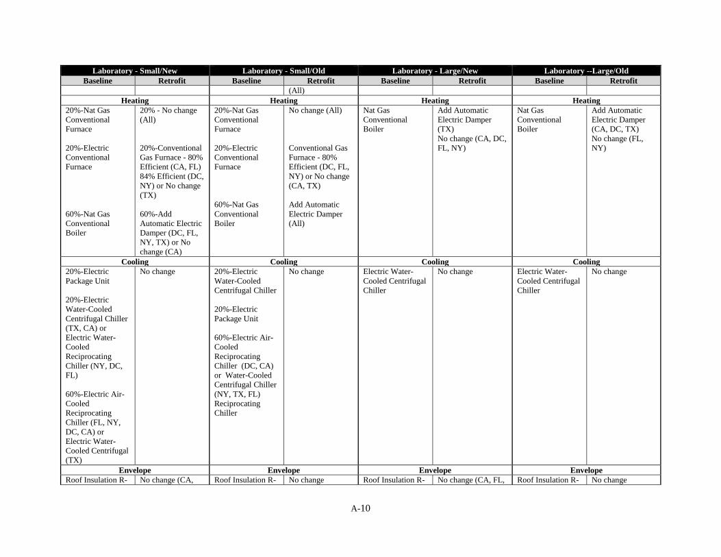
A-10
Laboratory - Small/New Laboratory - Small/Old Laboratory - Large/New Laboratory --Large/Old
Baseline Retrofit Baseline Retrofit Baseline Retrofit Baseline Retrofit
(All)
Heating Heating Heating Heating
20%-Nat Gas
Conventional
Furnace
20%-Electric
Conventional
Furnace
60%-Nat Gas
Conventional
Boiler
20% - No change
(All)
20%-Conventional
Gas Furnace - 80%
Efficient (CA, FL)
84% Efficient (DC,
NY) or No change
(TX)
60%-Add
Automatic Electric
Damper (DC, FL,
NY, TX) or No
change (CA)
20%-Nat Gas
Conventional
Furnace
20%-Electric
Conventional
Furnace
60%-Nat Gas
Conventional
Boiler
No change (All)
Conventional Gas
Furnace - 80%
Efficient (DC, FL,
NY) or No change
(CA, TX)
Add Automatic
Electric Damper
(All)
Nat Gas
Conventional
Boiler
Add Automatic
Electric Damper
(TX)
No change (CA, DC,
FL, NY)
Nat Gas
Conventional
Boiler
Add Automatic
Electric Damper
(CA, DC, TX)
No change (FL,
NY)
Cooling Cooling Cooling Cooling
20%-Electric
Package Unit
20%-Electric
Water-Cooled
Centrifugal Chiller
(TX, CA) or
Electric Water-
Cooled
Reciprocating
Chiller (NY, DC,
FL)
60%-Electric Air-
Cooled
Reciprocating
Chiller (FL, NY,
DC, CA) or
Electric Water-
Cooled Centrifugal
(TX)
No change
20%-Electric
Water-Cooled
Centrifugal Chiller
20%-Electric
Package Unit
60%-Electric Air-
Cooled
Reciprocating
Chiller (DC, CA)
or Water-Cooled
Centrifugal Chiller
(NY, TX, FL)
Reciprocating
Chiller
No change Electric Water-
Cooled Centrifugal
Chiller
No change Electric Water-
Cooled Centrifugal
Chiller
No change
Envelope Envelope Envelope Envelope
Roof Insulation R- No change (CA, Roof Insulation R- No change Roof Insulation R- No change (CA, FL, Roof Insulation R- No change
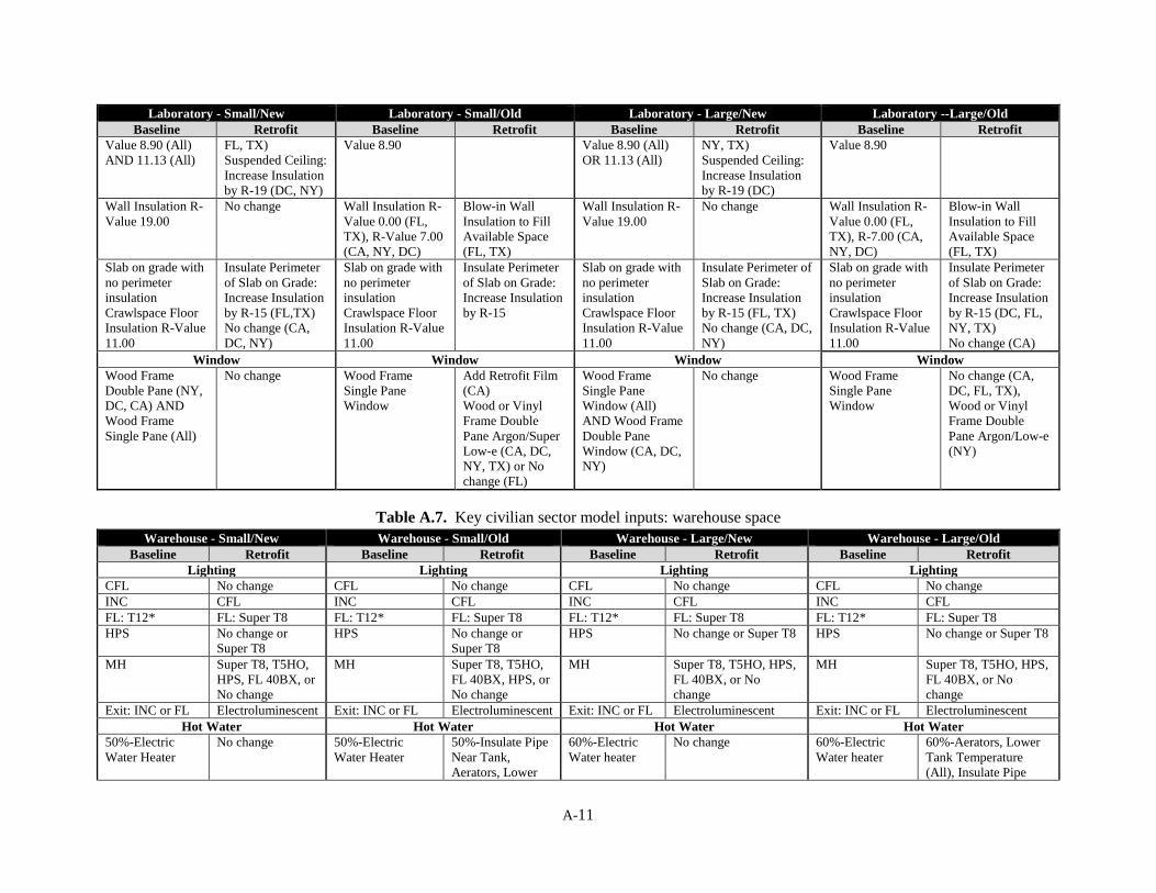
A-11
Laboratory - Small/New Laboratory - Small/Old Laboratory - Large/New Laboratory --Large/Old
Baseline Retrofit Baseline Retrofit Baseline Retrofit Baseline Retrofit
Value 8.90 (All)
AND 11.13 (All)
FL, TX)
Suspended Ceiling:
Increase Insulation
by R-19 (DC, NY)
Value 8.90 Value 8.90 (All)
OR 11.13 (All)
NY, TX)
Suspended Ceiling:
Increase Insulation
by R-19 (DC)
Value 8.90
Wall Insulation R-
Value 19.00
No change Wall Insulation R-
Value 0.00 (FL,
TX), R-Value 7.00
(CA, NY, DC)
Blow-in Wall
Insulation to Fill
Available Space
(FL, TX)
Wall Insulation R-
Value 19.00
No change Wall Insulation R-
Value 0.00 (FL,
TX), R-7.00 (CA,
NY, DC)
Blow-in Wall
Insulation to Fill
Available Space
(FL, TX)
Slab on grade with
no perimeter
insulation
Crawlspace Floor
Insulation R-Value
11.00
Insulate Perimeter
of Slab on Grade:
Increase Insulation
by R-15 (FL,TX)
No change (CA,
DC, NY)
Slab on grade with
no perimeter
insulation
Crawlspace Floor
Insulation R-Value
11.00
Insulate Perimeter
of Slab on Grade:
Increase Insulation
by R-15
Slab on grade with
no perimeter
insulation
Crawlspace Floor
Insulation R-Value
11.00
Insulate Perimeter of
Slab on Grade:
Increase Insulation
by R-15 (FL, TX)
No change (CA, DC,
NY)
Slab on grade with
no perimeter
insulation
Crawlspace Floor
Insulation R-Value
11.00
Insulate Perimeter
of Slab on Grade:
Increase Insulation
by R-15 (DC, FL,
NY, TX)
No change (CA)
Window Window Window Window
Wood Frame
Double Pane (NY,
DC, CA) AND
Wood Frame
Single Pane (All)
No change Wood Frame
Single Pane
Window
Add Retrofit Film
(CA)
Wood or Vinyl
Frame Double
Pane Argon/Super
Low-e (CA, DC,
NY, TX) or No
change (FL)
Wood Frame
Single Pane
Window (All)
AND Wood Frame
Double Pane
Window (CA, DC,
NY)
No change Wood Frame
Single Pane
Window
No change (CA,
DC, FL, TX),
Wood or Vinyl
Frame Double
Pane Argon/Low-e
(NY)
Table A.7. Key civilian sector model inputs: warehouse space
Warehouse - Small/New Warehouse - Small/Old Warehouse - Large/New Warehouse - Large/Old
Baseline Retrofit Baseline Retrofit Baseline Retrofit Baseline Retrofit
Lighting Lighting Lighting Lighting
CFL No change CFL No change CFL No change CFL No change
INC CFL INC CFL INC CFL INC CFL
FL: T12* FL: Super T8 FL: T12* FL: Super T8 FL: T12* FL: Super T8 FL: T12* FL: Super T8
HPS No change or
Super T8
HPS No change or
Super T8
HPS No change or Super T8 HPS No change or Super T8
MH Super T8, T5HO,
HPS, FL 40BX, or
No change
MH Super T8, T5HO,
FL 40BX, HPS, or
No change
MH Super T8, T5HO, HPS,
FL 40BX, or No
change
MH Super T8, T5HO, HPS,
FL 40BX, or No
change
Exit: INC or FL Electroluminescent Exit: INC or FL Electroluminescent Exit: INC or FL Electroluminescent Exit: INC or FL Electroluminescent
Hot Water Hot Water Hot Water Hot Water
50%-Electric
Water Heater
No change
50%-Electric
Water Heater
50%-Insulate Pipe
Near Tank,
Aerators, Lower
60%-Electric
Water heater
No change
60%-Electric
Water heater
60%-Aerators, Lower
Tank Temperature
(All), Insulate Pipe

A-12
Warehouse - Small/New Warehouse - Small/Old Warehouse - Large/New Warehouse - Large/Old
Baseline Retrofit Baseline Retrofit Baseline Retrofit Baseline Retrofit
50%-No Hot
Water
No change
50%-No Hot
Water
Tank Temperature
(CA, DC, FL, NY)
50%-Wrap tank
(CA, NY)
50%-Aerators,
Lower Tank
Temperature (TX)
No change
25%-No Hot
Water
15%-Nat Gas
Water Heater
No change
15%-Wrap Tank with
Insulation (DC, FL) or
No change (CA, NY,
TX)
15%-Nat Gas
Water Heater
25%-No Hot
Water
Near Tank (CA, DC,
FL, NY), Wrap Tank
(CA, NY)
15%-(Gas)Wrap Tank
with Insulation,
Aerators, Lower Tank
Temperature (All)
No change
Heating Heating Heating Heating
50%-Nat Gas
Conventional
Furnace
50%-Not Heated
50%-Nat Gas
Infrared Heating
System - High
Efficiency (DC,
NY) Nat Gas
Infrared Heating
System - Standard
Efficiency (FL),
Electric Infrared
Heating System
(TX), No change
(CA)
No change
50%-Nat Gas
Conventional
Furnace
50%-Not Heated
Nat Gas Infrared
Heating System -
High Efficiency
(DC, NY), Nat
Gas Infrared
Heating System -
Standard
Efficiency (FL),
Electric Infrared
Heating System
(TX), No change
(CA)
No change
60%-Not Heated
25%-Nat Gas
Infrared Heating
System
15%-Nat Gas
Conventional
Furnace
No change
No change
Nat Gas Infrared
Heating System - High
Efficiency (DC, NY),
Nat Gas Infrared
Heating System -
Standard Efficiency
(FL), Electric Infrared
Heating System (TX)
or No change (CA)
60%-Not Heated
25%-Nat Gas
Infrared Heating
System
15%-Nat Gas
Conventional
Furnace
No change
Nat Gas Infrared
Heating System - High
Efficiency (DC, NY)
15%-Nat Gas Infrared
Heating System -
Standard Efficiency
(FL)
15%-Electric Infrared
Heating System (TX)
No change (CA)
Cooling Cooling Cooling Cooling
None No change None No change None No change None No change
Envelope Envelope Envelope Envelope
Roof Insulation
R-Value 14.60
No Change Roof Insulation R-
Value 0.00
No change Roof Insulation
R-Value 13.35
No change Roof Insulation
R-Value 8.90
and 0.00
No change
Wall Insulation
R-Value 9.6
No change Wall Insulation R-
Value 0.00
No change Wall Insulation
R-Value 11.00
and 9.6
No change Wall Insulation
R-Value 0.00
No change
Slab on grade
with no perimeter
insulation
Crawlspace Floor
Insulation R-
Value 11.00
No change Slab on grade with
no perimeter
insulation,
Crawlspace Floor
Insulation R-Value
11.00
No change Slab on grade
with no
perimeter
insulation
Crawlspace
Floor Insulation
No change Slab on grade
with no perimeter
insulation
Crawlspace Floor
Insulation R-
Value 11.00
No change

A-13
Warehouse - Small/New Warehouse - Small/Old Warehouse - Large/New Warehouse - Large/Old
Baseline Retrofit Baseline Retrofit Baseline Retrofit Baseline Retrofit
R-Value 11.00
Window Window Window Window
Wood or Metal
Frame Single-
Pane (All) AND
Wood or Metal
Frame Double
Pane (DC, NY)
No change Wood or Metal
Frame Single Pane
No change Wood or Metal
Frame Single
Pane (All) AND
Wood or Metal
Frame Double-
Pane (DC, NY)
No change Wood or Metal
Frame Single
Pane Frame
No change

A-14
Table A.8. Baseline energy consumption proportions by end use (site basis)
Characteristics Space
Heating
Space
Cooling Ventilation Lighting
Hot
Water All Other
Healthcare 4.9% 12.8% 8.2% 13.2% 24.6% 36.4%
Avg Vintage 1994 5.2% 14.4% 1.1% 14.1% 26.3% 38.9%
Large 4.8% 13.9% 1.1% 12.8% 27.4% 40.0%
Small 8.4% 17.7% 1.3% 24.6% 17.7% 30.2%
Avg Vintage 1957 4.7% 11.4% 14.4% 12.3% 23.1% 34.1%
Large 4.3% 11.0% 15.0% 11.0% 23.8% 34.8%
Small 8.6% 14.4% 9.0% 23.4% 16.5% 28.1%
Lab 5.1% 17.8% 0.2% 11.9% 15.9% 49.2%
Avg Vintage 1994 4.8% 18.7% 0.3% 11.6% 15.8% 48.8%
Large 3.9% 16.1% 0.3% 11.4% 17.3% 51.0%
Small 5.8% 21.6% 0.2% 11.7% 14.3% 46.4%
Avg Vintage 1957 5.3% 17.0% 0.1% 12.2% 15.9% 49.5%
Large 3.8% 14.4% 0.0% 11.2% 17.0% 53.6%
Small 7.1% 20.0% 0.3% 13.2% 14.6% 44.8%
Office 7.1% 12.4% 0.3% 26.5% 22.9% 30.8%
Avg Vintage 1994 7.0% 13.0% 0.3% 25.8% 23.0% 30.9%
Large 6.6% 11.7% 0.3% 28.8% 22.5% 30.2%
Medium 7.7% 16.9% 0.5% 16.2% 25.1% 33.6%
Small 16.2% 21.2% 0.8% 15.8% 19.6% 26.3%
Avg Vintage 1957 7.2% 11.8% 0.4% 27.2% 22.8% 30.6%
Large 6.8% 10.7% 0.3% 30.0% 22.3% 29.9%
Medium 8.1% 14.7% 0.6% 18.2% 25.0% 33.5%
Small 15.8% 22.0% 1.0% 17.7% 18.6% 25.0%
Warehouse 25.4% 0.0% 0.2% 0.7% 35.3% 38.4%
Avg Vintage 1994 25.3% 0.0% 0.2% 0.6% 35.4% 38.4%
Large 24.8% 0.0% 0.2% 0.4% 35.8% 38.9%
Small 29.5% 0.0% 0.4% 2.0% 32.7% 35.5%
Avg Vintage 1957 25.5% 0.0% 0.2% 0.7% 35.3% 38.3%
Large 24.9% 0.0% 0.2% 0.5% 35.7% 38.8%
Small 29.6% 0.0% 0.4% 2.4% 32.4% 35.2%
Table A.9. Vintages of DOD building stock modeled by region (percent of GSF)
Vintage DC FL NY CA TX
1930s 14% 15% 0% 0% 0%
1940s 8% 4% 24% 3% 3%
1950s 11% 20% 0% 7% 7%
1960s 20% 17% 1% 17% 17%
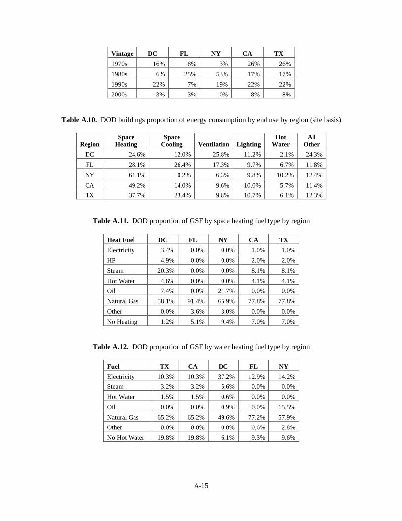
A-15
Vintage DC FL NY CA TX
1970s 16% 8% 3% 26% 26%
1980s 6% 25% 53% 17% 17%
1990s 22% 7% 19% 22% 22%
2000s 3% 3% 0% 8% 8%
Table A.10. DOD buildings proportion of energy consumption by end use by region (site basis)
Region
Space
Heating
Space
Cooling Ventilation Lighting
Hot
Water
All
Other
DC 24.6% 12.0% 25.8% 11.2% 2.1% 24.3%
FL 28.1% 26.4% 17.3% 9.7% 6.7% 11.8%
NY 61.1% 0.2% 6.3% 9.8% 10.2% 12.4%
CA 49.2% 14.0% 9.6% 10.0% 5.7% 11.4%
TX 37.7% 23.4% 9.8% 10.7% 6.1% 12.3%
Table A.11. DOD proportion of GSF by space heating fuel type by region
Heat Fuel DC FL NY CA TX
Electricity 3.4% 0.0% 0.0% 1.0% 1.0%
HP 4.9% 0.0% 0.0% 2.0% 2.0%
Steam 20.3% 0.0% 0.0% 8.1% 8.1%
Hot Water 4.6% 0.0% 0.0% 4.1% 4.1%
Oil 7.4% 0.0% 21.7% 0.0% 0.0%
Natural Gas 58.1% 91.4% 65.9% 77.8% 77.8%
Other 0.0% 3.6% 3.0% 0.0% 0.0%
No Heating 1.2% 5.1% 9.4% 7.0% 7.0%
Table A.12. DOD proportion of GSF by water heating fuel type by region
Fuel TX CA DC FL NY
Electricity 10.3% 10.3% 37.2% 12.9% 14.2%
Steam 3.2% 3.2% 5.6% 0.0% 0.0%
Hot Water 1.5% 1.5% 0.6% 0.0% 0.0%
Oil 0.0% 0.0% 0.9% 0.0% 15.5%
Natural Gas 65.2% 65.2% 49.6% 77.2% 57.9%
Other 0.0% 0.0% 0.0% 0.6% 2.8%
No Hot Water 19.8% 19.8% 6.1% 9.3% 9.6%
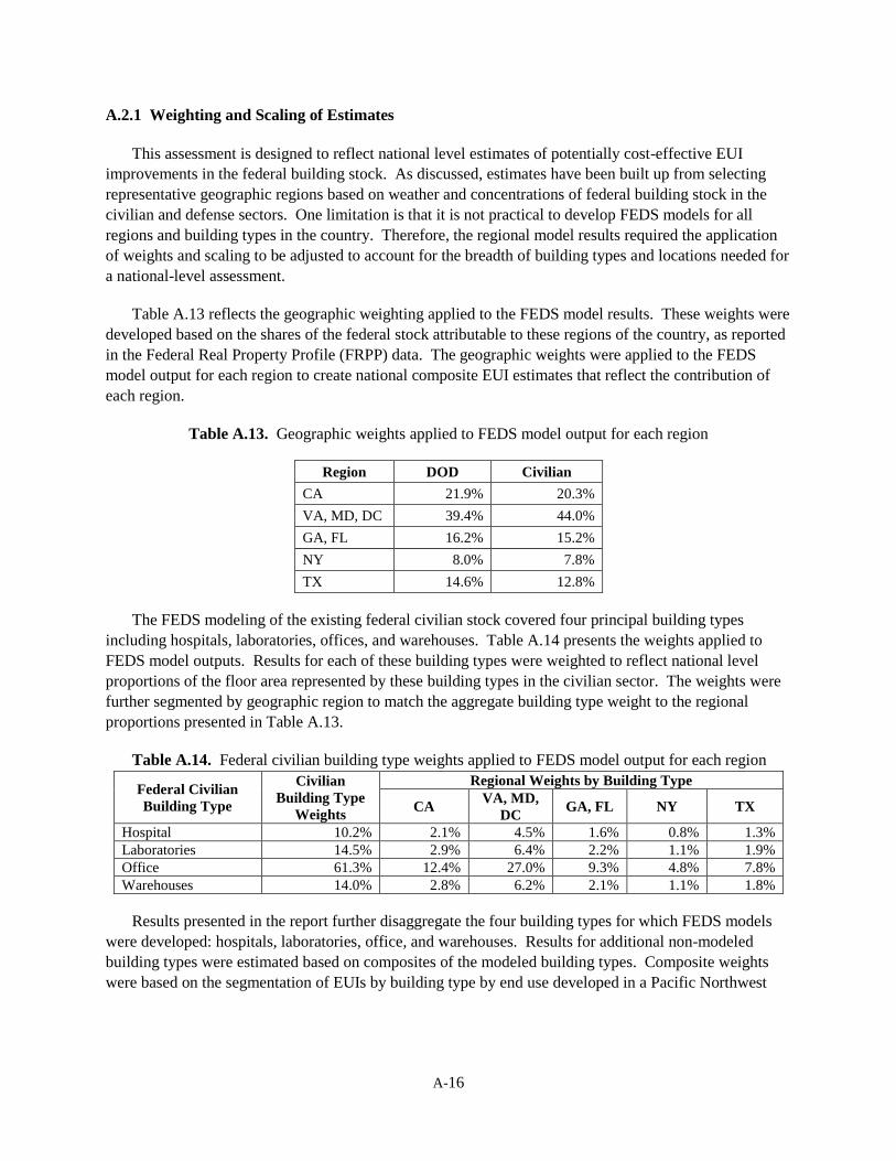
A-16
A.2.1 Weighting and Scaling of Estimates
This assessment is designed to reflect national level estimates of potentially cost-effective EUI
improvements in the federal building stock. As discussed, estimates have been built up from selecting
representative geographic regions based on weather and concentrations of federal building stock in the
civilian and defense sectors. One limitation is that it is not practical to develop FEDS models for all
regions and building types in the country. Therefore, the regional model results required the application
of weights and scaling to be adjusted to account for the breadth of building types and locations needed for
a national-level assessment.
Table A.13 reflects the geographic weighting applied to the FEDS model results. These weights were
developed based on the shares of the federal stock attributable to these regions of the country, as reported
in the Federal Real Property Profile (FRPP) data. The geographic weights were applied to the FEDS
model output for each region to create national composite EUI estimates that reflect the contribution of
each region.
Table A.13. Geographic weights applied to FEDS model output for each region
Region DOD Civilian
CA 21.9% 20.3%
VA, MD, DC 39.4% 44.0%
GA, FL 16.2% 15.2%
NY 8.0% 7.8%
TX 14.6% 12.8%
The FEDS modeling of the existing federal civilian stock covered four principal building types
including hospitals, laboratories, offices, and warehouses. Table A.14 presents the weights applied to
FEDS model outputs. Results for each of these building types were weighted to reflect national level
proportions of the floor area represented by these building types in the civilian sector. The weights were
further segmented by geographic region to match the aggregate building type weight to the regional
proportions presented in Table A.13.
Table A.14. Federal civilian building type weights applied to FEDS model output for each region
Federal Civilian
Building Type
Civilian
Building Type
Weights
Regional Weights by Building Type
CA VA, MD,
DC GA, FL NY TX
Hospital 10.2% 2.1% 4.5% 1.6% 0.8% 1.3%
Laboratories 14.5% 2.9% 6.4% 2.2% 1.1% 1.9%
Office 61.3% 12.4% 27.0% 9.3% 4.8% 7.8%
Warehouses 14.0% 2.8% 6.2% 2.1% 1.1% 1.8%
Results presented in the report further disaggregate the four building types for which FEDS models
were developed: hospitals, laboratories, office, and warehouses. Results for additional non-modeled
building types were estimated based on composites of the modeled building types. Composite weights
were based on the segmentation of EUIs by building type by end use developed in a Pacific Northwest

A-17
National Laboratory (PNNL) study18
for the Federal Energy Management Program (FEMP). Table A.15
presents the composite proportions used to extend the civilian building type results from the modeled
building types to the additional building types presented in the report.
Table A.15. Federal civilian building type composites used to extend modeled EUIs to non-
modeled building types
Modeled
Types
Non-Modeled Building Types
Service School Other Prison Industrial
Storage 36.5% 8.1% 12.1% 0 39.3%
Office 63.5% 71.9% 87.9% 0 0
Hospital 0 0 0 85.0% 0
Research & Development 0 0 0 0 60.7%
Finally, the FEDS modeled results for DOD and civilian buildings were based on actual calibrated
studies in the case of DOD facilities, and federal civilian prototype buildings for the civilian sector.
Using the estimated baseline EUIs for just these facilities and building types would not be expected to
match the weighted average aggregate EUI reported by FEMP for each sector’s goal-subject floor area.
Therefore, it is necessary to simply scale the modeled results to the reported goal-subject aggregate EUI
for DOD and civilian buildings. Table A.16 presents those scaling factors.
Table A.16. Factors applied to modeled EUIs to scale to FEMP
reported goal-subject baseline EUIs
Sector Scaling
Factor
Civilian 1.399
DOD 0.754
Total Federal 0.919
A.2 Cost Assumptions
The following tables present the electricity and gas rates used in the FEDS analysis. DOD natural gas
and electricity rates were derived from data reported in the Army Energy and Water Reporting System
(AEWRS) during fiscal year 2013 for the specific site modeled. It was assumed that these rates were
representative for the region that each site represents. Natural gas and electricity rates for the civilian
sector came based on calendar year 2012 and came from utilities in the five geographic regions where the
prototype buildings were based.
18
Judd KS, AR Kora, JW Henderson, BJ Russo, J Katz, M Hummon, and EM Rauch. 2010. Roadmap to a Climate Neutral Federal Government. PNNL-19643, Pacific Northwest National Laboratory, Richland, WA.

A-18
Table A.17. Regional natural gas rates used in the analysis
Region Civilian DOD
$/therm $/therm
CA 0.78 0.56
DC 1.14 0.28
FL 1.01 0.65
NY 0.92 0.55
TX 0.75 0.40
Table A.18. Electricity rates used for the civilian sector analysis
CA Winter
Weekdays
Period
Start
Time
End
Time
Energy
Rate Units
Demand
Rate Units
1 800 2100 15.73 cents/kWh 9.7 $/kW
2 2100 800 12.47 cents/kWh 0 $/kW
Weekends
1 100 100 12.47 cents/kWh 0 $/kW
CA Summer
Weekdays
1 800 1200 16.1 cents/kWh 14.86 $/kW
2 1200 1800 22.06 cents/kWh 26.58 $/kW
3 1800 2300 16.1 cents/kWh 14.86 $/kW
4 2300 800 12.84 cents/kWh 9.7 $/kW
Weekends
1 100 100 5.02 cents/kWh 0 $/kW
DC Winter
Weekdays
1 700 2200 9.25 cents/kWh 11.11 $/kW
2 2200 700 6.61 cents/kWh 0 $/kW
Weekends
1 100 100 6.61 cents/kWh 0 $/kW
DC Summer
Weekdays
1 1000 2200 9.25 cents/kWh 12.52 $/kW
2 2200 1000 6.61 cents/kWh 0 $/kW
Weekends
1 100 100 6.61 cents/kWh 0 $/kW
FL Winter
Weekdays
1 100 100 6.13 cents/kWh 4.32 $/kW
Weekends
1 100 100 6.13 cents/kWh 0 $/kW
FL Summer
Weekdays
1 2100 1200 6.56 cents/kWh 0 $/kW
2 1200 1400 9.79 cents/kWh 4.32 $/kW
3 1400 1900 15.39 cents/kWh 12.93 $/kW
4 1900 2100 9.79 cents/kWh 4.32 $/kW
Weekends

A-19
1 2200 1100 3.32 cents/kWh 0 $/kW
2 1100 2200 5.41 cents/kWh 0 $/kW
TX All Months
All Days
1 1400 1900 15.85 cents/kWh 6.35 $/kW
2 1900 1400 3.35 cents/kWh 0 $/kW
NY Winter
Weekdays
1 700 2300 12.56 cents/kWh 3.58 $/kW
2 2300 700 11.17 cents/kWh 0 $/kW
Weekends
1 100 100 11.17 cents/kWh 0 $/kW
NY Summer
Weekdays
1 700 2300 12.56 cents/kWh 3.58 $/kW
2 2300 700 11.17 cents/kWh 0 $/kW
Weekends
1 100 100 11.17 cents/kWh 0 $/kW
Table A.19. Electricity rates used for the DOD sector analysis
CA Winter
Weekdays
Period
Start
Time
End
Time
Energy
Rate Units
Demand
Rate Units
1 800 1700 7.24 cents/kWh 6.27 $/kW
2 1700 800 5.56 cents/kWh 0 $/kW
Weekends
1 100 100 5.56 cents/kWh 0 $/kW
CA Summer
Weekdays
1 800 1200 6.95 cents/kWh 4.93 $/kW
2 1200 1800 10.94 cents/kWh 24.73 $/kW
3 1800 2300 6.95 cents/kWh 4.93 $/kW
4 2300 800 5.02 cents/kWh 0 $/kW
Weekends
1 100 100 5.02 cents/kWh 0 $/kW
DC Winter
Weekdays
1 700 2200 2.99 cents/kWh 13.97 $/kW
2 2200 700 2.86 cents/kWh 0 $/kW
Weekends
1 600 600 2.86 cents/kWh 0 $/kW
DC Summer
Weekdays
1 1000 2200 2.99 cents/kWh 13.97 $/kW
2 2200 1000 2.86 cents/kWh 0 $/kW
Weekends
1 600 600 2.86 cents/kWh 0 $/kW
FL Winter
Weekdays
1 700 2300 3.86 cents/kWh 0 $/kW
2 2300 700 3.04 cents/kWh 0 $/kW
Weekends
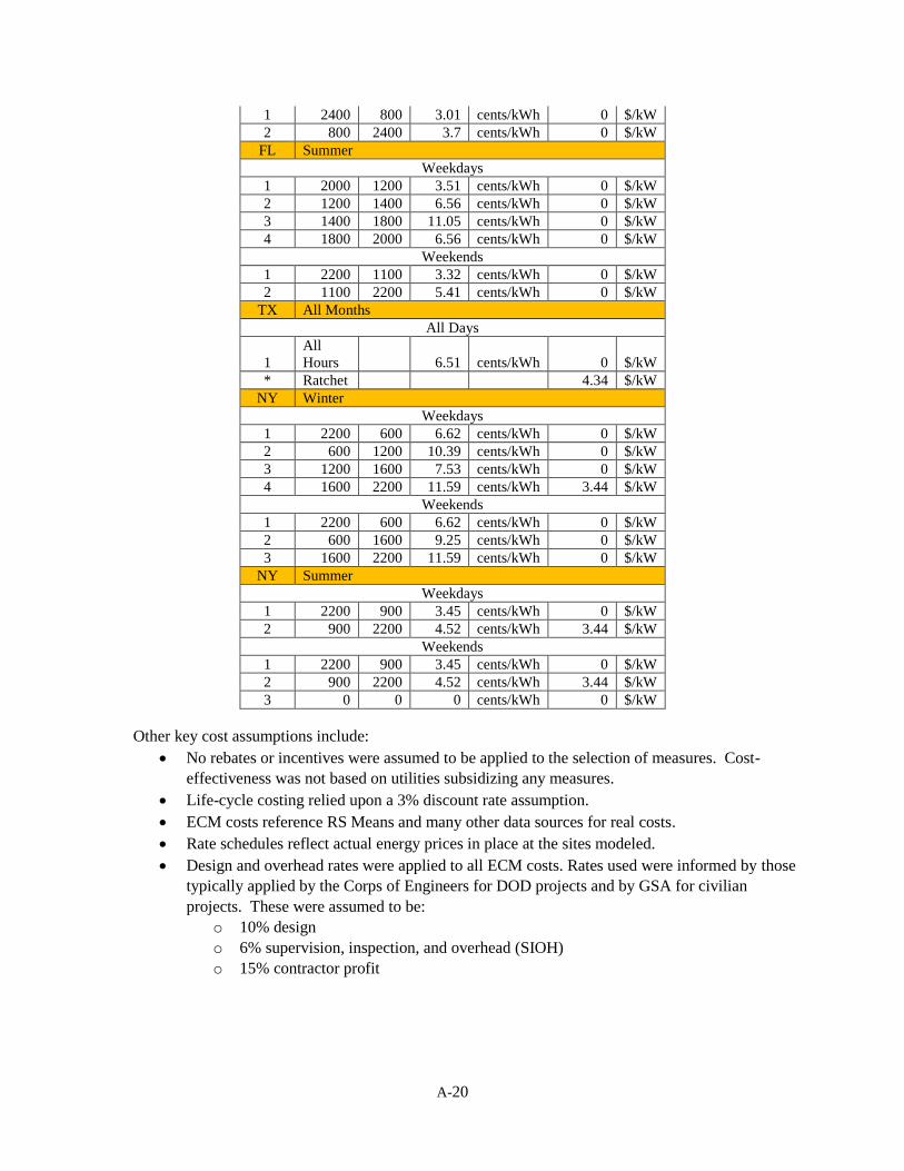
A-20
1 2400 800 3.01 cents/kWh 0 $/kW
2 800 2400 3.7 cents/kWh 0 $/kW
FL Summer
Weekdays
1 2000 1200 3.51 cents/kWh 0 $/kW
2 1200 1400 6.56 cents/kWh 0 $/kW
3 1400 1800 11.05 cents/kWh 0 $/kW
4 1800 2000 6.56 cents/kWh 0 $/kW
Weekends
1 2200 1100 3.32 cents/kWh 0 $/kW
2 1100 2200 5.41 cents/kWh 0 $/kW
TX All Months
All Days
1
All
Hours 6.51 cents/kWh 0 $/kW
* Ratchet 4.34 $/kW
NY Winter
Weekdays
1 2200 600 6.62 cents/kWh 0 $/kW
2 600 1200 10.39 cents/kWh 0 $/kW
3 1200 1600 7.53 cents/kWh 0 $/kW
4 1600 2200 11.59 cents/kWh 3.44 $/kW
Weekends
1 2200 600 6.62 cents/kWh 0 $/kW
2 600 1600 9.25 cents/kWh 0 $/kW
3 1600 2200 11.59 cents/kWh 0 $/kW
NY Summer
Weekdays
1 2200 900 3.45 cents/kWh 0 $/kW
2 900 2200 4.52 cents/kWh 3.44 $/kW
Weekends
1 2200 900 3.45 cents/kWh 0 $/kW
2 900 2200 4.52 cents/kWh 3.44 $/kW
3 0 0 0 cents/kWh 0 $/kW
Other key cost assumptions include:
No rebates or incentives were assumed to be applied to the selection of measures. Cost-
effectiveness was not based on utilities subsidizing any measures.
Life-cycle costing relied upon a 3% discount rate assumption.
ECM costs reference RS Means and many other data sources for real costs.
Rate schedules reflect actual energy prices in place at the sites modeled.
Design and overhead rates were applied to all ECM costs. Rates used were informed by those
typically applied by the Corps of Engineers for DOD projects and by GSA for civilian
projects. These were assumed to be:
o 10% design
o 6% supervision, inspection, and overhead (SIOH)
o 15% contractor profit

A-21
A.3 Selection of Cost-effective ECMs
A.3.1 Civilian Buildings
Table A.20 lists the ECMs selected as cost-effective by the FEDS model for the major civilian
building types modeled. Each measure’s simple payback period and savings-to-investment ratio (SIR) is
provided as a basis for comparison of measures. Because the FEDS-based analysis was designed to
reflect the major climate regions and representative federal building stock regions, this list reflects the list
of measures expected to cost-effective at the national average. Not all measures listed will be cost-
effective in all areas, but all would be cost-effective in the locations where the FEDS model estimates
they would, based on the state of the existing stock, prevailing electric tariffs, fossil fuel rates, and
baseline operating regimes.
The intent of the tables below is to list the measures FEDS found cost effective and illustrate at the
summary level, what the economic impacts would be from their adoption at the modeled sites/buildings.
Because the following tables represent a composite of all retrofits across modeled building types and
regions, in some cases, retrofits shown in the table will reflect shorter paybacks for higher-end (more
expensive) technologies. This is a result of the cost-effectiveness thresholds being different under
differing climate and utility price regimes, and the resulting impact being higher for a specific technology
at one site than at another. For example, in Table A.20, a gas boiler with an 84 percent efficiency has a
weighted average simple payback of 14.8 years, while one with a 91 percent efficiency has a payback of
10.7 years. This is counterintuitive, but correct, given that the table is combining the impacts across all
sites, vintages, types, and sizes.
Tables A.20 and A.21 present the measures selected from the FEDS analysis as well the estimated
energy savings, SIR and simple payback by energy end use and ECM. These values have not been fully
weighted or scaled to all civilian building types and locations or DOD locations. The derived payback in
Table 7 in the body of the report was calculated based on the fully weighted energy analysis, which is
why aggregate average payback for civilian and DOD investments are slightly different. The tables below
are included to provide some numerical insight for comparing between the measures.
Naming conventions for the measures in the table below can be found in the FEDS User Guide at:
http://www.pnl.gov/feds/pdfs/FEDS_6-0_user_guide.pdf.
Table A.20. Federal civilian buildings national average cost-effective ECMs
Cost-Effective ECMs by End Use
Percent of
Aggregate
Energy
Savings
Energy
Savings-
Weighted
Avg SIR
Energy
Savings-
Weighted
Avg Simple
Payback
Floor 1.8% 4.3 4.9
Insulate Perimeter of Slab on Grade: Increase Insulation by R-10 0.0% 1.8 8.6
Insulate Perimeter of Slab on Grade: Increase Insulation by R-15 1.8% 4.3 4.9
Insulate Perimeter of Slab on Grade: Increase Insulation by R-7.5 0.0% 3.0 4.0
Windows 17.8% 1.6 11.8
Add Retrofit Film 0.2% 1.7 6.1
Install Thermal Break Aluminum Frame Double Pane Argon/Super Low-e
Window 2.2% 1.4 14.3
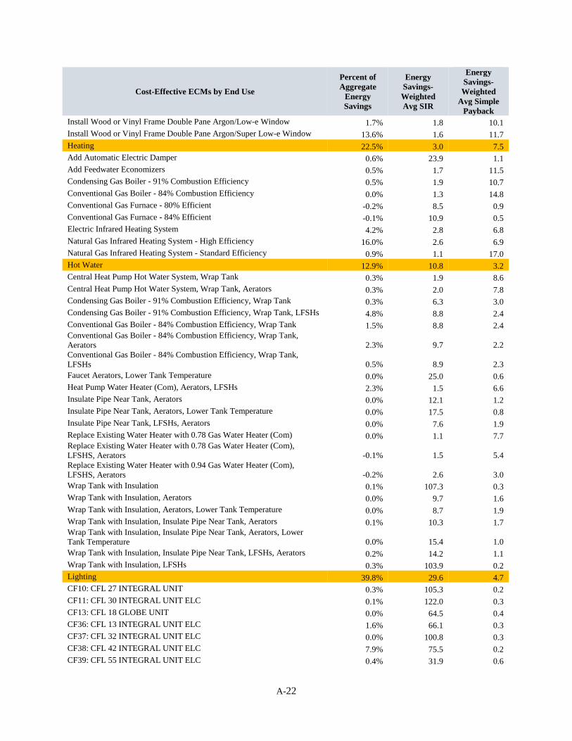
A-22
Cost-Effective ECMs by End Use
Percent of
Aggregate
Energy
Savings
Energy
Savings-
Weighted
Avg SIR
Energy
Savings-
Weighted
Avg Simple
Payback
Install Wood or Vinyl Frame Double Pane Argon/Low-e Window 1.7% 1.8 10.1
Install Wood or Vinyl Frame Double Pane Argon/Super Low-e Window 13.6% 1.6 11.7
Heating 22.5% 3.0 7.5
Add Automatic Electric Damper 0.6% 23.9 1.1
Add Feedwater Economizers 0.5% 1.7 11.5
Condensing Gas Boiler - 91% Combustion Efficiency 0.5% 1.9 10.7
Conventional Gas Boiler - 84% Combustion Efficiency 0.0% 1.3 14.8
Conventional Gas Furnace - 80% Efficient -0.2% 8.5 0.9
Conventional Gas Furnace - 84% Efficient -0.1% 10.9 0.5
Electric Infrared Heating System 4.2% 2.8 6.8
Natural Gas Infrared Heating System - High Efficiency 16.0% 2.6 6.9
Natural Gas Infrared Heating System - Standard Efficiency 0.9% 1.1 17.0
Hot Water 12.9% 10.8 3.2
Central Heat Pump Hot Water System, Wrap Tank 0.3% 1.9 8.6
Central Heat Pump Hot Water System, Wrap Tank, Aerators 0.3% 2.0 7.8
Condensing Gas Boiler - 91% Combustion Efficiency, Wrap Tank 0.3% 6.3 3.0
Condensing Gas Boiler - 91% Combustion Efficiency, Wrap Tank, LFSHs 4.8% 8.8 2.4
Conventional Gas Boiler - 84% Combustion Efficiency, Wrap Tank 1.5% 8.8 2.4
Conventional Gas Boiler - 84% Combustion Efficiency, Wrap Tank,
Aerators 2.3% 9.7 2.2
Conventional Gas Boiler - 84% Combustion Efficiency, Wrap Tank,
LFSHs 0.5% 8.9 2.3
Faucet Aerators, Lower Tank Temperature 0.0% 25.0 0.6
Heat Pump Water Heater (Com), Aerators, LFSHs 2.3% 1.5 6.6
Insulate Pipe Near Tank, Aerators 0.0% 12.1 1.2
Insulate Pipe Near Tank, Aerators, Lower Tank Temperature 0.0% 17.5 0.8
Insulate Pipe Near Tank, LFSHs, Aerators 0.0% 7.6 1.9
Replace Existing Water Heater with 0.78 Gas Water Heater (Com) 0.0% 1.1 7.7
Replace Existing Water Heater with 0.78 Gas Water Heater (Com),
LFSHS, Aerators -0.1% 1.5 5.4
Replace Existing Water Heater with 0.94 Gas Water Heater (Com),
LFSHS, Aerators -0.2% 2.6 3.0
Wrap Tank with Insulation 0.1% 107.3 0.3
Wrap Tank with Insulation, Aerators 0.0% 9.7 1.6
Wrap Tank with Insulation, Aerators, Lower Tank Temperature 0.0% 8.7 1.9
Wrap Tank with Insulation, Insulate Pipe Near Tank, Aerators 0.1% 10.3 1.7
Wrap Tank with Insulation, Insulate Pipe Near Tank, Aerators, Lower
Tank Temperature 0.0% 15.4 1.0
Wrap Tank with Insulation, Insulate Pipe Near Tank, LFSHs, Aerators 0.2% 14.2 1.1
Wrap Tank with Insulation, LFSHs 0.3% 103.9 0.2
Lighting 39.8% 29.6 4.7
CF10: CFL 27 INTEGRAL UNIT 0.3% 105.3 0.2
CF11: CFL 30 INTEGRAL UNIT ELC 0.1% 122.0 0.3
CF13: CFL 18 GLOBE UNIT 0.0% 64.5 0.4
CF36: CFL 13 INTEGRAL UNIT ELC 1.6% 66.1 0.3
CF37: CFL 32 INTEGRAL UNIT ELC 0.0% 100.8 0.3
CF38: CFL 42 INTEGRAL UNIT ELC 7.9% 75.5 0.2
CF39: CFL 55 INTEGRAL UNIT ELC 0.4% 31.9 0.6

A-23
Cost-Effective ECMs by End Use
Percent of
Aggregate
Energy
Savings
Energy
Savings-
Weighted
Avg SIR
Energy
Savings-
Weighted
Avg Simple
Payback
CF4: CFL 15 INTEGRAL UNIT ELC 0.2% 61.6 0.5
CF5: CFL 18 INTEGRAL UNIT ELC 1.6% 61.2 0.3
CF6: CFL 20 INTEGRAL UNIT ELC 0.2% 86.3 0.3
CF9: CFL 26 INTEGRAL UNIT ELC 3.0% 66.6 0.3
EX11: EXIT - ELECTROLUMINESCENT PANEL 1.0% 15.2 1.5
EX12: EXIT - ELECTROLUMINESCENT PANEL RETRO KIT 1.5% 16.9 1.3
FL244: FL 2X4 4F32T8 ELC4 0.4% 2.2 8.1
FL263: FL 2X2 2F14T5 ELC2 REF 1.4% 5.5 4.2
FL273: FL 2X4 4F54T5HO ELC2 REF 0.3% 1.6 11.1
FL275: FL 2X4 2F32ST8 ELC2 0.3% 1.6 10.0
FL276: FL 2X4 3F32ST8 ELC3 0.1% 2.3 7.0
FL279: FL 2X4 2F32ST8 ELC2 REF 0.7% 1.4 11.9
FL280: FL 2X4 3F32ST8 ELC3 REF 6.7% 2.8 7.1
FL283: FL 2X4 2F30ST8 ELC2 2.6% 2.3 7.9
FL283: FL 2X4 2F30ST8 ELC2 (Component Repl.) 2.1% 1.5 11.3
FL284: FL 2X4 3F30ST8 ELC3 0.2% 3.6 4.5
FL284: FL 2X4 3F30ST8 ELC3 (Component Repl.) 1.2% 1.3 12.4
FL285: FL 2X4 4F30ST8 ELC2 0.0% 1.4 12.5
FL287: FL 2X4 2F30ST8 ELC2 REF (Component Repl.) 0.0% 1.1 15.0
FL288: FL 2X4 3F30ST8 ELC3 REF 1.2% 2.0 8.6
FL289: FL 2X4 4F30ST8 ELC2 REF 1.3% 3.4 5.3
FL303: FL 2X4 2F25ST8 ELC2 REF 1.1% 1.7 10.4
FL304: FL 2X4 3F25ST8 ELC3 REF 0.3% 3.4 4.9
FL309: FL 2X3 6F40BX ELC2 REF 0.2% 2.1 8.1
FL52: FL 1X4 2F32T8 ELC2 1.8% 2.5 7.3
FL53: FL 1X4 1F32T8 ELC1 0.1% 10.3 2.3
HS18: HPS 310 PEND 0.0% 1.2 14.6
HS97: HPS 70 WALL ELC 0.0% 1.1 15.8
MH67: MH 150 HE WALL ELC 0.0% 2.6 6.6
Roof 0.7% 1.3 12.3
Attic Ceiling: Increase Insulation by R-19 (blow-in cellulose) 0.0% 1.5 7.8
Suspended Ceiling: Increase Insulation by R-19 0.5% 1.2 12.6
Suspended Ceiling: Increase Insulation by R-38 0.2% 1.6 11.6
Wall 4.5% 2.4 8.1
Blow-in Wall Insulation to Fill Available Space 4.5% 2.4 8.1
Grand Total 100.0% 14.3 6.6
A.3.2 DOD Buildings
Table A.21 lists the ECMs selected as cost-effective by the FEDS model for the DOD sites modeled.
Each measure’s simple payback period and savings-to-investment ratio (SIR) is provided as a basis for
comparison of measures. Because the FEDS-based analysis was designed to reflect the major climate
regions and representative federal building stock regions, this list reflects the list of measures expected to
cost-effective at the national average. Not all measures listed will be cost-effective in all areas, but all
would be cost-effective in the locations where the FEDS model estimates they would, based on the state
of the existing stock, prevailing electric tariffs, fossil fuel rates, and baseline operating regimes.

A-24
The intent of the tables below is to list the measures FEDS found cost effective and illustrate at the
summary level, what the economic impacts would be from their adoption at the modeled sites/buildings.
Because the following tables represent a composite of all modeled retrofits across building types and
regions, in some cases, retrofits shown in the table will reflect shorter paybacks for higher-end (more
expensive) technologies. This is a result of the cost-effectiveness thresholds being different under
differing climate and utility price regimes, and the resulting impact being higher for a specific technology
at one site than at another. For example, in Table A.21, increasing attic insulation to R-13 has a weighted
average simple payback of 12.0 years, while increasing to R-38 has a payback of 2.4 years. This is
counterintuitive, but correct, given that the table is combining the impacts across all sites, vintages, types,
and sizes. So for example, in some places (TX/CA/FL) it would be technically cost efficient to go to R-
13 blown-in attic insulation, but no further. Going to R-13 from nothing in those areas would have a
relatively long payback because there are some but not a lot of savings. However, in northern climates it
is cost effective to go to R-38 and the savings are so substantial (going from no or very little insulation to
R-38) that the payback is much shorter.
Table A.21. DOD facilities national average cost-effective ECMs
Cost-Effective ECMs by End Use
Percent of
Aggregate
Energy
Savings
Energy
Savings-
Weighted Avg
SIR
Energy
Savings-
Weighted Avg
Simple
Payback
Floor 2.7% 1.9 10.3
Insulate Perimeter of Slab on Grade: Increase Insulation by R-10 0.6% 1.5 12.5
Insulate Perimeter of Slab on Grade: Increase Insulation by R-15 2.1% 2.0 9.7
Windows 3.0% 1.2 11.8
Add Retrofit Film 0.0% 1.3 4.1
Install Aluminum Frame Double Pane Argon/Low-e Window 0.1% 1.0 19.1
Install Aluminum Frame Double Pane Argon/Super Low-e Window 1.1% 1.2 12.0
Install Thermal Break Aluminum Frame Double Pane Argon/Super
Low-e Window
1.7% 1.3 11.5
Heating 17.7% 4.3 10.5
Add Automatic Electric Damper 1.3% 8.5 2.9
Condensing Gas Furnace - 90% Efficient 0.0% 22.7 0.9
Condensing Gas Furnace - 92% Efficient 0.0% 11.0 1.4
Conventional Gas Boiler - 80% Combustion Efficiency 0.1% 9.9 4.8
Conventional Gas Boiler - 84% Combustion Efficiency 0.2% 3.1 10.3
Conventional Gas Furnace - 80% Efficient 0.4% 25.5 0.8
Conventional Gas Furnace - 84% Efficient 0.0% 29.1 0.5
Electric Infrared Heating System 2.6% 3.2 7.8
Natural Gas Infrared Heating System - High Efficiency 4.3% 5.4 8.8
Natural Gas Infrared Heating System - Medium Efficiency 4.5% 1.8 14.1
Natural Gas Infrared Heating System - Standard Efficiency 4.3% 3.3 13.4
HEATING/Cooling 0.2% 1.0 12.5
High Efficiency Electric Air Source Heat Pump (Commercial) 0.3% 1.1 11.4
Standard Efficiency Packaged Terminal AC Unit (PTAC) with Electric
Resistance Heat
-0.1% 1.4 6.9
Hot Water 7.2% 37.8 1.2
Central Heat Pump Hot Water System, Wrap Tank, LFSHs 0.1% 1.4 9.4
Condensing Gas Boiler - 91% Combustion Efficiency, Wrap Tank 0.2% 4.5 5.8
Condensing Gas Boiler - 91% Combustion Efficiency, Wrap Tank,
LFSHs
0.1% 11.5 2.2

A-25
Cost-Effective ECMs by End Use
Percent of
Aggregate
Energy
Savings
Energy
Savings-
Weighted Avg
SIR
Energy
Savings-
Weighted Avg
Simple
Payback
Condensing Gas Boiler - 91% Combustion Efficiency, Wrap Tank,
LFSHs, Aerators
0.2% 8.9 2.7
Conventional Gas Boiler - 80% Combustion Efficiency, Wrap Tank 0.0% 7.6 2.2
Conventional Gas Boiler - 80% Combustion Efficiency, Wrap Tank,
LFSHs
0.0% 56.8 0.3
Conventional Gas Boiler - 81.5% Combustion Efficiency, Wrap Tank 0.0% 14.4 1.2
Conventional Gas Boiler - 84% Combustion Efficiency, Wrap Tank 0.1% 9.3 2.1
Conventional Gas Boiler - 84% Combustion Efficiency, Wrap Tank,
Aerators
0.0% 11.1 1.6
Conventional Gas Boiler - 84% Combustion Efficiency, Wrap Tank,
LFSHs
0.1% 11.0 1.8
Conventional Gas Boiler - 84% Combustion Efficiency, Wrap Tank,
LFSHs, Aerators
0.6% 11.1 2.5
Faucet Aerators 0.0% 38.2 1.2
Faucet Aerators, Lower Tank Temperature 0.1% 48.4 0.9
Insulate Pipe Near Tank, LFSHs 0.0% 20.5 0.8
Insulate Pipe Near Tank, LFSHs, Lower Tank Temperature 0.0% 1.5 10.4
LFSHs, Aerators, Lower Tank Temperature 0.0% 7.1 2.2
Low-Flow Showerheads (LFSHs) 0.0% 98.3 1.0
Low-Flow Showerheads (LFSHs), Aerators 0.0% 49.9 0.3
Low-Flow Showerheads (LFSHs), Lower Tank Temperature 0.0% 8.8 4.5
Replace Existing Water Heater with 0.78 Gas Water Heater (Com),
LFSHs, Lower Tank Temp.
0.0% 1.9 4.6
Replace Existing Water Heater with 0.94 Gas Water Heater (Com),
LFSHS, Aerators
0.2% 6.0 1.4
Replace Existing Water Heater with 0.94 Gas Water Heater (Com),
LFSHs, Lower Tank Temp.
0.0% 2.6 3.3
Wrap Tank with Insulation 2.1% 68.9 0.3
Wrap Tank with Insulation, Aerators 0.2% 38.4 0.9
Wrap Tank with Insulation, Aerators, Lower Tank Temperature 0.1% 15.6 2.2
Wrap Tank with Insulation, Insulate Pipe Near Tank, Aerators, Lower
Tank Temperature
0.0% 14.6 1.0
Wrap Tank with Insulation, Insulate Pipe Near Tank, LFSHs 0.0% 10.8 1.5
Wrap Tank with Insulation, Insulate Pipe Near Tank, LFSHs, Lower
Tank Temperature
0.0% 25.7 0.6
Wrap Tank with Insulation, LFSHs 2.3% 36.5 0.8
Wrap Tank with Insulation, LFSHs, Aerators 0.8% 18.1 1.2
Wrap Tank with Insulation, LFSHs, Aerators, Lower Tank Temperature 0.0% 9.5 1.6
Lighting 8.4% 15.6 6.0
CF10: CFL 27 INTEGRAL UNIT 0.3% 70.3 0.3
CF11: CFL 30 INTEGRAL UNIT ELC 0.0% 21.6 1.0
CF2: CFL 9 INTEGRAL UNIT ELC 0.1% 78.3 0.7
CF3: CFL 11 INTEGRAL UNIT ELC 0.0% 42.4 0.4
CF36: CFL 13 INTEGRAL UNIT ELC 1.4% 24.8 0.8
CF38: CFL 42 INTEGRAL UNIT ELC 0.0% 31.5 0.9
CF39: CFL 55 INTEGRAL UNIT ELC 0.0% 14.6 1.2
CF4: CFL 15 INTEGRAL UNIT ELC 0.2% 48.3 0.6
CF40: CFL 85 INTEGRAL UNIT ELC 0.0% 29.1 0.6
CF47: CFL 27 INTEGRAL FLOOD ELC 0.0% 26.4 0.7
CF5: CFL 18 INTEGRAL UNIT ELC 1.1% 33.2 0.6
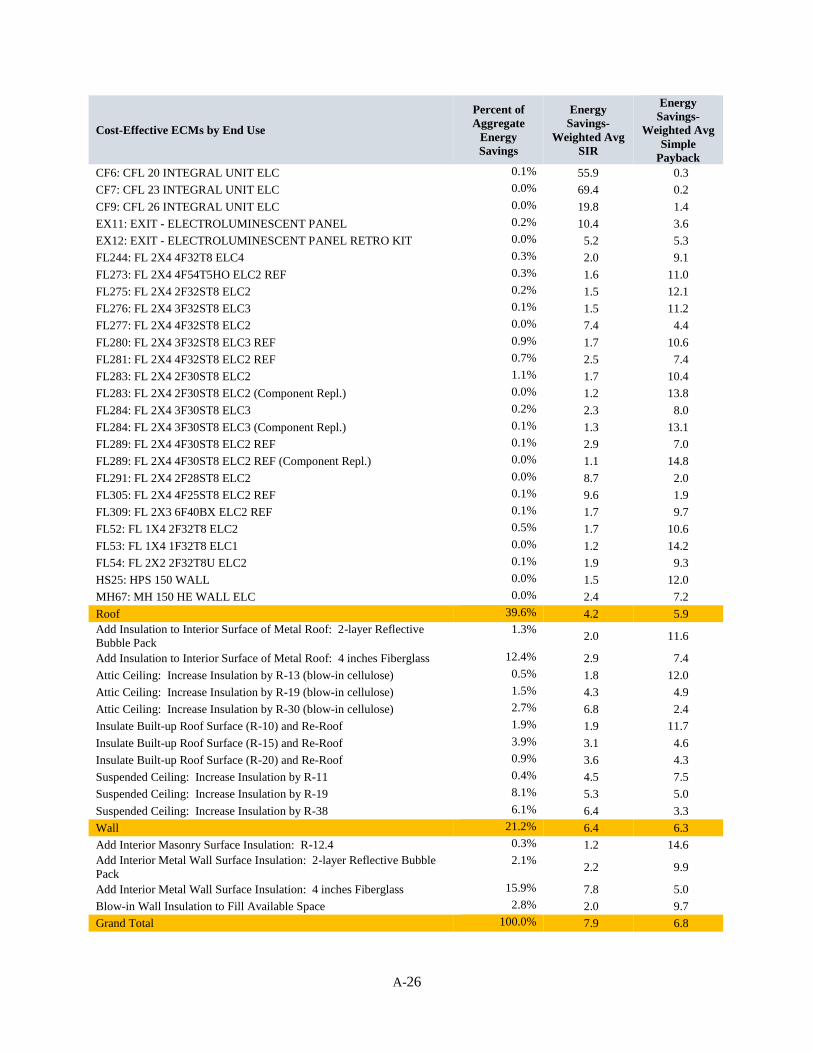
A-26
Cost-Effective ECMs by End Use
Percent of
Aggregate
Energy
Savings
Energy
Savings-
Weighted Avg
SIR
Energy
Savings-
Weighted Avg
Simple
Payback
CF6: CFL 20 INTEGRAL UNIT ELC 0.1% 55.9 0.3
CF7: CFL 23 INTEGRAL UNIT ELC 0.0% 69.4 0.2
CF9: CFL 26 INTEGRAL UNIT ELC 0.0% 19.8 1.4
EX11: EXIT - ELECTROLUMINESCENT PANEL 0.2% 10.4 3.6
EX12: EXIT - ELECTROLUMINESCENT PANEL RETRO KIT 0.0% 5.2 5.3
FL244: FL 2X4 4F32T8 ELC4 0.3% 2.0 9.1
FL273: FL 2X4 4F54T5HO ELC2 REF 0.3% 1.6 11.0
FL275: FL 2X4 2F32ST8 ELC2 0.2% 1.5 12.1
FL276: FL 2X4 3F32ST8 ELC3 0.1% 1.5 11.2
FL277: FL 2X4 4F32ST8 ELC2 0.0% 7.4 4.4
FL280: FL 2X4 3F32ST8 ELC3 REF 0.9% 1.7 10.6
FL281: FL 2X4 4F32ST8 ELC2 REF 0.7% 2.5 7.4
FL283: FL 2X4 2F30ST8 ELC2 1.1% 1.7 10.4
FL283: FL 2X4 2F30ST8 ELC2 (Component Repl.) 0.0% 1.2 13.8
FL284: FL 2X4 3F30ST8 ELC3 0.2% 2.3 8.0
FL284: FL 2X4 3F30ST8 ELC3 (Component Repl.) 0.1% 1.3 13.1
FL289: FL 2X4 4F30ST8 ELC2 REF 0.1% 2.9 7.0
FL289: FL 2X4 4F30ST8 ELC2 REF (Component Repl.) 0.0% 1.1 14.8
FL291: FL 2X4 2F28ST8 ELC2 0.0% 8.7 2.0
FL305: FL 2X4 4F25ST8 ELC2 REF 0.1% 9.6 1.9
FL309: FL 2X3 6F40BX ELC2 REF 0.1% 1.7 9.7
FL52: FL 1X4 2F32T8 ELC2 0.5% 1.7 10.6
FL53: FL 1X4 1F32T8 ELC1 0.0% 1.2 14.2
FL54: FL 2X2 2F32T8U ELC2 0.1% 1.9 9.3
HS25: HPS 150 WALL 0.0% 1.5 12.0
MH67: MH 150 HE WALL ELC 0.0% 2.4 7.2
Roof 39.6% 4.2 5.9
Add Insulation to Interior Surface of Metal Roof: 2-layer Reflective
Bubble Pack
1.3% 2.0 11.6
Add Insulation to Interior Surface of Metal Roof: 4 inches Fiberglass 12.4% 2.9 7.4
Attic Ceiling: Increase Insulation by R-13 (blow-in cellulose) 0.5% 1.8 12.0
Attic Ceiling: Increase Insulation by R-19 (blow-in cellulose) 1.5% 4.3 4.9
Attic Ceiling: Increase Insulation by R-30 (blow-in cellulose) 2.7% 6.8 2.4
Insulate Built-up Roof Surface (R-10) and Re-Roof 1.9% 1.9 11.7
Insulate Built-up Roof Surface (R-15) and Re-Roof 3.9% 3.1 4.6
Insulate Built-up Roof Surface (R-20) and Re-Roof 0.9% 3.6 4.3
Suspended Ceiling: Increase Insulation by R-11 0.4% 4.5 7.5
Suspended Ceiling: Increase Insulation by R-19 8.1% 5.3 5.0
Suspended Ceiling: Increase Insulation by R-38 6.1% 6.4 3.3
Wall 21.2% 6.4 6.3
Add Interior Masonry Surface Insulation: R-12.4 0.3% 1.2 14.6
Add Interior Metal Wall Surface Insulation: 2-layer Reflective Bubble
Pack
2.1% 2.2 9.9
Add Interior Metal Wall Surface Insulation: 4 inches Fiberglass 15.9% 7.8 5.0
Blow-in Wall Insulation to Fill Available Space 2.8% 2.0 9.7
Grand Total 100.0% 7.9 6.8

B-1
Appendix B. Estimating Impact of New Construction on the
2025 Federal Energy Goal: Detailed Methodology
The current method used to track improvements in building energy efficiency by federal agencies
relies on an aggregate energy use intensity (EUI) as means of measuring progress. The EUI is developed
for the total floor space of all buildings maintained by an agency, with the exclusion of some buildings
with distinctly abnormally high process loads. There is no distinction made for buildings of different
vintages.
This method thus incorporates the energy use and floor space of buildings that are constructed during
the period established for meeting the EUI reduction targets. It is clear then that newly constructed
buildings, built using the latest energy-efficient technologies and practices, will lower the overall EUI of
the stock of buildings, irrespective of actions taken by the agency to reduce the energy use in older
buildings. Given this situation, the setting of future goals with regard to the reduction of the stock EUI
must attempt to take into account the impact that new buildings might exert on the reduction in the EUI
for the stock of buildings.
An estimate of the impact of new building construction on any future EUI must consider two major
factors: 1) the percentage of new building floor space in the stock at the end of the goal-setting period,
and 2) the average difference of the EUI new buildings relative to the existing stock at the beginning of
the goal-setting period. For the current study, the projections pertain to the share and average intensity of
newly constructed federal building floor space over the period 2016-2025.
To develop values for these factors, considerable effort was devoted to understand how recently
constructed buildings may have influenced the progress that has been made from 2003. Having
approximate values of both the quantity and energy intensity of the floor space in buildings built over the
last decade would help inform any method to extrapolate the impact from this source out to 2025.
Unfortunately, the available data sources to estimate recently-built federal construction and the associated
overall energy intensity were inadequate for this task. Ideally, agencies reporting floor space and energy
efficiency data to the General Services Administration (GSA) and the Federal Energy Management
Program (FEMP) would include building characteristics such as year built, utilization (e.g., occupant
density and weekly hours), and location. This information would aid in determining how these newly
constructed buildings have influenced the historical evolution of agency-level EUIs. However, data with
this level of detail is not available.
With regard to simply estimating the magnitude of new (recently built) federal building floor space,
the available information sources outside the agencies reporting to GSA and FEMP are also inadequate.
This study examined new construction data provided by the McGraw-Hill Construction (MHC) company
and by the U.S. Census Bureau. Neither of these sources can be relied upon to develop a robust estimate
of recently built building floor space in the federal sector. A more complete discussion of what data are
available from all sources is contained in Appendix C.

B-2
The inadequacy of the data sources to provide direct estimates of recently constructed federal floor
area and associated energy intensity led to the development of alternative methods that rely heavily on
analyst judgment, but use empirical data where it is available.
These alternative methods are laid out in the following two subsections. Section B.1 presents a
method to project new federal construction between 2016 and 2025. The method relies primarily on an
estimate of how much floor space is disposed in each year (dependent in some degree on the reporting to
GSA as part of the Federal Real Property Profile, FRPP), and a projection of expected annual growth in
the stock of floor space.19
These values are established separately for each of the major agencies. Section
B.2 lays out the methodology to estimate the relative difference in the EUI for future federal buildings
(over the period 2016 to 2025) and the stock of federal buildings as of 2015. This methodology relies
heavily on recent analysis of the evolution of nonresidential building energy efficiency standards since
2004. These building energy efficiency standards form the basis of how much energy efficiency new
federal buildings will be required to incorporate over the coming decade.
B.1 Projected New Federal Construction, 2016-2025
There is considerable uncertainty as to the growth of the federal building stock out to 2025 given
continuing budget constraints and efforts to more effective utilize existing assets. To address this
question the research team considered separately the amount of floor area that might be replaced (due to
demolition, sale, or transfer) as well as the annual growth of floor area that may be required to meet the
agency’s mission. With regard to amount of replacement square footage, some guidance is provided in the
historical reporting to GSA as part of the FRPP.
The first two columns in Table B.1 present the average annual “disposals” of floor space over two
recent time periods, 2007-2012, and 2011-2012.20
The third column reflects a judgment as to average
annual disposals that might occur out through the year 2025. Using this assumption and an assumed
growth rate in total stock (the second shaded column), the simple stock accounting model yields an
approximate estimate of the amount of new (2016-2025) floor space that would be part of the stock at the
end of 2025 (shown in the last column of the table).
The agencies are grouped into three categories: 1) civilian agencies reporting through the FRPP, 2)
the U.S. Postal Service, USPS (whose floor space is reported to FEMP), and the 3) the Department of
Defense (DOD). The entries for DOD are based on the magnitude of floor space reported by means of its
Base Structure Report, which was provided by the Office of the Secretary.21
The table reflects a provisional scenario. In early July 2013, FEMP requested agencies to comment
on the disposal or growth assumptions pertaining to their particular agency.22
The highlighted portions of
the table represent analyst judgment. The darker highlighted entries identify agencies in which specific
19
The publicly available reports related to the FRPP can be found on GSA website:
http://www.gsa.gov/portal/category/21275 20
These data were based upon special tabulations, in spreadsheets, prepared by GSA for FEMP and transmitted to
PNNL via personal communication from FEMP’s Chris Tremper on May 10, 2013. These tables showing floor
space stock and disposals are shown as Appendix Tables B.1 and B.2. 21
The DOD magnitudes were obtained via personal communication from Ariel Castillo of the DOD, via a
spreadsheet sent to FEMP on September 4, 2013. 22
The FEMP request was sent as a series of email messages to appropriate agency staff on July 9, 2013.

B-3
responses to this request were obtained.23
With regard to the civilian buildings covered by the FRPP, the
average growth rate between 2015 and 2025 is projected to be 0.9 percent per year, just slightly higher
than the projected rate of population growth by the Census Bureau.24
Table B.1. Projected new 2016-2025 federal construction and share of 2025 stock (million square feet)
Notes:
1) Shaded cells represent assumed values by PNNL. Darker shaded cells reflect specific input from an agency.
2) USPS floor space is not reported to GSA as part of the FRPP, but is reported to FEMP.
Annual values of new construction and disposals from DOD were given for the years 2015 to 2020.
(See Table B.2.)25
The projections for new construction provided are based upon 5-year budget
projections. New construction floor space is projected to be 11.1 million square feet in 2016, 11.7 million
square feet in 2017, and 9.5 million square feet in 2018. However, the projected construction drops off
abruptly for 2019 and 2020 (0.7 million square feet in 2019 and 0.2 million square feet in 2020). These
lower most likely represent periods beyond the planning period for most elements in DOD, and would not
represent generally expected construction levels for these years. For the analysis here, it is assumed that
construction over the 2019-2020 averages just 8 million square feet per year. As a result, the level of
2,210 million square feet for 2020 is about 15 million square feet greater than the projection provided by
DOD for that year.
Table B.2. Projected floor space for the Department of Defense (military bases)
23
The response from the DOE was obtained via e-mail from Drew Campbell to Chris Tremper on July 18, 2013. 24
The 2012 Census Bureau projection (Series NP2012-T1) showed an annual growth rate in U.S. resident
population of 0.75% between 2015 and 2025. See Census Bureau website:
http://www.census.gov/population/projections/data/national/2012/summarytables.html 25
The darker shaded entries for the 2015 stock and 2016-2020 disposals are those supplied by DOD. The lighter
shaded reflect adjusted values from the DOD material.
Floor Space Growth Rate Floor Space Total Sq.Ft. % of 2025
2007-2012 2011-2012 2016-2025 2012 2012-2025 2025 (2016-2025) Stock
Civilian (FRPP) 8 20 13 1,205 0.9% 1,319 219 16.6%
Energy 1.4 4.2 1.5 117 0.3% 122 19 15.3%
GSA 3.3 10.0 5.0 417 0.8% 463 85 18.5%
Justice 0.1 0.3 0.3 71 0.8% 79 9 11.4%
VA 0.4 0.4 0.4 163 1.2% 182 18 9.9%
Agriculture 0.7 1.2 1.0 58 0.5% 62 13 21.1%
Home. Security 0.7 0.9 0.8 48 0.8% 53 12 22.7%
Interior 0.7 1.3 1.0 71 0.5% 76 14 18.0%
NASA 0.3 0.4 0.3 47 0.0% 49 5 10.9%
All Other 2.7 212 0.9% 233 44 18.7%
USPS (see Note) Not Avail. 0.4 273 -0.2% 265 4 1.5%
Dept. of Defense 4.7 2,300 2,240 98 4.4%
Average Disposals/Year
2015 2020 2025 2016-2020 2021-2025
Additions as %
of 2025 stock
Floor Space Stock 2,188 2,210 2,240 4.4%
New Construction 48.3 50
Disposals 26.6 20
B-4
No information was provided for the years beyond 2020. For these years, it was assumed that the
total construction would be similar to the previous five years, and that disposals would be somewhat
smaller (owing the greater prevalence of new floor space--that built after 2000). The net increase of 30
million square feet over this period is reflected in the projected 2025 floor space of 2,240 million square
feet.
Under these assumptions, these post-2015 additions would represent about 4.4 percent of the 2025
stock, as shown in the last column of Table B.2. Key entries from Table B.2 have been included in the
last row of the preceding table, B.1. The DOD also reported floor area for 2012, based upon the Base
Structure Report to be about 2,300 million square feet.
Calibration to floor space reported to FEMP under the goal-setting process
The values of floor space shown in Tables B.1 and B.2 are not based upon the magnitudes of floor
space reported to FEMP under the energy intensity goal setting process. For purposes of projecting future
floor area, the better and more transparent approach was deemed to employ the FRPP and Base Structure
Report values. However, for purposes of guiding the development of future energy intensity goals, the
most reasonable starting point is to adapt the floor space estimates that have been provided to FEMP.
It is assumed that the ratios of floor space reported to FEMP, as compared to floor space reported in
other contexts (e.g., FRPP, and DOD Base Structure Report), will remain constant in the future. Thus, as
a simple calibration procedure, a set of scaling factors was computed on the basis of the reported floor
space for 2012. It should be noted that under this assumption, the fractions of 2016-2025 new floor space
in the 2025 stock will be the same as those shown in the last column of Table B.1. However, for
aggregations (across the civilian agencies) the calculated values may differ as the distribution of floor
space by agency is different under the FEMP reporting as compared to the FRPP.
Table B.3 illustrates this calibration procedure and development of these scaling factors. The first
column shows the 2012 floor space reported to GSA under the FRPP for the civilian agencies (domestic
floor area only), the floor space reported to FEMP for the USPS, or the DOD floor space reported as part
of the Base Structure Report. The next two columns show the floor space reported to FEMP for 2012, the
first column showing only goal-subject floor space and the second column adding in the goal-excluded
floor space.
The last two columns show the respective ratios of FEMP reported floor space to the floor space
totals shown in column one. Scale-1 relates to goal-subject floor space and Scale-2 relates to the total
floor space reported to FEMP. Clearly, the largest deviation from 1.0 in the last column is associated
with GSA. Presumably, a large portion of leased space is not covered by the FEMP goal-setting
process.26
26
For the Veterans Administration (VA), the reason for larger amount of floor space reported to FEMP as compared
to the FRPP was not investigated. The scope of VA floor space as reported under the FRPP differs from that used
for reporting to FEMP.
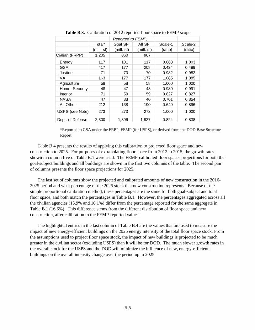
B-5
Table B.3. Calibration of 2012 reported floor space to FEMP scope
*Reported to GSA under the FRPP, FEMP (for USPS), or derived from the DOD Base Structure
Report
Table B.4 presents the results of applying this calibration to projected floor space and new
construction to 2025. For purposes of extrapolating floor space from 2012 to 2015, the growth rates
shown in column five of Table B.1 were used. The FEMP-calibrated floor spaces projections for both the
goal-subject buildings and all buildings are shown in the first two columns of the table. The second pair
of columns presents the floor space projections for 2025.
The last set of columns show the projected and calibrated amounts of new construction in the 2016-
2025 period and what percentage of the 2025 stock that new construction represents. Because of the
simple proportional calibration method, these percentages are the same for both goal-subject and total
floor space, and both match the percentages in Table B.1. However, the percentages aggregated across all
the civilian agencies (15.9% and 16.1%) differ from the percentage reported for the same aggregate in
Table B.1 (16.6%). This difference stems from the different distribution of floor space and new
construction, after calibration to the FEMP-reported values.
The highlighted entries in the last column of Table B.4 are the values that are used to measure the
impact of new energy-efficient buildings on the 2025 energy intensity of the total floor space stock. From
the assumptions used to project floor space stock, the impact of new buildings is projected to be much
greater in the civilian sector (excluding USPS) than it will be for DOD. The much slower growth rates in
the overall stock for the USPS and the DOD will minimize the influence of new, energy-efficient,
buildings on the overall intensity change over the period up to 2025.
Total* Goal SF All SF Scale-1 Scale-2
(mill. sf) (mill. sf) (mill. sf) (ratio) (ratio)
Civilian (FRPP) 1,205 860 967
Energy 117 101 117 0.868 1.003
GSA 417 177 208 0.424 0.499
Justice 71 70 70 0.982 0.982
VA 163 177 177 1.085 1.085
Agriculture 58 58 58 1.000 1.000
Home. Security 48 47 48 0.980 0.991
Interior 71 59 59 0.827 0.827
NASA 47 33 40 0.701 0.854
All Other 212 138 190 0.649 0.896
USPS (see Note) 273 273 273 1.000 1.000
Dept. of Defense 2,300 1,896 1,927 0.824 0.838
Reported to FEMP,

B-6
Table B.4. FEMP-calibrated floor space projections and new construction for goal-subject square
footage and total square footage
B.2. New Building Efficiency
This section discusses the methodology that was used to assess the reductions in EUI that would
likely be related to new, more efficient federal buildings constructed over the period 2016-2025. For this
element, the basic approach is to estimate the sources of the overall difference between the EUI in new
buildings (built between 2016 and 2025) and the EUI that will reflect the 2015 stock.
The basic approach first involves an assessment of the various influences or sources that may affect
the relative energy intensity of new versus existing buildings. These various sources are represented by
the first four columns in Table B.2. The fundamental quantification of changes in the average EUI is
based upon simulation analysis of prototypical buildings compliant with the American Society of
Heating, Refrigerating, and Air-Conditioning Engineers (ASHRAE) Standard 90.1-2004 (ASHRAE
2004) and ASHRAE Standard 90.1-2010 (ASHRAE 2010).
Table B.5. Impact on 2025 stock EUI from new construction meeting federal standard based
upon ASHRAE Standard 90.1-2010
Goal Sq.Ft. % of 2025 Total Sq.Ft. % of 2025
Goal SF All SF Goal SF All SF (2016-2025) Goal SF (2016-2025) Total SF
Civilian (FRPP) 880 989 940 1,056 149.0 15.9% 169.7 16.1%
Energy 102 118 106 122 16.1 15.3% 18.6 15.3%
GSA 181 213 196 231 36.2 18.5% 42.6 18.5%
Justice 72 72 78 78 8.9 11.4% 8.9 11.4%
VA 183 183 197 197 19.5 9.9% 19.5 9.9%
Agriculture 59 59 62 62 13.0 21.1% 13.0 21.1%
Home. Security 48 49 52 53 11.8 22.7% 12.0 22.7%
Interior 60 60 63 63 11.3 18.0% 11.3 18.0%
NASA 33 40 35 42 3.8 10.9% 4.6 10.9%
All Other 142 196 151 209 28.3 18.7% 39.1 18.7%
USPS 271 271 265 265 4.0 1.5% 4.0 1.5%
Dept. of Defense 1,804 1,833 1,847 1,877 81.0 4.4% 82.3 4.4%
All Federal 2,955 3,093 3,051 3,198 234.0 7.7% 256.0 8.0%
All Federal Civilian 1,151 1,260 1,205 1,321 153.0 12.7% 174 13.1%
2015 2025
Cumulative Additions Cumulative Additions
Design Design As Built
90.1-2004
relative to stock
-- improvement
90.1-2010
relative to 90.1-
2004
Federal Design
over relevant
standard
Takeback
from greater
intensity,
plug loads
Average EUI
compared to
2015 Stock
(% Reduction) (% Reduction) (% Reduction) (% Increase) (% Reduction
Low 5% 21% 5% 20% 11%
High 15% 26% 25% 10% 56%
Best Judgment 10% 24% 10% 15% 29%

B-7
The approach does not attempt to quantify absolute levels of energy intensity. While simulation
studies do generate such estimates, a standard caveat in such studies is that the EUIs represent ideal
operating conditions and assumed levels of electrical plug loads and typical operating schedules. For this
analysis, it is sufficient to assume that changes in actual EUI’s, from one energy standard to another, are
approximately proportional to changes in simulated EUIs that conform to the building energy efficiency
codes that reflect such standards.
The estimation process begins with an assumption as to how the energy intensity of buildings built to
the 90.1-2004 standard compare to that of the existing stock as of 2015. As shown in column one of
Table B.5, the “best judgment” estimate is that, on balance, federal buildings built to meet the 90.1-2004
standard are roughly 10% more energy efficient than the average stock of buildings with the further
assumption of a roughly comparable mix of building types.
One way of rationalizing this assumption is to rely on a recent DOE-sponsored study that sought to
quantify the overall energy intensity of “existing” buildings, as compared to “new” buildings. In early
2011, DOE issued a report entitled U.S. Department of Energy Commercial Reference Building Models of
the National Building Stock (DOE 2011). This report was the result of a collaborative effort among three
national laboratories: National Renewable Energy Laboratory, PNNL, and Lawrence Berkeley National
Laboratory. The report sought to represent three broad vintages of nonresidential buildings: “new”,
“post-1980”, and “pre-1980”. Different ASHRAE standards were used to characterize the energy-related
features of the buildings in these vintages. As indicated in the report, “The new construction models
comply with the minimum requirements of ANSI/ASHRAE/IESNA27
Standard 90.1-2004 (ASHRAE
2004), the post-1980 models meet the minimum requirements of Standard 90.1-1989 (ASHRAE 1990),
and the pre-1980 models are built to a set of requirements developed from previous standards and other
studies of construction practices.” While the pre-1980 buildings are not assigned a specific ASHRAE
standard, the lighting efficiencies were assumed to have been updated to be equivalent to the requirements
under Standard 90.1-1989.
More recent work at PNNL has developed estimates of the overall changes in overall commercial
intensity that are implied between 1989 ASHRAE standard and the 2004 standard. According to a
pending PNNL report that has developed estimates of historical benefits of building energy codes, the
overall reduction in the site energy intensity of newly constructed buildings meeting codes based on the
ASHRAE Standard 90.1 is about 16 percent between 90.1-1989 and 90.1-2004.28
The majority of this
change—approximately a 13 percent change—is between the ASHRAE standard published in 1999 (90.1-
1999) and that published in 2004. Thus, assuming that fewer buildings were built in the period 2000
(assumed to be earliest impact of the 1999 standard) as compared to the prior decade, the overall or
average change in the energy intensity in all buildings built between 1989 and 2004 would be something
less than 10 percent.
To the question of the current energy intensity of federal buildings prior to the 1989 standard, there is
little empirical basis to develop quantitative estimates. According to the same PNNL report cited above,
the change between the first edition of national building standards published by ASHRAE (Standard 90A-
1975 [ASHRAE 1975] and 90A-1980 [ASHRAE 1980]) and Standard 90.1-1989 was in range of 15
27
American National Standards Institute (ANSI) and Illuminating Engineering Society of North America (IESNA) 28
Livingston, OV, PC Cole, DB Elliott, and R. Bartlett. 2013. “Building Energy Codes Program: National Benefits
Assessment 1992-2040.” PNNL-22610 (pending).

B-8
percent. However, as noted above, the lighting efficacies these older buildings cited in the inter-
laboratory report on reference buildings were assumed to have achieved a level equivalent to the 1989
standard. Moreover, it is these older building where one can presume that much of the effort of federal
building energy managers have been targeted to achieve the intensity goals that are the subject of this
report. Thus, it is clearly inappropriate to rely strictly on the estimated changes in the ASHRAE
standards as a guide to the relative differences in energy intensity among different vintages of federally-
constructed buildings.
Given these considerations, the basic judgment employed in this analysis was that the energy intensity
of the current stock of federal buildings is approximately 10 percent higher than that implied by
compliance with the ASHRAE Standard 90.1-2004. This value is shown in the third row of the first
column of Table B.5. As also shown in the table, lower and upper bounds to this assumption are 5
percent and 15 percent.
Change between ASHRAE Standard 90.1-2004 and Standard 90.1-2010
The second step was to intuit the difference between Standard 90.1-2004 and Standard 90.1-2010. A
quantitative estimate of this difference is based upon another recent PNNL report that focused on this
same topic (Thornton et al. 2011). Using energy simulation analysis applied to16 prototypical
commercial buildings, this report estimated an overall reduction of about 23.2 percent in terms of site
energy intensity and 25.6 percent in terms of a metric based on energy cost. “Overall” reduction is
defined in terms of an estimated national distribution of all recent construction by building type. Also to
be noted is that these reductions consider the impact of including process and plug loads as part of the
building energy intensities.
One natural question is whether the composition of federal construction by building type is
sufficiently different from the composition of privately-owned buildings as to significantly alter these
calculated national average reductions. To explore this issue the percentage changes in energy intensities
by specific prototypical building were reweighted to reflect the composition of federal buildings. Ideally,
the composition of recently built federal buildings by floor area would be used in this reweighting.
Unfortunately, such data are not available. As proxy, the distribution of overall floor area by building
type at the end of FY 2012 was employed. The data for this distribution were based on a special
tabulation of the FRPP database that was developed for FEMP.29
Each of 19 separate building types from
the FRPP was associated with a prototypical building used in the PNNL study.
For the reduction in energy intensity, site energy was used for each prototypical building. The
reweighting based upon the composition of federal buildings turned out to make little difference to
calculated change in the overall energy intensity. Using the building type weights associated with the
2012 federal stock yielded an average change of 24.6 percent, about a one percentage point change from
the national average changes based upon composition of all (recently constructed) commercial buildings.
For purpose of this analysis, this figure was rounded down to 24 percent.30
29
Spreadsheets developed by GSA for FEMP and transmitted to PNNL via personal communication from FEMP’s
Chris Tremper on May 10, 2013. 30
The same calculation was also performed separately for the FY 2012 stock of civilian and military (Navy, Army,
and Air Force) floor space with representing. Somewhat surprisingly, the calculated percentage reduction in
intensity was somewhat greater for the military subset of federal buildings (25.1%), as compared to the total across

B-9
Requirement to exceed the ASHRAE 90.1 Standard
The third column in Table B.5 deals with the requirement that federal agencies design new buildings
to significantly exceed the requirements of the ASHRAE Standard 90.1 in terms of energy efficiency.
This requirement was first imposed in the 2005 Energy Policy Act (EPAct 2005). This legislation calls
for newly constructed federal buildings to achieved 30 percent energy savings relative to the most
recently published ASHRAE Standard 90.1. The 30 percent target, however, is contingent on the
additional energy efficiency design features to be cost effective.
This requirement became effective on January 3, 2007, as it applied to then prevailing ASHRAE
Standard 90.1-2004. The baseline standard was updated to Standard 90.1-2007 starting August 10, 2012.
According to the pending report on historical code benefits cited earlier, the overall reduction in energy
intensity from 90.1-2007 was about 5 percent compared to Standard 90.1-2004.31
FEMP has required
agencies to indicate their success in achieving the 30 percent target reduction relative to Standard 90.1.
From data supplied to FEMP on a building-by-building, many agencies reported that their designs of new
buildings have been able to meet this requirement. However, there is no supporting documentation or
empirical data that corroborates these declarations.
In July 2013, DOE issued an undated federal building efficiency standard based upon Standard 90.1.
The provisions of EPAct 2005 continue in place, thus continuing to require designs that achieve an
additional 30 percent savings if cost effective. With energy standard for new federal building
construction based on Standard 90.1-2010 going into effect on July 9, 2014, achieving this additional
improvement, a full 30 percent, is going to be more challenging. Because there is as yet no experience
with regard to compliance with this updated federal standard, this analysis has taken a conservative
position. The average improvement beyond Standard 90.1-2010 is assumed to be 10 percent. However, it
must be noted that there is considerable uncertainty related to this assumption, given that very few
buildings (public or private) have been designed to achieve this implied level of energy efficiency. In
Table B.5, the confidence bounds for this EPACT-mandated requirement are deemed to be as low as 5
percent and as high as 25 percent in terms of the percentage reduction below Standard 90.1-2010.
all civilian agencies (23.9%). While the site intensity reduction provided in the PNNL study for high-rise residential
buildings was lower than the “national average”, 12.3% vs. 25.6%, (assumed to apply to FRPP categories “family
housing” and “dormitories”) and where the proportion of such buildings is higher in the military services as
compared to the civilian stock, other factors offset this downward influence on the overall intensity reduction from
these residential buildings. For example, the proportion of educational buildings in the military stock was greater
than in the civilian stock, and estimated change in the energy intensity between 90.1-2004 and 90.1-2010 of these
buildings was relatively high (36%). The overall conclusion is that the differences in the composition of buildings
between the military and civilian sector in this case is not sufficiently high as to warrant independent analysis.
However, a caveat is that these distributions are based on the current stock and not on any projected distribution of
future federal construction in these two broad sectors. 31
This discussion starts with ASHRAE Standard 90.1-2004 rather than Standard 90.1-2007 because the most
detailed recent analyses of energy efficiency changes in various standards have employed 90.1-2004 as a key
reference point. If, assuming the estimated 5% improvement between Standard 90.1-2004 and Standard 90.1-2007
were applied to Table B.5, the percentage reduction in the first column (“best judgment”) would change from 10%
to 15%. Corresponding to this change would be a reduction in the improvement to subsequent move to a federal
standard based on Standard 90.1-2010. Thus, the difference would be result in a revision from the current figure of
24% to 19% in the second column of the table. Overall, these changes would have no net impact on the overall
influence of new buildings built to Standard 90.1-2010.

B-10
Effect of Utilization and Occupancy in New Buildings
The final factor considered in the analysis works in an opposing fashion to the previously discussed
factors. There is strong reason to believe that new commercial buildings in general have greater energy
intensity than the existing stock, a fact based simply on the notion that new buildings have higher
utilization (e.g., hours of operation per week) and are more densely occupied. Moreover, it is reasonable
to assume that plug loads and computer networks (including servers) are more prevalent in new buildings
than in existing buildings.
With regard to utilization among all commercial buildings, the 2003 CBECS indicated that median
weekly hours for buildings built after 1990 were about 8 percent greater than the median for all
buildings.32
From this same source, one finds that for buildings built between 1990 and 1999, the median
occupant density was about 3 percent greater than the stock of all (non-mall) buildings.33
Unfortunately,
there are no separately published data on these metrics for federally-owned buildings, although any such
values based upon the CBECS would likely be suspect owing to the small sample of federal buildings in
the overall survey. The basic position in the study here is that there would be differences in utilization
and occupant density in new federal buildings that would tend to increase their energy intensity relative to
older federal buildings, a roughly similar situation as that observed in the entire building stock.
With regard to the intensity of plug loads and computer-related equipment, there are no available data
that definitively point to the difference between the very newest buildings and the existing stock. The
closest measure that might reflect this characteristic from the 2003 CBECS is the total floor space of
buildings that contain a “separate computer area.” Across all (non-mall) commercial buildings the
percentage of total floor space for buildings with such a dedicated area and built between 2000 and 2003
was about 45 percent. For all buildings (across all vintages), the corresponding average was 41 percent.
Note that these values do not relate to the actual percentage of the total area devoted to computers, nor is
there any indication of the relative energy intensiveness of the computer installations themselves.
Nevertheless, the data are suggestive that computer-related electricity use is likely greater in newly
constructed buildings, and there is no reason not to assume that this situation does not also pertain to
federal buildings.
Taking into account these two considerations, the analysis here assumes that these factors might
offset the increases in design efficiency by an average 15 percent. As shown in Table B.5, the uncertainty
bounds for this value are set to restrict the range of this value to be between 10 percent and 20 percent.
Impact of Future Increases in New Building Energy Efficiency
The estimated impact on the 2025 stock EUI shown in Table B.5 is predicated on unchanging
requirements for new federal building construction, those related to ASHRAE Standard 90.1-2010. As
evident from the previous discussion, over the past decade ASHRAE has published new editions of
Standard 90.1on a consistent three-year cycle. Thus, over the next decade one may confidently predict
32
Energy Information Administration, 2003 CBECS: Building Characteristics Tables: Table B.2. Summary Table:
Totals and Medians of Floor space, Number of Workers, and Hours of Operation for Non-Mall Buildings.
Downloaded from EIA CBECS website: http://www.eia.gov/consumption/commercial/data/2003/pdf/b2.pdf 33
The median employment density for the most recently-constructed buildings in the 2003 CBECS (2000-2003) was
lower than the median for all vintages, but this value presumably reflects the fact that the very newest buildings
would have not yet achieved their design occupancy.
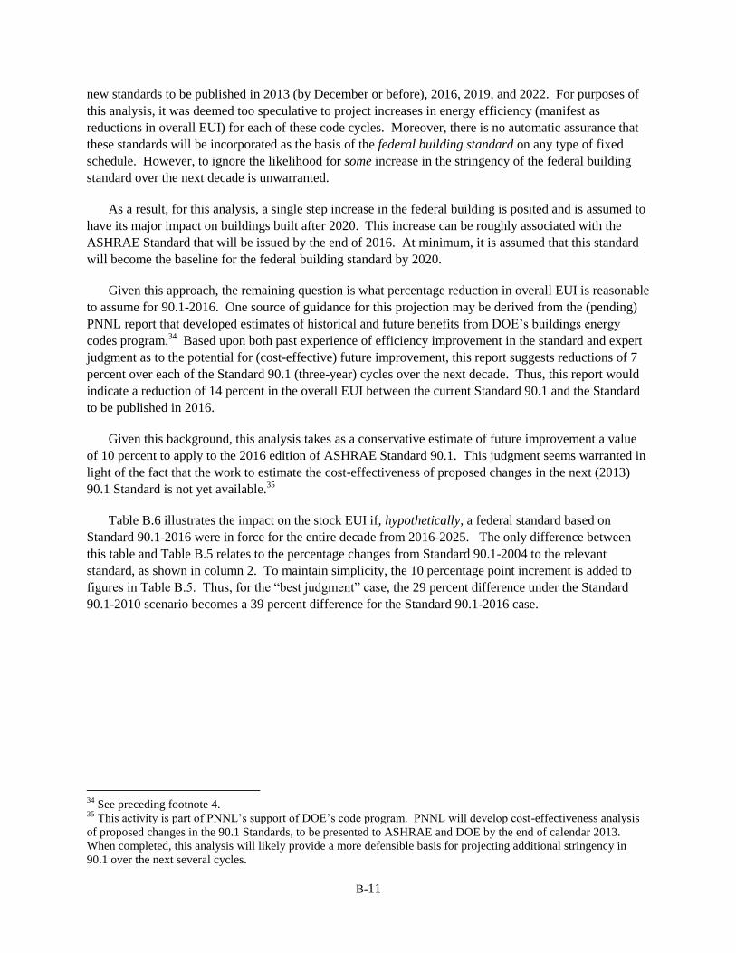
B-11
new standards to be published in 2013 (by December or before), 2016, 2019, and 2022. For purposes of
this analysis, it was deemed too speculative to project increases in energy efficiency (manifest as
reductions in overall EUI) for each of these code cycles. Moreover, there is no automatic assurance that
these standards will be incorporated as the basis of the federal building standard on any type of fixed
schedule. However, to ignore the likelihood for some increase in the stringency of the federal building
standard over the next decade is unwarranted.
As a result, for this analysis, a single step increase in the federal building is posited and is assumed to
have its major impact on buildings built after 2020. This increase can be roughly associated with the
ASHRAE Standard that will be issued by the end of 2016. At minimum, it is assumed that this standard
will become the baseline for the federal building standard by 2020.
Given this approach, the remaining question is what percentage reduction in overall EUI is reasonable
to assume for 90.1-2016. One source of guidance for this projection may be derived from the (pending)
PNNL report that developed estimates of historical and future benefits from DOE’s buildings energy
codes program.34
Based upon both past experience of efficiency improvement in the standard and expert
judgment as to the potential for (cost-effective) future improvement, this report suggests reductions of 7
percent over each of the Standard 90.1 (three-year) cycles over the next decade. Thus, this report would
indicate a reduction of 14 percent in the overall EUI between the current Standard 90.1 and the Standard
to be published in 2016.
Given this background, this analysis takes as a conservative estimate of future improvement a value
of 10 percent to apply to the 2016 edition of ASHRAE Standard 90.1. This judgment seems warranted in
light of the fact that the work to estimate the cost-effectiveness of proposed changes in the next (2013)
90.1 Standard is not yet available.35
Table B.6 illustrates the impact on the stock EUI if, hypothetically, a federal standard based on
Standard 90.1-2016 were in force for the entire decade from 2016-2025. The only difference between
this table and Table B.5 relates to the percentage changes from Standard 90.1-2004 to the relevant
standard, as shown in column 2. To maintain simplicity, the 10 percentage point increment is added to
figures in Table B.5. Thus, for the “best judgment” case, the 29 percent difference under the Standard
90.1-2010 scenario becomes a 39 percent difference for the Standard 90.1-2016 case.
34
See preceding footnote 4. 35
This activity is part of PNNL’s support of DOE’s code program. PNNL will develop cost-effectiveness analysis
of proposed changes in the 90.1 Standards, to be presented to ASHRAE and DOE by the end of calendar 2013.
When completed, this analysis will likely provide a more defensible basis for projecting additional stringency in
90.1 over the next several cycles.

B-12
Table B.6. Impact on 2025 stock EUI from new construction meeting federal standard based upon a
hypothetical ASHRAE Standard 90.1-2016
The final step involved estimating the impact that new building construction has on the average EUI
of the 2025 federal building stock. First, the relative amount of floor space built under the two efficiency
standards discussed above was established. It was assumed that half of the new floor space constructed
between 2016 and 2025 is effectively built to meet the baseline ASHRAE Standard 90.1-2010 and the
other half meets the more stringent ASHRAE Standard 90.1-2016. The average reduction in EUI is then
assumed to be 34 percent (i.e., an average of values in the highlighted cells in the last columns of Table
10).
The average expected reduction in EUI was then applied to the 13.1 percent of all newly constructed
floor space that civilian federal agencies were estimated to add to their building stock by 2015 (see “All
Civilian” in
Design Design As Built
90.1-2004
relative to stock
-- improvement
90.1-2016
relative to 90.1-
2004
Federal Design
over relevant
standard
Takeback
from greater
intensity,
plug loads
Average EUI
compared to
2015 Stock
(% Reduction) (% Reduction) (% Reduction) (% Increase) (% Reduction
Low 5% 25% 5% 20% 15%
High 15% 40% 25% 10% 70%
Best Judgment 10% 34% 10% 15% 39%
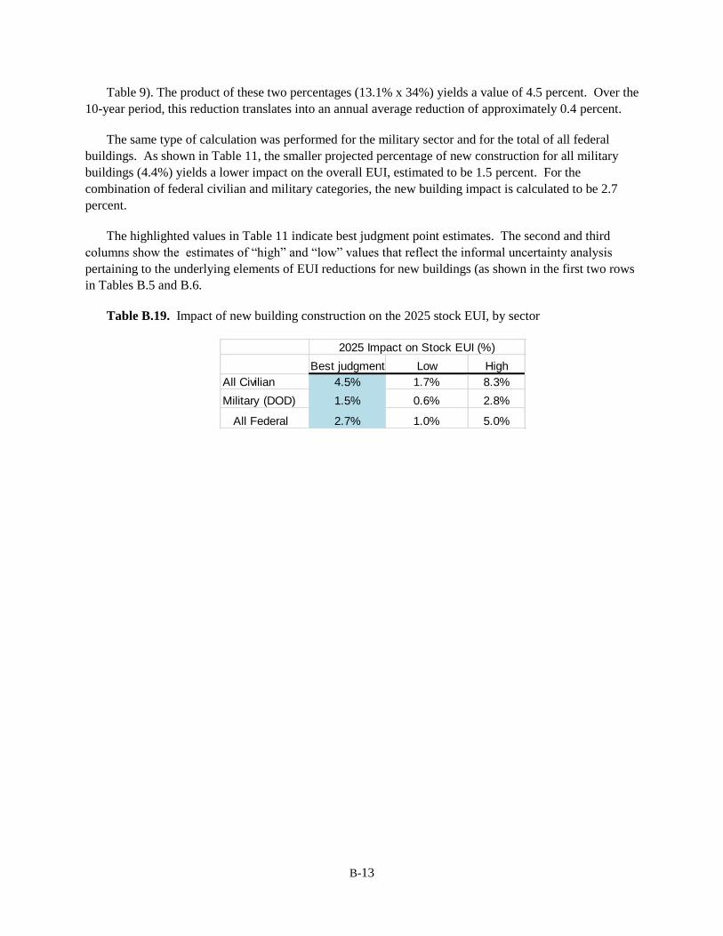
B-13
Table 9). The product of these two percentages (13.1% x 34%) yields a value of 4.5 percent. Over the
10-year period, this reduction translates into an annual average reduction of approximately 0.4 percent.
The same type of calculation was performed for the military sector and for the total of all federal
buildings. As shown in Table 11, the smaller projected percentage of new construction for all military
buildings (4.4%) yields a lower impact on the overall EUI, estimated to be 1.5 percent. For the
combination of federal civilian and military categories, the new building impact is calculated to be 2.7
percent.
The highlighted values in Table 11 indicate best judgment point estimates. The second and third
columns show the estimates of “high” and “low” values that reflect the informal uncertainty analysis
pertaining to the underlying elements of EUI reductions for new buildings (as shown in the first two rows
in Tables B.5 and B.6.
Table B.19. Impact of new building construction on the 2025 stock EUI, by sector
Best judgment Low High
All Civilian 4.5% 1.7% 8.3%
Military (DOD) 1.5% 0.6% 2.8%
All Federal 2.7% 1.0% 5.0%
2025 Impact on Stock EUI (%)

C-1
Appendix C. Data Sources to Estimate Recent Additions of
Federal Floor Space
To assess the potential impact of new federal construction on the overall EUI of future floor stock
maintained by the federal government, an effort was made estimate the amount floor space in recently
constructed federal buildings. Several data sources were examined in this effort, as described briefly in
the following sections.
C.1 McGraw-Hill Construction—F.W. Dodge
Unfortunately, there are no publicly available data sources that report annual new floor space of
commercial buildings and by ownership class (private, federal, state, local). Building project-level data
from the F.W. Dodge group of McGraw-Hill Construction (MHC) covering nonresidential building
projects over the period 2003 through 2010, have been used to support the development of nonresidential
building energy codes. They provide a basis for allocating the amount of construction by geographic and
climate zones across the U.S.
The project-level records available from Dodge show the type of building, value, floor space, type of
owner (private + 3 classes of public buildings listed above), and location (at the county level).
MHC/Dodge has collected this data for many decades; it is primarily used as a means of disseminating
building specifications for proposed new buildings to facilitate the construction solicitation and bid
process. The data pertain to the new building contracts and the timing of the data is based upon the award
of such contracts, not on the subsequent construction activity or project completion. As such, the
MHC/Dodge data differ as to their timing as compared to the construction estimates published by the U.S.
Census Bureau. The Census Bureau attempts to estimate the actual amount of construction activity
(measured in dollars) by month.
Table C.1 is based on aggregation of buildings shown as being built under federal ownership from the
MHC/Dodge project-level data. The amount of construction activity funded by federal agencies and the
branches of the military increased dramatically over the last years of the previous decade. The square
footage associated with construction contracts more than doubled between the 2005-2006 period and the
2008-2009 period.36
Because MHC/Dodge only has a single category for all federally-owned buildings, there is no
definitive way to discriminate between military and civilian construction. The numbers shown in Table
C.1 for military are the sum of two building classifications by Dodge: 1) Armories/Military Buildings
and 2) Dormitories. It is reasonable to expect that the majority of dormitories reported by MHC/Dodge
pertain to military housing. In each year over the 2005-2009 interval, these two categories showed the
two largest amounts of floor space. Moreover, it must be noted that these estimates likely understate
actual military construction because some portion of offices, “food/beverage service” buildings, stores,
and schools were also built on military bases.
36
The 2010 data were transmitted to PNNL in a separate data file, and were not integrated into the analysis here.
There is a question as to whether the level of 2010 federal construction may have been influenced by federal
stimulus that was initiated in 2009.
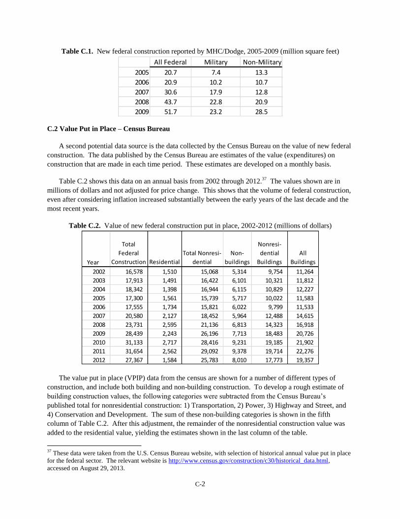
C-2
Table C.1. New federal construction reported by MHC/Dodge, 2005-2009 (million square feet)
C.2 Value Put in Place – Census Bureau
A second potential data source is the data collected by the Census Bureau on the value of new federal
construction. The data published by the Census Bureau are estimates of the value (expenditures) on
construction that are made in each time period. These estimates are developed on a monthly basis.
Table C.2 shows this data on an annual basis from 2002 through 2012.37
The values shown are in
millions of dollars and not adjusted for price change. This shows that the volume of federal construction,
even after considering inflation increased substantially between the early years of the last decade and the
most recent years.
Table C.2. Value of new federal construction put in place, 2002-2012 (millions of dollars)
The value put in place (VPIP) data from the census are shown for a number of different types of
construction, and include both building and non-building construction. To develop a rough estimate of
building construction values, the following categories were subtracted from the Census Bureau’s
published total for nonresidential construction: 1) Transportation, 2) Power, 3) Highway and Street, and
4) Conservation and Development. The sum of these non-building categories is shown in the fifth
column of Table C.2. After this adjustment, the remainder of the nonresidential construction value was
added to the residential value, yielding the estimates shown in the last column of the table.
37
These data were taken from the U.S. Census Bureau website, with selection of historical annual value put in place
for the federal sector. The relevant website is http://www.census.gov/construction/c30/historical_data.html,
accessed on August 29, 2013.
All Federal Military Non-Military
2005 20.7 7.4 13.3
2006 20.9 10.2 10.7
2007 30.6 17.9 12.8
2008 43.7 22.8 20.9
2009 51.7 23.2 28.5
Year
Total
Federal
Construction Residential
Total Nonresi-
dential
Non-
buildings
Nonresi-
dential
Buildings
All
Buildings
2002 16,578 1,510 15,068 5,314 9,754 11,264
2003 17,913 1,491 16,422 6,101 10,321 11,812
2004 18,342 1,398 16,944 6,115 10,829 12,227
2005 17,300 1,561 15,739 5,717 10,022 11,583
2006 17,555 1,734 15,821 6,022 9,799 11,533
2007 20,580 2,127 18,452 5,964 12,488 14,615
2008 23,731 2,595 21,136 6,813 14,323 16,918
2009 28,439 2,243 26,196 7,713 18,483 20,726
2010 31,133 2,717 28,416 9,231 19,185 21,902
2011 31,654 2,562 29,092 9,378 19,714 22,276
2012 27,367 1,584 25,783 8,010 17,773 19,357

C-3
Comparison with MHC/Dodge Data
To assess whether the VPIP estimates can be used to make an approximate estimates of newly-
constructed federal floor space, it is necessary to compare the VPIP numbers with those available from
MHC/Dodge over a comparable time period. For this comparison it assumed that there is generally a one-
year lag between the contract values reported by Dodge and the actual construction expenditures reflected
in VPIP data. In part, this assumption is based on the generally larger types of building projects
undertaken for the federal government as compared to private construction.
Using this assumption, the value of MHC/Dodge value of construction projects over the five-year
period 2005 through 2009 was 36.0 billion dollars. From Table C.2, over the five-year period 2006
through 2010, total VPIP for federal construction activity was 85.7 billion dollars.
This difference suggests that a significant share of federal construction may not be included in the
MHC/Dodge database. Projects in agencies that undertake construction by their employees or use
alternative methods to disseminate requests for bids would not find their way into the Dodge database.
From other PNNL work to support the DOE’s activities related to commercial building energy codes,
it is known that the MHC/Dodge database does not cover all projects in the private sector as well. In
developing its VPIP data for the private nonresidential construction in the U.S. the data from
MHC/Dodge is adjusted up by 25 percent to account for under-coverage of projects.38
Moreover, in terms
of comparing value estimates, the MHC/Dodge data do not includes some important cost elements,
including site preparation, architectural and engineering (A&E) fees, and other miscellaneous costs. To
compare the VPIP and MHC/Dodge data for the private sector over the same (five) years as above, the
equivalent calculations yield a total of 999.6 billion dollars for VPIP and 610.4 billion dollars for
MHC/Dodge.
If the ratios between estimated for VPIP and the Dodge/MHC contract value are compared over the
five-year periods, the calculated ratio is 1.64 for the private sector, and 2.37 for the federal sector. The
difference in these two ratios is likely accounted for by both greater under-coverage of MHC/Dodge for
federal sector projects and higher architectural and engineering costs that one could expect to be
associated with federal projects. Unfortunately, there is no publicly available information to distinguish
between these factors.39
A very rough method to adjust MHC/Dodge estimates is used to estimate recent floor space additions.
Several key assumptions are required, however. This begins with the estimates for the private sector.
Using the published factor of 1.25 to represent under-coverage by MHC, then a second factor to account
for additional cost elements (e.g., Architectural and Engineering [A&E] fees) would be 1.31 (1.64/1.25).
Next, it is assumed that the A&E costs for federal construction are, on average, twice as high as for
38
See the methodology description on http://www.census.gov/const/www/methodpage.html. 39
This situation was confirmed in a discussion with a Census Bureau staff member responsible for the federal VPIP
estimates. As noted in the Census Bureau documentation, the volume of construction activity in the federal sector is
less reliant on MHC/Dodge as in the private sector, and involves collecting information directly from many federal
agencies. Thus, there is no constant adjustment factor (e.g., the 25% alluded to above) to account for under-
coverage by MHC/Dodge. Due to confidentiality the Census Bureau is unable to release information that would
identify the difference between MHC/Dodge data and the overall estimate of federal construction expenditure over
any given time period. Source: personal communication with Rachel Hammond, Manufacturing and Construction
Division, U.S. Bureau of the Census, June 13, 2013.

C-4
typical private nonresidential construction. With this assumption the approximate level of under-
coverage for federal construction for this particular time period is backed out. That step involves dividing
1.62 (1 + 2 x 0.31) into the overall VPIP/(MHC) ratio of 2.37, which yields a value of about 1.5. Thus,
on the basis of this highly simplified analysis, the MHC/Dodge value of construction represented about
two-thirds of all federal construction over this period.
Before considering how to translate this result into an estimate of floor space in recently built federal
buildings, one additional aspect of the VPIP data should be noted. The VPIP estimates include
expenditures for both new buildings and renovations of existing buildings. According to the Census
Bureau, no effort has ever been made to distinguish these two types of construction as part of the VPIP
methodology.40
The MHC/Dodge database does distinguish between these types of construction.
However, for the analysis here, these two categories for federal expenditures were not broken out
separately, helping to make the comparisons between the MHC/Dodge and VPIP data consistent in terms
of scope.
C.3 Federal Real Property Profile Database
The third potential source of information concerning floor space built and maintained by the federal
government are data collected by the General Service Administration’s Office of Government-wide
Policy (GSA/OGP). Data on the number of buildings and structures and building square footage by
agency have been published annually since 2002 in publication entitled the “Federal Real Property Report
(FRPR),”41
which are based on the FRPP database.
The FRPR includes a table of the number of disposed assets during the preceding fiscal year.
However, as published, this table shows only the disposed assets rolled up across the entire federal
government. Moreover, only the number of disposed building are shown, and not the associated floor
space.
As part of a special request from the FEMP to GSA/OGP to support this project, two spreadsheets
were prepared that showed total floor space by agency and the total amount disposed square footage for
each fiscal year between 2006 and 2012.42
The intent of this request was to determine if information on
the amount of total floor space in different years, combined with disposals of floor space, could be used to
estimates the amount of new floor space added over particular time intervals.
In order the smooth out year-to-year fluctuations in the amount of disposed floor area, the analysis
focused on the beginning (2006) and ending years (2012) of the supplied FRPP data. If the data on
dispositions and floor space stock were internally consistent, then the additions to floor space (new
40
See previous footnote. 41
All of these reports can be found on the GSA website: http://www.gsa.gov/portal/content/102880. The data prior
to 2005 was collected somewhat differently than the more recent data, and so comparability across all categories of
assets is not available. As of June 2013, the latest report included on this website is for FY 2010. 42
These data were based upon special tabulations, summarized in two separate spreadsheets, prepared by the GSA
for FEMP and transmitted to PNNL via personal communication from FEMP’s Chris Tremper on May 10, 2013.
The relevant file names are: 1) FRPP FY 2006 2011tremper non disposed by agency use legal interest.xlsx, and 2)
FRPP FY 2006 2011tremper disposed by agency use legal interest.xlsx.

C-5
construction + newly leased space) between 2006 and 2012 could be estimated as the difference between
the stocks in those years plus the disposed assets over the 2007 through 2012 period.43
Before examining the reported data in detail, it should be noted that the floor space numbers provided
by GSA/OGP in this request do not include the amount of square footage outside U.S. states and
territories. In the last available FRPR for fiscal year (FY) 2010, the total reported square footage was
3.402 billion. In the data provided for this analysis, the total square footage for FY 2010 was 2.922
billion. This difference is accounted for primarily by military facilities overseas, as well as State
Department buildings.44
Table C.3 shows the results of the calculation procedure used to infer additions to floor space. The
first two columns of the table show the total floor space by agency reported for 2006 and 2012. A perusal
down these two columns indicates that there is not uniform reporting across all agencies in the FRPP.
Nine agencies reporting square footage in 2012 did not report in 2006; however, the floor space
represented by these agencies is relatively small.
The third column in the table shows the calculated amount of disposals summed over the fiscal years
2007 through 2012. The uneven pattern of disposals is reflected in the notes in right-most column of the
tables. However, generally years in which no disposals are reported relate to the relatively small
agencies, and so it would not be unexpected that no buildings would have been disposed in a single year
or over a short period of consecutive years.
The last column shows the implied additions over this six-year period, based upon the reported stock
and disposal values however caution should be applied in interpreting the implied additions from this
procedure. For five agencies, the implied additions are negative, clearly indicating inconsistencies in the
stock and disposal reporting over this period. This largest issue relates to the Navy where the reported
disposals are not sufficient to explain the large decline in the reported stock between 2006 and 2012.
The bottom rows in the table provide some aggregations of agency data. For the uniformed services,
the total of the implied additions is approximately 70 million square feet over this period. However, this
value is clearly too low, as it includes the implausible results for the Navy (negative additions). The last
two rows of the table attempt to develop an approximate estimate of new additions for the civilian
agencies as whole. In the second-to-last row, the sum is calculated for agencies in which the disposal data
was deemed to be credible (reporting all or most years, without significant gaps). Using this criterion,
total additions are estimated to have been in about 86 million square feet between 2006 and 2012 (built in
2007 or later). The last column excludes agencies where the implied additions were negative. Using this
additional criterion, the total increases to 96 million square feet (or about 16 million square feet per year).
In an effort to better understand some of the limitations of the FRPP data, particularly related to
disposals, some questions were directed at the staff member at GSA charged with assembling the
database.45
Among other issues, it was learned that the disposal values can be distorted by short-term
leases that are started and stopped within a fiscal year. A related issue in general is the treatment of the
43
The 2006 disposals would have occurred prior to reporting of the stock at the end of FY 2006. 44
The Department of State total shown in the 2010 FRPR was 74.1 million square feet, while the value reported via
this special extract was 1.7 million square feet (presumably primarily covering agency buildings in Washington,
D.C.). 45
Personal communication, via conference call, with Chris Coneeney of GSA on May 30, 2013.

C-6
expiration of leased buildings. Finally, it was acknowledged that agencies may have applied different
criteria over the years as how to classify active buildings as part of their stock.
With the notion that the reporting of both stock and disposals may have improved in the most recent
years, another processing of the FRPP was undertaken to include only the most recent two years. Table
C.3 shows the same information as Table C.2, but where the implied additions are estimated only for
2011 and 2012. In general, the numbers are more plausible. For only four agencies does the calculation
of implied additions imply a negative value. With regard to disposals, those agencies not reporting any
disposals are relatively small and thus reasonable to expect no disposals over a two-year period.
Unfortunately, as an aggregate estimate for the uniformed services, the implied additions cannot be
used, as the implied additions for the Army is negative. The Army has provided detailed information on
construction, and so reliance on the FRPP reporting is not necessary.
The last two rows of the table provide approximate estimates of the implied additions for 2011-2012
period for all civilian agencies. Similar to the discussion related to Table C.3, the estimate is performed
by first including and then excluding agencies where the implied additions are negative. In the latter case,
the results indicate that about 54 million square feet may have been added over this period. The implied
annual average of 27 million square feet is more than 50 percent greater than the 2007-2012 estimate
derived from Table C.3. This magnitude is likely influenced by some construction financed by the federal
economic stimulus program, but is probably a more accurate representation than that yielded by the
analysis of the 2006-2012 dataset. The longer data is more likely to less consistent in reporting practices
over time. Based upon the overall analysis, it appears reasonable to suggest that additions of new
construction of federal civilian agency buildings have ranged between 20 and 30 million square feet in
recent years.

C-7
Table C.3. Building floor space by agency for 2006 and 2012 and implied additions
Agency Square Feet (Thousands) Notes
Reported Reported 2007-2012 Implied
2006 Stock 2012 Stock Disposed Additions
Agriculture Total 59,477 57,779 4,350 2,652
Air Force Total 558,525 492,961 133,066 67,502
Army Total 790,574 738,104 79,165 26,695
Broadcasting Board of Governors Total 2 137 No disposals reported
Commerce Total 7,730 8,968 552 1,790
Commodity Futures Trading Commission Total 0 435 No disposals reported
Corps of Engineers Total 15,108 11,878 795 -2,434
Defense/WHS Total 7,751 8,269 77 595 Disposals only reported for 2012
DC Court Services & Offender Supervision Agency Total 0 348 No disposals reported
Energy Total 132,515 116,940 8,488 -7,087
Environmental Protection Agency Total 3,993 4,356 No disposals reported
Federal Communications Commission Total 0 112 Only 1 small building disposed, ignored
General Services Administration Total 384,409 420,545 20,032 56,168 No disposals reported for 2008-2010
Health and Human Services Total 32,713 34,538 2,406 4,232
Homeland Security Total 42,098 48,107 4,002 10,011
Independent Government Offices Total 135 0 No disposals reported
Interior Total 110,939 105,865 4,369 -705
John F. Kennedy Center for the Performing Arts Total 0 1,500 No disposals reported
Justice Total 68,379 71,424 716 3,760
Labor Total 20,545 25,042 516 5,013 No disposals reported for 2007, 2009-2010
Merit Systems Protection Board Total 0 8 Only 1 small building disposed, ignored
National Aeronautics And Space Administration Total 44,298 46,779 1,594 4,075
National Archives and Records Administration Total 4,475 5,292 No disposals reported
National Gallery of Art Total 0 1,420 No disposals reported
National Science Foundation Total 1,100 1,321 16 833 No disposals reported for 2007-2009
Navy Total 534,055 437,368 72,011 -24,676
Office of Personnel Management Total 91 81 No disposals reported
Smithsonian Total 0 11,866 222 No disposals reported for 2007-2008, 2010-2011
State Total 1,257 1,748 No disposals reported
State (USAID) Total 4 4 No disposals reported
Tennessee Valley Authority Total 4,315 27,883
Transportation Total 27,632 25,723 1,008 -901 No disposals reported for 2007-2010
Treasury Total 5,744 6,786 375 866
United States Holocaust Memorial Council Total 0 320 No disposals reported
Veterans Affairs Total 150,275 162,702 2,473 14,900
Grand Total 3,008,138 2,876,608 336,233 204,704
Grand Total, as published (used for check) 3,008,138 2,876,608
Uniform Services 1,883,153 1,668,432 284,242 69,521 Issue with negative implied additions for Navy
All other, reporting in both years 1,124,984 1,204,788
All other, reporting in both years, with credible disposal data 1,045,955 1,083,342 49,601 86,988
All other, reporting in both years, with credible disposal data, add. > 0 787,393 848,659 35,949 97,215

C-8
Table C.4. Building floor space by agency for 2011 and 2012 and implied additions
Agency Square Feet (Thousands) Notes
Reported Reported 2011-2012 Implied
2010 Stock 2012 Stock Disposed Additions
Agriculture Total 58,531 57,779 2,468 1,716
Air Force Total 499,635 492,961 37,336 30,661
Army Total 775,596 738,104 24,444 -13,048
Broadcasting Board of Governors Total 137 137 No disposals reported
Commerce Total 7,800 8,968 37 1,205
Commodity Futures Trading Commission Total 412 435 No disposals reported
Corps of Engineers Total 9,751 11,878 86 2,214
Defense/WHS Total 8,081 8,269 77 266 Disposals reported only for 2012
DC Court Services & Offender Supervision Agency Total 232 348 No disposals reported
Energy Total 129,000 116,940 8,488 -3,572
Environmental Protection Agency Total 4,293 4,356 No disposals reported
Federal Communications Commission Total 170 112 0.10 Only 1 small building disposed, ignored
General Services Administration Total 417,438 420,545 20,020 23,127
Health and Human Services Total 36,083 34,538 966 -579
Homeland Security Total 46,974 48,107 1,748 2,881
Independent Government Offices Total No disposals reported
Interior Total 102,995 105,865 2,548 5,419
John F. Kennedy Center for the Performing Arts Total 1,500 1,500 No disposals reported
Justice Total 70,053 71,424 564 1,934
Labor Total 24,942 25,042 448 548
Merit Systems Protection Board Total 59 8 Only 1 small building disposed, ignored
National Aeronautics And Space Administration Total 45,572 46,779 749 1,955
National Archives and Records Administration Total 5,270 5,292 No disposals reported
National Gallery of Art Total 1,425 1,420 No disposals reported
National Science Foundation Total 1,345 1,321 14 37
Navy Total 447,609 437,368 12,863 2,622
Office of Personnel Management Total 81 81 No disposals reported
Smithsonian Total 11,601 11,866 121 No disposals reported for 2011
State Total 1,660 1,748 No disposals reported
State (USAID) Total 4 4 No disposals reported
Tennessee Valley Authority Total 26,939 27,883
Transportation Total 27,851 25,723 1,008 -1,120
Treasury Total 6,128 6,786 318 406
United States Holocaust Memorial Council Total 320 320 No disposals reported
Veterans Affairs Total 153,255 162,702 879 10,327
Grand Total 2,922,743 2,876,608 115,184 69,050
Grand Total, as published (used for check) 2,922,743 2,876,608
Uniform Services 1,722,841 1,668,432 74,643 20,234 Issue with negative implied additions for Army
All other, reporting in both years 1,196,516 1,204,788 40,541 48,814
All other, reporting in both years, with credible disposal data 1,196,516 1,204,788 40,541 48,814
All other, reporting in both years, with credible disposal data, add. > 0 1,003,581 1,027,587 30,080 54,086
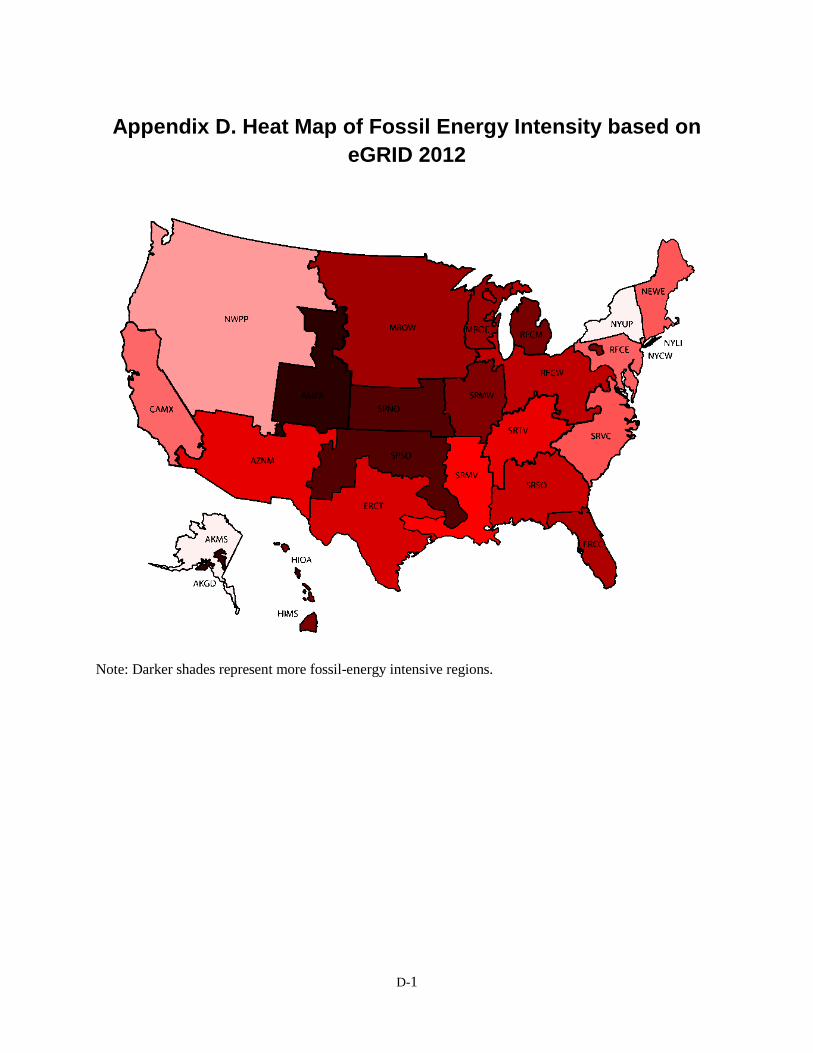
D-1
Appendix D. Heat Map of Fossil Energy Intensity based on
eGRID 2012
Note: Darker shades represent more fossil-energy intensive regions.
