analysis of different gray zone treatments in wrf-les real ... · (wrf) model (skamarock et al.,...

Analysis of Different Gray Zone Treatments in WRF-LES Real CaseSimulationsPaula Doubrawa1, Alex Montornès2, Rebecca J Barthelmie3, Sara C Pryor4, and Pau Casso2

1National Renewable Energy Laboratory, Golden, CO, USA2VORTEX, Barcelona, Spain3Sibley School of Mechanical and Aerospace Engineering, Cornell University, Ithaca, NY, USA4Earth and Atmospheric Sciences, Cornell University, Ithaca, NY, USA

Correspondence to: Paula Doubrawa ([email protected])

Abstract. When conducting meso-micro scale coupled atmospheric simulations, it is crucial to ensure an adequate treatment of

gray zone or terra incognita resolutions in which a large portion of the kinetic energy is naturally produced by the momentum

balance equations in the model, while the remaining part still needs to be parameterized. In this work, we conduct three multi-

day, real case, full-physics atmospheric simulations that are fully coupled from the meso to the micro scale and in which the

only difference is the treatment of boundary layer physics at the gray zone domain. One simulation uses a well-established5

parameterization, another uses its scale-aware version previously modified to accommodate gray zone resolutions, and a final

one uses no parameterization at all and assumes that the gray zone domain can be run in large-eddy simulation (LES) mode.

The simulated fields are cross-compared, and further compared to measurements collected during the Prince Edward Island

Wind Energy Experiment. Use of LES in the gray zone domain influences the flow fields in a manner that is robust to temporal

averaging. The best predictions of vertical wind shear were found for the simulations in which the gray zone is parameterized,10

and the inclusion of a micro scale nest run in LES mode within the gray zone domains increased the model errors by producing

overly homogeneous flow fields. The parameterized simulations also produced better agreement in terms of kinetic energy

spectra at the two innermost simulation domains. In the gray zone domain, the energy decays as f−3 throughout most of the

spectral range considered. In the micro scale domain, the same is only seen in the low-frequency end of the gray zone spectral

range. In the high-frequency end, the energy decay follows a f−1 slope. Outside the gray zone spectral range, the micro scale15

simulated spectra follow the expected f−5/3 slope and produce good agreement with measurements.

1 Introduction

Recent advances in computational resources and atmospheric models have been driving the wind energy research community

away from the Reynolds-Averaged Navier Stokes (RANS) approach, which does not permit a study of turbulence at the high

Reynolds numbers that characterize flow within wind farms. Instead, research is increasingly based on Large-Eddy Simulations20

(LES) in which the horizontal grid size (∆xy) of the mesh is reduced to a point where Navier Stokes can be assumed to resolve

all of the turbulence scales relevant to the problem at hand. However, due to their relatively high computational cost compared to

RANS-based codes, LES have traditionally been used to examine ideal cases where a large number of assumptions simplify the

1

Wind Energ. Sci. Discuss., https://doi.org/10.5194/wes-2017-61Manuscript under review for journal Wind Energ. Sci.Discussion started: 15 January 2018c© Author(s) 2018. CC BY 4.0 License.

problem sufficiently for computational tractability and physical understanding (e.g., Schalkwijk et al. (2015); Shin and Hong

(2013)). In this work, an important distinction is made between “idealized” and “real case” simulations based on the data being

used as initial and boundary conditions. In idealized simulations, the model is often driven towards specified values of wind

speed and temperature which are defined with the intent of representing canonical atmospheric conditions (e.g., Churchfield

et al. (2012)). In real case simulations, initial and boundary conditions are specified to match a past event of interest and often5

a reanalysis data set is used to drive the model.

Another important distinction relevant for this work is that between “full-physics” and “fluid dynamics” models. In addition

to focusing on idealized conditions, LES studies for wind farm aerodynamics have historically used fluid dynamics solvers that

do not include the full range of atmospheric physics and dynamics that impact flow within wind farms (e.g., cloud physics and

radiative processes). Thus far, full-physics real case LES focusing on atmospheric phenomena at micro scales have typically10

employed models that run un-coupled from the meso and macro scales (e.g., Kunz et al. (2000)) and for a time period on

the order of hours (e.g., Liu et al. (2012)). For the purpose of this work, we distinguish between macro, meso, and micro

atmospheric scales based on the duration (T ) and spatial dimensions (L) of the most energetic processes within them as given

in Table 1.

Table 1. Scales of atmospheric motions as defined for the present work based on duration and spatial dimension of most energetic processes

within them.

Duration Spatial Dimension

Macro Scale 1 year < T < 1 day 104 km < L< 101 km

Meso Scale 1 day < T < 1 hour 101 km < L< 100 km

Micro Scale T < 1 hour L < 1 km

Ongoing computational developments have only recently started to allow for full-physics, real case atmospheric simulations15

to be performed for wind energy applications. This can be achieved by coupling meso and micro scale models, and is a topic

of active research for which two main approaches are being considered. One alternative is to perform meso scale simulations

with an atmospheric model uncoupled from the micro scale and to subsequently use the meso scale flow to prescribe initial

and boundary conditions to a secondary code that is then run on a smaller domain, a finer mesh, and in LES mode. Another

alternative is to fully couple the meso and micro scales within a single code. As a consequence of these new developments,20

two important questions have emerged. Firstly, how best to prescribe initial and boundary conditions to the LES and whether

to allow feedback between the scales when the coupling is performed within a single code. Secondly, how best to treat the

transition from meso to micro scales within numerical models (Sanz Rodrigo et al., 2016). The concept of “gray zone” (GZ)

resolutions or “terra incognita” was coined to describe the spatial scales O(102− 103) m at which Navier Stokes is able to

resolve a substantial fraction of the kinetic energy in the atmospheric boundary layer (ABL), while still needing to model the25

remaining part with physical parameterizations (Wyngaard, 2004). Under the first coupling approach, the GZ is avoided but

turbulence generation methods must still be applied to the meso scale fields before they can be used as driving inflow to LES

2


(Haupt et al., 2015; Mirocha et al., 2013). Under the second coupling approach, an adequate treatment of GZ resolutions is

required and may be achieved by developing more flexible parameterizations (Shin and Dudhia, 2016; Ito et al., 2015) or by

avoiding the GZ domains altogether and relying on turbulence generation strategies alone to couple meso and micro scale

domains (Muñoz-Esparza et al., 2017).

A lot of the recent work in this field has focused on meso-micro coupling within the Weather Research and Forecasting5

(WRF) model (Skamarock et al., 2008), which is a widely used framework for idealized and real case meso scale atmospheric

simulations that can be run in LES mode by reducing ∆xy down to the micro scale and disabling several parameterizations.

For example, Shin and Hong (2015) and Ito et al. (2015) used idealized WRF-LES as benchmarks and developed scale-aware

capabilities within existing ABL parameterizations (ABLPs) to regulate their role at GZ resolutions. So far, these and other

ABLPs expanded to accommodate GZ resolutions are limited to convective boundary layers (CBLs) and have mostly been10

verified against reference idealized LES (e.g., Shin and Dudhia (2016); Ito et al. (2015); Kitamura (2015); Honnert et al.

(2011)). The only existing work evaluating meso-micro coupled simulations with WRF for a real case avoided the GZ by using

a high nesting ratio and going directly from the meso (1 km) to the micro scale (90 m) domain (Muñoz-Esparza et al., 2017).

While this approach provided satisfactory results when compared with observations over a diurnal cycle, it is still important to

continue the development of techniques to accurately simulate atmospheric flow at intermediate resolutions.15

Very little work has been done to understand how the simulated flow responds to different treatments of GZ resolutions

under real case LES that are fully coupled to the meso scale. Boutle et al. (2014) applied aircraft observations to evaluate

simulations of stratocumulus formation under the proposed scale-aware modifications to the Met Office Unified Model, while

nesting domains from 4 km to 100 m and considering a period of 2 days. They found that the performance of the scale-aware

ABLP at the GZ matched the performance of the well-established one-dimensional large-scale ABLP used for coarser grids,20

and that of the three-dimensional small-scale parameterization typically used for micro scale grid sizes. Another study by Shin

and Hong (2015) proposed a scale-aware ABLP in WRF and validated it for real cases considering 24 hours of observational

data focusing on the development of a convective roll at ∆xy = 333 m. They found that the newly proposed scheme enhanced

the simulation of vertical motions under convective conditions but highlighted the need for further improvements which will

cover a wider range of simulation scenarios. A different study was carried out by Schalkwijk et al. (2015), where the effect of25

modifications to the GALES model was assessed by comparing one year of simulation data at ∆xy = 100 m to observations

from a meteorological mast. They found that the best agreement of simulations with observations occurred for ABL parameters

that are explicitly resolved (i.e., instead of parameterized) thus further highlighting the need for long-term real case LES and

for further research in meso-micro scale model coupling.

More research is needed to guide future developments of scale-aware one-dimensional ABLPs that can reach down from the30

meso to the micro scale, and of three-dimensional ABLPs that can reach up from the micro to the meso scale. The research

presented herein addresses this need by evaluating different approaches for treating GZ resolutions in full-physics real case

LES of the atmosphere that are fully coupled to the meso scale. This is the first study in which real case WRF-LES simulations

are performed for a period longer than one day. Moreover, it is the first such study that focuses on quantifying the differences

in simulated flow arising from different GZ treatments. We focus on flow parameters of relevance to wind engineering and35

3


quantify differences between three simulations in which the GZ is treated differently by being run with a well-established

ABLP, its scale-aware version, and no ABLP at all. The simulation output is compared to observational data collected during

the Prince Edward Island Wind Energy Experiment (Barthelmie et al., 2016). This specific location was selected for our

analysis because the terrain complexity and roughness changes found at the site warrant the use of LES in contrast to coarser,

meso scale simulations which are unable to resolve the complex flow characteristics at the site. The analysis considers a 16-day5

period thus enabling an assessment of the simulations performance under a range of atmospheric conditions and several diurnal

cycles. The methodology is discussed in Section 2. A cross-comparison of the model simulations is given in Section 3, and a

comparison between the simulations and measurements in Section 4. A final discussion can be found in Section 5.

2 Methodology

2.1 Boundary Layer Treatment at the Gray Zone10

Parameterized phenomena in meso scale atmospheric models (such as WRF, when it is not run in LES mode) include radiative

transfer, convection, and ABL physics. In ABLPs, a distinction is made between local vertical transport between adjacent grid

levels and non-local vertical transport via strong updrafts that span the ABL depth (Frech and Mahrt, 1995). Non-local ABL

schemes such as the well-established YSU (Hong et al., 2006) include a non-local term in addition to the local transport. The

SH scheme (Shin and Hong, 2015) is an expansion of YSU in which the amount of SGS vertical transport that needs to be15

parameterized is regulated based on ∆xy and on the strength of the non-local transport itself.

All simulations presented herein use the YSU ABLP for domains with a grid resolution coarser than the GZ resolution, and

are run in LES mode for the innermost domain in which the grid resolution is finer than at the GZ. The WRF source code

was modified to enable meso-micro scale coupling based on the potential temperature perturbation method of Muñoz-Esparza

et al. (2014, 2015). Previous work has shown that this modification results in an improvement to simulations of wind speed20

and turbulence intensity under different meteorological regimes and terrain complexities (Montornès et al., 2016b, a).

Hereinafter, the three simulations conducted are referred to as YSU_LES, SH_LES, and LES_LES (Table 2) based on how

they handle the ABL physics at the GZ and at the innermost domain. In the LES_LES simulation, the ABLP is switched off

in the GZ domain and the SGS energy is modeled with a local closure in which a 1.5-order prognostic equation for turbulent

kinetic energy (TKE) is used. This approach is recommended when the energy-containing eddies are substantially larger than25

the grid resolution (Shin and Hong, 2015) which is not necessarily the case at the GZ. Therefore the GZ treatment in our

LES_LES simulation is not necessarily a physical choice, but can be justified by the existence of a nested domain which is

appropriately run in LES mode.

4


Table 2. Treatment of atmospheric boundary layer physics at each simulation domain for the three simulations conducted in the experiment.

Simulation Name

Atmospheric Boundary Layer Parameterization (ABLP)

Meso Scale Domains Gray Zone Domain Micro Scale Domain

∆xy = 9 km,3 km,1 km ∆xy = 333 m ∆xy = 111 m

YSU_LES YSU YSU None

SH_LES YSU SH None

LES_LES YSU None None

Because the differences between YSU and SH pertain to the strength of the vertical transport, we expect differences in

vertical flow velocities and in vertical fluxes of heat and momentum between these two simulations. In idealized simulations, the

system complexity is lower and substantial differences between YSU_LES and SH_LES are only expected during convective

conditions (i.e. strong non-local transport) while under neutral and stable stratification, SH should default to its underlying

YSU structure. On the other hand, the higher level of complexity in a real case simulation precludes the predetermination of5

the exact effects that SH will have on the results. This complexity further highlights the need for the present study in which

these differences are investigated. Prior to the analysis, the only claim that can be made for the real case simulations conducted

is that a distinction between YSU_LES and SH_LES is only expected during isolated periods throughout the simulation, when

the differences between YSU and SH are noticeable. Instead, the largest difference is expected to be found between LES_LES

and the other two simulations in which the ABL is parameterized.10

2.2 Study Domain and Measurements

The simulations were conducted for a domain centered on the North Cape of Prince Edward Island for the period of the Prince

Edward Island Wind Energy Experiment field campaign (Barthelmie et al., 2016) at the Wind Energy Institute of Canada in

May 2015. The narrow and flat island spans ∼ 2 km across the measurement site (Fig. 1). To the west, a 10-14 m escarpment

marks the transition from ocean to continent. An 80 m meteorological mast compliant with the International Electrotechnical15

Commission standards and equipped with 3D Gill Windmaster Pro sonic anemometers collected 10 Hz wind and temperature

measurements at the heights (z) 20, 40, and 60 m above ground. The mast location is ∼ 900 m (∼ 400 m) from the coast in the

north (west) direction.

The data from each sonic anemometer were subject to despiking, detrending and coordinate rotation when calculating vari-

ances and covariances. Data were further conditionally sampled to exclude wind directions associated with wind turbine wakes20

(unless otherwise noted in the analysis) and then used to compute streamwise, transverse, and vertical wind speeds, and vertical

fluxes of heat and momentum. Conditions during the experiment period were dominated by onshore flow over the escarpment

(SW-NW flow was observed 75% of hours) and the Obukhov length as computed from the sonic anemometers indicate unstable

conditions on ∼ 10% of hours, and stable conditions on ∼ 25− 30% of hours (Barthelmie et al., 2016).

5


#*

422000 422500 423000 423500 5208

000

5208

500

5209

000

5209

500

5210

000

±0 0.25 0.5km

Elevation [m]0 - 55 - 1010 - 1515 - 20

North

ing [m

]

Easting [m]

(a) Site satellite imagery and elevation.

(b) WRF simulation domains.

Figure 1. Measurement site terrain elevation, satellite imagery from Environmental Systems Research Institute, and location of meteorolog-

ical mast (triangle) (a). Simulation domains from ∆xy = 9 km to ∆xy = 111 m (b).

2.3 Simulations

We performed three simulations using the Advanced Research WRF core version 3.7.1 that differ only in their treatment of

the GZ domain as described in Section 2.1. A total of five domains (with 70 x 70 grid points) were configured, centered at the

meteorological mast location following a set of telescopic nests from 9 km to 111 m (Fig. 1b). Feedback between the scales is

disabled so that the GZ fields can be analyzed without any influence from the turbulence that develops at the innermost domain5

which is run in LES mode across all simulations. Fifty vertical levels are defined throughout the domain, which are distributed

every ∼ 10 m in the ABL and stretched in the free atmosphere. Initial and boundary conditions for all domains are taken from

the Climate Forecast System Reanalysis (Saha et al., 2010) at a spatial resolution of ∼ 38 km. Topography for the highest

resolution domain is taken from the Shuttle Radar Topography Mission (Jarvis et al., 2008) at a 90 m spatial resolution, and

land use from GlobCover (Bontemps et al., 2011) at a ∼300 m spatial resolution.10

The analysis of model output focuses on flow parameters in the ABL surface layer. The model was run for a 16-day period

and time series were saved exclusively for the grid point closest to the meteorological mast location (Fig. 1a) for seven heights

above ground between ∼ 10 m and ∼ 180 m. The model saves historic output with a temporal frequency of 4 Hz, which are

immediately used to compute 10 minute-averaged diagnostics.

2.4 Variables and notation15

All analyses are performed for a fixed location (i.e., the meteorological mast) and consider vertical profiles of 10-minute mean

quantities. Hereinafter, the overbar ( ) is used to denote 10-minute averages when referring to (co)variances, but is omitted for

all other variables to simplify the notation. We focus on flow variables of relevance to wind energy such as horizontal wind

6


speed, wind direction, vertical wind shear, and turbulence intensity. Turbulence intensity is only calculated for time stamps

in which the horizontal wind speed is ≥ 3 m s−1 which are most relevant to wind energy applications. While the focus of

this work is on variables of interest to wind energy, we also choose to include vertical flow velocities and vertical fluxes

of heat and momentum which are crucial to characterizing turbulence and atmospheric stability. Perturbations are calculated

by subtracting the 10-minute mean from the 4 Hz instantaneous values as the simulation output is produced, and then used5

to obtain turbulence diagnostics at a 10-minute frequency. The turbulence diagnostics computed are kinematic heat flux and

turbulent kinetic energy TKE = TKE∆ +TKESGS . TKE∆ represents the amount of TKE that is explicitly resolved by the

model at a grid resolution ∆xy including the ABLP budget, and TKESGS is the amount that is produced by the turbulence

closure model when no ABLP is used and the simulation is run in LES mode. The SGS partition is diagnosed by the model

directly, and the resolved partition is calculated as TKE∆ = 12

(u′2 + v′2 +w′2

).10

Differences in simulation output that arise from varying the model configuration are discussed in Section 3 without reference

to the measurements. To avoid selecting one of the three cases as the reference benchmark, these differences are quantified

by a deviation from each simulation to the ensemble average of the three simulations. The model performance relative to

observations is quantified in a similar fashion by subtracting the modeled fields from the measured values. To facilitate a later

comparison with measurements, the majority of the model cross-comparison section focuses on the measurement heights of15

20, 40, and 60 m by linearly interpolating from the model levels to the target height.

2.5 Spectral Analysis

Spectral methods are used to compare the kinetic energy content of each data set in the frequency domain. Comparisons are

presented between the three simulations, between the two innermost domains for each simulation, and between simulations and

measurements. The power spectral density (PSD) values are computed for time series of 10-minute mean wind speeds using20

the Welch method. Previous work considering onshore and offshore sites has found that wind speed measurements collected at

a frequency of 10 minutes are sufficient to accurately estimate the PSD in the atmospheric surface layer (Larsén et al., 2016).

Because the spectral analysis is based on relative comparisons between the data sets, it is not concerned with energy leakage

at low frequencies that could be caused by non-stationarity in the time series, and a hanning window with a length of 1 day

is applied when computing PSD values. With a temporal frequency of 10 minutes and a window length of 1 day, the spectra25

are limited to 1 day−1 < f < 20 min−1 which is sufficient when focusing on GZ phenomena. High frequency fluctuations

are therefore not included in the spectra, but are instead contained in the analysis of turbulence intensity and TKE which are

computed from the 4 Hz model output.

3 Cross-Comparison of Simulations

In this section the three simulations are cross-compared to quantify their sensitivity to different treatments of the ABL physics30

at the GZ scale. Section 3.1 focuses on horizontal and vertical wind speeds, Section 3.2 on vertical wind shear and turbulent

kinetic energy, and Section 3.3 discusses the energy content of each simulation in the frequency domain.

7


3.1 Horizontal and Vertical Flow

To compare the flow predictions across the three simulations, an ensemble average was first computed and then differences

between each simulation and this reference ensemble were obtained at each time step. The values given in Fig. 2 show the

mean and standard deviation of these differences at each hour of the day, including 16 days of simulation and 6 10-minute

values in each hour. On average, the LES_LES simulation produced higher values of horizontal wind speed U and of vertical5

velocities w than the parameterized simulations. For both wind speed and vertical flow, there is no clear tendency of the mean

differences with time of day. Rather, a consistent difference is seen that decreases with height for U and that remains of the

same magnitude for w across the three heights. As expected, differences between YSU_LES and SH_LES are intermittent and

average out when a long time series is considered. The standard deviation of these differences is also substantially larger for

LES_LES than for the other two simulations, indicating that running the GZ domain in LES mode produces more fluctuations10

in the solution than activating a traditional or scale-aware ABLP.

Figure 2. Differences between each simulation and their ensemble average for horizontal wind speed (top) and vertical flow velocity (bottom)

for the heights 20 m (left), 40 m (middle) and 60 m (right). Error bars give the mean ± standard deviation of differences at each hour of day.

Values are for the GZ domain.

When considering all model levels for which output was saved (Fig. 3), it is clear that LES_LES produces higher wind

speed estimates only in the lower portion of the profile, and that the opposite is true above ∼ 60 m. Mean differences across

the simulations for vertical flow decrease with height, while the standard deviation of these differences increases for the

8


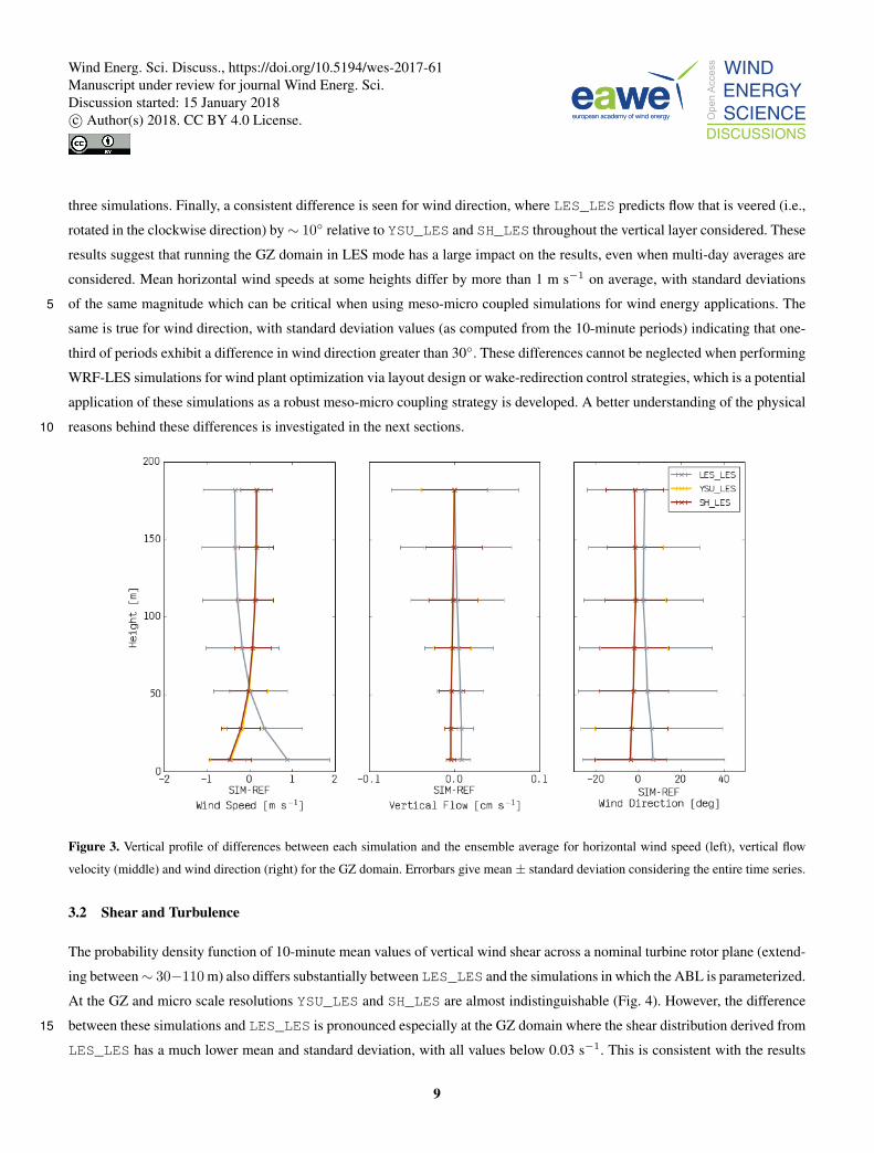
three simulations. Finally, a consistent difference is seen for wind direction, where LES_LES predicts flow that is veered (i.e.,

rotated in the clockwise direction) by∼ 10◦ relative to YSU_LES and SH_LES throughout the vertical layer considered. These

results suggest that running the GZ domain in LES mode has a large impact on the results, even when multi-day averages are

considered. Mean horizontal wind speeds at some heights differ by more than 1 m s−1 on average, with standard deviations

of the same magnitude which can be critical when using meso-micro coupled simulations for wind energy applications. The5

same is true for wind direction, with standard deviation values (as computed from the 10-minute periods) indicating that one-

third of periods exhibit a difference in wind direction greater than 30◦. These differences cannot be neglected when performing

WRF-LES simulations for wind plant optimization via layout design or wake-redirection control strategies, which is a potential

application of these simulations as a robust meso-micro coupling strategy is developed. A better understanding of the physical

reasons behind these differences is investigated in the next sections.10

Figure 3. Vertical profile of differences between each simulation and the ensemble average for horizontal wind speed (left), vertical flow

velocity (middle) and wind direction (right) for the GZ domain. Errorbars give mean± standard deviation considering the entire time series.

3.2 Shear and Turbulence

The probability density function of 10-minute mean values of vertical wind shear across a nominal turbine rotor plane (extend-

ing between∼ 30−110 m) also differs substantially between LES_LES and the simulations in which the ABL is parameterized.

At the GZ and micro scale resolutions YSU_LES and SH_LES are almost indistinguishable (Fig. 4). However, the difference

between these simulations and LES_LES is pronounced especially at the GZ domain where the shear distribution derived from15

LES_LES has a much lower mean and standard deviation, with all values below 0.03 s−1. This is consistent with the results

9


discussed in Section 3.1 which indicate higher vertical velocities for the LES_LES simulation, resulting in more homogeneous

flow and less vertical wind shear in the surface layer. This result is also evident in the micro scale domain, where the mean and

standard deviation of shear are still lower for LES_LES than for the other two simulations, evidence of the importance of the

ABL treatment at the GZ when conducting simulations with multiple nested domains.

Figure 4. Curve-fitted histograms for vertical wind shear between ∼ 30− 110 m, considering the 16 days of simulation. Values shown for

GZ and micro scale domains.

Fig. 5 shows the TKE budget from the three simulations for the highest measurement height (z = 60 m) and allows us to5

examine how the treatment of the ABL physics at the GZ resolution affects the total TKE budget within the two innermost

domains. At the GZ domain, differences between LES_LES and the two other simulations are obvious, and result from the fact

that LES_LES produces large amounts of subgrid TKE for wind speeds > 8 m s−1, while the other two produce none. When

TKESGS is combined with TKE∆ which is of the same magnitude for the three simulations, large differences result in the

total TKE budget between LES_LES and the other two simulations. High TKE at ∆xy = 333 m in LES_LES contributes to10

explaining the low vertical wind shear values seen in this simulation (Fig. 4).

In the micro scale nest, differences in TKE between LES_LES and the other two simulations are lower in magnitude but

still clearly noticeable. These differences are similar to those seen in the GZ domain, thus suggesting propagation down the

model chain. In the micro scale domain, these differences end up modulating the budget of SGS, modeled TKE and leading to

differences in TKESGS across the different simulations. While SH_LES and YSU_LES present median TKESGS values that15

increase with wind speed up to 15 m s−1, LES_LES shows a local TKE maximum between 10 and 12 m s−1 coinciding with

the peak of subgrid TKE production in the GZ domain when run in LES mode. These results suggest that the subgrid TKE

production at the GZ domain enabled by running it in LES mode inhibits the subgrid TKE production at the micro scale nest.

In other words, the use of ABLPs at the GZ results in lower TKE at the GZ domain but in higher TKE at the innermost nest.

10


0.0 0.2 0.4 0.6 0.8 1.0

Bin Center U [m s−1]

0.0

0.2

0.4

0.6

0.8

1.0

TKE

at z

= 6

0 m

[m2 s

−2]

0.0

0.1

0.2

∆xy = 333 m YSU ∆xy = 333 m SH ∆xy = 333 m LES

4 6 8 10 12 140.0

0.2

0.4

∆xy = 111 m

4 6 8 10 12 14

∆xy = 111 m

4 6 8 10 12 14

∆xy = 111 m

Figure 5. Median (markers) TKE at 60 m [m2 s−2] as a function of wind speed [m s−1] discretized in 1 m s−1 bins in the GZ (top) and

micro scale (bottom) domains. Solid lines delimiting shaded area give 25th and 75th percentile values.

3.3 Energy Spectra

The results presented in this section are based on the spectral analysis methods described in Section 2.5. The PSD for wind

speeds considering the entire 16-day time series are shown for the three simulations in Fig. 6. As expected, YSU_LES and

SH_LES exhibit higher PSD values when compared to LES_LES because the ABLP (enabled in YSU_LES and SH_LES)

acts to generate turbulence at length scales higher than the grid size. Note that this analysis is different from the one presented5

in Section 3.2 which encodes turbulence information frequencies up to 4 Hz. An important result from this spectral analysis is

that this difference between LES_LES and the other two simulations is seen throughout the spectrum, and is not concentrated

in the spectral tail as might be expected.

Fig. 6 also indicates that the energy decay at the GZ domain follows a f−3 slope instead of the f−5/3 expected for meso scale

and boundary layer turbulence at frequencies larger than 1 day−1 (Larsén et al., 2016). This result suggests that the GZ domain10

is lacking energy for the three simulations, and that a better treatment of turbulence at this scale is needed as will be further

discussed in Section 4.3. At the micro scale domain, the spectra are substantially more energetic at higher frequencies and

exhibit the f−1 decay seen in Muñoz-Esparza et al. (2017) for these frequencies, also exclusively in the nested LES domain.

Because simulation data are unavailable at temporal resolutions higher than 10 minutes, an in-depth analysis of the energy

content at higher frequencies is not possible and we cannot determine whether the expected spectral behavior is achieved for15

f > 20 min−1.

11


Figure 6. Power spectral density as a function of frequency for the 16-day time series of 10-minute mean horizontal wind speeds at z = 60

m for the three simulations at the GZ and micro scale domains.

4 Comparison of Simulations and Measurements

In this section the three simulations are compared to measurements from sonic anemometers to quantify how much improve-

ment can be gained from having a micro scale domain nested within a multi-scale simulation framework, and to determine

which GZ treatment produces the overall best results in terms of mean flow velocities and turbulence. Section 4.1 focuses on

horizontal wind speed, Section 4.2 on vertical wind shear and turbulent kinetic energy, and Section 4.3 compares the energy5

content of each data set in the frequency domain. Thus far the simulations have been cross-compared without reference to

the measurements to illustrate the sensitivity of flow parameters to different GZ treatments in each simulation. In this section,

we evaluate the simulated flow fields relative to the observational data set described in Section 2.2. Whenever not explicitly

specified, the comparison considers simulation data from the micro scale domain.

4.1 Horizontal Wind Speed10

Fig. 7 shows the distribution and magnitude of horizontal wind speed errors as a function of different atmospheric conditions

in terms of wind speed, wind direction, and turbulence intensity. An obvious and important result from this analysis is that

the YSU_LES and SH_LES error distribution is almost indistinguishable regardless of the atmospheric conditions considered,

indicating that the differences between these two simulations discussed in Section 3 are lower in magnitude than the model

error. The data distribution histogram above the leftmost subplot shows that most of the observed wind speeds are between 215

and 14 m s−1, and that wind speed errors exhibit a decreasing tendency with increasing wind speed. Although time stamps in

which the meteorological mast was subjected to a wind turbine wake were filtered out, the model still over-estimates the wind

12


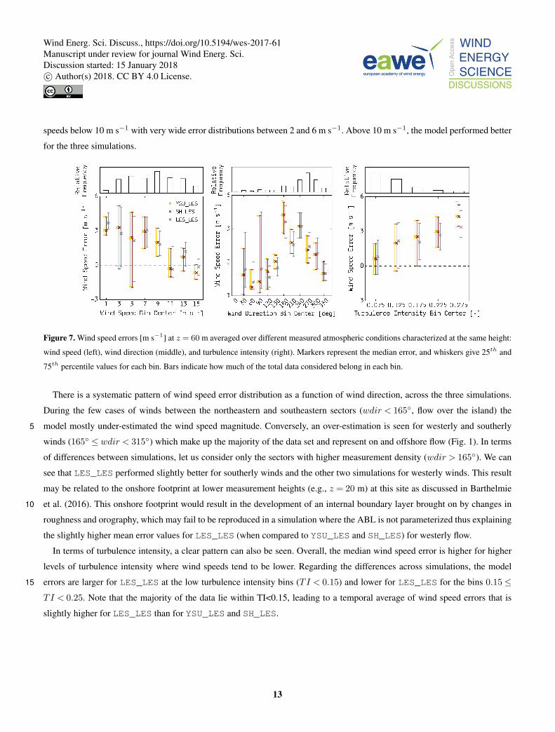
speeds below 10 m s−1 with very wide error distributions between 2 and 6 m s−1. Above 10 m s−1, the model performed better

for the three simulations.

Figure 7. Wind speed errors [m s−1] at z = 60 m averaged over different measured atmospheric conditions characterized at the same height:

wind speed (left), wind direction (middle), and turbulence intensity (right). Markers represent the median error, and whiskers give 25th and

75th percentile values for each bin. Bars indicate how much of the total data considered belong in each bin.

There is a systematic pattern of wind speed error distribution as a function of wind direction, across the three simulations.

During the few cases of winds between the northeastern and southeastern sectors (wdir < 165◦, flow over the island) the

model mostly under-estimated the wind speed magnitude. Conversely, an over-estimation is seen for westerly and southerly5

winds (165◦ ≤ wdir < 315◦) which make up the majority of the data set and represent on and offshore flow (Fig. 1). In terms

of differences between simulations, let us consider only the sectors with higher measurement density (wdir > 165◦). We can

see that LES_LES performed slightly better for southerly winds and the other two simulations for westerly winds. This result

may be related to the onshore footprint at lower measurement heights (e.g., z = 20 m) at this site as discussed in Barthelmie

et al. (2016). This onshore footprint would result in the development of an internal boundary layer brought on by changes in10

roughness and orography, which may fail to be reproduced in a simulation where the ABL is not parameterized thus explaining

the slightly higher mean error values for LES_LES (when compared to YSU_LES and SH_LES) for westerly flow.

In terms of turbulence intensity, a clear pattern can also be seen. Overall, the median wind speed error is higher for higher

levels of turbulence intensity where wind speeds tend to be lower. Regarding the differences across simulations, the model

errors are larger for LES_LES at the low turbulence intensity bins (TI < 0.15) and lower for LES_LES for the bins 0.15≤15

TI < 0.25. Note that the majority of the data lie within TI<0.15, leading to a temporal average of wind speed errors that is

slightly higher for LES_LES than for YSU_LES and SH_LES.

13


4.2 Shear and Turbulence

Fig. 8 shows the distribution of shear across the measurement layer (z = 20 m to 60 m) during the entire period for which

measurements are available after quality control. An important result from this analysis is that the best model performance is

seen for the GZ domain when the ABL is parameterized. The simulation run in LES mode largely underestimates the observed

shear across this layer, which is also true for the three simulations at the innermost domain (∆xy = 111 m). This result indicates5

that the energy produced by the ABLP at the GZ is important to the simulation of vertical variations of wind speed in the

surface layer, and that running a simulation in LES mode at the GZ compromises the model results in the presence of high

shear (e.g., under stable atmospheric conditions which were commonly observed during the Prince Edward Island Wind Energy

Experiment). These results also suggest that adding an extra domain with a higher horizontal resolution to the simulation with

one-way coupling between the meso and micro scales (as is done here, with feedback being disabled between the domains)10

does not necessarily improve the simulated flow fields as might be expected. In other words, an adequate treatment of coarser

domains is more important to obtaining accurate simulations of vertical wind shear than increasing the resolution of the grid

by nesting the domains down to what can be assumed as an LES scale.

0.05 0.00 0.05 0.10∆U/∆z [s−1]

0

10

20

30

40

50

60

70

Frequency [ ]

YSU_LESSH_LESLES_LESOBS∆xy = 111 m∆xy = 333 m

Figure 8. Histogram for vertical wind shear ∆U/∆z [s−1] between 20 and 60 m, for all 10-minute periods for which coincident model

output and observations are available.

As shown in Fig. 9 all simulations reproduce the approximate value of total TKE at low wind speeds, but fail to simulate

the magnitude of the observed increase in TKE with wind speed. The wide range of TKE values measured at z ≥ 40 m15

is underestimated by all simulations. The difference between simulations is much smaller than the difference between the

simulations and measurements, but overall YSU_LES and SH_LES result in bin-wise median values that are slightly closer to

the measurements than those produced by LES_LES.

14


Figure 9. Median (markers) TKE [m2 s−2] as a function of wind speed (discretized in 2 m s−1 bins) for observations and simulations at z =

20 m (left), 40 m (middle), and 60 m (right). Vertical axes are identical. Solid lines and shading in between give 25th and 75th percentile

values. Data included are observations (black), SH_LES (red), LES_LES (gray) and YSU_LES (yellow).

In terms of kinematic heat flux, different simulations perform best under different conditions. Regardless of the GZ treatment,

the model does not reproduce the mean diurnal cycle of heat flux especially at z = 20 m (Fig. 10), indicating that this could be

a limitation of the surface layer physics treatment in the model (i.e. via land surface and surface layer parameterizations?) and

not necessarily of the ABL treatment, which is beyond the scope of the present study. The agreement between simulations and

measurements improves above 20 m, where the measured flux is lower in magnitude and the model produces higher estimates.5

The diurnal cycle that seems to appear in the model data starting at z = 40 m captures the magnitude of negative and positive

peaks in the observations but these peaks are shifted by ∼ 6 hours from the observed values. At z = 60 m there are discernible

differences between the YSU_LES and SH_LES simulations both for negative and positive flux periods. Namely, in SH_LES

the magnitude of the mean flux is slightly lower than in YSU_LES, because the scale-awareness of the ABLP is modulating

the effect of the physical scheme on the fluxes.10

Figure 10. Mean diurnal cycle (local time is UTC-3 during experiment) of kinematic heat flux w′θ′ [m s−1 K]. The mean is computed from

all 10-minute periods for which simulations and measurements are available at each hour.

15


The normalized difference in simulated kinematic heat flux between SH_LES and YSU_LES

w′θ′SH_LES(t)−w′θ′YSU_LES(t)1

Nt

∑Nt

t=1w′θ′YSU_LES(t)

(1)

can be very large (O(103)%) at specific time steps but over the entire period it is ∼ 1.5% at 20 m, ∼ 0.1% at 40 m, and

∼−0.1% at 60 m. Note that in Shin and Hong (2013) a constant surface heat flux is used to examine the stability dependence

on grid-size. Here, we reveal that in a full-physics simulation where surface forcings are unsteady, the scale-awareness of this5

ABLP can have the effect of decreasing the heat flux simulated by the model under a variety of atmospheric conditions, even

when a long-term averaged value is considered.

4.3 Energy Spectra

Fig. 11 shows the spectral energy content in the 10-minute mean wind speeds at each measurement height, computed using

the methods described in Section 2.5 and considering only the days in which the measurement data set was complete. Once10

again, the difference between YSU_LES and SH_LES can hardly be discerned. The spectral interval characterized by the

frequencies f ∈(4× 10−5,5× 10−4

)Hz (time scales between ∼ 7 hours and ∼ 30 minutes) reveals a clear and consistent

underestimation of the energy content by all of the simulations and at all three heights, clearly marking the terra incognita

described in Section 1. The analysis for this period and site suggest that running the GZ domain with an ABLP produces better

results in terms of variance of the streamwise velocity than configuring this domain in LES mode. This analysis complements15

the discussion presented in Section 3.3 by demonstrating that the three simulations perform well below and above GZ scales,

where the energy decay follows a f−5/3 slope which was not evident from the model cross-comparison alone. While the

observations show a f−5/3 relationship throughout the frequencies considered, the simulations present a f−1 slope at the GZ

scales as previously discussed.

16


0.0 0.2 0.4 0.6 0.8 1.0

f [Hz]

0.0

0.2

0.4

0.6

0.8

1.0

PSD(

f) [

m2 s

−2 H

z−1]

100

101

102

103

104

105

z=20 m, ∆xy = 333 m

f−5/3

LES_LESYSU_LES

SH_LESOBS

z=40 m, ∆xy = 333 m

f−5/3

z=60 m, ∆xy = 333 m

f−5/3

10−5 10−4 10−3

100

101

102

103

104

105

z=20 m, ∆xy = 111 m

f−5/3

10−4 10−3

z=40 m, ∆xy = 111 m

f−5/3

10−4 10−3

z=60 m, ∆xy = 111 m

f−5/3

Figure 11. Power spectral density as a function of frequency for horizontal wind speeds at z = 20 m (left), 40 m (middle) and 60 m (right)

for observations (black), LES_LES (gray), YSU_LES (blue), and SH_LES (red). Top shows modeled fields at GZ domain, and bottom at

innermost domain. Spectra consider all 10-minute mean time stamps in which measurements and simulations were available and an entire 24-

hour period was complete. Gray shading marks GZ spectral region. Top figures are for the GZ domain, and bottom figures for the micro-scale

domain.

5 Conclusions

Due to ongoing advances in computational power, meso-micro scale coupling for wind energy applications has recently become

a topic of active research. We are currently moving away from the need to choose between (i) idealized simulations at high

spatial and temporal resolutions or (ii) real case simulations limited to the meso scale. In this study, we conduct multi-day, real

case, full-physics simulations of the atmosphere down to a spatial resolution of 111 m, and consider different ways of treating5

the terra incognita or GZ which characterizes the transition from meso to micro scales. At this transition, a large portion of the

kinetic energy is naturally produced by the momentum balance equation in the model, while the remaining part still needs to be

parameterized. We conducted three simulations that only differ in their treatment of the ABL in the GZ domain. One of them

uses the traditional YSU parameterization, another uses its scale-aware version SH, and a final one uses no parameterization

at all and runs the GZ domain in LES mode. We seek to quantify how different GZ treatments affect flow simulations at10

17


the GZ domain and at the micro scale domain nested within it, and to determine which simulation performs best relative to

measurements.

We find that running the GZ domain in LES mode produces more fluctuations in the horizontal and vertical wind fields,

and that it has a large impact on the simulated flow, with temporally averaged differences in the horizontal wind speed and

direction as large as 1 m s−1 and 10◦ between LES_LES and an ensemble mean of the three simulations. The distribution of5

wind speed errors showed clear trends with atmospheric conditions, but the tendency was uniform across the three simulations.

Differences in mean wind speed errors between the simulations are small, with SH_LES and YSU_LES performing slightly

better for low turbulence intensity and for offshore flow than LES_LES.

The LES_LES simulation produced higher vertical velocities and TKE at the gray zone domain, which led to more homo-

geneous flows and lower levels of shear when compared to SH_LES and YSU_LES. The best shear predictions were those10

by the parameterized runs at the GZ domain, suggesting that the treatment of the ABL at GZ resolutions is more critical to

accurate simulations of shear than increasing the spatial resolution with an extra nested domain. These results are likely to

differ if feedback is enabled between the domains, which was not considered in the present study.

Differences between YSU_LES and SH_LES were found to be negligible when multi-day temporal averages are consid-

ered, and much lower in magnitude than the model error relative to measurements. However, differences between these two15

simulations are discernible over short intervals not only at the GZ domain but also at the inner nest, which uses data from the

GZ domain as boundary conditions. These differences are most pronounced for kinematic heat flux, where SH_LES produces

peaks of slightly lower magnitude than YSU_LES during daytime. None of the simulations capture the diurnal cycle of the heat

flux near the surface, indicating that this systematic error might be related to surface layer physics instead of ABL physics.

The spectral analysis indicates that including a micro scale domain within the model chain leads to a substantial recovery in20

the decaying tails of the spectral energy content, and clearly reveals the existence of a GZ or terra incognita in the frequency

range between 7 hours−1 and 30 minutes−1. The PSD computed for wind speeds simulated in the GZ domain follow a f−3

slope throughout most of the spectral range considered. In the micro scale domain, the same is only seen in the low-frequency

end of the GZ spectral range. In the high-frequency end, the energy decay follows a f−1 slope. Outside the GZ spectral range,

the micro scale simulated spectra follow the expected f−5/3 slope and produce good agreement with measurements. Overall,25

the parameterized simulations SH_LES and YSU_LES produce streamwise velocity variance values that more closely match

the observations at both resolutions.

Overall, we found that for multi-day simulations the present question is whether to run the GZ in LES mode or with a ABLP

at all, and not whether to consider scale-aware parameterizations which are still in early development phases. For the period

considered, very small differences were seen between YSU and its scale-aware version, SH. For shorter time periods, the dif-30

ferences between SH_LES and YSU_LES can be substantial and the GZ treatment should be considered more carefully. With

the current data set, we cannot yet determine whether SH_LES could result in a substantial improvement of the simulated fields

under non-idealized simulations. We generally found that parameterizing the GZ domain results in more accurate predictions

of shear, TKE, and spectral energy content. Further work is needed to generalize the development of scale-aware parameter-

18


izations so that they may provide a solution for fully coupled, real case simulations of the ABL with realistic predictions for

both shear and turbulence.

19


Author contributions. P. Doubrawa performed the analysis and wrote the manuscript. R. J. Barthelmie and S. C. Pryor obtained the funding

and designed the field experiment, participated in observational data collection, contributed to discussions and thoroughly reviewed the

manuscript. P. Casso performed the simulations. A. Montornès developed the WRF-LES framework for the simulations, participated in

discussions about the data analysis and thoroughly revised the manuscript.

Competing interests. The authors declare that they have no conflict of interest.5

Acknowledgements. This work was partly funded by National Science Foundation 1565505, and the Department of Energy DE-EE0005379

and DESC0016438. The measurements were performed at the Wind Energy Institute of Canada. The computational resources were provided

by VORTEX.

20


References

Barthelmie, R. J., Wang, H., Doubrawa, P., Giroux, G., and Pryor, S. C.: Effects of an escarpment on flow parameters of relevance to wind

turbines, Wind Energy, 19, 2271–2286, doi:10.1002/we.1980, http://onlinelibrary.wiley.com/doi/10.1002/we.1980/abstract, 2016.

Bontemps, S., Defourny, P., Bogaert, E. V., Arino, O., Kalogirou, V., and Perez, J. R.: GLOBCOVER 2009-Products description and valida-

tion report, 2011.5

Boutle, I. A., Eyre, J. E. J., and Lock, A. P.: Seamless Stratocumulus Simulation across the Turbulent Gray Zone, Monthly Weather Review,

142, 1655–1668, http://search.proquest.com.proxy.library.cornell.edu/docview/1518520877, 2014.

Churchfield, M. J., Lee, S., Michalakes, J., and Moriarty, P. J.: A numerical study of the effects of atmospheric and wake turbulence on

wind turbine dynamics, Journal of Turbulence, 13, N14, doi:10.1080/14685248.2012.668191, http://dx.doi.org/10.1080/14685248.2012.

668191, 2012.10

Frech, M. and Mahrt, L.: A two-scale mixing formulation for the atmospheric boundary layer, Boundary-Layer Meteorology, 73, 91–104,

doi:10.1007/BF00708931, http://link.springer.com/article/10.1007/BF00708931, 1995.

Haupt, S., Anderson, A., Berg, L., Brown, B., Churchfield, M., Draxl, C., Ennis, B., Feng, Y., Kosovic, B., Kotamarthi, R., and others: First

Year Report of the A2e Mesoscale to Microscale Coupling Project, Tech. Rep. PNNL-25108, Pacific Northwest National Laboratory,

2015.15

Hong, S.-Y., Noh, Y., and Dudhia, J.: A New Vertical Diffusion Package with an Explicit Treatment of Entrainment Processes, Monthly

Weather Review, 134, 2318–2341, doi:10.1175/MWR3199.1, http://journals.ametsoc.org/doi/abs/10.1175/MWR3199.1, 2006.

Honnert, R., Masson, V., and Couvreux, F.: A Diagnostic for Evaluating the Representation of Turbulence in Atmospheric Models at the

Kilometric Scale, Journal of the Atmospheric Sciences, 68, 3112–3131, doi:10.1175/JAS-D-11-061.1, http://journals.ametsoc.org/doi/

full/10.1175/JAS-D-11-061.1, 2011.20

Ito, J., Niino, H., Nakanishi, M., and Moeng, C.-H.: An Extension of the Mellor–Yamada Model to the Terra Incognita Zone for Dry

Convective Mixed Layers in the Free Convection Regime, Boundary-Layer Meteorology, 157, 23–43, doi:10.1007/s10546-015-0045-5,

http://link.springer.com/article/10.1007/s10546-015-0045-5, 2015.

Jarvis, A., Reuter, H. I., Nelson, A., Guevara, E., and others: Hole-filled SRTM for the globe Version 4, available from the CGIAR-CSI

SRTM 90m Database (http://srtm. csi. cgiar. org), 2008.25

Kitamura, Y.: Estimating Dependence of the Turbulent Length Scales on Model Resolution Based on A Priori Analysis, Jour-

nal of the Atmospheric Sciences, 72, 750–762, http://search.proquest.com.proxy.library.cornell.edu/docview/1652468742/abstract/

68A63A47F9CF4677PQ/1, 2015.

Kunz, R., Khatib, I. A., and Moussiopoulos, N.: Coupling of mesoscale and microscale models - An approach to simulate scale interac-

tion, ResearchGate, 15, 597–602, doi:10.1016/S1364-8152(00)00055-4, https://www.researchgate.net/publication/220274339_Coupling_30

of_mesoscale_and_microscale_models_-_An_approach_to_simulate_scale_interaction, 2000.

Larsén, X. G., Larsen, S. E., and Petersen, E. L.: Full-Scale Spectrum of Boundary-Layer Winds, Boundary-Layer Meteorology, 159, 349–

371, doi:10.1007/s10546-016-0129-x, http://link.springer.com/article/10.1007/s10546-016-0129-x, 2016.

Liu, Y. S., Miao, S. G., Zhang, C. L., Cui, G. X., and Zhang, Z. S.: Study on micro-atmospheric environment by coupling large eddy simulation

with mesoscale model, Journal of Wind Engineering and Industrial Aerodynamics, 107–108, 106–117, doi:10.1016/j.jweia.2012.03.033,35

http://www.sciencedirect.com/science/article/pii/S0167610512000906, 2012.

21


Mirocha, J., Kosovic, B., and Kirkil, G.: Resolved Turbulence Characteristics in Large-Eddy Simulations Nested within Mesoscale Simu-

lations Using the Weather Research and Forecasting Model, Monthly Weather Review, 142, 806–831, doi:10.1175/MWR-D-13-00064.1,

http://journals.ametsoc.org/doi/abs/10.1175/MWR-D-13-00064.1, 2013.

Montornès, A., Casso, P., Kosovic, B., and Lizcano, G.: WRF-LES in the real world: Towards a seamless modeling chain for wind industry

applications, in: 17th Annual WRF Users’ Workshop, http://www2.mmm.ucar.edu/wrf/users/workshops/WS2016/oral_presentations/3.3.5

pdf, 2016a.

Montornès, A., Casso, P., Kosovic, B., and Lizcano, G.: Is WRF-LES a Suitable Tool for Realistic Turbulence Analyses in Wind Re-

source Assessment Applications?, in: 22nd Symposium on Boundary Layers and Turbulence (AMS), https://ams.confex.com/ams/

32AgF22BLT3BG/webprogram/Paper295742.html, 2016b.

Muñoz-Esparza, D., Kosovic, B., García-Sánchez, C., and van Beeck, J.: Nesting turbulence in an offshore convective boundary layer using10

large-eddy simulations, Boundary-layer meteorology, 151, 453–478, 2014.

Muñoz-Esparza, D., Kosovic, B., van Beeck, J., and Mirocha, J.: A stochastic perturbation method to generate inflow turbulence in large-eddy

simulation models: Application to neutrally stratified atmospheric boundary layers, Physics of Fluids, 27, 035 102, 2015.

Muñoz-Esparza, D., Lundquist, J. K., Sauer, J. A., Kosovic, B., and Linn, R. R.: Coupled mesoscale-LES modeling of a diurnal cycle during

the CWEX-13 field campaign: From weather to boundary-layer eddies, Journal of Advances in Modeling Earth Systems, 9, 1572–1594,15

doi:10.1002/2017MS000960, http://onlinelibrary.wiley.com/doi/10.1002/2017MS000960/abstract, 2017.

Saha, S., Moorthi, S., Pan, H.-L., Wu, X., Wang, J., Nadiga, S., Tripp, P., Kistler, R., Woollen, J., Behringer, D., and others: The NCEP

climate forecast system reanalysis, Bulletin of the American Meteorological Society, 91, 1015–1057, 2010.

Sanz Rodrigo, J., Chávez Arroyo, R. A., Moriarty, P., Churchfield, M., Kosovic, B., Réthoré, P.-E., Hansen, K. S., Hahmann, A., Mirocha,

J. D., and Rife, D.: Mesoscale to microscale wind farm flow modeling and evaluation, Wiley Interdisciplinary Reviews: Energy and20

Environment, pp. n/a–n/a, doi:10.1002/wene.214, http://onlinelibrary.wiley.com.proxy.library.cornell.edu/doi/10.1002/wene.214/abstract,

2016.

Schalkwijk, J., Jonker, H. J. J., Siebesma, A. P., and Bosveld, F. C.: A Year-Long Large-Eddy Simulation of the Weather over Cabauw:

An Overview, Monthly Weather Review, 143, 828–844, http://search.proquest.com.proxy.library.cornell.edu/docview/1661322380?

pq-origsite=360link, 2015.25

Shin, H. H. and Dudhia, J.: Evaluation of PBL Parameterizations in WRF at Sub-Kilometer Grid Spacings: Turbulence Statistics in the Dry

Convective Boundary Layer, Monthly Weather Review, doi:10.1175/MWR-D-15-0208.1, http://journals.ametsoc.org/doi/abs/10.1175/

MWR-D-15-0208.1, 2016.

Shin, H. H. and Hong, S.-Y.: Analysis of Resolved and Parameterized Vertical Transports in Convective Boundary Layers at Gray-Zone

Resolutions, Journal of the Atmospheric Sciences, 70, 3248–3261, doi:10.1175/JAS-D-12-0290.1, http://journals.ametsoc.org/doi/abs/10.30

1175/JAS-D-12-0290.1, 2013.

Shin, H. H. and Hong, S.-Y.: Representation of the Subgrid-Scale Turbulent Transport in Convective Boundary Layers at Gray-Zone

Resolutions, Monthly Weather Review, 143, 250–271, doi:10.1175/MWR-D-14-00116.1, http://journals.ametsoc.org/doi/abs/10.1175/

MWR-D-14-00116.1, 2015.

Skamarock, W. C., Klemp, J. B., Dudhia, J., Gill, D. O., Barker, D. M., Duda, M. G., Huang, X.-Y., Wang, W., and Powers, J. G.: A35

Description of the Advanced Research WRF Version 3, Technical Note TN-475+STR, National Center for Atmospheric Research, 2008.

22


Wyngaard, J. C.: Toward Numerical Modeling in the “Terra Incognita”, Journal of the Atmospheric Sciences, 61, 1816–

1826, doi:10.1175/1520-0469(2004)061<1816:TNMITT>2.0.CO;2, http://journals.ametsoc.org/doi/abs/10.1175/1520-0469(2004)061%

3C1816:TNMITT%3E2.0.CO;2, 2004.

23


analysis of different gray zone treatments in wrf-les real ... · (wrf) model (skamarock et al.,...

Documents