analysis of climate change impacts on stream discharges ... · analysis of climate change impacts...

Analysis of Climate Change Impacts on Stream Discharges using STREAM STEP 1: Hydrological Model

1

Table of Contents

1. Introduction 2

1.1. Climate 2

1.2.

1.3

Specific Objectives

Project Team

3

2. Materials and Methodology 5

2.1. Study Area 5

2.2. MOSAICC 8

2.2.1. Climate Downscaling

2.2.2. Principal Component Analysis

8

9

2.2.3. Preliminary Interpolation 10

2.2.4. Kriging Interpolation 11

2.3. STREAM 12

2.3.1. Data Requirements 13

2.3.2. Model Calibration

2.3.3. Model Evaluation

13

16

3.

3.1.

3.2.

3.3.

Results and Discussion

Model Validation

Discharge Projection

Future Trends Observed

17

17

18

20

4. Conclusion and Recommendations 22

5. References 23

6. Appendix 25

2

1. Introduction

1.1. Climate Change in the Philippines

Climate change poses a serious threat on agricultural production systems and areas

due to increased incidence and intensity of droughts, floods and storms. Developing

countries are especially vulnerable, as they have limited resources to cope with the

negative effects of climate change. Recently, a Global Climate Risk Index was published

ranking the country’s vulnerability to climatic change wherein the Philippines ranked fifth

among the countries that are most affected due to its archipelagic geography (Harmeling

and Eckstein, 2012).

For the Philippines, projected changes in climate include drier summer months,

excessive rainfall during the rainy season and an increase in the average temperature. This

is predicted to negatively affect crop yields and therefore poses a great risk for the

country’s economy, as rice and corn alone contribute to almost half of gross value added to

the country’s economy in 2007 (PCARRDSTA, 2012). Water availability is a major concern

here, as rice production takes up 95% of the water volume dedicated to the agricultural

sector (Greenpeace, 2007). Accurate predictions for water availability are therefore

required in order to cope with the negative effects of climate change.

A range of different tools and models is available to study the effect of climate

change. One of these tools is the Modeling System for Agricultural Impacts on Climate

Change (MOSAICC), which was developed to assess the impacts of climate change on

agriculture and food security. The toolbox is based on a generic methodology - defined to

assess the impact of climate change on climate, river runoff, crop yields and the economy.

This framework was used in the Analysis and Mapping of Impacts under Climate Change

for Adaptation and Food Security (AMICAF) Project of the Food and Agriculture

Organization of United Nations. Due to its high vulnerability to climate change, The

Philippines is one of the study areas of the project.

The hydrological model that was incorporated to MOSAICC is the Spatial Tools for

River basins and Environment and Analysis of Management options (STREAM). It is a grid-

based spatial water balance model which describes the hydrological cycle of a catchment as

a series of storage compartments and flows (Aerts et al., 1999). In this project, calibrations

and simulations were done using a stand-alone version of STREAM as there are still

components yet to be installed in the MOSAICC version.

The goal of this study is to use the hydrological module of the MOSAICC toolbox to

estimate river runoff projections under different scenarios of climate change for the major

river basins in the Philippines. Historical datasets on climate and river runoff are used for

model calibration.

3

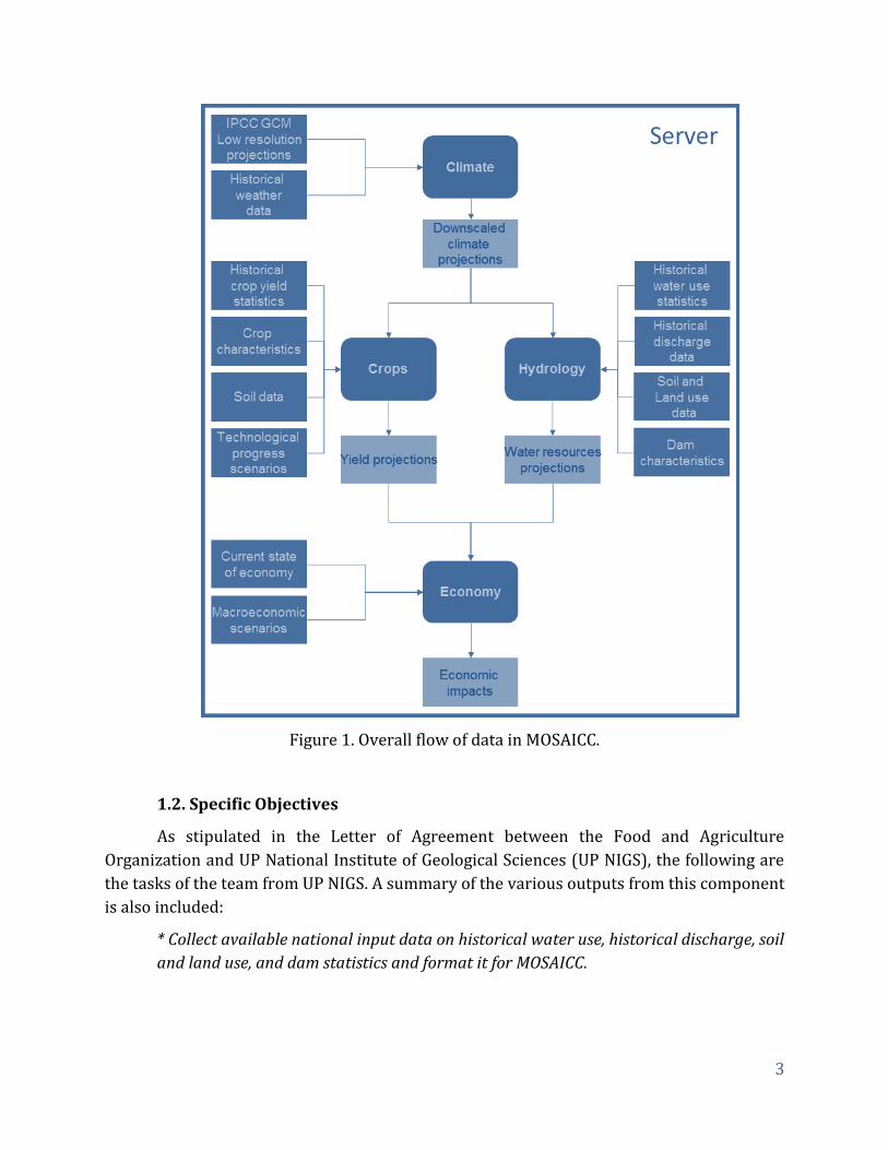
Figure 1. Overall flow of data in MOSAICC.

1.2. Specific Objectives

As stipulated in the Letter of Agreement between the Food and Agriculture

Organization and UP National Institute of Geological Sciences (UP NIGS), the following are

the tasks of the team from UP NIGS. A summary of the various outputs from this component

is also included:

* Collect available national input data on historical water use, historical discharge, soil

and land use, and dam statistics and format it for MOSAICC.

4

- The three volumes of historical stream discharge data (20 years) were

acquired from the Bureau of Research Standards (BRS-DPWH). The entire

data were digitized to produce soft copies of the measurements.

- The watersheds were delineated by the Environment Monitoring

Laboratory in UP NIGS using the ArcHydro software.

- The dam data were acquired from the National Water Resources Board.

* Participate in the trainings for MOSAICC system and its hydrological component.

- Al trainings for STEP 1 Partners were attended:

a. Statistical Climate Downscaling Workshop for PAGASA

b. WABAL Workshop for PhilRice

c. STREAM Workshop for UP NIGS

d. PAM Model Workshop for NEDA

- Training in Wageningen University and Research Centre, Netherlands for

STREAM with Ate Poortinga.

* Participate in the design of an integrated climate change impact study.

- Interpolation of the downscaled climate data was also done since the

climate data output will be used as input for the STREAM model.

* Calibrate the hydrological component of MOSAICC against historical data.

-The stream discharges produced by STREAM for each river were calibrated

using the measured data from the BRS.

* Run the hydrological component of MOSAICC for the study to simulate future projections. Analyze the results of the simulations, making sure the links between upstream/downstream models within MOSAICC, and that the results contribute to the overall study.

-The downscaled climate data has been run for three climate change

scenarios in 8 river basins in the Philippines.

5

1.3. Project Team Composition

The hydrological modeling component was performed by scientists from

Environment Monitoring Laboratory of the University of the Philippines National Institute

of Geological Sciences:

Name Designation

Carlos Primo C. David, Ph.D. Project Leader

Pamela Louise Tolentino Principal Researcher

Justine Perry Domingo Researcher

Maria Teresa Lorenzo Researcher

Peter A. Cayton (Statistician) Statistician

6

Record

Barangay City Province Start End Status

1 Ilocos Norte Laoag Laoag Poblacion Laoag City Ilocos Norte 18-12-12 120-35-18 1984 1994 Fair

2 Cagayan Pared Cagayan Baybayog Alcala Cagayan 17-54-22 121-41-00 1984 1990 Good

3 Nueva Vizcaya Magat Cagayan Baretbet Bagabag Nueva Vizcaya 16-35-02 121-15-06 1985 1992 Good

4 Isabela Ganano Cagayan Ipil Echague Isabela 16-41-56 121-33-06 1987 1992 Good

5 Pampanga Gumain Gumain Sta. Cruz Lubao Pampanga 14-55-00 120-34-08 1985 1996 Fair

6 Nueva Ecija Rio Chico River Pampanga Sto. Rosario Zaragosa Nueva Ecija 15-26-44 120-45-02 1986 1997 Poor

7 Oriental Mindoro Pangalaan Pangalaan Pangalaan Pinamalayan Oriental Mindoro 13-18-9 121-11-45 1990 1999 Good

8 Camarines Sur Yabo Yabo Yabo Sipocot Camarines Sur 13-47-54 122-56-54 1980 1990 Fair

9 Capiz Panay Panay Poblacion Panitan Capiz 11-23-36 123-46-17 1984 1989 Fair

10 Leyte Das-ay Das-ay Sto. Nino II Hinunangan Southern Leyte 10-22-15 125-09-56 1986 2000 Fair

11 Zamboanga del Sur Tukuran Tukuran Tinotongan Tukuran Zamboanga del Sur 7-52-46 123-35-56 1986 2000 Fair

12 Bukidnon Agusan Canyon Agusan Canyon Damilag Manolo Fortich Bukidnon 8-19-22 124-48-26 1990 1999 Fair

13 Sultan Kudarat Allah Cotabato Impao Isulan Sultan Kudarat 6-40-30 124-34-00 1980 1994 NA

14 Agusan del Sur Wawa Agusan Wawa Bayugan Agusan del Sur 8-49-04 125-42-23 1985 1990 Poor

No.Location of the River Year

Irrigated Province River River Basin N E

2. Materials and Methodology

2.1 Study Area

The Philippines is an archipelago in Southeast Asia. It is composed of 7,107 islands

which has a total area of 299,764 square kilometers (sq. km) (Porcil, 2009). There are three

main island groups, Luzon (141,000 sq. km), Visayas (57,000 sq. km) and Mindanao

(102,000 sq. km). The country is divided into 80 provinces, 143 cities and

1491municipalities (NCSB, 2012). The Philippines has 421 principal river basins, 18 of

which are considered as major river basins with at least 1400 sq. km watershed area

(Figure 2) (RBCO, 2013). These river basins are important freshwater resources for

agriculture, commercial and domestic demands. Three of the major river basins are

included in the current study.

Selection of the rivers to be calibrated is based on their geographic location so that

various parts of the country are represented and the availability of the discharge data of

the stream. Fourteen rivers were selected for the study. Table 1 shows information of each

river and Figure 2 shows the location of the rivers. The discharge locations are based on

the established gauging stations of the Bureau of Research Standards (BRS). The basin

maps are generated from STREAM as one of the base maps for the discharge simulations.

Table 1. List of rivers used in STREAM.

7

Figure 2. Upstream maps of the discharge points and their locations in the Philippines.

8

2.2 MOSAICC

The MOSAICC toolbox is based on a generic methodology defined to assess the

impact of climate change on agriculture, including statistical downscaling of climate data,

crop yield projections, water resources estimations and economic modeling. The primary

input of the model is low resolution climate data, which serves as an input for the whole

model structure. This climate data is used to produce the downscaled climate scenarios,

which in turn serves as input data for hydrological modeling and crop growth simulation

modules along with other basic information on elevation, land cover and soil. The outputs

of the hydrological and crop model may then be used as input for the economic model,

which calculates the economic impact. Details of data transformation and analysis for the

hydrological component of MOSAICC are detailed in the succeeding sections.

2.2.1. Climate Downscaling

FAO-MOSAICC utilizes low-resolution projections generated from General

Circulation Models (GCMs) for future climates, similar with most climate change impact

assessment methods. Due to the coarse resolution of GCMs, downscaling is necessary in a

regional or country scale. Projections are statistically downscaled onto particular weather

stations for a specific time period in order to obtain a more precise resolution.

The Santander Meteorology Group of the University of Cantabria, Spain has

developed and incorporated into MOSAICC a statistical downscaling tool for coarse climate

grids generated by GCMs. This tool has been designed to downscale weather variables (i.e.

precipitation, minimum temperature, and maximum temperature) simultaneously for a

weather station network. Three GCMs were used in downscaling climate data, the BCCR-

BCM2.0 (BCM2), the CNRM-CM3 (CNCM3) and the ECHAM5/MPI-OM (MPEH5).

Information on these GCMs are listed in Table 2. Three scenarios were used for the

discharge simulations, (1) 20C3M which is the past climate data (1970-2000), (2) SRES

scenario A1B, which assumes very rapid economic growth, a global population that peaks

in mid-century and rapid introduction of new and more efficient technologies and (3) SRES

scenario A2 which represents the negative extremes, high population growth, slow

economic development and slow technological change. No likelihood has been attached to

any of the SRES scenarios. A1B and A2 are future climate emission scenarios (2011-2050).

9

Atmosphere Ocean Sea Ice Coupling Land

Top Resolution(b) Dynamics, Leads Flux Adjustments Soil, Plants, Routing

Resolution(a) Z Coord., Top BC References References References

References References

1 BCCR-BCM2.0 Bjerknes Centre for Climate top = 10 hPa 0.5°–1.5° x 1.5° L35 rheology, leads no adjustments Layers, canopy, routing

2005 Research, Norway T63 (1.9° x 1.9°) L31 density, free surface Hibler, 1979; Harder, 1996 Furevik et al., 2003 Mahfouf et al., 1995;

Déqué et al., 1994 Bleck et al., 1992 Douville et al., 1995;

Oki and Sud, 1998

2 CNRM-CM3 Météo-France/Centre top = 0.05 hPa 0.5°–2° x 2° L31 rheology, leads no adjustments layers, canopy,routing

2004 National de Recherches T63 (~1.9° x 1.9°) L45 depth, rigid lid Hunke-Dukowicz, 1997; Terray et al., 1998 Mahfouf et al., 1995;

Météorologiques, France Déqué et al., 1994 Madec et al., 1998 Salas-Mélia, 2002 Douville et al., 1995;

Oki and Sud, 1998

3 ECHAM5/MPI-OM Max Planck Institute for top = 10 hPa 1.5° x 1.5° L40 rheology, leads no adjustments bucket, canopy, routing

2005 Meteorology, Germany T63 (~1.9° x 1.9°) L31 depth, free surface Hibler, 1979; Jungclaus et al., 2005 Hagemann, 2002;

Roeckner et al., 2003 Marsland et al., 2003 Semtner, 1976 Hagemann and

Dümenil-Gates, 2001

Sponsor(s), CountryModel ID,

Vintage

Table 2.Information on each GCM used for simulation (Randall et al., 2007).

Notes:

a. Horizontal resolution is expressed either as degrees latitude by longitude or as

a triangular (T) spectral truncation with a rough translation to degrees latitude

and longitude. Vertical resolution (L) is the number of vertical levels.

b. Horizontal resolution is expressed as degrees latitude by longitude, while

vertical resolution (L) is the number of vertical levels.

Spatial consistency can be maintained through different methods incorporated into

the system (e.g. regression, weather typing). A weather generator is included to derive time

series of the weather variables needed. Using both historical weather data and GCMs, the

tool is able to construct climate scenario predictions. The downscaled climate data are

subsequently subjected to different interpolation methods, in order to obtain an

appropriate spatial resolution for hydrological and crop modeling.

2.2.2. Principal Component Analysis

After climate downscaling, the Principal Component Analysis (PCA) is the next step

in order to prepare supporting data. The interpolation tools in MOSAICC have been

designed to process large amounts of data with minimum user input. All interpolation

methods integrated in the system require the following data: 1) digital elevation model

(DEM) of the area of interest, 2) polygon shapefile of the interpolation area, and 3) point

shapefile with the locations of the input weather stations and the input time series.

The main objective is to derive all the maps necessary in subsequent interpolation

procedures. Using the grid data of the input files (DEM and administrative

10

boundaries/river basins), the area of analysis is selected as shown in Figure 3. The

resolution of the interpolation grid can be manipulated through the step value. PCA analysis

will be performed and produce the following grids: interpolation grid, mask of the

interpolation area, grid of the distance to the sea, grids of the first principal components.

These outputs will be the basis for all interpolation methods.

Figure 3.Principal Component Analysis in MOSAICC.

2.2.3. Preliminary Data Interpolation

In order to determine the regression models, Preliminary Data Interpolation

(Prelim), as shown in Figure 4, is performed prior to other interpolation methods. This

function provides additional processes to assist in the determination of the interpolation

parameters. The elements considered for the analysis include geographical and temporal

experiment specifications, stations, predictors and variogram model parameters. Using

these data as input, Prelim executes the following analyses: 1) logarithmic transformation

of the data; 2) stepwise selection of predicting variables for regression model and

diagnosis; and 3) variogram fitting on median values of the regression residuals. Based on

the initial results, the most relevant predictive parameters are selected and the variogram

model values are adjusted for the next interpolation process.

11

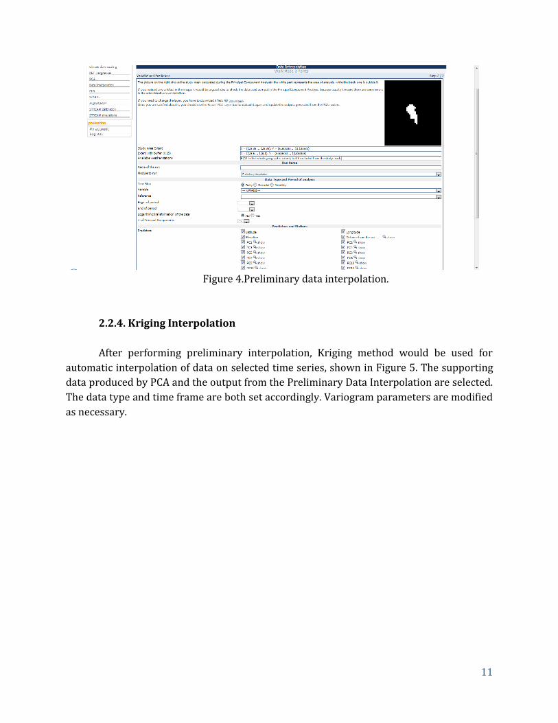
Figure 4.Preliminary data interpolation.

2.2.4. Kriging Interpolation

After performing preliminary interpolation, Kriging method would be used for

automatic interpolation of data on selected time series, shown in Figure 5. The supporting

data produced by PCA and the output from the Preliminary Data Interpolation are selected.

The data type and time frame are both set accordingly. Variogram parameters are modified

as necessary.

12

Figure 5. Data Interpolation through Kriging Method

2.3 STREAM

Calculation of forecasted stream discharge as affected by climate change is

calculated through MOSAICC’s hydrological model called STREAM. The Spatial Tools for

River basins and Environment and Analysis of Management options (STREAM) is a grid-

based spatial water balance model which describes the hydrological cycle of a catchment as

a series of storage compartments and flows (Aerts et al., 1999). The model was developed

to study the processes that impact water availability within a river basin with a specific

focus on the effects of climate change and land use. STREAM has been extensively used for

scenario analysis for a range of different spatial and temporal scales.

STREAM requires spatially explicit input on precipitation, temperature, land-cover

and soil type (Figure 6). From the temperature the evapotranspiration is estimated using

the Thornthwaite equation (Thornthwaite et al., 1957). Based on these parameters, the

water balance is calculated for each grid cell. The former STREAM model uses a flow

routing algorithm to calculate the total runoff, whereas in the new MOSAICC-STREAM it

uses an upstream mask to sum the accumulated runoff. The latter significantly decreases

calculation time and makes it easier to include dams/reservoirs and other compartments

in the calculation.

13

Figure 6. Flowchart of how STREAM model works.

2.3.1. Data requirements

The inputs used for the STREAM model are shown in Table 3.

Table 3: Inputs for the STREAM model

Input Source

Digital Elevation Model (DEM) and basin delineation

Climate Data: precipitation, evaporation or

temperature.

MOSAICC Output (PAGASA/UP

NIGS)

Land use map BSWM

Soil data BSWM

2.3.2. Model Calibration

The hydrological model output also includes a time range from 1979 to 2011

wherein the results can be compared to actual BRS discharge measurements which spans

the years 1980-2000. The datasets’ comparison represents the calibration procedure of the

hydrological model. In the current model calibration scheme, three calibration parameters

are used. These are shown in Table 4.

Precipitation

Soil

Groundwater

Soil type

Land-cover

Temperature

Σ RunoffEvapotranspiration

Snow

14

Table 4.Calibration parameters of STREAM.

Parameter Description Value

C slow flow >1

WATERH water holding capacity

TOGW To groundwater fraction 0 – 1

Model calibration is done in two steps. The first step is done by visually comparing

the actual hydrograph with the predicted hydrograph output, in order to get an estimate

for the different parameters. The actual data is from the stream discharge data from the

Bureau of Research Standards (BRS-DPWH) dataset. The data is presented in a tabulated

form with daily and monthly discharges. The median of the daily measurements were

calculated and compared with the modeled data. Figure 7 shows an example of a page

containing the discharge data. The upper section contains information about the river and

the lower section contains the daily discharge data.

Figure 7.Stream discharge data from the Bureau of Research Standards.

The second step is optimizing the parameters with Model-Independent Parameter

Estimation software (PEST). PEST is a software for model calibration, parameter

estimation and predictive uncertainty analysis. PEST runs the model as many times as

needed adjusting the parameters until the difference between the model output and

measured values approaches a minimum in terms of weighted squares (Doherty, 2004).

15

Hydrological module

Output(discharge

timeseries)

PEST

Control file

PEST

Template file

PEST

Instruction file

PEST

Model input file( groundwater and

Channel velocity)

Figure 8: The PEST optimization scheme.

The PEST optimization routine consists of a control file, template file, module input

file and instruction file as shown in Figure 8. The control file holds all the important

information on parameters, parameter groups, settings and observed values. From a

template file where the parameters are listed a model input file is created. This model input

file can be read by the hydrological module after which the model is run. The output of the

model, a time series of discharge data in this case, is read by PEST following an instruction

file. The predicted data of the model is compared to the observer data, after which the

parameters are adjusted. This process repeats itself until the Gauss-Marquardt-Levenberg

algorithm has found an optimum. The theoretical description of PEST and the Marquardt-

Levenberg algorithm can be found in the manual (Doherty, 2004).

16

2.4 Model Evaluation

To evaluate the model performance in quantitative terms, the Nash and Sutcliffe

Efficiency (NSE) criteria is used. This method is typically developed for hydrological

models. An efficiency of 1 indicates a perfect relation between the predicted and observed

discharge. Negative values indicate a relation which is worse than when the predicted

values would be replaced by the mean observed value. The NSE is defined below:

2meani

T

0 t

2ii

T

0 t

)o(oΣ

)o(pΣ1Efficiency

(1)

where,

omean mean observed value

pi predicted (modeled) values

oi observed values

The median of actual discharge data from BRS are compared with the output

discharge of the model using ERAINT using NSE. The ERAINT were then compared to the

20C3M of each GCM. The NSE between ERAINT and 20C3Ms may be used to determine the

better GCM.

Criss and Winston (2008) discussed the disadvantages on using NSE as a measure of

the model’s efficiency. They reported that NSE tends to overemphasize large flows relative

to other measurements due to squaring of various deviations. According to the them, it can

be a problem since the flows that are more represented in the “goodness-of-fit” calculations

are the least accurately measured. Large negative values may falsely indicate poor

performance of the model, these values may be due to steady observed streamflow. Due to

these problems, another equation was used to determine the efficiency of the model, the

volumetric efficiency (VE). The VE (Equation no. 2) is claimed to be more useful for the

comparison of similarly scaled, rainfall-runoff transfer functions and it treats every cubic

metre of water the same as any other cubic meter, whether it be delivered during slow

recession or during peak flow (Criss and Winston, 2008). VE values are shown in Table 7.

(2)

17

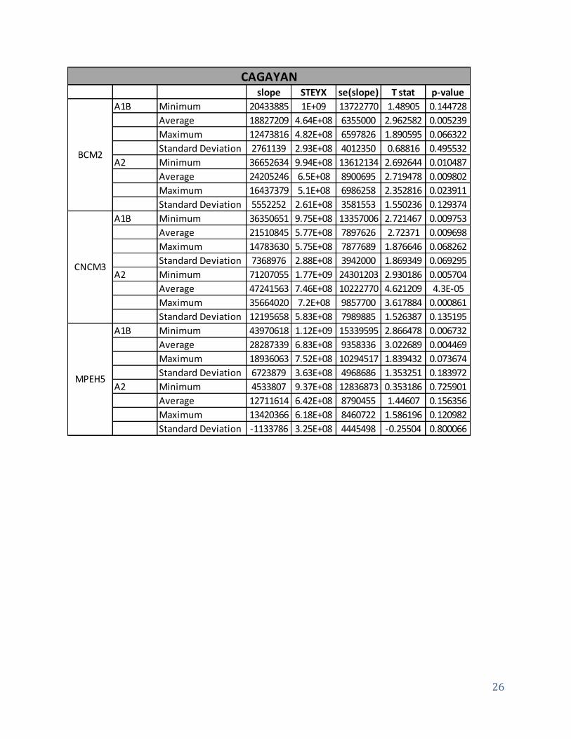
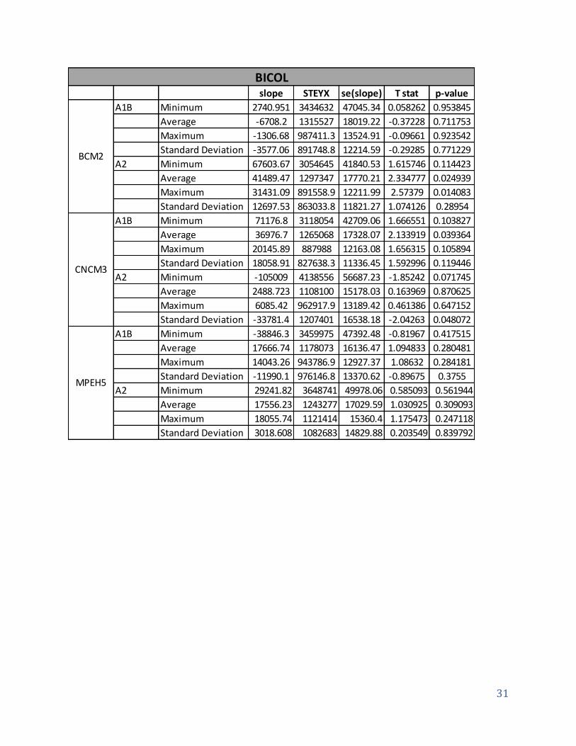
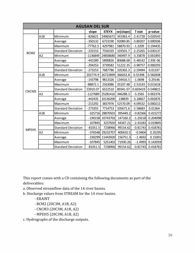
To show the general trend of future discharge projections, the slope and p-value

were computed. Positive value of slope indicates increase in discharge while a negative

value corresponds to decrease in discharge. The p-value determines the significance of this

trend, a value less than or equal to 0.1 indicates that the trend is significant while a value

more than 0.1 indicates that the trend depicted by the slope is not significant.

3. Results and Discussion

3.1 Model Validation

The efficiency of the model was evaluated from the monthly discharges of the

selected river produced by STREAM indicated by ERAINT(converted from cubic meters per

month to cubic meters per second)and the observed monthly median (derived from the

observed daily discharge), using the NSE equation. The ERAINT were also compared with

the 20C3M scenario of each GCM. Table 6 shows the list of the NSE value for each province

for different GCM comparison.

Table 6. NSE measures for each province.

GCM - 20C3M Ilocos Cagayan Nueva Vizcaya Isabela Pampanga Nueva Ecija Bicol

Observed vs ERAINT 0.461293 0.3012 -2.015973035 0.319893148 0.2601508 0.780641408 -0.01963524

ERAINT vs BCM2 0.319351 0.154349 -0.734994203 0.462229126 0.7254823 0.678713054 -3.795062667

ERAINT vs CNCM3 0.227422 -0.40645 -1.858424226 -0.015632554 -0.017777 -0.033821002 -0.453815013

ERAINT vs MPEH5 0.723831 -0.54132 -1.858424226 -0.215816402 0.0306014 0.189180864 -0.453815013

GCM - 20C3M Mindoro Capiz Leyte Zamboanga Bukidnon Sultan Kudarat Agusan del Sur

Observed vs ERAINT -0.00839 -0.03447 -0.006521318 0.142565928 -0.325406 -0.196756787 -0.004566527

ERAINT vs BCM2 -0.98787 -0.36286 0.279729567 0.019121453 -0.266574 -0.20027947 -0.496905863

ERAINT vs CNCM3 -0.47812 -0.27239 0.279729567 -0.031846433 -0.226775 -0.20027947 -0.466111989

ERAINT vs MPEH5 -1.45665 -0.20881 -0.243752355 0.055726249 -0.590043 -0.420314446 0.009222558

18

GCM - 20C3M Ilocos Cagayan Nueva Vizcaya Isabela Pampanga Nueva Ecija Bicol

Observed vs ERAINT 0.77488 0.97130 0.04333 0.82026 -0.00094 0.78934 0.65752

ERAINT vs BCM2 0.91663 0.89395 0.00000 0.93751 0.87406 0.98063 0.00000

ERAINT vs CNCM3 0.95526 0.89801 -0.17202 0.95544 0.85047 0.99452 0.93509

ERAINT vs MPEH5 0.90037 0.93650 -0.17202 0.97683 0.94653 0.94322 0.93509

GCM - 20C3M Mindoro Capiz Leyte Zamboanga Bukidnon Sultan Kudarat Agusan del Sur

Observed vs ERAINT 0.77842 0.97853 0.63853 0.59026 0.80078 0.66147 0.73951

ERAINT vs BCM2 0.85559 0.97255 0.97093 0.77151 0.92974 0.55872 0.90346

ERAINT vs CNCM3 0.82206 0.97423 0.97093 0.89734 0.94206 0.55872 0.87657

ERAINT vs MPEH5 0.27933 0.84459 0.95425 0.84852 0.87601 0.76963 0.99533

Table 7. VE values for each province.

Most of the rivers used in the study for calibration showed negative NSE values but

high VE values. The low to negative values of NSE indicate poor performance of the model

to reproduce the discharge of rivers using historical climate data. Low efficiency values

may be caused by one of the following reasons 1) the model was not able to capture the

actual river setting due to coarse interpolation of climate data, or 2) errors in calibration

due to incorrect measurement of the observed discharge data. The comparison of ERAINT

with the 20C3M scenario of the GCMs also showed poor efficiency.

3.2 Discharge Projection

Ten hydrographs were produced for each river in this study as shown in Figure 8.

The upper graph shows the precipitation (top), temperature (middle) and potential

evapotranspiration (bottom), while the lower graph shows the hydrographs produced for

each GCM. Figure 8a shows the hydrographs of the simulated past discharge using ERAINT

(black) and the hydrograph of the median monthly observed data (blue). Figures 8b, 8c and

8d show the hydrographs of the simulations using ERAINT (green), 20C3M (blue), A1B

(black) and A2 (red). Based from the hydrographs of the simulated and actual discharges,

the model generally underestimated the peak discharges. Nonetheless, the model was able

to capture the periods of peak discharges and simulate the relative changes in river

discharges over specific time periods.

20

Figures 8a-d.Graphs of STREAM output.

3.3 Future Trends Observed

The maximum, average and minimum discharges were computed for the years

2011-2050 for both climate scenarios, A1B and A2.The general trends of the discharges

were examined through slope computation. Figure 9 shows the discharge output of the

model for Nueva Ecija BCM2-A1B. The trendlines of the graphs show that the discharge is

generally increasing, as also implied by the positive slope. The observed increasing trend in

the discharges is significant, as indicated by p-values less than 0.1. The results suggest that

the long-term trend of increasing mean discharge will continue throughout the twenty-first

century. The discharge steadily increases towards year 2050 and there is also an observed

increasing variation in the min/max discharge. This is in accordance with a previous

climate change vulnerability assessment by Jose and Cruz (1999), which suggested that the

expected rise in temperature in the future may not be a significant factor in runoff

variability in particular major reservoirs in the Philippines.

21

(a)

(b)

Figure 9.Plots of the (a) maximum, average, minimum discharges and the (b) standard

deviation of Nueva Ecija BCM2-A1B.

Table 6.Computation of the general trend of projection of river discharge for Nueva Ecija

using BCM2-A1B for years 2011-2050.

NUEVA ECIJA slope se(slope) T stat p-value

BCM2 A1B

3888360.04 1737978.8 2.23728853 0.03121072

2039010.29 630540.333 3.23375077 0.00252929

972062.542 294828.315 3.29704608 0.00212532

1001414.81 532993.989 1.87884822 0.06795207

0

100

200

300

400

500

600

700

800

2010 2015 2020 2025 2030 2035 2040 2045 2050

Mill

ion

s Nueva Ecija BCM2-A1B

Max

Average

Min

0

50

100

150

200

250

2010 2020 2030 2040 2050

Mill

ion

s

Nueva Ecija BCM2-A1B

StDev

22

4. Conclusion and Recommendations

This study used STREAM to simulate projections of river discharge. The model was

able to capture the trend of the peak discharges but the efficiency of the model was found

to be below satisfactory. This suggests that the model can be useful in determining the

discharge patterns for future climate projections. However, further adjustments should be

made, i.e. modification of STREAM with respect to the Philippines’ setting,in order to

increase the robustness of the model and capture the actual discharge better. It could also

be worth trying to calibrate STREAM using the 20C3Mscenarios of the GCMs. A better

projection of the variations of monthly and future river discharges will be useful for the

planning and management of agriculture, irrigation and hydropower production in the

country.

23

5. References

Aerts, J.C.J.H, Kriek, M. and Schepel, M. 1999. STREAM (Spatial Tools for River Basins and

Environment and Analysis of Management Options): ‘Set Up and Requirements’. Phys.

Chem. Earth (B), Vol. 24, No. 26, pp. 591-595.

Dayrit, Hector. 2001. Formulation of a Water Vision. NWRB.In The FAO-ESCAP Pilot Project

on National Water Visions - From Vision to Action - A Synthesis of Experiences in Southeast

Asia. FAO/ESCAP 2001. Reference source:

http://www.fao.org/DOCREP/004/AB776E/ab776e03.htm (Accessed on June 8, 2013)

Doherty, J., 2004. PEST: Model Independent Parameter Estimation. Fifth edition of user

manual. Watermark Numerical Computing, Brisbane, Australia.

Greenpeace. 2007. The State of Water Resource in the

Philippineshttp://www.greenpeace.org/seasia/ph/Global/seasia/report/2007/10/the-

state-of-water-in-the-phil.pdf. (Accessed on June 8, 2013)

Jose, A.M. and Cruz, N.A. 1999. Climate Change Impacts and Responses in the Philippines:

Water Resources. Clim Res. Vol. 12. pp. 77-84.

Harmeling, S. and Eckstein, D. 2012. 2013 Global Climate Risk Index Reference source:

http://germanwatch.org/en/download/7170.pdf(Accessed on June 8, 2013)

Malig, J. 2013, April 6. Quirino temperature soars to 40.1C. ABS-CBNnews.com Reference

source: http://www.abs-cbnnews.com/nation/regions/04/06/13/quirino-temperature-

soars-401c. (Accessed on June 9, 2013)

National Statistical Coordination Board (NCSB). 2012. Philippine Standard Geographic

Code. Reference source:

http://www.nscb.gov.ph/activestats/psgc/publications/NSCB_PSGC_Sep2012.pdf

(Accessed on June 12, 2013)

PAGASA. 2012. Climate in the Philippines. Reference source:

http://kidlat.pagasa.dost.gov.ph/cab/climate.htm (Accessed on June 8, 2013)

Porcil, J. T. 2009. Philippines’ Country Profile. Reference source:

http://www.adrc.asia/countryreport/PHL/2009/PHL2009.pdf(Accessed on June 11,

2013)

http://www.greenpeace.org/seasia/ph/Global/seasia/report/2007/10/the-state-of-water-in-the-phil.pdf

http://www.greenpeace.org/seasia/ph/Global/seasia/report/2007/10/the-state-of-water-in-the-phil.pdf

http://germanwatch.org/en/download/7170.pdf

http://www.abs-cbnnews.com/nation/regions/04/06/13/quirino-temperature-soars-401c

http://www.abs-cbnnews.com/nation/regions/04/06/13/quirino-temperature-soars-401c

http://www.nscb.gov.ph/activestats/psgc/publications/NSCB_PSGC_Sep2012.pdf

http://kidlat.pagasa.dost.gov.ph/cab/climate.htm

http://www.adrc.asia/countryreport/PHL/2009/PHL2009.pdf

24

Randall, D.A., R.A. Wood, S. Bony, R. Colman, T. Fichefet, J. Fyfe, V. Kattsov, A. Pitman, J.

Shukla, J. Srinivasan, R.J. Stouffer, A. Sumi and K.E. Taylor, 2007. Cilmate Models and Their

Evaluation. In: Climate Change 2007: The Physical Science Basis. Contribution of Working

Group I to the Fourth Assessment Report of the Intergovernmental Panel on Climate

Change [Solomon, S., D. Qin, M. Manning, Z. Chen, M. Marquis, K.B. Averyt, M.Tignor and H.L.

Miller (eds.)]. Cambridge University Press, Cambridge, United Kingdom and New York, NY,

USA

River Basin Control Office. 2013. 18 Major River Basins.

http://rbco.denr.gov.ph/index.php/18-major-river-basins/18-major-river-basin (Accessed

on June 12, 2013)

http://rbco.denr.gov.ph/index.php/18-major-river-basins/18-major-river-basin

25

6. Appendix

Future Trend Statistical Analysis

slope STEYX se(slope) T stat p-value

A1B Minimum 6085277 1.43E+08 1961420 3.102485 0.003611

Average 1893265 35216991 482379.3 3.924846 0.000353

Maximum 5747.095 330102.4 4521.527 1.271052 0.211436

Standard Deviation 1891969 47883324 655874.4 2.884651 0.006422

A2 Minimum 1869100 2.45E+08 3355915 0.556957 0.580823

Average 707171.1 55355557 758224.2 0.932668 0.35688

Maximum -15443.8 854252.9 11701 -1.31987 0.194776

Standard Deviation 894831.5 75044937 1027916 0.870529 0.389477

A1B Minimum 3641727 1.22E+08 1665107 2.187083 0.034961

Average 945515.7 32101487 439705.1 2.15034 0.037954

Maximum -7483.06 785134 10754.25 -0.69582 0.490774


A2 Minimum 7198970 2.21E+08 3023691 2.380855 0.022389

Average 1847604 56960372 780205.9 2.368098 0.02307

Maximum 48953.94 4581416 62753.24 0.780102 0.440163

Standard Deviation 2092357 74764661 1024077 2.043163 0.048016

A1B Minimum 7198970 2.21E+08 3023691 2.380855 0.022389

Average 1847604 56960372 780205.9 2.368098 0.02307

Maximum 48953.94 4581416 62753.24 0.780102 0.440163


A2 Minimum 1036469 2.31E+08 3164611 0.327519 0.745073

Average 657234.1 58741503 804602.6 0.816843 0.41911

Maximum -11815.6 945723.6 12953.9 -0.91213 0.367451


ILOCOS

BCM2

CNCM3

MPEH5

26


A1B Minimum 20433885 1E+09 13722770 1.48905 0.144728

Average 18827209 4.64E+08 6355000 2.962582 0.005239

Maximum 12473816 4.82E+08 6597826 1.890595 0.066322

Standard Deviation 2761139 2.93E+08 4012350 0.68816 0.495532

A2 Minimum 36652634 9.94E+08 13612134 2.692644 0.010487

Average 24205246 6.5E+08 8900695 2.719478 0.009802

Maximum 16437379 5.1E+08 6986258 2.352816 0.023911


A1B Minimum 36350651 9.75E+08 13357006 2.721467 0.009753

Average 21510845 5.77E+08 7897626 2.72371 0.009698

Maximum 14783630 5.75E+08 7877689 1.876646 0.068262


A2 Minimum 71207055 1.77E+09 24301203 2.930186 0.005704

Average 47241563 7.46E+08 10222770 4.621209 4.3E-05

Maximum 35664020 7.2E+08 9857700 3.617884 0.000861


A1B Minimum 43970618 1.12E+09 15339595 2.866478 0.006732

Average 28287339 6.83E+08 9358336 3.022689 0.004469

Maximum 18936063 7.52E+08 10294517 1.839432 0.073674


A2 Minimum 4533807 9.37E+08 12836873 0.353186 0.725901

Average 12711614 6.42E+08 8790455 1.44607 0.156356

Maximum 13420366 6.18E+08 8460722 1.586196 0.120982

Standard Deviation -1133786 3.25E+08 4445498 -0.25504 0.800066

BCM2

CNCM3

MPEH5

CAGAYAN

27


A1B Minimum 665342.2 19753589 270571.7 2.459023 0.018598

Average 516845.4 10077353 138033 3.744361 0.000598

Maximum 298766.2 10899012 149287.5 2.00128 0.052541

Standard Deviation 113787.6 7071335 96858.52 1.174781 0.247392

A2 Minimum 1015113 19479147 266812.6 3.804593 0.000502

Average 580392 12880606 176430.1 3.289643 0.002169

Maximum 330073 10521347 144114.5 2.290352 0.027641


A1B Minimum 860558.6 19065277 261143.7 3.295346 0.002135

Average 513841.7 12089938 165600.1 3.102908 0.003607

Maximum 264119.6 13508341 185028.4 1.427454 0.161616


A2 Minimum 1629020 39201098 536951 3.033833 0.004339

Average 1027697 15754365 215793 4.762423 2.78E-05

Maximum 696315.3 13772782 188650.5 3.691033 0.000698


A1B Minimum 1121889 23758372 325426.6 3.447442 0.001398

Average 685771.7 14751287 202053.5 3.394011 0.001623

Maximum 379113 18296893 250618.9 1.512708 0.138627


A2 Minimum 251100.6 20808891 285026.6 0.880973 0.383871

Average 343547.9 13651739 186992.6 1.837227 0.074006

Maximum 311221.6 14256393 195274.7 1.593763 0.119274

Standard Deviation -35436.2 8439244 115595.2 -0.30655 0.760856

ISABELA

BCM2

CNCM3

MPEH5

28


A1B Minimum 9463001 1.82E+08 2496156 3.79103 0.000522

Average 4270836 67919633 930318.7 4.590724 4.73E-05

Maximum 1265304 37108431 508287 2.48935 0.017292


A2 Minimum 7814281 2.11E+08 2895553 2.698718 0.010328

Average 3888126 88541412 1212782 3.205955 0.002729

Maximum 1129152 43982702 602446.2 1.874278 0.068595


A1B Minimum 6702777 1.37E+08 1873279 3.578099 0.000965

Average 3389474 65816808 901515.5 3.759752 0.000572

Maximum 972154.4 51998813 712245.7 1.364914 0.180308


A2 Minimum 15781598 2.59E+08 3549270 4.446435 7.35E-05

Average 7372822 97805452 1339675 5.503441 2.73E-06

Maximum 2860927 62159139 851415.2 3.360202 0.001784


A1B Minimum 10575897 2.27E+08 3111774 3.398671 0.001602

Average 5106827 83682394 1146227 4.455338 7.16E-05

Maximum 1835302 77218581 1057690 1.735199 0.09081


A2 Minimum 2438020 2.22E+08 3041138 0.80168 0.427723

Average 2336132 95911299 1313730 1.778243 0.083366

Maximum 1189919 60220550 824861.7 1.442568 0.157335


NUEVA VIZCAYA

BCM2

CNCM3

MPEH5

29


A1B Minimum 1194600 83546925 1144371 1.043892 0.303131

Average 684699.8 20167641 276243.1 2.478613 0.017745

Maximum 102453 3352797 45924.42 2.230904 0.031667


A2 Minimum 1716334 64050367 877320 1.956337 0.057805

Average 363863.6 13635598 186771.5 1.948175 0.058808

Maximum 48392.88 2569704 35198.12 1.374871 0.177225


A1B Minimum 2660604 67755247 928067 2.866823 0.006726

Average 880247.8 14452715 197963.8 4.446508 7.35E-05

Maximum 128710.4 2232161 30574.68 4.209705 0.000151


A2 Minimum 2684459 1.01E+08 1385348 1.937751 0.060111

Average 1049750 27065112 370720.2 2.83165 0.007365

Maximum 168849.7 4216088 57749.21 2.923845 0.005799


A1B Minimum 2144327 70860220 970596.9 2.209287 0.033256

Average 609148.7 21162496 289870 2.101455 0.042287

Maximum 97849.61 3319217 45464.46 2.152222 0.037796


A2 Minimum 1455339 88648878 1214254 1.198545 0.238126

Average 638044.9 25058910 343240.5 1.858886 0.070801

Maximum 89502.51 3380540 46304.42 1.932915 0.060724


PAMPANGA

BCM2

CNCM3

MPEH5

30


A1B Minimum 3888360 1.27E+08 1737979 2.237289 0.031211

Average 2039010 46033763 630540.3 3.233751 0.002529

Maximum 972062.5 21524486 294828.3 3.297046 0.002125


A2 Minimum 3902711 88274602 1209128 3.227708 0.002571

Average 1651231 27129323 371599.7 4.443574 7.42E-05

Maximum 728470.9 11655735 159652.6 4.562849 5.15E-05


A1B Minimum 5751722 93386042 1279141 4.496551 6.31E-05

Average 2567714 28250307 386954.2 6.635705 7.68E-08

Maximum 1235314 14088199 192970.9 6.401554 1.6E-07


A2 Minimum 6709741 1.7E+08 2327289 2.883072 0.006449

Average 3633090 52341396 716938.2 5.067509 1.08E-05

Maximum 1907492 27053147 370556.3 5.147645 8.36E-06


A1B Minimum 4869032 1.13E+08 1543941 3.153638 0.003146

Average 2146756 41509460 568569.4 3.775716 0.000546

Maximum 1224746 21373835 292764.8 4.18338 0.000163


A2 Minimum 2494552 1.57E+08 2148833 1.160887 0.252929

Average 2014662 55235789 756583.7 2.662841 0.011299

Maximum 1166309 21950200 300659.5 3.87917 0.000403


NUEVA ECIJA

BCM2

CNCM3

MPEH5

31


A1B Minimum 2740.951 3434632 47045.34 0.058262 0.953845

Average -6708.2 1315527 18019.22 -0.37228 0.711753

Maximum -1306.68 987411.3 13524.91 -0.09661 0.923542

Standard Deviation -3577.06 891748.8 12214.59 -0.29285 0.771229

A2 Minimum 67603.67 3054645 41840.53 1.615746 0.114423

Average 41489.47 1297347 17770.21 2.334777 0.024939

Maximum 31431.09 891558.9 12211.99 2.57379 0.014083

Standard Deviation 12697.53 863033.8 11821.27 1.074126 0.28954

A1B Minimum 71176.8 3118054 42709.06 1.666551 0.103827

Average 36976.7 1265068 17328.07 2.133919 0.039364

Maximum 20145.89 887988 12163.08 1.656315 0.105894


A2 Minimum -105009 4138556 56687.23 -1.85242 0.071745

Average 2488.723 1108100 15178.03 0.163969 0.870625

Maximum 6085.42 962917.9 13189.42 0.461386 0.647152


A1B Minimum -38846.3 3459975 47392.48 -0.81967 0.417515

Average 17666.74 1178073 16136.47 1.094833 0.280481

Maximum 14043.26 943786.9 12927.37 1.08632 0.284181


A2 Minimum 29241.82 3648741 49978.06 0.585093 0.561944

Average 17556.23 1243277 17029.59 1.030925 0.309093

Maximum 18055.74 1121414 15360.4 1.175473 0.247118


BICOL

BCM2

CNCM3

MPEH5

32


A1B Minimum 2123536 72870417 998131.2 2.127512 0.039926

Average 1615795 24497534 335551.2 4.815347 2.36E-05

Maximum 708359.1 21796537 298554.7 2.372628 0.022826


A2 Minimum 2233445 1.52E+08 2081924 1.072779 0.290136

Average 1738016 27791448 380669.1 4.565688 5.1E-05

Maximum 904479.9 34642209 474506.3 1.90615 0.064215


A1B Minimum 1598441 1.33E+08 1816238 0.880084 0.384346

Average 1682407 36162183 495325.9 3.396566 0.001612

Maximum 990958.6 30304753 415094.7 2.387308 0.022052


A2 Minimum 2336000 1.52E+08 2085364 1.120188 0.269664

Average 1798991 28602640 391780.2 4.591838 4.71E-05

Maximum 921636.6 35314654 483717 1.905322 0.064326


A1B Minimum 2168816 83479652 1143450 1.896731 0.065484

Average 1773271 28927547 396230.6 4.475352 6.73E-05

Maximum 715905.6 22254294 304824.7 2.348581 0.024149


A2 Minimum 3167274 1.06E+08 1452267 2.180917 0.035448

Average 2449222 24759131 339134.4 7.221983 1.23E-08

Maximum 750878.5 19001112 260264.8 2.885056 0.006416


MPEH5

CNCM3

BCM2

MINDORO

33


A1B Minimum 1762530 66938524 916880.1 1.922312 0.062087

Average 762744.2 22978496 314744.4 2.423377 0.020248

Maximum 562027.6 15997976 219129.8 2.564816 0.014396


A2 Minimum -1133152 1.09E+08 1494361 -0.75829 0.452958

Average -454020 33050623 452705.8 -1.0029 0.322251

Maximum -292.286 26265016 359761 -0.00081 0.999356

Standard Deviation -526167 37397527 512246.8 -1.02717 0.310833

A1B Minimum -1636606 1.04E+08 1430940 -1.14373 0.259891

Average -571286 27670976 379018.9 -1.50727 0.140009

Maximum -44547.7 24381525 333962.2 -0.13339 0.894588


A2 Minimum -1044735 1.07E+08 1471792 -0.70984 0.482138

Average -365562 33445682 458117.1 -0.79797 0.429848

Maximum 41963.43 26606265 364435.2 0.115146 0.908935


A1B Minimum 744255.9 83073469 1137886 0.654069 0.517006

Average 1630289 29831430 408611.4 3.989828 0.000291

Maximum 1203352 20836616 285406.3 4.216276 0.000148


A2 Minimum 1088569 97898920 1340955 0.811786 0.42197

Average 1211799 22678809 310639.5 3.900981 0.000378

Maximum 811287.9 18136749 248425.3 3.265722 0.002317


MPEH5

CNCM3

BCM2

CAPIZ

34


A1B Minimum -41060.5 3552118 48654.59 -0.84392 0.403997

Average -36704.3 1134100 15534.16 -2.36281 0.023358

Maximum -15315.1 1053401 14428.79 -1.06143 0.295196


A2 Minimum -148084 3383176 46340.53 -3.19557 0.002807

Average -62008.1 1478861 20256.47 -3.06115 0.004034

Maximum -38824.4 1117110 15301.45 -2.5373 0.015396


A1B Minimum 18318.59 3313785 45390.06 0.403582 0.688783

Average -18272.7 1319264 18070.41 -1.0112 0.318319

Maximum -16645.5 1002132 13726.55 -1.21265 0.232749


A2 Minimum -150429 3438186 47094.02 -3.19422 0.002818

Average -61489.1 1492053 20437.17 -3.00869 0.004638

; -36517.7 1162940 15929.2 -2.2925 0.027504


A1B Minimum -58691.8 3162176 43313.42 -1.35505 0.183403

Average -12468.7 1578939 21627.28 -0.57653 0.567659

Maximum -9617.7 1027350 14071.97 -0.68347 0.49846


A2 Minimum -98300.7 3164154 43340.5 -2.2681 0.029091

Average -30506.5 1408049 19286.53 -1.58175 0.121995

Maximum -7043.81 894458.8 12251.71 -0.57492 0.568731


CNCM3

MPEH5

LEYTE

BCM2

35


A1B Minimum -66420.5 5721179 78364.97 -0.84758 0.401979

Average -8890.75 958871.4 13133.99 -0.67693 0.502553

Maximum -3562.64 395054 5411.191 -0.65838 0.514261


A2 Minimum -7158.52 10634853 145669.2 -0.04914 0.961063

Average -24135.8 1280298 17536.68 -1.37631 0.176784

Maximum -10343.1 816468.3 11183.45 -0.92486 0.360874


A1B Minimum -174838 9136771 125149.5 -1.39703 0.17051

Average -65470.1 1209014 16560.29 -3.95344 0.000324

Maximum -13216.7 671562.3 9198.621 -1.43682 0.158953


A2 Minimum -174838 9136771 125149.5 -1.39703 0.17051

Average -65470.1 1209014 16560.29 -3.95344 0.000324

Maximum -13216.7 671562.3 9198.621 -1.43682 0.158953


A1B Minimum -174838 9136771 125149.5 -1.39703 0.17051

Average -65470.1 1209014 16560.29 -3.95344 0.000324

Maximum -13216.7 671562.3 9198.621 -1.43682 0.158953


A2 Minimum -174838 9136771 125149.5 -1.39703 0.17051

Average -65470.1 1209014 16560.29 -3.95344 0.000324

Maximum -13216.7 671562.3 9198.621 -1.43682 0.158953


MPEH5

CNCM3

BCM2

ZAMBOANGA

36


A1B Minimum 1807.055 3516240 48163.15 0.037519 0.970267

Average -4872.04 923102.8 12644.06 -0.38532 0.702147

Maximum 2909.54 487676.4 6679.872 0.435568 0.665614


A2 Minimum -175619 5270672 72194.21 -2.4326 0.019809

Average -84615.5 1451225 19877.93 -4.25676 0.000131

Maximum -29410 537532.4 7362.766 -3.99443 0.000287


A1B Minimum -110900 4215165 57736.57 -1.92079 0.062284

Average -49453 1099648 15062.26 -3.28324 0.002208

Maximum -12025.5 494099.3 6767.849 -1.77685 0.083598


A2 Minimum -174777 5356844 73374.55 -2.38198 0.02233

Average -86935.2 1513650 20732.98 -4.19309 0.000159

Maximum -30750.1 545779.5 7475.731 -4.11333 0.000201


A1B Minimum -57462.9 3354093 45942.18 -1.25077 0.218667

Average 148.3198 1382635 18938.43 0.007832 0.993792

Maximum 12589.55 576617.5 7898.129 1.593991 0.119223


A2 Minimum -17469.2 4182719 57292.14 -0.30492 0.762095

Average 18502.13 1143533 15663.37 1.181235 0.24485

Maximum 8099.436 584828.7 8010.601 1.01109 0.318369


MPEH5

CNCM3

BCM2

BUKIDNON

37


A1B Minimum -493665 21431231 293551 -1.6817 0.100829

Average -224450 3523382 48260.98 -4.65075 3.93E-05

Maximum -21925.7 3475098 47599.62 -0.46063 0.647692


A2 Minimum -416255 37803806 517811.8 -0.80387 0.42647

Average -191131 6499697 89028.59 -2.14685 0.03825

Maximum -65003 5456994 74746.33 -0.86965 0.389953

Standard Deviation -131487 13661479 187126 -0.70266 0.486548

A1B Minimum -748938 36033579 493564.4 -1.51741 0.13744

Average -275368 6958969 95319.39 -2.88889 0.006352

Maximum -62799.5 6408148 87774.62 -0.71546 0.478696


A2 Minimum -443912 39085191 535363.3 -0.82918 0.412181

Average -204084 6870467 94107.16 -2.16864 0.036436

Maximum -74864.1 5619929 76978.11 -0.97254 0.336934

Standard Deviation -141509 14178735 194211 -0.72864 0.47069

A1B Minimum 611595 40788894 558699.6 1.094676 0.280549

Average 260258.7 6608706 90521.73 2.875096 0.006584

Maximum 103167 5899767 80811.15 1.276643 0.209475


A2 Minimum 1109197 38828448 531846.7 2.085558 0.043786

Average 517056.4 4500364 61643.04 8.387912 3.56E-10

Maximum 159559.4 4528285 62025.48 2.572481 0.014129


MPEH5

CNCM3

BCM2

SULTAN KUDARAT

38

This report comes with a CD containing the following documents as part of the

deliverables:

a. Observed streamflow data of the 14 river basins.

b. Discharge values from STREAM for the 14 river basins.

- ERAINT

- BCM2 (20C3M, A1B, A2)

- CNCM3 (20C3M, A1B, A2)

- MPEH5 (20C3M, A1B, A2)

c. Hydrographs of the discharge outputs.


A1B Minimum -826621 24965672 341963.4 -2.41728 0.020543

Average -350132 6723190 92089.85 -3.80207 0.000506

Maximum -77762.5 4297981 58870.93 -1.3209 0.194435


A2 Minimum -1136849 24858680 340497.9 -3.33878 0.001893

Average -442289 5890826 80688.68 -5.48142 2.93E-06

Maximum -204253 3739582 51222.35 -3.98757 0.000293


A1B Minimum 202774.9 26722899 366032.8 0.55398 0.582838

Average -143798 9813326 134416.5 -1.0698 0.29146

Maximum -88872.1 2563086 35107.48 -2.53143 0.015618


A2 Minimum -1127689 25281416 346288.3 -3.2565 0.002376

Average -442435 10136200 138839 -3.18667 0.002876

Maximum -215292 3837976 52570.09 -4.09532 0.000213


A1B Minimum -325716 28870501 395449.2 -0.82366 0.415272

Average -190158 10743702 147160.2 -1.29218 0.204098

Maximum -107845 3237650 44347.21 -2.43183 0.019845


A2 Minimum -376548 29232707 400410.5 -0.9404 0.35295

Average -230299 11443920 156751.3 -1.4692 0.15001

Maximum -107845 5251402 71930.26 -1.4993 0.142059


MPEH5

CNCM3

BCM2

AGUSAN DEL SUR

analysis of climate change impacts on stream discharges ... · analysis of climate change impacts...

Documents