Use of stream response functions to determine impacts of replacingsurface-water use with groundwater withdrawals

Erik B. Pruneda & Michael E. Barber &

Diana M. Allen & Joan Q. Wu

Abstract A regional-scale numerical groundwater modelis used to study the impacts of replacing surface-water usewith groundwater wells to improve low-flow streamconditions for endangered species within the Bertrandand Fishtrap watersheds, southern British Columbia,Canada and Washington, USA. Stream response functionsranging from 0 to 1.0 were calculated for individual wellsplaced within a steady-state groundwater flow model atvarying distances from the streams to determine theimpact that these replacement wells, operating undersustained pumping rates, would have on summer instreamflows. Lower response ratios indicate groundwater pump-ing will have less of an impact on streamflow than takingan equivalent amount of water directly from a surface-water source. Results show that replacing surface-wateruse with groundwater withdrawals may be a viablealternative for increasing summer streamflows. Assumingcombined response factors should be ≤0.5 for irrigators toundergo the expense of installing new wells, ~57% of theland area within 0.8km of Bertrand Creek would besuitable for replacement wells. Similarly, 70% of the landarea within 0.8km of Fishtrap Creek was found to be

appropriate. A visual analysis tool was developed usingSTELLA to allow stakeholders to quickly evaluate theimpact associated with moving their water right.

Keywords Groundwater/surface-water relations . Streamresponse functions . Water-resources conservation .Numerical modeling . Canada . USA

Introduction

Consumption of water for municipal and irrigation usescan have adverse impacts on minimum instream flowsnecessary for ecosystem health. In the Pacific Northwest,USA and southern British Columbia, Canada, thisproblem is most acute during summer and early fallmonths when dry weather and increased demands combineto create severe water shortages in many streams (e.g.,Adelsman 2003). Recent instream flow studies on twowatersheds in northwest Washington (Bertrand andFishtrap Creeks) found that summer flows are too lowto support desired salmon uses (WAC 173-501-0301985; Kemblowski et al. 2002). The problem is notlimited to surface-water use, as many groundwater with-drawals from wells completed within the shallow alluvialaquifer nearby the streams cause significant decreases instreamflow through surface water and groundwater inter-action (Winter et al. 1998; Hantush 2005).

An innovative way to manage water demand isneeded to help alleviate the problem in this and similarwatersheds. One proposed alternative involves replacingsurface-water use with groundwater withdrawals. Whileremoving surface-water use will keep the previouslyused water in the stream, the overall net effect onstreamflow will depend on the location of replacementwells and aquifer and streambed properties. Essentially,groundwater pumping wells should be far enough awayfrom the streams so as not to have a negative effect onstreamflow, either within some specified time period (i.e.,a transient response) or indefinitely (i.e., steady-stateresponse).

Understanding the interaction between surface waterand groundwater is the key to accurately predicting thelikelihood of success for this alternative. Numerousapproaches have been used to investigate surface water

Received: 20 July 2009 /Accepted: 10 February 2010Published online: 10 March 2010

* Springer-Verlag 2010

E. B. Pruneda :M. E. BarberCivil and Environmental Engineering,Washington State University,PO Box 643002, Pullman, WA 99164-3002, USA

M. E. Barbere-mail: meb@wsu.edu

J. Q. WuDepartment of Biological Systems Engineering,Washington State University,PO Box 646120, Pullman, WA 99164-3002, USAe-mail: jwu@wsu.edu

D. M. Allen ())Department of Earth Sciences,Simon Fraser University,8888 University Drive, Burnaby, BC V5A 1S6, Canadae-mail: dallen@sfu.caTel.: +1-778-7823967

Hydrogeology Journal (2010) 18: 1077–1092 DOI 10.1007/s10040-010-0591-3

and groundwater interaction ranging from analyticalapproximations (Cooper and Rorabaugh 1963; Jenkins1968a; Moench and Barlow 2000) to combined analyticaland numerical solutions (Leake et al. 2008a) to entirelynumerical solutions (Pinder and Sauer 1971; Saquillace1996; Chen and Chen 2003; Leake and Reeves 2008; Leakeet al. 2008b) with the strengths and weaknesses of bothapproaches being discussed in the literature (Sharp1977; Perkins and Koussis 1996). The methodologyused in this study combines a steady-state numericalMODFLOW model (Harbaugh et al. 2000) implementedwithin Visual MODFLOW version 4.1 (Waterloo Hydro-geologic Inc. 2006) with the linear response theory firstproposed by Morel-Seytoux (1975) to develop streamresponse functions.

The effects of a groundwater withdrawal propagateradially until they reach a boundary condition such as ano-flow or recharge boundary. As the effects reach arecharge boundary such as a hydraulically connectedstream, the result is either a decrease in stream gain oran increase in stream loss. As noted by Jenkins (1968a), ininfinite time (at steady state), the full aquifer withdrawalwill be drawn from a hydraulically connected rechargeboundary. In a large developed groundwater system,evaluation of the impacts of multiple groundwater stresseson stream reaches or aquifer water levels over longperiods of time can be a complicated process. Responsefunctions can be used to describe the spatial and temporalpropagation of such impacts.

Response functions can be generated using eitheranalytical techniques or a numerical model. Analyticaltechniques are typically subject to restrictive or simplifyingassumptions (Cosgrove and Johnson 2004). For example,Jenkins (1968a) assumes a straight, fully penetrating streamin a homogeneous aquifer to determine response functions ofstream depletion by wells. Generating response functionsusing a numerical groundwater model enables the represen-tation of complex system heterogeneities and anisotropies.For example, Barlow et al. (2003) and Cosgrove andJohnson (2004) demonstrated the use of stream responsefunctions within a groundwater flowmodel to study the localgroundwater and surface-water interactions. The goal inboth of these studies was to create stream response functionsthat would allow the impacts of groundwater pumping onsurface-water flows to be quantified.

Using a response-matrix technique, Barlow et al. (2003)coupled a numerical groundwater model and optimizationtechniques to maximize total groundwater withdrawal fromthe Hunt-Annaquatucket-Pettaquamscutt stream-aquifer ofcentral Rhode Island, during the summer months of July,August and September, while maintaining desired streamflows. Response functions were generated for 14 publicwater supply wells and two hypothetical wells. Barlow etal. (2003) assumed the rate of stream flow depletion at aconstraint site to be a linear function of the pumping rate ofeach groundwater well. By assuming linearity, the conceptof superposition allowed for individual stream flowdepletions caused by each well to be summed together ata constraint site to derive a total stream flow depletion.

Cosgrove and Johnson (2004) modified an existingsingle layer, unconfined, transient MODFLOW (Harbaughet al. 2000) groundwater model for the Snake River PlainAquifer, Idaho, for use with the MODRSP code (Maddockand Lacher 1991) to generate response functions. Theunconfined groundwater model was converted to aconfined system, to conform to the MODRSP requirementof modeling a linear system. Transient response functionsfor 51 river cells were generated for each of the numericalmodel cells using 150 4-month stress periods representing50 years. The response functions are a result of a unitstress applied only during the first stress period and, as aresult, they represent the propagation of the effects of thatunit stress over time. Making use of the transient responsefunctions, a spreadsheet was developed that allows theuser to enter water-use scenarios and determine the impactto surface-water resources.

Leake and Reeves (2008) describe a procedure andconsiderations for using groundwater flow models toconstruct maps that illustrate the distribution and timingof capture of natural discharge due to pumping. Three typesof maps described in their paper include: (1) transientcapture from all head-dependent flow boundaries, (2)transient capture from a particular head-dependent flowboundary, and (3) ultimate steady-state capture from aparticular head-dependent flow boundary. Leake et al.(2008b) show spatial distributions of total change in inflowand outflow from withdrawal or injection for select times ofinterest for the Sierra Vista Subwatershed and the Sonora,Mexico, portion of the Upper San Pedro Basin in the USA.Maps of transient capture of discharge to all MODFLOWhead-dependent flow boundaries were constructed. Themapped areal distributions show the effect of a single wellin terms of the ratio of the change in boundary flow rate torate of withdrawal or injection by the well. To the extentthat the system responds linearly to groundwater with-drawal or injection, fractional responses in the mappeddistributions can be used to quantify response for anywithdrawal or injection rate.

The overall objective of this research was to determinethe impacts of exchanging surface-water sources forgroundwater wells on streamflows in Bertrand and FishtrapCreeks. A regional-scale steady-state groundwater flowmodel, developed previously for the aquifer (Scibek andAllen 2005) was used. Because of its regional scale, thegroundwater flow model contained insufficient localizedinformation to accurately examine groundwater and sur-face-water interactions for specific stream reaches. There-fore, the model was refined locally using measured seepagedata from Bertrand and Fishtrap Creeks, local groundwaterand surface-water elevations, streambed hydraulic conduc-tivities, and additional groundwater pumping well locationsand rates of extraction. Stream response functions werethen determined by sequentially adding groundwaterextraction wells to the model at increasing distances fromthe stream to determine the net effect on the steady-statestream water budget. A steady-state model was used tofacilitate the development of a decision support systemimplemented in STELLA (isee Systems 2007) for evaluating

1078

Hydrogeology Journal (2010) 18: 1077–1092 DOI 10.1007/s10040-010-0591-3

the impacts. Specifically, the simulated stream responsefunctions were incorporated into a STELLA model thatallows the user to simulate the effects on the instream flowsof Bertrand and Fishtrap Creeks through exchanging asurface-water source for a single replacement groundwaterwell of the same withdrawal rate, without the need to run thegroundwater flow model.

Background

The study site is situated within the Abbotsford-Sumasaquifer, which extends from southern British Columbia,Canada, southward into northern Washington, USA(Fig. 1). The aquifer is the largest aquifer in the region,covering an area of approximately 161 km2, and isroughly bisected by the Canada-USA border. The aquiferis also highly productive, and provides water supply fornearly 10,000 people in the USA (towns of Sumas,Lynden, Ferndale, Everson and scattered agriculturalestablishments) and 100,000 in Canada, mostly in the cityof Abbotsford, but also in the township of Langley(Mitchell et al. 2003). In the 1990s, the region was

described as having population and industrial growth thatwas among the fastest in North America (Boyle et al.1997). These development pressures are continuing andplace strain on the water resources in the area, throughoutboth the Canada and the USA portions of the aquifer.

The Abbotsford-Sumas aquifer is located on a broadoutwash plain, which is elevated above the adjacent riverfloodplains (Fig. 1); topographic relief is roughly 150 m.The uplands are centered on the city of Abbotsford, BCand extend westward through Langley, BC and south toLynden, WA. The largest valley is Sumas Valley, whichruns north-east to south-west from the city of Sumas to thecity of Chilliwack (Fig. 1), and contains the lowerdrainage of the Sumas River. The Sumas River flows tothe northeast and picks up a significant baseflow compo-nent from aquifer discharge on its eastern side. To thesouth is the Nooksack River, which flows west and thensouth. Most of the surface and groundwater flow fromthe Abbotsford-Sumas aquifer ends up in the NooksackRiver. To the north is the Fraser River, which does notreceive any significant discharge from this aquifer as itlies to the north of the topographic high and groundwaterdivide.

Fraser River

ABBOTSFORD

Sumas Mt.(BC)

CHILLIWACK

British Columbia, Canada

Washington, USA

0 1 2 3

0 1 2 3 4 5

Miles

Kilometers

Vedder Mt

SumasRiver

490

-122.50

Bertr

and

Cr.

Fish

trap

Cr.

Pep

inB

r.

Canada

USA

Mexico

StudyArea

Model domain

Study areaoutline

Aquifer outline

Abbotsford-Sumas Aquifer

Sumas Mt. (WA)

Nooksack R.

FERNDALE

LANGLEY

LYNDEN

EVERSON

SUMAS

Fig. 1 Location of study area in southwestern British Columbia, Canada, and northwestern Washington State, USA. The internationalborder is shown. The Abbotsford-Sumas aquifer is shaded, and the outline of the groundwater model domain is shown by a dashed line.The model domain encompasses the Fishtrap and Bertrand Creek watersheds, which drain to the Nooksak River

1079

Hydrogeology Journal (2010) 18: 1077–1092 DOI 10.1007/s10040-010-0591-3

The climate in this coastal region is humid and temperate,with warm, dry summers and mild, wet winters. Meanannual precipitation ranges from 1,000 to 2,100 mm (N–Sgradient) and falls mostly as rain. Roughly 18% ofprecipitation falls during the months of June throughSeptember, and 82% during the months of October throughMay (McKenzie 2007). Recharge to the aquifer (900–1,100 mm) is primarily from direct precipitation (Scibekand Allen 2006).

The aquifer is mostly unconfined (it becomes confinedunder Sumas Valley) and is comprised of Quaternary agecoarse-grained sediments of glaciofluvial drift origin,referred to as the Sumas Drift (11,000–10,000 BP)(Armstrong et al. 1965). The Sumas Drift consists ofdiamictons (lodgement and flow tills), thick and well-sorted glaciofluvial outwash (uncompacted) sands andgravels (advance and recessional), glaciolacustrine sedi-ments, and ice-contact sediments deposited during theSumas Stade of the Fraser Glaciation (Armstrong et al.1965). It also contains lenses of till. The thickness ofSumas Drift can be up to 65 m, and it is thickest in thenortheast where glacial terminal moraine deposits arefound. The aquifer is underlain by an extensive glacio-marine deposit, the Fort Langley Formation/Everson,which outcrops in the uplands to the northwest (LangleyUplands) and southeast (Sumas Valley). The Tertiary agebedrock surface underlying the unconsolidated deposits isapproximately 210 m below the ground surface (Scibekand Allen 2005). Soils over the aquifer are generally thin(approximately <0.7 m thick) with permeability thatexceeds precipitation rates (Mitchell et al. 2003).

Recharge to the aquifer is predominantly by directprecipitation (Scibek and Allen 2005). The average annualvariation in water levels in the aquifer is 2 m, with amaximum variation estimated by Scibek and Allen (2005)as 3 m. There is approximately a 3-month lag periodbetween minimum precipitation and minimum water tablelevels. Groundwater flows regionally from north to south,although there are some local variations (Scibek and Allen2005), particularly in the vicinity of the streams that drainthe aquifer.

The research focuses on two main streams that drainthe aquifer, namely Fishtrap Creek and Bertrand Creek.Situated between these two streams is Pepin Brook, whichis a tributary to Fishtrap Creek south of the internationalborder. Combined, the watersheds cover approximately100 km2. Approximately 46% of the Bertrand watershed(50.2 km2) and 39% of the Fishtrap watershed (37.3 km2)are within the USA, with the remaining areas extendinginto Canada. Bertrand Creek is a naturally formed,meandering stream, whereas Fishtrap Creek has beenchannelized in many places to accommodate agricultureand to reduce flooding. The predominant land use withinboth countries for both watersheds is agricultural.

Fishtrap and Bertrand Creeks originate at relatively lowelevation (slightly above mean sea level) and the flowregime is driven by precipitation and interaction with thegroundwater (Berg and Allen 2007). The flow regimemimics the timing of the precipitation, with a time lag of

approximately 1 month. Peak flow occurs between Octoberand May, corresponding to the period of highest precip-itation. Minimum precipitation occurs in July and August,and the lowest streamflows, or even dry conditions, occurduring August, shortly after the minimum precipitation(Berg and Allen 2007).

Welch et al. (1996) conducted a pilot low-flow inves-tigation on several small tributaries and along the main stemof the Nooksack River during the summer of 1995 to collectconcurrent streamflow, groundwater level, and precipitationdata. Bertrand and Fishtrap Creeks were found to be gainingreaches from the USA–Canada border to their termini at theNooksack River, while Pepin Creek was found to be alosing reach. Cox et al. (2005) carried out a groundwaterand surface-water interaction study using a network of ninein-stream piezometers installed in Fishtrap Creek tomeasure the local vertical hydraulic gradients between thestream and underlying aquifer. The magnitudes of thevertical hydraulic gradients were found to be higher duringthe winter rain season (November to April) and lowerduring the summer and early fall dry season (June toSeptember). Vertical hydraulic gradients were generallyupward, indicating discharging groundwater, except for onepiezometer located within the town of Lynden whereconsistently negative gradients indicated that the streamflowwas recharging the groundwater (Cox et al. 2005).

Culhane (1993) calculated theoretical stream depletionrates expected under various pumping scenarios within theAbbotsford-Sumas aquifer using the Jenkins analyticalmodel (Jenkins 1968a,b). While the goal of that study wasto determine a critical distance for separating wells fromnearby streams to minimize stream depletion, a singlecritical distance was not found to be scientificallydefensible due to the isotropic and homogeneous con-straints of the Jenkins model and a variety of otherassumptions necessary for the analytical solution, e.g., thepumping wells are not commonly open to the fullsaturated thickness. For these reasons, a numericalapproach was adopted in this study.

Materials and methods

Field investigationsThe field investigations included (1) flow measurementsfor both Bertrand and Fishtrap Creeks and their tributaries,(2) streambed hydraulic conductivity measurements forboth Bertrand and Fishtrap Creeks, and (3) monitoring ofstatic groundwater levels in selected wells near eachstream and stages of each stream.

Streamflow measurementsStreamflow measurements were conducted in July 2006during low-flow conditions. Measurements were takenusing a Pygmy or AA current meter following standardUSGS procedures (Buchanan and Somers 1969). Velocityand cross-sectional area were used to estimate discharge.The locations of the flow measurements are shown in

1080

Hydrogeology Journal (2010) 18: 1077–1092 DOI 10.1007/s10040-010-0591-3

Fig. 2 and the data are summarized in Table 1. Net streamloss (or gain) was estimated by taking the difference inflow between stations. Kilometer markers are shown onTable 1 relative to the confluence of each stream with theNooksak River (zero km). Based on the hydrogeology ofthe area, it is expected that streamflow would increasedown-gradient due to discharge of groundwater into thestreams. However, as evident in column 3 of Table 1,stream discharge decreases at some stations relative to thenearest up-gradient station. To correct for surface-wateruse along the different stream segments, and thus obtainstream discharge values that could be compared to thesteady-state model, the locations and quantities of surface-water rights were obtained. These data were available inthe form of a GIS database created by the Public UtilitiesDistrict 1 Water Rights Team for the Water ResourceInventory Area (WRIA) 1 Watershed Management Project.These data were used in conjunction with local knowledgefrom Henry Bierlink, Administrator of the Bertrand Water-shed Improvement District, and observations during thefield investigation, to determine locations and quantities ofsurface-water use for Bertrand and Fishtrap creeks. Theestimates were added to the measured field values to obtain“corrected” flows for Bertrand Creek (Table 1). Observa-tion as well as analysis of the water right databasesuggested that there was minimal surface-water use forFishtrap Creek at the time the flow measurements weremade and, as a result, flow values were unchanged from thefield measurements (grey shading in Table 1).

Estimated gains (or losses) in stream discharge from(or to) groundwater (column 6 in Table 1) were estimatedfor each site by subtracting the corrected discharge at the

nearest up-gradient measurement site from the correctedvalue at that site (column 5 values in Table 1). In somecases (e.g., F-3), this resulted in a negative value,suggesting a loss of streamflow. Upon accounting for thesurface-water use in Bertrand Creek, all locations werefound to be gaining water from the aquifer. Fishtrap Creekwas found to be primarily gaining; exceptions includedsites F-3, F-7 and F-8. These losses seem to be consistentwith the results of the Cox et al. (2005) study. BecauseFishtrap Creek had higher streamflows than BertrandCreek, accounting for small individual surface-water usewould have made minimal changes in streamflow.

Streambed hydraulic conductivitySlug tests were conducted in July 2006 to estimatehydraulic conductivities of the streambed sediments(Fig. 3). A detailed description of the slug tests method-ology and results can be found in McKenzie (2007).Measurements were taken at 0.5-m and 1.0-m depthsbelow the streambed at two stations per sample location.The hydraulic conductivities derived from these tests(Table 2) were used to estimate the conductance valuesneeded to represent as input to the River boundaryconditions in the groundwater model (as discussed later).

It is noted that there is likely significant heterogeneityof the streambed sediments owing to the heterogeneity ofthe surficial sediments throughout the study region. Theslug test values are likely very site-specific, and indeed aslug testing method may be of too small a scale toadequately characterize the streambed materials andprovide reasonable estimates of the streambed conduc-

F I S

H

TRAPC

REEK

BE

RTR

AN D

CR

EE

K

F-8

F-7

F-5F-6

F-4

F-3

F-2

F-1

B-1

B-2

B-3

B-6

B-5

B-7

B-8

F-D3

F-D2F-D1

B-4

B-D1

PE

PIN

CR

EE

K

0 1 20.5 Kilometers

CanadaUSA

Gaging LocationsNOOKSAK

R.

Fig. 2 Location of streamflow gaging sites

1081

Hydrogeology Journal (2010) 18: 1077–1092 DOI 10.1007/s10040-010-0591-3

tance needed for a larger scale model. Ideally, a variety oftechniques could be used in combination to estimate thesevalues, including (as done here) slug tests, seepagemeasurements, grain size analysis, and estimation throughmodel calibration. Our approach was to use the slug testderived results and verify (or modify) these through modelcalibration.

Groundwater and surface water monitoring sitesStatic groundwater elevations were monitored hourly insix wells (Fig. 3) using Onset Hobo Water Level Loggerpressure transducers. These values were used to calibratethe groundwater flow model along with historical wellrecord data. Two surface water sites were chosen forinstallation of the pressure transducers: one in Bertrand

Table 1 Estimated discharge for Bertrand and Fishtrap Creeks during July 2006 Flow Analysis

Site River marker (km fromconfluence withNooksak River)

Measured discharge(l/s)

Estimatedsurface-wateruse (l/s)

Discharge correctedfor cumulative use(l/s)

Estimated gain in streamflowdue to groundwater seepagerelative to up-gradient site (l/s)a

Bertrand Creek sitesB-1 13.9 23.5 0.0 23.5 -B-2 10.8 22.4 23.2 45.6 22.1B-3 8.2 71.6 16.7 111.5 65.9B-4 6.5 121.5 0.0 161.4 49.9B-5 5.1 91.2 35.1 166.2 4.8B-D1 - 2.5 39.3 41.8 -B-6 2.9 38.8 140.5 179.3 13.1b

B-7 1.7 11.6 63.4 329.8 150.5B-8 1.0 19.8 5.7 343.7 13.9Fishtrap Creek sitesF-1 12.0 120.9 -F-2 10.1 139.9 17.0F-3 8.6 110.4 −28.4F-D1 - 14.2 -F-4 7.5 141.6 31.2b

F-D2 - 8.5 -F-5 5.3 181.2 39.6b

F-D3 - 36.8 -F-6 4.4 277.5 96.3b

F-7 2.8 263.3 −14.2F-8 0.4 257.7 −5.6

a Negative numbers indicate a loss in streamflow from the up-gradient siteb Additional water at confluences with tributaries is not considered. The net loss or gain is calculated relative to the up-gradient site withouttributary contributions

F I S

H

TRAPC

REEK

BE

RTR

AN D

CR

EE

K

F-6

F-5

F-4

F-2

F-1

F-3

B-1

B-2

B-6

B-5

B-7

B-3

B-4

F-3

F-2

F-1

B-2

B-3

B-1 PE

PIN

CR

EE

K

0 1 20.5 Kilometers

CanadaUSA

Surface water monitoring sites

Groundwater monitoring sites

Slug test sitesNOOKSAK R.

Fig. 3 Location of slug test sites, and groundwater and surface-water monitoring sites

1082

Hydrogeology Journal (2010) 18: 1077–1092 DOI 10.1007/s10040-010-0591-3

Creek (B-2) and the other in Fishtrap Creek (F-1; Fig. 3).Surface-water levels in each stream were monitoredhourly using Global Water pressure transducers and wereused in conjunction with the monitored static groundwaterelevations to determine lag times between monitored wellsand stream (data reported in Pruneda 2007).

Groundwater modelingThe regional steady-state groundwater model, developedoriginally by Scibek and Allen (2005), was used in twoprevious studies of the Abbotsford-Sumas aquifer: (1) toidentify the potential impacts of climate change on ground-water (Scibek and Allen 2006) and (2) to simulate nitratetransport within the aquifer (Allen et al. 2007). VisualMODFLOWversion 3.0 was used (Waterloo HydrogeologicInc. 2000). The following sections provide an overview ofthe original model, highlighting what changes were made tothe boundary conditions in this study.

Geological frameworkThe lithostratigraphy for the region was mapped usingover 2,000 well lithologic logs in combination withsurficial geology maps and depositional models (Scibekand Allen 2005). Hydrostratigraphic units were definedbased on the lithostratigraphy and available estimates ofhydraulic properties from pumping tests; data were relatedspecifically to the aquifer material encountered at the wellscreen (Cox and Kahle 1999). Four main hydrostrati-graphic units were mapped: Sumas Drift (sandy), SumasDrift (gravelly), silt (mostly silt), and clay or till (mostlyFt. Langley formation and similar). Mean values ofhydraulic conductivity K (based on the geometric mean)were: 105 ± 4 m/day for the Sumas Drift (gravelly), 57 ±4 m/day for Sumas Drift (sandy), 51 ± 2 m/day for silt,and 19 ± 3 m/day for clay/till. K was surprisingly high inboth Sumas Drift (sandy) and silty units, and somewhathigh for clay/till unit relative to what might be expectedfor this material type, suggesting that there may be pocketsor lenses of highly permeable material within an overall lesspermeable unit. This heterogeneity can be expected to result

in complex groundwater paths at both regional and localscales. Ten layers were used to represent the aquifer, each ofwhich was comprised of varying hydraulic conductivityzones based on the hydrostratigraphic units. The variousunits were then assigned representative hydraulic conduc-tivity, porosity, and storativity values, which were lateradjusted slightly during model calibration (Scibek and Allen2005). In order to calibrate the model, Scibek and Allen(2005) incorporated pockets of flow till in the Sumas Driftunit in the Abbotsford uplands. These flow tills are observedon surficial geology maps, but had not been included in theoriginal conceptual geological model described above. Withthese materials included, the model could predict theexistence of kettle lakes at the observed elevations, whereasthe original model (with just a sand or gravel Sumas Driftunit) could not, and the water table was greatly under-estimated compared to observed in the uplands.

Model domainThe lower model boundary corresponds to the bedrocksurface, which is assumed impermeable relative to theoverlying sediments. The bedrock surface was mappedusing deep borehole data, existing bedrock contour maps(Hamilton and Ricketts 1994), valley wall profiles, andextrapolated cross-sections through the study area (Scibekand Allen 2005). The model domain at surface extendsslightly beyond the Abbotsford-Sumas aquifer, as illus-trated in Fig. 1, in order to adequately capture the physicaland hydrologic features that can serve as appropriatemodel boundaries. These include regional surface waterdivides to the west and north, and the bedrock outcrops tothe east. Surface water divides are thought to approximatethe regional groundwater divides as the aquifer is largelyunconfined.

Surface-water boundary conditionsBoundary conditions related to surface-water features inthe original model (Scibek and Allen 2005) includedspecified heads and drains corresponding, respectively, tothe major rivers (i.e., the Nooksack and the Sumas

Table 2 Input parameters for the River boundary condition for each river section. Hydraulic conductivity values were derived from slugtests. See Fig. 3 for location of sites

Section Name Hydraulic conductivity Kfrom slug tests (m/day)

Stream width(m)

Stream length(m)

Sediment thickness(m)

Conductance(m2/day)

B-1 7.50E-01 4.5 75 0.75 3.4E+02B-2 1.42E+02 3.3 100 1.00 4.7E+04B-3 6.08E+01 3.7 100 1.00 2.3E+04B-4 1.67E+01 3.2 100 1.00 5.4E+03B-5 5.80E+01 3.0 100 0.75 2.3E+04B-6 5.76E+01 3.0 100 1.00 1.7E+04B-7 7.88E+00 4.3 100 0.75 4.5E+03F-1 1.70E+01 5.5 50 1.00 4.7E+03F-2 6.30E+00 4.3 75 0.75 2.7E+03F-3 4.78E+00 4.5 75 1.00 1.6E+03F-4 3.03E+01 6.7 100 1.00 2.0E+04F-5 8.94E+01 4.8 100 1.00 4.3E+04F-6 1.16E+01 4.0 100 1.00 4.6E+03

1083

Hydrogeology Journal (2010) 18: 1077–1092 DOI 10.1007/s10040-010-0591-3

Rivers) and small lakes, and the numerous streams thatdrain the aquifer. Values for specified-head features weredetermined using a combination of survey data andtopographic information as described by Scibek andAllen (2005). Drain conductance values were assigned auniform value of 100 m2/day, due to a lack of measuredvalues.

To better simulate water exchange between the streamsand the aquifer and to make use of the available streambedconductivity data, the boundary conditions for Bertrand,Fishtrap, and Pepin Creeks were changed to Riverboundary conditions. The River package in MODFLOWsimulates the interaction between groundwater and surfacewater via a seepage layer, with each cell modeled as ariver reach assigned a user-specified conductance termdefined as (Harbaugh et al. 2000):

C ¼ K � L �WB

ð1Þ

where C is the conductance of the seepage layer (m2/day),K is the hydraulic conductivity of stream bed sediments(m/d), L is the length of river reach through model cells(m), W is the width of river reach in model cells (m), andB is the thickness of stream bed sediments (m).

Each stream was divided into sections or groups: sevenin Bertrand Creek, six in Fishtrap Creek, and one in PepinCreek. Each section was assigned a conductance valuebased on the nearest measurement of streambed hydraulicconductivity (Table 3), the physical properties of thestream as described in Eq. 1, and seepage analysis data.The widths (W) of river reaches were assumed to beconstant for each river group and were based on thenearest streamflow measurement. The lengths (L) of riverreaches were approximated per river group as the averageof the model cell height and width within each group. Thethickness of the stream sediments (B) was assumed to be1.0 m, the maximum depth of the slug tests. A sedimentthickness of 0.75 m was assigned if the calculatedhydraulic conductivity of the 0.5 m slug test was lowerthan that of the 1.0 m slug test, because it was assumedthat the deeper slug test penetrated the aquifer mediabeneath the streambed and, thus, was measuring aquiferhydraulic conductivity as opposed to stream bed con-ductivity. All river cells north of the first site in both

Bertrand and Fishtrap Creeks were given the sameconductance value as the first river section in each stream.

Within MODFLOW, water seepage to or from thestream is determined at each computational iteration.Depending on the bottom elevation of the seepage layer,either Eq. 2 or Eq. 3 is used (Harbaugh et al. 2000):

QRIV ¼ C � HRIV � hð Þ; h > RBOT ð2Þ

QRIV ¼ C � HRIV � RBOTð Þ; h < RBOT ð3Þ

whereQRIV is the flow between stream and aquifer (m3/day),C is the hydraulic conductance of seepage layer from Eq. 1(m2/day), HRIV is the head in the stream (m), h is the head inthe grid cell (m), and RBOT is the bottom elevation of theseepage layer (m). Use of Eq. 2 leads to groundwaterdischarge to the stream, and Eq. 3 leads to steamflow leakageto the aquifer. Heads in streams (HRIV) were set equal to thesurveyed values under August low-flow conditions. Thiscondition effectively eliminates stormflow effects as precip-itation is generally very low during the late summer andmost (if not all) of streamflow derives from groundwater.Consequently, the model represents the average annualgroundwater state. RBOT assumes a 1-m streambed thick-ness as used for the calculation of conductance.

The Nooksack River at the south end of the study areawas modeled as a specified-head boundary conditionusing observed stage data from two USGS gaging stationson the Nooksack River, one upstream at North Cedarville,WA and one downstream at Ferndale, WA. Small creeksand ditches were modeled as drain boundary conditions.Drains surrounding Bertrand and Fishtrap Creeks weregiven conductance values similar to those found in thenearest Bertrand or Fishtrap Creek river section. Duringthe low-flow period for which the steady-state model isbased, most drains are not in contact with the groundwatertable because their bed elevations are above the ground-water table under August conditions.

RechargeRecharge was modeled separately using the HELPsoftware developed by the US Environmental Protection

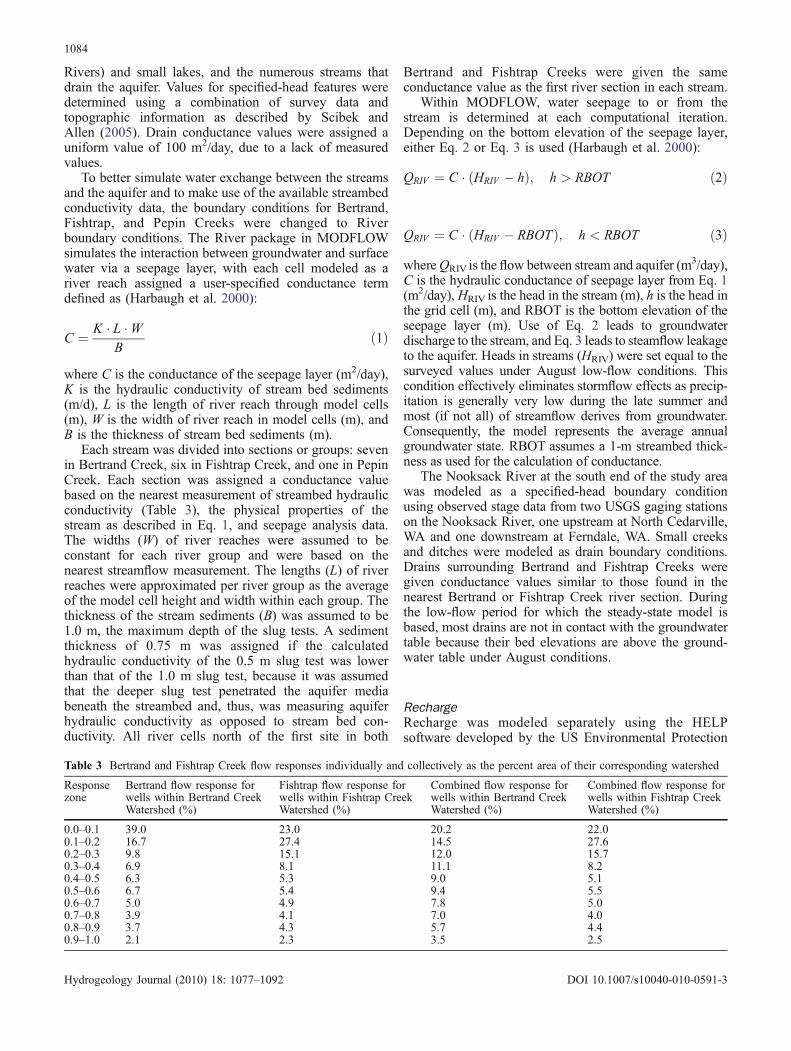
Table 3 Bertrand and Fishtrap Creek flow responses individually and collectively as the percent area of their corresponding watershed

Responsezone

Bertrand flow response forwells within Bertrand CreekWatershed (%)

Fishtrap flow response forwells within Fishtrap CreekWatershed (%)

Combined flow response forwells within Bertrand CreekWatershed (%)

Combined flow response forwells within Fishtrap CreekWatershed (%)

0.0–0.1 39.0 23.0 20.2 22.00.1–0.2 16.7 27.4 14.5 27.60.2–0.3 9.8 15.1 12.0 15.70.3–0.4 6.9 8.1 11.1 8.20.4–0.5 6.3 5.3 9.0 5.10.5–0.6 6.7 5.4 9.4 5.50.6–0.7 5.0 4.9 7.8 5.00.7–0.8 3.9 4.1 7.0 4.00.8–0.9 3.7 4.3 5.7 4.40.9–1.0 2.1 2.3 3.5 2.5

1084

Hydrogeology Journal (2010) 18: 1077–1092 DOI 10.1007/s10040-010-0591-3

Agency (Schroeder et al. 1994). For this reason, rechargewas not considered a calibration variable. HELP solves aseries of soil–water balance equations for a layeredcolumn of material using a time series of meteorologicaldata as input to the top of the model. HELP accounts forthe effects of surface storage, runoff, evapotranspiration,snowmelt, infiltration, vegetation growth, soil moisturestorage, lateral subsurface drainage, unsaturated verticaldrainage, and leakage through soil. Detailed descriptionsof all inputs and equations can be found in the supportingdocumentation for HELP (Schroeder et al. 1994). Slopecan be incorporated (quasi two-dimensional); however, thesimulation is one-dimensional. For recharge simulations,the base of the column is set equal to the depth of thewater table, and leakage simulated through the bottom ofthe soil column is considered representative of directrecharge to the groundwater system. To account for spatialvariability, recharge was simulated for different rechargezones (Scibek and Allen 2006); each zone representedunique combinations of soil media type, shallow aquiferpermeability, and depth to water table. In total, 64different recharge zones were modeled. Recharge wasthen applied to the top active layer of the groundwaterflow model.

To assure that the average annual recharge values in themodel (based on 30-year historical climate data) arerepresentative of 2006 field data, annual precipitation for2006 at Clearbrook, WA (approximately 14 km from thestudy site; National Climate Data Centre 2007a) wascompared to the normal precipitation observed since theyear 1919 (National Climate Data Centre 2007b). For2006, a total of 1,139 mm of rain was recorded, whichamounted to only 23 mm less than normal. This departurefrom normal was insignificant, and therefore no attemptwas made to adjust the recharge values previously definedby Scibek and Allen (2006).

Pumping wellsThe original model by Scibek and Allen (2005) includedonly selected pumping wells from the Washington StateDepartment of Ecology’s well log database. Whencombined, the wells within the Bertrand WatershedImprovement District (WID) totaled a pumping rate of138 l/s. According to Wubbena et al. (2004), approx-imately 3,000 ha within the Bertrand WID requireapproximately 1,379 l/s of groundwater during the monthof July for irrigation purposes. Similar demands wereassumed to be applicable in August.

To determine pumping rates, a water right databasedeveloped by the Public Utilities District 1 Water RightsTeam for the Water Resource Inventory Area (WRIA) 1Watershed Management Project was used to importgroundwater rights, certificates, and claims into thegroundwater model. Because the estimated amount ofpumping did not match the sum of the permitted waterrights, all water rights were scaled equally to match theestimated groundwater irrigation use for the Bertrand

Watershed Improvement District as determined by Hydro-logic Services Company (Wubbena et al. 2004).

Model calibrationIn addition to the more than 1,000 existing observationwells input in the original model by Scibek and Allen(2006), six local monitoring wells (Fig. 3), along with anumber of USGS wells, were added to the groundwatermodel to serve as head observation points. For the entiremodel domain, the calibration of observed to measuredstatic water levels yielded a root mean squared (RMS)error of 10.0 m, with a normalized RMS error of 8.7% anda residual mean error of 3.5 m. The calibration statisticswere found to be similar to those of the original model ofScibek and Allen (2005), which were considered to bereasonable given the large scale of the model and limitednumber of observations. Moreover, the spatial distributionof residuals was generally good, although there werepockets where simulated heads were all higher or all lowerthan observed values.

Zone Budget (Harbaugh 1990) was used in VisualMODFLOW to calculate sub-regional water budgets fordifferent zones in the model and to verify the calibration.A total of 20 zones were created between locations ofmeasured streamflow: eight in Bertrand Creek, eight inFishtrap Creek, one in Pepin Creek, and three for majordrains. Only cells that were defined as river or drainboundaries were included in a zone. For each sub-regionalwater budget zone, the cell-by-cell budget results weretabulated. Beginning with known flows from EnvironmentCanada gaging stations at the USA-Canada border forBertrand, Fishtrap, and Pepin Creeks, the predicted gainsand losses from each river reach or zone were added to, orsubtracted from, the known flow to obtain a “corrected”flow (Table 1 values) and compared to our measured flowvalues to determine the accuracy of the model. It is notedthat the Stream package within Visual MODFLOW wouldhave accounted for the flows automatically, but the Riverpackage was chosen in order to preserve the surface waterhead values in the original model.

Locally, the calibration results pointed to some dis-crepancies between “corrected” and modeled streamflows.A comparison of the “corrected” and modeled flows forBertrand Creek (Fig. 4) and measured1 and modeled flowsfor Fishtrap Creek (Fig. 4) revealed that the model over-predicts streamflow in the area of site B-2, and slightlyover-predicts streamflow in the upper reaches of FishtrapCreek; however, the model closely matches the “cor-rected” flows in the lower reaches of Bertrand Creek andthe measured flows of Fishtrap Creek. A comparison ofthe observed and modeled hydraulic heads within the localstudy area (in the aquifer nearby Bertrand and FishtrapCreeks) yielded better statistics than the overall regionalmodel, with a RMS error of 3.1 m, a normalized RMSerror of 5.4%, and a residual mean error of 1.8 m.

1 Fishtrap Creek flows were not corrected as discussed previously.

1085

Hydrogeology Journal (2010) 18: 1077–1092 DOI 10.1007/s10040-010-0591-3

Response functionsResponse functions were manually created for each of 346hypothetical well locations (Fig. 5). Pumping wells wereadded to the calibrated steady-state groundwater flowmodel, one at a time, and the streamflow impacts wereobtained for each through the use of Zone Budget. Eachpumping well was given a screen interval of 9–13 mbelow the ground surface, and because response functionsare typically based on a unit stress, the wells wereassigned a pumping rate of 28.3 l/s—this is equivalent to1 cubic foot per second (cfs).

For each well location, a response ratio ranging from0.0 (no impact on stream) to 1.0 (completely taken fromstream) was determined for Bertrand Creek and FishtrapCreek as the change in modeled streamflow at eachcreek’s terminus with the Nooksack River divided by thepumping rate. As in Barlow et al. (2003) and Cosgroveand Johnson (2004), it was assumed the rate of streamflowdepletion at each constraint site was a linear function of

the pumping rate of each groundwater well. Due to theunconfined nature of the groundwater model, the declinein water level was assumed to be very small such thatlinearity could be approximated. Since a steady-stategroundwater model was used, the streamflow responsesrepresent a worst-case scenario, because the zones ofinfluence of the pumping wells are at a maximum understeady-state conditions.

Raster maps of the response ratios with a 100-m cellsize were created for each stream using natural neighborinterpolation in ArcGIS (ESRI 2007). Natural neighborinterpolation uses a subset of data points that surround aquery point and applies weights to them based on propor-tionate areas in order to interpolate a value (Sibson 1981).

Groundwater-surface water interaction toolThe mapped response zones were used to create agroundwater and surface-water interaction tool, wherebythe user can replace surface-water use with a groundwaterpumping well of the same withdrawal rate, and determinethe streamflow impact for Bertrand and Fishtrap Creeks attheir terminus with the Nooksack River. STELLA version9.0.3 by isee Systems (2007) was chosen as the modelingenvironment for the interaction tool. The users can choosebetween four regions of interest within the study area, andthen select one of four sub-regions within that chosen region(Fig. 6). Upon choosing a sub-region, the user can easilylocate the location of a surface-water intake, and determinethe best location for a replacement groundwater well.

Overlain on the sub-region maps are the mappedresponse function zones for Bertrand and Fishtrap Creeks.The user identifies the Bertrand Creek response zone andthe Fishtrap Creek response zone for which the desiredreplacement groundwater well is located, and enters avalue for the surface-water withdrawal rate to be replacedby the groundwater well. Using the response functions

15000

20000

25000

30000C

reek

Flo

w(m

/day

)3

Bertrand Cr. Corrected Flow

Bertrand Cr. Modeled Flow

Fishtrap Cr. Measured Flow

Fishtrap Cr. Modeled Flow

0

5000

10000

1 2 3 4 5 6 7 8

WSU Gaging Station

Fig. 4 A comparison of corrected and modeled streamflows forBertrand and Fishtrap Creeks

NOO

K

SACK RIVE RBE

RTR

A

N

D C

RE

EK

F IS

H

TRAP CREEK

PE

PIN

CR

EE

K

CanadaUSA

0 1 20.5 Kilometers

Modeled Well

Fig. 5 Modeled well locations for determination of response ratios

1086

Hydrogeology Journal (2010) 18: 1077–1092 DOI 10.1007/s10040-010-0591-3

and the provided user input, the STELLA model comparesthe streamflow values for Bertrand and Fishtrap creeks foreach of a surface-water replacement well and a surface-water use. The impact on each creek is determined as thedifference between those two sets of flow values. The usermay, through trial-and-error, select the best option.

Results

Maps of the response functions for each of Bertrand Creekand Fishtrap Creek are shown in Figs. 7 and 8,

respectively, based on an independent modeling assess-ment of each. Response functions for each well locationranged from 0 to 1.0; these were contoured and classedinto five categories. Table 3 presents the Bertrand andFishtrap Creek flow responses, respectively, as the percentarea of their corresponding watershed. Seventy-ninepercent of the Bertrand Creek watershed and 79% of theFishtrap Creek watershed have response ratios less than0.5.

Because a steady-state model was used to generatethe response functions, it is important to consider whatthe other sources of water are to each pumping well.

Fig. 6 Screen shot of the STELLA interactive tool. Colors represent ranges of response functions: red (0.8–1.0), orange (0.6–0.8), yellow(0.4–0.6), light green (0.2–0.4), green (0–0.2)

NOOKSAK R.

BER

TRAN

DC

R.

FISHTRAP CR.

PE

PIN

CR

EE

K

CanadaUSA

0 1 20.5 Kilometers

Response Ratio

0.0 - <0.20.2 - <0.40.4 - <0.60.6 - <0.80.8 - 1.0

Fig. 7 Raster map of Bertrand Creek response ratios

1087

Hydrogeology Journal (2010) 18: 1077–1092 DOI 10.1007/s10040-010-0591-3

There are four potential sources of water to eachpumping well simulated: (1) streamflow-from one ofthe three main streams simulated as River boundaries,(2) seepage from the drain cells used to represent thesmaller tributary streams, (3) seepage from the NooksakRiver, which was defined as a specified head boundarycondition, and (4) recharge applied to the top surface ofthe model (mean annual recharge). As noted previously,during the low-flow period, most drains cells are not incontact with the groundwater table because their bedelevations are above the groundwater table under Augustconditions. Therefore, generally, the small streams do notact as a source of water to the wells. For wells inproximity to the Nooksak River, some of the water mayderive from this source, but as the impact on the mainstreams was of interest, this source was not considered.Therefore, apart from water derived from the majorstreams, the only other source is recharge. The calculatedresponse functions are non-uniformly distributed asshown in Figs. 7 and 8. For areas with low responseratios such as the lower area between Bertrand andFishtrap Creeks just above the confluence with theNooksak, the wells are far enough from either creek todraw water from them, and recharge is the source. Forwells near the Nooksak River below Fishtrap Creek,some water derives from that river.

The results suggest that pumping wells placed east ofFishtrap Creek essentially have no discernable impact onBertrand Creek. Similarly, pumping wells placed west ofBertrand Creek have almost no discernable impact onFishtrap Creek. Because groundwater movement occursacross the watershed boundaries, groundwater pumpingwells located in the area between Bertrand and Fishtrap

Creeks can impact streamflows in both creeks. Also, thereare reaches where groundwater pumping has less impacton the streamflow on one side of the creek as opposed tothe other. From a practical perspective, a surface-waterreplacement well should not be allowed to benefit onecreek while harming the other.

To better illustrate the overall response functions, acombined response ratio interpolation map was created byadding the Bertrand Creek and Fishtrap Creek responsesfor each well location (Fig. 9). Table 3 also shows thecombined flow response for Bertrand and Fishtrap Creeksas the percent area of their corresponding watershed.Sixty-seven percent of the Bertrand Creek watershed and79% of the Fishtrap Creek watershed have combinedresponse ratios less than 0.5, indicating highly favorableexchange opportunities.

Despite the favorable conditions for replacement ofsurface water use by groundwater pumping wells in over77% of the study area, internal testing of the STELLAinterface suggested that it might not be economicallypractical for farmers to replace their surface-water sourcefor a groundwater withdrawal if they have to construct alengthy pipeline to transport water to their field. Con-sequently, streamflow responses from wells located withinnarrow bands of both streams were specifically examined.Of the area within a 0.8-km band of Bertrand Creek, 57%has a combined flow response ratio less than 0.5, andwithin a 1.6-km band, 64% has a combined flow responseratio less than 0.5 (Table 4). Of the area within a 0.8-kmband of Fishtrap Creek, 70% has a combined flowresponse ratio less than 0.5, and within a 1.6-km band,77% has a combined flow response ratio less than 0.5(Table 4).

Fig. 8 Raster map of Fishtrap Creek response ratios

1088

Hydrogeology Journal (2010) 18: 1077–1092 DOI 10.1007/s10040-010-0591-3

Discussion

Simulation results suggested that replacing surface-watersources with groundwater pumping wells may be a viablealternative for improving summer streamflows. It is clearthat pumping wells do impact Bertrand and Fishtrap Creekflows, but if placed within zones of a low response ratio,less impact would occur than removing an equivalentamount of water directly from the stream.

For each stream (Figs. 7 and 8) and for the combinedstream network (Fig. 9), areas where the response ratio ishigh (i.e., above 0.6) are proximal to the stream. However,the response ratios are not uniform along the stream lengthas might be expected if they were solely a function ofdistance to the stream and the pumping rate. Rather,variations in the spatial distribution of response ratiosappear to be correlated with spatial variations in thehydraulic conductivity within the model layer containing

the screened interval of the pumping well. Thus, surface-water replacement wells placed within zones with highhydraulic conductivity values will likely produce greaterresponses to the instream flows of Bertrand and Fishtrapcreeks.

The fact that the response ratios are not uniform alongthe stream length lends support for the use of a numericalgroundwater flow model over an analytical model for thistype of analysis. Analytical models cannot adequatelycapture the heterogeneity of the aquifer materials nor therange of stream bed conductance values and streamphysical properties. Numerical models generally have thisability provided there is sufficient information with whichto construct the model.

While the numerical groundwater flow model used inthis study was constructed at the regional scale, it doescapture a reasonable amount of heterogeneity in bothspatial recharge and geology (Scibek and Allen 2005) as

Table 4 Bertrand and Fishtrap Creek combined flow response as the percent area within 0.8 km and 1.6 km of Bertrand and FishtrapCreeks

Responsezone

Combined flow response forwells within 0.8 km ofBertrand Creek (%)

Combined flow response forwells within 1.6 km ofBertrand Creek (%)

Combined flow response forwells within 0.8 km ofFishtrap Creek (%)

Combined flow Response forwells within 1.6 km ofFishtrap Creek (%)

0.0–0.1 17.9 17.9 19.5 21.10.1–0.2 14.1 14.9 19.4 24.40.2–0.3 11.4 12.4 13.2 15.10.3–0.4 7.4 10.0 10.3 10.20.4–0.5 6.1 8.6 8.0 6.00.5–0.6 9.2 10.2 8.4 5.80.6–0.7 7.7 7.7 7.4 5.30.7–0.8 7.6 7.2 5.5 4.50.8–0.9 10.3 6.5 4.7 4.20.9–1.0 8.4 4.5 3.8 3.4

Fig. 9 Combined raster interpolation of Bertrand and Fishtrap Creek response ratios using a natural neighbor technique

1089

Hydrogeology Journal (2010) 18: 1077–1092 DOI 10.1007/s10040-010-0591-3

evidenced by the good calibration results both for streamflow and hydraulic head in the aquifer. While theadditional field data incorporated into the original ground-water flow model provided improved local detail, calibra-tion results suggested that additional research and datacollection could be used to further improve modelcalibration locally. Specifically, it is suggested that theoverestimation of river leakage in the upper reaches ofboth creeks may be due to non-permitted wells that wereunaccounted for, uncertainty in stream elevations, lowerhydraulic conductivity of the aquifer materials in thoseareas, or a combination of these factors.

Finally, there are three main limitations to this study.First, accurate knowledge of how much water is beingwithdrawn from both creeks for irrigation and how muchgroundwater is being pumped in the surrounding area iscrucial and is currently lacking. This situation is notuncommon in most watersheds and points to the need forongoing accounting of water use. Second, transient effectswere not evaluated in this study despite the fact that atransient model has been developed and used for climatechange impacts assessment (Scibek and Allen 2006). Atransient groundwater model would have provided greaterinformation on lag times between pumping and streamimpacts; however, this route was not taken partly due tothe paucity transient calibration data-additional long-termmonitoring wells are needed to improve on transientmodel calibration-and partly because it would be difficultto implement transient response functions into a STELLAmodel. Our choice of a steady-state model essentiallyprovides a maximum impact of pumping wells at a time ofthe year when streamflow would be most impacted.

Third, and perhaps most importantly, a groundwaterflow code was used rather than a coupled groundwater-surface water code, such as MIKE SHE (DHI 2009). Suchcodes, although highly parameterized, have the potentialto simulate the exchange of water between the surfacewater system and the groundwater system more accuratelythan a groundwater flow code. In MODFLOW, the river orspecified head boundary conditions, as were used in themodel for this study, assume that the head in the stream willremain at some specified level for the duration of thesimulation, regardless of how much water is extracted fromthe surrounding aquifer. Clearly, this could represent asignificant limitation to determining stream response func-tions, particularly under low-flow conditions. However,because simulations represented the replacement of surfacewater use with groundwater, there would be no change inthe stream width or depth (i.e., there is no net change instreamflow). However, if stream response functions are usedto assess new groundwater abstraction, then if the pumpingrates are relatively low and the effect of individual wellspumping does not lower the stream stage appreciably, theapproach is reasonable. Where the approach will begin tofall apart is when the cumulative effects of pumping areconsidered and where these cumulative effects result in alowering of the stream stage. This, of course, is more likelythe real situation and one that demands a more rigorouscoupled surface-water/groundwater model.

Finally, the STELLA interface was not rigorously testedin this study. This interface was developed specifically forWhatcom County as a means to assess what the potentialimpact on streamflow would be if surface-water sourceswere replaced with equivalent groundwater extractionwells. Nonetheless, decision support systems for watermanagers clearly offer a means to make informed decisionswithout the need for expert knowledge. For problemsinvolving groundwater and surface water, such tools havethe potential to be very valuable if the supporting modeloutcomes have themselves been reasonably determinedthrough scientific methods.

Conclusions

Groundwater and surface-water interactions are prominentwithin the Bertrand and Fishtrap Creek watersheds basedon measured responses of streamflow and groundwaterlevels as well as modeling results. Summer low flows inthese streams are currently at levels to jeopardize endan-gered and threatened fish habitat. Hence, an innovativeconjunctive management scheme is needed.

This study investigated the replacement of surface-water sources with groundwater withdrawals using anumerical groundwater flow model. Response ratios,calculated from the modeled change in streamflow dividedby the pumping rate, were used to assess the impact onstreamflow of exchanging a surface-water source with agroundwater pumping well, based on the groundwaterflow model under steady state. Resulting response ratiosranged from 0 to 1, with 0 representing no impact on thestream and 1 representing an impact equivalent to that of asurface-water withdrawal at the same pumping rate. Themodel demonstrated that the greatest values occurred inclose proximity to the creeks and in areas with highhydraulic conductivity. For areas with low responsefunctions, the balance of water derived from precipitationrecharge or, for wells near the Nooksak River, from thatriver source.

Simulation results suggest that replacing surface-watersources with groundwater pumping wells may be a viablealternative for improving summer streamflows. It is clearthat pumping wells do impact Bertrand and Fishtrap Creekflows, but if placed within zones of a low response ratio,less impact would occur than removing an equivalentamount of water directly from the stream. Within a 1.6-kmdistance on either side of the stream, 64% of BertrandCreek had combined response ratios less than 0.5, whilewithin the same distance, 77% of Fishtrap Creek hadcombined response ratios less than 0.5, indicating highlyfavorable exchange opportunities for both creeks.

Because MODFLOW is difficult to understand andoperate for non-specialists, response functions werecreated and, by using the STELLA software, a user-friendly interface was created through which users canlearn about groundwater and surface-water interactionswithin the study area. The STELLA model provides aquick and easy estimation of the streamflow impacts on

1090

Hydrogeology Journal (2010) 18: 1077–1092 DOI 10.1007/s10040-010-0591-3

Bertrand and Fishtrap Creeks without the need to re-runthe groundwater flow model.

Acknowledgements This research was funded by the Departmentof Public Works, Whatcom County, Washington through a grant tothe State of Washington Water Research Center. We thank HenryBierlink and Karen Steensma for their knowledge on the study areaand assistance in gaining land access, as well as all landowners whopermitted access to their land for this research and Erin Moilanenfor her assistance in developing the visual analysis tool.

References

Adelsman H (2003) Washington water acquisition program findingwater to restore streams. Publ. 03-11-005, Washington StateDepartment of Ecology, Olympia, WA, 136 pp. http://www.ecy.wa.gov/biblio/0311005.html. Cited January 2010

Allen DM, Chesnaux R, McArthur S (2007) Nitrate transportmodeling within the Abbotsford-Sumas Aquifer, British Colum-bia, Canada and Washington State, USA. Department of EarthSciences, Simon Fraser University, Burnaby, BC, 181 pp

Armstrong JE, Crandell DR, Easterbrook DJ, Noble JB (1965) LatePleistocene stratigraphy and chronology in southwestern BritishColumbia and northwestern Washington. Geol Soc Am Bull76:321–330

Barlow PM, Ahlfeld DP, Dickerman DC (2003) Conjunctive-management models for sustained yield of stream aquifersystems. J Water Resour Plan Manage 129(1):35–48

Berg MA, Allen DM (2007) Low flow variability in groundwater-fed streams. Can Water Resour J 32(3):227–245

Boyle CA, Lavkulich L, Schreier H, Kiss E (1997) Changes in landcover and subsequent effects on lower Fraser Basin ecosystemsfrom 1827 to 1990. Environ Manage 21:185–196

Buchanan TJ, Somers WP (1969) Discharge measurements atgaging stations. In: Applications of hydraulics, US Geol SurvTech Water Resour Invest, Chap. A8, Book 3, US GeologicalSurvey, Reston, VA, 65 pp. http://pubs.usgs.gov/twri/twri3a8/.Cited January 2010

Chen X, Chen X (2003) Stream water infiltration, bank storage, andstorage zone changes due to stream-stage fluctuations. J Hydrol280:246–264

Cooper HH, Rorabaugh MI (1963) Groundwater movements andbank storage due to flood stages in surface streams. US GeolSurv Water Suppl Pap 1536-J:343–366

Cosgrove DM, Johnson GS (2004) Transient response functions forconjunctive water management in the Snake River Plain, Idaho.J Am Water Resour Assoc 40(6):1469–1482

Cox SE, Kahle SC (1999) Hydrogeology, ground-water quality, andsources of nitrate in lowland glacial aquifers of WhatcomCounty, Washington, and British Columbia, Canada. US GeolSurv Water Resour Invest Rep 98-4195

Cox SE, Simonds FW, Doremus L, Huffman RL, Defawe RM (2005)Ground water/surface water interactions and quality of discharg-ing ground water in streams of the Lower Nooksack River Basin,Whatcom County, Washington. US Geol Surv Sci Invest Rep2005-5225, 56 pp. http://pubs.usgs.gov/sir/2005/5255/. CitedJanuary 2010

Culhane T (1993) Whatcom County hydraulic continuity investiga-tion-part 1, critical well/stream separation distances for minimiz-ing stream depletion. Open File Technical Report 93-08,Washington State Department of Ecology, Olympia, WA, 20pp. http://www.ecy.wa.gov/biblio/9308.html. Cited January 2010

DHI (2009) MIKE SHE modeling software. DHI, Hørsholm,Denmark. http://www.dhigroup.com/Software/WaterResources/MIKESHE.aspx. Cited January 2010

ESRI (2007) GIS and mapping software. ESRI, Redlands, CA.http://www.esri.com/. Cited January 2010

Hamilton TS, Ricketts BD (1994) Contour map of the sub-Quaternary bedrock surface, Strait of Georgia and Fraser

Lowland. In: Monger JWH (ed) Geology and geologicalhazards of the Vancouver region, southwestern British Colum-bia. Geol Surv Can Bull 481:193–196

Hantush MM (2005) Modeling stream-aquifer interactions withlinear response functions. J Hydrol 311:59–79

Harbaugh AW (1990) A computer program for calculating subre-gional water budgets using results from the U.S. GeologicalSurvey modular three-dimensional ground-water flow model.US Geol Surv Open-File Rep 90-392, 46 pp

Harbaugh AW, Banta ER, Hill MC, McDonald MG (2000)MODFLOW-2000, the U.S. Geological Survey modularground-water model: user guide to modularization conceptsand the ground-water flow process. US Geol Surv Open-FileRep 00-92. http://water.usgs.gov/nrp/gwsoftware/modflow2000/ofr00-92.pdf. Cited January 2010

isee Systems (2007) STELLA, version 9.0.3. isee Systems, Lebanon,NH, http://www.iseesystems.com/. Cited January 2010

Jenkins CT (1968a) Techniques for computing rate and volume ofstream depletion by wells. Ground Water 6(2):37–46

Jenkins CT (1968b) Computation of rate and volume of streamdepletion by wells. In: Hydrologic analysis and interpretation,Chap. D1, Book 4, , Tech Water Resour Invest, US GeologicalSurvey, Reston, VA, 21 pp. http://pubs.usgs.gov/twri/twri4d1/.Cited January 2010.

Leake SA, Reeves HW (2008) Use of models to map potentialcaptures of surface water by ground-water withdrawals. In:Proceedings of MODFLOW and More: Ground Water andPublic Policy, The Colorado School of Mines, Golden, CO,USA, 18–21 May 2008, pp 204–208

Leake SA, Green W, Watt D, Weghorst P (2008a) Use ofsuperposition models to simulate possible depletion of ColoradoRiver water by ground-water withdrawal. US Geol Surv SciInvest Rep 2008-5189, 25 pp

Leake SA, Pool DR, Leenjouts JM (2008b) Simulated effects ofground-water withdrawals and artificial recharge on discharge tostreams, springs, and riparian vegetation in the Sierra VistaSubwatershed of the Upper San Pedro Basin, southeasternArizona. US Geol Surv Sci Invest Rep 2008-5207, 14 pp

Kemblowski M, Asefa T, Haile-Selassje S (2002) Ground waterquantity report for WRIA 1, Phase II. WRIA 1 WatershedManagement Project., US Geological Survey, Reston, VA,http://wa.water.usgs.gov/projects/wria01/. Cited January 2010

Maddock III T, Lacher LJ (1991) MODRSP: A program to calculatedrawdown, velocity, storage, and capture response functions formulti-aquifer systems. Report No. HWR 91-020, Dept. ofHydrology and Water Resources, University of Arizona,Tucson, AZ

McKenzie C (2007) Measurements of hydraulic conductivity usingslug tests in comparison to empirical calculations for twostreams in the Pacific Northwest, USA. MSc Thesis, Wash-ington State University, USA

Mitchell RJ, Babcock RS, Gelinas S, Nanus L, Stasney DE (2003)Nitrate distributions and source identification in the Abbotsford-Sumas Aquifer, northwestern Washington. J Environ Qual 32(3):789–800

Moench AF, Barlow PM (2000) Aquifer response to stream-stageand recharge variations. I. Analytical step-response functions. JHydrol 230:192–210

Morel-Seytoux HJ (1975) A combined model of water table andriver stage evolution. Water Resour Res 11(6):968–972

National Climatic Data Center (2007a) 2006 and 2007 hourlyprecipitation data for Bellingham International Airport, WA.NOAA, Silver Spring, MD. http://cdo.ncdc.noaa.gov/qclcd/QCLCD?prior=N. Cited January 2010

National Climatic Data Center (2007b) 2006 annual climatologicalsummary for Clearbrook, WA. NOAA, Silver Spring, MD.http://www7.ncdc.noaa.gov/CDO/cdo. Cited January 2010

Perkins SP, Koussis AD (1996) Stream-aquifer interaction modelwith diffusive water routing. J Hydraul Eng 122(4):210–218

Pinder GF, Sauer SP (1971) Numerical simulation of flood wavemodification due to bank storage effects. Water Resour Res 7(1):63–70

1091

Hydrogeology Journal (2010) 18: 1077–1092 DOI 10.1007/s10040-010-0591-3

Pruneda EB (2007) Use of stream response functions and STELLAsoftware to determine impacts of replacing surface waterdiversions with groundwater pumping withdrawals on instreamflows within the Bertrand Creek and Fishtrap Creek watersheds,Washington State, USA. MSc Thesis, Washington State Uni-versity, USA, 70 pp

Saquillace PJ (1996) Observed and simulated movement of bank-storage water. Ground Water 34(1):121–134

Schroeder PR, Dozier TS, Zappi PA, McEnroe BM, Sjostrom JW,Peyton RL (1994) The hydrologic evaluation of landfillperformance (HELP) model: engineering documentation forversion 3. EPA/600/R-94/168b, US EPA, Washington, DC

Scibek J, Allen DM (2005) Numerical groundwater flow model ofthe Abbotsford-Sumas Aquifer, central Fraser lowland of BC,Canada, and Washington State, US. Department of EarthSciences, Simon Fraser University, Burnaby, BC

Scibek J, Allen DM (2006) Comparing modelled responses of twohigh permeability, unconfined aquifers to predicted climatechange. Global Planet Change 50:50–62

Sharp MJ (1977) Limitations of bank-storage model assumptions. JHydrol 35:31–47

Sibson R (1981) Interpolating multivariate data. Wiley, New York,pp 21–36

WAC 173-501-030 (1985) Establishment of instream flows.Washington State Legislature, Olympia, WA. http://apps.leg.wa.gov/WAC/default.aspx?cite=173-501-030. Cited January2010

Waterloo Hydrogeologic (2000) Visual MODFLOW v 3.0 usermanual. Waterloo Hydrogeologic, Waterloo, ON, Canada

Waterloo Hydrogeologic (2006) Visual MODFLOW v. 4.1 user’smanual. Waterloo Hydrogeologic, Waterloo, ON, Canada

Welch K, Willing P, Greenberg J, Barclay M (1996) NooksackRiver Basin pilot low flow investigation. Water ResourcesConsulting Team and Cascades Environmental Services, Portland,OR

Winter TC, Harvey JW, Franke OL, Alley WM (1998) Ground andsurface water a single resource. US Geol Surv Circ 1139, 79 pp.http://pubs.usgs.gov/circ/circ1139/. Cited January 2010

Wubbena R, Powell R, O’Rourke K et al (2004) Bertrand Water-shed Improvement District comprehensive irrigation districtmanagement plan. Economic and Engineering Services, Bellvue,WA

1092

Hydrogeology Journal (2010) 18: 1077–1092 DOI 10.1007/s10040-010-0591-3