UNLV Theses, Dissertations, Professional Papers, and Capstones

8-1-2012

Analysis of Bank Failure and Size of AssetsGuancun ZhongUniversity of Nevada, Las Vegas, zhongg@unlv.nevada.edu

Follow this and additional works at: https://digitalscholarship.unlv.edu/thesesdissertations

Part of the Analysis Commons, Applied Statistics Commons, Economic Policy Commons,Finance Commons, and the Finance and Financial Management Commons

This Thesis is brought to you for free and open access by Digital Scholarship@UNLV. It has been accepted for inclusion in UNLV Theses, Dissertations,Professional Papers, and Capstones by an authorized administrator of Digital Scholarship@UNLV. For more information, please contactdigitalscholarship@unlv.edu.

Repository CitationZhong, Guancun, "Analysis of Bank Failure and Size of Assets" (2012). UNLV Theses, Dissertations, Professional Papers, and Capstones.1702.https://digitalscholarship.unlv.edu/thesesdissertations/1702

 

ii 

ANALYSIS OF BANK FAILURE AND SIZE OF ASSETS

by

Guancun Zhong

Master of Science Dalian University of Technology

2009

A thesis submitted in partial fulfillment of the requirements for the

Master of Science in Mathematical Sciences

Department of Mathematical Sciences College of Sciences Graduate College

University of Nevada, Las Vegas August 2012

 

ii 

 

 

 

 

 © Copyright by Guancun Zhong 2012

All Rights Reserved  

 

 

 

 

 

 

 

 

 

 

ii 

THE GRADUATE COLLEGE We recommend the thesis prepared under our supervision by Guancun Zhong entitled Analysis of Bank Failure and Size of Assets be accepted in partial fulfillment of the requirements for the degree of Master of Science in Mathematical Sciences Department of Mathematical Sciences Chih-Hsiang Ho, Committee Chair Kaushik Ghosh, Committee Member Amei Amei, Committee Member Hualiang Teng, Graduate College Representative Tom Piechota, Ph.D., Interim Vice President for Research & Dean of the Graduate College August 2012

 

iii  

ABSTRACT

Analysis of Bank Failure and Size of Assets

by

Guancun Zhong

Dr. Chih-Hsiang Ho, Examination Committee Chair Professor of Mathematical Sciences

University of Nevada, Las Vegas

The financial health of the banking industry is an important prerequisite for

economic stability and growth. Bank failures in the United States have run in cycles

largely associated with the collapse of economic bubbles. The number of bank failures

has increased dramatically over the last thirty years (Halling and Hayden, 2007). In this

thesis, we try to address the following two questions: 1) What is the relationship, if any,

between a bank’s asset size and its likelihood of failures? 2) How can we use statistical

tools to predict the numbers of bank failures in the future? Various modeling techniques

are proposed and applied to bank failure data from Federal Deposit Insurance

Corporation. For the first question, we find that there is a relationship between bank size

and bank failure status based on the Pearson’s chi-square test. To answer the second

question, first, logistic regression is applied to the bank failure data, and the

corresponding prediction rule and prediction results are obtained. Second, we develop the

empirical recurrence rate (Ho, 2008) and empirical recurrence rates ratio time series for

 

iv  

the given data, and also perform corresponding theoretical and graphical analysis on both

of them. We obtained much valuable information on the reason for, time period of, and

trends of bank failures in the past thirty years. We perform pairwise bank failure rate

comparisons using the conditional test (Przyborowski and Wilenski, 1940). Additionally,

based on the smooth behavior of empirical recurrence rate and empirical recurrence rates

ratio time series, we apply autoregressive fractional integrated moving average models to

both of the series for forecasting purposes. Finally, some interesting results are discussed.

 

v  

ACKNOWLEDGEMENTS

A few words of thanks seem inadequate to express my appreciation for those who

have helped me over the past years. First of all, I would like to say thank you to my

advisor, Dr. Chih-Hsiang Ho; his encouragement and guidance are invaluable. His

excellence in both research and teaching will always be a great example to me.

I am indebted to many individuals who have directly and indirectly supported me in

this work, including these respectful committee members: Dr. Amei Amei, Dr. Kaushik

Ghosh and Dr. Hualiang Teng, for their positive inputs and mentoring during my

graduate studies.

Last but not the least, I am eternally grateful to my family for their love, support and

understanding, which strengthened me to accomplish this study.

 

 

 

 

 

 

 

 

 

 

vi  

CONTENTS

ABSTRACT…………………………………………………………………………………………………..……..…………………iiii 

ACKNOWLEDGEMENTS…………………………………………………………………………………….…….………….v 

LIST OF TABLES…………………………………………………………………………………………………….….………..viii 

LIST OF FIGURES……………………………………………………………………………………………………….………….ix 

CHAPTER 1 INTRODUCTION……………………………………………………………………………….……...………1 

CHAPTER 2 EXPLORATORY DATA ANALYSIS……………………………………………………….…..…..4 

2.1 Data……………………………………………………………………………………………………………..……..…..………4 

2.1.1 CPI adjustment…………………………………………………………………………………………….…..……….5 

2.1.2 Bank classification…………………………………………………………………………………….………..…….5 

2.2 Pearson's chi-square test for independence…………………………………………………………….…………8 

2.3 Relative risk and odds ratio………………………………………………………………………………….…………..9 

CHAPTER 3 LOGISTIC REGRESSION……………………………………………………………………….……….13 

3.1 Methodology………………………………………………………………………………………………….…….………..13 

3.1.1 Simple logistic regression……………………………………………………………………….…….…………13 

3.1.2 Maximum likelihood estimation……………………………………………………………….…….……….13 

3.2 Modeling…………………………………………………………………………………………………………….…….……15 

3.2.1 Application and interpretation………………………………………………………………………………...15 

3.2.2 ROC curve and prediction on new observations………………………………………………….…..17 

CHAPTER 4 GRAPHICAL ANALYSIS……………………………………………………………………………..….22 

4.1 Empirical recurrence rate………………………………………………………………………………………….……22 

4.2 Empirical recurrence rate plots……………………………………………………………………..………………..22 

4.3 Pairwise comparisons……………………………………………………………………………………..………………26 

4.3.1 Conditional test……………………………………………………………………………………………….………26 

4.3.2 Application………………………………………………………………………………………………….………….28 

4.4 Empirical recurrence rates ratio………………………………………………………………………,….………….30 

4.5 Empirical recurrence rates ratio plots……………………………………………………………………..………31 

CHAPTER 5 ARIMA AND ARFIMA MODELING………………………………………………………..……..39 

 

vii  

5.1 Autoregressive integrated moving average models…………………………………………….………….39 

5.2 Data transformation……………………………………………………………………………………………..………..41 

5.2.1 Box-Cox transformation……………………………………………………………………………..…………..41 

5.2.2 Differencing……………………………………………………………………………………………………..……..42 

5.3 Autoregressive fractional integrated moving average models……………………………….………..43 

5.4 Model diagnostics………………………………………………………………………………………………………..…44 

5.4.1 Sample ACF/PACF of the residuals………………………………………………………………..……….44 

5.4.2 Tests for randomness of the residuals…………………………………………………………..………….44 

CHAPTER 6 APPLICATION……………………………………………………………………………………..…………..47 

6.1 Modeling for ERR time series……………………………………………………………..…………………………47 

6.2 Modeling for ERRR time series………………………………………..…………………………………………..57 

6.3 Full data set prediction……………………………………………………………………………………….………….64 

CHAPTER 7 CONCLUSIONS……………………………………………………………………………….………………66 

APPENDIX І……………………………………………………………………………………………………….………………….68 

APPENDIX ІІ……………………………………………………………………………………………………..…………………..69 

BIBLIOGRAPHY…………………………………………………………………………………………………..……………….73 

VITA………………………………………………………………………………………………………………..……………………..75 

 

 

 

 

 

 

 

 

 

 

viii  

LIST OF TABLES

 

Table 1 Counts of banks by failure status and asset group during 1980:Q1 to 2011:Q4………...….6 

Table 2 Collapsed 2x2 contingency tables based on Table 1……………………………………….…………….9 

Table 3 Results of Pearson's chi-square tests for independence…………………………………………….…..9 

Table 4 Relative risk and odds ratio……………………………………………………………………………….………..10 

Table 5 Point estimator and 95% confidence interval for relative risk………………………………….….11 

Table 6 Point estimator and 95% confidence interval for odds ratio…………………………………….….12 

Table 7 Conditional tests for pairwise comparisons for H0: pij = 0.5, 1 ≤ i < j ≤ 4………………..…..29 

Table 8 Counts of bank failure by Status and Group for the second period (1996:Q1 to

aaaaaaaA2011:Q4)………………………….……………………………………………………………………………….………30 

Table 9 Conditional tests for pairwise comparisons – 1996 - 2011………………………………….………30 

Table 10 Numerical values of observed ERRs, observed counts in the prediction set, predicted

aaaaaaaAERRs (Using MA(4)) and corresponding predicted counts for the prediction set…..….56 

Table 11 Comparisons between real ERRRs of small-large bank failure comparison and its

aaaaaaaApredictions……………………………………………………………………………………………………….…..…..64

Table 12 Full data (1980:Q1 – 2011:Q4) time series (Z0, ..., Z4, R12, ..., R34) modeling and

aaaaaaaAforecasting for 2012:Q1 to 2012:Q4…………………………………………………………...……….65 

 

 

 

ix  

LIST OF FIGURES

 

Fig. 1. Number of bank failures from 1980:Q1 to 2011:Q4……………………………………..………………..4 

Fig. 2. Numbers of bank failures from 1980:Q1 to 2011:Q4 by groups…………………………….……….7 

Fig. 3. ROC curve for the logistic regression model fitted to bank failures from 1980:Q1 to

aaaaaa1995:Q4…………………………………………………………………………………………………………..…..………19 

Fig. 4. Plots of bank failures and ERRs……………………………………………………………………………..……23 

Fig. 5. ERR plots by groups…………………………………………………………………………………………….….….24 

Fig. 6. ERR plots by groups for the second period (1996:Q1 to 2011:Q4)………………………….…..26  

Fig. 7. ERRR plots for pairwise comparisons….………………………………………………………………….…..32 

Fig. 8. ERRR plots for pairwise comparisons for second period (1996:Q1 to 2011:Q4)……..……34 

Fig. 9. Plots of Rij vs. P (reference line) for all 1 = i < j = 4 during 1980:Q1 and 2011:Q4….....36 

Fig. 10. Plots of Rij vs. P (reference line) for all 1 = i < j = 4 during 1996:Q1 and 2011:Q4……37 

Fig. 11. ERR plots (Z3) with training sample and prediction set……………………………………..………47 

Fig. 12. a. Time plot; b. ACF; c. PACF of the training sample…………………………………………..……48 

Fig. 13. a. Time plot; b. ACF; c. PACF of the lag-1 differenced training sample…………..….…….49 

Fig. 14. a. Time plot; b. ACF; c. PACF of the twice differenced training sample…………..……….50 

Fig. 15. Diagnostics for the MA (5) fitted to the mean-corrected and twice differenced training

aaaaaaaasample. a. time plot, b. ACF, and c. PACF of the rediduals……………………………….………53 

Fig. 16. Diagnostics for the subset model of MA (5) fitted to the mean-corrected and twice

aaaaaaaadifferenced training sample. a. time plot, b. ACF, and c. PACF of the rediduals……...54 

Fig. 17. Diagnostics for MA (4) model fitted to the mean-corrected and twice differenced

aaaaaaaatraining sample. a. time plot, b. ACF, and c. PACF of the residuals……….…………………55 

Fig. 18. Comparison of the forecasted ERRs using MA (5), subset MA (5) and MA (4) model

aaaaaaaathe observed data……………………………..………………………………………………………..……………..56 

Fig. 19. ERRR plots (R23) with training sample and prediction set………………………..………………..57 

Fig. 20. a. Time plot; b. ACF; c. PACF of the training sample…………………………………..……………58 

Fig. 21. a. Time plot; b. ACF; c. PACF of the lag-1 differenced training sample………..…….…….59 

Fig. 22. Diagnostics for ARIMA(4,2) fitted to the mean-corrected and lag-1 differenced training

aaaaaaaasample. a. time plot, b. ACF, and c. PACF of the residuals ………………………….…………..61 

Fig. 23. Diagnostics for ARFIMA(1,0.498,1) fitted to the mean-corrected training sample. a.

aaaaaaaatime plot, b. ACF, and c. PACF of the residuals …………………………………………....………..62 

Fig. 24. Comparison of forecasted ERRRs with the prediction set using ARMA (4, 2) and

aaaaaaaaARFIMA (1, 0.4985, 1)………………………………………..……………………………………..……………63  

 

 

1  

CHAPTER 1

INTRODUCTION

A bank fails when it can no longer cover its obligations (liabilities) with its assets and

must file for bankruptcy. Washington Mutual (WaMu) failed on September 25, 2008.

WaMu reportedly had over $30 billion in assets at the time of their failure; almost 300

banks have collapsed since then. During the two years since WaMu failed, the number of

bank failures significantly increased compared to the previous six years, during which

period only around 40 banks failed. In retrospect, the number of bank failures has

increased dramatically over the last 25 years. Out of 3,879 total bank failures since 1934,

when the Federal Deposit Insurance Corporation (FDIC) was established, nearly 3000

occurred between 1985 and 2010. The increase in bank failures is typically accompanied

by high unemployment and reduced liquidity. Moreover, the survivors collect the market

power by reducing competition and potentially harming consumers in the future (Levin

and Coburn, 2011).

To reduce the risk of bank failures, the FDIC, which, since 1980, guaranteed to pay

the first $100,000 deposit in full to each account-holder if the bank failed, temporarily

raised the amount to $250,000 during the financial crisis in 2008. Additionally, Congress

passed the Emergency Economic Stabilization Act to assist the banking industry during

the financial crisis. The United States Treasury spent up to $700 billion to support

distressed assets from banks, which injected new capital into the banking system. Despite

the aforementioned events, the number of bank failures increased. As more and more

 

2  

analysts focus their attention on the banking industry, a widespread concern emerges:

Will the situation worsen in the future?

Most previous studies of bank failures rely on bank-level accounting data,

occasionally augmented with market-price data. These studies aim to develop models of

an early warning system for individual bank failures (Cole and Wu, 2009). Since the

1980s, studies have been conducted using mathematical programming-based on

discriminant analysis. Theoretical studies on mathematical programming-based

discriminant analysis were first conducted in the early 80s (Freed and Glover, 1981).

These studies focused mostly on the applicability of mathematical programming

techniques on discriminant analysis and their formulation (Glover, 1990). Also conducted

were evaluation of the results of applications of these models (Wallin and Sundgren,

1995). Additionally, studies aimed at developing new models which were compatible

with new mathematical programming-based discriminant analysis were also conducted,

while goal-programming and mixed-integer programming were applied to combine

discriminant analysis and data-envelopment analysis (Sueyoshi, 1999). Although there

are several models in different fields in the literature, there is a consensus on “minimum

sum of deviations model (MSD)” as the model which gives the most proper results in a

significant portion of studies (Karacabey, 2003).

In this thesis, we extend the work of Cui (2011) in a few ways: First, the time period

of data is different. Cui’s data starts from 1989, which is in the middle of Savings and

Loan crisis (1980s to 1990s). We extend that back to 1980, to include the entire Savings

and Loan crisis in our data. Second, different grouping strategies are applied; we separate

bank data into four equal groups using first quartile, median and third quartile of the

 

3  

adjusted assets, so we can hold the four population sizes the same. Third, we extend our

modeling method to ARFIMA to get a better prediction in the application part in Chapter

6.

Additionally, we use a two way contingency table to find the dependency of bank

status and bank size; We then perform simple logistic regression using adjusted assets as

the solo independent variable; Next we transfer the raw data to empirical recurrence rate

(ERR) and the empirical recurrence rates ratio (ERRR) time series, which is an extension

of ERR. We perform some detailed analysis and exploration on both ERR and ERRR.

Finally, we apply the autoregressive integrated moving average (ARIMA) and

autoregressive fractional integrated moving average (ARFIMA) models on ERR and

ERRR, including model selection, validation, and forecasting for the bank failures

classified by the total assets.

Specifically, bank data and Pearson’s chi-square tests are given in Chapter 2.

Logistic regression is presented in Chapter 3. Empirical recurrence rate (ERR) and

empirical recurrence rates ratio (ERRR) are introduced in Chapter 4. We have an

introduction to autoregressive integrated moving average (ARIMA) and autoregressive

fractional integrated moving average (ARFIMA) modeling in Chapter 5. In Chapter 6, we

predict the ERR and ERRR time series with ARIMA and ARFIMA models. Chapter 7

concludes our work.

 

4  

CHAPTER 2

EXPLORATORY DATA ANALYSIS

2.1 Data

The numbers of bank failures in the United States during 1980:Q1 to 2011:Q4 were

obtained from the FDIC (Federal Deposit Insurance Corporation) failed banks list

(http://fdic.gov/bank/individual/failed/banklist.html), which lists failed banks by name,

location, charter type, total assets, and other characteristics. We count the number of bank

failures on a quarterly basis. Based on this list, 3,212 banks were reported to fail over the

128 quarters (Fig. 1).

Fig. 1. Number of bank failures from 1980:Q1 to 2011:Q4.

0

50

100

150

200

250

Nu

mb

er o

f F

ailu

res

Quarters

Fig.1 Total US Bank Failures, 1980‐2011

 

5  

2.1.1 CPI adjustment

In economics, the nominal level of prices of goods and services changes over a

period of time. When the price level rises, each unit currency buys fewer amount of

goods and services. The purchasing power of money − the real value in the internal

medium of exchange and unit of account in the economy, changes over time. The

Consumer Price Index (CPI) is used to bridge nominal values to real values. The total

assets of banks are reported in terms of nominal price. To make the total assets in

different time periods comparable, the total assets of banks are converted to the real

values which are based on (Mankiw, 2002):

Adjustedtotalassets Totalassets ,

where Totalassets is the nominal total asset at time i (the month a failure was reported);

CPI is CPI at the ith month that bank failed; CPI is the CPI for the base month (taken as

January 2011 in this thesis).

2.1.2 Bank classification

The data on bank failures will be divided into four groups, based on the adjusted total

assets held by the banks at the time they failed. First, we have all bank assets adjusted by

CPI index and ordered from smallest to largest. Then, we set the banks with adjusted

assets (in millions) lower than the 1st quartile (67.43) of the adjusted assets list as our

“Small” banks group (also known as G1). Similarly, banks with adjusted assets between

1st quartile and the median (150) are referred to as “Medium” banks group (also known as

G2), banks with adjusted assets between median and 3rd quartile (360) are referred to as

“Large” banks group (also known as G3) and banks with adjusted assets higher than the

 

6  

3rd quartile are referred as “Grand” banks group (also known as G4). Counts of bank

failures by status (“Yes” for failed and “No” for solvent) and Group (1 through 4) are

summarized in Table 1. The time series plots by groups are illustrated in Fig. 2.

Table 1 Counts of banks by failure status and asset group during 1980:Q1-2011:Q4 Group

1 2 3 4

Totals[3.0, 67.4]* (67.4, 150] (150, 360] (360, 1810000]

Status Yes 1172 663 590 787 3212 No 1456 1965 2038 1841 7300

Totals 2628 2628 2628 2628 10512 * In millions

 

7  

Fig. 2. Numbers of bank failures from 1980:Q1 to 2011:Q4 by groups.

 

 

8  

2.2 Pearson's chi-square test for independence

We use Table 1 as a 2 x 4 contingency table and perform Pearson's chi-square test for

independence between Status and Group. The null hypothesis and alternative hypothesis

are stated as follows:

: Status and Group are independent.

: Status and Group are dependent.

The chi-square test statistic is 361.141 at 3 df, resulting in a p-value 0. Thus, we

conclude that the data provides sufficient evidence to reject the null hypothesis at a 5%

significance level. We conclude that there is an association between the failure status and

asset size of a bank.

We then collapsed Table 1 to produce four 2 x 2 contingency tables for G1 vs. the

rest, G2 vs. the rest, G3 vs. the rest and G4 vs. the rest with the same null hypotheses. The

corresponding contingency tables are given in Table 2 and the results are shown in Table

3. Testing each of the groups, G1, G2 and G3, against their corresponding complementary

groups results in rejection of corresponding at α = 0.05 leading us to conclude that

there is some type of dependence between group membership and failure status. Testing

G4 against all the other banks results in that there is not enough evidence to reject the null

hypothesis at α = 0.05. It appears that the “Group” partitioned by G4 and the others are

independent of “Status”. This means that whether a bank is “Grand” or not has no bearing

on its failure status.

\

 

9  

Table2 Collapsed 2x2 contingency tables based on Table 1

Group 1 Rest 2 Rest 3 Rest 4 Rest

Status Yes 1172 2040 663 2459 590 2622 787 2425 No 1456 5844 1965 5335 2038 5262 1841 5459

2.3 Relative risk and odds ratio

The relative risk (RR) is the risk of an event (bank failure) relative to exposure

(selected group). In other words, RR is a ratio of the probability of the event occurring in

the exposed group (Gi) versus a non-exposed group (all the other groups combined). Let

RRi be the relative risk of bank failures occurring in Gi (i = 1, 2, 3, 4) vs. all the other

groups combined (excluding Gi). In Table 4, F represents counts of failed banks and S is

for solvent banks.

Table 3 Results of Pearson's chi-square tests for independence

Pairwise comparisons 1 vs. Rest 2 vs. Rest 3 vs. Rest 4 vs. Rest

Test statistic 325.6 46.9 108.5 0.61 P-value 0 0 0 0.434

 

10  

Table 4 Relative risk and odds ratio

Group

i others

StatusYes Fi F. No Si S.

Then, we define RRi= /

./ . .,

The odds ratio (OR) is a measure of effect size, describing the strength of association

or non-independence between two binary data values. Unlike the relative risk, the odds

ratio treats the two variables being compared symmetrically, and can be estimated using

some types of non-random samples (Sistrom and Garvan, 2004). For odds ratio, we first

define odds for Gi by

ω π 1 π⁄ , where π = Prob (bank failure for Gi). Similarly, we define “ω∙” for

the complement of Gi (i.e., the others). The odds ratio is then defined as follows:

Φi ωω∙

F ∙ S.F. ∙ S

, i 1, 2, 3and4.

For all four comparisons given in Table 2, we calculate the corresponding relative risk

point estimators and their 95% confidence intervals, as well as odds ratio point estimators

and 95% confidence intervals; the results are presented in Table 5 and Table 6.

We us the following formulas for confidence intervals (Agresti, 2002):

CI (RRi) = exp [CI (logRRi)],

where CI (logRRi) = logRRi± zα/2 SE (logRRi), and

SE (logRRi) = . . .

,

CI (Φi) = Exp [CI (logΦi)],

 

11  

where CI (logΦi) = logΦi ± zα/2SE (logΦi , and

SE (logΦi) = . .

.

As an example, we look at the comparison of G1 vs. the rest (first comparison in

Table 2). RR1= 1.724 (Table 5) indicates that the relative risk of bank failure for G1 is

1.724 times higher than the risk of the others. We are also 95% confident that the relative

risk of failure for banks in G1 is between 1.629 and 1.824 compared to the others.

Similarly, Φ1 2.306 means that the odds of bank failure for banks in G1 are 2.306

times the odds of those not in G1. Thus, there is strong evidence that membership in G1

results in more failures compared to the others.

The results of the relative risk and odds ratios are consistent with the results of the

Pearson’s tests. If the groups are independent of the bank Status we would have expected

the relative risk and the odds ratio to be close to one. It can be seen that the G1 banks

have much higher odds of failure than the other categories. The confidence intervals are

consistent with these findings in that the value 1 is only included in the confidence

intervals for relative risk and odds ratio for the contingency table of G4 vs. the others. So

it seems like being in G1 increases the chances of failure, while being in G2 or G3

decreases. Being in G4 has no significant effect on chances of failure.

Table 5 Point estimator and 95% confidence interval for relative risk

Relative Risk    Confidence Interval Point Estimator Lower Bound Upper Bound

G1 vs. Rest 1.724 1.629 1.824 G2 vs. Rest 0.781 0.726 0.840 G3 vs. Rest 0.675 0.625 0.730 G4 vs. Rest 0.973 0.915 1.041

 

12  

Table 6 Point estimator and 95% confidence interval for odds ratio

Odds Ratio    Confidence Interval Point Estimator Lower Bound Upper Bound

G1 vs. Rest 2.306 2.103 2.528 G2 vs. Rest 0.707 0.639 0.781 G3 vs. Rest 0.581 0.525 0.644 G4 vs. Rest 0.961 0.873 1.059

 

13  

CHAPTER 3

LOGISTIC REGRESSION

3.1 Methodology

3.1.1 Simple logistic regression

Let us begin by considering the distribution of the dependent variable Y, bank failure

status. We assume that the dependent variable is binary, taking the values of 1 (failed)

and 0 (solvent) with probabilities of π = P (Y = 1) and 1 -π = P (Y = 0). Thus Y ~

Bernoulli (π). Here we use X to express the adjusted asset of a bank. The simple logistic

regression is:

3.1.2 Maximum likelihood estimation

Here the dependent variable follows a Bernoulli distribution. The probability

distribution is given as follows:

Assuming all the y ’s are independent, their joint probability function (likelihood) is:

Now, we take the natural log on both sides of the above likelihood function.

L β , β ∏ π 1 π ∏ π

π1 π

f y π 1 π where y 0,1; i 1, … , n

Y ~Bernoulli π , where

πβ β

β β , i 1, … , n.

 

14  

Since π , it follows that 1 π 1 eβ β . Also, we have

ln π

πβ β x . We can now plug this into the log-likelihood function to get:

To find the maximum likelihood estimates, we take derivative with respect to β andβ .

The derivatives are given by:

where π E y . Now we set these derivatives equal to 0 to get the likelihood equations:

We need a computer-intensive numerical search procedure to find the actual

maximum likelihood estimates b0 and b1 of β andβ , respectively, which are solutions

to (3.1). When we get the estimates, we plug them into the response function

to get the fitted response function; denoted as:

π

∑ y ∑β β

β β

∑ x y ∑ β β (3.1)

∑ y ∑ y π

β∑ x y

β β

β β ∑ x y π

ln L β , β ∑ y β β x ∑ ln 1 eβ β

lnL β , β ln∏ π

π1 π

∑ y ln π

π∑ ln 1 π

 

15  

Once the fitted logistic response function is obtained, we can examine the

appropriateness of the fitted response function and calculate predictions (Mathis, 2011).

Also, note that lnπ

πβ β x is the log-odds for given independent variable

x = x , and lnπ

π β β x 1 . Therefore, the difference of the two is the

log of the ratio of the two odds as shown below: ln

ln

π

π

ln β . If we take antilogs, we obtain the odds ratio: OR = eβ . The log odds

ratio can thus be interpreted as the log-change in odds associated with a unit increase in

the value of the predictor variable. In general, the odds ratio associated with a change of d

units in the predictor variable is e β (Douglas et al, 2012).

3.2 Modeling

3.2.1 Application and interpretation

Next, we try to build a simple logistic regression model for the binary response (bank

failure status) during 01/01/1980 to 12/31/1995 (covering the period of Savings and Loan

crisis, 1980s to 1990s) using log of adjusted assets (a continuous variable) as the solo

predictor. We take logarithms of the adjusted assets since the range of the original values

is too wide (from 3 million to 1,810,000 million). Note that, the data are ungrouped.

Computer output is given below:

 

16  

> failbank<-glm(status~asset,data=bank,family=binomial) > summary(failbank) Call: glm(formula = status ~ asset, family = binomial, data = bank) Deviance Residuals: Min 1Q Median 3Q Max -1.1987 -0.8993 -0.8052 1.3668 2.1168 Coefficients: Estimate Std. Error z value Pr(>|z|) (Intercept) 3.68912 0.33079 10.61 <2e-16 *** asset -0.24776 0.01763 -12.91 <2e-16 *** --- Signif. codes: 0 ‘***’ 0.001 ‘**’ 0.01 ‘*’ 0.05 ‘.’ 0.1 ‘ ’ 1 (Dispersion parameter for binomial family taken to be 1) Null deviance: 10829 on 10005 degrees of freedom Residual deviance: 10650 on 10004 degrees of freedom AIC: 10654 Number of Fisher Scoring iterations: 4

So the estimated model is:

ln π

π3.689 0.248ln Adjustedtotalassets (3.2)

Thus, π . .

. ., so we have estimated OR e e . 0.78

The 95% confidence interval for β is given by:

b1 ± z (0.975) · s (b1) = ( 0.283, 0.213),

and the 95% confidence interval for the odds ratio is given by:

exp (b1 ± z (0.975) · s (b1)) = (0.754, 0.808) .

This means that with additional unit of log adjusted assets, the odds of bank failure are

e . 0.78 of the prior value. That is, the odds of bank failing are 22% smaller for

each additional unit increase of log (adjusted bank assets).

 

17  

3.2.2 ROC curve and prediction on new observations

A classification model is a mapping of instances into certain classes/groups. The

classifier or diagnosis result can be a real value, in which case the classifier boundary

between classes must be determined by a threshold value, or it can be a discrete class

label, indicating one of the classes.

In a two-class prediction problem, the outcomes can be labeled either as positive (p)

or negative (n). There are four possible scenarios from such a binary classifier. If the

outcome from a prediction is p and the actual value is also p, then it is called a true

positive (TP); however if the actual value is n then it is said to be a false positive (FP).

Conversely, a true negative (TN) is said to have occurred when both the prediction

outcome and the actual value are n, and false negative (FN) is said to have occurred when

the prediction outcome is n while the actual value is p.

A contingency table can be evaluated using various methods. One of them is a

Receiver Operating Characteristic (ROC) curve, which plots true positive rate (TPR) on

the y-axis against false positive rate (FPR) on the x-axis. The TPR defines how many

correct positive results occur among all positive samples available during the test. FPR,

on the other hand, defines how many incorrect positive results occur among all negative

samples available during the test.

An ROC depicts relative trade-offs between true positive and false positive. Since

TPR is equal to sensitivity and FPR is equal to 1 − specificity, the ROC graph is

sometimes also known as the sensitivity vs. (1 − specificity) plot.

 

18  

The best possible prediction method would yield a point in the upper left corner i.e.,

(0, 1) coordinate of the ROC space, representing 100% sensitivity (no false negatives)

and 100% specificity (no false positives). The (0, 1) point is also called a perfect

classification. A completely random guess would give a point along the 45o diagonal line

from the left bottom to the top right corner. An example of random guessing would be a

decision reached by flipping coins.

Points above the 45o diagonal represent good classification results, while points

below the line represents poor results (worse than random). Note that the output of a

consistently poor predictor could simply be inverted to obtain a good predictor. Also, we

can use AUC (area under curve) to measure the goodness of a classification model. AUC

is calculated as the area covered by the ROC curve and x-axis in the ROC space. AUC is

a number between 0.5 and 1. Since we would like the ROC curve to be far from the

diagonal for good predictions, a model with AUC between 0.7 and 0.9 is considered a

good model, while one with AUC greater than 0.9 is considered perfect (Swets, 1996).

The ROC curve of model (3.2) shown in Fig. 3. In the graph, we can see the

sensitivity is 40.8%, specificity is 79.5%, so 1 - specificity is 20.5%. Sensitivity is the

probability of correctly identifying a failed bank. Specificity is the probability of

correctly identifying a solvent bank and hence 1 - specificity is the probability of

incorrectly concluding a solvent bank as a failed bank. We find the AUC to be 0.602,

which indicates that the fitted logistic regression model is not a satisfactory predictor.

 

19  

Fig. 3. ROC curve for the logistic regression model fitted to bank failure from 1980:Q1

to 1995:Q4.

The optimal prediction rule given by the ROC curve turns out to be:

Predict1 BankFailure ifπ 0.313andpredict0ifπ 0.313

Although Fig.2 is difficult to read, it is clear that there were more failures for large

banks during the period of the Great Recession (2007 ~ ). Therefore, for comparison, we

also performed a simple logistic regression modeling based on the data during

01/01/1996 to 12/31/2011 (covering the period of Great Recession crisis) using log of

adjusted assets (a continuous variable) as the solo predictor. The corresponding computer

output is given below:

0.0 0.2 0.4 0.6 0.8 1.0

0.0

0.2

0.4

0.6

0.8

1.0

1-Specificity

Se

nsi

tivity

lr.eta = 0.313

Model: y ~ x1

Variable est. (s.e.) (Intercept) 3.689 (0.332)

x1 -0.248 (0.018)

Area under the curve: 0.602

Sens: 40.8%Spec: 79.5%PV+: 42.8%PV-: 78.1%

 

20  

> failbank<-glm(status~asset,data=bank,family=binomial) > summary(failbank) Call: glm(formula = status ~ asset, family = binomial, data = bank) Deviance Residuals: Min 1Q Median 3Q Max -0.7910 -0.3518 -0.3247 -0.3004 2.6492 Coefficients: Estimate Std. Error z value Pr(>|z|) (Intercept) -6.75729 0.60115 -11.241 <2e-16 *** asset 0.20392 0.03077 6.628 3.41e-11 *** --- Signif. codes: 0 ‘***’ 0.001 ‘**’ 0.01 ‘*’ 0.05 ‘.’ 0.1 ‘ ’ 1 (Dispersion parameter for binomial family taken to be 1) Null deviance: 3331.8 on 7731 degrees of freedom Residual deviance: 3292.0 on 7730 degrees of freedom AIC: 3296 Number of Fisher Scoring iterations: 5

The resulting fitted model is:

ln π

π6.76 0.204ln adjustedtotalassets

Thus, π . .

. . , so we have estimated OR e

e . 1.23

The 95% confidence interval for β is given by:

b1 ± z (0.975) · s (b1) = (0.144,0.264),

and the 95% confidence interval for the odds ratio is given by:

exp (b1 ± z (0.975) · s (b1)) = (1.154, 1.302).

This means that each additional unit of log adjust assets changes the odds of bank failure

by a factor of e . 1.23. This indicates that the odds of a bank failing are 23% higher

 

21  

for each additional unit of log (adjusted bank assets). When compared with the previous

odds ratio we obtained for the first period 01/01/1980 - 12/31/1995, (e . 0.78), this

one implies that in the Great Recession period, the situation reversed; the bigger banks

were now more likely to fail. We will next explore some graphical methods to explain the

details of how the tables turned; the empirical recurrence rate (ERR) and empirical

recurrence rate ratio (ERRR) and the corresponding graphical analyses will be presented

in the following Chapter.

 

22  

CHAPTER 4

GRAPHICAL ANALYSIS

4.1 Empirical recurrence rate

A key parameter desired by economists is the recurrence rate of failures of the

targeted bank group. Let t1, …, tn be the times of the n-ordered bank failures during an

observation period (t0, 0), where t is the time-origin and 0 is the present time. If h is the

time-step, a discrete time series {zl} is generated sequentially at equidistant time intervals

t , t 2 , … , t , . . . , t N 0 , using the empirical recurrence rate (Ho,

2008) as follows:

z , ,

where = 1, 2, …, N. zl can be regarded as the observation at time t (= t0 + lh), for the

bank failures to be modeled. Note that zl evolves over time and is simply the maximum

likelihood estimator (MLE) of the mean, if the underlying process observed over (t0, t0 +

lh) is a homogeneous Poisson process. The time-plot of the empirical recurrence rate

(ERR plots) offers the possibility of further insights into the data. If we have data up to

timeT, the value zT+k, k ≥ 1 needs to be predicted based on the sample observation (z1, …,

zT) of an ERR time series.

4.2 Empirical recurrence rate plots

In Fig. 4, we have plotted the bank failures during 1980:Q1 to 2011:Q4 (Y) and its

corresponding ERR time series (Z) in the same graph. It’s clear that in the raw data there

 

23  

are dramatic ups and downs. The raw data set reaches its maximum of 198 at the 43rd

time-step, which is 1990:Q2, the middle of Savings and Loan crisis. Also, there are many

zeros in the data set, which indicate no bank failures during that particular quarter. It is

quite hard to approximate and forecast such data. In comparison, the ERR tends to

smooth the data because of its nature as a cumulative function. It is very slow to grow

with the savings and loan crisis. It peaks after the crisis and although it declines, it never

captures the extremely low levels between the Savings and Loan crisis and the Great

Recession. It barely registers the Great Recession at all. Also, ERR is also a very smooth

and stationary time series, so many techniques from time series models can be used.

Fig. 4. Plots of bank failures and ERRs.

We just mentioned that we don’t like the huge fluctuations in the raw data graph

because they are hard to approximate or forecast. However, we still need them, as the

0

20

40

60

0

55

110

165

220

ZY

Quarters

Fig. 12 Compare YF, 100PF and ZF 

YZ

 

24  

fluctuations reflect the economic cycles, exactly what we want to forecast. Here, the ERR

plot shows its power once again; it can retain the trends of the raw data. The raw data plot

from the beginning to the early 1990s show a rapid increase because of the Savings and

Loan crisis. The ERR plot shows the same trend but is much smoother. Then we have

stable period because of the economic recovery, the ERR plots show us a smooth slow

down; In the ending part, ERR plots show a little rebound which can precisely explain the

Great Recession from 2007; Since the number of bank failures is a lot less when

compared with the Savings and Loan crisis, the rebound on ERR is very limited. Also,

the ERR is smoothed out – the further away from the first data point the smaller the

hump.

Fig. 5. ERR plots by groups.

0

5

10

15

20

25

ER

R (

in q

uar

ters

)

Quarters

Empirical Recurrence Rates for Failed US Banks, 1980‐2011 (by Asset Size)

Z1Z2Z3Z4

Z1Z2Z3Z4

 

25  

ERR plots eliminate the disadvantages of the raw data but retain the good points. The

ERR plots for bank failures by assets groups is given in Fig. 5. Z1,Z2, Z3 and Z4 are used

to denote ERRs of the four groups G1,G2, G3 and G4 respectively. We see that G1 has the

highest while G3 has the fewest bank failures among all four groups. If we take a closer

look at G2 and G4, we see that G2 has more bank failures than G4 before 1991:Q3 and this

situation has reversed after 1991:Q3; more bank failures from G4. We then separate the

time period into two parts: 1980:Q1 to 1995:Q4 and 1996:Q1 to 2011:Q4; so we can

include the entire Savings and Loan crisis in the first part. The ERR plots for the second

period is shown in Fig. 6, and corresponding counts is given in Table 8. From Fig. 6, we

can see that at the beginning, the numbers of bank failures for all the four groups are

quite small, a reflection of the stable period after Savings and Loan crisis. A closer look

at the end part of the graph shows that there are rapid increases for all groups from 2008,

especially for G4. This is a reflection of the Great Recession from 2007, and it indicates

that banks in G4 are more likely to fail than other groups. We will verify all information

we obtained here in the ERRR plots again in Section 4.5. Pairwise comparisons are given

in the next section.

 

26  

Fig. 6. ERR plots by groups for the second period (1996:Q1 to 2011:Q4).

 

4.3 Pairwise comparisons

4.3.1 Conditional test

Let and be independent observations from Poisson ( 1) and Poisson ( 2)

distributions respectively. Then, the joint distribution of and is:

f x ,x! ! ! !

e , x 0,1,2, …;x 0,1,2, …

0

0.5

1

1.5

2

2.5

3

3.5

ER

R (

in q

uar

ters

)

Quarters

Empirical Recurrence Rates for Failed US Banks, 1980‐2011 (by Asset Size)

Z1

Z2

Z3

Z4

Z1Z2Z3Z4

 

27  

Note that X X ~Poisson λ λ .

A well-known method of testing the difference of two Poisson means is the conditional

test, which is based on the fact X | S s ~Bin s, p , wherep

with ρ .

The proof goes as follows. Consider the conditional distribution of X given S = s > 0.

The probability mass function of the conditional distribution of X given S = s is given

by:

f x |S sP X x , X X s

P X X s

e λ

x ! ∙ eλs x !

e λ λs!

sx

λλ λ

λλ λ

sx

ρ1 ρ

11 ρ

~Binomial s,ρ

1 ρ

Testing H : λ λ vs. H : λ λ is equivalent to testing H :ρ 1 vs.H :ρ 1,

which is also equivalent to testing H :p vs. H :p .

When X kis observed, the conditional test (C-test) rejectsH , if the

 

28  

p-value = 2 ∙ min P X k|S s , P X k|S s α, where αis the level of

significance. Of course, normal approximation can be implemented for the above

binomial test for large s (Przyborowski and Wilenski, 1940).

4.3.2 Application

As before, we divide the banks into four groups based on the levels of total assets of

the banks. For each bank group, we assume that the number of bank failures follows a

homogeneous Poisson process. Based on the classification criterion described in Chapter

2, let λ be the average failure rate of banks in the ith group from 1980:Q1 to

2011:Q4, i 1,2,3,4. Also, let ρ and p , 1 i j 4 . Then the

hypotheses for bank failure rates comparison between any two groups i and j can be

presented as follows:

H :ρ ρ vs. H :ρ ρ ,

where ρ 1 , since we have the same marginal total for all bank groups. The

corresponding C-test is then

H :p p vs.H :p p ,

where pρ

ρ0.5.

For example, in comparing G1 and G3, the total numbers of bank failures during the

entire time period are 1,172 and 590 for G1 and G3, respectively. Based on the C-test, if

we set our H :ρ 1, we have:

 

29  

p-value 2 ∙ min P X 1172│S 1762 , P X 1172│S 1762

2 ∙ ∑ 1762k

0.5 0.5 0,

The null hypothesis is thus rejected, indicating that compared with G3, banks in G1 are

not equally likely to fail during the observation period. Therefore, the result of the above

C-test implies that banks in G1 and G3 have significantly different survival rates during

the observation period. We have performed similar C-tests for all such pairwise

comparisons, the results of which are presented in Table 7. Note that p denotes the

estimated value of pij. We conclude that there is significant evidence to say G1 banks are

not as likely to fail as banks in G2, G3 or G4. Any two groups of comparison, we conclude

that the banks have significant difference likelihood of failure.

Table 7

Conditional tests for pairwise comparisons for H0: p 0.5, 1 i 4.

p     P-value

p 0.64 0 p 0.67 0 p 0.6 0 p 0.53 0.042 p 0.46 0.001 p 0.43 0  

We then built the same C-tests for the second period (1996:Q1 to 2011:Q4), time periods

separation is the same way as mentioned in Section 4.2. The numbers of bank failures by

groups for second period are given in Table 8, the corresponding C-test results are given

in Table 9. Since the population size is changed and differnet for groups in the second

 

30  

period, so we have different H0 for different comparisons, which are also shown in Table

9. From the p-values, we can see that for comparisons between G1, G2 and G3, the rate of

bank failures contributed by smaller banks is same as that contributed by larger banks.

The rate of bank failures contributed by G1, G2 or G3 is different from that contributed by

G4.

Table 8 Counts of bank failures by Status and Group for the second period (1996:Q1 to 2011:Q4)

Group 1 2 3 4 Totals

Status Yes 77 100 130 199 506 No 1456 1965 2038 1841 7300

Totals 1533 2065 2168 2040 7806

Table 9 Conditional tests for pairwise comparisons – 1996 - 2011

H0 p P-value

0.43 0.44 0.849 0.42 0.37 0.234 0.43 0.28 0 0.49 0.43 0.129 0.50 0.33 0 0.51 0.40 0

 

 

4.4 Empirical recurrence rates ratio

The C-test examines the relationship between means of two homogeneous Poisson

processes, which have constant expected values. Motivated by the ideas of the C-test and

the empirical recurrence rate developed by Ho (2008), we now use empirical recurrence

 

31  

rates ratio (ERRR) time series to measure the bank failure rates ratio between Gi and Gj.

Let t , t ,… , t be the n-ordered bank failure times during an observation period

t , t from the past to the present, where n = Nh. The ERRR at time t lh is

defined as:

R ,∑

∑ , 1 i 4, 1,2, …, ,

where X = number of failures in Gi during t , t , for i 1, 2, 3, 4 andk 1, 2,

…, l. Then a discrete time series is generated sequentially at the pointst h, t 2h,

… ,t lh,…,t Nh. Here, "h"presents the time-step. We call this the ERRR time

series.

Both the ERR and ERRR offer the possibility of developing a model for monitoring

and predicting bank failure rate ratios. Moreover, if both of the targeted processes are

homogeneous Poisson processes, then the ERRR is the maximum likelihood estimator

(MLE) of pij, which can be used to find the MLE of ρ using the invariance property of

the MLE.

4.5 Empirical recurrence rates ratio plots

Empirical recurrence rates ratio plots (ERRR plots) for all six pairwise comparisons,

referred to as, R12, R13, R14, R23, R24 and R34, respectively are presented in Fig. 7. Because

Rij is a ratio, it will be undefined if the denominator is 0 (treated as a burn-in period). In

Fig. 7, all the six ERRR plots start at lag-3 (by deleting the first 2 time-steps as the burn-

in period).

 

32  

Fig. 7. ERRR plots for pairwise comparisons.

 

As defined in the previous section, Rij = 0.5 means that there are same numbers of bank

failures in ith group and jth group. If Rij < 0.5, there are more bank failures in Gi than in

Gj, while Rij 0.5 indicates that there are more bank failures in Gj than that in the Gj. We

take R24 as an example. In the ERRR plots, R24 is greater than 0.5 before 1991:Q3, which

means that there are more bank failures in G2 than that in G4, the situation reversed after

1991:Q4, we got more G4 bank failures than G2. This is the same information as we get

0.2

0.4

0.6

0.8

1

ER

RR

Quarters

ERR Comparisons

R12

R13

R14

R23

R24

R34

0.5

R12R13R14R23R24R34

 

33  

from the ERR plots analysis. The middle period, 1995 to 2007, was a pretty stable one.

G1 banks still failed at a somewhat greater rate than the other groups but the rates of

failure of the larger classes were pretty similar (Rij close to 0.5). The final period, after

2007, reversed the earlier conditions. In each pairwise comparison, the G3 banks were

found to fail at a much higher rate than the smaller class of banks they were being

compared to. Given the historically stable relationship of failure rates, this rapid change

in the G3 banks would suggest that the G3 banks were in fact engaged in activities outside

of their normal risk tolerance. Perhaps the G3 banks engaged in very risky behavior and

expected to be bailed out in case of a problem. This is the period that we call the Great

Recession.

We separate the ERRR plots into two sections based on the economic cycles; ERRR

plots during 1980:Q1 to 1995:Q4 and ERRR plots during 1996:Q1 to 2011:Q4 (Fig. 7

and Fig. 8). A closer look at the beginning of the observation period shows that for all the

comparisons R1j, the curves are higher than 0.5. This indicates that G1 banks seemed to

contribute more to the failure rates ratio. The larger banks in G3 and G4 had the lowest

failure rates ratio, implying that during this period, most banks failing were from G1. In

fact, from 1980 to 1995, was the Savings and Loan crisis. It was dominated mostly by

banks in G1 and a few of the larger ones. The 1980 to 2011 chart helps clarify that except

for the G3 compared to G4, the smaller class of banks failed at a greater rate than the

larger class it was compared to.

 

34  

Fig. 8. ERRR plots for pairwise comparisons for second period (1996:Q1 to 2011:Q4).

Next, we focus on the second part, ERRR plots during 1996:Q1 to 2001:Q4 (Fig. 8), with

burn-in period deleted (1 time-step). First, we can see that R12, R13 and R23 are greater

than 0.5 before 2009:Q3, indicating that in the first three groups (1, 2 and 3), the smaller

assets banks always have more bank failures than bigger ones. After 2009:Q3, all three

Rijs are smaller than 0.5, meaning the situation reversed; more bigger banks failed. We

0

0.2

0.4

0.6

0.8

1

ER

RR

Quarters

ERR Comparisons

R12

R13

R14

R23

R24

R34

0.5

R12 R13 R14 R23 R24 R34 

 

35  

also find from this chart that both R24 and R34 are smaller than 0.5 in the period during

1996:Q1 to 2011:Q4. This means that the G2 and G3 banks always have fewer failures

when compared with G4.

 

 

36  

Fig. 9. Plots of Rij vs. (reference line) for 1 = i < j = 4 during 1980:Q1 and 2011:Q4.

0

0.5

1R12P12R12P12

0

0.5

1R13

P13R13P13

0

0.5

1R14P14R14P14

0

0.5

1R23P23R23P23

0

0.5

1R24P24R24P24

0

0.5

1R34P34R34P34

 

37  

Fig. 10. Plots of Rij vs. (reference line) for 1 = i < j = 4 during 1996:Q1 and 2011:Q4.

0

0.5

1

R12P12R12P12

0

0.5

1

R13P13R13P13

0

0.5

1

R14P14R14P14

0

0.5

1

R23P23R23P23

0

0.5

1

R24P24R24P24

0

0.5

1

R34P34R34P34

 

38  

Based on the previous detailed analysis using ERR and ERRR plots, we now have a

general understanding of bank failures at different periods and for different groups. Also,

for additional information of the ERRR plots and C-tests, including pairwise C-tests H0

and P , we built all single ERRR plots with corresponding reference line comparison for

every time-steps (see Fig. 9 and Fig. 10). In these graphs, the reference lines are not 0.5

anymore, because the population sizes are always change for different time-steps and

groups, we have the new reference lines based on the quotient of population sizes in two

groups. For further study and forecast on bank failures, we will proceed with the

autoregressive integrated moving average (ARIMA) and autoregressive fractional

integrated moving average (ARFIMA) modeling of ERR and ERRR time series in the

following two chapters.

 

39  

CHAPTER 5

ARIMA AND ARFIMA MODELING

5.1 Autoregressive integrated moving average models

In this chapter, we try to predict the numbers of bank failures in the future, so

autoregressive integrated moving average (ARIMA), autoregressive fractional integrated

moving average (ARFIMA) models and corresponding data transformation skills are

introduced.

The acronym ARIMA, stands for autoregressive integrated moving average. The

original key reference is from Box and Jenkins (1976). It is used to model the dynamics

of a time series data set. The basic processes of the Box–Jenkins ARIMA model consist

of the following: the autoregressive process, the integrated process, and the moving

average process. The autoregressive model is analogous to the regression model, based

on the idea that the current value of the series tX is a linear combination of the p most

recent past values of itself plus an “innovation” term tZ that incorporates everything new

in the series at time t that is not explained by the past values. An autoregressive model of

order p, is of the form:

1 1 2 2 ...t t t p t p tX X X X Z

where 1, 2, … , , and tX is a mean-zero stationary process. The quantities 1 , …, p

are called the autoregressive coefficients for a pth order process, tZ is a Gaussian white

noise series with mean zero and variance 2 , independent of { tX } for every t.

 

40  

A moving average (MA) process { tX } of order q is a linear combination of the

current white noise term and the q most recent past white noise terms tZ and is defined

by

1 1 ...t t t q t qX Z Z Z

where 1, 2,...,t N , tX is mean-zero stationary time series, tZ is Gaussian white noise

process with mean zero and variance 2 . The quantities 1 , …, q are called the MA

parameters of the model.

Combining the above two ideas, one obtains a general autoregressive moving

average (ARMA) model, denoted ARMA (p, q), and given by:

1 1 1 1... ...t p t p t t q t qX X X Z Z Z .

A time series { tX } is said to follow an autoregressive integrated moving average model

(ARIMA) if the dth difference dt tY X (to be defined in Section 5.2.2) is an ARMA

process. If tY follows an ARMA (p, q) model, we say that tX is an ARIMA (p, d, q)

process. In fitting an ARIMA model, we go through 3 stages: identification, estimation,

and diagnostic checking. In the identification stage, preliminary estimates for q, p and d

are obtained using the plots of the sample autocorrelation function (ACF) and sample

partial autocorrelation function (PACF). Sometimes identification is done by an auto fit

procedure – fitting many different possible model structures and orders and using a

goodness-of-fit statistic to select the best model. The second stage is to estimate the

coefficients of the identified model. In this step, we adopt the maximum likelihood

 

41  

estimation method. The last stage is model diagnostic checking. In ARIMA modeling,

this is done using residuals of the fitted model. This usually consists of a group of tests

including tests for normality using the residuals. Moreover, it is necessary to test that all

the model parameters are statistically significant. The fitting process is often guided by

the principle of parsimony, by which the best model is one that has the fewest parameters

among all models that fit the data. (For details, see Cryer and Chan, 2008; Box and

Jenkins, 1976; Shumway and Stoffer, 2005).

5.2 Data transformation

ARMA model requires that the realized data follow a stationary process, which

means that the statistical properties such as mean, variance, autocorrelations, etc. remain

constant over time. Some mathematical transformations will be employed, if the process

is not stationary. Two common transformations that will be discussed are the following:

5.2.1 Box-Cox transformation

The Box-Cox procedure automatically identifies a transformation from the family of

power transformations on Y. If the variability of the data set increases or decreases over

time, the Box-Cox transformation will be employed to make the variance constant. This

transformation converts original observations Y , Y , … , Y to Y , Y , … , Y ,

where:

1, 0,

log , 0.

 

42  

Suitable value of λ will be chosen to make the variability of a constant.

5.2.2 Differencing

Differencing is a data-processing technique that is used to remove trends or seasonal

components. In this, one simply considers the difference between pairs of observations

with appropriate time separations, such as, the first difference, which is denoted as:

1 ,

where B is the backward shift operator. Differencing of order d is given by

1 .

Single differencing is used to remove linear trend, while double differencing is used to

eliminate quadratic trend. As mentioned earlier, ARIMA processes can be reduced to

ARMA processes by differencing a time series.

The differencing technique adopted to deal with the seasonality of period d is the lag-d

difference operator d , which is defined as:

td

dtttd XBXXX )1( .

For example, differencing at lag-4 will remove the annual effect in a quarterly time

series.

We use the software ITSM2000 for our model fitting. The software ITSM2000

(Brockwell and Davis, 2002) uses a zero-mean ARMA process as the default setting.

 

43  

After removing apparent deviations from stationarity by differencing, we work with the

corresponding mean-subtracted data for all our analysis.

5.3 Autoregressive fractional integrated moving average models

Autoregressive fractionally integrated moving average (ARFIMA) models are time

series models that generalize ARIMA (autoregressive integrated moving average) models

by allowing non-integer values of the differencing parameter and are useful in modeling

time series with long memory. The acronyms "ARFIMA" or "FARIMA" are often used,

although it is also conventional to simply extend the "ARIMA (p, d, q)" notation by

simply allowing the order of differencing, d, to take fractional values.

The conventional ARIMA (p, d, q) process is often referred to as a short memory.

When the sample ACF of a time series decays slowly, this indicates a long term memory.

Long-term memory is considered as an intermediate compromise between short memory

ARMA type models and the fully integrated nonstationary processes. Thus, there may be

a problem of over-differencing of the original process when we use an integer difference

parameter. In the previous section, a time series tX is said to follow an integrated

autoregressive integrated moving average model (ARIMA) if the dth difference

td

td

t XBXY )1( is a stationary ARMA process. In particular, if tY follows an

ARMA (p, q) process, we say that tX has an ARIMA (p, d, q) process. When we allow

the differencing parameter d to be a fraction, we can get an ARFIMA (p, d, q) process,

with 5.00 d (Shumway and Stoffer, 2006). ARIMA modeling will be addressed in

the next chapter.

 

44  

5.4 Model building

Box and Jenkins (1976) proposed an iterative model-building strategy that has been

widely adopted by practitioners. In search of the best ARIMA model for our ERR time

series, the following strategy, consisting of three main phases, is followed:

1. Tentative specification or identification of a model;

2. Efficient estimation of model parameters;

3. Diagnostic checking of fitted model for further improvement.

5.4.1 Sample ACF/PACF of the residuals

If the model fit is correct, when the sample size n is large enough, the residuals

sequence 1Y ,…, nY with finite variance are approximately independent and identically

distributed (iid) with distribution N(0, ). Whether the observed residuals are consistent

with the iid noise can be tested by examining the sample autocorrelations of the residuals.

The null hypothesis of iid noise will be rejected if more than two or three out of 40 fall

outside the bounds 1.96 / n or if one falls far outside the bounds (Brockwell and

Davis, 2002).

5.4.2 Tests for randomness of the residuals

A popular test, formulated by Ljung and Box (1978), called Ljung-Box test, is

commonly used to check whether the residuals of a fitted ARIMA model are observed

values of independent and identically distributed random variables. It is referred to as a

portmanteau test, since it is based on the entire autocorrelation plot of the residuals and

tests the overall independence based on a few lags. The Ljung-Box test proceeds as

follows:

 

45  

:0H The residual sequence data are iid

:aH The residual sequence data are not iid

After a model has been fitted to a series nzz ,...,1 , we get the residuals naa ˆ,...,ˆ1 . If no

model is being fitted, then naa ˆ,...,ˆ1 are the “mean corrected” values of nzz ,...,1 .

Here the test statistic is:

2

1

1 ˆ)()2()ˆ(ˆk

m

k

rknnnrQ

,

where

n

llkl

n

kllk aaar

1

2

1

ˆˆˆˆ , the estimated autocorrelation at lag ,k = sample size and

= number of lags being tested.

As a rule of thumb, the sample ACF and PACF are good estimates of the ACF and

PACF of a stationary process for lags up to about a third of the sample size (Brockwell

and Davis, 2002).

If the sample size n is large, the distribution of )ˆ(ˆ rQ is roughly 2qpm under the null

hypothesis, where is the number of parameters of the fitted model. The null

hypothesis will be rejected at levelα if ; .Consequently, the sequence data

are not independent, implying a poor fit of the model.

5.4.3 AIC, BIC and AICC statistics

Another approach to model selection is the use of information criteria such as Akaike

Information Criterion (AIC), or the Bayesian Information Criterion (BIC), which is a

Bayesian modification of the AIC statistic. The bias-corrected version of the AIC

statistic, the AICC statistic, introduced by Akaike in 1974, is employed in this thesis as

 

46  

information criterion to select appropriate models using the ITSM2000 package. The

three information criteria are defined as follows:

, σ 2r,

, σ 2rn/ n– r 1 ,

, σ rlogn,

where σ is the maximum likelihood estimator ofσ , and r p q 1 is the number of

parameters estimated in the model, including a constant term. The second term in all the

three equations is a penalty for increasing r. Thus, minimizing the number of parameters

is one of the ways to minimize the values of these criteria. The best model should be the

model that has the fewest parameters yet still sufficiently describes the data, giving rise to

small residual variance by graphing the raw data (Fig. 1), we notice that there are a lot of

zeroes in the time series as we mentioned in Chapter 4. The ordinary ARIMA modeling

techniques are not be able to handle such series with many zeros, since the stationarity

may be difficult to achieve. Hence we will perform ARIMA and ARFIMA modeling on

the ERR and ERRR time series in the following chapter.

 

47  

CHAPTER 6

APPLICATION

6.1 Modeling for ERR time series

ERR plots for all the four ERR plots for groups are given in Fig. 5. We will use Z3 as

an example to present the ARIMA modeling. First, we split the ERR time series into

training sample and prediction set. Our training sample is the full data set excluding the

last four ERRs, which will form the prediction set, as shown in Fig. 11. These four ERR

values in the prediction set, representing the most recent four quarters of ERR plots, will

be compared with those of the four predictions produced by a candidate model. The size

of a prediction set is quite flexible as long as it fits a common goal of model selection.

Fig. 12 shows the time plot, sample ACF and sample PACF plots of the training sample.

They indicate non-stationary behavior of the ERR series. A difference at lag-1 was taken

and Fig. 13 shows the results of the seasonal difference. It appears as though a trend is

still present after differencing. Thus, a further differencing at lag-2 was taken, Fig. 14

shows the corresponding plots of the twice-differenced ERR series, its sample ACF and

sample PACF.

Fig. 11. ERR plots (Z3) with training sample and prediction set.

       

E

RR

(Z

3)

 

48  

Fig. 12. a. Time plot; b. ACF; c. PACF of the training sample of Z3.

Sam

ple

PA

CF

S

amp

le A

CF

ER

R (

Z3)

 

49  

Fig. 13. a. Time plot; b. ACF; c. PACF of the lag-1 differenced training sample.

S

amp

le P

AC

F

Sam

ple

AC

F

3

 

50  

 

Fig. 14. a. Time plot; b. ACF; c. PACF of the twice differenced training sample.

Sam

ple

PA

CF

S

amp

le A

CF

2

3

 

51  

Next ARIMA modeling and computational techniques are used to fit the twice

differenced ERRs. We set AR parameter between 0 and 5 and MA parameter between 0

and 5, after traversing all possible model combinations, we find the best ARMA model is

MA (5). Fig.15 is a set of diagnostic plots produced by ITSM2000 package, which show

the ACF and PACF of residuals of training sample obtained after fitting the MA (5)

model. The AICC statistic is -94.13. And the Ljung-Box test is not significant (p-value =

0.31). The estimated model is given in the following box:

MA(5) Model:

Xt = Zt + .1969 Zt-1 - .7467 Zt-2 - .1936 Zt-3 + .2623 Zt-4 + .07214 Zt-5

WN Variance = 0.027562

After a closer look at the coefficients of MA(5), we found that the last one is really small.

Hence, we drop the last coefficient to get the subset model of MA(5). The diagnostics for

the subset model is given in Fig. 16, and the AICC statistic is -81.31. The Ljung-Box test

is not significant (p-value = 0.15). Model is given in the following box:

Since we drop the last coefficient in MA(5), we only have first four coefficients in the

model as states in the above box, which has a same form of MA(4), so we also built a

MA(4) for comparison. Model is given in the following box:

MA(5) subset Model:

Xt = Zt + .3130 Zt-1 - .7858 Zt-2 - .02617 Zt-3 + .07264 Zt-4

WN Variance = 0.026362

 

52  

The diagnostics for the MA (4) model is given in Fig. 17. The corresponding AICC

statistic is -81.23 and the Ljung-Box test is not significant (p-value = 0.14272). We

produce Fig. 18 to compare the observed ERRs in the prediction set with the forecasted

counterparts obtained using the three models we discussed earlier.

The root-mean-square deviation (RMSD) or root-mean-square error (RMSE) is a

frequently used measure of the accuracy of a prediction model. The root mean squared

errors (RMSEs) for a particular forecasting method are summarized across series by (e.g.,

Armstrong and Collopy, 1992):

RMSE ∑ z z/

, where z is the actual value and z is its forecast.

Because RMSEMA(5) = 0.036, RMSEMA(5) subset = 0.009 and RMSEMA(4) = 0.006, we

conclude that the MA (5) subset and MA (4) have a better predictive ability. Since MA(4)

gets the prediction results a little better than subset model of MA (5), we choose MA(4)

as our final model in this thesis. We present the prediction results for ERR using MA(4)

and real counts in Table 10.

MA(4) Model:

Xt = Zt + .3064 Zt-1 - .7950 Zt-2 - .03636 Zt-3 + .06897 Zt-4

WN Variance = 0.026447

 

53  

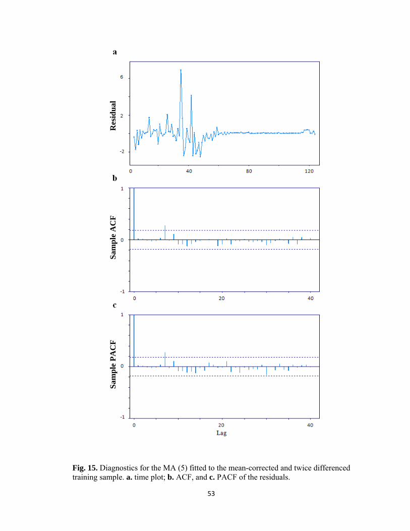
Fig. 15. Diagnostics for the MA (5) fitted to the mean-corrected and twice differenced training sample. a. time plot; b. ACF, and c. PACF of the residuals.

Sam

ple

PA

CF

S

amp

le A

CF

Res

idu

al

 

54  

Fig. 16. Diagnostics for the subset model of MA (5) fitted to the mean-corrected and twice differenced training sample. a. time plot, b. ACF, and c. PACF of the residuals.

Sam

ple

PA

CF

S

amp

le A

CF

R

esid

ual

 

55  

 

Fig. 77. Diagnostics for MA (4) fitted to the mean-corrected and twice differenced training sample. a. time plot, b. ACF, and c. PACF of the residuals.

Sam

ple

PA

CF

S

amp

le A

CF

R

esid

ual

 

56  

Fig. 18. Comparison of the forecasted ERRs using MA (5), subset MA (5) and MA (4) model with the observed data.

 

Table 10 Numerical values of observed ERRs, corresponding observed counts, predicted ERRs (using MA(4)) and corresponding predicted counts for the prediction set

Forecast Horizon

ERRs Counts

Actual Prediction    Actual Prediction 125 4.496 4.493 11 11 126 4.524 4.527 8 9 127 4.567 4.578 10 11 128 4.609 4.611 10 9

4.42

4.47

4.52

4.57

4.62

4.67

ActualMA(5)MA(5) subsetMA(4)

ER

R (

Z3)

1 2 3 4

Forecast horizon

 

57  

6.2 Modeling for ERRR time series

We have six ERRR time series as illustrated in Chapter 4, Fig. 7. In this section, we

will use the R23 series as an example to present the ARIMA and ARFIMA modeling. The

modeling process is similar to that detailed earlier. Fig. 19 shows the ERRR plots with

training sample and prediction set. As in the previous section, we use the last 4 ERRR

values as the prediction set and the remaining as the training sample. Fig. 20 shows the

corresponding time plot, sample ACF and sample PACF, which indicates nonstationary

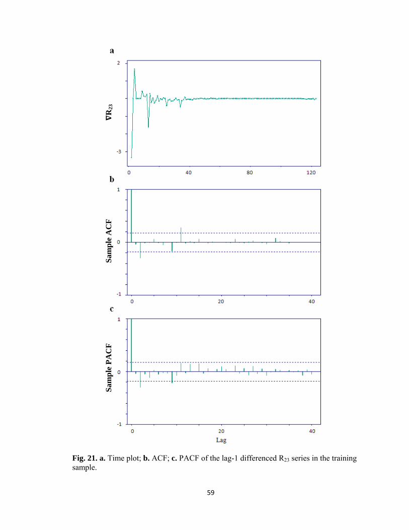
behavior. A difference at lag-1 was taken and Fig. 21 shows the time plot, sample ACF

and sample PACF of the lag-1 differenced series.

Fig. 19. ERRR plots (R23) with training sample and prediction set.

E

RR

R (

R23

)

 

58  

Fig. 20. a. Time plot; b. ACF; c. PACF of R23 in the training sample.

S

amp

le P

AC

F

Sam

ple

AC

F

ER

RR

(R

13)

 

59  

Fig. 21. a. Time plot; b. ACF; c. PACF of the lag-1 differenced R23 series in the training sample.

Sam

ple

PA

CF

S

amp

le A

CF

R

23

 

60  

Next, ARIMA modeling and computational techniques are used to fit the differenced

ERRRs. We set the AR and MA parameters between to be 0 and 5, and after traversing

all possible models, we find the best model is ARMA(4, 2). Fig. 22 is a set of diagnostic

plots produced by ITSM2000 package, which show the ACF and PACF of residuals of

training sample obtained after fitting ARMA (4, 2) model. The AICC statistic is -463.15

and the Ljung-Box test is not significant (p-value = 0.45). The estimated model is given

in the following box:

ARMA(4, 2) Model:

Xt  = - .3176 Xt-1 + .1690 Xt-2 - .1078 Xt-3 + .04347 Xt-4 + Zt + .2380 Zt-1 - .5709 Zt-2   

WN Variance = 0.001159

Looking at the raw data sample ACF in Fig. 20 b, we see that the autocorrelation

decreases very slowly, which indicates a long-term memory. We thus consider using a

fractional differencing parameter, which gives rise to the ARFIMA modeling. We find

that the best such model is ARFIMA (1, 0.498, 1). Fig. 23 is a set of diagnostic plots

produced by ITSM2000 package, which show the ACF and PACF of residuals obtained

from the fitted ARFIMA (1, 0.498, 1) model applied to the training sample. The AICC

statistic is -469.82 and the Ljung-Box test is not significant (p-value = 0.47). The

estimated model is given in the following box.

ARFIMA(1, 0.498, 1) Model:

(1-B) 0.4985 [Xt + .7287 Xt-1] = Zt + 1.0000 Zt-1  

 WN Variance = 0.001056

 

61  

Fig. 22. Diagnostics for ARIMA(4,2) fitted to the mean-corrected and lag-1 differenced training sample. a. time plot, b. ACF, and c. PACF of the residuals.

S

amp

le P

AC

F

Sam

ple

AC

F

R

esid

ual

 

62  

Fig. 23. Diagnostics for ARFIMA(1,0.498,1) fitted to the mean-corrected training sample. a. time plot, b. ACF, and c. PACF of the residuals.

S

amp

le P

AC

F

Sam

ple

AC

F

Res

idu

al

 

63  

 

 

Fig. 24. Comparison of the forecasted ERRRs using ARMA (4, 2) and ARFIMA (1, 0.498, 1) models with the observed values in the prediction set.

We use Fig. 24 to compare the forecasted ERRRs using ARMA (4, 2) and ARFIMA

(1, 0.498, 1) model with the observed values in the prediction set. As defined in the

previous section, we calculated the root mean square error (RMSE) to compare the

accuracy of prediction for these models, and obtained RMSEARMA(4, 2) = 0.008,

RMSEARFIMA(1, 0.498, 1) = 0.003. Hence we choose ARFIMA (1, 0.498, 1) as our final

model and corresponding predicted ERRRs are presented in Table 11.

0.51

0.515

0.52

0.525

0.53

0.535

0.54

Actual

ARMA(4,2)

ARFIMA(1,0.498,1)

1 2 3 4

Forecast horizon

ER

RR

(R

23)

 

64  

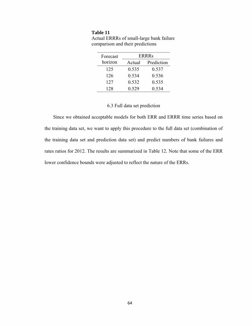
Table 11 Actual ERRRs of small-large bank failure comparison and their predictions

Forecast horizon

ERRRs Actual Prediction

125 0.535 0.537 126 0.534 0.536 127 0.532 0.535 128 0.529 0.534

6.3 Full data set prediction

Since we obtained acceptable models for both ERR and ERRR time series based on

the training data set, we want to apply this procedure to the full data set (combination of

the training data set and prediction data set) and predict numbers of bank failures and

rates ratios for 2012. The results are summarized in Table 12. Note that some of the ERR

lower confidence bounds were adjusted to reflect the nature of the ERRs.

        

 

 

 

 

 

65  

 

 

 

 

 

 

 

 

 

 

 

 

 

 

 

 

 

66  

CHAPTER 7

CONCLUSIONS

The original objective of this study was to examine the relationship between bank

failure status and bank asset size; we wanted to know if they are related or not. We hoped

to use this information to predict the future bank failures. The Pearson’s chi-square test

for contingency tables gave us a positive response. For further study on bank failure and

its prediction based on size, we applied the logistic regression modeling. We obtained the

corresponding prediction rules and results. However, the results were not very

satisfactory.

We then transferred the raw data to ERR and ERRR time series, which provided us

with additional ideas of data analysis. We obtained much valuable information on the

reason for, time period of, and trends of bank failures during the past thirty years. First,

we performed a detailed analysis of the ERR and ERRR time series plots. We separated

1980 to 2011 into three periods: Savings and Loan crisis, the stable period and the Great

Recession crisis. We studied the features of failed bank types during these different

periods. Smaller banks failed more often during the Savings and Loan crisis. However,

banks with larger assets failed more often between 2007:Q1 to 2011:Q4 (Great

Recession).

Additionally, we performed pairwise bank failure rate comparisons using the

conditional test (Przyborowski and Wilenski, 1940). We found that the ERR and ERRR

not only smooth and reduce the volatility of a financial system modeled by a stochastic

process, but also operate as a linking bridge between a classical time series and a point

 

67  

process, which became the most important factor helping us to get our predictions. Based

on the good behaviors of ERR and ERRR time series, a variety of time series modeling

techniques could be applied. We fitted ARIMA and ARFIMA models to the ERR and

ERRR time series and found the resulting predictions of failure counts to be quite

accurate.

 

68  

APPENDIX І

Detailed bank data with bank Status, Periods and Assets (Data file is available upon request, http://fdic.gov/bank/individual/failed/banklist.html)

Bank Status Period Group Assets Log-Assets 1 0 0 1 3015000 14.91911042 1 1 1 3140075.9 14.95975753 0 0 1 3491000 15.0656988

.

.

.

10510 0 0 4 1451969302000.00 28.003941910511 0 0 4 1542984268826.00 28.064739510512 0 0 4 1811678000000.00 28.2252746

Definitions of variables Status: “1” for failed bank and “0” for solvent. Period: “0” for solvent bank, “1” for banks failed between 1980:Q1 and aaaaaaa1995:Q4, “2” for banks failed between 1996:Q1 and 2006:Q4, and aaaaaaa“3” for banks failed between 2007:Q1 and 2011:Q4. Group: “1” for G1, “2” for G2, “3” for G3, and “4” for G4.

 

69  

APPENDIX ІІ

Number of Bank failures during 1980:Q1 to 2011:Q4 by groups.

Quarter Total Small Medium Large Grand 1980Q1 3 3 0 0 0 1980Q2 2 1 1 0 0 1980Q3 2 0 1 1 0 1980Q4 2 2 0 0 0 1981Q1 4 1 3 0 0 1981Q2 1 1 0 0 0 1981Q3 1 1 0 0 0 1981Q4 2 2 0 0 0 1982Q1 4 3 0 0 1 1982Q2 10 8 2 0 0 1982Q3 10 8 1 0 1 1982Q4 8 7 1 0 0 1983Q1 11 6 3 0 2 1983Q2 15 6 4 4 1 1983Q3 10 6 3 0 1 1983Q4 9 6 1 1 1 1984Q1 13 7 4 1 1 1984Q2 30 15 9 4 2 1984Q3 26 15 4 2 5 1984Q4 22 16 3 0 3 1985Q1 28 16 8 4 0 1985Q2 40 21 11 4 4 1985Q3 40 29 4 2 5 1985Q4 46 27 7 2 10 1986Q1 46 20 11 4 11 1986Q2 56 22 13 12 9 1986Q3 57 30 12 7 8 1986Q4 49 22 13 7 7 1987Q1 77 43 13 10 11 1987Q2 64 40 9 9 6 1987Q3 52 28 9 7 8 1987Q4 65 36 13 6 10 1988Q1 65 32 16 12 5 1988Q2 67 37 11 9 10

 

70  

1988Q3 184 47 39 51 47 1988Q4 116 29 28 28 31 1989Q1 72 32 10 12 18 1989Q2 55 28 11 1 15 1989Q3 163 54 41 35 33 1989Q4 99 39 16 15 29 1990Q1 124 38 28 26 32 1990Q2 198 67 48 42 41 1990Q3 109 47 18 23 21 1990Q4 96 27 25 20 24 1991Q1 83 26 11 13 33 1991Q2 77 23 18 14 22 1991Q3 66 21 14 13 18 1991Q4 54 14 10 6 24 1992Q1 51 24 9 5 13 1992Q2 54 12 14 14 14 1992Q3 25 8 6 5 6 1992Q4 55 9 7 10 29 1993Q1 14 5 3 2 4 1993Q2 20 9 3 4 4 1993Q3 19 10 7 1 1 1993Q4 7 2 1 1 3 1994Q1 2 0 0 1 1 1994Q2 6 3 1 1 1 1994Q3 9 1 2 6 0 1994Q4 2 0 1 1 0 1995Q1 3 1 0 1 1 1995Q2 3 1 1 0 1 1995Q3 2 0 1 1 0 1995Q4 1 1 0 0 0 1996Q1 2 1 0 0 1 1996Q2 5 1 2 0 2 1996Q3 3 2 1 0 0 1996Q4 1 0 0 0 1 1997Q1 2 0 0 0 2 1997Q2 1 0 0 0 1 1997Q3 2 0 0 0 2 1997Q4 1 1 0 0 0 1998Q1 0 0 0 0 0 1998Q2 2 1 0 0 1 1998Q3 3 1 0 1 1

 

71  

1998Q4 2 0 0 0 2 1999Q1 1 1 0 0 0 1999Q2 1 1 0 0 0 1999Q3 5 1 2 1 1 1999Q4 3 0 1 1 1 2000Q1 3 1 1 0 1 2000Q2 1 1 0 0 0 2000Q3 2 1 1 0 0 2000Q4 4 0 2 0 2 2001Q1 1 1 0 0 0 2001Q2 3 2 0 0 1 2001Q3 2 1 0 0 1 2001Q4 0 0 0 0 0 2002Q1 6 3 1 0 2 2002Q2 4 1 1 1 1 2002Q3 1 0 1 0 0 2002Q4 2 1 1 0 0 2003Q1 2 0 1 0 1 2003Q2 1 1 0 0 0 2003Q3 0 0 0 0 0 2003Q4 1 1 0 0 0 2004Q1 3 2 1 0 0 2004Q2 1 0 1 0 0 2004Q3 1 1 0 0 0 2004Q4 1 0 0 1 0 2005Q1 0 0 0 0 0 2005Q2 0 0 0 0 0 2005Q3 0 0 0 0 0 2005Q4 0 0 0 0 0 2006Q1 0 0 0 0 0 2006Q2 0 0 0 0 0 2006Q3 0 0 0 0 0 2006Q4 1 0 0 0 1 2007Q1 1 1 0 0 0 2007Q2 0 0 0 0 0 2007Q3 1 0 0 0 1 2007Q4 1 0 1 0 0 2008Q1 3 3 0 0 0 2008Q2 2 1 0 0 1 2008Q3 9 0 1 2 6 2008Q4 12 2 1 2 7

 

72  

2009Q1 21 0 4 8 9 2009Q2 25 1 3 9 12 2009Q3 51 5 11 12 23 2009Q4 46 6 9 12 19 2010Q1 41 7 6 9 19 2010Q2 45 6 9 8 22 2010Q3 41 5 5 15 16 2010Q4 30 3 10 9 8 2011Q1 26 2 7 11 6 2011Q2 22 2 6 8 6 2011Q3 27 3 5 10 9 2011Q4 28 3 5 10 10

 

73  

BIBLIOGRAPHY

Agresti, A., 2002. Categorical Data Analysis, second ed., Wiley, New Jersey.

Akaike, H., 1974. A new look at the statistical model identification. IEEE Trans Aut. Contr. 19, 203-217.

Armstrong, S. J., Collopy, F., 1992. Error measures for generalizing about forecasting methods: empirical comparisons. International Journal of Forecasting 8, 69-80. Box, G.E.P., Jenkins, G.M., 1976. Time Series Analysis: Forecasting and Control. Holden-Day, San Francisco.

Brockwell, P.J., Davis, R.A., 2002. Introduction to Time Series and Forecasting. Second ed., Springer-Verlag, New York.

Cole, R., Wu, Q., 2009. Predicting bank failures using a simple dynamic hazard model, 22nd Australasian Finance and Banking Conference 2009 (AFBC 2009), Sydney 16-18 December.

Cryer, J.D., Chan, K.S., 2008. Time Series Analysis with Applications in R. Second ed., Springer, New York.

Cui, F., 2011. ARIMA models for bank failures: prediction and comparison. UNLV M.S. Thesis. Douglas, C. M., Elizabeth, A.P., Geoffrey, G.V., 2012. Introduction to Linear Regression Analysis. Fifth ed., Wiley, New Jersey.

Freed, N., Glover, F., 1981. A Linear programming approach to the discriminant problem. Decision Sciences 12, 68-74. Glover, F., 1990. Improved linear programming models for discriminant analysis. Decision Sciences 21, 771-785. Halling, M., Hayden, E., 2007. Bank failure prediction: a three-state approach. Working paper, Oesterreichische National Bank and University of Utah. Ho, C.-H., 2008. Empirical recurrent rate time series for volcanism: application to Avachinsky volcano, Russia. Volcanol Geotherm Res 173, 15-25.

Karacabey, A., 2003. Bank failure prediction using modified minimum deviation model. Journal of Risk and Diversification 2, 6-17. Levin, C., Coburn, T., 2011. Wall street and the financial crisis: anatomy of a financial collapse. Majority and Minority Staff Report, April 13.

 

74  

Ljung, G.M., Box, G.E.P., 1978. On a measure of lack of fit in time series models. Biometrika 65, 297-303.

Mankiw, N.G., 2002. Macroeconomics. Fifth ed., Worth, New York.

Mathis, A., 2011. Statistical analysis of fatalities due to vehicle accidents in Las Vegas, NV. UNLV MS Thesis. Przyborowski, J., Wilenski, H., 1940. Homogeneity of results in testing samples from Poisson series, Biometrika 31, 313-323. Shumway, H., Stoffer, S. 2006. Time Series Analysis and Its Applications with R Examples. Springer, New York. Sistrom, L., Garvan, W., 2004. "Proportions, odds, and risk". Radiology 230 (1), 12–9. Smith, R., Sidel, R., 2010. Banks keep failing, no end in sight. Wall Street Journal. September 27.

Sueyoshi, T., 1999. DEA–discriminant analysis in the view of goal programming. European Journal of Operational Research 115, 564–582. Swets, J.A., 1996. Signal detection theory and ROC analysis in psychology and diagnostics: collected papers. Lawrence Erlbaum Associates, Mahwah, NJ.

 

75  

VITA

Graduate College

University of Nevada, Las Vegas

Guancun Zhong

Degree:

Master of Science in Math, 2009

Dalian University of Technology, Dalian

Thesis Title: Analysis of Bank Failure and Size of Assets

Thesis Examination Committee:

Chairperson, Chih-Hsiang Ho, Ph.D.

Committee Member, Amei Amei, Ph.D.

Committee Member, Kaushik Ghosh, Ph.D.

Graduate Faculty Representative, Hualiang Teng, Ph.D.