ANALYSIS OF A HOMEMADE AIR CONDITIONING UNIT

UNIVERSITY OF WATERLOO

GEOFFREY MILBURN 3B CIVIL ENGINEERING

SEPTEMBER 2005

200 University Avenue West Waterloo, ON N2L 3G1 September 19, 2005 Dr. Wei-Chau Xie Associate Chair, Undergraduate Studies Department of Civil Engineering University of Waterloo Waterloo ON N2L 3G1 Dear Sir: This report, entitled “Analysis of a Homemade Air Conditioning Unit” was prepared for the Department of Civil Engineering. This is my third of four required work reports as specified by the Department of Civil Engineering at the University of Waterloo. The purpose of this report is to provide quantifiable analysis of a homemade air conditioning unit which I built during the summer of 2005. The University of Waterloo has long been recognized as one of the most innovative universities in Canada. This past work term, I was fortunate enough to be employed as a WEEF Teaching Assistant under the direction of Dr. Robert McKillop. During this time, I assisted lab sessions, marked assignments, and ensured a smooth transition for first year students into a university environment. This report was prepared entirely by one person and has not received any previous academic credit at this or any other academic institution. I would like to thank Dr. Robert McKillop and my fellow WEEF TAs for their understanding and assistance throughout the term and during my absences for interviews with media outlets. Figures, spreadsheets, and any text completed in partnership with any other person are clearly indicated as such. Sincerely, Geoffrey Milburn ID --------

Analysis of a Homemade Air Conditioning Unit

University of Waterloo

Geoffrey Milburn 3B Civil Engineering

September 2005

ii

Summary

The summer of 2005 was an extremely hot one for Ontario. I was living in a cramped

student house at the time, with no air conditioning. Eventually I ended up constructing a

homemade air conditioner which happened to work quite well, allowing me to get to

sleep easily during one of the hottest summers on record.

This report quantifies the performance and characteristics of the homemade air

conditioner I had constructed. Analysis includes quantification and modeling of the heat

removal capacity and efficiency of the system under varying conditions, and net present

worth analysis of the unit considering all recurring costs. Attention has been paid to the

areas that have received the most frequent questions from those interested in the design.

It was found that the heat removal capacity of the homemade air conditioning system

ranged from approximately 500 BTU/h to 1750 BTU/h as flow rate through the system

ranged from 0.25 L/min to 2.00 L/min. A mathematical model was created to describe the

response of heat removal capacity to changing flow rate.

The efficiency of the system was measured in terms of BTUs removed per litre of water

used. Efficiency varied from approximately 35 BTU/L to 15 BTU/L as flow rate through

the system ranged from 0.25 L/min to 2.00 L/min. Based on the model for variation of

heat removal capacity with flow rate, a model was constructed to describe the variation of

efficiency with flow rate.

Economic analysis of the system was conducted to determine the long term feasibility of

iii

operating the unit. Net present worth calculations were undertaken based on typical usage

patterns at flow rates ranging from 0.25 L/min to 2.00 L/min. It was found that the total

cost of operation (measured by net present worth) varied from approximately $35 to

$130, below the cost of purchasing and operating a commercial air conditioning unit.

It was recommended that the data collected be expanded and refined. Testing at a greater

variety of flow rates and obtaining more results at each flow rate were both suggested. It

was also recommended that more accurate measurement instruments be used. A more

controlled testing location would also improve the consistency and accuracy of results. If

accuracy and number of results are both improved, it may become feasible to further

investigate the mathematical models constructed to describe heat removal capacity and

efficiency.

iv

Table of Contents

Summary ............................................................................................................................. ii

Table of Contents............................................................................................................... iv

List of Tables ...................................................................................................................... v

List of Figures ..................................................................................................................... v

List of Appendices .............................................................................................................. v

1.0 Introduction............................................................................................................. 1

2.0 Description.............................................................................................................. 2

2.1 Materials ............................................................................................................. 2

2.2 Initial Design....................................................................................................... 3

2.3 Final Tested Design ............................................................................................ 3

3.0 Testing..................................................................................................................... 4

3.1 Assumptions........................................................................................................ 4

3.2 General Testing Procedure.................................................................................. 4

4.0 Calculation .............................................................................................................. 5

4.1 Assumptions........................................................................................................ 5

4.2 General Calculation Procedure ........................................................................... 5

5.0 Analysis................................................................................................................... 6

5.1 Energy Analysis .................................................................................................. 6

5.2 Efficiency Analysis............................................................................................. 9

5.3 Economic Analysis ........................................................................................... 11

6.0 Conclusions and Recommendations ..................................................................... 13

6.1 Conclusions....................................................................................................... 13

6.2 Recommendations............................................................................................. 14

References......................................................................................................................... 16

v

List of Tables

Table 1: Calculated Heat Removal Capacity Trendlines.................................................... 7

Table 2: Net Present Worth by Flow Rate ........................................................................ 12

List of Figures

Figure 1: Fan With Attached Copper Coil.......................................................................... 2

Figure 2: Heat Removal Capacity vs Flow Rate Scatterplot .............................................. 7

Figure 3: Heat Removal Capacity vs Flow Rate Trendline ................................................ 8

Figure 4: Heat Removal Efficiency vs Flow Rate Scatterplot............................................ 9

Figure 5: Heat Removal Efficiency vs Flow Rate Trendline............................................ 11

List of Appendices

Appendix A – Excel Calculations..................................................................................... 17

Appendix B – Weather Data for August 3, 2005.............................................................. 23

1

1.0 Introduction

The summer of 2005 was a particularly hot one for Ontario. The mean average

temperature in Toronto for the month of June was a staggering 22.5 ˚C. Environment

Canada meterologist Peter Kimbell was quoted as saying "We've smashed the normal

temperature by almost five degrees. It's a significant record (…) the previous record was

21.7 C in 1949." It was a deadly difference, as three heat related deaths were identified by

Toronto’s coroner’s office during June.

I was living in a cramped student house at the time, with no air conditioning. Nights were

starting to become unbearable, as fans would only stir the hot sticky air around. To top it

off, my house would steadfastly refuse to cool off in the evenings. Eventually I ended up

constructing a homemade air conditioner which happened to work quite well, allowing

me to get to sleep easily during one of the hottest summers on record.

Unexpectedly, I also received significant media attention as a result of a small website I

had put up describing the unit. A quick radio interview with National Public Radio in

Washington led to other radio spots including one with CBC, a front page appearance in

the Kitchener-Waterloo Record, and a segment on CTV’s Canada AM.

This report aims to quantify the performance and characteristics of the homemade air

conditioner I had constructed. Analysis includes quantification and modeling of the heat

removal capacity and efficiency of the system under varying conditions, and net present

worth analysis of the unit considering all recurring costs. Attention has been paid to the

areas that have received the most frequent questions from those interested in the design.

2.0 Description

The unit functioned as a basic heat pump, using water as the transport medium. Cold

water chilled a copper coil, and a fan was then used to push the warm air in the room over

the coil. The warm air heated the coil, removing heat from the air and warming the water

inside the coil. The waste warm water was then removed. A front view of the fan with the

attached copper coil may be seen in Figure 1.

Figure 1: Fan With Attached Copper Coil

2.1 Materials

Materials used included a large oscillating fan, ¼ inch outer diameter (OD) copper

tubing, ¼ inch inner diameter (ID) vinyl tubing, copper wire, a garbage can, garden hose,

pipe insulation, and various small accessories used to attach the components together.

2

3

2.2 Initial Design

The initial design used a basic gravity siphon to force water through the copper coil. A

garbage can, filled with ice water, was placed in an elevated location. Vinyl tubing led

from the garbage can to the copper coil on the back of the fan. The copper coil was

constructed out of approximately 7.5 meters of copper refrigerant tubing, which was

coiled in a spiral on the back of the fan and attached by zipties. Vinyl tubing then led

from the coil to a window. Suction was then applied to the end of the vinyl tubing at the

window to remove any trapped air. Once all air was removed, water flowed freely

through the system due to the siphon effect, and waste warm water was diverted outside.

2.3 Final Tested Design

The initial design possessed several limitations that were later addressed. The first design

limitation was that of the water supply. As built, the system could only cool for the

duration of one garbage pail full of water. In addition, the presence of a large pail of

water in the location to be cooled led to transport difficulties and the risk of flooding. As

such, the design was modified to use a garden hose as the source of cold water. The

garden hose was insulated and then attached to the vinyl tubing previously in the garbage

pail.

The second limitation was that of the cooling performance of the initial copper coil

design. While the coil on the back of the fan led to satisfactory cooling, it was hoped that

moving the coil to the front of the fan and increasing the surface area would lead to

increased performance. To accomplish this, the copper tubing was recoiled on the front of

4

the fan and approximately 30 meters of copper wire was woven in between the coils of

copper tubing. The improvement was immediately noticeable, and verified both

qualitatively and quantitatively.

3.0 Testing

All testing was done over the period of a few hours in the afternoon of August 3, 2005.

The testing location was located outside where the ambient temperature ranged from 29

to 31˚C. Relative humidity ranged from approximately 55 to 60%. The location was

sheltered from wind, but recorded wind speeds ranged between 1.5 and 2.0 m/s.

3.1 Assumptions

It was assumed that the location had a sufficient volume of circulated air such that any

cooling effect generated by the unit would be negligible. This would result in a constant

heat gradient, as opposed to the varying gradient encountered in a closed system. It was

also assumed that any increase in temperature of the water flowing through the system

was due to the performance of the unit. This was deemed to be reasonable, as any

exposed surfaces that would introduce heat to the water were also exposed in typical

operation. The characteristics of the testing location reflected the usual characteristics of

a hot room where the unit would be used. It was also assumed that the temperature of the

water feed was constant.

3.2 General Testing Procedure

Testing was done with the help of an assistant. The temperature of the incoming water

5

supply was measured. Following this, the water supply was modulated to produce a

certain flow rate, which ranged from 0 to 2 L/min in steps of 0.25 L/min. A period of five

minutes was allowed to elapse, to ensure that the unit was at a steady state condition.

Temperature readings were taken at the end of the system, where waste warm water was

released. The amount of water released in thirty seconds was also measured to determine

flow rate more precisely. Finally, a temperature reading of the incoming water source

was taken again to ensure no variation in water feed temperature. If significant variation

was noted in feed temperature, the procedure was repeated. Three readings were taken for

each flow rate.

4.0 Calculation

Calculation of heat removal was based entirely on the measurements taken above, with

no adjustments of any kind. The change in temperature between the inlet and outlet was

known, and combined with the flow rate, a measure of heat removal per unit time could

be found.

4.1 Assumptions

The heat capacity of water was assumed to be 4.19 J/g˚C. The density of water used was

assumed to be 1000 g/L. A joule was assumed to be equivalent to 0.0009485 BTUs.

4.2 General Calculation Procedure

Based on observations recorded previously, inlet and outlet temperatures were known.

This was then used to determine the difference in temperature across the system. The

6

flow rate was also known, which could be used to determine the total change in temperate

for a given volume of water per unit time. The change in temperature for a certain

volume of water could then be converted into an amount of energy. Heat removal was

measured in British Thermal Units per Hour (BTU/h) to coincide with typical metrics of

commercial air conditioners.

5.0 Analysis

Initial analysis involved the calculation of heat removal capacity and the construction of

models for varying flow conditions. Efficiency of the system was also researched, with

removal efficiency measured by BTUs removed per litre of flow. A model of the

efficiency curve was also constructed. Economic assessment of the unit was conducted as

well, including a determination of net present worth of the unit and associated costs for a

typical summer.

5.1 Energy Analysis

Heat removal capacity was calculated for the three readings at each 0.25 L/min interval

between 0.25 L/min and 2 L/min. A scatter plot of heat removal capacity versus flow rate

may be seen in Figure 2.

0

200

400

600

800

1000

1200

1400

1600

1800

2000

0.00 0.50 1.00 1.50 2.00

Flow Rate

Hea

t Rem

oval

Cap

acity

(BTU

/h)

Figure 2: Heat Removal Capacity vs Flow Rate Scatterplot

It can be seen that a clear relationship existed between increasing flow rate and increasing

heat removal capacity. Attempts were made to quantify this relationship by the

application of varying trendlines, including linear, logarithmic, polynomial, power, and

exponential models. The degree of fit was measured by R2, and the model with the

highest R2 value was deemed to be the most accurate model. A summary of the calculated

trendlines may be seen below.

Table 1: Heat Removal Capacity Trendlines

Trendline Model Equation Resulting R2

Value Linear 564.82 515.67y x= + 0.7552

Logarithmic 494.45ln 1181.5y x= + 0.7642 Polynomial 2124.29 844.59 399.25y x x= − + + 0.7643

Power 0.50431117.1y x= 0.8253 Exponential 0.5461585.85 xy e= 0.7329

7

It can be seen that the power model produced the most accurate trendline. With additional

investigation, this trendline model was refined to reflect characteristics of the system. It

was noted that the exponent 0.5043 was quite close to 0.5, or the square root of x.

Additionally, the coefficient of 1117.1 was quite similar to the average heat removal

capacity at a unit flow rate, 1022.2 BTU/h. This custom trendline ( y 1022.2 x= )was

then analyzed for degree of fit, and was found to have an R2 value of 0.7943. A

scatterplot of values with the custom trendline may be seen below.

0

200

400

600

800

1000

1200

1400

1600

1800

2000

0.00 0.50 1.00 1.50 2.00

Flow Rate (L/min)

Hea

t Rem

oval

(BTU

/h)

Figure 3: Heat Removal Capacity vs Flow Rate Trendline

It is suspected that for systems of this type, the following equation may be used to

describe the variation of heat removal with flow rate.

1H uH f= (1)

In this case, H represents heat removal, H1 the heat removal at a unit flow rate, f the flow

8

rate, and u a constant which adjusts for units. The constant u had the value of 1 (min/L)0.5

in this case, and 1 (time/volume)0.5 in the general case. It is suspected that u may vary

from unity depending on the friction characteristics of the tubing, characteristics of the

unit, and the external environment, but insufficient data is present to quantify this to any

degree of accuracy. Unfortunately, this model does not lend itself to optimization easily,

as there are no local maxima within a practical flow rate range (defined as 0 to 2 L/min).

5.2 Efficiency Analysis

Heat removal efficiency was calculated for the three readings at each 0.25 L/min interval

between 0.25 L/min and 2 L/min. Efficiency was determined by BTUs removed per litre

of water used. A scatter plot of heat removal efficiency versus flow rate may be seen in

Figure 4 below.

0

5

10

15

20

25

30

35

40

0.0 0.5 1.0 1.5 2.0

Flow Rate

Hea

t Rem

oval

Effi

cien

cy (B

TU/L

)

Figure 4: Heat Removal Efficiency vs Flow Rate Scatterplot

9

It can be seen that there exists a clear relationship between increasing flow rate and

decreasing heat removal efficiency. Modeling this relationship may be accomplished by

assuming the model for variation of heat removal 1H uH f= is valid. Efficiency may

then be modeled with the following equation.

1

1

uH fHEf f

uEEf

= =

⇒ =

(2)

For the above, E represents heat removal efficiency, E1 the heat removal efficiency at a

unit flow rate, f the flow through the system, and u a constant adjusting for units identical

to that in the heat removal capacity model. The equation was derived from the fact that

efficiency in this case is simply defined as heat removal divided by flow rate.

For the system analysed, E1 is equal to H1 divided by 60 minutes per hour (17.036

BTU/min). This is necessary to produce results in terms of BTU/L, as heat removal

capacity was expressed in BTU/h and flow rate in L/min. The efficiency trendline can

therefore be defined as 0.517.036y x−= , resulting in a R2 value of 0.8510. This may be

seen in Figure 5 on the next page.

10

0

5

10

15

20

25

30

35

40

0.0 0.5 1.0 1.5 2.0

Flow Rate (L/min)

Hea

t Rem

oval

Effi

cien

cy (B

TU/L

)

Figure 5: Heat Removal Efficiency vs Flow Rate Trendline

It can be seen that this model fits quite well with the data in both a quantitative and

qualitative sense. Unfortunately, this model also does not lend itself to optimization

easily, as there are no local maxima within a practical flow rate range (defined as 0 to 2

L/min).

5.3 Economic Analysis

While the initial cost of the unit was quite reasonable at approximately twenty-five

dollars, this means little if the recurring costs to run the unit are excessive. To determine

the economic feasibility of running the system on a frequent basis, net present worth

analysis was undertaken.

Net present worth calculations were undertaken for flow rates between 0 and 2 L/min, in

0.25 L/min increments. It was assumed that flow rate was constant, the initial cost of the

11

12

unit was 25$, the cost of one cubic meter of water including sewage charges was $1.68,

and that the unit was run for 4 days a week, 8 hours a day, for the four months of

summer. A discount rate of 2.5% per annum was used, the rate of return available in the

summer 2005 period on a liquid cash savings account. Calculation results may be seen

below.

Table 2: Net Present Worth by Flow Rate

Flow Rate (L/min)

Net Present Worth

0.25 $37.85 0.50 $50.70 0.75 $63.55 1.00 $76.40 1.25 $89.25 1.50 $102.10 1.75 $114.95 2.00 $127.80

The values calculated were all found to be well within the budgetary range of a typical

university student. More importantly, they were far below the cost of purchasing and

running a commercial air conditioning unit. The cheapest available unit at the time of

construction was found to be $129.99. Even without considering the significant cost of

electricity to run the unit, this was above the net present worth of building and running

the homemade system for four months. It would make little sense to spend more on a

homemade unit when a ready made alternative was available for cheaper, excluding

intangible factors such as the pleasure of building.

6.0 Conclusions and Recommendations

6.1 Conclusions

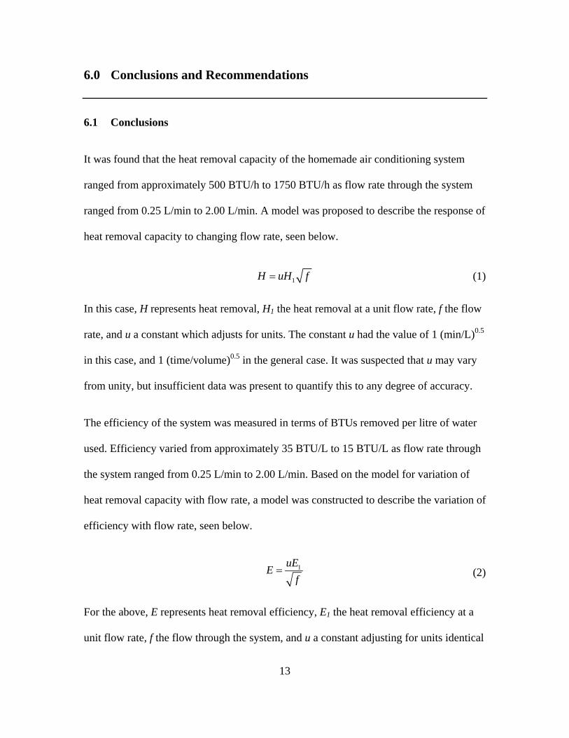
It was found that the heat removal capacity of the homemade air conditioning system

ranged from approximately 500 BTU/h to 1750 BTU/h as flow rate through the system

ranged from 0.25 L/min to 2.00 L/min. A model was proposed to describe the response of

heat removal capacity to changing flow rate, seen below.

1H uH f= (1)

In this case, H represents heat removal, H1 the heat removal at a unit flow rate, f the flow

rate, and u a constant which adjusts for units. The constant u had the value of 1 (min/L)0.5

in this case, and 1 (time/volume)0.5 in the general case. It was suspected that u may vary

from unity, but insufficient data was present to quantify this to any degree of accuracy.

The efficiency of the system was measured in terms of BTUs removed per litre of water

used. Efficiency varied from approximately 35 BTU/L to 15 BTU/L as flow rate through

the system ranged from 0.25 L/min to 2.00 L/min. Based on the model for variation of

heat removal capacity with flow rate, a model was constructed to describe the variation of

efficiency with flow rate, seen below.

1uEEf

= (2)

For the above, E represents heat removal efficiency, E1 the heat removal efficiency at a

unit flow rate, f the flow through the system, and u a constant adjusting for units identical

13

14

to that described above. The equation was derived from the fact that efficiency in this

case is simply defined as heat removal capacity divided by flow rate.

Economic analysis of the system was conducted to determine the long term feasibility of

operating the unit. Net present worth calculations were undertaken based on typical usage

patterns at flow rates ranging from 0.25 L/min to 2.00 L/min. It was found that the total

cost of operation (measured by net present worth) varied from approximately $35 to

$130, below the cost of purchasing and operating a commercial air conditioning unit.

6.2 Recommendations

Increasing the number of data points available would greatly clarify the conclusions of

this report, particularly the mathematical models describing heat removal capacity and

efficiency. Testing at a greater variety of flow rates and obtaining more results at each

flow rate are both suggested.

Accuracy of the measurements could stand to be improved greatly. The principal

limitation was that of measuring temperature. The thermometer used for obtaining the

data in this report was only able to report results in steps of one degree. This led to

inaccuracy as the range of temperature values found was quite small, which caused

significant “jumps” in results if temperature readings varied as little as one degree. It is

recommended that more accurate measurement instruments be used.

A more controlled testing location would also improve the consistency and accuracy of

results. Variation in feed water temperature, ambient temperature, humidity, and wind

speed could have all affected results. An ideal location would be a testing chamber where

15

environmental conditions could be kept constant

If accuracy and number of results are both improved, it may become feasible to

investigate the characteristics of the constant u further. It is suspected that the constant u

is related to the degree of internal friction in the tubing and other factors, however,

further investigation is required to determine if in fact this constant varies from unity.

16

References

CBC News Online. INDEPTH : Summer Sense – Heat Waves.

http://www.cbc.ca/news/background/summersense/. August 2005.

Milburn, Geoffrey. Homebrew AC. http://www.eng.uwaterloo.ca/~gmilburn/ac/. August

2005.

17

Appendix A – Excel Calculations

23

Appendix B – Weather Data for August 3, 2005