ANALYSIS OF 3D AND 4D PROTON TREATMENT PLANNINGFOR HEPATIC TUMORS

ARCHIVESBy

Agata El: bieta Wi~niowska

SUBMITTED TO THE DEPARTMENT OF NUCLEAR SCIENCEAND ENGINEERING

IN PARTIAL FULFILLMENT OF THE REQUIREMENTS FOR THE DEGREE OF

BACHELOR OF SCIENCE IN NUCLEAR SCIENCE AND ENGINEERINGAT THE

MASSACHUSETTS INSTITUTE OF TECHNOLOGY

JUNE 2011

Agata Wisniowska. All Rights Reserved.

The author hereby grants to MIT permission to reproduce and to distribute publiclyPaper and electronic copies of this thesis document in whole or in part.

Signature of Author:--

Agata Wisniowska

Department of Nuclear Science and Engineering

May 191h 2011Al

Certified by:

Certified by:

Richard Lanza

Senior Research Scientist, Department of Nuclear Science and Engineering

/) Thesis Supervisor

George T.Y. Chen

..,- Professor of Radiation Oncology, Harvard Medical School

Thesis Reader

Accepted by:p

Dennis Whyte

Professor of Nuclear Science and Engineering

Chairman, NSE Committee for Undergraduate Students

ANALYSIS OF 3D AND 4D PROTON TREATMENT PLANNINGFOR HEPATIC TUMORS

By

Agata Elzbieta Wisniowska

Submitted to the Department of Nuclear Science and Engineering on May 19 th 2011In partial Fulfillment of the Requirements for the Degree of

Bachelor of Science in Nuclear Science and Engineering

ABSTRACTThe purpose of this study is to assess the difference between 4D liver dose calculations versusstandard 3D treatment planning and to investigate the dosimetric gain of gating on radiation dose tonormal tissue. 4DCT scans are collected for 25 patients with hepatic tumors treated by protonradiotherapy. The 4D treatment planning process explicitly takes into account respiratory motion ofabdominal organs. A 4DCT scan consists of 10 3D anatomical states, each at an instant of time in therespiratory cycle. 4D treatment planning includes 1) propagating the target contours, drawn by aphysician on one phase, to all breathing phases using deformable registration, 2) calculating thecompensating bolus for proton therapy, and then 3) calculating 4D dose distributions. Dose volumehistograms are used to compute the effective uniform dose (EUD) delivered to normal liver.

We found that 4DCT planning always results in a larger EUD to normal liver when compared withdose from a 3DCT plan. The mean EUD difference between 4D and 3D planning is 3.8Gy(o= 1.9Gy, p<0.000 1). Gated 4D treatment planning results in a lower EUD to normal liver comparedto ungated planning, with a mean difference of 2.9 Gy (a=1.9Gy, p<0.0001). The EUD difference isonly weakly correlated with the magnitude of the superior-inferior (S-I) tumor motion (r=0.59 for

4D/3D, r=0.48 for ungated/gated). The AEUD correlation with clinical target volume (CTV) (asfraction of liver volume) is much weaker (r-0.31 for 4D/3D, r=0.26 for ungated/gated). There wasno evidence that the tumor position within the liver influenced the AEUD. This study suggests thatphysicians should consider 4D treatment planning if the risk of normal tissue complications is high.Normal tissues may also be significantly spared by gated treatment as a motion managementstrategy.

Thesis Supervisor: Richard Lanza

Title: Senior Research Scientist

2

INTRODUCTION

Radiation treatment for malignancies has been used for over 100 years since the discovery of X-rays

in 1895 by Wilhelm Roentgen. Radiation therapy refers to the medical use of ionizing radiation to

treat malignant tumors in patients. As radiation transits tissue, it deposits energy in both normal and

diseased tissues, resulting in biological effects. The desired effect is killing tumor cells; an undesired

side-effect is damage to normal tissues.

Accurate calculation of the dose delivered to normal tissue is crucial for effective radiation therapy:

underestimating normal tissue exposure can lead to treating patients with doses higher than is safe,

which could lead to radiation-associated injury to the liver (13), while overestimating healthy tissue

irradiation can overconstrain how much radiation can be delivered to the tumor and lower tumor

control probability. Accuracy of dosimetry to normal tissue is especially important for dose

escalation studies, which often prescribe doses near the maximum dose tolerated by normal tissue in

such studies as (14).

In addition to random setup variations during fractionated treatment (15), respiratory motion poses a

challenge for effective treatment. This problem can be addressed by organ motion reduction

strategies. In principle, tumor irradiation could be delivered at breath-hold to minimize tumor

movement (16): this method has been reported to be better than irradiation during free respiration

(17). Breath hold during treatment, however, has its limitations because the breath hold

reproducibility is an issue: it is difficult for the patients to consistently hold their breath for the

duration of the treatment. Moreover, this varies from patient to patient, introducing a large

uncertainty in tumor position for treatment planning.

3

While some groups argue that tumor motion has negligible effect on photon treatment planning

(dose volume histograms (DVHs)) (e.g., 18), others consider liver motion an important issue and

include it in their calculations (19). Conventional 3D treatment planning based on a single CT scan,

does not explicitly consider tumor motion during treatment. Rosu et al. (20) modeled both geometric

uncertainties in photon treatment and ID (superior-inferior) tumor motion to account for breathing,

and found that 3DCT-based treatment planning both underestimated and overestimated the dose to

normal tissue as compared to their 4D planning model. Their model used mathematical convolution

of a static dose distribution with a motion kernel as an approximation of 4D movement instead of the

actual 4D calculation for each breathing phase. Additionally, Rosu's group assumed rigid structure

contours instead of propagating the contours drawn for one breathing phase to all other phases using

deformable registration.

In this study, we examine the question of how 4D treatment planning (TP) differs in estimating the

dose to normal tissues from 3DTP. 4DCT scans are used in 4DTP to quantify tumor and normal

tissue motion. Unlike Rosu, we are interested in calculating the impact of motion on proton beam

radiotherapy. This study is clinically relevant because patients are being treated with protons at

MGH. The advantage of proton therapy in treatment of hepatic tumors is that it has been reported to

reduce the normal liver irradiated as compared to photons (21).

4DCT data comprise separate CT scans taken over the course of the breathing cycle (ten scans

equally spaced in breathing cycle phases TOO-T90), and allow accurate determination of the dose

delivered to the tumor and surrounding tissue as the organ of interest moves with the patient's

breathing. In contrast with the limited ID movement considered in previous studies (20), we use the

4

4D treatment planning software Aqualyzer (22) to account for full three-dimensional effects of

breathing (i.e., superior-inferior, anterior-posterior, and right-left organ movement), and use

Plastimatch deformable registration (24) to propagate tumor contours from the phase in which they

were drawn to all other breathing phases based on tissue density differences. While a similar tool

exists (32) that takes 3D sets of data at different respiratory phases, propagates the contours, and

performs the calculation on each data set, Aqualyzer had many additional features that facilitated

data analysis, such as customized structures, movies of organ motion during breathing, and summary

of structure motion.

BACKGROUND

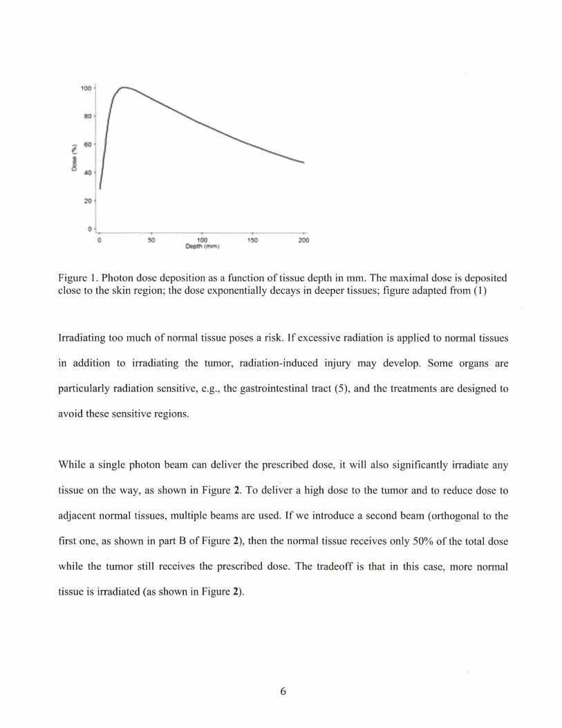
The earliest treatments used photon beams to irradiate tumors. Photon energy deposition to tissue

peaks close to the skin and then decays in an exponential manner (see Figure 1). Thus skin and

tissues close to the skin receive the highest dose even though most frequently the actual tumor lies

much deeper in the body. Because of exponential attenuation, the beam continues irradiating tissues

past the tumor.

5

10C),

I 60*

20 '

0~

0I ' 100

Oe I f-ISO

Figure 1. Photon dose deposition as a function of tissue depth in mm. The maximal dose is depositedclose to the skin region; the dose exponentially decays in deeper tissues; figure adapted from (1)

Irradiating too much of normal

in addition to irradiating the

particularly radiation sensitive,

avoid these sensitive regions.

tissue poses a risk. If excessive radiation is applied to normal tissues

tumor, radiation-induced injury may develop. Some organs are

e.g., the gastrointestinal tract (5), and the treatments are designed to

While a single photon beam can deliver the prescribed dose, it will also significantly irradiate any

tissue on the way, as shown in Figure 2. To deliver a high dose to the tumor and to reduce dose to

adjacent normal tissues, multiple beams are used. If we introduce a second beam (orthogonal to the

first one, as shown in part B of Figure 2), then the normal tissue receives only 50% of the total dose

while the tumor still receives the prescribed dose. The tradeoff is that in this case, more normal

tissue is irradiated (as shown in Figure 2).

6

A1 B

100%

100%

Figure 2. Photon dose deposition in the body. A: One beam delivers 100% of the dose to both thetumor (in green) and to normal tissue (white regions). B: Two orthogonal beams each carrying 50%of the dose: as a result the normal tissue receives 50% of the dose while the tumor still receives100% of the dose; figure adapted from (6)

Conformal radiotherapy, with uniformly illuminated fields being convergent, generally only results

in convex high dose regions (as in Figure 2). Uniform beams cannot be easily used to form concave

dose distributions, where there is a cold region (e.g. spinal cord) within a U shaped target (e.g. tumor

that is U shaped and has a critical dose limiting structure within the U). In the 1990's, a more

advanced delivery method was developed to produce concave distributions, named intensity-

modulated radiation therapy (IMRT), which typically uses 5-7 intensity modulated photon beams

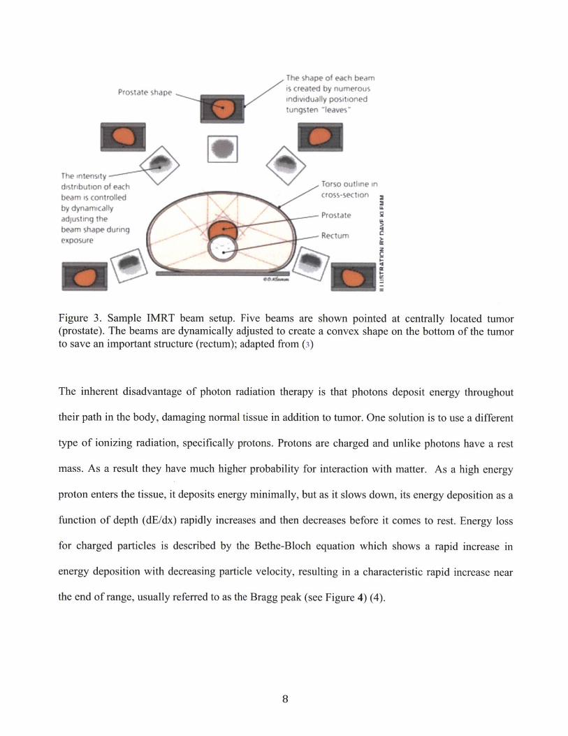
(2). Figure 3 shows the principle of IMRT. Here, there are 5 beams in the example, each entering

from a different angle. Each beam covers the tumor width, but has a non-uniform (i.e., intensity

modulated) beam profile. The cumulative dose from all five fields delivers the prescribed dose to the

tumor, but also can spare a critical structure adjacent to the target (rectum in the example below).

7

Prostate shape

The shape of each bPamis created by numerousinidividuavy positioed

The ritensyyd str thution of eachbeam is ontrolledby dynamcaPyadjusting thebeam shape duringexposure (00

Torso outhine incross-sectio ri

Prostate

Rectum

Figure 3. Sample IMRT beam setup. Five beams are shown pointed at centrally located tumor(prostate). The beams are dynamically adjusted to create a convex shape on the bottom of the tumorto save an important structure (rectum); adapted from (3)

The inherent disadvantage of photon radiation therapy is that photons deposit energy throughout

their path in the body, damaging normal tissue in addition to tumor. One solution is to use a different

type of ionizing radiation, specifically protons. Protons are charged and unlike photons have a rest

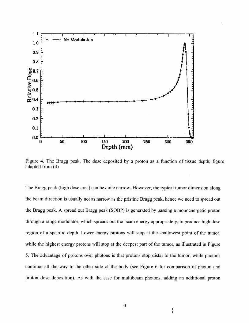
mass. As a result they have much higher probability for interaction with matter. As a high energy

proton enters the tissue, it deposits energy minimally, but as it slows down, its energy deposition as a

function of depth (dE/dx) rapidly increases and then decreases before it comes to rest. Energy loss

for charged particles is described by the Bethe-Bloch equation which shows a rapid increase in

energy deposition with decreasing particle velocity, resulting in a characteristic rapid increase near

the end of range, usually referred to as the Bragg peak (see Figure 4) (4).

8

I I -- -, --No Modulaion

09

~0.8

090.7

90.4

0.3

0,2

0.1

0 50 100 150 200 250 300 350Depth (mm)

Figure 4. The Bragg peak. The dose deposited by a proton as a function of tissue depth; figureadapted from (4)

The Bragg peak (high dose area) can be quite narrow. However, the typical tumor dimension along

the beam direction is usually not as narrow as the pristine Bragg peak, hence we need to spread out

the Bragg peak. A spread out Bragg peak (SOBP) is generated by passing a monoenergetic proton

through a range modulator, which spreads out the beam energy appropriately, to produce high dose

region of a specific depth. Lower energy protons will stop at the shallowest point of the tumor,

while the highest energy protons will stop at the deepest part of the tumor, as illustrated in Figure

5. The advantage of protons over photons is that protons stop distal to the tumor, while photons

continue all the way to the other side of the body (see Figure 6 for comparison of photon and

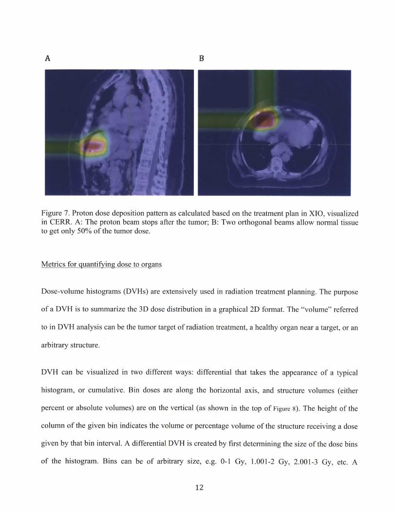
proton dose deposition). As with the case for multibeam photons, adding an additional proton

9

beam decreases the dose to the normal tissue as shown in Figure 7. Unlike photons, though,

protons stop after the tumor and hence spare more normal tissue.

1,l

1.0

0.9

0.8

WO.

0-4

0.3

0.2

0.1

0.00 50 150 200

Depth (mm)250

Figure 5. Spread out of the Bragg peak as a result of adding modulation to the original proton beam.As the beam is more modulated (more spread out in energy), protons travel to different depths andcover the entire tumor depth. Protons with lower energy stop closer to the skin and protons withhigher energy travel deeper. The spread out in energy is represented as the spread out in wavelengthof protons in the figure (figure adapted from 4)

10

photonsp /oton

peaknP

1 .0

0.8 -

0.4-

0.2 -

0.00 10 20

DEPTH (em)

ragg

30 4

Figure 6. Comparison of spread out Bragg peak (SOBP) to photon dose deposition pattern. The Keydifference is that protons stop distal to the tumor while photons continue to deposit energy.Additionally, protons have the advantage in the proximity to the skin over photons because protonsdeposit lower energy as they enter the body and their energy deposition increases towards the Braggpeak. Photons, on the other hand, deposit larger amount of energy to the region close to the skin thanto the actual tumor. As a result photons deposit more energy to the normal tissue close to the skinthan protons do; figure adapted from (7)

11

4 ~

-~4. 4.

U)0

A

B

Figure 7. Proton dose deposition pattern as calculated based on the treatment plan in XIO, visualizedin CERR. A: The proton beam stops after the tumor; B: Two orthogonal beams allow normal tissueto get only 50% of the tumor dose.

Metrics for quantifying dose to organs

Dose-volume histograms (DVHs) are extensively used in radiation treatment planning. The purpose

of a DVH is to summarize the 3D dose distribution in a graphical 2D format. The "volume" referred

to in DVH analysis can be the tumor target of radiation treatment, a healthy organ near a target, or an

arbitrary structure.

DVH can be visualized in two different ways: differential that takes the appearance of a typical

histogram, or cumulative. Bin doses are along the horizontal axis, and structure volumes (either

percent or absolute volumes) are on the vertical (as shown in the top of Figure 8). The height of the

column of the given bin indicates the volume or percentage volume of the structure receiving a dose

given by that bin interval. A differential DVH is created by first determining the size of the dose bins

of the histogram. Bins can be of arbitrary size, e.g. 0-1 Gy, 1.001-2 Gy, 2.001-3 Gy, etc. A

12

B

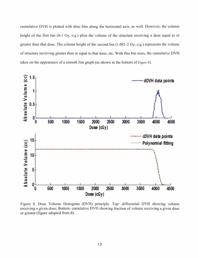
cumulative DVH is plotted with dose bins along the horizontal axis, as well. However, the column

height of the first bin (0-1 Gy, e.g.) plots the volume of the structure receiving a dose equal to or

greater than that dose. The column height of the second bin (1.001-2 Gy, e.g.) represents the volume

of structure receiving greater than or equal to that dose, etc. With fine bin sizes, the cumulative DVH

takes on the appearance of a smooth line graph (as shown in the bottom of Figure 8).

45 %

E

0.6

9 0S0

UU

5=0

0

=00

4*

15

10

5

0L

dDVH data points

500 1000 1500 2000 2500Du(dy)

3000 350 4000 4600

--wq cDVH dab pointsPolynoniA Iting

0 500 1000 1500 2000 200 3M 350 4000 4600Dow (dy)

Figure 8. Dose Volume Histogram (DVH) principle. Top: differential DVH showing volumereceiving a given dose; Bottom: cumulative DVH showing fraction of volume receiving a given doseor greater (figure adopted from 8).

13

Lyman's normal tissue complication probability (NTCP) (27) is a common means of comparing the

relative goodness of rival treatment plans. The plan that produces the same tumor control probability

(same dose to tumor) while sparing normal tissues (plan with lower NTCP) identifies the better plan.

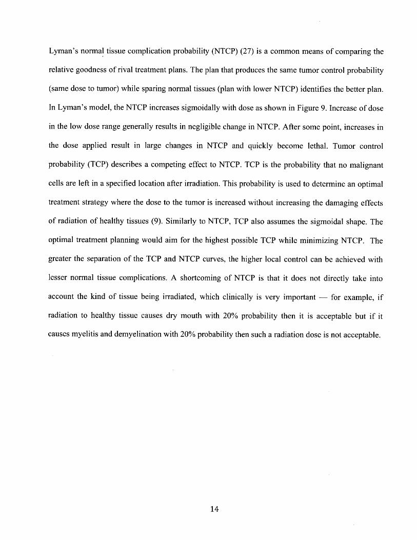
In Lyman's model, the NTCP increases sigmoidally with dose as shown in Figure 9. Increase of dose

in the low dose range generally results in negligible change in NTCP. After some point, increases in

the dose applied result in large changes in NTCP and quickly become lethal. Tumor control

probability (TCP) describes a competing effect to NTCP. TCP is the probability that no malignant

cells are left in a specified location after irradiation. This probability is used to determine an optimal

treatment strategy where the dose to the tumor is increased without increasing the damaging effects

of radiation of healthy tissues (9). Similarly to NTCP, TCP also assumes the sigmoidal shape. The

optimal treatment planning would aim for the highest possible TCP while minimizing NTCP. The

greater the separation of the TCP and NTCP curves, the higher local control can be achieved with

lesser normal tissue complications. A shortcoming of NTCP is that it does not directly take into

account the kind of tissue being irradiated, which clinically is very important - for example, if

radiation to healthy tissue causes dry mouth with 20% probability then it is acceptable but if it

causes myelitis and demyelination with 20% probability then such a radiation dose is not acceptable.

14

OOOO- mo -O-M

Increasing

,p, ~'

/

IIII umor Increasing

cell kill likelihood ofside effect

0)

Tumor - TumorW-O- - Normal

DoseFigure 9. A schematic of NTCP as a function of dose. The effects on the y-axis correspond to thelikelihood of complication (NTCP) (dashed line) and the probability of tumor control (solid line). Asthe dose increases, the effect increases. The optimal treatment is determined by maximizing TCP andsimultaneously minimizing NTCP; figure adapted from (11)

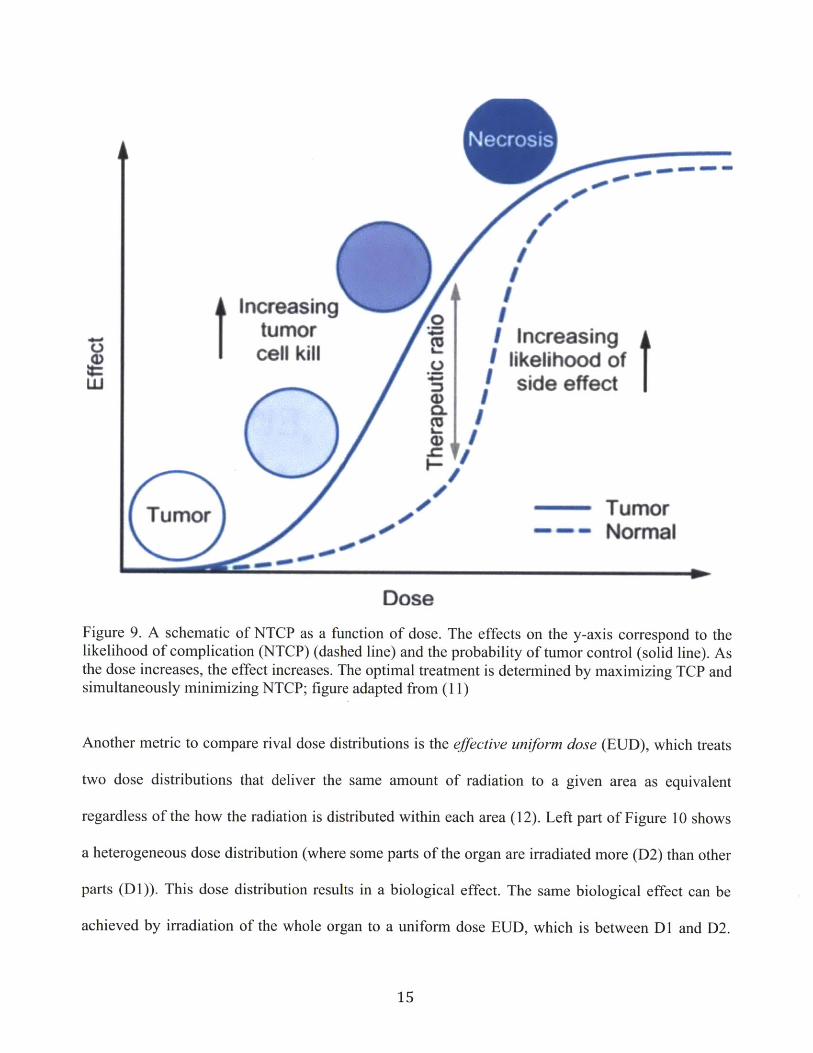
Another metric to compare rival dose distributions is the effective uniform dose (EUD), which treats

two dose distributions that deliver the same amount of radiation to a given area as equivalent

regardless of the how the radiation is distributed within each area (12). Left part of Figure 10 shows

a heterogeneous dose distribution (where some parts of the organ are irradiated more (D2) than other

parts (Dl)). This dose distribution results in a biological effect. The same biological effect can be

achieved by irradiation of the whole organ to a uniform dose EUD, which is between Dl and D2.

15

E ecrostsEl

The principle behind EUD is hence explained: the uneven dose distribution on the left is represented

by the equivalent dose uniformly distributed over the same area as shown on the right. Unlike

NTCP, which models the actual clinical complication probability and is calibrated by case studies,

EUD is always well defined, and therefore makes a good comparison metric.

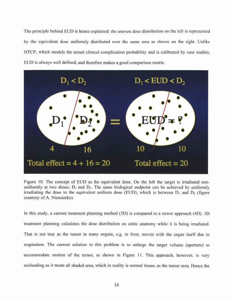
Figure 10. The concept of EUD as the equivalent dose. On the left the target is irradiated non-uniformly at two doses: D1 and D2. The same biological endpoint can be achieved by uniformlyirradiating the dose to the equivalent uniform dose (EUD), which is between D, and D2 (figurecourtesy of A. Niemierko).

In this study, a current treatment planning method (3D) is compared to a newer approach (4D). 3D

treatment planning calculates the dose distribution on static anatomy while it is being irradiated.

That is not true as the tumor in many organs, e.g. in liver, moves with the organ itself due to

respiration. The current solution to this problem is to enlarge the target volume (aperture) to

accommodate motion of the tumor, as shown in Figure 11. This approach, however, is very

misleading as it treats all shaded area, which in reality is normal tissue, as the tumor area. Hence the

16

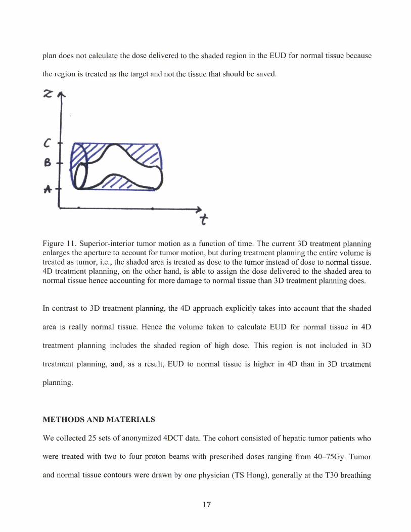
plan does not calculate the dose delivered to the shaded region in the EUD for normal tissue because

the region is treated as the target and not the tissue that should be saved.

tFigure 11. Superior-interior tumor motion as a function of time. The current 3D treatment planningenlarges the aperture to account for tumor motion, but during treatment planning the entire volume istreated as tumor, i.e., the shaded area is treated as dose to the tumor instead of dose to normal tissue.4D treatment planning, on the other hand, is able to assign the dose delivered to the shaded area tonormal tissue hence accounting for more damage to normal tissue than 3D treatment planning does.

In contrast to 3D treatment planning, the 4D approach explicitly takes into account that the shaded

area is really normal tissue. Hence the volume taken to calculate EUD for normal tissue in 4D

treatment planning includes the shaded region of high dose. This region is not included in 3D

treatment planning, and, as a result, EUD to normal tissue is higher in 4D than in 3D treatment

planning.

METHODS AND MATERIALS

We collected 25 sets of anonymized 4DCT data. The cohort consisted of hepatic tumor patients who

were treated with two to four proton beams with prescribed doses ranging from 40-75Gy. Tumor

and normal tissue contours were drawn by one physician (TS Hong), generally at the T30 breathing

17

phase. The treatment beam parameters used in 4D calculations were those used to actually treat the

patient (same field directions, beam weights, field margins, etc.).

Subsequently, we loaded the 4DCT data from all 10 breathing phases (TOO-T90) with the

corresponding contours of the targets and the important structures (liver, kidney, stomach, etc.)

together with the corresponding beam parameters, which include beam angles and weight, prescribed

dose, distal margin, and the smearing radius, used in treatment into Aqualyzer (22) (the details of

how Aqualyzer works are included in Appendix A), a research treatment planning system that uses

the pencil-beam algorithm (23) to calculate the dose in 4D. Aqualyzer then calculates the

compensating bolus based on all breathing phases. To generate 3D planning dose distributions, we

replicated the data from phase T30 for all breathing phases and used the same dose calculation

algorithm as for 4D. The volume-of-interest (VOI) contours were propagated- to all the other

breathing phases within Aqualyzer using Plastimatch deformable registration (24). Aqualyzer then

calculated and returned the 4D dose distribution and the dose volume histograms (DVHs) for each

patient for each of the structures (organs) for which the contours were provided.

The target for 4D treatment planning was defined by taking the target from the treatment plan

performed by the commercial treatment planning program XIO (25) and applying the smear

according to the prescription. Aqualyzer ensured that the target was fully covered in all breathing

phases. For the 3D treatment planning calculation, the target was also defined as the target from the

XIO plan, but it was whatever this target was at phase T30. Hence it did not account for the target

movement. The smearing was applied as prescribed (an in depth description of Aqualyzer

calculation details is attached in Appendix A).

18

Using the DVH for the accumulated dose (i.e., the dose summed over all the breathing phases) for

both gated (T40-T60) and ungated scenarios, we computed the effective uniform dose (EUD) (12)

as described in (27,26) based on a normalized dose of 60Gy (regardless of the actual dose

prescribed) delivered in a 15-fraction schedule and corrected to 1.5Gy/fraction for all cases to avoid

differences in EUD due to dose differences (with the parameters as follows: r=2, RBEmae=1, Lyman

n=0.97). A sample spreadsheet of this calculation is attached in Appendix B.

To determine if the mean difference in EUD between 3D and 4D treatment planning, and between

gated and ungated treatment, statistically differs from zero we performed one-sample t-tests. We

used Pearson's correlation coefficient to evaluate the correlation between the mean difference in

EUD and tumor size, as well as superior-inferior (S-I) motion.

RESULTS

Benchmarking 4D Treatment Planning

In order to validate Aqualyzer as a tool to plan treatment, we compared the 3D Aqualyzer treatment

plans to those generated by XIO (28), a commercially established treatment planning program (see

Table 1 for comparison between XIO and Aqualyzer). To compare the computed doses for each

treatment plan, we used CERR (29) to create a dose subtraction image from the distributions

computed by Aqualyzer and XIO, and visually evaluated the differences. A representative case is

shown in Figure 12. Since the dose distributions are similar in all 3 views (coronal, sagittal and

transverse), we concluded that Aqualyzer was sufficiently accurate and reliable and proceeded with

the study.

19

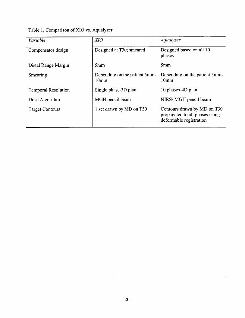
Table 1. Comparison of XIO vs.

Variable XIO Aqualyzer

Compensator design Designed at T30; smeared Designed based on all 10phases

Distal Range Margin 5mm 5mm

Smearing Depending on the patient 5mm- Depending on the patient 5mm-10mm 10mm

Temporal Resolution Single phase-3D plan 10 phases-4D plan

Dose Algorithm MGH pencil beam NIRS/ MGH pencil beam

Target Contours 1 set drawn by MD on T30 Contours drawn by MD on T30propagated to all phases usingdeformable registration

20

Aqualyzer.

a.

bj

C.

Figure 12. 3D Aqualyzer and 3D XIO plans' CERR subtraction images. (a) coronal view, (b) sagittalview, and (c) transverse view. The colorwash scale on the left is in units of Gy. The differences (inthe rightmost column) are very small, which indicates that Aqualyzer dose distribution is similar toXIO plan. The yellow high dose areas outside of the body (in the rightmost column) result from XIOplan ending closer to patient's body than Aqualyzer plan.

4DCT Quality

In selecting cases for analysis we took into account the quality of the 4DCT scans. For each patient,

we examined all 10 breathing phases and visually verified that the anatomy was artifact free. Two

cases with significant 4DCT scan artifacts were excluded from the analysis. Figure 13 shows an

example of a case rejected due to a poor CT scan, where exhale phase T50 (right) looks normal but

inhale phase TOO shows severe liver shape artifacts at the diaphragm due to irregular respiration.

Because 4D CT artifacts can significantly distort tumor position and introduce error into dose

computations, such cases were excluded from the analysis.

21

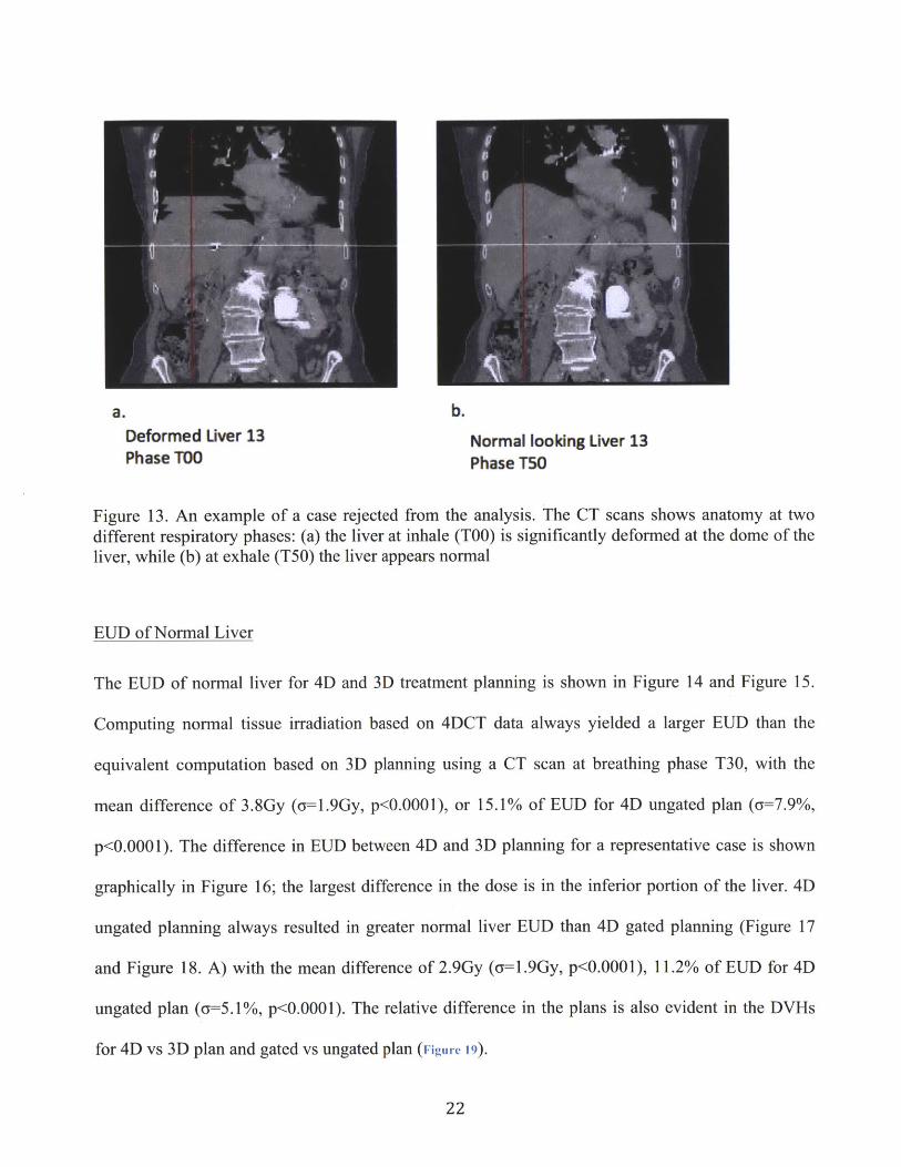
a. b.Deformed Liver 13 Normal looking Liver 13Phase TOO Phase T50

Figure 13. An example of a case rejected from the analysis. The CT scans shows anatomy at twodifferent respiratory phases: (a) the liver at inhale (TOO) is significantly deformed at the dome of theliver, while (b) at exhale (T50) the liver appears normal

EUD of Normal Liver

The EUD of normal liver for 4D and 3D treatment planning is shown in Figure 14 and Figure 15.

Computing normal tissue irradiation based on 4DCT data always yielded a larger EUD than the

equivalent computation based on 3D planning using a CT scan at breathing phase T30, with the

mean difference of 3.8Gy (a=1.9Gy, p<0.0001), or 15.1% of EUD for 4D ungated plan (a=7.9%,

p<0.0001). The difference in EUD between 4D and 3D planning for a representative case is shown

graphically in Figure 16; the largest difference in the dose is in the inferior portion of the liver. 4D

ungated planning always resulted in greater normal liver EUD than 4D gated planning (Figure 17

and Figure 18. A) with the mean difference of 2.9Gy (a=1.9Gy, p<0.0001), 11.2% of EUD for 4D

ungated plan (a=5.1%, p<0.0001). The relative difference in the plans is also evident in the DVHs

for 4D vs 3D plan and gated vs ungated plan (Figure 19).

22

4D vs 3D EUD

60

50 3

W40

w30

20

10

01 2 3 4 5 6 7 8 9 10 11 12 13 14 15 16 17 18 19 20 21 22 23 24 25

Liveor c ases

Figure 14. Comparison of 4D vs 3D treatment plan; the plot shows EUD [Gy] for 4D plan (gray) and3D plan (black) for 25 patients. 4D treatment planning results in a higher EUD to normal liver.

4D vs 3D AEUD

10 -9 -8 -

3

0 1 m r1 2 3 4 5 6 7 8 9 10 11 12 13 14 15 16 17 18 19 20 21 22 23 24 25

Liver cases

Figure 15. Difference between 4D and 3D treatment plan; the plot shows AEUD [Gy]= 4D EUD-3DEUD.

23

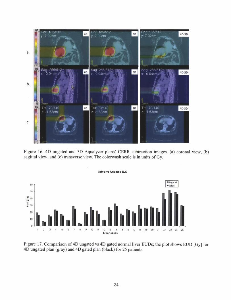
a.

b.

so4D 3D D3

C.

Figure 16. 4D ungated and 3D Aqualyzer plans' CERR subtraction images. (a) coronal view, (b)sagittal view, and (c) transverse view. The colorwash scale is in units of Gy.

Gated vs Ungated EUD

60[Ungated

MGat ed

50

40

0

20

10

0

1 2 3 4 5 6 7 8 9 10 11 12 13 14 15 16 17 18 19 20 21 22 23 24 25Liver cases

Figure 17. Comparison of 4D ungated vs 4D gated normal liver EUDs; the plot shows EUD [Gy] for4D ungated plan (gray) and 4D gated plan (black) for 25 patients.

24

A Gated vs Ungated delta EUD

'thdililhU~

I 2 3 4 6 1 L 1 1 4 3 It "?1 19 f 2. .2 11 24 J,

Liver cases

B Tumor motion distribution across liver cases

4

Liver cases

Tumor size distribution across the liver cases

iLi3 234 1 ?

.fli 1.h IN! HW 42 1D Ie11 13 1 4 14 E 37 31 35 2r 21 22 23 24 21

Liwer cases

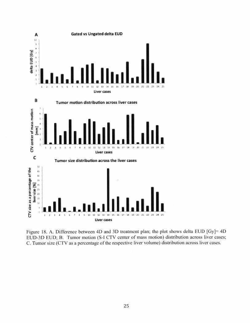
Figure 18. A. Difference between 4D and 3D treatment plan; the plot shows delta EUD [Gy]= 4DEUD-3D EUD; B. Tumor motion (S-I CTV center of mass motion) distribution across liver cases;C. Tumor size (CTV as a percentage of the respective liver volume) distribution across liver cases.

25

I

C

Gated Vs Ungated Vs 30 DVH for Llver-CTV

70

60

50

?40

E

30

20 Ungated

kGate

10 A 3D

00 10 20 30 40 50 60 70

Dose(Gy)

Figure 19. Comparison of cumulative DVH for 4D gated, ungated and for 3D plans for a

representative liver case. The liver irradiated volume is the greatest for 4D ungated plan and the

smallest for 3D plan.

Correlation between AEUD and Tumor Motion, Size and Position

A logical question to ask is if there is a correlation between the size of the change in EUD to normal

liver and variables such as tumor motion amplitude, tumor size, or tumor location within the liver.

These variables are plotted in Figure 18. B,C. Since no obvious conclusion could be reached by just

inspecting the data, we computed correlations between AEUD and CTV mean center of mass motion

and between AEUD and CTV size. A weak correlation was observed between AEUD and CTV

motion (r=0.59 for 4D/3D, r=0.48 for ungated/gated) and a much weaker correlation was observed

with CTV size (r=0.31 for 4D/3D, r=0.26 for ungated/gated), see

26

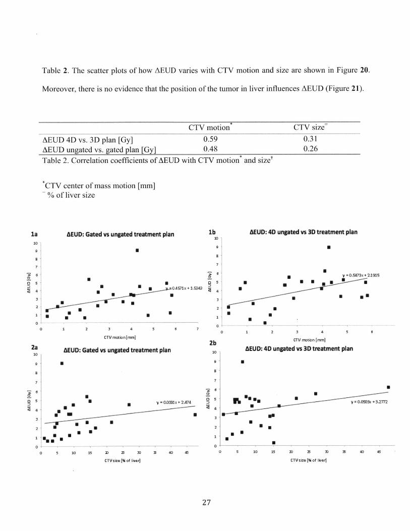
Table 2. The scatter plots of how AEUD varies with CTV motion and size are shown in Figure 20.

Moreover, there is no evidence that the position of the tumor in liver influences AEUD (Figure 21).

CTV motion* CTV size=

AEUD 4D vs. 3D plan [Gy] 0.59 0.31AEUD ungated vs. gated plan [Gy] 0.48 0.26Table 2. Correlation coefficients of AEUD with CTV motion* and size'

CTV center of mass motion [mm]% of liver size

AEUD: Gated vs ungated treatment plan

a

lb30~

:171

4'U 0-.4571 m+ 1.5343

3-2

1 2 3 4 5

CTV motion [mm]

AEUD: Gated vs ungated treatment plan

6

a

UU

U U v =OO~1s+2474

U U

I UU

* EU UU.. U

6

05

3

0

2b109-

7

(30

6

5-

4-

3-

2

0t I - - 1 1 1 - I .

0 5 10 15 2Z 2 30 3 40 45

CTVsize [% of liver]

AEUD: 4D ungated vs 3D treatment plan

a

UU V=O,54736+2.191S

U U U mmU

U mU

UU

U

0

SU

1 2 3 4 5 6

CTV rnotion [mm]

AEUD: 4D ungated vs 3D treatment plan

v .93 +327

UU

U

0 5 10 15 2D 25 3 3 40 45

CTVsize [% of liier]

27

la:10

7'

Q3

0

Za

7

0n4

3

0

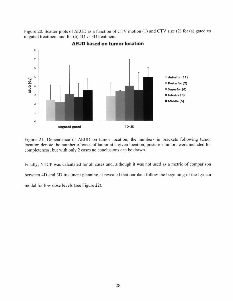
Figure 20. Scatter plots of AEUD as a function of CTV motion (1) and CTV size (2) for (a) gated vsungated treatment and for (b) 4D vs 3D treatment.

AEUD based on tumor location8

6

U,a

5

4

3

0

II

Anterior (11)

Posterior (2)

Superior (6)

* Inferior (8)

EMidde (5)

4D-3D

I

ungated-gated

Figure 21. Dependence of AEUD on tumor location; the numbers in brackets following tumorlocation denote the number of cases of tumor at a given location; posterior tumors were included forcompleteness, but with only 2 cases no conclusions can be drawn.

Finally, NTCP was calculated for all cases and, although it was not used as a metric of comparison

between 4D and 3D treatment planning, it revealed that our data follow the beginning of the Lyman

model for low dose levels (see Figure 22).

28

Normal liver NTCP as a function of dose5 -

4.5

4

3.5

3-

2.5

2

1.5

1 -

0.5 -

0 - .5 5.0 10 20 30 40 50 60 70

Dose prescribed [Gy]

Figure 22. NTCP as a function of the prescribed dose calculated before dose normalization to 60Gy.

DISCUSSION

Accurate assessment of radiation doses delivered to target as well as normal tissue is critical in safe

and effective radiation treatment. As shown in Figure 14,Figure 15, and Figure 16, dose distributions

and EUDs calculated by static 3DCT-based treatment planning significantly differ from those

computed by a 4D treatment planning. This finding is consistent with previous publications (20) and

motivates the use of 4DCT-based treatment planning to improve the ability to predict the doses

delivered to healthy liver tissue during the treatment.

Unlike Rosu et al (20), however, we found that static 3DCT-based planning always underestimates

the dose to normal liver independent of tumor position (Rosu et al reported that, compared to their

convolution-based mathematical model, for tumors in the superior liver static 3D planning

overestimates the normal liver dose while for tumors in the inferior liver, static planning

29

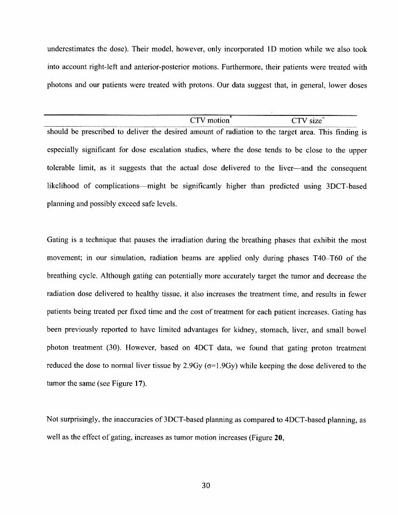
underestimates the dose). Their model, however, only incorporated 1 D motion while we also took

into account right-left and anterior-posterior motions. Furthermore, their patients were treated with

photons and our patients were treated with protons. Our data suggest that, in general, lower doses

CTV motion CTV sizeshould be prescribed to deliver the desired amount of radiation to the target area. This finding is

especially significant for dose escalation studies, where the dose tends to be close to the upper

tolerable limit, as it suggests that the actual dose delivered to the liver-and the consequent

likelihood of complications-might be significantly higher than predicted using 3DCT-based

planning and possibly exceed safe levels.

Gating is a technique that pauses the irradiation during the breathing phases that exhibit the most

movement; in our simulation, radiation beams are applied only during phases T40-T60 of the

breathing cycle. Although gatifig can potentially more accurately target the tumor and decrease the

radiation dose delivered to healthy tissue, it also increases the treatment time, and results in fewer

patients being treated per fixed time and the cost of treatment for each patient increases. Gating has

been previously reported to have limited advantages for kidney, stomach, liver, and small bowel

photon treatment (30). However, based on 4DCT data, we found that gating proton treatment

reduced the dose to normal liver tissue by 2.9Gy (G=1.9Gy) while keeping the dose delivered to the

tumor the same (see Figure 17).

Not surprisingly, the inaccuracies of 3DCT-based planning as compared to 4DCT-based planning, as

well as the effect of gating, increases as tumor motion increases (Figure 20,

30

AEUD 4D vs. 3D plan [Gy] 0.59 0.31AEUD ungated vs. gated plan [Gy] 0.48 0.26

Table 2). This makes sense because essentially the only difference between 4D and 3D planning is

that 4DTP takes into account the movement and 3DTP does not: thus, if the tumor moves more, 4D

planning accounts for more nonnal tissue that enters the beam's path during treatment. From a

clinical perspective, this finding suggests that, given limited resources, hospitals wishing to balance

patient volume and treatment quality might do so by prioritizing patients whose tumors move more

during breathing for more expensive 4DCT-based planning or gated treatment while using more

cost-effective 3DCT-based planning for patients whose tumors are relatively stationary.

As expected, the difference in EUD between 3DCT and 4DCT-based planning does not depend on

tumor size; because the primary difference between 3D and 4D planning is in the accounting for

tumor motion and not geometry, tumor size should not appreciably affect the EUD. On the other

hand, although we expected tumor location to matter (because the superior and middle regions of the

liver move more during breathing, and the inferior region moves least), the data available to us

consisted of too few cases data to be conclusive: although this trend can be visually noticed in Figure

21, no firm conclusions can be drawn because the standard deviations are too large.

EUD was chosen as the metric of comparison of 3D/4D and gated/ungated TP instead of the more

commonly used normal tissue complication probability (NTCP) (27) because for most of our

patients the doses to the liver were sufficiently low such that NTCP was close to 0 (see Figure 9). It

is impossible to compare NTCP differences if for both 3D and 4D NTCP was 0. NTCP is a threshold

metric and will stay at zero until a critical dose for a given fraction of liver irradiated is reached (as

31

shown in Figure 9), our NTCP computed values are at the beginning of the rise to the threshold

value. As a result, we chose EUD because it is derived from the DVH and hence provides a metric,

at the same time making the analysis much more straightforward. Both EUD and NTCP can be used

to optimize tumor treatment (31), hence choosing EUD does not decrease the clinical application of

our findings.

CONCLUSIONS

Because 3DCT-based radiation treatment planning does not account for tumor motion during

breathing, it inaccurately estimates the radiation dose delivered to normal tissue. In this study, we

have shown that 3D planning systematically underestimates the dose delivered to healthy liver tissue

by an average of 3.8Gy (c==1.9Gy) compared to doses estimated based on 4DCT data that treats each

breathing phase independently.

Gating the radiation beams during some breathing phases results in lower radiation exposure of

healthy tissue. Specifically, we found that applying treatment only during phases T40-T60 decreases

the dose to delivered to normal liver tissue by an average of 2.9Gy (Y=l.9Gy).

Future work will include looking at the effect of 4D planning as compared to 3D planning in a

different organ - the lung. The lung is interesting because of its very low density compared to other

tissues. As a result, the small changes in the dose planning are predicted to influence EUD to normal

organ (lung) much more than for liver. Besides, the lung moves, of course, during breathing which

will enable us to look at the effect of tumor motion in full swing.

32

REFERENCES

1. Trikalinos T, Terasawa T, Ip S, et al. Technical Brief on particle beam radiotherapies for thetreatment of cancer. Slide Presentation from the AHRQ 2010 Annual Conference September 2010

2. Bortfeld T. IMRT: a review and preview. Phys. Med Biol. 2006;51:pp.R363-3793. Gerber DE, Chan TA. Recent Advances in Radiation Therapy. Am Fain Physician 2008:78;pp.

1254-12624. Miller DW. A review of proton beam therapy. Med. Phys. 1995;22:pp. 1943-19545. Hauer-Jensen M. Late radiation injury of the small intestine: Clinical, pathophysiologic and

radiobiologic aspects-A review. Acta Oncologica 1990:29;pp. 401-4156. TomoTherapy. http://www.tomotherapy.com/beamlet/beamlet007/ Retrieved on 5/19/20117. Advanced Cancer Therapy. http://www.advanced-cancer-therapy.org/scienceproton.html

Retrieved on 5/19/20118. Pyakuryal A, Myint WK, Gopalakrishnan M, et al. A computational tool for the efficient analysis

of dose-volume histograms for radiation therapy treatment plans. JApplied Clinical Medical Phys2010; 11

9. Yorke E. Modeling the effects of inhomogeneous dose distributions in normal tissues. Seminars inRadiation Oncology 2001; 11:197-209

10. Dawson A, Hillen T. Derivation of the tumor control probability (TCP) from a cell cycle model.Journal of Theoretical Medicine 2006;00: 1-27

11. Gynecologic Oncology. http://www.mdconsult.com/books/page.do?eid=4-ul.0-B978-0-323-02951-3..50029-7&isbn=978-0-323-0295 1-3&type=bookPage&from=content&uniqld=248071062-26 Retrieved on 5/19/2011

12. Niemierko A. Reporting and analyzing dose distributions: A concept of equivalent uniform dose.Med Phys 1997;24:103-110

13. Pan CC, Kavanagh BD, Dawson LA, et al. Radiation-associated liver injury. Int JRadiat OncolBiol Phys 2010;76:S94-S100

14. McGinn CJ, Ten Haken RK, Ensminger WD, et al. The treatment of intrahepatic cancers withradiation doses based on a normal tissue complication probability model. J Clin Oncol1998; 16:2246-2252

15. Balter JM, Brock KK, Lam KL, et al. Evaluating the influence of setup uncertainties ontreatment planning for focal liver tumors. Int JRadiat Oncol Biol Phys 2005;63:610-614

16. Wu QJ, Meyer J, Fuller J, et al. Digital tomosynthesis for respiratory gated liver treatment:clinical feasibility for daily image guidance. Int JRadiat Oncol Biol Phys 2011;79:289-296

17. Kubas A, Chapet 0, Merle P, et al. Dosimetric impact of breath-hold in the treatment ofhepatocellular carcinoma by conformal radiation therapy [Impact dosimetrique du blocagerespiratoire dans le traitement du carcinome hepatocellulaire par irradiation de conformation].Cancer/Raadiotherapie 2009; 13:24-29

18. Wu QJ, Thongphiew D, Wang Z, et al. The impact of respiratory motion and treatment onstereotactic body radiation therapy for liver cancer. Medical Physics 2008;35:1440-1451

33

19. Coolens C, Evans PM, Seco J, et al. The susceptibility of IMRT dose distributions tointrafraction organ motion: an investigation into smoothing filters derived from four dimensionalcomputed tomography data. 2006;33:2809-2818

20. Rosu M, Dawson LA, Balter JM, et al. Alterations in normal liver doses due to organ motion. Int

JRadiat Oncol Biol Phys 2003;57:1472-147921. Wang X, Krishnan S, Zhang X, et al. Proton Radiotherapy for liver tumors: dosimetric

advantages over photon plans. Medical Dosimetry 2008;33:259-26722. Mori S, Chen GTY. Quantification and visualization of charged particle range variations. Int J

Radiat Oncol Biol Phys 2008;72:268-27723. Gustafsson A, Lind BK, Brahme A. A generalized pencil beam algorithm for optimization of

radiation therapy. Med Phys 1994;21:343-35624. Plastimatch. http://plastimatch.org. Retrieved on 4/12/201125. XIO Treatment Planning System. http://www.elekta.com/healthcareinternational-xio.php.

Retrieved on 5/18/201126. Deasy JO, Niemierko A, Herbert D, et al. Methodological issues in radiation dose - volume

outcome analyses: Summary of a joint AAPM/NIH workshop. Med Phys 2002;29:2109-212727. Dawson LA, Normolle D, Balter JM et al. Analysis of radiation-induced liver disease using the

Lyman NTCP model. Int JRadiat Oncol Biol Phys 2002;53:810-82128. Xio treatment planning. http://www.elekta.com/healthcareinternational xio.php29. Deasy JO, Blanco Al, Clark VH. CERR: A computational environment for radiotherapy

research. Med Phys 2003;30:979-98530. van der Geld YG, van Triest B, Verbakel WFAR, et al. Evaluation of four-dimensional

computed tomography-based Intensity Modulated and Respiratory-Gated RadiotherapyTechniques for Pancreatic Carcinoma. Int JRadiat Oncol Biol Phys 2008;72:1215-1220

31. Thomas E, Chapet 0, Kessler ML, et al. Benefit of using biologic parameters (EUD and NTCP)in IMRT optimization for treatment of intrahepatic tumors. Int J Radiat Oncol Biol Phys2005;62:571-578

32. Keall PJ, Joshi S, Sastry Vedam S, et al. Four-dimensional radiotherapy planning for DMLC-based respiratory motion tracking. Med Phys 2005;32:942-951

33. Urie M, Goitein M, Wagner M. Compensating for heterogeneities in proton radiation therapy.Phys Med Biol 1984;28:553-566

34

APPENDIX

Appendix A. Details of experimental treatment planning system - Aqualyzer.

Commercial proton treatment planning (e.g. CMS XIO used at MGH) does not have the capability ofperforming 4D dose calculations. Aqualyzer is a 4 dimensional treatment planning system for protonbeam therapy, written by Dr. Shinichiro Mori of the National Institute of Radiological Sciences,Chiba, Japan. The software development was begun when he was a postdoctoral fellow at MGH in2007. Aqualyzer is designed to calculate the dose for moving targets. The software is not FDAapproved, and therefore is not used for routine clinical use, but is used to better understand theimpact of motion on proton dose distributions.

Aqualyzer consists of two major components - Aqualyzer and Aquaview. The main functions ofAqualyzer are to a) read in 4D CT data b) read in contours drawn by the radiation oncologist on asingle phase of 4D CT data c) specify treatment parameters d) propagate these contours to all otherphases of respiration correlated CT data e) calculate a bolus for range compensation f) calculate doseat each respiratory phase g) map these distributions back to a single reference CT phase h) calculatethe composite dose and DVHs in the reference phase. The results are stored in a Results folder for agiven 4D calculation with specific input parameters. Aquaview's primary function is to data browsethrough the 4D dose distribution and aid in understanding 4D dose calculations.

Highlights of the specific steps in 4D treatment planning are provided to give an overview of what isinvolved in 4D treatment planning.

a) Reading in 4DCT: A folder containing the 10 phases of respiratory correlated CT is readinto Aqualyzer. The subfolders contain the CT slices at a specific phase, and are labeledT00, TO.....T90. T50 corresponds to exhale and TOO to inhale. Parts of the CT couch aresemi-automatically eliminated since they are not part of the treatment couch.

b) XIO contours of the target and organs at risk are read in. These contours are drawn by thephysician and treatment planner. For liver cases, typical contours segmented at T30include:

* GTV - the gross tumor volume - tumor visible on CT* CTV - the clinical target volume - an enlargement of the GTV, by an adequate

margin that includes microscopic extent (typically 5mm)- PTV - the planning target volume that includes an additional margin beyond the

CTV that accommodates inclusion of the target in the presence of setup errors andmotion.

e Critical structures such as the spinal cord, stomach, duodenum, entire liver, leftand right kidneys, porta hepatis, and any radio-opaque clips that are inserted nearthe edges of the tumor.

e Boolean structures can be generated in the contouring step. For example wedefine normal liver NLIV as the whole liver minus the CTV.

35

c) Specify treatment parameterse Beam direction: the user specifies which beam directions are to be used.

Typically, an anterior field and a right lateral field are used for proton beamtreatment of liver tumors. In some cases, the fields are obliqued to avoid ananatomical feature (e.g. an oblique field may avoid the GI tract, which the anteriorfield would hit). Occasionally a 3 field plan is used. Choice of field direction isbased on the experience of the dosimetrist and the physician's directive. Thebeam angles used in this analysis are the same as those used in the actual patienttreatment.

* Other treatment parameters are discussed belowd) Deformable image registration: 4D CT data contains lOx more image data than a

standard 3DCT. It is unrealistic to manually segment the target and normal anatomy for4D treatment planning. Therefore, Aqualzyer uses the software Plastimatch (24), writtenby Dr. Gregory Sharp of MGH. Plastimatch calculates the vector transformation from oneCT phase to another on a voxel by voxel basis. These transformations are then applied tothe manual contours of organs drawn by the physician, to "map" the contour to all otherphases of the respiratory correlated CT scan. This makes 4D treatment planning possible,since contours are needed at each phase for treatment planning. The end result of this stepis that one has a volumetric contour of each structure (e.g. target, right kidney) at eachrespiratory phase.

e) Calculate a bolus and aperture for a 4D structure: the strategy for designing acompensating bolus is to define it such that the target is always adequately irradiated. Notdoing so could lead to under-irradiation of the target during changes in radiologicpathlength during breathing. Therefore, a composite compensating bolus is designed fromthe 10 contours of the target. The bolus thickness chosen is the thinnest along a raythrough all 10 phases of CT data to the distal target from a given beam direction. Thisguarantees that in the presence of motion, the proton beam reaches the distal edge of thetarget. The union of the 10 targets in the beam's eye view plane ensures that the apertureis sufficiently large to cover the target should it move in the aperture plane. Typically a5mm range margin is used distally as a safety margin.

One additional parameter used in bolus design is important to point out. We include a"smearing" radius, typically 5-8mm. This smearing was originally suggested by Urie et al(33) as a way of ensuring target coverage in the event the compensating bolus and thetarget are misaligned during fractionated treatment. An exact nominal ray trace ensuresdistal range coverage with no uncertainty in bolus / target alignment. Smearing isachieved by choosing the thinnest radiological pathlength along neighboring rays withina 5mm/8mm radius. The smearing magnitude can be specified specifically along the xand y axes (z being along depth) should there the possibility of assymetric uncertainty.

Other treatment parameters:One can specify the width of the gating window. Our typical assumption is that gating isperformed in the T40-T60 window. This can be changed in the treatment parameterpanel.

36

Prescription dose in Gy may be specified. The DVHs and isodose distributions areususally displayed as percentages, 100% being normalized to the prescription dose.

Beam weight: relative dose contribution to isocenter is specified by this standardtreatment planning parameter.

f) Dose calculation at each phase: with the compensating bolus specified by the analysis oftarget motion in 10 phases, dose calculations at each phase are then performed. Thesoftware is designed to operate in a multi-cpu environment. Most calculations areperformed on a PC with a dual quad core processor. Dose calculations may require 1 hr.The end result is a set of 10 dose calculations, one for each respiratory phase. The dosedistributions at this point are called the "room's eye view" dose distributions, reflectingwhat one would see when both anatomy and dose move in the room coordinate system.

g) Mapping dose back to the reference CT phase: We map the dose distribution from eachrespiratory phase back to a reference phase (typically the phase on which the physiciandrew the target). This step reduces the graphical data spread over multiple spatialinstances to one spatial instance. The dose distribution in this space is called the"deformed dose". In this coordinate system, the anatomy is static, but the isodosedistribution varies with time. This is sometimes also referred to as the organ's eye view;it is somewhat analogous to being in a glass elevator. You may feel you are not moving,but see the floors pass by as the elevator moves up/down.

h) Finally, we integrate the moving dose distribution over time, resulting in the"accumulated dose distribution". The endpoint is a static, composite dose distributionover static anatomy. We can now proceed with calculation of a DVH for an organ, asdone in 3D treatment planning.

Miscellaneous:

Conversion from HU to water equivalent pathlength:

A CT scan provides a map of linear attenuation coefficients of the tissue relative to the linearattenuation coefficient of water at the nominal scan energy (effective x-ray energy). Both theelectron density and effective atomic number of the material (and photon energy) determine the u.On the other hand, dE/dx of a charged particle is primarily dependent on the electron density (with alogarithmic dependence on the atomic number). To map the CT scan to a map of electron densitiesthat is needed to calculate proton penetration, a simple calibration curve is used, as shown in FigureXX. In this figure, the y axis is the relative electron density, and the x-axis is the HU from the CTscan. Point of inflection is seen near OHU, and approximates the dependence on Z for tissues foundin the body.

Aquaview facilitates browsing through the several GB of data generated by Aqualyzer. These datainclude: a) composite and single field dose distributions in the room's eye view b) composite andsingle field dose distributions in the deformed (organ's eye) coordinate system and c) composite andsingle field distributions in the accumulated frame of reference. Aquaview also facilitates generationof movies to show dynamic dose distributions in the room and organ's eye view. It exports excelspreadheets of the dose volume histograms. These DVHs are then used to calculate the equivalentuniform dose (EUD) to tumor and normal tissues.

37

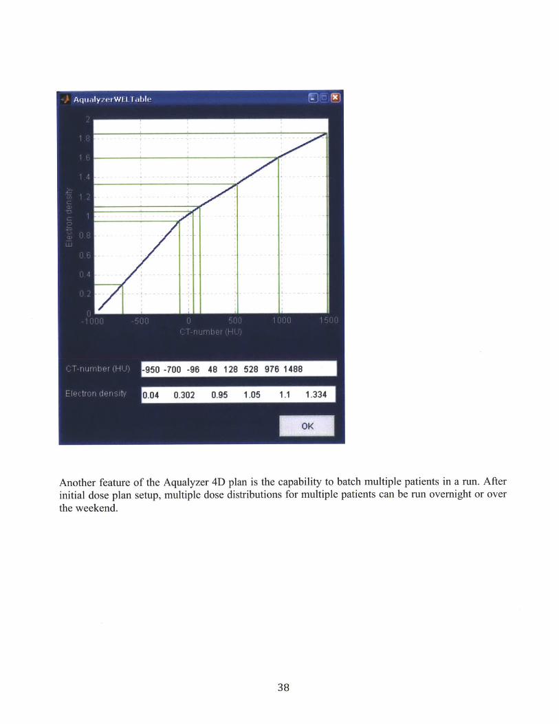
Another feature of the Aqualyzer 4D plan is the capability to batch multiple patients in a run. Afterinitial dose plan setup, multiple dose distributions for multiple patients can be run overnight or overthe weekend.

38

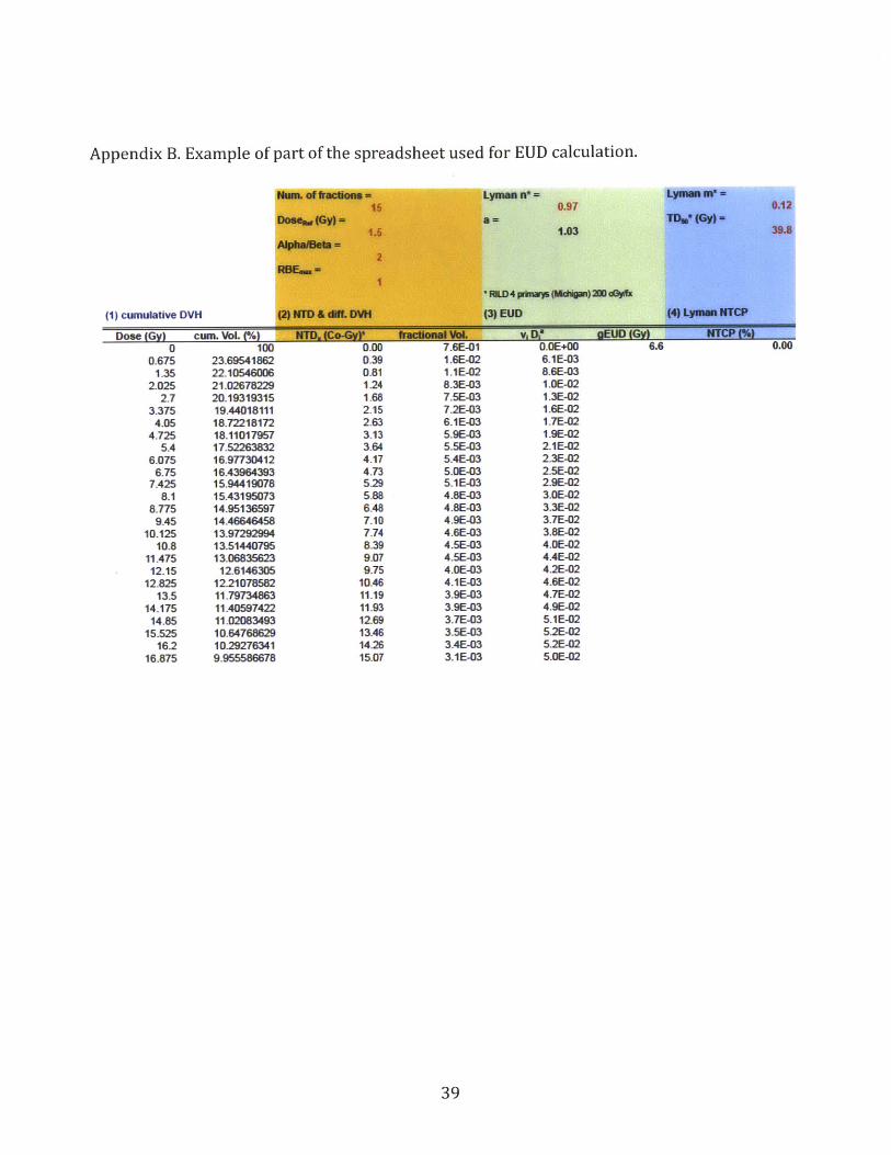
Appendix B. Example of part of the spreadsheet used for EUD calculation.

UM. Of *acumn yn s*e0.07

AlitlWt 4-~n &~)2 ~

(1) cumulative DVH M2 NftD & eMLa D13) EUD

Dose (Gy) cum Vol. (% V,(o-y rcics u gEU (Gy)0 100 0.00 7.6E-01 0.0E+00 6.6

0.675 23.69541862 0.39 1.6E-02 61E-031.35 22.10546006 0.81 1.1E-02 8.6E-03

2.025 21.02678229 1.24 8.3E-03 1.OE-022.7 20.19319315 1.68 7.5E-03 1.3E-02

3.375 19.44018111 2.15 7.2E-03 1.6E-024.05 18.72218172 2.63 6.1E-03 1.7E-02

4.725 18.11017957 3.13 5.9E-03 19E-025.4 17.52263832 3.64 5.5E-03 2.1E-02

6.075 16.97730412 4.17 5AE-03 2.3E-026.75 16.43964393 4.73 5.OE-03 25E-02

7.425 15.94419078 5.29 5.IE-03 29E-028.1 15.43195073 5.88 4.8E-03 3.OE-02

8.775 14.95136597 6.48 4.8E-03 3.3E-029.45 14.46646458 7.10 4.9E-03 3.7E-02

10.125 13.97292994 7.74 4.6EM03 3.8E-0210.8 13.51440795 8.39 4.5E-03 4.OE-02

11.475 13.06835623 9.07 4.5E-03 4AE-0212.15 12.6146305 9.75 4.OE-03 4.2E-02

12.825 12.21078582 10.46 4.1E-03 4.6E-0213.5 11.79734863 11.19 3.9E-03 4.7E-02

14.175 11.40597422 11.93 3.9E-03 4.9E-0214.85 11.02083493 12.69 3.7E-03 5.1E-02

15.525 10.64768629 13.46 3.5E-03 5.2E-0216.2 10.29276341 14.26 3.4E-03 5.2E-02

16.875 9.955586678 15.07 3.1E-03 5.OE-02

39