ANALYSIS AND IMPLEMENTATION OFPREDICTION MODELS FOR THE DESIGN

OF FIXED TERRESTRIALPOINT-TO-POINT SYSTEMS

a thesis submitted to

the graduate school of engineering and science

of bilkent university

in partial fulfillment of the requirements for

the degree of

master of science

in

electrical and electronics engineering

By

Polat Goktas

January, 2015

ANALYSIS AND IMPLEMENTATION OF PREDICTION MODELS

FOR THE DESIGN OF FIXED TERRESTRIAL POINT-TO-POINT

SYSTEMS

By Polat Goktas

January, 2015

We certify that we have read this thesis and that in our opinion it is fully adequate,

in scope and in quality, as a thesis for the degree of Master of Science.

Prof. Dr. Ayhan Altıntas (Advisor)

Prof. Dr. Ezhan Karasan

Assist. Prof. Dr. Satılmıs Topcu

Approved for the Graduate School of Engineering and Science:

Prof. Dr. Levent OnuralDirector of the Graduate School

ii

ABSTRACT

ANALYSIS AND IMPLEMENTATION OFPREDICTION MODELS FOR THE DESIGN OF FIXED

TERRESTRIAL POINT-TO-POINT SYSTEMS

Polat Goktas

M.S. in Electrical and Electronics Engineering

Advisor: Prof. Dr. Ayhan Altıntas

January, 2015

In this study, propagation link analysis and implementation of prediction

models for the design of fixed terrestrial point-to-point systems are aimed.

Different propagation models in the literature are examined as case studies and

comparisons are made. Rec. ITU-R P.530 Model is analyzed in detail. The worst

month link availability is investigated for terrestrial microwave LOS/NLOS radio

links operating in NATO Band 3+ (1350-2690 MHz) and NATO Band 4 (4400-

5000 MHz) frequency bands. The calculation of Bullington model of diffraction

loss is extended for LOS path case and determination of reflection points on

the terrain profile is improved. Several terrestrial microwave LOS/NLOS radio

links are analyzed using the propagation parameters such as TX (transmitter)

and RX (receiver) station coordinates, path length, frequency, antenna heights

above ground level, antenna gains, polarization, radio refractivity gradient, time

percentage, target SNR (Signal to Noise Ratio), bandwidth, digital terrain ele-

vation and climate data. The calculation of the received power with the effect

of the ground reflection is developed to calculate the fade margin in the defined

microwave LOS/NLOS radio links. Received power is calculated by taking into

consideration the attenuation due to rain and atmospheric gases, diffraction loss

and the effect of multipath fading due to reflection. The validity of the imple-

mentation of link analysis is justified by comparison with the commercial ATDI

ICS telecom software and the measurement data existing in the literature over

sample microwave LOS/NLOS radio links.

Keywords: Rec. ITU-R P.530, multipath fading, link availability, received power,

line-of-sight (LOS) and non line-of-sight (NLOS) microwave radio links.

iii

OZET

SABIT KARASAL NOKTADAN-NOKTAYASISTEMLERININ TASARIMI ICIN TAHMIN

MODELLERININ ANALIZI VE UYGULANMASI

Polat Goktas

Elektrik ve Elektronik Muhendisligi Bolumu, Yuksek Lisans

Tez Danısmanı: Prof. Dr. Ayhan Altıntas

Ocak, 2015

Bu calısmada, sabit karasal noktadan-noktaya sistemlerin tasarımı icin yayılım

tahmin modellerinin link analizi ve uygulanması amaclanmıstır. Literaturdeki

farklı yayılım modellerinin simulasyon calısması olarak incelenmesi ve karsılastır-

ması yapılmıstır. Detaylı olarak, ITU-R P.530 modeli analiz edilmistir. NATO

Band 3+ (1350-2690 MHz) ve 4 (4400-5000 MHz) frekans bandında calısan karasal

mikrodalga radyo LOS/NLOS (Gorus cizgisinin ustunde/altında) linkleri icin

yayılım mekanizmalarınn en kotu aydaki link kullanılabilirligi arastırılmıstır.

Kama kırınım kaybında, Bullington modeli hesabının LOS arazi icin genisletil-

mesi ve arazi hat profilindeki yansıma noktalarının bulunması gelistirilmistir. TX

(verici) ve RX (alıcı) istasyonların koordinat bilgileri, radyo linkin TX ve RX

istasyonlar arasındaki mesafesi, frekans, TX ve RX antenlerin yerden yuksek-

likleri ve kazancları, polarizasyon tipi, radyo kırılma indisi, zaman yuzdesi,

hedef SNR (sinyal gurultu oranı), bant genisligi, sayısal arazi yukseklik haritası

ve iklimsel veriler gibi yayılım parametreleri kullanılarak cesitli karasal mikro-

dalga LOS/NLOS radyo linkler icin analizler edilmistir. LOS/NLOS mikrodalga

radyo linklerinde sonumlenme kesintisini hesaplamak icin yerden yansımanın

etkisi ile alıcıdaki guc seviyesinin hesaplanması gelistirilmistir. Yagmur ve at-

mosferik gazlardan kaynaklanan zayıflama, yansımadan kaynaklanan cok yollu

sonumlenmenin etkisi ve kama kırınım kaybı dikkate alınarak alıcıdaki guc seviyesi

hesaplanmıstır. Link analizi uygulanmasının dogrulanması, ornek mikrodalga

LOS/NLOS radyo linklerinde ticari ATDI ICS telecom yazılımı ve literaturde yer

alan olcum verileri ile kıyaslanarak yapılmıstır.

Anahtar sozcukler : ITU-R P.530, cok yollu sonumlenme, link kullanılabilirligi,

alıcıdaki guc seviyesi, karasal gorus cizgisi ve ufuk otesi mikrodalga radyo linkleri.

iv

Acknowledgement

First and foremost, I would like to sincerely extend my greatest appreciation to

my supervisor, Prof. Dr. Ayhan Altıntas, for his guidance, constructive criticism,

advice and encouragement throughout my masters program.

It is a pleasure to express my special thanks to Prof. Dr. Ezhan Karasan

and Assist. Prof. Dr. Satılmıs Topcu for their invaluable contributions of this

thesis, and also for supplying significant resources for the development of this

thesis at Communication and Spectrum Management Research Center (ISYAM).

I would also like to thank Mr. Gokhan Moral for their cooperation and friendship.

I wish to thank all of my friends and family members for their continuous support

and encouragement.

I was personally supported by TUBITAK, through BIDEB 2228 scholarship.

v

Contents

1 INTRODUCTION 1

2 REVIEW OF MULTIPATH FADING MODELS 4

2.1 Overview of Multipath Fading Models . . . . . . . . . . . . . . . 4

2.1.1 Barnett-Vigants Model . . . . . . . . . . . . . . . . . . . . 5

2.1.2 Morita Model . . . . . . . . . . . . . . . . . . . . . . . . . 7

2.1.3 Rec. ITU-R P.530 Model . . . . . . . . . . . . . . . . . . . 8

2.2 Comparison of Multipath Fading Models . . . . . . . . . . . . . . 10

2.3 Case Studies for Multipath Fading Models . . . . . . . . . . . . . 13

3 PROPAGATION MECHANISMS ON TERRESTRIAL

MICROWAVE RADIO LINK 17

3.1 Atmospheric Effects on Propagation . . . . . . . . . . . . . . . . . 18

3.1.1 Attenuation due to Atmospheric Gases . . . . . . . . . . . 19

3.1.2 Attenuation due to Rain . . . . . . . . . . . . . . . . . . . 20

vi

CONTENTS vii

3.2 Diffraction Fading . . . . . . . . . . . . . . . . . . . . . . . . . . . 26

3.2.1 Single Knife-Edge Diffraction Model . . . . . . . . . . . . 26

3.2.2 Double Knife-Edge Diffraction Model . . . . . . . . . . . . 30

3.2.2.1 Deygout Method . . . . . . . . . . . . . . . . . . 31

3.2.2.2 Epstein-Peterson Method . . . . . . . . . . . . . 32

3.2.3 Multiple Knife-Edge Diffraction Model . . . . . . . . . . . 33

3.2.3.1 Delta-Bullington Method . . . . . . . . . . . . . 33

3.2.3.2 Proposed Diffraction Method . . . . . . . . . . . 36

3.3 Diffuse Reflection Loss . . . . . . . . . . . . . . . . . . . . . . . . 38

4 LINK ANALYSIS AND SIMULATION STUDIES 43

4.1 Link Power Budget . . . . . . . . . . . . . . . . . . . . . . . . . . 44

4.1.1 Free Space Loss . . . . . . . . . . . . . . . . . . . . . . . . 45

4.1.2 Received Power . . . . . . . . . . . . . . . . . . . . . . . . 46

4.1.3 Noise Power . . . . . . . . . . . . . . . . . . . . . . . . . . 46

4.1.4 Coherence Bandwidth . . . . . . . . . . . . . . . . . . . . 47

4.1.5 Fade Margin . . . . . . . . . . . . . . . . . . . . . . . . . . 48

4.1.6 Link Availability . . . . . . . . . . . . . . . . . . . . . . . 48

4.2 Path Profile and Simulation Studies . . . . . . . . . . . . . . . . . 49

4.2.1 Kazan-Elmadag Microwave R/L Case Study . . . . . . . . 51

CONTENTS viii

4.2.2 Fenertepe-Sazlıtepe Microwave R/L Case Study . . . . . . 55

4.2.3 Polatlı-Huseyingazi Microwave R/L Case Study . . . . . . 58

4.2.4 Dikmen-Polatlı Microwave R/L Case Study . . . . . . . . 62

5 VALIDATION AND COMPARISON OF RESULTS 65

5.1 Comparison with the ATDI ICS Telecom Software . . . . . . . . . 66

5.2 Experimental Validation of ITU-R Model for Terrestrial LOS/NLOS

Microwave Links . . . . . . . . . . . . . . . . . . . . . . . . . . . 69

6 CONCLUSION 73

A Effective Earth Radius 76

B Fresnel Zones 81

List of Figures

2.1 Barnett-Vigants atmospheric propagation conditions map for the

United States. . . . . . . . . . . . . . . . . . . . . . . . . . . . . . 6

2.2 Worldwide map of Barnett-Vigants atmospheric propagation con-

ditions. . . . . . . . . . . . . . . . . . . . . . . . . . . . . . . . . . 6

2.3 Refractivity gradient in the lowest 65 m of the atmosphere not

exceeded for 1% of the average year, dN1. . . . . . . . . . . . . . 9

2.4 Map of the world showing countries for which data are available

in the ITU-R database. . . . . . . . . . . . . . . . . . . . . . . . . 11

2.5 Cumulative distributions of error for the 239 links (including over-

land and overwater links) ITU-R P. 530-8 model (——); Barnett-

Vigants model(- - -); Morita model( –. –. –.). . . . . . . . . . . . 12

2.6 Terrain path profile of Fenertepe-Sazlıtepe microwave LOS radio

link (the blue curve and the red curve indicate the first Fresnel

zone and the 0.6 First Fresnel zone, respectively). . . . . . . . . . 14

2.7 Percentage of time that fade depth has exceeded in the worst

month for various multipath fading models, 1.350 GHz. . . . . . . 15

2.8 Percentage of time that fade depth has exceeded in the worst

month for various multipath fading models, 5 GHz. . . . . . . . . 16

ix

LIST OF FIGURES x

3.1 Specific attenuation due to atmospheric gases: atmospheric pres-

sure, 1013 hPa; temperature, 15o C; water vapour, 7.5 g/m3. . . . 20

3.2 Rain attenuation prediction procedure. . . . . . . . . . . . . . . . 22

3.3 Specific attenuation due to rain for Sarıyer-Maslak radio link. . . 23

3.4 Specific attenuation due to rain for Polatlı-Elmadag radio link. . . 23

3.5 Rain attenuation on terrestrial 5 GHz link as a function of vertical

polarization. . . . . . . . . . . . . . . . . . . . . . . . . . . . . . . 25

3.6 Rain attenuation on terrestrial 5 GHz link as a function of hori-

zontal polarization. . . . . . . . . . . . . . . . . . . . . . . . . . . 25

3.7 Shadowing of radio waves by an object. . . . . . . . . . . . . . . . 28

3.8 Illustration of different single knife-edge diffraction scenarios. (a)

NLOS path case and α1, α2 and v are positive, since h is positive

(b) LOS path case and α1, α2 and v are negative, since h is negative. 28

3.9 Knife-edge diffraction loss as a function of Fresnel knife-edge

diffraction parameter. . . . . . . . . . . . . . . . . . . . . . . . . . 29

3.10 Knife-edge diffraction loss as a function of normalized clearance. . 29

3.11 Deygout method geometry over the LOS line. . . . . . . . . . . . 32

3.12 Epstein-Peterson method geometry over the LOS line. . . . . . . . 33

3.13 Bullington method geometry over the LOS line. . . . . . . . . . . 36

3.14 Relative permittivity, εr and conductivity, σ (S/m) as a function

of frequency. . . . . . . . . . . . . . . . . . . . . . . . . . . . . . . 39

3.15 The geometry of the reflected propagation path. . . . . . . . . . . 41

LIST OF FIGURES xi

4.1 An illustration of a typical microwave radio link. . . . . . . . . . . 44

4.2 Location of sites used for microwave link simulations in Istanbul. . 50

4.3 Location of sites used for microwave link simulations in Ankara. . 50

4.4 Terrain path profile of Kazan-Elmadag microwave LOS radio link

(Frequency: 2 GHz, TX&RX Antenna Heights: 15 m a.g.l). . . . . 51

4.5 Terrain path profile of Polatlı-Huseyingazi microwave NLOS radio

link (Frequency: 1.35 GHz, TX&RX Antenna Heights: 35 m a.g.l). 58

4.6 Terrain path profile of Dikmen-Polatlı microwave NLOS radio link

(Frequency: 2.690 GHz, TX&RX Antenna Heights: 40 m a.g.l). . 62

5.1 Kazan-Elmadag microwave LOS radio link profile over terrain with

the terrain elevations above sea level adjusted for 4/3 effective

Earth radius curvature by the ATDI ICS telecom software. . . . . 66

5.2 Terrain path profile of the scenario 1 (Frequency: 5 GHz, TX

Antenna Height: 9.8 m a.g.l and RX Antenna Height: 4.6 m a.g.l). 70

5.3 Terrain path profile of the scenario 2 (Frequency: 2 GHz, TX

Antenna Height: 11.8 m a.g.l and RX Antenna Height: 35 m a.g.l). 70

5.4 Path loss for the scenario 1 as abtained during the measurements

and by using the Delta-Bullington diffraction method for the trans-

mitter antenna height of 9.8 m a.g.l. . . . . . . . . . . . . . . . . 71

5.5 Path loss for the scenario 2 as abtained during the measurements

and by using the Delta-Bullington diffraction method for the trans-

mitter antenna height of 11.8 m a.g.l. . . . . . . . . . . . . . . . . 72

LIST OF FIGURES xii

5.6 Path loss for the scenario 2 as abtained during the measurements

and by using the Delta-Bullington diffraction method for the trans-

mitter antenna height of 23.8 m a.g.l. . . . . . . . . . . . . . . . . 72

A.1 Variation of the ray curvature for different values of k. . . . . . . . 78

A.2 Polatlı-Elmadag microwave radio link profile over terrain with the

terrain elevations above sea level adjusted for 4/3 effective Earth

radius curvature. (the blue curve and the red curve indicate the

first Fresnel zone and the 0.6 first Fresnel zone, respectively). . . . 80

B.1 Geometrical concept of Fresnel zones. . . . . . . . . . . . . . . . . 83

B.2 An illustration of the first Fresnel zone radius. . . . . . . . . . . . 83

List of Tables

2.1 Error statistics for various multipath fading models in terms of

terrain-climatic grouping of the links. . . . . . . . . . . . . . . . . 11

2.2 Percentage of links with error not exceeded in certain ranges. . . . 12

2.3 Terrestrial link parameters for Fenertepe-Sazlıtepe propagation path. 14

2.4 Comparison of derived parameters for three multipath fading mod-

els on Fenertepe-Sazlıtepe microwave LOS radio link . . . . . . . 15

3.1 Path propagation parameters used in Rec. ITU-R P.530 and P.526. 18

3.2 Main parameters used for reflection case study. . . . . . . . . . . . 40

3.3 The values of conductivity and relative permittivity for different

types of ground at 2 GHz frequency. . . . . . . . . . . . . . . . . 41

3.4 Reflection case study results for different types of ground and ver-

tical polarization on Fenertepe-Sazlıtepe microwave LOS link. . . 41

3.5 Reflection case study results for different types of ground and hor-

izontal polarization on Fenertepe-Sazlıtepe microwave LOS link. . 42

4.1 The outage time per year allowed for given link availability. . . . . 49

xiii

LIST OF TABLES xiv

4.2 Terrestrial link parameters for Kazan-Elmadag microwave LOS ra-

dio link. . . . . . . . . . . . . . . . . . . . . . . . . . . . . . . . . 52

4.3 Results of link simulation as a function of vertical polarization on

Kazan-Elmadag terrestrial microwave LOS radio link. . . . . . . . 53

4.4 Results of link simulation as a function of horizontal polarization

on Kazan-Elmadag terrestrial microwave LOS radio link. . . . . . 54

4.5 Terrestrial link parameters for Fenertepe-Sazlıtepe microwave LOS

radio link. . . . . . . . . . . . . . . . . . . . . . . . . . . . . . . . 55

4.6 Results of link simulation as a function of vertical polarization on

Fenertepe-Sazlıtepe terrestrial microwave LOS radio link. . . . . . 56

4.7 Results of link simulation as a function of horizontal polarization

on Fenertepe-Sazlıtepe terrestrial microwave LOS radio link. . . . 57

4.8 Terrestrial link parameters for Polatlı-Huseyingazi microwave

NLOS radio link. . . . . . . . . . . . . . . . . . . . . . . . . . . . 59

4.9 Results of link simulation for both horizontal and vertical polar-

izations on Polatlı-Huseyingazi terrestrial microwave NLOS radio

link (by using only Delta-Bullington diffraction method). . . . . . 60

4.10 Results of predicted diffraction loss for three diffraction prediction

methods on Polatlı-Huseyingazi terrestrial microwave NLOS radio

link. . . . . . . . . . . . . . . . . . . . . . . . . . . . . . . . . . . 61

4.11 Results of predicted received power for three diffraction prediction

methods on Polatlı-Huseyingazi terrestrial microwave NLOS radio

link. . . . . . . . . . . . . . . . . . . . . . . . . . . . . . . . . . . 61

4.12 Terrestrial link parameters for Dikmen-Polatlı microwave NLOS

radio link. . . . . . . . . . . . . . . . . . . . . . . . . . . . . . . . 63

LIST OF TABLES xv

4.13 Results of link simulation for both horizontal and vertical polar-

izations on Dikmen-Polatlı terrestrial microwave NLOS radio link. 64

5.1 Terrestrial link parameters for Kazan-Elmadag terrestrial mi-

crowave LOS radio link (validation case study). . . . . . . . . . . 67

5.2 Results of link simulation as a function of vertical polarization on

Kazan-Elmadag terrestrial microwave LOS radio link (validation

case study). . . . . . . . . . . . . . . . . . . . . . . . . . . . . . . 68

5.3 Results of ATDI ICS telecom software on Kazan-Elmadag terres-

trial microwave LOS radio link. . . . . . . . . . . . . . . . . . . . 68

5.4 Selected measurement scenarios. . . . . . . . . . . . . . . . . . . . 69

5.5 System parameters at 2.0 GHz, 3.5 GHz and 5.0 GHz. . . . . . . 69

A.1 k factor values for different atmospheric refractive conditions. . . 79

Chapter 1

INTRODUCTION

In fixed point-to-point microwave radio links, the information is transmitted bet-

ween transmitting and receiving antennas by electromagnetic waves. The signal

strength of electromagnetic waves weakens during wave propagation through the

environment. The difference of signal strengths from transmitter to receiver sites

is called as propagation path loss. The major mechanisms in path loss are attenua-

tion due to atmospheric absorption, attenuation due to rain, diffraction loss due to

obstructions and multipath fading due to multipath arising from reflection points

along the terrain path profile in addition to the free space path loss. The fade

margin is derived from the link budget calculation, and this parameter is then

used to find the link availability in the terrestrial microwave LOS/NLOS radio

link. Link availability is the main design parameter for many fixed terrestrial mic-

rowave radio links.

In the literature, prediction models for deep-fading range of the multipath

fading distribution have been in existence for several years. Most of these have

been based on empirical fits of Rayleigh-type distributions (i.e., with slopes of

10 dB/decade) to the fading data for individual countries. The best known tech-

niques in this category are those of Morita [1] for Japan (actually a worst-season

technique), Barnett [2] and Vigants [3] for the United States. Olsen and Tjelta

paper [4,5] have presented detailed testing results for the ITU-R P.530-8 model [6]

1

on a 239-link database from 22 countries around the world in comparison with

the results for the leading regional methods still frequently used by some link de-

signers for worldwide applications (the Barnett-Vigants model [2] of the United

States and the Morita model [1] of Japan).

In this study, we have investigated the performance of various “Point-to-Point”

path loss models on terrestrial microwave LOS/NLOS radio links in NATO Band

3+ (1350-2690 MHz) and NATO Band 4 (4400-5000 MHz) frequency ranges.

A total of three multipath fading models, namely Barnett-Vigants [2,3], Morita [1]

and Rec. ITU-R P.530 [7] models have been reviewed with different terrestrial

link and geoclimatic parameters in a rural environment. All estimated results of

the considered models are compared with the Rec. ITU-R P.530 [7] model values.

The available signal power formulation at the receiver with the effect of the ground

reflection is developed in the terrestrial microwave LOS/NLOS radio links. Then,

we calculated the fade margin in order to find the link availability value.

In Chapter 2, we have made a comparative study between three commonly used

prediction models for the terrestrial microwave LOS/NLOS radio links: Barnett-

Vigants [2, 3], Morita [1] and Rec. ITU-R P.530 [7]. We have analyzed the link

unavailability as a function of various parameters such as frequency, fade margin

and path distance. In addition, we have compared the performance of the three

multipath fading models in terms of the total outage probability over the sample

microwave radio link.

Chapter 3 presents work on the evaluation of the Rec. ITU-R P.530 point-to-

point radiowave propagation prediction model [7]. Four main aspects are analy-

zed: attenuation due to atmospheric gases and rain, the signal attenuation due to

diffraction based on knife-edge obstruction, and multipath fading due to multi-

path arising from specular reflection points along the terrestrial microwave radio

links.

Chapter 4 describes the implementation of the above mentioned Rec. ITU-R

P.530 model [7], and includes simulation results and performance evaluations over

sample fixed terrestrial microwave LOS/NLOS radio links. Then, the values of

2

the total received power and fade margin are calculated in the defined terrestrial

microwave LOS/NLOS radio link. The impact of several sites and environmental

parameters are examined in the calculation of the total received power.

In Chapter 5, the implementation of link analysis is compared by using both

the commercial ATDI ICS telecom software [8] and the measurement data existing

in the literature [9,10] over sample fixed terrestrial microwave LOS/NLOS radio

links. Concluding remarks and future works are discussed in Chapter 6.

Appendix A provides an information about k factor values for different

atmospheric refractive conditions, and also indicates the calculation of the radio

refractivity, dN1 (N-units/km) that is point refractivity gradient in the lowest 65

m of the atmosphere not exceeded for 1% of an average year.

Appendix B gives an information about Fresnel zone and ellipsoid in order to

calculate the diffraction loss along the terrestrial microwave radio LOS/NLOS

link, and the clearance criteria is then defined in the terrestrial microwave

LOS/NLOS radio link. So, the direct path between the transmitter and receiver

sites needs a clearance above ground of at least 60% of the radius of the first

Fresnel zone to achieve free space propagation condition.

3

Chapter 2

REVIEW OF MULTIPATH

FADING MODELS

Propagation prediction models for the design of fixed terrestrial point-to-point

systems have been derived estimating the probability of outage and link availa-

bility over a period of time. This chapter focuses on reviewing multipath fading

models as adopted by different authors in the worldwide. This chapter is divided

into two sections. The first section summarizes multipath fading models taking

into account different geoclimatic and terrestrial link parameters. The second sec-

tion compares the performance of all multipath fading models in terms of total

outage probability over the sample fixed terrestrial microwave radio link.

2.1 Overview of Multipath Fading Models

Techniques for predicting the deep-fading range of the multipath fading distri-

bution have been available for several years. Three models are commonly used

to predict the worst month link unavailability in the terrestrial microwave LOS/

NLOS radio links as called Morita [1], Barnett-Vigants [2,3] models used respec-

tively in Japan, North America, and the worldwide Rec. ITU-R P.530 model [7].

4

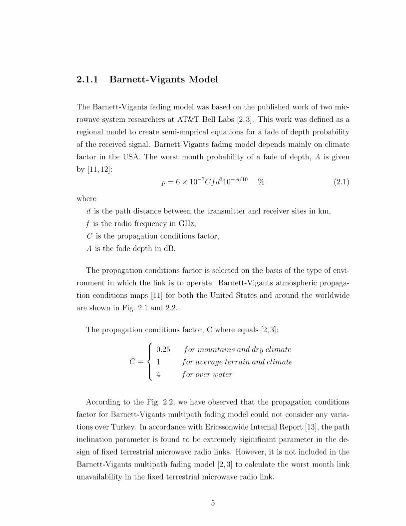
2.1.1 Barnett-Vigants Model

The Barnett-Vigants fading model was based on the published work of two mic-

rowave system researchers at AT&T Bell Labs [2, 3]. This work was defined as a

regional model to create semi-emprical equations for a fade of depth probability

of the received signal. Barnett-Vigants fading model depends mainly on climate

factor in the USA. The worst month probability of a fade of depth, A is given

by [11,12]:

p = 6× 10−7Cfd310−A/10 % (2.1)

where

d is the path distance between the transmitter and receiver sites in km,

f is the radio frequency in GHz,

C is the propagation conditions factor,

A is the fade depth in dB.

The propagation conditions factor is selected on the basis of the type of envi-

ronment in which the link is to operate. Barnett-Vigants atmospheric propaga-

tion conditions maps [11] for both the United States and around the worldwide

are shown in Fig. 2.1 and 2.2.

The propagation conditions factor, C where equals [2, 3]:

C =

0.25 for mountains and dry climate

1 for average terrain and climate

4 for over water

According to the Fig. 2.2, we have observed that the propagation conditions

factor for Barnett-Vigants multipath fading model could not consider any varia-

tions over Turkey. In accordance with Ericssonwide Internal Report [13], the path

inclination parameter is found to be extremely siginificant parameter in the de-

sign of fixed terrestrial microwave radio links. However, it is not included in the

Barnett-Vigants multipath fading model [2, 3] to calculate the worst month link

unavailability in the fixed terrestrial microwave radio link.

5

Figure 2.1: Barnett-Vigants atmospheric propagation conditions map for theUnited States.

Figure 2.2: Worldwide map of Barnett-Vigants atmospheric propagation condi-tions.

6

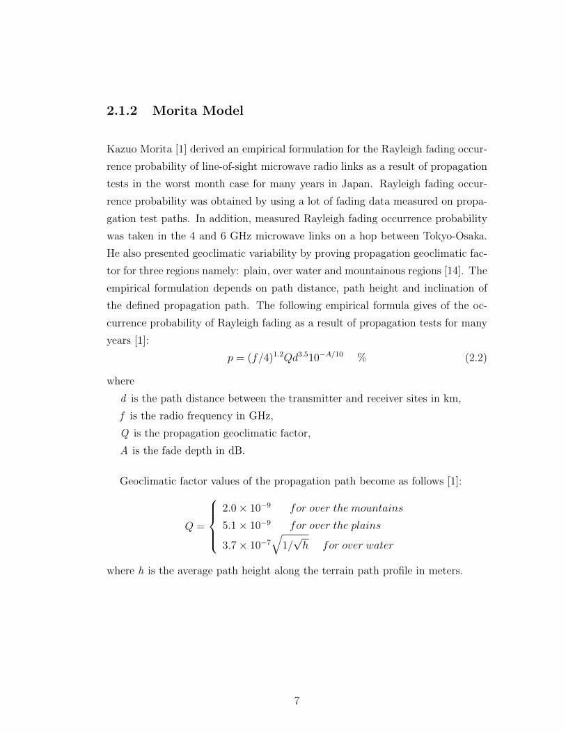
2.1.2 Morita Model

Kazuo Morita [1] derived an empirical formulation for the Rayleigh fading occur-

rence probability of line-of-sight microwave radio links as a result of propagation

tests in the worst month case for many years in Japan. Rayleigh fading occur-

rence probability was obtained by using a lot of fading data measured on propa-

gation test paths. In addition, measured Rayleigh fading occurrence probability

was taken in the 4 and 6 GHz microwave links on a hop between Tokyo-Osaka.

He also presented geoclimatic variability by proving propagation geoclimatic fac-

tor for three regions namely: plain, over water and mountainous regions [14]. The

empirical formulation depends on path distance, path height and inclination of

the defined propagation path. The following empirical formula gives of the oc-

currence probability of Rayleigh fading as a result of propagation tests for many

years [1]:

p = (f/4)1.2Qd3.510−A/10 % (2.2)

where

d is the path distance between the transmitter and receiver sites in km,

f is the radio frequency in GHz,

Q is the propagation geoclimatic factor,

A is the fade depth in dB.

Geoclimatic factor values of the propagation path become as follows [1]:

Q =

2.0× 10−9 for over the mountains

5.1× 10−9 for over the plains

3.7× 10−7√

1/√h for over water

where h is the average path height along the terrain path profile in meters.

7

2.1.3 Rec. ITU-R P.530 Model

Rec. ITU-R P.530 [7] is one of the most widely used model providing guidelines for

the design of terrestrial microwave LOS/NLOS radio links. A worldwide fading

model has been recommended by the Radiocommunication Sector of the Inter-

national Telecommunication Union (ITU-R) Study Group 3. The Study Group 3

of ITU has continued to revise the ITU-R P.530 models since the first version of

1978 [15, 16]. This recommendation is used to predict path losses in the average

worst month for terrestrial microwave LOS/NLOS radio links. The worst month

link unavailability depends on the impacts of both climate and terrain datas.

Two possible parameters are discussed below to calculate the geoclimatic factor

for the terrestrial microwave LOS/NLOS radio link.

Sa is defined as the standard deviation of terrain heights (m) within a 110 km

× 110 km area mentioned in Rec. ITU-R P.530. The worldwide data for this pa-

rameter is provided by ITU-R Study Group 3. The worldwide Sa data provided

by ITU-R is too coarse such that the distance between grid points is 110 km.

If the path length between transmitter and receiver sites is less than 110 km,

terrain roughness parameter is computed by using bi-linear interpolation at the

four closest gridpoints. The data provided by ITU-R Study Group 3 is also too

coarse to find the geoclimatic factor for the terrestrial microwave radio link [17].

The another required parameter is the radio refractivity gradient, dN1 that is

the point refractivity gradient in the lowest 65 m of the atmosphere not exceeded

for 1% of an average year. The radio refractivity parameter is provided on a 1.5

grid in latitude and longitude in Rec. ITU-R P.453 [18]. The refractivity gradient

in the lowest 65 m of the atmosphere, dN1 for the worldwide is shown in Fig. 2.3.

There are two ways to calculate geoclimatic factor parameter: a quick calcu-

lation (QC ) and a detailed link design (DLD) methods [7].

• The quick calculation (QC ) method uses only dN1, point refractivity gra-

dient parameter. The worst month outage probability, pw depends on the

geoclimatic factor of the quick calculation method according to Eq. (2.5).

8

Figure 2.3: Refractivity gradient in the lowest 65 m of the atmosphere not ex-ceeded for 1% of the average year, dN1.

ITU-R P.530-15 Fading Prediction Model

K=10−4.6−0.0027dN1 (2.3)

po = Kd3.1(1 + |εp|)−1.29f 0.8 × 10−0.00089hL (2.4)

pw = po× 10−A10 % (2.5)

• dN1 and Sa parameters are needed to calculate the geoclimatic factor of

the detailed link design (DLD) method. The percentage of time that fade

depth, A (in decibels) is exceeded in the average worst month calculated as:

K= 10−4.4−0.0027dN1(10+Sa)−0.46 (2.6)

po = Kd3.4(1+|εp|)−1.03f 0.8×10−0.00076hL (2.7)

pw = po× 10−A10 % (2.8)

9

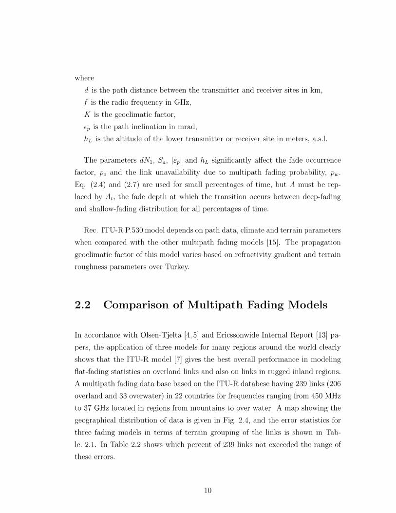
where

d is the path distance between the transmitter and receiver sites in km,

f is the radio frequency in GHz,

K is the geoclimatic factor,

εp is the path inclination in mrad,

hL is the altitude of the lower transmitter or receiver site in meters, a.s.l.

The parameters dN1, Sa, |εp| and hL significantly affect the fade occurrence

factor, po and the link unavailability due to multipath fading probability, pw.

Eq. (2.4) and (2.7) are used for small percentages of time, but A must be rep-

laced by At, the fade depth at which the transition occurs between deep-fading

and shallow-fading distribution for all percentages of time.

Rec. ITU-R P.530 model depends on path data, climate and terrain parameters

when compared with the other multipath fading models [15]. The propagation

geoclimatic factor of this model varies based on refractivity gradient and terrain

roughness parameters over Turkey.

2.2 Comparison of Multipath Fading Models

In accordance with Olsen-Tjelta [4, 5] and Ericssonwide Internal Report [13] pa-

pers, the application of three models for many regions around the world clearly

shows that the ITU-R model [7] gives the best overall performance in modeling

flat-fading statistics on overland links and also on links in rugged inland regions.

A multipath fading data base based on the ITU-R databese having 239 links (206

overland and 33 overwater) in 22 countries for frequencies ranging from 450 MHz

to 37 GHz located in regions from mountains to over water. A map showing the

geographical distribution of data is given in Fig. 2.4, and the error statistics for

three fading models in terms of terrain grouping of the links is shown in Tab-

le. 2.1. In Table 2.2 shows which percent of 239 links not exceeded the range of

these errors.

10

Figure 2.4: Map of the world showing countries for which data are available inthe ITU-R database.

Link Grouping N<E>(dB) σE (dB) RMS (dB) % |E −<E>|>10 (dB)

ITU-R US JPN ITU-R US JPN ITU-R US JPN ITU-R US JPNITU-R Inland 111 0.1 2.8 -12.1 5.2 6.6 7.7 5.3 9.4 19.8 3.6 12.6 13.5US Inland 104 0.0 2.4 -12.5 5.3 6.7 7.5 5.4 9.1 20.1 4.8 13.5 13.5JPN Island 122 0.1 2.7 -12.3 5.4 6.6 7.4 5.5 9.3 19.8 4.9 12.3 13.1ITU-R Mountainous 37 0.3 5.8 -6.6 6.2 8.2 8.2 6.4 14.1 14.9 8.1 21.6 21.6US/JPN Mountainous 44 0.7 6.3 -6.0 5.9 7.8 7.8 6.6 14.2 13.9 6.8 18.2 18.2ITU-R Coastal(medium-sized)

10 -2.2 2.3 -11.3 5.5 5.6 5.3 7.8 8.0 17.2 0.0 10.0 10.0

ITU-R Coastal (large) 38 0.1 2.4 -11.4 4.6 5.9 5.3 4.7 8.3 16.8 2.6 5.3 7.9ITU-R Coastal 58 -1.0 1.9 -11.8 4.9 5.6 5.1 5.9 7.6 16.9 3.5 6.9 6.9JPN Coastal 40 -1.9 0.8 -12.5 3.8 4.4 3.5 5.7 5.2 16.2 0.0 2.5 0.0ITU-R Overwater(medium-sized)

6 7.3 7.9 -1.9 5.4 6.1 6.8 13.4 14.8 8.9 0.0 0.0 0.0

ITU-R Overwater (large) 21 0.9 -0.8 -12.0 8.2 9.9 11.2 9.2 10.8 23.5 23.8 28.6 28.6ITU-R Overwater 27 2.4 1.1 -9.8 8.1 9.8 11.1 10.5 11.0 21.1 22.2 22.2 29.6ITU-R Coastal/Overwater(medium-sized)

16 1.4 4.4 -7.8 7.1 6.2 7.4 8.5 10.8 15.4 18.8 12.55 18.8

ITU-R Coastal/Overwater(large)

59 0.4 1..3 -11.6 6.1 7.6 7.8 6.5 8.9 19.5 8.5 11.9 15.3

ITU-R Coastal/Overwater 85 0.1 1.7 -11.2 6.2 7.2 7.5 6.3 8.9 18.7 10.6 12.9 15.3US Coastal/Overwater 84 0.0 1.6 -11.4 6.1 7.0 7.5 6.2 8.6 19.0 8.3 10.7 13.1JPN Coastal/Overwater 67 -0.2 1.0 -11.4 6.2 7.0 7.6 6.4 8.0 19.1 9.0 10.5 13.4High lat. (≥ 60o) 28 *0.3 0.8 -11.9 8.6 9.6 10.9 9.0 10.4 23.0 21.4 17.9 28.6All overland 206 -0.2 3.1 -11.0 5.3 6.8 7.4 5.5 9.9 18.4 5.3 15.1 16.5All 233 0.1 2.9 -10.9 5.7 7.2 7.9 5.8 10.1 18.8 6.9 15.9 18.0

Table 2.1: Error statistics for various multipath fading models in terms of terrain-climatic grouping of the links.

11

Figure 2.5: Cumulative distributions of error for the 239 links (including overlandand overwater links) ITU-R P. 530-8 model (——); Barnett-Vigants model(- - -);Morita model( –. –. –.).

ITU-RModel

Barnett-VigantsModel

MoritaModel

-5 dB to 5 dB 60 59 16-10 dB to 10 dB 93 83 36

Table 2.2: Percentage of links with error not exceeded in certain ranges.

According to Table. 2.1, ITU-R P.530 deep-fading distribution model has the

best mean error performance overall and for most terrain-climatic groupings.

On the other hand, the US (Barnett-Vigants) model overpredicts on average by

3.1 dB for all overland links, and the Japanese (Morita) model underpredicts

on average by 11 dB. So, Olsen-Tjelta [5] paper said that the US model was

developed for a range of latitudes below the average in the ITU-R database, and

Japanase model was developed for a very mountainous country.

In Fig. 2.5, we have observed that 90 percentage of 239 links in Morita model,

which predicted fade depth is smaller than measured fade depth with respect to

0 dB error criteria. 35 and 53 percent of 239 links in Barnett-Vigants model and

12

Rec. ITU-R P.530 model, which predicted fade depth is smaller than measured

fade depth with regards to 0 dB error criteria, respectively.

As depicted in Table 2.2, the prediction values of Rec. ITU-R P.530 model

are compatible with the measured values compared with the other multipath

fading models. So, Rec. ITU-R P.530 model gives the best overall performance

in modeling flat-fading statistics.

2.3 Case Studies for Multipath Fading Models

In this section, we have made case study simulation to compare results of three

multipath fading outage models over sample terrestrial microwave LOS radio link

located in Istanbul, Turkey. Fig. 2.6 shows the terrain path profile of Fenertepe-

Sazlıtepe microwave radio LOS link. Terrain and climate parameters for Fenerte-

pe-Sazlıtepe microwave LOS radio link are summarized in Table 2.3. We have

analyzed the worst month link unavailability as a function of the fade margin

with two different frequencies in NATO Band 3+ and 4 frequency ranges.

Comparison of derived parameters for three multipath fading outage models

on Fenertepe-Sazlıtepe propagation path is shown in Table 2.4. The three models

led to significantly different results for the link unavailability based on the fade

margin, frequency, link path length and geoclimatic factor parameters. At the fi-

xed link unavailability (pw= 10−3), fade margin can change up to 9.63 dB as

shown in Fig. 2.7 and 2.8. The fade margin difference between Rec. ITU-R P.530

and Barnett-Vigants models increases with the frequency while its variaton

between Morita and Rec. ITU-R P.530 models is slow with the frequency.

Rec. ITU-R P.530 model has more climate and terrain parameters to design

more accurate fixed terrestrial microwave radio LOS/NLOS links. So, there is

a flexibility K factor value due to dN1 and Sa parameters in contrast to Q and

C propagation conditions factor values which are solely based on generic tables.

It can be seen that Rec. ITU-R P.530 multipath fading mode is optimistic.

13

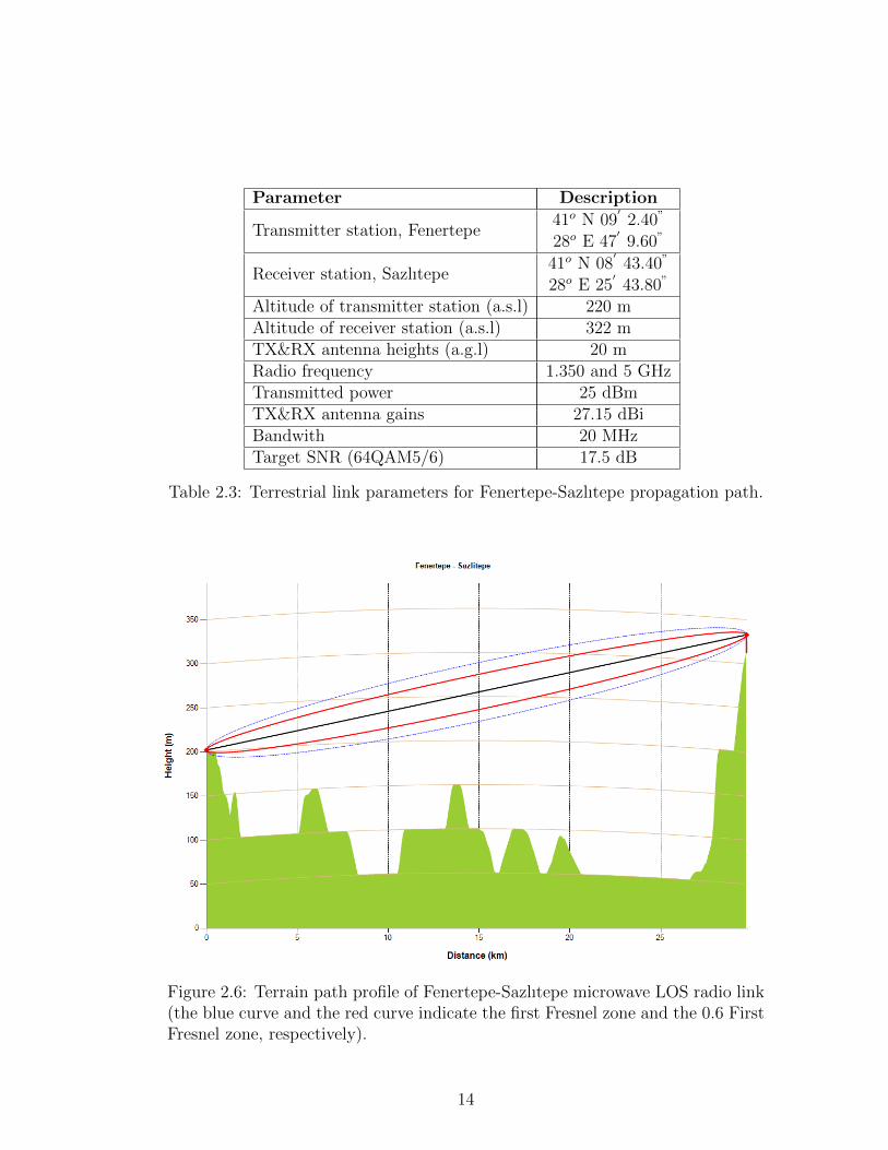
Parameter Description

Transmitter station, Fenertepe41o N 09

′2.40”

28o E 47′

9.60”

Receiver station, Sazlıtepe41o N 08

′43.40”

28o E 25′

43.80”

Altitude of transmitter station (a.s.l) 220 mAltitude of receiver station (a.s.l) 322 mTX&RX antenna heights (a.g.l) 20 mRadio frequency 1.350 and 5 GHzTransmitted power 25 dBmTX&RX antenna gains 27.15 dBiBandwith 20 MHzTarget SNR (64QAM5/6) 17.5 dB

Table 2.3: Terrestrial link parameters for Fenertepe-Sazlıtepe propagation path.

Figure 2.6: Terrain path profile of Fenertepe-Sazlıtepe microwave LOS radio link(the blue curve and the red curve indicate the first Fresnel zone and the 0.6 FirstFresnel zone, respectively).

14

Parameter DescriptionPath length 29.813 km

Path inclination 3.442 mraddN1

for Rec. ITU-R P.530 model-456.51 N-units/km

Safor Rec. ITU-R P.530 model

100.7 m

Geoclimatic factorfor Rec. ITU-R P.530 model

7.81× 10−5

Propagation conditions factorfor Barnett-Vigants model

2

Average path heightfor Morita model

96.09 m

Propagation geoclimatic factorfor Morita model

1.182× 10−7

Table 2.4: Comparison of derived parameters for three multipath fading modelson Fenertepe-Sazlıtepe microwave LOS radio link

Figure 2.7: Percentage of time that fade depth has exceeded in the worst monthfor various multipath fading models, 1.350 GHz.

15

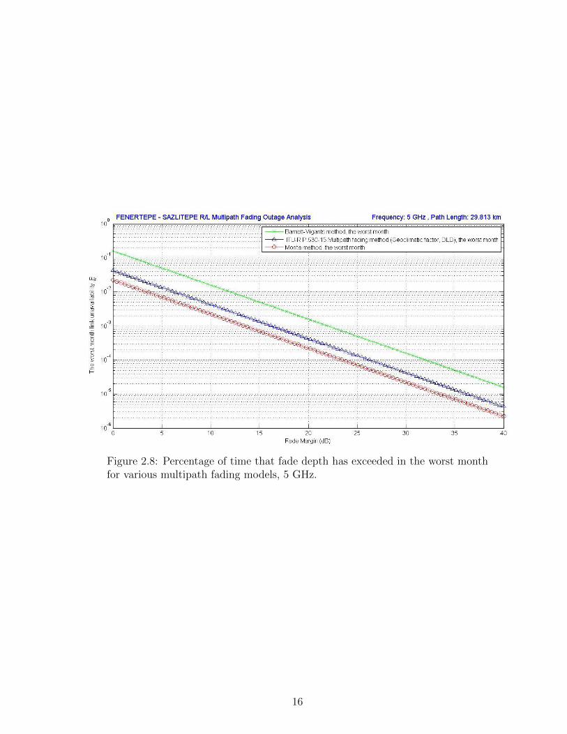
Figure 2.8: Percentage of time that fade depth has exceeded in the worst monthfor various multipath fading models, 5 GHz.

16

Chapter 3

PROPAGATION

MECHANISMS ON

TERRESTRIAL

MICROWAVE RADIO LINK

Rec. ITU-R P.530 path loss prediction model [7] is composed of four significant

clear-air and rainfall propagation mechanisms on the fixed terrestrial microwave

LOS/NLOS radio links: attenuation due to atmospheric gases and rain, fading

due to the multipath effects, and diffraction loss over terrain obstructions. This

chapter focuses on the characteristics of the propagation mechanisms in clear-air

and precipitation environments for terrestrial microwave LOS/NLOS radio links.

Table 3.1 summarizes Rec. ITU-R P.530 [7] and Rec. ITU-R P.526 [19] models

referring to path propagation on the fixed terrestrial point-to-point sytems. Dif-

ferent propagation mechnanisms are an important constraint on the prediction

of the path loss for terrestrial microwave LOS/NLOS radio links at different fre-

quencies. For frequencies below 5 GHz, attenuation due to atmospheric gases and

rain are small, and thus often neglected.

17

RECOMMENDATION ITU-R P.530 and P.526Application Fixed Terrestrial Microwave LOS/NLOS Radio Link

Type Point-to-Point Communication

Input

TX&RX Station Coordinates,TX&RX Antenna Heights (m, a.g.l),TX&RX Antenna Gains (dBi),TX Power (dBm),Path Length (km),Frequency (GHz),Percentage Time for Rain Attenuation (%),Polarization,SNR (dB),Bandwith (MHz),HPBW,Terrain Elevation Data,Climate Data.

Frequency 450 MHz-45 GHz

% timeAll percentage of time in clear-air conditions,0.001-1 in precipitation conditions.

Output

dN1, Radio Refractivity Gradient (N-units/km),Sa, Terrain Roughness (m),Rain Rate (mm/h),Free Space Loss (dB),Path Loss (dB),Total Received Power (dBm),Noise Power (dBm),Fade Margin (dB),Link Availability (%).

Table 3.1: Path propagation parameters used in Rec. ITU-R P.530 and P.526.

3.1 Atmospheric Effects on Propagation

In radio transmission, attenuation occurs due to two mechanisms: absorption

by atmospheric gases and rain. The attenuation due to absorption by atmo-

spheric gases is explicitly listed as an effect to be included in the link budget.

However, Rec. ITU-R P.530 does state: “On long paths at frequencies above

about 20 GHz, it may be desirable to take into account known statistics of water

vapour density and temperature in the vicinity of the defined path”. This state-

ment suggests that temporal variation of absorption fade may be significant at

these higher frequencies and on long paths. Moreover, attenuation due to rain is

much more significant at higher frequencies, especially above about 5 GHz.

18

3.1.1 Attenuation due to Atmospheric Gases

The transmission attenuation caused by atmospheric gases results from the mole-

cular resonance of oxygen and water vapour. An oxygen molecule has a single

permanent magnetic moment. At certain frequencies, its coupling with the mag-

netic field of an incident electromagnetic wave brings about resonance absorption.

So, the principal cause of signal attenuation due to atmospheric gases is molecular

absorption. Absorption by atmospheric gases depends on altitude above sea level,

frequency, temperature, pressure and water vapour concentration. Rec. ITU-R

P.676 [20] provides a method of calculating the specific attenuation with regards

to meteorological informations provided by Study Group 3. Fig. 3.1 shows that

specific attenuation from 1 to 350 GHz at sea-level for dry-air and water vapour

with density of 7.5 g/m3. At frequencies below 10 GHz, the excess attenuation

due to atmospheric gases is slightly under 0.01 dB/km so that the attenuation

due to atmospheric gases is insignificant in NATO Band 3+ and 4 frequency

bands. However, absorption becomes serious contributors to path loss above 10

GHz.

For longer paths, the attenuation due to atmospheric gases should be taken

into consideration in the calculation of the received signal power because the

attenuation is directly proportional to the length of the path. The atmospheric

attenuation on a path of length, d is given by [20,21]:

Agas = γtotald = (γo + γw)d (dB) (3.1)

where γo and γw are the specific attenuation due to oxygen and water vapour in

dB/km, respectively. In addition, γtotal is the total specific attenuation due to

atmospheric gases in dB/km.

19

Figure 3.1: Specific attenuation due to atmospheric gases: atmospheric pressure,1013 hPa; temperature, 15o C; water vapour, 7.5 g/m3.

3.1.2 Attenuation due to Rain

Attenuation due to rain is negligible at frequencies below 5 GHz. However, above

10 GHz, losses due to rain can cause outages, and it limits the availability of the

terrestrial microwave LOS/NLOS radio link. Rain attenuation prediction proce-

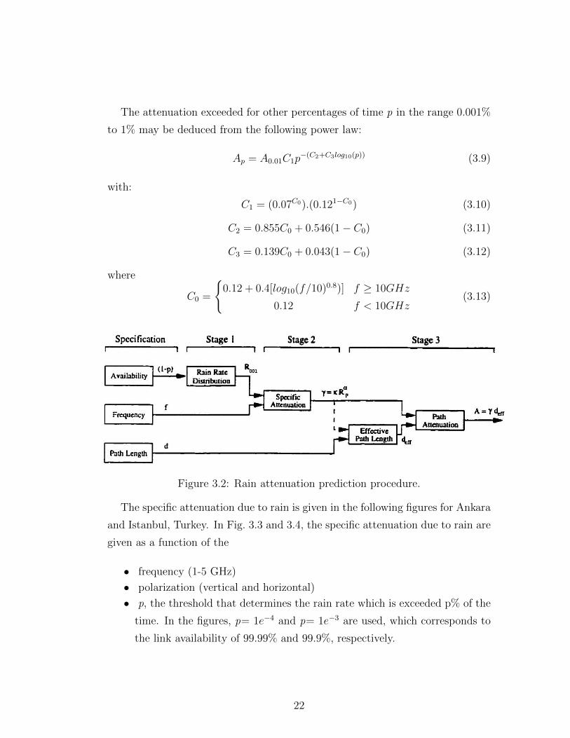
dure is shown in Fig. 3.2, and the rain attenuation is calculated in three stages.

The first stage, which estimates the rainfall rate at availability for 0.01%, re-

quires the knowledge of rain rate distributions which characterize the geographical

location of the defined microwave LOS/NLOS radio link. The rainfall rate excee-

ded for 0.01% of the time, R001% (mm/h) is computed by using the procedure

described in Rec. ITU-R P.837 [22].

20

In the second stage, specific attenuation due to rain in decibels per kilometer

depends on various parameters including rainfall rate, polarization and frequency.

The specific attenuation due to rain, γR (dB/km) is provided by Rec. ITU-

R P.838 [23], and obtained from the rainfall rate, R001% using the power law

relationship:

γR = kRα0.01% (3.2)

where k and α are frequency and polarization dependent coefficients. The coeffi-

cients can be determined using the following equations [23]:

log10kh|v =4∑j=1

aje−(

log10 f−bjcj

)2

+mk log10 f + ck (3.3)

αh|v =5∑j=1

aje−(

log10 f−bjcj

)2

+mα log10 f + cα (3.4)

Values for the constants required to calculate kh|v and αh|v are provided by

Rec. ITU-R P.838 [23]. The specific rain attenuation coefficient in Eq. (3.2) is

calculated from the values by Eqs. (3.3) and (3.4) using the following equations:

k = [kh + kv + (kh − kv)cos2(θ)cos(2τ)]/2 (3.5)

α = [khαh + kvαv + (khαh − kvαv)cos2(θ)cos(2τ)]/2k (3.6)

where θ is the path inclination and τ is the polarization tilt angle relative to the

horizontal.

At the last stage, an effective path length is estimated to account for the

rain inhomogeneous characteristic in the horizontal. The effective path length,

deff = r × d using the folowing equation [7]:

r =1

0.477d0.633R0.073×α0.01% f 0.123 − 10.579(1− e−0.024d)))

(3.7)

where d is the actual length of a radio link in km and r is the path reduction

factor.

Finally, multiplying the effective path length by the specific attenuation is

equal to the rain attenuation at 0.01% exceeded level, A0.01 (dB) is given by [7]:

A0.01 = γRdeff (3.8)

21

The attenuation exceeded for other percentages of time p in the range 0.001%

to 1% may be deduced from the following power law:

Ap = A0.01C1p−(C2+C3log10(p)) (3.9)

with:

C1 = (0.07C0).(0.121−C0) (3.10)

C2 = 0.855C0 + 0.546(1− C0) (3.11)

C3 = 0.139C0 + 0.043(1− C0) (3.12)

where

C0 =

{0.12 + 0.4[log10(f/10)0.8)] f ≥ 10GHz

0.12 f < 10GHz(3.13)

Figure 3.2: Rain attenuation prediction procedure.

The specific attenuation due to rain is given in the following figures for Ankara

and Istanbul, Turkey. In Fig. 3.3 and 3.4, the specific attenuation due to rain are

given as a function of the

• frequency (1-5 GHz)

• polarization (vertical and horizontal)

• p, the threshold that determines the rain rate which is exceeded p% of the

time. In the figures, p= 1e−4 and p= 1e−3 are used, which corresponds to

the link availability of 99.99% and 99.9%, respectively.

22

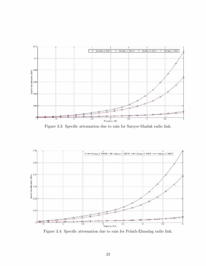
Figure 3.3: Specific attenuation due to rain for Sarıyer-Maslak radio link.

Figure 3.4: Specific attenuation due to rain for Polatlı-Elmadag radio link.

23

From Fig. 3.3 and 3.4, we make the following observations:

• The specific attenuation due to rain is negligible at frequencies below 5

GHz. However, the attenuation due to rain rapidly increases with frequency.

• The specific attenuation due to rain is considerably higher with horizontal

polarization compared with vertical polarization.

• Attenuation due to rain depends on rain rate with respect to the location.

i.e. the worst case of the path attenuation due to rain causes at 5 GHz,

p= 0.01% (corresponding to a link availability of 99.99%), and horizontal

polarization for Sarıyer-Maslak microwave LOS radio link.

The path attenuation due to rain as a function of path length varying between

1 and 50 km for the terrestrial microwave radio links are shown in the following

figures. These plots are obtained for the highest frequency, i.e., the worst case,

at 5 GHz and p= 0.01%, which corresponds to a link availability of 99.99%.

In Fig. 3.5 and 3.6, we have observed that the attenuation due to rain as a

function of both vertical polarization and a 50 km path ranges from 0.75 dB at

Ankara to nearly 1.1 dB at Istanbul. On the other hand, the attenuation due to

rain in horizontal polarization tended to be slightly larger than that in vertical

polarization for longer path at Istanbul, Turkey.

24

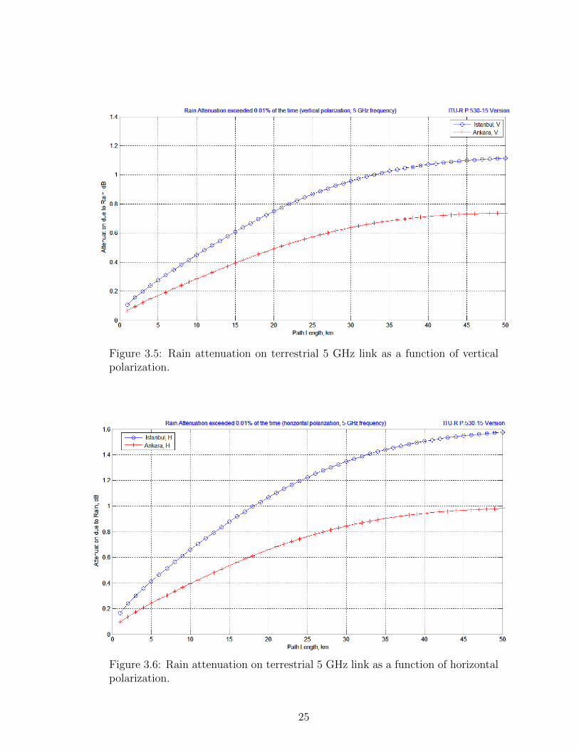
Figure 3.5: Rain attenuation on terrestrial 5 GHz link as a function of verticalpolarization.

Figure 3.6: Rain attenuation on terrestrial 5 GHz link as a function of horizontalpolarization.

25

3.2 Diffraction Fading

Diffraction phenomenon occurs when 60% of the first Fresnel zone is obstructed

by an obstacle or several obstacles between the transmitter and receiver sites.

To make the calculation of the diffraction loss, it is necessary to identify the form

of the obstacles assuming a knife-edge of negligible thickness. Diffraction loss de-

pends on the heights of hilltops with respect to the heights of the transmitter

and receiver sites taking into account the effective Earth radius related to ray-

path bending in the atmosphere, and the horizontal distances of the terrain path

profile points from the transmitter site.

Diffraction fading is based on the Huygen’s principle where each point of a

wavefront represents an infinite secondary source of a new spherical wave [24].

The wavelets above the obstacle propagation to all directions include the sha-

dowed area behind the obstacle. An illustration of shadowing of radio waves by

an object is found in Fig. 3.7.

3.2.1 Single Knife-Edge Diffraction Model

If the direct line-of-sight path is obstructed by a single knife-edge type of obs-

tacle as illustrated in Fig. 3.8, height of the top of the obstacle above the straight

line joining the two ends of the path, h. The knife-edge diffraction parameter is

defined as [19]:

v = h

√2(d1 + d2)

λd1d2(3.14)

v = θ

√2d1d2

λ(d1 + d2)(3.15)

v =

√2dα1α2

λ(3.16)

26

where d1 and d2 are the terminal slant distances from the knife-edge obstacle in

km, θ is angle of diffraction in radians, α1 and α2 are angles in radians between

the top of the obstacle and one end as seen from the other end. α1 and α2 are

of the sign of h in the above equations. Hence, the phase difference is written

as [19]:

φ =πv2

2(3.17)

Therefore, the total sum of contributions up to v as the complex Fresnel integ-

ral is written as [19]:

F (v) =

∫ v

0

ejπt2

2 dt = C(v) + jS(v) (3.18)

where

C(v) =

∫ v

0

cos(πt2

2)dt, S(v) =

∫ v

0

sin(πt2

2)dt (3.19)

The electric field strength, Ek, of a knife-edge diffracted wave is given by:

Ek =

∫ ∞v

ejπt2

2 dt (3.20)

Assuming that the value of the Cornu spiral for infinity is 0.5 + j0.5.

The field strength, Ek is then expressed using the finite integral:

Ek = (0.5 + j 0.5)−∫ v

0

ejπt2

2 dt = [0.5− C(v)] + j [0.5− S(v)] (3.21)

The electric field strength relative to free space is given by [19]:

Efield =EkEo

=

√[1 + C(v)− S(v)]2 + [C(v)− S(v)]2

2(3.22)

For the purposes of simplification in Rec. ITU-R P.526 [19], the diffraction

loss is calculated by the following formula:

Adiff (dB) =

{6.9 + 20log(

√(v − 0.1)2 + 1 + v − 0.1) v > −0.78

−20log(Efield) others(3.23)

27

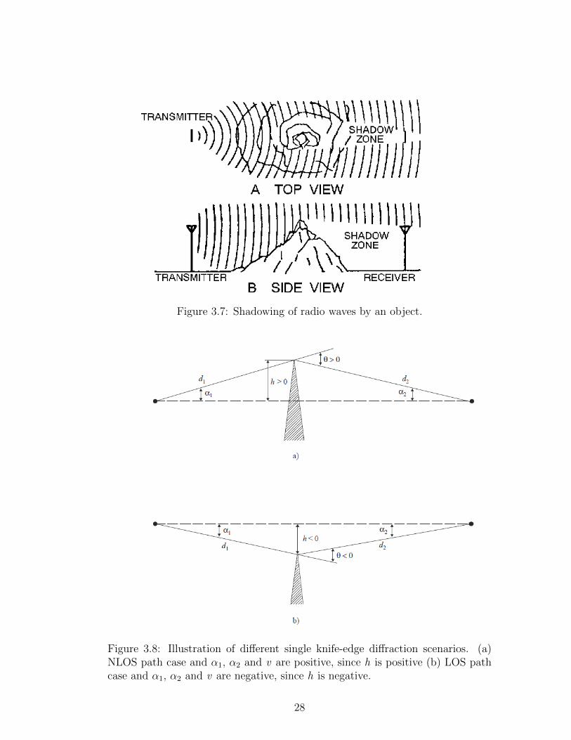
Figure 3.7: Shadowing of radio waves by an object.

Figure 3.8: Illustration of different single knife-edge diffraction scenarios. (a)NLOS path case and α1, α2 and v are positive, since h is positive (b) LOS pathcase and α1, α2 and v are negative, since h is negative.

28

Figure 3.9: Knife-edge diffraction loss as a function of Fresnel knife-edge diffrac-tion parameter.

Figure 3.10: Knife-edge diffraction loss as a function of normalized clearance.

29

In addition, an approximate solution for Eq. (3.23) provided by Lee [25] is

given by the following formula:

Loss(dB) =

0 v ≤ −1

20log(0.5− 0.62v) −1 ≤ v 6 0

20log(0.5e−0.95v) 0 ≤ v 6 1

20log(0.4−√

0.1184− (0.38− 0.1v)2) 1 ≤ v 6 2.4

20log(0.255v

) v > 2.4

(3.24)

In Fig. 3.9 and 3.10, comparison of an exact and approximation solution for

the diffraction loss due to the presence of a single knife-edge are made. If Fresnel

knife-edge diffraction parameter is smaller than -0.84 or clearance is smaller than

-0.6F1, the appearing blockage between transmitter and receiver sites can be

insignificant on the Fresnel ellipsoid zone. So, the direct path between transmitter

and receiver sites needs a clearance above ground of at least 60% of the radius of

the first Fresnel zone to ignore the effect of the diffraction loss.

3.2.2 Double Knife-Edge Diffraction Model

In many practical situations, especially in hilly terrain environment, the propa-

gation path consists of more than one obstruction in which case the diffraction

loss due to all of the obstacles must be computed. These effects are gene-

rally estimated using: (i) the classical prediction models proposed by Bulling-

ton, Deygout and Epstein-Peterson [26–28], with modifications; (ii) the ones

described by the most recent versions of Recommendations ITU-R P.526 [19].

In that case of two obstacles, the diffraction loss is calculated over the LOS

line (trans-horizon path type) whereby using the different prediction methods:

(i) Deygout, (ii) Epstein-Peterson and (iii) Delta-Bullington. The primary limi-

tation of Deygout and Epstein-Peterson diffraction methods is that correction

terms are not defined for the multiple knife-edge case mentioned in Rec. ITU-R

P.526. So, these diffraction prediction methods are only used for two obstacles

over the LOS line.

30

3.2.2.1 Deygout Method

This method consists of applying single knife-edge diffraction theory succes-

sively to the two obstacles along the terrestrial microwave NLOS radio link.

The first step in the Deygout method is choosing a dominant edge, which is

the obstacle with the highest Fresnel diffraction parameter. The main diffraction

loss caused only by the dominant obstacle and is then summed with the loss

from other obstacle whose height is given by the line between the transmitter or

receiver site and the top of the dominant edge. Fig 3.11 shows the construction

for an approximate calculation of the double knife-edge diffraction loss proposed

by Deygout [19].

In Fig. 3.11, the first edge is predominant and the first diffraction path is

defined by the distances a and b + c, and the clearance h1, gives a diffraction loss

L1 (dB). The second diffraction path is defined by the distances b and c, and the

clearance h′2, gives a loss L2 (dB). L1 and L2 are calculated by using formula of

Eq. (3.23).

A diffraction correction term, Correction(dB) [19], is calculated by using

Eq. (3.25), and then must be subtracted over the total diffraction loss to take

into account the separation between the two edges as well as their height.

Correction = [12− 20log(2

1− aπ

)](q

p)2p (dB) (3.25)

where

p = [2

λ

d

(b+ c)a]0.5h1 (3.26)

q = [2

λ

d

(a+ b)c]0.5h2 (3.27)

α = arctan(bd

ac)0.5 (3.28)

d = a+ b+ c (km) (3.29)

Finally, the total diffraction loss is calculated as [19]:

L = L1 + L2 − Correction (dB) (3.30)

31

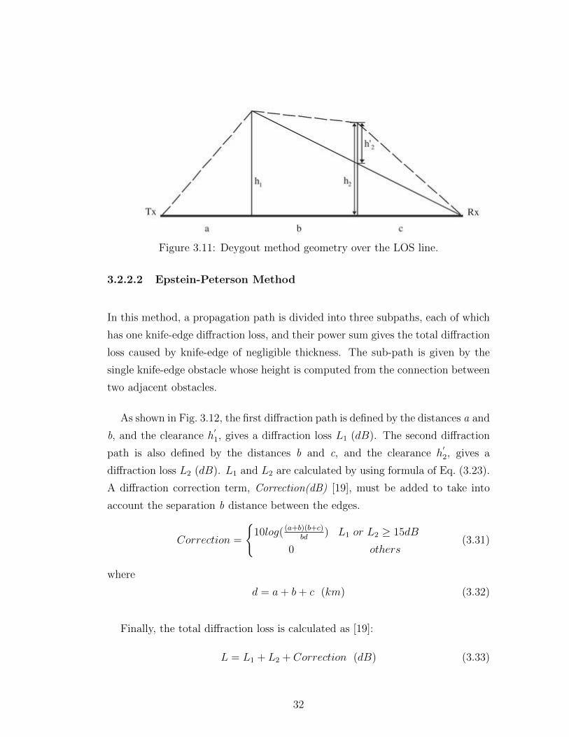
Figure 3.11: Deygout method geometry over the LOS line.

3.2.2.2 Epstein-Peterson Method

In this method, a propagation path is divided into three subpaths, each of which

has one knife-edge diffraction loss, and their power sum gives the total diffraction

loss caused by knife-edge of negligible thickness. The sub-path is given by the

single knife-edge obstacle whose height is computed from the connection between

two adjacent obstacles.

As shown in Fig. 3.12, the first diffraction path is defined by the distances a and

b, and the clearance h′1, gives a diffraction loss L1 (dB). The second diffraction

path is also defined by the distances b and c, and the clearance h′2, gives a

diffraction loss L2 (dB). L1 and L2 are calculated by using formula of Eq. (3.23).

A diffraction correction term, Correction(dB) [19], must be added to take into

account the separation b distance between the edges.

Correction =

{10log( (a+b)(b+c)

bd) L1 or L2 ≥ 15dB

0 others(3.31)

where

d = a+ b+ c (km) (3.32)

Finally, the total diffraction loss is calculated as [19]:

L = L1 + L2 + Correction (dB) (3.33)

32

Figure 3.12: Epstein-Peterson method geometry over the LOS line.

3.2.3 Multiple Knife-Edge Diffraction Model

If the propagation path consists of more than a single obstruction along the

path profile, Rec. ITU-R P.526 model provides Epstein-Peterson, Deygout and

Delta-Bullington methods to predict the total diffraction loss due to multiple

knife-edges, but the Epstein-Peterson and Deygout diffraction prediction met-

hods used only for two obstacles over the LOS line. In addition, if none of

the knife-edges are above the LOS line, then Rec. ITU-R P.526 suggests only

Delta-Bullington method on the calculation of the diffraction loss. For this case,

Delta-Bullington method is not based on constructing an equivalent hypothetical

single knife-edge at the intersection of transmitter and receiver sites because the

actual terrain profile point with the highest Fresnel diffraction parameter is found

along the terrain path profile. Alternatively, the modified Bullington model has

been proposed for supporting the Bullington construction in LOS path case.

3.2.3.1 Delta-Bullington Method

Delta-Bullington method has three parts as shown below:

• 1. Actual terrain profile and antenna heights above sea level are used to

calculate the Bullington diffraction loss, Lb(dB).

• 2. A smooth surface profile consists of the modified antenna heights at

the transmitter and receiver sites, and setting all other profile point hi to

33

zero. Bullington method is again applied for this smooth surface terrain

profile to calculate the diffraction loss, Lbs(dB). So, the Bullington part of

Delta-Bullington method is used twice.

• 3. The modified antenna heights of the smooth surface at the transmitter

and receiver sites, electrical characteristics of the surface of the Earth, and

equivalent Earth’s radius are input to the spherical-Earth diffraction model.

The predicted spherical-Earth diffraction loss is Lsph(dB).

In the following equations are related to the Bullington part of Delta-Bul-

lington method. The distance and height of the i -th profile point are di (km) and

hi (m, above sea level) respectively, i takes values from 1 to n where n is the

number of profile points. Transmitter and receiver heights are htx and hrx (m,

above sea level) respectively, and the complete path length is d (km). Effective

Earth curvature Ce (1/ km) is given by 1/ re where re is effective Earth radius

in km.

This method replaces several obstacles over the LOS line by one single knife-

edge obstacle whose height is given by the intersection of lines: the dominant

clearance profile point from transmitter site to receiver site is shown in Fig 3.13.

Firstly, the dominant profile point with the highest slope of the line from the

transmitter to the i -th profile point is given by [19]:

Stim = max[hi + 500Ced(d− di)− htx

di] (mrad) (3.34)

The slope of the LOS line from transmitter to receiver is calculated as [19]:

Str =hrx − htx

d(mrad) (3.35)

Two path cases are classsified as shown below:

Path Type =

{LOS Stim 6 Str

Transhorizon Stim > Str(3.36)

34

Case 1. Path Profile is LOS

This model is not based on constructing an equivalent hypothetical single knife-

edge at the intersection of transmitter and receiver sites, but the profile point with

the highest Fresnel diffraction parameter, vmax is found along the terrain path

profile.

vmax = max[hi + 500Ced(d− di)−htx(d− di) + hrxdi)

d]

√0.002d

λdi(d− di)(3.37)

In this case, the excess loss of the profile point is calculated as [19]:

Lknife(dB) =

{6.9 + 20log(

√(vmax − 0.1)2 + 1 + vmax − 0.1) vmax > −0.78

0 others

(3.38)

Case 2. Path Profile is Transhorizon

The dominant profile point with the highest slope of the line from the receiver

to the i -th profile point is given by [19]:

Srim = max[hi + 500Ced(d− di)− hrx

d− di] (mrad) (3.39)

One hypothetical knife-edge obstacle is defined by the intersection of Stim and

Srim. The distance of an equivalent knife-edge obstacle from the transmitter site

is given by [19]:

deq =hrx − htx + Srimd

Stim + Srim(mrad) (3.40)

Calculation of the Fresnel diffraction parameter, veq for an equivalent knife-

edge obstacle is given by [19]:

veq = [htx + Stimdeq −htx(d− deq) + hrxdb)

d]

√0.002d

λdeq(d− deq)(3.41)

In this case, the excess loss of an equivalent knife-edge obstacle is calculated

as:

Lknife(dB) =

{6.9 + 20log(

√(veq − 0.1)2 + 1 + veq − 0.1) veq > −0.78

−20log(F ) others(3.42)

35

where

F =

√[1 + C(veq)− S(veq)]2 + [C(veq)− S(veq)]2

2(3.43)

The diffraction loss is calculated by using either Eqs. (3.38) or (3.42), and

Bullington diffraction loss with the correction term is given by [19]:

Lb = Lknife + [1− e−Lknife

6 ](10 + 0.02d) (dB) (3.44)

The overall diffraction loss of the terrain path profile is calculated as [19]:

L = Lb +max(Lsph − Lbs, 0) (dB) (3.45)

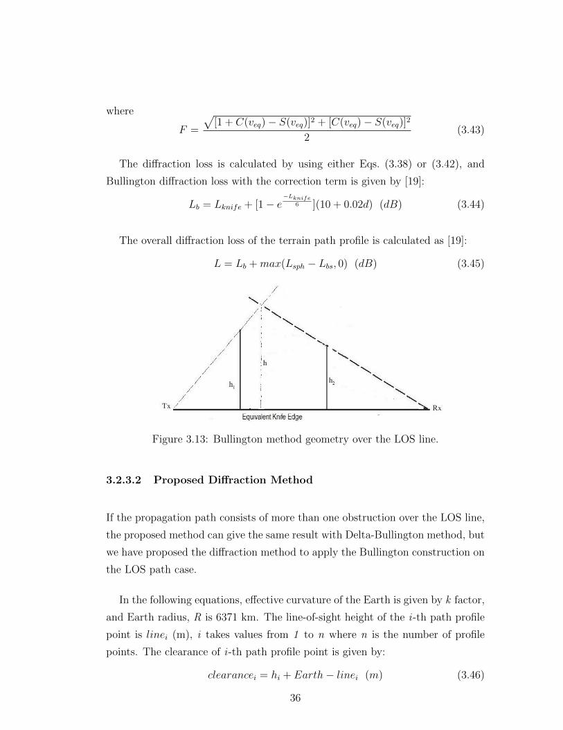
Figure 3.13: Bullington method geometry over the LOS line.

3.2.3.2 Proposed Diffraction Method

If the propagation path consists of more than one obstruction over the LOS line,

the proposed method can give the same result with Delta-Bullington method, but

we have proposed the diffraction method to apply the Bullington construction on

the LOS path case.

In the following equations, effective curvature of the Earth is given by k factor,

and Earth radius, R is 6371 km. The line-of-sight height of the i -th path profile

point is linei (m), i takes values from 1 to n where n is the number of profile

points. The clearance of i -th path profile point is given by:

clearancei = hi + Earth− linei (m) (3.46)

36

Firstly, the dominant profile point with the highest slope of the line from the

transmitter site to the i -th path profile point is determined by using formula of

Eq. (3.47), and the highest slope of the line from the receiver site to the i -th path

profile point is found by using formula of Eq. (3.48).

Stim = max[hi + Earth− htx

di] (mrad) (3.47)

Srim = max[hi + Earth− hrx

d− di] (mrad) (3.48)

where

Earth = 1000× kR[1−cos( d

2kR)

cos∣∣∣ d2−dikR

∣∣∣ ] (m) (3.49)

One hypothetical knife-edge obstacle is defined by the intersection of Stim and

Srim. The distance of an equivalent knife-edge obstacle from the transmitter

site is calculated by using formula of Eq. (3.40). The clearance of an equivalent

knife-edge obstacle is expressed as:

hclearance =

j∑i=1

1

clearancei(3.50)

where j is the number of obstacles along the terrain path profile.

Calculation of the Fresnel diffraction parameter, veq for an equivalent knife-

edge obstacle is given by:

veq = hclearance

√0.002d

λdeq(d− deq)(3.51)

In that case, the diffraction loss of an equivalent knife-edge obstacle is calcu-

lated by using formula of Eq. (3.52). Then, Bullington diffraction loss with the

correction term is calculated by using formula of Eq. (3.44).

Lknife(dB) =

{6.9 + 20log(

√(veq − 0.1)2 + 1 + veq − 0.1) veq > −0.78

−20log(F ) others(3.52)

37

3.3 Diffuse Reflection Loss

In this section, we have described the multipath fading caused by the reflec-

tion points on the terrestrial microwave line-of-sight radio link. The calculation

method of reflection points on the terrain path profile is based on the two-ray

ground reflection model, and the determination of reflection points along the ter-

rain path profile is improved. The procedure for finding reflection points is to

proceed along the path from transmitter site to receiver site, and each path pro-

file point evaluates whether a specular reflection can exist in the profile point in

which the angle of incident from the transmitter is equal to the angle of reflec-

tion to the receiver. The strength of the reflected signal at the receiving antenna

depends on the specular reflection coefficient, the divergence factor due to Earth

curvature, grazing angle, polarization and the directivity of the antennas.

The specular reflection coefficient of the surface, ρ is given by [7]:

ρ =

∣∣∣∣∣sinφ−√C

sinφ+√C

∣∣∣∣∣ (3.53)

where φ is the grazing angle and

C =

{η − cos2φ for horizontal polarization

(η − cos2φ)/η2 for vertical polarization(3.54)

with

η = εr − j18σ

f(3.55)

where εr is the relative permittivity and σ is the conductivity (S/m).

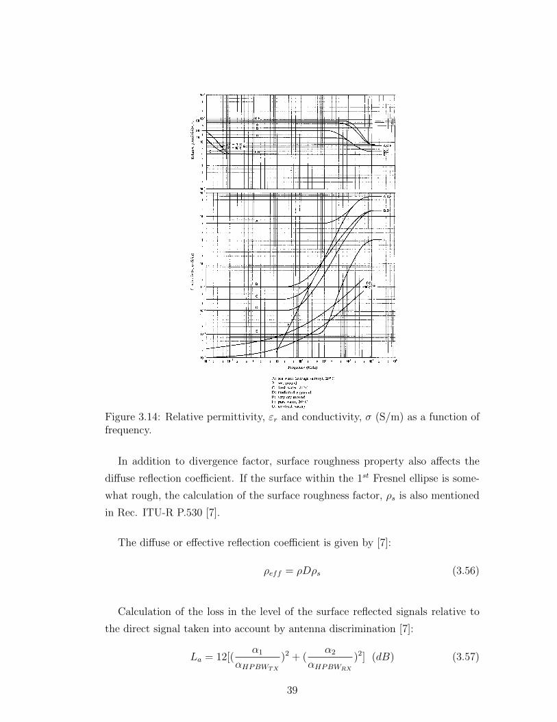
In Fig. 3.14, the values of conductivity and permittivity for different types of

ground as a function frequency are given in Rec. ITU-R P.527 [29].

When an electromagnetic wave is incident on a round path surface, the reflected

wave diverges because of the path surface. So, the energy of the reflected signal

is defocused due to divergence. The calculation of the divergence factor of the

Earth’s surface is mentioned in Rec. ITU-R P.530 [7].

38

D01-sc

Figure 3.14: Relative permittivity, εr and conductivity, σ (S/m) as a function offrequency.

In addition to divergence factor, surface roughness property also affects the

diffuse reflection coefficient. If the surface within the 1st Fresnel ellipse is some-

what rough, the calculation of the surface roughness factor, ρs is also mentioned

in Rec. ITU-R P.530 [7].

The diffuse or effective reflection coefficient is given by [7]:

ρeff = ρDρs (3.56)

Calculation of the loss in the level of the surface reflected signals relative to

the direct signal taken into account by antenna discrimination [7]:

La = 12[(α1

αHPBWTX

)2 + (α2

αHPBWRX

)2] (dB) (3.57)

39

where α1 and α2 are the angles between the direct and reflected waves at trans-

mitter and receiver sites, αHPBWTXand αHPBWRX

are the half-power beamwidth

of the antennas.

The overall loss due to surface reflected wave is given by [7]:

Ls = La − 20log(ρeff ) (dB) (3.58)

If the path profile consists of more than one reflection point on the terrestrial

microwave LOS radio link, the reflection loss of the microwave LOS radio link can

be taken as the minimum of the overall losses due to reflection points, min(Ls).

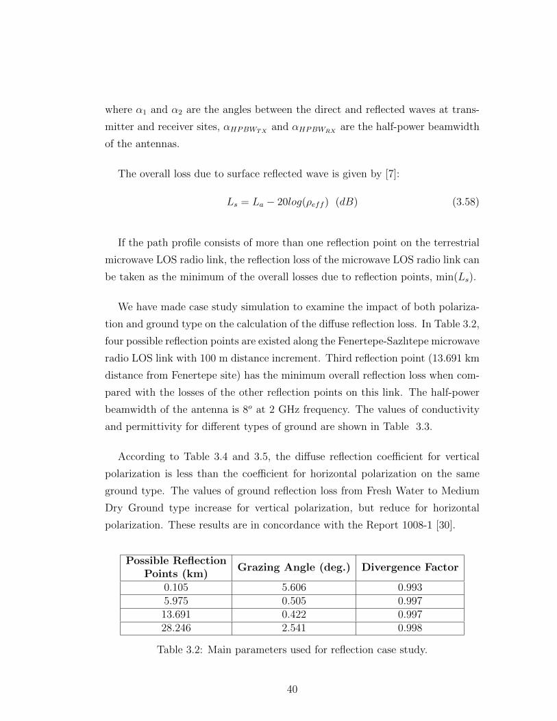
We have made case study simulation to examine the impact of both polariza-

tion and ground type on the calculation of the diffuse reflection loss. In Table 3.2,

four possible reflection points are existed along the Fenertepe-Sazlıtepe microwave

radio LOS link with 100 m distance increment. Third reflection point (13.691 km

distance from Fenertepe site) has the minimum overall reflection loss when com-

pared with the losses of the other reflection points on this link. The half-power

beamwidth of the antenna is 8o at 2 GHz frequency. The values of conductivity

and permittivity for different types of ground are shown in Table 3.3.

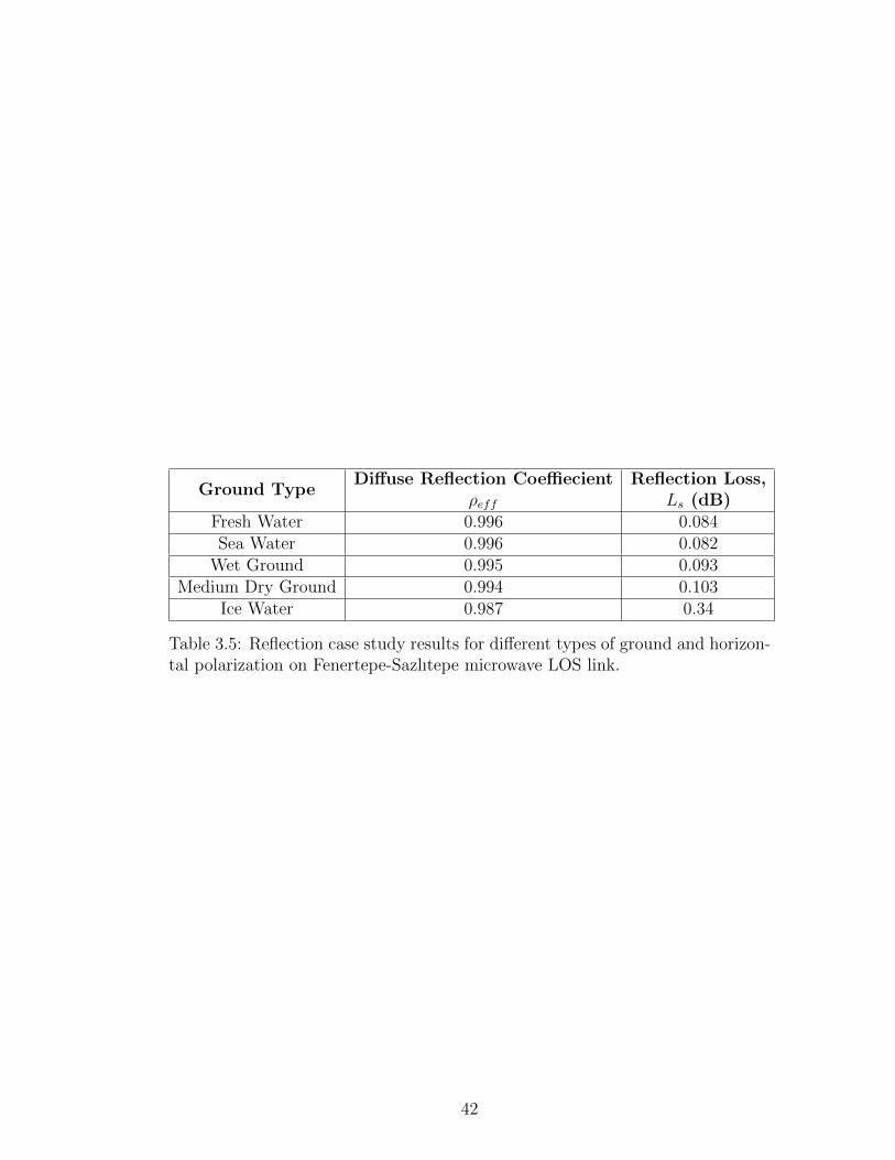
According to Table 3.4 and 3.5, the diffuse reflection coefficient for vertical

polarization is less than the coefficient for horizontal polarization on the same

ground type. The values of ground reflection loss from Fresh Water to Medium

Dry Ground type increase for vertical polarization, but reduce for horizontal

polarization. These results are in concordance with the Report 1008-1 [30].

Possible ReflectionPoints (km)

Grazing Angle (deg.) Divergence Factor

0.105 5.606 0.9935.975 0.505 0.99713.691 0.422 0.99728.246 2.541 0.998

Table 3.2: Main parameters used for reflection case study.

40

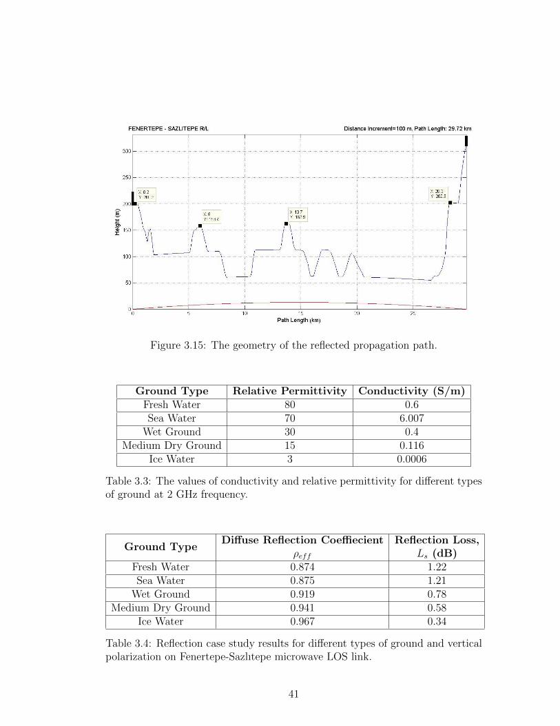
Figure 3.15: The geometry of the reflected propagation path.

Ground Type Relative Permittivity Conductivity (S/m)Fresh Water 80 0.6Sea Water 70 6.007

Wet Ground 30 0.4Medium Dry Ground 15 0.116

Ice Water 3 0.0006

Table 3.3: The values of conductivity and relative permittivity for different typesof ground at 2 GHz frequency.

Ground TypeDiffuse Reflection Coeffiecient

ρeff

Reflection Loss,Ls (dB)

Fresh Water 0.874 1.22Sea Water 0.875 1.21

Wet Ground 0.919 0.78Medium Dry Ground 0.941 0.58

Ice Water 0.967 0.34

Table 3.4: Reflection case study results for different types of ground and verticalpolarization on Fenertepe-Sazlıtepe microwave LOS link.

41

Ground TypeDiffuse Reflection Coeffiecient

ρeff

Reflection Loss,Ls (dB)

Fresh Water 0.996 0.084Sea Water 0.996 0.082

Wet Ground 0.995 0.093Medium Dry Ground 0.994 0.103

Ice Water 0.987 0.34

Table 3.5: Reflection case study results for different types of ground and horizon-tal polarization on Fenertepe-Sazlıtepe microwave LOS link.

42

Chapter 4

LINK ANALYSIS AND

SIMULATION STUDIES

The main propagation effects must be considered in the calculation of the link

availability on the terrestrial microwave LOS/NLOS radio link as shown below:

• Free space loss,

• Attenuation due to atmospheric gases,

• Attenuation due to precipitation,

• Diffraction fading due to obstruction(s) of the path terrain profile,

• Multipath fading due to multipath arising from surface reflection points.

This chapter describes the link budget calculation process, and discusses the

terrain path profile of the terrestrial microwave LOS/NLOS radio link. Examples

of simulation studies are given at the end of this chapter. In a typical microwave

radio link schematic is shown in Fig. 4.1.

43

Figure 4.1: An illustration of a typical microwave radio link.

4.1 Link Power Budget

The prediction of the received signal power is a crucial in the design of fixed

terrestrial microwave LOS/NLOS radio link. A microwave terrestrial microwave

LOS/NLOS radio link designer starts the design process by performing a link

budget analysis. This entails a calculation involving the gains of antennas and

path losses both in clear-air and rainfall conditions as well as noise and interfe-

rence contributions. The path losses here include attenuation due to atmospheric

effects including multipath, diffraction fading due to obstructions of the path

profile, and miscellaneous losses due to couplings at the receiver and transmitter

sites in addition to the free space path loss. The analysis must take into conside-

ration the effective isotropic radiated power, EIRP from the transmitter, and

all the losses just before the receiver. The fade margin calculated from the link

budget calculation is used to determine the link availability under a variety of

fading conditions. At the receiver, the designer needs to also consider receiver

sensitivity. Below the receiver threshold noise level, no signal can be recovered.

Each of the elements in the link budget calculation is discussed below:

44

4.1.1 Free Space Loss

A free space path loss provides a means to predict the received signal power when

there is no object obstructing in the LOS path between the transmitter and the re-

ceiver sites. In line of sight radio systems, losses are mainly due to free space path

loss. As the electromagnetic wave propagates between two geometrically sepa-

rate points, its energy strength reduces with distance even if the path is a clear

of obstacles. In that case of the LOS environment, the received power can fall off

with the square of the distance between the transmitter and the receiver sites. For

this idealistic scenario, the received power is simply given by Friis transmission

equation as [25]:

lFSL =PreceiverPtransmitted

= GTXGRX(λ

4πd)2 (4.1)

where

GTX is the gain of the transmitter antenna in dBi,

GRX is the gain of the receiver antenna in dBi,

λ is wavelength of the transmission in meters,

d is the distance between the transmitter and receiver sites in km.

For simplicity, the basic free space loss assumes unity gain for both transmit-

ting and receiving antennas, and is written as [31]:

LFSL = 92.45 + 20log(d) + 20log(f) (4.2)

where frequency and distance are in GHz and km, respectively.

PaGa multiplication is called EIRP, equivalent isotropically radiated power.

It gives the power radiation at a fixed angle with respect to the isotropic antenna.

But since isotropic antenna is not realistic, sometimes the power is given in terms

of ERP, equivalent radiated power. ERP contains of all gain and loss factors for

both transmitter and receiver sites, and usually expressed in dBm. If Pa is mul-

tiplied with numerical gain with respect to the isotropic antenna, EIRP value is

found. So, gain value of an antenna is given in terms of dBi which is dB gain

of antenna with respect to the isotropic antenna, or dBd which is dB gain of

antenna with respect to the half wave dipole. We can write EIRP= ERP + 2.15

(dBi) since dipole has 2.15 dBi gain.

45

4.1.2 Received Power

The available signal power at the receiver site according to direct signal without

the effect of the ground reflection is expressed by the following relation in dBm:

Pr = TXpower +GTX +GRX−CableLosses− (FSL+Agas+Arain+Adiff ) (4.3)

where

TXpower is the transmitted power in dBm,

GTX is the gain of the transmitting antenna in dBi,

GRX is the gain of the receiving antenna in dBi,

FSL is the free space loss in dB,

Agas is the attenuation due to gases calculated by using formula of Eq. (3.1),

Arain is the attenuation due to rain exceeded for p% of the time on a path of

length in dB calculated by using formula of Eq. (3.8),

Adiff is the diffraction loss in dB.

Multipath fading is an important constraint on the prediction of path loss for

terrestrial line-of-sight microwave links. When the reflected ray reaches the re-

ceiver at the same time as the directed ray, then, they can either add destructively

or constructively resulting in signal attenuation or signal enhancement, respec-

tively. Multipath fading normally gives rise to short-term outages. So, the total

received power with the effect of the ground reflection is given by:

Ptotal = 10 log(10Pr10 × (1− 10

−min(Ls)20 )) (dBm) (4.4)

where Ls are the reflection losses of all reflection points along the terrestrial path

profile in dB.

4.1.3 Noise Power

One of the limitations of the reception quality is noise. The noise power is given

by [11]:

PN = kTeB (4.5)

46

where k is the Boltzmann’s constant= 1.38 × 10−23, Te is the ambient noise

temperature in Kelvin of the environment in which the device operates; it is

usually taken to be 290o, and B is the equivalent bandwith of the link in Hertz.

4.1.4 Coherence Bandwidth

Multipath fading parameters are derived from the total received power. Most

common descriptive parameters are mean excess delay, rms delay spread and

excess delay spread. These parameters are called as time dispersion parameters

due to excess time delays of each different path along the path profile. Mean, τ

and variance, τ 2 excess delay and rms delay spread, στ are given by [25]:

τ =

∑i P (τi)τi∑i P (τi)

(4.6)

τ 2 =

∑i P (τi)τ

2i∑

i P (τi)(4.7)

στ =√τ 2 − (τ)2 (4.8)

Within the coherence bandwidth, Bc all frequency components of the trans-

mitted signal are affected approximately the same, i.e., they undergo the same

attenuation and experience a linear phase shift. For frequency correlation function

above 0.5, coherence bandwidth is given by [25]:

Bc∼=

1

5στ(4.9)

If the propagation path does not have any reflection points along the terrain

path profile, the coherence bandwidth can become infinity.

47

4.1.5 Fade Margin

The fade margin is derived from the link budget calculation, and this parameter

is then used to find the link availability in the terrestrial microwave LOS/NLOS

radio link. Fade margin, also called link margin is a measure of how much margin

is available in the communication link between the functional point and the point

where the link can no longer be available. The fade margin calculation is given

by:

A = Ptotal − PN − SNR (4.10)

where

Ptotal is the received power in dBm calculated by using formula of Eq. (4.4),

PN is the noise power in dBm calculated by using formula of Eq. (4.5),

SNR is target signal-to-noise ratio in dB,

A is the fade margin in dB.

When the fade margin is negative, the signal is received under the specified

bit error rate, or an average worst month outage could occur. The link margin is

related to the link outage probability.

4.1.6 Link Availability

The link availability is the percent of time averaged over a month or a year. The

link availability is calculated by using formula of Eq. (2.5) or (2.8) as a function

of the fade margin. Many fixed microwave radio links are designed to be available

essentially at all times. Usually, link availability of 99.99% for the worst month

is the design goal for fixed links. This implies an outage not exceeding 52.56

minutes in a year. This equivalent link availability level is also referred to by the

shorthand term four nines or 99.99%. The following table summarizes the outage

time per year allowed for given availability percentages.

48

Availability (1-p) Unavailability (p) Outage per year99% 1% 3.65 days

99.9% 0.1% 8.76 hours99.99% 0.01% 52.56 minutes99.999% 0.001% 315.36 seconds

Table 4.1: The outage time per year allowed for given link availability.

4.2 Path Profile and Simulation Studies

A path profile is defined as a geographical representation in two dimensions of

the path followed by the radio beam between the two ends of a radio link. Path

profile helps in determining the elevation height above sea level, and location

of the transmitting and receiving antennas at each of the fixed microwave radio

links. A path profile between transmitter and receiver sites generated using a

Digital Terrain Elevation Data (DTED 1 ) [32] that has a post spacing with 3-arc

seconds or an approximately 100 meters. Once the path profile is drawn, the pre-

ceding information can be used to adjust the terrain path profile for Earth bulge

and k -factor variations. Table A.1 (Appendix A) provides an indication of the

k factor values for different atmospheric refractive conditions. A typical example

of a path profile with k -factor is shown in Fig. A.2.

Fig. 4.2 and 4.3 indicate base station sites for fixed terrestrial microwave

LOS/NLOS radio links studied in both Istanbul and Ankara, Turkey. We applied

simulations on terrestrial microwave LOS/NLOS radio links located in Istanbul

and Ankara, Turkey. Two of these microwave radio links are LOS path case:

Kazan-Elmadag and Fenertepe-Sazlıtepe, respectively. The other microwave ra-

dio links are NLOS or transhorizon path case such as Polatlı-Huseyingazi and

Dikmen-Polatlı, respectively. The main input parameters of these links are sum-

marized in Table 4.2, 4.5, 4.8 and 4.12. The terrain path profiles of the terrestrial

microwave LOS/NLOS radio links are presented in Fig. 2.6, 4.4, 4.5 and 4.6.

49

Figure 4.2: Location of sites used for microwave link simulations in Istanbul.

Figure 4.3: Location of sites used for microwave link simulations in Ankara.

50

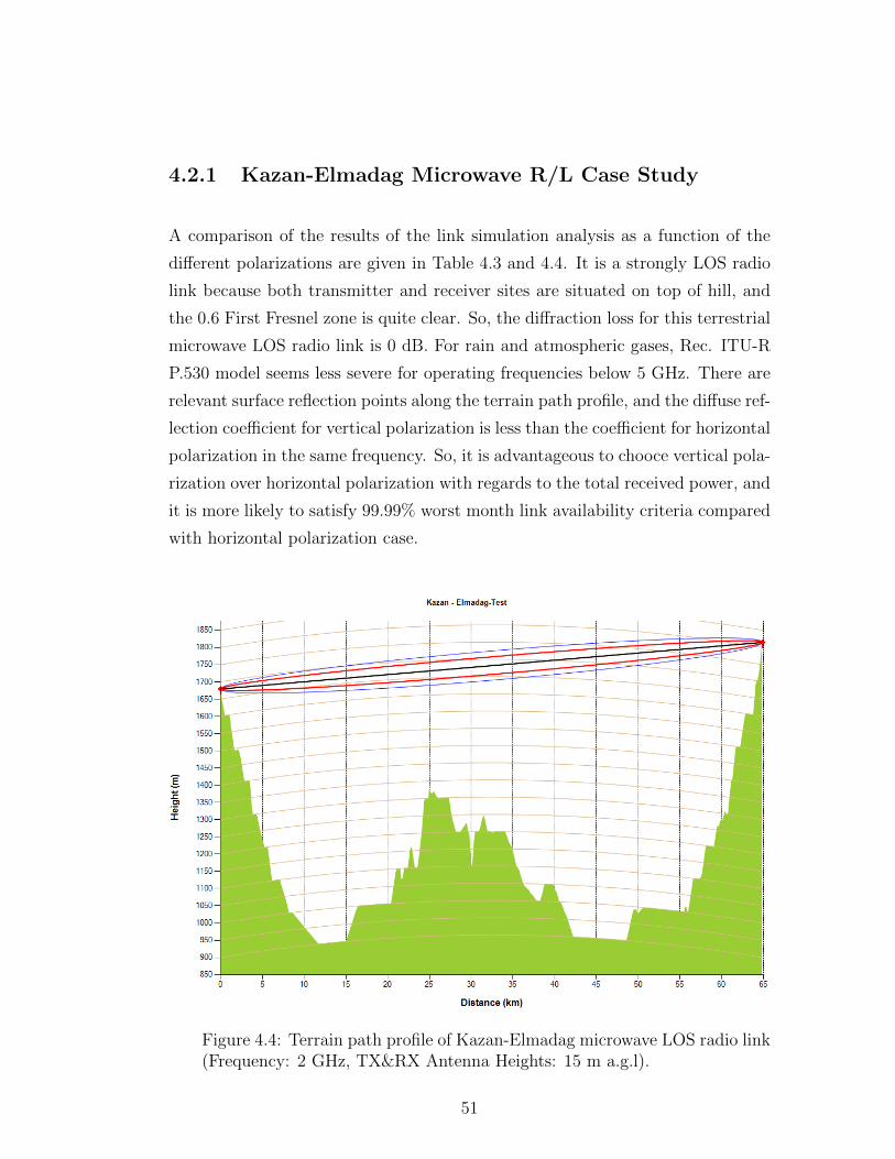
4.2.1 Kazan-Elmadag Microwave R/L Case Study

A comparison of the results of the link simulation analysis as a function of the

different polarizations are given in Table 4.3 and 4.4. It is a strongly LOS radio

link because both transmitter and receiver sites are situated on top of hill, and

the 0.6 First Fresnel zone is quite clear. So, the diffraction loss for this terrestrial

microwave LOS radio link is 0 dB. For rain and atmospheric gases, Rec. ITU-R

P.530 model seems less severe for operating frequencies below 5 GHz. There are

relevant surface reflection points along the terrain path profile, and the diffuse ref-

lection coefficient for vertical polarization is less than the coefficient for horizontal

polarization in the same frequency. So, it is advantageous to chooce vertical pola-

rization over horizontal polarization with regards to the total received power, and

it is more likely to satisfy 99.99% worst month link availability criteria compared

with horizontal polarization case.

Figure 4.4: Terrain path profile of Kazan-Elmadag microwave LOS radio link(Frequency: 2 GHz, TX&RX Antenna Heights: 15 m a.g.l).

51

Parameter Kazan-Elmadag Microwave R/L

Transmitter station, Kazan40o N 18

′37.60”

32o E 36′

43.00”

Receiver station, Elmadag39o N 48

′3.30”

32o E 59′

2.00”

Altitude of transmitter station (a.s.l) 1680 mAltitude of receiver station (a.s.l) 1840 mTX&RX antenna heights (a.g.l) 15 mRadio frequency 1.350, 2 and 2.690 GHzTransmitted power 25 dBmTX&RX antenna gains 22 dBi

HPBW10o for 1.350 GHz

8o for 2 GHz6o for 2.690 GHz

Cablo loss (for each site) 1 dBTarget SNR 6.95 dBBandwith 40 MHzDiffraction method Delta-BullingtonTime percentage for rain attenuation 0.01%Polarization type Vertical and HorizontalGround type Medium Dry GroundSeason type Winter

Table 4.2: Terrestrial link parameters for Kazan-Elmadag microwave LOS radiolink.

52

Parameter Kazan-Elmadag Microwave R/LAzimuth 150.69o

Path inclination 2.475 mradMinimum LOS clearance 61m, 1.00 km from Kazan site

Free space loss131.35 dB for 1.350 GHz134.77 dB for 2.0 GHz

137.34 dB for 2.690 GHz

Attenuation due to atmospheric gases0.37 dB for 1.350 GHz0.40 dB for 2.0 GHz

0.41 dB for 2.690 GHz

Attenuation due to rain0.11 dB for 1.350 GHz0.13 dB for 2.0 GHz

0.18 dB for 2.690 GHzDiffraction loss 0 dB

Attenuation due to reflection loss3.726 dB for 1.350 GHz3.667 dB for 2.0 GHz

3.545 dB for 2.690 GHz

Total received power-68.55 dBm for 1.350 GHz-71.97 dBm for 2.0 GHz

-74.48 dBm for 2.690 GHzNoise power -97.95 dBm

Fade margin22.45 dB for 1.350 GHz19.04 dB for 2.0 GHz

16.52 dB for 2.690 GHz

Link availability99.9976% for 1.350 GHz99.9931% for 2.0 GHz

99.9841% for 2.690 GHz

Table 4.3: Results of link simulation as a function of vertical polarization onKazan-Elmadag terrestrial microwave LOS radio link.

53

Parameter Kazan-Elmadag Microwave R/LAzimuth 150.69o

Path inclination 2.475 mradMinimum LOS clearance 61m, 1.00 km from Kazan site

Free space loss131.35 dB for 1.350 GHz134.77 dB for 2.0 GHz

137.34 dB for 2.690 GHz

Attenuation due to atmospheric gases0.37 dB for 1.350 GHz0.40 dB for 2.0 GHz

0.42 dB for 2.690 GHz

Attenuation due to rain0.09 dB for 1.350 GHz0.13 dB for 2.0 GHz

0.19 dB for 2.690 GHzDiffraction loss 0 dB

Attenuation due to reflection loss5.051 dB for 1.350 GHz

4.956 dB for 2 GHz4.762 dB for 2.690 GHz

Total received power-69.86 dBm for 1.350 GHz-73.25 dBm for 2.0 GHz

-75.71 dBm for 2.690 GHzNoise power -97.95 dBm

Fade margin21.14 dB for 1.350 GHz17.75 dB for 2.0 GHz

15.29 dB for 2.690 GHz

Link availability99.9968% for 1.350 GHz99.9906% for 2.0 GHz

99.9783% for 2.690 GHz

Table 4.4: Results of link simulation as a function of horizontal polarization onKazan-Elmadag terrestrial microwave LOS radio link.

54

4.2.2 Fenertepe-Sazlıtepe Microwave R/L Case Study

Table 4.6 and 4.7 have provided the results of the link simulation analysis in

different polarizations on Fenertepe-Sazlıtepe microwave LOS radio link. It is also

a strongly LOS radio link because the 60% of the first Fresnel zone’s radius is kept

clear, and the diffraction propagation mechanism is negligible in that case. The

analysis of overall performance in terms of the worst month link availability over

the two terrestrial microwave LOS radio links (Kazan-Elmadag and Fenertepe-

Sazlıtepe radio links) shows clearly that these links comply with 99.99% worst

month link availability criteria.

Parameter Fenertepe-Sazlıtepe Microwave R/L

Transmitter station, Fenertepe41o N 09

′2.40”

28o E 47′

9.60”

Receiver station, Sazlıtepe41o N 08

′43.40”

28o E 25′

43.80”

Altitude of transmitter station (a.s.l) 224 mAltitude of receiver station (a.s.l) 340 mAntenna height (a.g.l), Fenertepe 4 mAntenna height (a.g.l), Sazlıtepe 18 mRadio frequency 1.350, 2 and 2.690 GHzTransmitted power 22 dBmTX&RX antenna gains 24 dBi

HPBW10o for 1.350 GHz

8o for 2 GHz6o for 2.690 GHz

Cablo loss (for each site) 1 dBTarget SNR 6.95 dBBandwith 20 MHzDiffraction method Delta-BullingtonTime percentage for rain attenuation 0.01%Polarization type Vertical and HorizontalGround type Medium Dry GroundSeason type Winter

Table 4.5: Terrestrial link parameters for Fenertepe-Sazlıtepe microwave LOSradio link.

55

Parameter Fenertepe-Sazlıtepe Microwave R/LAzimuth 268.95o

Path inclination 4.264 mradMinimum LOS clearance 5m, 0.40 km from Fenertepe site

Free space loss124.57 dB for 1.350 GHz127.98 dB for 2.0 GHz

130.56 dB for 2.690 GHz

Attenuation due to atmospheric gases0.21 dB for 1.350 GHz0.23 dB for 2.0 GHz

0.24 dB for 2.690 GHz

Attenuation due to rain0.09 dB for 1.350 GHz0.23 dB for 2.0 GHz

0.30 dB for 2.690 GHzDiffraction loss 0 dB

Attenuation due to reflection loss5.803 dB for 1.350 GHz

5.7605 dB for 2 GHz5.6691 dB for 2.690 GHz

Total received power-63.08 dBm for 1.350 GHz-66.20 dBm for 2.0 GHz

-68.77 dBm for 2.690 GHzNoise power -100.96 dBm

Fade margin30.94 dB for 1.350 GHz27.81 dB for 2.0 GHz

25.24 dB for 2.690 GHz

Link availability99.9998% for 1.350 GHz99.9971% for 2.0 GHz

99.9934% for 2.690 GHz

Table 4.6: Results of link simulation as a function of vertical polarization onFenertepe-Sazlıtepe terrestrial microwave LOS radio link.

56

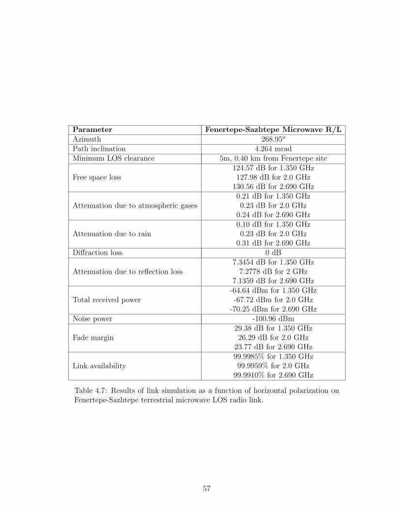
Parameter Fenertepe-Sazlıtepe Microwave R/LAzimuth 268.95o

Path inclination 4.264 mradMinimum LOS clearance 5m, 0.40 km from Fenertepe site

Free space loss124.57 dB for 1.350 GHz127.98 dB for 2.0 GHz

130.56 dB for 2.690 GHz

Attenuation due to atmospheric gases0.21 dB for 1.350 GHz0.23 dB for 2.0 GHz

0.24 dB for 2.690 GHz

Attenuation due to rain0.10 dB for 1.350 GHz0.23 dB for 2.0 GHz

0.31 dB for 2.690 GHzDiffraction loss 0 dB

Attenuation due to reflection loss7.3454 dB for 1.350 GHz

7.2778 dB for 2 GHz7.1359 dB for 2.690 GHz

Total received power-64.64 dBm for 1.350 GHz-67.72 dBm for 2.0 GHz

-70.25 dBm for 2.690 GHzNoise power -100.96 dBm

Fade margin29.38 dB for 1.350 GHz26.29 dB for 2.0 GHz

23.77 dB for 2.690 GHz

Link availability99.9985% for 1.350 GHz99.9959% for 2.0 GHz

99.9910% for 2.690 GHz

Table 4.7: Results of link simulation as a function of horizontal polarization onFenertepe-Sazlıtepe terrestrial microwave LOS radio link.

57

4.2.3 Polatlı-Huseyingazi Microwave R/L Case Study

The path loss predictions are carried out at 1.350, 2.0 and 2.690 GHz frequencies

with a height of 35 m above ground level. It is a NLOS radio link because there is

one obstacle over the LOS line in the first Fresnel ellipsoid. From the Table 4.8,

choice of different diffraction propagation methods plays predominant role in the

calculation of the predicted path loss values on Polatlı-HuseyinGazi microwave

NLOS radio link. As shown in Table 4.10 and 4.11, Delta-Bullington method

overestimates the diffraction loss value due to the correction term, and so it is

less likely to satisfy 99.99% worst month link availability criteria in NATO Band

3+ frequency band. In addition, there are no relevant surface reflection points

along the path profile. So, choice of different polarization types can not affect

the value of the total received power over the terrestrial microwave NLOS radio

link.

Figure 4.5: Terrain path profile of Polatlı-Huseyingazi microwave NLOSradio link (Frequency: 1.35 GHz, TX&RX Antenna Heights: 35 m a.g.l).

58

Parameter Polatlı-Huseyingazi Microwave R/L

Transmitter station, Polatlı39o N 36

′38.00”

32o E 17′

35.00”

Receiver station, Huseyingazi39o N 57

′17.00”

32o E 57′

18.00”

Altitude of transmitter station (a.s.l) 1238 mAltitude of receiver station (a.s.l) 1325 mTX&RX antenna heights (a.g.l) 35 mRadio frequency 1.350, 2 and 2.690 GHzTransmitted power 20 dBmTX&RX antenna gains 27.15 dBi

HPBW10o for 1.350 GHz

8o for 2 GHz6o for 2.690 GHz

Cablo loss (for each site) 3.6 dBTarget SNR 4.95 dBBandwith 20 MHzDiffraction method Delta-Bullington, Epstein-Peterson and DeygoutTime percentage for rain attenuation 0.01%Polarization type Vertical and HorizontalGround type Very Dry GroundSeason type Winter

Table 4.8: Terrestrial link parameters for Polatlı-Huseyingazi microwave NLOSradio link.

59

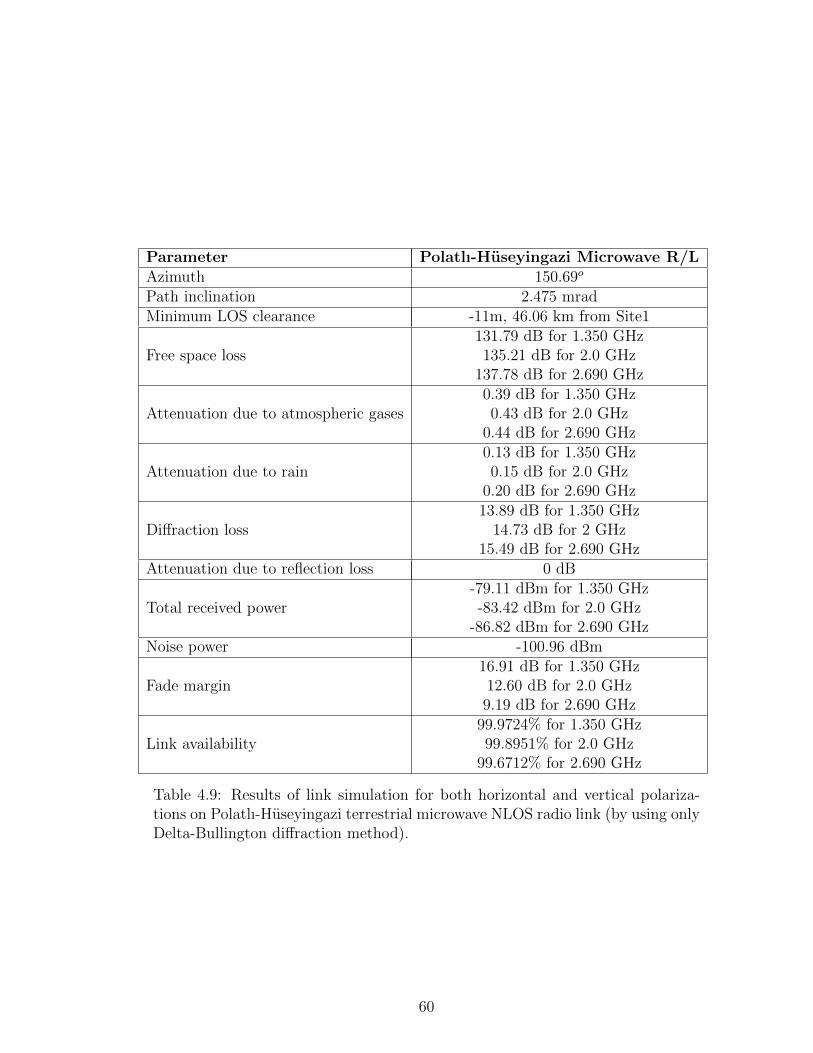
Parameter Polatlı-Huseyingazi Microwave R/LAzimuth 150.69o

Path inclination 2.475 mradMinimum LOS clearance -11m, 46.06 km from Site1

Free space loss131.79 dB for 1.350 GHz135.21 dB for 2.0 GHz

137.78 dB for 2.690 GHz

Attenuation due to atmospheric gases0.39 dB for 1.350 GHz0.43 dB for 2.0 GHz

0.44 dB for 2.690 GHz

Attenuation due to rain0.13 dB for 1.350 GHz0.15 dB for 2.0 GHz

0.20 dB for 2.690 GHz

Diffraction loss13.89 dB for 1.350 GHz

14.73 dB for 2 GHz15.49 dB for 2.690 GHz

Attenuation due to reflection loss 0 dB

Total received power-79.11 dBm for 1.350 GHz-83.42 dBm for 2.0 GHz

-86.82 dBm for 2.690 GHzNoise power -100.96 dBm

Fade margin16.91 dB for 1.350 GHz12.60 dB for 2.0 GHz9.19 dB for 2.690 GHz

Link availability99.9724% for 1.350 GHz99.8951% for 2.0 GHz

99.6712% for 2.690 GHz

Table 4.9: Results of link simulation for both horizontal and vertical polariza-tions on Polatlı-Huseyingazi terrestrial microwave NLOS radio link (by using onlyDelta-Bullington diffraction method).

60

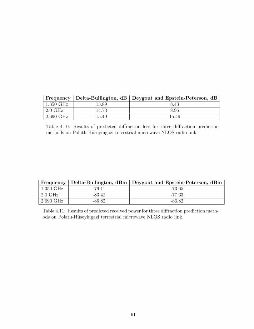
Frequency Delta-Bullington, dB Deygout and Epstein-Peterson, dB1.350 GHz 13.89 8.432.0 GHz 14.73 8.952.690 GHz 15.49 15.49

Table 4.10: Results of predicted diffraction loss for three diffraction predictionmethods on Polatlı-Huseyingazi terrestrial microwave NLOS radio link.

Frequency Delta-Bullington, dBm Deygout and Epstein-Peterson, dBm1.350 GHz -79.11 -73.652.0 GHz -83.42 -77.632.690 GHz -86.82 -86.82

Table 4.11: Results of predicted received power for three diffraction prediction meth-ods on Polatlı-Huseyingazi terrestrial microwave NLOS radio link.

61

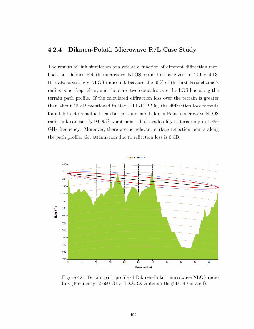
4.2.4 Dikmen-Polatlı Microwave R/L Case Study

The results of link simulation analysis as a function of different diffraction met-

hods on Dikmen-Polatlı microwave NLOS radio link is given in Table 4.13.

It is also a strongly NLOS radio link because the 60% of the first Fresnel zone’s

radius is not kept clear, and there are two obstacles over the LOS line along the

terrain path profile. If the calculated diffraction loss over the terrain is greater

than about 15 dB mentioned in Rec. ITU-R P.530, the diffraction loss formula

for all diffraction methods can be the same, and Dikmen-Polatlı microwave NLOS

radio link can satisfy 99.99% worst month link availability criteria only in 1.350

GHz frequency. Moreover, there are no relevant surface reflection points along

the path profile. So, attenuation due to reflection loss is 0 dB.

Figure 4.6: Terrain path profile of Dikmen-Polatlı microwave NLOS radiolink (Frequency: 2.690 GHz, TX&RX Antenna Heights: 40 m a.g.l).

62

Parameter Dikmen-Polatlı Microwave R/L

Transmitter station, Dikmen39o N 51

′32.00”

32o E 49′

29.00”

Receiver station, Polatlı39o N 36

′38.00”

32o E 17′

35.00”

Altitude of transmitter station (a.s.l) 1339 mAltitude of receiver station (a.s.l) 1243 mTX&RX antenna heights (a.g.l) 40 mRadio frequency 1.350, 2 and 2.690 GHzTransmitted power 30 dBmTX&RX antenna gains 27.15 dBi

HPBW10o for 1.350 GHz

8o for 2 GHz6o for 2.690 GHz

Cablo loss (for each site) 1 dBTarget SNR 4.95 dBBandwith 20 MHzDiffraction method Delta-Bullington, Epstein-Peterson and DeygoutTime percentage for rain attenuation 0.01%Polarization type Vertical and HorizontalGround type Very Dry GroundSeason type Winter

Table 4.12: Terrestrial link parameters for Dikmen-Polatlı microwave NLOS radiolink.

63

Parameter Dikmen-Polatlı Microwave R/LAzimuth 238.90o

Path inclination -1.793 mradMinimum LOS clearance -54m, 29.55 km from Dikmen site

Free space loss129.62 dB for 1.350 GHz133.04 dB for 2.0 GHz

135.61 dB for 2.690 GHz

Attenuation due to atmospheric gases0.30 dB for 1.350 GHz0.33 dB for 2.0 GHz

0.34 dB for 2.690 GHz

Attenuation due to rain0.10 dB for 1.350 GHz0.23 dB for 2.0 GHz

0.25 dB for 2.690 GHz

Diffraction loss (for all diffraction methods)30.09 dB for 1.350 GHz

34.46 dB for 2 GHz38.36 dB for 2.690 GHz

Attenuation due to reflection loss 0 dB

Total received power (for all diffraction methods)-77.82 dBm for 1.350 GHz-85.76 dBm for 2.0 GHz

-92.27 dBm for 2.690 GHzNoise power -100.96 dBm

Fade margin (for all diffraction methods)18.19 dB for 1.350 GHz10.26 dB for 2.0 GHz3.75 dB for 2.690 GHz

Link availability (for all diffraction methods)99.9920% for 1.350 GHz99.9050% for 2.0 GHz

97.6809% for 2.690 GHz

Table 4.13: Results of link simulation for both horizontal and vertical polarizationson Dikmen-Polatlı terrestrial microwave NLOS radio link.

64

Chapter 5

VALIDATION AND

COMPARISON OF RESULTS

In this section, the implementation of link analysis for the design of fixed terres-

trial point-to-point systems is justified by comparison with the commercial ATDI

ICS telecom software [8] and the measurement data existing in the literature [9,10]

over sample fixed terrestrial microwave LOS/NLOS radio links. The short-term

diffraction measurements during August and September 2012 were performed in

the area of Czech Republic with the use of truck-mounted access platform reach-

ing up to 46 meters above ground level mentioned in [9,10] papers. This chapter

is divided into two sections. The first section compares the performance of the

fixed terrestrial microwave LOS radio link in terms of the total received power

with the commercial ATDI ICS telecom software. In the second section, we have

done a comparative case studies between Delta-Bullington diffraction method and

the obtained measurement data [9,10] over the sample fixed terrestrial microwave

LOS/NLOS radio links.

65

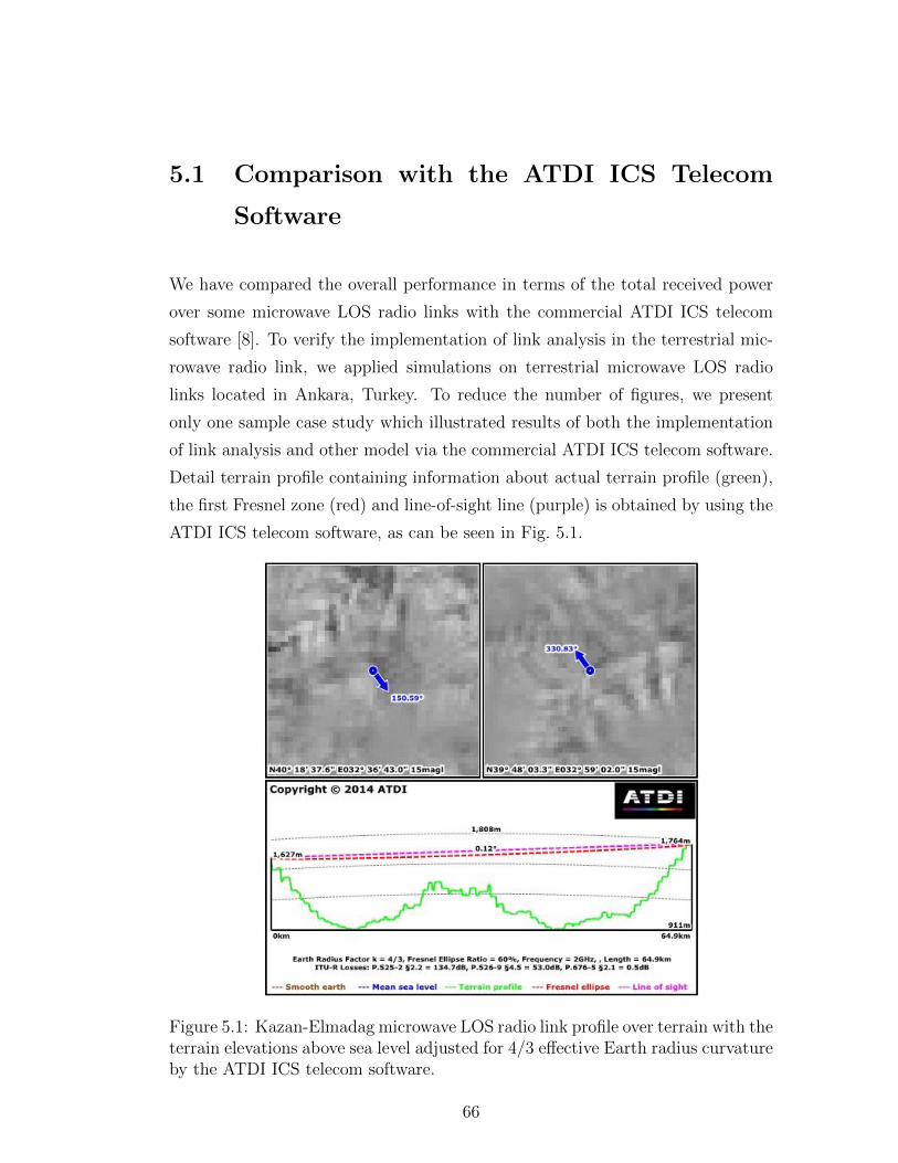
5.1 Comparison with the ATDI ICS Telecom

Software

We have compared the overall performance in terms of the total received power

over some microwave LOS radio links with the commercial ATDI ICS telecom

software [8]. To verify the implementation of link analysis in the terrestrial mic-

rowave radio link, we applied simulations on terrestrial microwave LOS radio

links located in Ankara, Turkey. To reduce the number of figures, we present

only one sample case study which illustrated results of both the implementation

of link analysis and other model via the commercial ATDI ICS telecom software.

Detail terrain profile containing information about actual terrain profile (green),

the first Fresnel zone (red) and line-of-sight line (purple) is obtained by using the

ATDI ICS telecom software, as can be seen in Fig. 5.1.

Figure 5.1: Kazan-Elmadag microwave LOS radio link profile over terrain with theterrain elevations above sea level adjusted for 4/3 effective Earth radius curvatureby the ATDI ICS telecom software.

66

A 64.9 kilometer path from Kazan (N 40o 18′

37.6”, E 32o 36′

43”) to Elmadag

(N 39o 48′

3.3”, E 32o 59′

2”) was selected for the case study as shown in Fig. 5.1.

Kazan antenna height is 1665 m a.s.l, and Elmadag antenna height is 1825 m a.s.l.

The expected rain intensity for 0.01% of the time in this area is 27.66 mm/h.

The link is between Kazan and Elmadag in Turkey with the following link pa-

rameters as shown in Table 5.1. The obtained results are also summarized in

Table 5.2 and 5.3.

The validity of the implementation of link analysis is justified by compari-

son with the commercial ATDI ICS telecom software over sample microwave

LOS/NLOS radio links located in Turkey. The analysis of overall performance in

terms of the total received power over sample microwave LOS radio link shows

that the method is compatible with the other model via ATDI ICS telecom soft-

ware.

Parameter Kazan-Elmadag Microwave R/LAltitude of transmitter station (a.s.l) 1680 mAltitude of receiver station (a.s.l) 1840 mTX&RX antenna heights (a.g.l) 15 mRadio frequency 2 GHzTransmitted power 25 dBmTX&RX antenna gains 22 dBiHPBW 8o

Cablo loss (for each site) 1 dBTarget SNR 6.95 dBBandwith 40 MHzDiffraction method Delta-BullingtonTime percentage for rain attenuation 0.01%Polarization type VerticalGround type Medium Dry GroundSeason type Winter

Table 5.1: Terrestrial link parameters for Kazan-Elmadag terrestrial microwaveLOS radio link (validation case study).

67

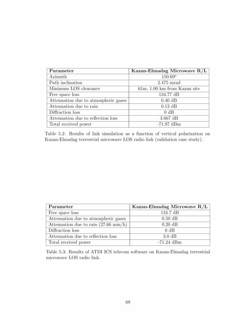
Parameter Kazan-Elmadag Microwave R/LAzimuth 150.69o

Path inclination 2.475 mradMinimum LOS clearance 61m, 1.00 km from Kazan siteFree space loss 134.77 dBAttenuation due to atmospheric gases 0.40 dBAttenuation due to rain 0.13 dBDiffraction loss 0 dBAttenuation due to reflection loss 3.667 dBTotal received power -71.97 dBm

Table 5.2: Results of link simulation as a function of vertical polarization onKazan-Elmadag terrestrial microwave LOS radio link (validation case study).

Parameter Kazan-Elmadag Microwave R/LFree space loss 134.7 dBAttenuation due to atmospheric gases 0.50 dBAttenuation due to rain (27.66 mm/h) 0.20 dBDiffraction loss 0 dBAttenuation due to reflection loss 3.0 dBTotal received power -71.24 dBm

Table 5.3: Results of ATDI ICS telecom software on Kazan-Elmadag terrestrialmicrowave LOS radio link.

68

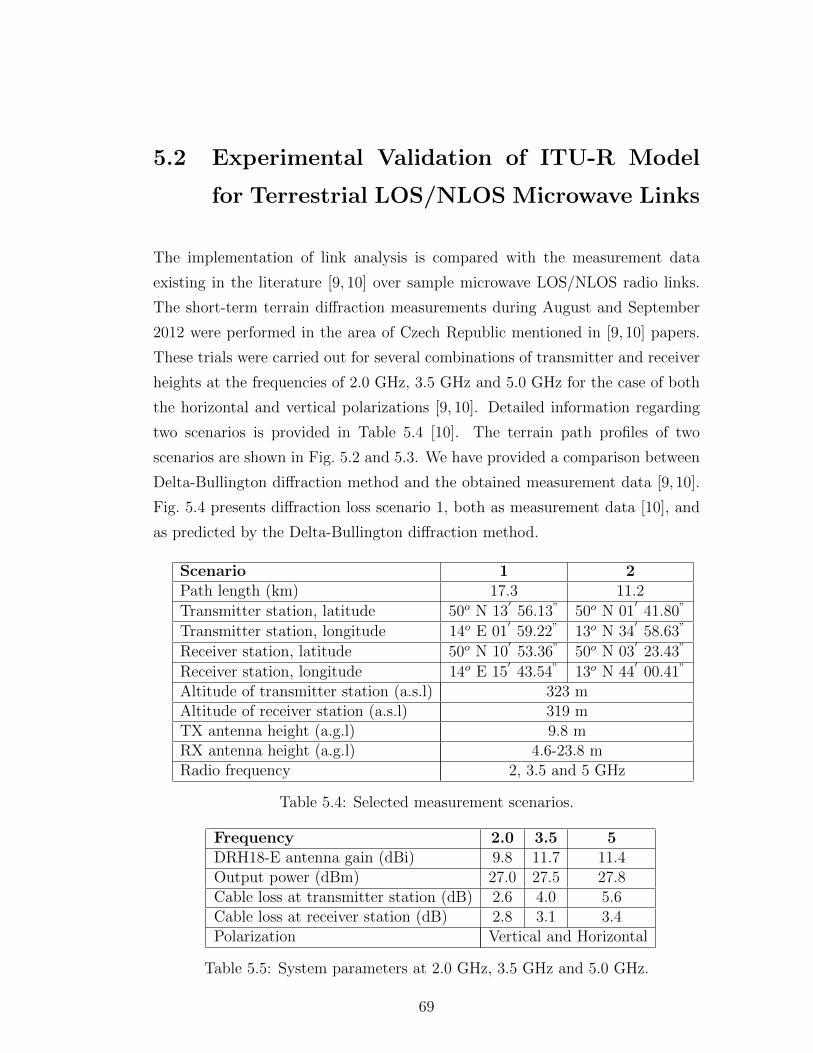
5.2 Experimental Validation of ITU-R Model

for Terrestrial LOS/NLOS Microwave Links

The implementation of link analysis is compared with the measurement data

existing in the literature [9, 10] over sample microwave LOS/NLOS radio links.

The short-term terrain diffraction measurements during August and September

2012 were performed in the area of Czech Republic mentioned in [9, 10] papers.

These trials were carried out for several combinations of transmitter and receiver

heights at the frequencies of 2.0 GHz, 3.5 GHz and 5.0 GHz for the case of both

the horizontal and vertical polarizations [9, 10]. Detailed information regarding

two scenarios is provided in Table 5.4 [10]. The terrain path profiles of two

scenarios are shown in Fig. 5.2 and 5.3. We have provided a comparison between

Delta-Bullington diffraction method and the obtained measurement data [9, 10].

Fig. 5.4 presents diffraction loss scenario 1, both as measurement data [10], and

as predicted by the Delta-Bullington diffraction method.

Scenario 1 2Path length (km) 17.3 11.2

Transmitter station, latitude 50o N 13′

56.13” 50o N 01′

41.80”

Transmitter station, longitude 14o E 01′

59.22” 13o N 34′

58.63”

Receiver station, latitude 50o N 10′

53.36” 50o N 03′

23.43”

Receiver station, longitude 14o E 15′

43.54” 13o N 44′

00.41”

Altitude of transmitter station (a.s.l) 323 mAltitude of receiver station (a.s.l) 319 mTX antenna height (a.g.l) 9.8 mRX antenna height (a.g.l) 4.6-23.8 mRadio frequency 2, 3.5 and 5 GHz

Table 5.4: Selected measurement scenarios.

Frequency 2.0 3.5 5DRH18-E antenna gain (dBi) 9.8 11.7 11.4Output power (dBm) 27.0 27.5 27.8Cable loss at transmitter station (dB) 2.6 4.0 5.6Cable loss at receiver station (dB) 2.8 3.1 3.4Polarization Vertical and Horizontal

Table 5.5: System parameters at 2.0 GHz, 3.5 GHz and 5.0 GHz.

69

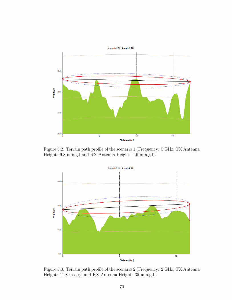
Figure 5.2: Terrain path profile of the scenario 1 (Frequency: 5 GHz, TX AntennaHeight: 9.8 m a.g.l and RX Antenna Height: 4.6 m a.g.l).

Figure 5.3: Terrain path profile of the scenario 2 (Frequency: 2 GHz, TX AntennaHeight: 11.8 m a.g.l and RX Antenna Height: 35 m a.g.l).

70

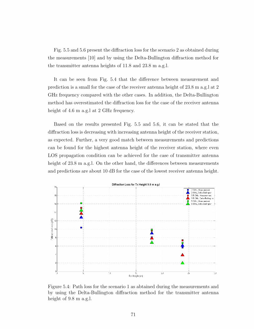
Fig. 5.5 and 5.6 present the diffraction loss for the scenario 2 as obtained during

the measurements [10] and by using the Delta-Bullington diffraction method for

the transmitter antenna heights of 11.8 and 23.8 m a.g.l.

It can be seen from Fig. 5.4 that the difference between measurement and

prediction is a small for the case of the receiver antenna height of 23.8 m a.g.l at 2

GHz frequency compared with the other cases. In addition, the Delta-Bullington

method has overestimated the diffraction loss for the case of the receiver antenna

height of 4.6 m a.g.l at 2 GHz frequency.

Based on the results presented Fig. 5.5 and 5.6, it can be stated that the

diffraction loss is decreasing with increasing antenna height of the receiver station,

as expected. Further, a very good match between measurements and predictions

can be found for the highest antenna height of the receiver station, where even

LOS propagation condition can be achieved for the case of transmitter antenna

height of 23.8 m a.g.l. On the other hand, the differences between measurements

and predictions are about 10 dB for the case of the lowest receiver antenna height.

Figure 5.4: Path loss for the scenario 1 as abtained during the measurements andby using the Delta-Bullington diffraction method for the transmitter antennaheight of 9.8 m a.g.l.

71

Figure 5.5: Path loss for the scenario 2 as abtained during the measurements andby using the Delta-Bullington diffraction method for the transmitter antennaheight of 11.8 m a.g.l.

Figure 5.6: Path loss for the scenario 2 as abtained during the measurements andby using the Delta-Bullington diffraction method for the transmitter antennaheight of 23.8 m a.g.l.

72

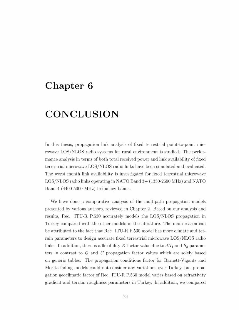
Chapter 6

CONCLUSION

In this thesis, propagation link analysis of fixed terrestrial point-to-point mic-

rowave LOS/NLOS radio systems for rural environment is studied. The perfor-

mance analysis in terms of both total received power and link availability of fixed

terrestrial microwave LOS/NLOS radio links have been simulated and evaluated.

The worst month link availability is investigated for fixed terrestrial microwave

LOS/NLOS radio links operating in NATO Band 3+ (1350-2690 MHz) and NATO

Band 4 (4400-5000 MHz) frequency bands.

We have done a comparative analysis of the multipath propagation models

presented by various authors, reviewed in Chapter 2. Based on our analysis and

results, Rec. ITU-R P.530 accurately models the LOS/NLOS propagation in

Turkey compared with the other models in the literature. The main reason can

be attributed to the fact that Rec. ITU-R P.530 model has more climate and ter-

rain parameters to design accurate fixed terrestrial microwave LOS/NLOS radio

links. In addition, there is a flexibility K factor value due to dN1 and Sa parame-

ters in contrast to Q and C propagation factor values which are solely based

on generic tables. The propagation conditions factor for Barnett-Vigants and

Morita fading models could not consider any variations over Turkey, but propa-

gation geoclimatic factor of Rec. ITU-R P.530 model varies based on refractivity

gradient and terrain roughness parameters in Turkey. In addition, we compared

73

the overall performance of all multipath fading models in terms of total outage

probability over the sample microwave radio link located in Turkey, and so Rec.

ITU-R P.530 model is optimistic.

In Chapter 3, the multipath fading outage prediction method proposed by

Rec. ITU-R P.530 model is studied. All significant clear-air and rainfall propaga-

tion mechanisms are introduced. These propagation mechnanisms are an impor-

tant constraint on the prediction of path losses for fixed terrestrial microwave

LOS/NLOS links at different frequencies. Attenuation due to atmospheric gases

and rain are small for operating frequencies below 5 GHz, and thus often neg-

lected in NATO Band 3+ and NATO Band 4 frequency bands. Diffraction phe-

nomenon occurs when 60% of the first Fresnel zone is obstructed by an obstacle

or several obstacles between the transmitter and receiver sites. The calculation of

the diffraction loss is assuming as a knife-edge. If the propagation path consists

of more than one single knife-edge obstruction, Rec. ITU-R P.526 model suggests

Epstein-Peterson, Deygout and Delta-Bullington methods to calculate the total

diffraction loss due to multiple knife-edges. However, the Epstein-Peterson and

Deygout methods used only for two obstacles over the LOS line. Moreover, if

none of the knife-edges are above the LOS, then Rec. ITU-R P.526 provides the

calculation only on Delta-Bullington method for the diffraction losses. For this

case, Delta-Bullington method is is not based on constructing an equivalent hy-

pothetical single knife-edge at the intersection of transmitter and receiver sites.

Alternatively, we have proposed a multiple knife-edge diffraction method for LOS

line. If the propagation path consists of more than one obstruction over the LOS

line, then our proposed gives the same result with the Delta-Bullington method.

In addition, the calculation of reflection points on the terrain path profile is imp-

roved.

Chapter 4 provides the link budget calculation process in the defined terrestrial

microwave LOS/NLOS radio link. The calculation of both the total received

power with the effect of the ground reflection and the fade margin are developed

to find the link availability in the terrestrial microwave LOS/NLOS radio link. To

complete the microwave performance analysis, we applied simulations on terres-

trial microwave LOS/NLOS radio links located in Istanbul and Ankara, Turkey.

74

According to the link study simulation results, if the terrain path profile is a LOS

radio link, reflection mechanism plays a predominant role on the calculation of

the received power in the terrestrial microwave LOS radio link, and diffraction

fading plays prominent role on the calculation of the received power in another

path profile case. In addition, the implementation of link analysis is compared

by using the ATDI ICS telecom software and the measurement data existing in

the literature over sample fixed terrestrial microwave LOS/NLOS radio links.

The future work will be focused on field measurements which will be used for

better comparison of the results of the link analysis. Data for Turkey should be

collected in the future, to further test and verify the prediction model developed

in this work. Moreover, correlation study and analysis of interference mecha-

nism should be done with the verification of the prediction model. Interference

prediction method proposed by Rec. ITU-R P.452 model [33] will be studied.

75

Appendix A

Effective Earth Radius

The radio refractive index is the ratio of velocity of propagation of a radio wave in

free space to the velocity in a specified medium. At standard atmospheric environ-

ments, the value of the radio refractive index, n has a value of about 1.000312.

Therefore, a more convenient quantity, the atmospheric refractivity N (N-units)

is usually used, and it is given by [21]:

N = (n− 1)× 106 (A.1)

Substituting the value for the ground refractive index (n = 1.000312) into

Eqs. (A.1) yields a N value of 312 N-units. From ITU-R P. 453 [18], N can be

modelled as:

N =77.6

T(P + 4810

e

T) (A.2)

where

P is the total atmospheric pressure in hPa,

e is the water vapour pressure in hPa,

T is the air temperature in degrees.

The value of N varies with altitude since relative humidity, temperature, and

pressure all vary with height. So, pressure and humidity normally decrease

exponentially with height above ground. Humidity and temperature do, how-

ever, change under certain conditions resulting in variations of radio refractivity.

76

In general, the atmosphere displays an exponential decrease of N with height.

For the average atmosphere, refractivity can be written as [18]:

N(h) = Noe− hho (A.3)

where No = 315 N-units for standart atmosphere and for altitudes below 1 km,

ho ∼= 7 km.

The refractivity gradient is defined as:

dN1 =dN

dh(A.4)

From Eq. (A.1), n=(1+N× 10−6) giving

dn

dh=

dN

dh× 10−6 N − units/km (A.5)

and from Eq. (A.3),dN

dh= −No

hoexp(−1/7) (A.6)

For heights less than 1 km, dN/dh is well estimated by its value at 1 km:

dN

dh(1km) = −312

7exp(−1/7) = −38.64 N − units/km (A.7)

When the refractivity gradient displays average characteristics, it is called stan-

dard refraction and corresponds to the commonly quoted value of dN1 = -39 N-

units/km. When it becomes positive, it is known as sub-refraction and can cause

diffraction loss. When the gradient becomes more negative than dN1 = -100 N-

units/km, it is called super-refractive and results in multipath fading. When it

becomes more negative than dN1 = -157 N-units/km, ducting condition occurs

resulting in severe multipath, beam spreading, and even black-out conditions.

These refractivity gradients and their corresponding propagation conditions are

summarized in Table A.1.

The radio ray is imagined to be straight line relative to an effective Earth’s

radius, which has been adjusted by the refractivity gradient. This radius is the

77

real Earth’s radius which has been multiplied by an Earth radius factor k that is

dependent on the refractivity gradient [34]:

k =r

R(A.8)

where

k is the effective Earth radius factor,

r is the effective Earth radius and,

R is the true Earth radius.

The ray curvature for various values of k is shown in Fig. A.1.

Figure A.1: Variation of the ray curvature for different values of k.

The modified radius are found from the relationship [18]:

dn

dh+

1

R=

1

r(A.9)

Common radio links, which are described as LOS, incorrectly propose that

effective communications are restricted by optical horizon (i.e., k = 1). In most

circumstances radio links are not restricted to LOS communication. Communi-

cations further than the optical horizon can often be realized by some 15%( i.e.,

k = 1.33). That is, the k-factor is related to the refractive index gradient by:

k =1

1 +R(dndh

)(A.10)

78

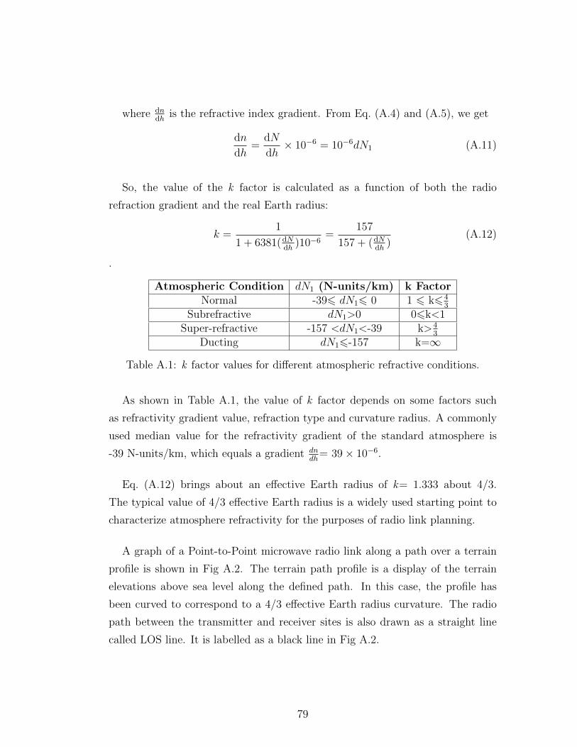
where dndh

is the refractive index gradient. From Eq. (A.4) and (A.5), we get

dn

dh=

dN

dh× 10−6 = 10−6dN1 (A.11)

So, the value of the k factor is calculated as a function of both the radio

refraction gradient and the real Earth radius:

k =1

1 + 6381(dNdh

)10−6=

157

157 + (dNdh

)(A.12)

.

Atmospheric Condition dN1 (N-units/km) k FactorNormal -396 dN16 0 1 6 k64

3

Subrefractive dN1>0 06k<1Super-refractive -157 <dN1<-39 k>4

3

Ducting dN16-157 k=∞

Table A.1: k factor values for different atmospheric refractive conditions.

As shown in Table A.1, the value of k factor depends on some factors such

as refractivity gradient value, refraction type and curvature radius. A commonly

used median value for the refractivity gradient of the standard atmosphere is

-39 N-units/km, which equals a gradient dndh

= 39× 10−6.

Eq. (A.12) brings about an effective Earth radius of k= 1.333 about 4/3.

The typical value of 4/3 effective Earth radius is a widely used starting point to

characterize atmosphere refractivity for the purposes of radio link planning.

A graph of a Point-to-Point microwave radio link along a path over a terrain

profile is shown in Fig A.2. The terrain path profile is a display of the terrain

elevations above sea level along the defined path. In this case, the profile has

been curved to correspond to a 4/3 effective Earth radius curvature. The radio

path between the transmitter and receiver sites is also drawn as a straight line

called LOS line. It is labelled as a black line in Fig A.2.

79

Figure A.2: Polatlı-Elmadag microwave radio link profile over terrain with theterrain elevations above sea level adjusted for 4/3 effective Earth radius curvature.(the blue curve and the red curve indicate the first Fresnel zone and the 0.6 firstFresnel zone, respectively).

80

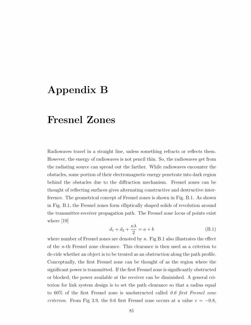
Appendix B

Fresnel Zones

Radiowaves travel in a straight line, unless something refracts or reflects them.

However, the energy of radiowaves is not pencil thin. So, the radiowaves get from

the radiating source can spread out the farther. While radiowaves encounter the

obstacles, some portion of their electromagnetic energy penetrate into dark region

behind the obstacles due to the diffraction mechanism. Fresnel zones can be

thought of reflecting surfaces gives alternating constructive and destructive inter-

ference. The geometrical concept of Fresnel zones is shown in Fig. B.1. As shown

in Fig. B.1, the Fresnel zones form elliptically shaped solids of revolution around

the transmitter-receiver propagation path. The Fresnel zone locus of points exist

where [19]

d1 + d2 +nλ

2= a+ b (B.1)

where number of Fresnel zones are denoted by n. Fig B.1 also illustrates the effect

of the n-th Fresnel zone clearance. This clearance is then used as a criterion to

de-cide whether an object is to be treated as an obstruction along the path profile.

Conceptually, the first Fresnel zone can be thought of as the region where the

significant power is transmitted. If the first Fresnel zone is significantly obstructed

or blocked, the power available at the receiver can be diminished. A general cri-

terion for link system design is to set the path clearance so that a radius equal

to 60% of the first Fresnel zone is unobstructed called 0.6 first Fresnel zone

criterion. From Fig 3.9, the 0.6 first Fresnel zone occurs at a value v = −0.8,

81

which corresponds to the diffraction attenuation of 0.0 dB. In order to calculate

the radius of n-th Fresnel zone, the following conditions should be fulfilled:

4d = (a+ b)− (d1 + d2) =λ

2(B.2)

a =√r21 + d21 => a ≈ d1[1 +

1

2(r1d1

)2 + ...] (B.3)

b =√r21 + d22 => b ≈ d2[1 +

1

2(r1d2

)2 + ...] (B.4)

Taking into account that in practical LOS links, r1 is normally too small in

comparison with d1 and d2, and ignoring the higher order terms of series of the

two last equations, the following equation is given by [19]:

rn ∼=√nλd1d2d1 + d2

(B.5)

where d1(km) is the distance from transmitting antenna to the point where rn

is calculated, d2(km) is the distance from receiving antenna to the point where

rn is calculated, λ in meters is the operating wavelength, and n are Fresnel zone

numbers.

Similarly, the radius of n-th Fresnel zone can be calculated simply by the

following equation [19]:

rn = r1√n (B.6)

As shown in Fig. B.2, an approximate formula [7, 35] for calculating the first

Fresnel zone radius, F1 is given by:

F1 = 17.3

√d1d2

f(d1 + d2)(B.7)

where F1 is the first Fresnel radius in metres, d1 (km) and d2 (km) are the dis-

tances of the obstacles from transmitting and receiving antennas, respectively and

f is the radio frequency in GHz.

82

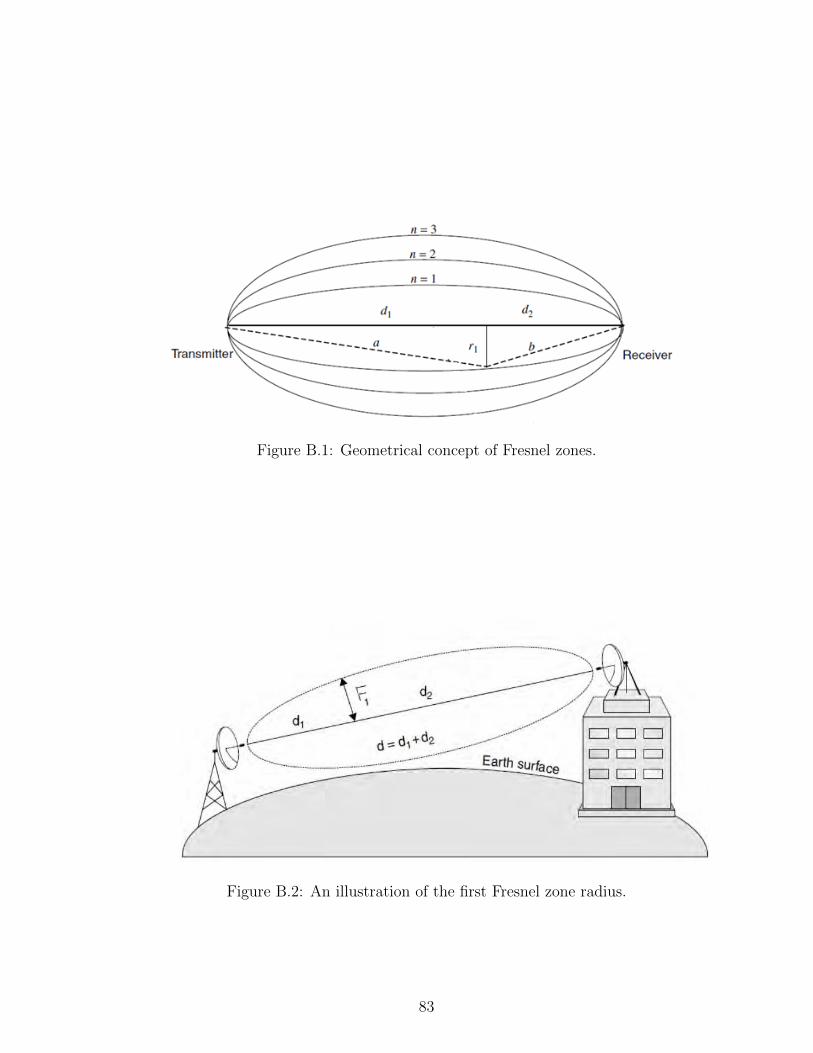
Figure B.1: Geometrical concept of Fresnel zones.

Figure B.2: An illustration of the first Fresnel zone radius.

83

Bibliography

[1] K. Morita, “Prediction of Rayleigh fading occurrence probability of line-

of-sight microwave links,” Rev. Elec. Commun. Lab., vol. 18, pp. 810–821,

Nov.-Dec. 1970.

[2] W. T. Barnett, “Multipath propagation at 4, 6 and 11 GHz,” Bell System

Technical Journal, vol. 51, no. 2, pp. 321–361, February 1972.

[3] A. Vigants, “Space diversity engineering,” Bell System Technical Journal,

vol. 54, no. 1, pp. 103–142, January 1975.

[4] R. L. Olsen and T. Tjelta, “Worldwide techniques for predicting the mul-

tipath fading distribution on terrestrial LOS links: Background and results

of tests,” IEEE Transactions on Antennas and Propagation, vol. 47, no. 1,

pp. 157–170, January 1999.

[5] R. L. Olsen and T. Tjelta, “Worldwide techniques for predicting the multi-

path fading distribution on terrestrial LOS links: Comparison with regional

techniques,” IEEE Transactions on Antennas and Propagation, vol. 51, no. 1,

pp. 23–30, January 2003.

[6] Recommendation ITU-R P.530-8, “Propagation data and prediction meth-

ods required for the design of terrestrial line-of-sight systems,” International

Telecommunication Union, Geneva, 1999.

[7] Recommendation ITU-R P.530-15, “Propagation data and prediction meth-

ods required for the design of terrestrial line-of-sight systems,” International

Telecommunication Union, Geneva, 2013.

84

[8] ATDI ICS telecom software platform. http://www.atdi.com/ics-telecom/.

[9] M. Kvicera, et al., “Short-term terrain diffraction measurements: Pre-

liminary results,” in Proceedings of European Conference on Antenna and

Propagation-7th Eur. Conf. Antennas. Propag., Gothenburg, April 2013, pp.

52-55.

[10] M. Kvicera, et al., “Short-term terrain diffraction measurements from L-

to Q-Band: Results and Analysis,” IEEE Transactions on Antennas and

Propagation, vol. 62, no. 7, pp. 3693–3701, July 2014.

[11] H. R. Anderson, Fixed Broadband Wireless System Design. John Wiley &

Sons Ltd., 2003.

[12] B. L. Agba, et al., “Comparison of microwave links prediction methods:

Barnett-Vigants vs. ITU methods,” in Proceedings of Progress In Electro-

magnetics Research Symposium,, Xi’an, China, March 22-26 2010.

[13] K. T. Vieira, “Comparisons of Barnett-Vigants method with ITU-R link

data base,” tech. rep., EAB/G-03:002609 Uae Ericssonwide Internal Report,

August 2003.

[14] T. Tjelta et al., “Systematic development of new multivariable techniques

for predicting the distribution of multipath fading on terrestrial microwave

links,” IEEE Transactions on Antennas and Propagation, vol. 38, no. 10,

pp. 1650-1665, October 1990.

[15] B. L. Agba, et al., “Recent evolution of ITU method for prediction of mul-

tipath fading on terrestrial microwave links,” in Proceedings of Progress In

Electromagnetics Research Symposium, Marrakesh, Morocco, March 20-23

2011.

[16] D. Sayed, et al., “Comparison between the actual microwave terrestrial links

performance and different models,” in Third International Conference on

Sensor Technologies and Applications,, 2009.

[17] P. Goktas, A. Altintas, S. Topcu and E. Karasan, “The effect of terrain

roughness in the microwave line-of-sight multipath fading estimation based

85

on Rec. ITU-R P.530-15,” in General Assembly and Scientific Symposium

(URSI GASS), 2014 XXXIth URSI, China, August 2014.

[18] Recommendation ITU-R P.453, “The radio refractivity index: its formula

and refractivity data,” International Telecommunication Union, Geneva,

2012.

[19] Recommendation ITU-R P.526, “Propagation by diffraction,” International

Telecommunication Union, Geneva, 2013.

[20] Recommendation ITU-R P.676, “Attenuation by atmospheric gases,” Inter-

national Telecommunication Union, Geneva, 2012.

[21] J. S. Seybold, Introduction to RF Propagation. John Wiley & Sons Ltd.,

2005.

[22] Recommendation ITU-R P.837, “Characteristics of precipitation for propa-

gation modelling,” International Telecommunication Union, Geneva, 2012.

[23] Recommendation ITU-R P.838, “Specific attenuation model for rain for use

in prediction methods,” International Telecommunication Union, Geneva,

2005.

[24] P. Angueira and J. A. Romo, Microwave Line of Sight Link Engineering.

John Wiley & Sons Ltd., 2012.

[25] T. S. Rappaport, Wireless Communications: Principles and Practice (2nd

Edition). ser. Prentice Hall Communications Engineering and Emerging

Technoligies series, Prentice Hall Inc., 2002.

[26] K. Bullington, “Radio propagation at frequencies above 30 Megacycles,” Pro-

ceedings of the Institute of Radio Engineers, vol. 35, pp. 1122-1136, October

1947.

[27] J. Epstein and D. W. Peterson, “An experimental study of wave propaga-

tion at 850 Mc/s,” Proceedings of the Institute of Radio Engineers, vol. 41,

pp. 595-611, May 1953.

86

[28] J. Deygout, “Multiple knife-edge diffraction of microwaves,” IEEE Transac-

tions on Antennas and Propagation, vol. 14, pp. 480-489, July 1966.

[29] Recommendation ITU-R P.527, “Electrical characteristics of the surface of

the Earth,” International Telecommunication Union, Geneva, 1992.

[30] ITU Report 1008-1, “Reflection from the surface of the Earth,” International

Telecommunication Union, Geneva, 1990.

[31] L. Harvey, Microwave Transmission Networks: Planning, Design and Dep-

loyment. McGraw Hill, New York, 2010.

[32] MIL-PRF-89020A, Performance Specification Digital Terrain Elevation

Data, 1996.

[33] Recommendation ITU-R P.452, “Prediction procedure for the evaluation of

interference between stations on the surface of the earth at frequencies above

about 0.1 GHz,” International Telecommunication Union, Geneva, 2013.

[34] T. Manning, Microwave Radio Transmission Design Guide. Artech House,

2009.

[35] R. L. Freeman, Radio System Design for Telecommunications. John Wiley

& Sons Ltd., 1997.

87