analysis and identification of fracture critical members...
TRANSCRIPT

1
Appendix E
Proposed AASHTO Guide Specifications
for
Analysis and Identification of
Fracture Critical Members and
System Redundant Members
2
ATTACHMENT A – 2018 AGENDA ITEM ___ – T-18/T-14
AASHTO Guide Specifications
for
Analysis and Identification of
Fracture Critical Members and
System Redundant Members
3
Foreword Fracture critical members (FCMs) are defined in the AASHTO LRFD Bridge Design Specifications (BDS) (AASHTO, 2017) as steel primary members or portions thereof subject to tension whose failure would probably cause a portion of or the entire bridge to collapse. The decision to define members as FCMs has often been made without considering actual system redundancy or performance of the structure. Prior to the development of the specifications contained herein, no standards existed on how to best perform a system analysis to determine performance and response in the event a FCM is assumed to have failed. NCHRP Project 12-87a was conceived and completed to address all of the important issues related to performing a credible system analysis to identify members in steel bridge structures that should truly be defined as FCMs. Members satisfying the provisions of this Guide Specification may be classified as System Redundant Members (SRMs) as defined in the BDS, and in a FHWA Technical Memorandum dated June 20, 2012 (Lwin, 2012). While the FHWA Memorandum states that system analysis shall only be applied to bridges that are fabricated to the Fracture Control Plan specified in Clause 12 of the AASHTO/AWS D1.5M/D1.5 Bridge Welding Code (AASHTO/AWS, 2015), the provisions contained herein may be applied to any steel bridge that satisfies the specified screening criteria. However, at present, special permission would need to be granted by the FHWA to classify members in such bridges as SRMs. Clearly, the decision to classify members as fracture critical should not be made solely on the basis of the results from 3-D finite-element system analysis. The decision also requires a thorough assessment of the overall fracture vulnerability of the bridge, including details, history, materials, condition, and other factors. Thus, while finite-element analysis (FEA) may demonstrate that a given structure (new or existing) meets the performance criteria contained in these Guide Specifications, any future inspection strategy should depend on an overall assessment of the structure. The assessment would inherently include factors that are difficult to reliably incorporate in a FEA, such as material toughness, presence of fatigue cracks, detailing, residual stresses, age, traffic history, current condition, inspection history, etc. For example, a bridge with members traditionally classified as FCMs that possesses poor details and a history of fatigue cracking probably should not be exempted from in-depth inspection requirements for the entire life of the bridge based solely on system analysis. Alternately, it may be wasteful to perform fracture critical member inspections on a relatively new bridge that is constructed with high quality fabrication using high quality materials, and that is in good condition with details that are designed for infinite life. Thus, the user of this Guide Specification should consider future inspection strategies even when the structure is shown to satisfy the requirements of this Guide Specification. While this Guide Specification does not provide any direction on how to set any sort of future inspection strategies, research by Parr et al. (2010), and Washer et al. (2014) (NCHRP Report 782) provides useful guidance. Throughout this Guide Specification, the condition during which a FCM is assumed to have failed is referred to as the “faulted state”. It is in this condition that these Guide Specifications are intended to apply. These specifications are not applicable to rating or other evaluations when all members are intact. These Guide Specifications provide direction on overall modeling, element selection, and material models suitable for non-linear finite element analysis. Further, two reliability-based load combinations referred to as Redundancy I and Redundancy II have been developed to achieve target reliability indices in the faulted state. These load combinations were developed using the same procedures previously used to create the various load combinations utilized in the current BDS. To determine if the bridge demonstrates sufficient performance in the faulted state, criteria for the strength and service limit states have been developed for comparison to the results of the FEA. The assessment procedures included herein apply to typical steel bridges, such as simple span and continuous I-girder and tub girder bridges, through-girder bridges, truss bridges and tied arch bridges. The Owner’s/Engineer’s discretion may be used to determine other bridge types to which these assessment procedures may or may not apply. It is noted that these assessment procedures were not developed for atypical structures, such as suspension bridges or cable-stayed bridges. It must be taken into account that the specified analysis procedures involve complex non-linear finite-element analysis, which must only be performed by individuals experienced in such finite-element modeling. The commentary directs attention to other documents that provide suggestions for carrying out the requirements and the intent of this Guide Specification. The commentary is not intended to provide every detail as to the development of this Guide Specification, nor is it intended to provide a detailed summary of the studies and research data reviewed in formulating the provisions of this Guide Specification. The reader is encouraged to review the Interim

4
Reports and Final Report for NCHRP Project 12-87a (Connor et al., 2017), which include more complete details and background related to the development of these Guide Specifications.
5
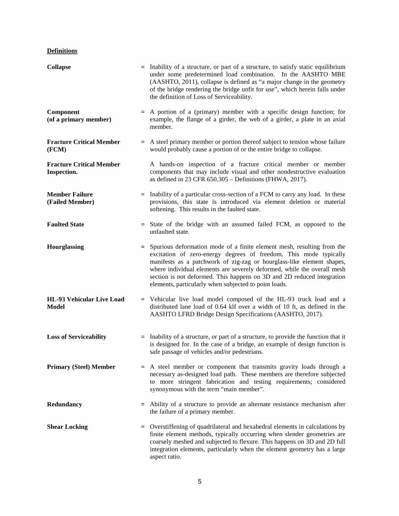
Definitions Collapse = Inability of a structure, or part of a structure, to satisfy static equilibrium
under some predetermined load combination. In the AASHTO MBE (AASHTO, 2011), collapse is defined as “a major change in the geometry of the bridge rendering the bridge unfit for use”, which herein falls under the definition of Loss of Serviceability.
Component (of a primary member)
= A portion of a (primary) member with a specific design function; for example, the flange of a girder, the web of a girder, a plate in an axial member.
Fracture Critical Member (FCM)
= A steel primary member or portion thereof subject to tension whose failure would probably cause a portion of or the entire bridge to collapse.
Fracture Critical Member Inspection.
A hands-on inspection of a fracture critical member or member components that may include visual and other nondestructive evaluation as defined in 23 CFR 650.305 – Definitions (FHWA, 2017).
Member Failure (Failed Member)
= Inability of a particular cross-section of a FCM to carry any load. In these provisions, this state is introduced via element deletion or material softening. This results in the faulted state.
Faulted State = State of the bridge with an assumed failed FCM, as opposed to the unfaulted state.
Hourglassing = Spurious deformation mode of a finite element mesh, resulting from the excitation of zero-energy degrees of freedom. This mode typically manifests as a patchwork of zig-zag or hourglass-like element shapes, where individual elements are severely deformed, while the overall mesh section is not deformed. This happens on 3D and 2D reduced integration elements, particularly when subjected to point loads.
HL-93 Vehicular Live Load Model
= Vehicular live load model composed of the HL-93 truck load and a distributed lane load of 0.64 klf over a width of 10 ft, as defined in the AASHTO LFRD Bridge Design Specifications (AASHTO, 2017).
Loss of Serviceability = Inability of a structure, or part of a structure, to provide the function that it is designed for. In the case of a bridge, an example of design function is safe passage of vehicles and/or pedestrians.
Primary (Steel) Member = A steel member or component that transmits gravity loads through a necessary as-designed load path. These members are therefore subjected to more stringent fabrication and testing requirements; considered synonymous with the term “main member”.
Redundancy = Ability of a structure to provide an alternate resistance mechanism after the failure of a primary member.
Shear Locking = Overstiffening of quadrilateral and hexahedral elements in calculations by finite element methods, typically occurring when slender geometries are coarsely meshed and subjected to flexure. This happens on 3D and 2D full integration elements, particularly when the element geometry has a large aspect ratio.

6
System Redundant Member (SRM)
= A steel primary member or portion thereof subject to tension for which the redundancy is not known by engineering judgment, but which is demonstrated to have redundancy through a refined analysis. SRMs must be designated on the contract documents to be fabricated according to Clause 12 of the AASHTO/AWS D1.5M/D1.5 Bridge Welding Code (AASHTO/AWS, 2015). A SRM need not be subject to the inspection protocols for a FCM as described in 23 CFR 650.305 (FHWA, 2017).
7
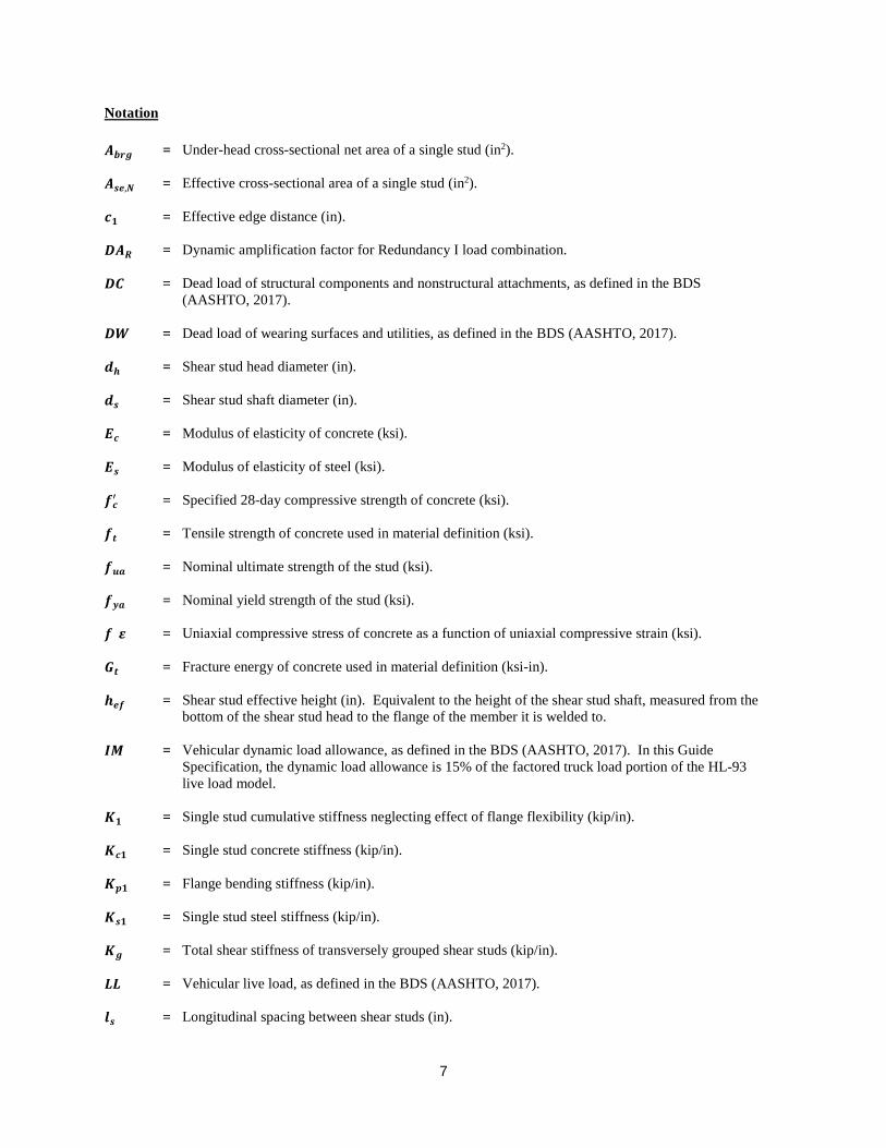
Notation 𝑨𝑨𝒃𝒃𝒃𝒃𝒃𝒃 = Under-head cross-sectional net area of a single stud (in2).
𝑨𝑨𝒔𝒔𝒔𝒔,𝑵𝑵 = Effective cross-sectional area of a single stud (in2).
𝒄𝒄𝟏𝟏 = Effective edge distance (in).
𝑫𝑫𝑨𝑨𝑹𝑹 = Dynamic amplification factor for Redundancy I load combination.
𝑫𝑫𝑫𝑫 = Dead load of structural components and nonstructural attachments, as defined in the BDS
(AASHTO, 2017).
𝑫𝑫𝑫𝑫 = Dead load of wearing surfaces and utilities, as defined in the BDS (AASHTO, 2017).
𝒅𝒅𝒉𝒉 = Shear stud head diameter (in).
𝒅𝒅𝒔𝒔 = Shear stud shaft diameter (in).
𝑬𝑬𝒄𝒄 = Modulus of elasticity of concrete (ksi).
𝑬𝑬𝒔𝒔 = Modulus of elasticity of steel (ksi).
𝒇𝒇𝒄𝒄′ = Specified 28-day compressive strength of concrete (ksi).
𝒇𝒇𝒕𝒕 = Tensile strength of concrete used in material definition (ksi).
𝒇𝒇𝒖𝒖𝒖𝒖 = Nominal ultimate strength of the stud (ksi).
𝒇𝒇𝒚𝒚𝒖𝒖 = Nominal yield strength of the stud (ksi).
𝒇𝒇(𝜺𝜺) = Uniaxial compressive stress of concrete as a function of uniaxial compressive strain (ksi).
𝑮𝑮𝒕𝒕 = Fracture energy of concrete used in material definition (ksi-in).
𝒉𝒉𝒔𝒔𝒇𝒇 = Shear stud effective height (in). Equivalent to the height of the shear stud shaft, measured from the bottom of the shear stud head to the flange of the member it is welded to.
𝑰𝑰𝑰𝑰 = Vehicular dynamic load allowance, as defined in the BDS (AASHTO, 2017). In this Guide Specification, the dynamic load allowance is 15% of the factored truck load portion of the HL-93 live load model.
𝑲𝑲𝟏𝟏 = Single stud cumulative stiffness neglecting effect of flange flexibility (kip/in).
𝑲𝑲𝒄𝒄𝟏𝟏 = Single stud concrete stiffness (kip/in).
𝑲𝑲𝒑𝒑𝟏𝟏 = Flange bending stiffness (kip/in).
𝑲𝑲𝒔𝒔𝟏𝟏 = Single stud steel stiffness (kip/in).
𝑲𝑲𝒃𝒃 = Total shear stiffness of transversely grouped shear studs (kip/in).
𝑳𝑳𝑳𝑳 = Vehicular live load, as defined in the BDS (AASHTO, 2017).
𝒍𝒍𝒔𝒔 = Longitudinal spacing between shear studs (in).
8
𝑵𝑵𝒃𝒃 = Non-modified concrete break-out strength of a single shear stud (kip).
𝑵𝑵𝒄𝒄𝒃𝒃 = Concrete break-out strength of transversely grouped shear studs (kip).
𝑵𝑵𝒃𝒃,𝒏𝒏 = Nominal tensile strength of transversely grouped shear studs (kip).
𝑵𝑵𝒃𝒃(𝜹𝜹𝑵𝑵) = Tension force as a function of axial displacement for a shear stud group embedded in concrete (kip).
𝑵𝑵𝒑𝒑𝒏𝒏 = Pullout strength of transversely grouped shear studs (kip).
𝑵𝑵𝒔𝒔 = Number of transversely grouped shear studs.
𝑵𝑵𝒔𝒔𝒖𝒖 = Tensile rupture strength of transversely grouped shear studs (kip).
𝑵𝑵𝒚𝒚𝒖𝒖 = Tensile yield strength of transversely grouped shear studs (kip).
𝒏𝒏 = Power fit value used in Popovics’ compressive stress-strain relationship for concrete.
𝑸𝑸𝒏𝒏 = Nominal shear resistance of one shear stud embedded in a concrete slab calculated in accordance with LRFD Design Article 6.10.10.4.3 (kip).
𝑸𝑸𝒃𝒃,𝒏𝒏 = Nominal shear resistance of a group of shear studs embedded in a concrete slab (kip).
𝑸𝑸𝒃𝒃(𝜹𝜹𝑸𝑸) = Shear as a function of shear displacement for a shear stud group embedded in concrete (kip).
𝑹𝑹𝒄𝒄 = Shear stud group stiffness coefficient.
𝑺𝑺𝑵𝑵 = Distribution factor for shear stud groups.
𝒔𝒔𝟎𝟎 = Distance from the center of the flange to the outermost stud (in). For a transverse group consisting of one shear stud, 𝒔𝒔𝟎𝟎 shall be taken as zero.
𝒕𝒕𝒇𝒇 = Flange thickness (in).
𝒕𝒕𝒉𝒉 = Net haunch thickness measured from top of top flange to underside of slab (in).
𝒘𝒘𝒄𝒄 = Density of concrete (kcf).
𝒘𝒘𝒉𝒉 = Haunch width (in).
𝜹𝜹𝑵𝑵 = Tensile displacement of a shear stud (in).
𝜹𝜹𝑵𝑵,𝒇𝒇 = Tensile displacement of a shear stud group at failure for shear stud pullout or concrete break-out failure modes (in).
𝜹𝜹𝑸𝑸 = Shear displacement of a shear stud (in).
𝜺𝜺 = Uniaxial compressive strain of concrete.
𝜺𝜺𝒄𝒄 = Compressive strain of concrete at a uniaxial compressive stress equal to 𝑓𝑓𝑐𝑐′.
𝜺𝜺𝒑𝒑𝒍𝒍𝒖𝒖𝒔𝒔𝒕𝒕𝒑𝒑𝒄𝒄 = Plastic strain of concrete.
𝜸𝜸𝑫𝑫𝑫𝑫 = Load factor for structural components and nonstructural attachments.
𝜸𝜸𝑫𝑫𝑫𝑫 = Load factor for wearing surfaces and utilities.

9
𝜸𝜸𝑳𝑳𝑳𝑳 = Load factor for vehicular live load.
𝜸𝜸𝑸𝑸𝒏𝒏 = Total factored load.
𝝍𝝍𝒄𝒄,𝑵𝑵 = Cracking modification factor for calculation of break-out strength of transversely grouped shear
studs.
𝝍𝝍𝒄𝒄,𝑷𝑷 = Cracking modification factor for calculation of pullout strength of transversely grouped shear studs.
𝝍𝝍𝒔𝒔𝒅𝒅,𝑵𝑵 = Edge modification factor for calculation of concrete break-out strength of transversely grouped shear studs.

10
1.0−General
1.1−Scope The provisions contained herein shall be used to evaluate system-level redundancy of a bridge after the failure of a member traditionally designated as a FCM. The results of the evaluation shall place such members into one of two categories: • Fracture Critical Member (FCM) • System Redundant Member (SRM) A FCM may be re-designated as a SRM depending on the outcome of the evaluation using the performance criteria specified in Article 8.0. The primary tension members undergoing evaluation shall be identified on the contract plans as either SRMs or FCMs on new bridges, or as such in the bridge record file for existing bridges. In the case of newly designed yet to be constructed bridges, both FCMs and SRMs shall be fabricated to satisfy the provisions of Clause 12 of the AASHTO/AWS D1.5M/D1.5 Bridge Welding Code. The provisions of Article 9.0 shall also apply. For members which are entirely built-up from components attached using mechanical fasteners, the load-carrying components shall meet the Charpy V-notch toughness (CVN) requirements for those that would traditionally be classified fracture critical tension members specified in AASHTO M 270M/M 270 (ASTM A709/A709M). Unless otherwise specified by the Owner, the assessment procedures included herein shall only be considered applicable to cross girders, and to the following steel-bridge structure types: • Simple-span and continuous-span I-girder (rolled or
fabricated plate sections) and tub-girder bridges (including curved and/or skewed bridges);
• Through-girder bridges; • Truss bridges; and • Tied-arch bridges.
C1.1 The provisions described herein are applicable to existing or newly designed but yet to be constructed steel bridges that are classified as non-redundant and that possess members that are traditionally classified as Fracture Critical Members (FCMs). Traditionally, simple static structural analysis models, experience, and/or engineering judgement have been the typical tools used to identify FCMs. However, it has been shown that steel bridges with members traditionally classified as fracture critical may possess significant reserve strength after the failure of such a member (Connor et al., 2017; Connor et al., 2005; Neuman, 2009; and Cha et al., 2014). These provisions are primarily based on the work reported in NCHRP Project 12-87a (Connor et. al., 2017), in which a finite element methodology was developed to assess whether the failure of a member traditionally classified as fracture critical would result in excessive strain in the remaining members, collapse, or loss of serviceability. The objective of these provisions is to provide guidance on how to best perform a finite-element analysis to evaluate the redundancy of an existing bridge or a bridge under design after the assumed failure of a member traditionally classified as a FCM. Members satisfying these provisions may be classified as System Redundant Members (SRMs) as defined in AASHTO (2017), and in a FHWA Technical Memorandum dated June 20, 2012 (Lwin, 2012). SRMs need not be subject to the inspection protocols for FCMs as described in 23 CFR 650.305 (FHWA, 2017). In the majority of cases, research and in-service performance have demonstrated that conventional bridge designs have provided sufficient redundant capacity after the failure of a member traditionally classified as a FCM. Therefore, while adjustments to a new design may need to be made to satisfy the performance criteria specified herein, these provisions are not intended to be used as the primary basis for the design of a new structure. While the analysis may indicate adequate system redundancy, the special fabrication requirements associated with the provisions of the Fracture Control Plan (FCP) specified in Clause 12 of the AASHTO/AWS D1.5M/D1.5 Bridge Welding Code (AASHTO/AWS, 2015) will decrease the likelihood of future fatigue and fracture issues in the members under evaluation.

11
These provisions are intended to be used in conjunction with other governing AASHTO Specifications, as applicable. The limitations of these provisions are based on the range of structure types and span configurations considered in NCHRP Project 12-87a. Application of these provisions to “atypical” structures, such as suspension bridges or cable-stayed bridges, may require additional research and benchmarking efforts.
1.2−Approach The following steps shall be completed to perform a system analysis: • Perform a Screening according to the provisions
specified in Article 2.
• If the bridge passes the Screening specified in Article 2, perform system modeling as specified in Articles 3 through 8 and illustrated in the flow chart in Figure 1.2-1.
• If the bridge being evaluated is a newly designed
yet to be constructed bridge, the Engineer shall follow the Detailing Requirements for New Bridges specified in Article 9 in the design of the bridge.
C1.2 The Engineer may choose to follow the provisions described in Articles 3 through 8 in a different order than that shown in Figure 1.2-1. However, based on the experience of the authors of this Guide Specification, the process shown in Figure 1.2-1 is usually the most efficient.

12
Figure 1.2-1−Flowchart Describing Finite Element System Analysis Methodology
13
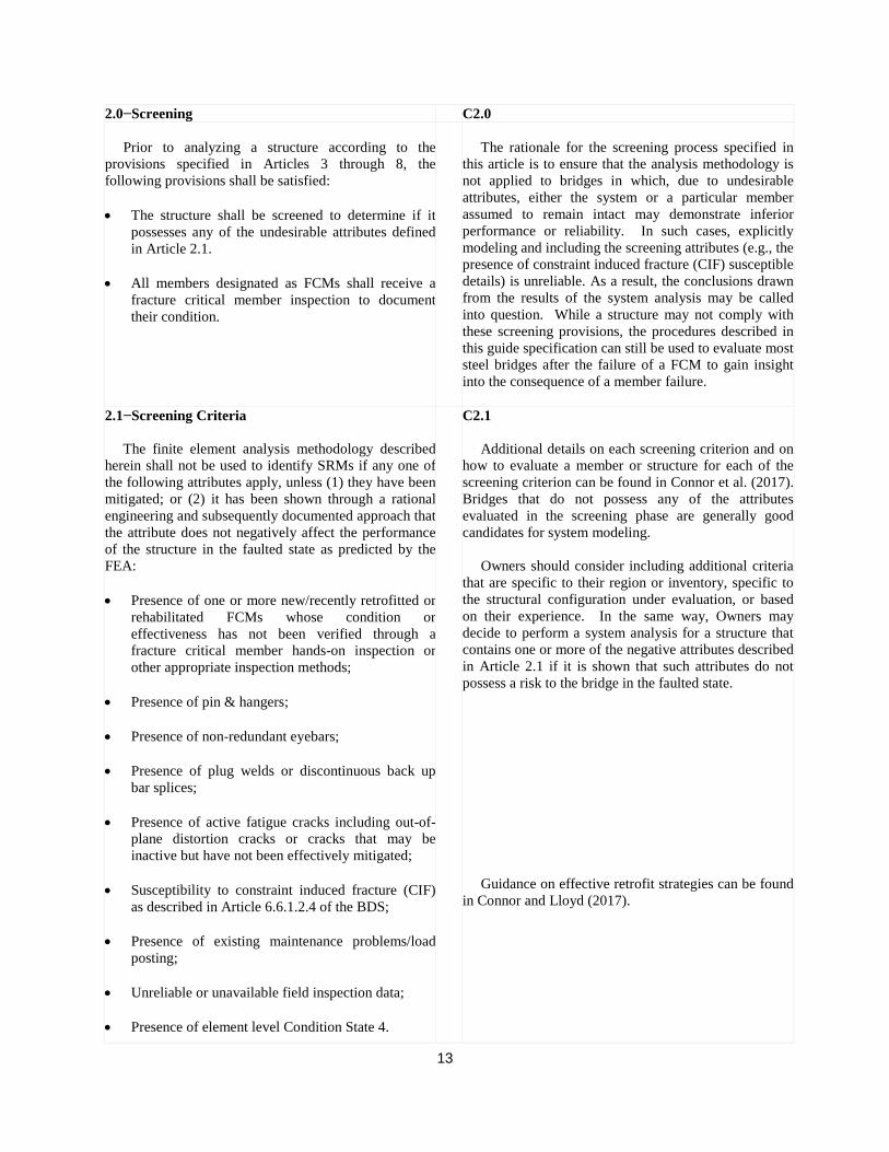
2.0−Screening C2.0 Prior to analyzing a structure according to the provisions specified in Articles 3 through 8, the following provisions shall be satisfied: • The structure shall be screened to determine if it
possesses any of the undesirable attributes defined in Article 2.1.
• All members designated as FCMs shall receive a
fracture critical member inspection to document their condition.
The rationale for the screening process specified in this article is to ensure that the analysis methodology is not applied to bridges in which, due to undesirable attributes, either the system or a particular member assumed to remain intact may demonstrate inferior performance or reliability. In such cases, explicitly modeling and including the screening attributes (e.g., the presence of constraint induced fracture (CIF) susceptible details) is unreliable. As a result, the conclusions drawn from the results of the system analysis may be called into question. While a structure may not comply with these screening provisions, the procedures described in this guide specification can still be used to evaluate most steel bridges after the failure of a FCM to gain insight into the consequence of a member failure.
2.1−Screening Criteria The finite element analysis methodology described herein shall not be used to identify SRMs if any one of the following attributes apply, unless (1) they have been mitigated; or (2) it has been shown through a rational engineering and subsequently documented approach that the attribute does not negatively affect the performance of the structure in the faulted state as predicted by the FEA: • Presence of one or more new/recently retrofitted or
rehabilitated FCMs whose condition or effectiveness has not been verified through a fracture critical member hands-on inspection or other appropriate inspection methods;
• Presence of pin & hangers; • Presence of non-redundant eyebars; • Presence of plug welds or discontinuous back up
bar splices; • Presence of active fatigue cracks including out-of-
plane distortion cracks or cracks that may be inactive but have not been effectively mitigated;
• Susceptibility to constraint induced fracture (CIF)
as described in Article 6.6.1.2.4 of the BDS; • Presence of existing maintenance problems/load
posting; • Unreliable or unavailable field inspection data; • Presence of element level Condition State 4.
C2.1 Additional details on each screening criterion and on how to evaluate a member or structure for each of the screening criterion can be found in Connor et al. (2017). Bridges that do not possess any of the attributes evaluated in the screening phase are generally good candidates for system modeling. Owners should consider including additional criteria that are specific to their region or inventory, specific to the structural configuration under evaluation, or based on their experience. In the same way, Owners may decide to perform a system analysis for a structure that contains one or more of the negative attributes described in Article 2.1 if it is shown that such attributes do not possess a risk to the bridge in the faulted state. Guidance on effective retrofit strategies can be found in Connor and Lloyd (2017).

14
Only the elements that carry load should be considered. For example, a failed coating system does not affect the load carrying capacity in and of itself, although it may lead to accelerated corrosion. The Engineer is advised to evaluate if the presence of element level Condition State 3 for members integral to the system performance in the faulted state compromises the soundness of the redundancy evaluation.
15
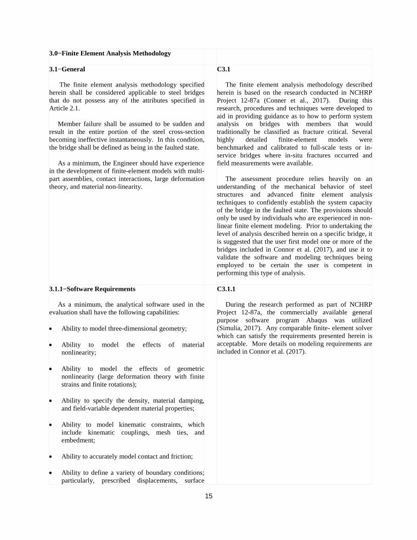
3.0−Finite Element Analysis Methodology
3.1−General The finite element analysis methodology specified herein shall be considered applicable to steel bridges that do not possess any of the attributes specified in Article 2.1. Member failure shall be assumed to be sudden and result in the entire portion of the steel cross-section becoming ineffective instantaneously. In this condition, the bridge shall be defined as being in the faulted state. As a minimum, the Engineer should have experience in the development of finite-element models with multi-part assemblies, contact interactions, large deformation theory, and material non-linearity.
C3.1 The finite element analysis methodology described herein is based on the research conducted in NCHRP Project 12-87a (Conner et al., 2017). During this research, procedures and techniques were developed to aid in providing guidance as to how to perform system analysis on bridges with members that would traditionally be classified as fracture critical. Several highly detailed finite-element models were benchmarked and calibrated to full-scale tests or in-service bridges where in-situ fractures occurred and field measurements were available. The assessment procedure relies heavily on an understanding of the mechanical behavior of steel structures and advanced finite element analysis techniques to confidently establish the system capacity of the bridge in the faulted state. The provisions should only be used by individuals who are experienced in non-linear finite element modeling. Prior to undertaking the level of analysis described herein on a specific bridge, it is suggested that the user first model one or more of the bridges included in Connor et al. (2017), and use it to validate the software and modeling techniques being employed to be certain the user is competent in performing this type of analysis.
3.1.1−Software Requirements As a minimum, the analytical software used in the evaluation shall have the following capabilities: • Ability to model three-dimensional geometry; • Ability to model the effects of material
nonlinearity; • Ability to model the effects of geometric
nonlinearity (large deformation theory with finite strains and finite rotations);
• Ability to specify the density, material damping,
and field-variable dependent material properties; • Ability to model kinematic constraints, which
include kinematic couplings, mesh ties, and embedment;
• Ability to accurately model contact and friction; • Ability to define a variety of boundary conditions;
particularly, prescribed displacements, surface
C3.1.1 During the research performed as part of NCHRP Project 12-87a, the commercially available general purpose software program Abaqus was utilized (Simulia, 2017). Any comparable finite- element solver which can satisfy the requirements presented herein is acceptable. More details on modeling requirements are included in Connor et al. (2017).

16
tractions, and body forces. The software must allow time-dependent input.
3.1.2−Analysis Procedures The analysis procedures shall simulate the following: • Effects of steel dead load; • Effects of dead load from the concrete prior to
curing; • Effects of static or quasi-static loads; • For composite bridges and non-composite bridges,
effects of frictional contact interaction between the girders and slab;
• For composite bridges, effects of the tension and
shear capacities of the shear studs, shear stud pull-out, concrete cracking, and the transverse and longitudinal shear stud spacing;
• Effects of static or quasi-static member failure.
C3.1.2 It is generally acceptable to assume all concrete is placed at once and is uniformly cured. Shrinkage effects should be neglected. Inertial effects due to the dynamic response of the bridge due to the member failure are accounted for in the Redundancy I load combination specified in Article 3.4. The analysis should be performed so that inertial effects due to the application of loads are minimized.
3.1.3−Minimum FCM/SRM Failure Scenarios The failure scenarios to be considered shall be those which produce the greatest demands on the remaining intact components. The locations of the failure scenarios shall be selected based on the criticality of the member failure to the response of the system in the faulted state, and may not necessarily be coincident with any specific detail. The approach for introducing the failure of a primary steel tension member shall be contingent upon the selected approach for estimating the dynamic amplification following the sudden failure of the member as specified in Article 3.3. The bridge or component shall be evaluated under the loading combinations specified in Article 3.4. As a minimum, the following basic individual failure scenarios shall be considered. Other scenarios shall be evaluated as deemed necessary. Both strength and serviceability checks shall be made for each scenario as specified in Article 8.0. Only one member shall be assumed to have failed at any instant in time in any one scenario. Multiple failure scenarios may need to be considered for a particular bridge at the discretion of the Owner or the Engineer. The entire cross-section of the member shall be assumed
C3.1.3 This article provides minimum failure scenarios for evaluation when conducting the system analysis. It is important to recognize that the objective of the analysis is to evaluate the consequence of a member failure that is assumed to have occurred at the worst location. While the most likely location could be at a poor fatigue detail on an existing bridge for example, failure at such a location may not result in the worst-case scenario. While it is not possible to address every conceivable failure scenario in these provisions, the Engineer should consider those scenarios which are plausible and likely to result in the greatest demands on the remaining intact components. In many cases or in complex structures, other member failure scenarios in addition to those specified herein should be considered since it may not be readily apparent which scenario results in the most critical outcome. The scenarios to be considered should be agreed upon between the Owner and the Engineer.
17
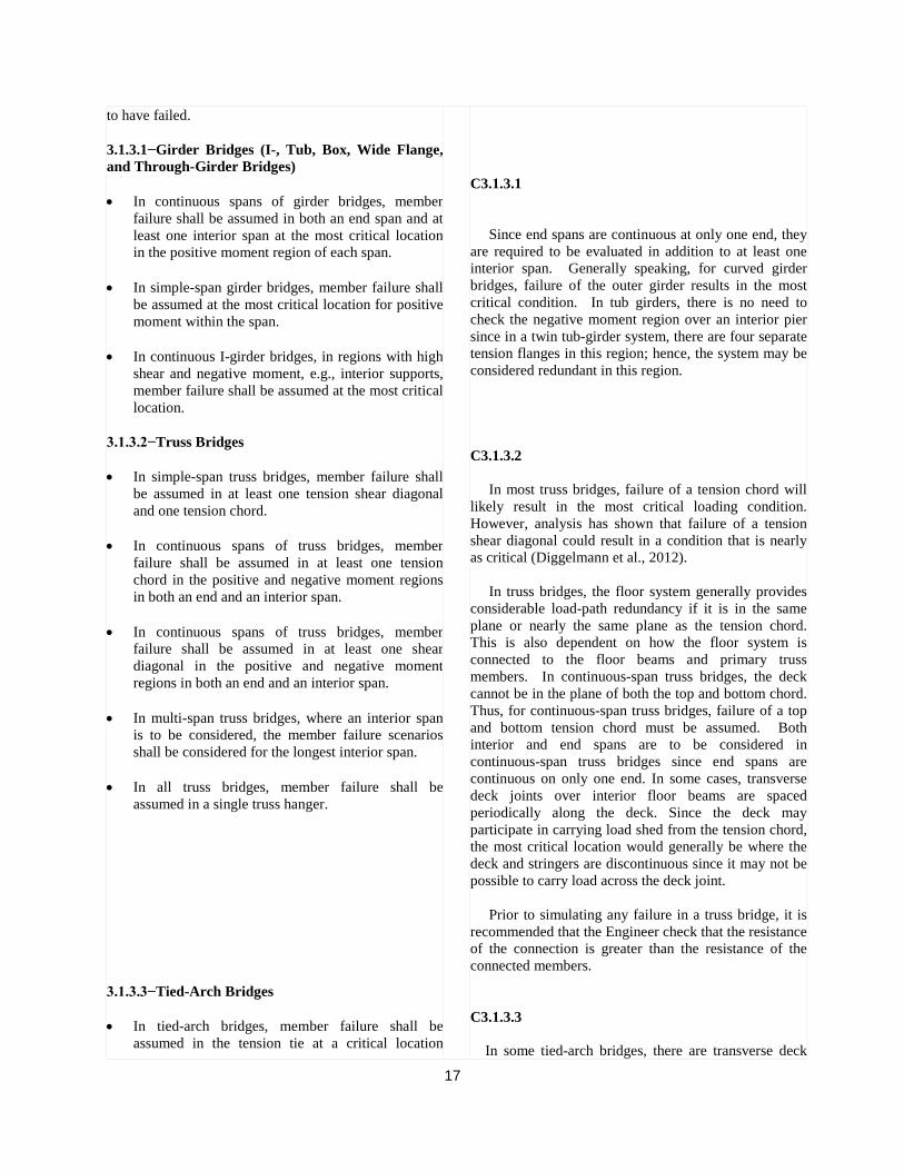
to have failed. 3.1.3.1−Girder Bridges (I-, Tub, Box, Wide Flange, and Through-Girder Bridges) • In continuous spans of girder bridges, member
failure shall be assumed in both an end span and at least one interior span at the most critical location in the positive moment region of each span.
• In simple-span girder bridges, member failure shall
be assumed at the most critical location for positive moment within the span.
• In continuous I-girder bridges, in regions with high
shear and negative moment, e.g., interior supports, member failure shall be assumed at the most critical location.
3.1.3.2−Truss Bridges • In simple-span truss bridges, member failure shall
be assumed in at least one tension shear diagonal and one tension chord.
• In continuous spans of truss bridges, member
failure shall be assumed in at least one tension chord in the positive and negative moment regions in both an end and an interior span.
• In continuous spans of truss bridges, member
failure shall be assumed in at least one shear diagonal in the positive and negative moment regions in both an end and an interior span.
• In multi-span truss bridges, where an interior span
is to be considered, the member failure scenarios shall be considered for the longest interior span.
• In all truss bridges, member failure shall be
assumed in a single truss hanger. 3.1.3.3−Tied-Arch Bridges • In tied-arch bridges, member failure shall be
assumed in the tension tie at a critical location
C3.1.3.1 Since end spans are continuous at only one end, they are required to be evaluated in addition to at least one interior span. Generally speaking, for curved girder bridges, failure of the outer girder results in the most critical condition. In tub girders, there is no need to check the negative moment region over an interior pier since in a twin tub-girder system, there are four separate tension flanges in this region; hence, the system may be considered redundant in this region. C3.1.3.2 In most truss bridges, failure of a tension chord will likely result in the most critical loading condition. However, analysis has shown that failure of a tension shear diagonal could result in a condition that is nearly as critical (Diggelmann et al., 2012). In truss bridges, the floor system generally provides considerable load-path redundancy if it is in the same plane or nearly the same plane as the tension chord. This is also dependent on how the floor system is connected to the floor beams and primary truss members. In continuous-span truss bridges, the deck cannot be in the plane of both the top and bottom chord. Thus, for continuous-span truss bridges, failure of a top and bottom tension chord must be assumed. Both interior and end spans are to be considered in continuous-span truss bridges since end spans are continuous on only one end. In some cases, transverse deck joints over interior floor beams are spaced periodically along the deck. Since the deck may participate in carrying load shed from the tension chord, the most critical location would generally be where the deck and stringers are discontinuous since it may not be possible to carry load across the deck joint. Prior to simulating any failure in a truss bridge, it is recommended that the Engineer check that the resistance of the connection is greater than the resistance of the connected members. C3.1.3.3 In some tied-arch bridges, there are transverse deck

18
within the span. This location may be at mid-span or at a location where the deck and stringers are discontinuous, such as at a deck joint at some location near mid-span.
• In tied-arch bridges, member failure shall be
assumed in the tension tie near the intersection with the arch.
3.1.3.4−Floor Beams • In a single interior floor beam, member failure shall
be assumed at mid-span of the floor beam. Floor beams located where stringers are not continuous and/or where deck joints are present shall be investigated.
3.1.3.5−Cross Girders • In cross girders, member failure shall be assumed at
midpan and near the support or column.
joints over interior floor beams that are spaced periodically along the deck. Since the deck may participate in carrying load shed from the tie girder, the most critical location would likely be where the deck and stringers are discontinuous since it may not be possible to carry load across the deck joint. C3.1.3.5 Cross girders are often referred to by other names, such as integral pier caps or transverse steel bent caps, etc. Regardless, these provisions are applicable to any transverse element fabricated from steel that supports the superstructure.
3.2−Loads
3.2.1−Dead Load Dead load shall consist of all gravity loads and shall be applied to the structure as body forces. Future dead loads that may be detrimental to the performance of the structure in the faulted state should be considered.
C3.2.1 In cases where future dead loads will likely be applied, such as a future wearing surface, these loads should be considered in the evaluation.
3.2.2−Live Load The applied live load shall consist of the HL-93 vehicular live load model as defined in LRFD Design Article 3.6.1.2. The application of live load shall depend on the orientation of the member that is assumed to have failed. In the evaluation of truss bridges, verticals, diagonals, and chords shall be treated as longitudinal members.
C3.2.2 The vehicular live load specified in this article is considered to be a minimum. The Engineer may need to consider additional live load scenarios. The specific application of the HL-93 vehicular live load model is different for the Redundancy I load combination than for the Redundancy II load combination. These load combinations are specified in Article 3.4.
3.2.2.1−Longitudinal Primary Members C3.2.2.1 For longitudinal primary members, the number of lanes that are to be considered in the redundancy evaluation shall be taken as follows: • For the Redundancy I load combination, only the
striped or normal travel lane(s) shall be considered. • For the Redundancy II load combination, the
19
number of lanes to be considered shall be taken as specified in LRFD Design Article 3.6.1.1.1.
The transverse positioning of live load for the redundancy evaluation of longitudinal primary members shall be as follows: • For the Redundancy I load combination, the design
truck or design tandem and the 10.0-ft loaded width of the HL-93 vehicular live load model shall be centered within the striped or normal travel lane(s).
• For the Redundancy II load combination, the design
lanes shall be positioned transversely to produce the largest demands on the remaining intact components of the bridge. The HL-93 live load model shall be transversely place within the design lanes to produce the largest demands on the remaining components of the structure. The design truck or design tandem shall be positioned transversely such that the center of any wheel load is not closer than 2.0 ft from the edge of the design lane.
The longitudinal positioning of live load for the redundancy evaluation of longitudinal primary members shall be as follows: • Where the failure section is in a region of positive
moment under dead load, the centroid of the design truck or design tandem of the HL-93 vehicular live load model shall be positioned longitudinally coincident with the location of the assumed damage in the faulted member.
• When the failure section is in a region of negative
moment under dead load, the HL-93 vehicular live load model shall be applied as described in the third bullet of LRFD Design Article 3.6.1.3.1.
While vehicles may occasionally be positioned outside of the normal travel lanes, i.e., striped lanes, it was deemed to be overly conservative to position vehicles outside of the normal travel lanes for the Redundancy I load combination, which is considered to be an instantaneous point-in-time load combination.
3.2.2.2−Transverse Members For transverse members such as floor beams, live load shall be positioned as specified in Article 3.2.2.1. However, live load shall only be applied within the region of the deck between the next adjacent floor beam or transverse member.
3.3−Dynamic Amplification Following Sudden Member Failure Dynamic amplification immediately following the sudden failure of a tension member when evaluating the Redundancy I load combination specified in Article 3.4
C3.3 The dynamic amplification referred to in this article is that which is produced immediately following the sudden failure of a tension member as the result of the free vibration of the structure, which occurs as the
20
shall be estimated according to one of the approaches specified in Articles 3.3.1 and 3.3.2.
structure reaches a new position of equilibrium. It is not related to the typical dynamic load allowance, e.g., IM, which is intended to account for the effects of trucks traveling across the bridge at highway speeds. These approaches are not intended to capture the effects of the high-velocity stress waves that may propagate throughout the structure in the event of a sudden brittle fracture. Testing has shown that there is no need to model this stress wave propagation (Diggelmann et al., 2012; Neuman, 2009; Hebdon et al., 2015; and Goto et al., 2011).
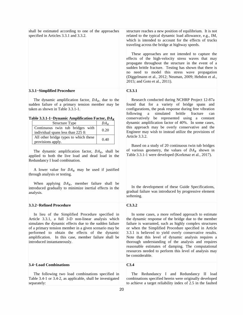
3.3.1−Simplified Procedure The dynamic amplification factor, 𝐷𝐷𝐷𝐷𝑅𝑅, due to the sudden failure of a primary tension member may be taken as shown in Table 3.3.1-1. Table 3.3.1-1−Dynamic Amplification Factor, 𝑫𝑫𝑨𝑨𝑹𝑹
Structure Type 𝐷𝐷𝐷𝐷𝑅𝑅 Continuous twin tub bridges with individual spans less than 225 ft 0.20
All other bridge types to which these provisions apply. 0.40
The dynamic amplification factor, 𝐷𝐷𝐷𝐷𝑅𝑅, shall be applied to both the live load and dead load in the Redundancy I load combination. A lower value for 𝐷𝐷𝐷𝐷𝑅𝑅 may be used if justified through analysis or testing. When applying 𝐷𝐷𝐷𝐷𝑅𝑅, member failure shall be introduced gradually to minimize inertial effects in the analysis.
C3.3.1 Research conducted during NCHRP Project 12-87a found that for a variety of bridge spans and configurations, the peak response during free vibration following a simulated brittle fracture can conservatively be represented using a constant dynamic amplification factor of 40%. In some cases, this approach may be overly conservative and the Engineer may wish to instead utilize the provisions of Article 3.3.2. Based on a study of 20 continuous twin tub bridges of various geometry, the values of 𝐷𝐷𝐷𝐷𝑅𝑅 shown in Table 3.3.1-1 were developed (Korkmaz et al., 2017). In the development of these Guide Specifications, gradual failure was introduced by progressive element softening.
3.3.2−Refined Procedure In lieu of the Simplified Procedure specified in Article 3.3.1, a full 3-D non-linear analysis which simulates the dynamic effects due to the sudden failure of a primary tension member in a given scenario may be performed to obtain the effects of the dynamic amplification. In this case, member failure shall be introduced instantaneously.
C3.3.2 In some cases, a more refined approach to estimate the dynamic response of the bridge due to the member failure is warranted, such as highly complex structures or when the Simplified Procedure specified in Article 3.3.1 is believed to yield overly conservative results. Note that this level of dynamic analysis requires a thorough understanding of the analysis and requires reasonable estimates of damping. The computational resources needed to perform this level of analysis may be considerable.
3.4−Load Combinations The following two load combinations specified in Table 3.4-1 or 3.4-2, as applicable, shall be investigated separately:
C3.4 The Redundancy I and Redundancy II load combinations specified herein were originally developed to achieve a target reliability index of 2.5 in the faulted

21
• Redundancy I - Load combination relating to dead
load and a point-in-time live load applied at the instant when the assumed failure of the member occurs. This load combination is intended to capture the effects of dynamic amplification during free vibration immediately following the member failure in the presence of dead load and live load.
• Redundancy II – Load combination relating to the
normal vehicular use of the bridge without wind after the failure of a primary member. This load combination is intended to characterize the loading scenario after the assumed fracture has occurred and the structure has reached a steady state.
state. During the development of the load factors for these load combinations, it was recognized that for bridges designed and fabricated to meet the AASHTO/AWS FCP, brittle fracture has been shown to be a highly remote possibility. In fact, since the introduction of the FCP over 40 years ago, there have not been any such failures observed on bridges built to the FCP. Hence, a lower target reliability index of 1.5 was selected for bridges fabricated and built to the FCP to reflect this excellent service record. Use of the apparent lower load factors specified in Table 3.4-1 has been deemed appropriate in the load model since it is recognized that the actual risk associated with a fracture is much lower due to the remote possibility of fracture in bridges fabricated to the AASHTO/AWS FCP. Hence, the actual failure rate of these structures is much lower than implied by the chosen target reliability index of 1.5. The Redundancy I load combination represents the applied loading at the instant in time at which the assumed member failure occurs. In order to include the effects of free vibration of the structure following sudden failure of a tension member, all loads are to be amplified by the dynamic amplification factor, 𝐷𝐷𝐷𝐷𝑅𝑅, specified in Article 3.3.1, unless the Refined Procedure specified in Article 3.3.2 is utilized to simulate these effects. The Redundancy II load combination represents the live load that may be expected and that the bridge must withstand after the assumed fracture has occurred, but before it has been detected. In many cases, the damage will be detected quickly, such as in ramp structures in busy urban areas. However, in other cases, such as structures in remote areas and where the resulting dead load deflection is small, it is recognized that it may be some time before the fracture is detected; hence, the need for the Redundancy II load combination. Experience has shown that for typical multi-span twin tub girder bridges with unfactored dead load to live load ratios less than about 2.0 and a 𝐷𝐷𝐷𝐷𝑅𝑅 of 0.20, the Redundancy II load combination will most likely control in continuous-span girder bridges.
For each of the above load combinations, the total factored load, 𝛾𝛾𝑄𝑄𝑛𝑛, to be applied shall be calculated using the following equation:
𝛾𝛾𝑄𝑄𝑛𝑛 = (1 + 𝐷𝐷𝐷𝐷𝑅𝑅)[𝛾𝛾𝐷𝐷𝐷𝐷𝐷𝐷𝐷𝐷 + 𝛾𝛾𝐷𝐷𝐷𝐷𝐷𝐷𝐷𝐷+ 𝛾𝛾𝐿𝐿𝐿𝐿(𝐿𝐿𝐿𝐿 + 𝐼𝐼𝐼𝐼)] (3.4-1)
The structural reliability principles utilized in the calibration of the BDS, which are described in NCHRP Report 368 (Nowak, 1999), were utilized in the calculation of the load factors for the Redundancy I and Redundancy II load combinations. The calculation procedure is based on the algorithm developed by Rackwitz and Fiessler (1977).
22
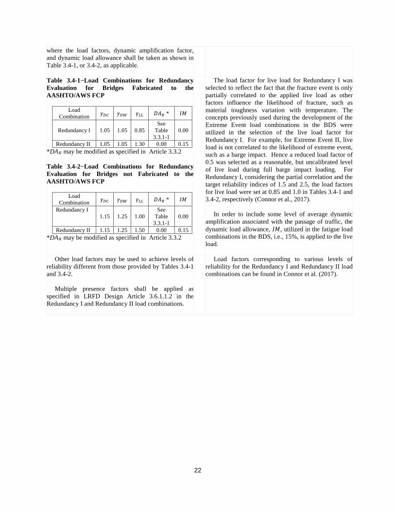
where the load factors, dynamic amplification factor, and dynamic load allowance shall be taken as shown in Table 3.4-1, or 3.4-2, as applicable.
Table 3.4-1−Load Combinations for Redundancy Evaluation for Bridges Fabricated to the AASHTO/AWS FCP
Load Combination 𝛾𝛾𝐷𝐷𝐷𝐷 𝛾𝛾𝐷𝐷𝐷𝐷 𝛾𝛾𝐿𝐿𝐿𝐿 𝐷𝐷𝐷𝐷𝑅𝑅 * 𝐼𝐼𝐼𝐼
Redundancy I 1.05 1.05 0.85 See
Table 3.3.1-1
0.00
Redundancy II 1.05 1.05 1.30 0.00 0.15 *DAR may be modified as specified in Article 3.3.2 Table 3.4-2−Load Combinations for Redundancy Evaluation for Bridges not Fabricated to the AASHTO/AWS FCP
Load Combination 𝛾𝛾𝐷𝐷𝐷𝐷 𝛾𝛾𝐷𝐷𝐷𝐷 𝛾𝛾𝐿𝐿𝐿𝐿 𝐷𝐷𝐷𝐷𝑅𝑅 * 𝐼𝐼𝐼𝐼
Redundancy I 1.15 1.25 1.00
See Table
3.3.1-1 0.00
Redundancy II 1.15 1.25 1.50 0.00 0.15 *DAR may be modified as specified in Article 3.3.2
The load factor for live load for Redundancy I was selected to reflect the fact that the fracture event is only partially correlated to the applied live load as other factors influence the likelihood of fracture, such as material toughness variation with temperature. The concepts previously used during the development of the Extreme Event load combinations in the BDS were utilized in the selection of the live load factor for Redundancy I. For example, for Extreme Event II, live load is not correlated to the likelihood of extreme event, such as a barge impact. Hence a reduced load factor of 0.5 was selected as a reasonable, but uncalibrated level of live load during full barge impact loading. For Redundancy I, considering the partial correlation and the target reliability indices of 1.5 and 2.5, the load factors for live load were set at 0.85 and 1.0 in Tables 3.4-1 and 3.4-2, respectively (Connor et al., 2017). In order to include some level of average dynamic amplification associated with the passage of traffic, the dynamic load allowance, 𝐼𝐼𝐼𝐼, utilized in the fatigue load combinations in the BDS, i.e., 15%, is applied to the live load.
Other load factors may be used to achieve levels of reliability different from those provided by Tables 3.4-1 and 3.4-2. Multiple presence factors shall be applied as specified in LRFD Design Article 3.6.1.1.2 in the Redundancy I and Redundancy II load combinations.
Load factors corresponding to various levels of reliability for the Redundancy I and Redundancy II load combinations can be found in Connor et al. (2017).

23
4.0 Material Models 4.1−Structural Steel and Reinforcing Steel The following material model shall be assumed for structural steel and reinforcing steel: • Steel elastic modulus, 𝐸𝐸𝑠𝑠, equal to 29,000 ksi; • Poisson’s ratio equal to 0.3; • Onset of plasticity is assumed to take place at the
nominal yield strength and the material hardens until the nominal ultimate strength is reached. The hardening is linear and kinematic as shown in Figure 4.1-1;
• The failure strain may be assumed at the minimum
specified elongation at failure, with a permitted maximum strain of 0.05.
Modifications to the specified steel material model may be permitted if substantiated by data from material testing.
Figure 4.1-1–Assumed Steel Stress-Strain Curve
C4.1 Inelastic response of steel is best described by Von Mises (J2) plasticity with a combination of kinematic and isotropic hardening. Most steels are better described by purely kinematic hardening than purely isotropic hardening, especially at the beginning of the inelastic portion of the material response. However, the use of isotropic or kinematic hardening only plays a role when the structure is subjected to plastic strain reversal. Instead of using failure strains related to uniaxial tension tests, the failure strain may be conservatively assumed to be 0.05. This may seem conservative compared to strains observed in tension-test specimens with smooth machined surfaces. However, real connections and structures include welded connections, drilled holes for connections, thermally cut edges, or other features of a typical fabricated member which may result in a loss of ductility. Hence, the 0.05 limit on strain is specified. Further, the material may be subjected to a biaxial state of stress. It is recognized that machined tensile-test specimens will demonstrate higher levels of strain prior to failure. Once the failure strain is attained the element is assumed to fail. Less restrictive values of the fracture strain, i.e., greater than 0.05, may be used by the Engineer during a specific evaluation if they have been substantiated by testing or other documented literature.
4.2−Reinforced Concrete In the absence of available material test data, the empirical models described in Articles 4.2.1 and 4.2.2 shall be used to define the compressive behavior and tensile behavior, respectively, of reinforced concrete. The material constitutive model for concrete shall be concrete damage plasticity. The interaction between the concrete and reinforcing steel shall be included as described in Article 5.2. Perfect bonding may be assumed by embedding the reinforcing steel in the concrete.
C4.2 Concrete damage plasticity assumes that the main two failure mechanisms are tensile cracking and compressive crushing of the concrete material. The evolution of the yield (or failure) surface is controlled by two hardening variables, tensile and compressive equivalent plastic strains, linked to failure mechanisms under tension and compression loading, respectively (Lubliner et al., 1989 and Lee & Fenves, 1998).

24
4.2.1−Concrete Compressive Behavior The following features of the concrete compressive behavior shall be considered: the concrete elastic modulus, 𝐸𝐸𝑐𝑐; concrete 28-day compressive strength, 𝑓𝑓𝑐𝑐′; dilation; confinement; non-associated flow; and compressive crushing. Initially, the material shall be assumed to be linearly elastic with Poisson’s ratio equal to 0.2 and elastic modulus, 𝐸𝐸𝑐𝑐, as follows:
where:
The relation between concrete compressive stress, 𝑓𝑓(𝜀𝜀), and compressive strain, 𝜀𝜀, in the inelastic range shall be taken as follows:
where:
The power fit value used in Popovics’ compressive stress-strain relationship for concrete, 𝑛𝑛, shall be taken as follows:
The compressive strain of concrete at a uniaxial compressive stress equal to 𝑓𝑓𝑐𝑐′, 𝜀𝜀𝑐𝑐, shall be taken as follows:
𝐸𝐸𝑐𝑐 = 33,000(𝑤𝑤𝑐𝑐)1.5(𝑓𝑓𝑐𝑐′)0.5 ≤ 1802.5(𝑓𝑓𝑐𝑐′)0.5
(4.2.1-1)
𝑓𝑓𝑐𝑐′ = specified 28-day compressive strength of concrete (ksi)
𝑤𝑤𝑐𝑐 = density of concrete (kcf)
𝑓𝑓(𝜀𝜀) = 𝑓𝑓𝑐𝑐′ �𝜀𝜀𝜀𝜀𝑐𝑐� �
𝑛𝑛
�𝑛𝑛 − 1 + � 𝜀𝜀𝜀𝜀𝑐𝑐�𝑛𝑛��
(4.2.1-2)
𝑛𝑛 = power fit value used in Popovics’
compressive stress-strain relationship for concrete
𝜀𝜀 = uniaxial compressive strain of concrete 𝜀𝜀𝑐𝑐 = compressive strain of concrete at a uniaxial
compressive stress equal to 𝑓𝑓𝑐𝑐′
𝑛𝑛 = 0.4𝑓𝑓𝑐𝑐, + 1.0 (4.2.1-3)
𝜀𝜀𝑐𝑐 = 0.00124(𝑓𝑓𝑐𝑐′)0.25 (4.2.1-4)
C4.2.1 Under uniaxial compression, the response should be linear until the value of initial yield. In the plastic regime, the response is typically characterized by stress hardening followed by strain softening beyond the ultimate stress. The proposed compressive stress-strain relation is based on the empirical curve proposed by Popovics (1973) to define concrete uniaxial behavior. Popovics’ stress-strain relation is entirely defined by the compressive strength and two constants; one related to the cementitious material type, i.e., concrete, mortar or paste; and another related to the type of aggregate and test method used. This relation was compared against a comprehensive set of experimental test resulting in good correlation as reported by Popovics (1973). The typical compression stress-strain curve of the Popovics’ model is shown in Figure C4.2.1.
Figure C4.2.1–Assumed Concrete Compression Stress-Strain Curve
25
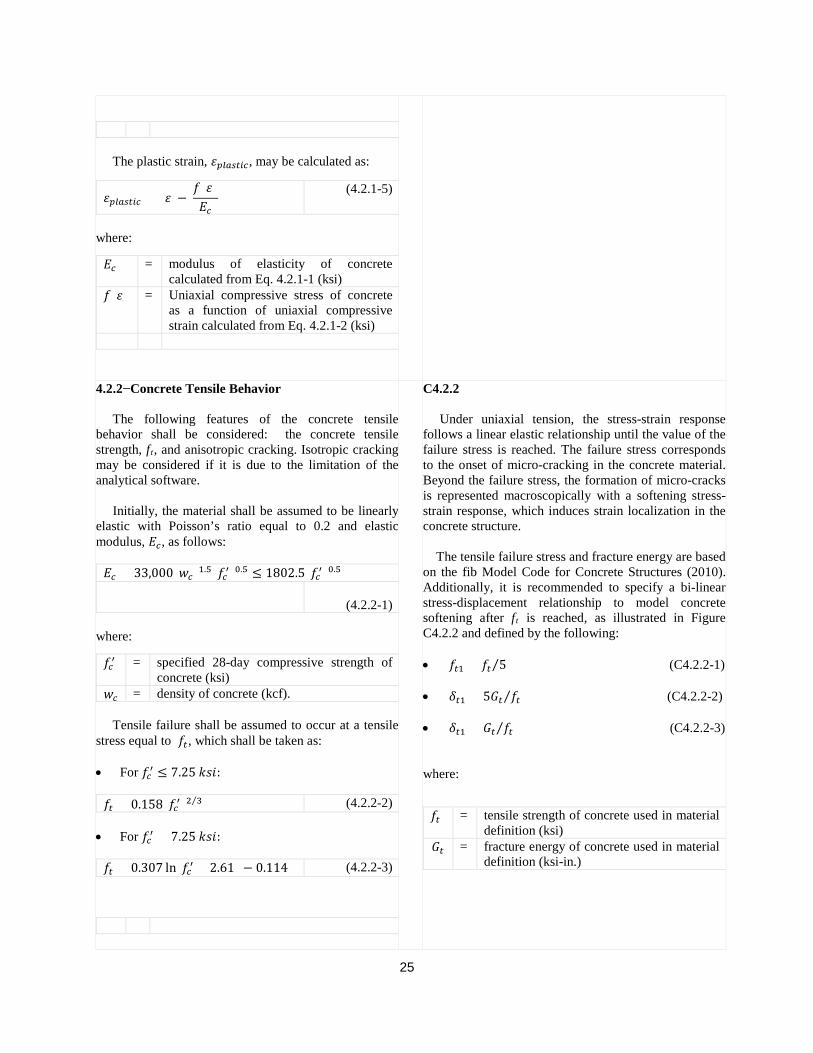
The plastic strain, 𝜀𝜀𝑝𝑝𝑝𝑝𝑝𝑝𝑠𝑠𝑝𝑝𝑝𝑝𝑐𝑐, may be calculated as:
where:
𝜀𝜀𝑝𝑝𝑝𝑝𝑝𝑝𝑠𝑠𝑝𝑝𝑝𝑝𝑐𝑐 = 𝜀𝜀 − 𝑓𝑓(𝜀𝜀)𝐸𝐸𝑐𝑐
(4.2.1-5)
𝐸𝐸𝑐𝑐 = modulus of elasticity of concrete calculated from Eq. 4.2.1-1 (ksi)
𝑓𝑓(𝜀𝜀) = Uniaxial compressive stress of concrete as a function of uniaxial compressive strain calculated from Eq. 4.2.1-2 (ksi)
4.2.2−Concrete Tensile Behavior The following features of the concrete tensile behavior shall be considered: the concrete tensile strength, ft, and anisotropic cracking. Isotropic cracking may be considered if it is due to the limitation of the analytical software. Initially, the material shall be assumed to be linearly elastic with Poisson’s ratio equal to 0.2 and elastic modulus, 𝐸𝐸𝑐𝑐, as follows:
where:
Tensile failure shall be assumed to occur at a tensile stress equal to 𝑓𝑓𝑝𝑝, which shall be taken as: • For 𝑓𝑓𝑐𝑐′ ≤ 7.25 𝑘𝑘𝑘𝑘𝑘𝑘:
• For 𝑓𝑓𝑐𝑐′ > 7.25 𝑘𝑘𝑘𝑘𝑘𝑘:
𝐸𝐸𝑐𝑐 = 33,000(𝑤𝑤𝑐𝑐)1.5(𝑓𝑓𝑐𝑐′)0.5 ≤ 1802.5(𝑓𝑓𝑐𝑐′)0.5
(4.2.2-1)
𝑓𝑓𝑐𝑐′ = specified 28-day compressive strength of concrete (ksi)
𝑤𝑤𝑐𝑐 = density of concrete (kcf).
𝑓𝑓𝑝𝑝 = 0.158(𝑓𝑓𝑐𝑐′)2 3⁄ (4.2.2-2)
𝑓𝑓𝑝𝑝 = 0.307 ln(𝑓𝑓𝑐𝑐′ + 2.61) − 0.114 (4.2.2-3)
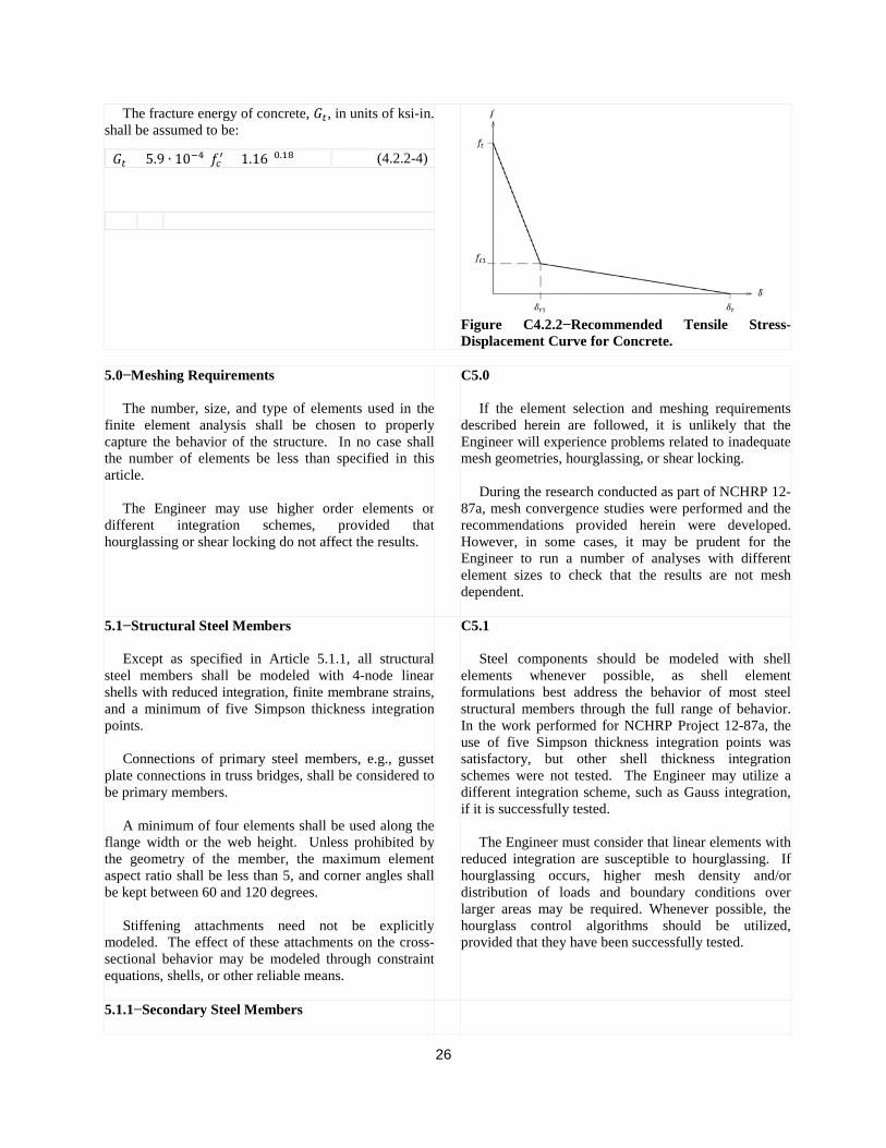
C4.2.2 Under uniaxial tension, the stress-strain response follows a linear elastic relationship until the value of the failure stress is reached. The failure stress corresponds to the onset of micro-cracking in the concrete material. Beyond the failure stress, the formation of micro-cracks is represented macroscopically with a softening stress-strain response, which induces strain localization in the concrete structure. The tensile failure stress and fracture energy are based on the fib Model Code for Concrete Structures (2010). Additionally, it is recommended to specify a bi-linear stress-displacement relationship to model concrete softening after ft is reached, as illustrated in Figure C4.2.2 and defined by the following: • 𝑓𝑓𝑝𝑝1 = 𝑓𝑓𝑝𝑝 5⁄ (C4.2.2-1) • 𝛿𝛿𝑝𝑝1 = 5𝐺𝐺𝑝𝑝 𝑓𝑓𝑝𝑝⁄ (C4.2.2-2) • 𝛿𝛿𝑝𝑝1 = 𝐺𝐺𝑝𝑝 𝑓𝑓𝑝𝑝⁄ (C4.2.2-3)
where:
𝑓𝑓𝑝𝑝 = tensile strength of concrete used in material definition (ksi)
𝐺𝐺𝑝𝑝 = fracture energy of concrete used in material definition (ksi-in.)
26
The fracture energy of concrete, 𝐺𝐺𝑝𝑝, in units of ksi-in. shall be assumed to be:
𝐺𝐺𝑝𝑝 = 5.9 ∙ 10−4(𝑓𝑓𝑐𝑐′ + 1.16)0.18 (4.2.2-4)
Figure C4.2.2−Recommended Tensile Stress-Displacement Curve for Concrete.
5.0−Meshing Requirements The number, size, and type of elements used in the finite element analysis shall be chosen to properly capture the behavior of the structure. In no case shall the number of elements be less than specified in this article. The Engineer may use higher order elements or different integration schemes, provided that hourglassing or shear locking do not affect the results.
C5.0 If the element selection and meshing requirements described herein are followed, it is unlikely that the Engineer will experience problems related to inadequate mesh geometries, hourglassing, or shear locking. During the research conducted as part of NCHRP 12-87a, mesh convergence studies were performed and the recommendations provided herein were developed. However, in some cases, it may be prudent for the Engineer to run a number of analyses with different element sizes to check that the results are not mesh dependent.
5.1−Structural Steel Members Except as specified in Article 5.1.1, all structural steel members shall be modeled with 4-node linear shells with reduced integration, finite membrane strains, and a minimum of five Simpson thickness integration points. Connections of primary steel members, e.g., gusset plate connections in truss bridges, shall be considered to be primary members. A minimum of four elements shall be used along the flange width or the web height. Unless prohibited by the geometry of the member, the maximum element aspect ratio shall be less than 5, and corner angles shall be kept between 60 and 120 degrees. Stiffening attachments need not be explicitly modeled. The effect of these attachments on the cross-sectional behavior may be modeled through constraint equations, shells, or other reliable means.
C5.1 Steel components should be modeled with shell elements whenever possible, as shell element formulations best address the behavior of most steel structural members through the full range of behavior. In the work performed for NCHRP Project 12-87a, the use of five Simpson thickness integration points was satisfactory, but other shell thickness integration schemes were not tested. The Engineer may utilize a different integration scheme, such as Gauss integration, if it is successfully tested. The Engineer must consider that linear elements with reduced integration are susceptible to hourglassing. If hourglassing occurs, higher mesh density and/or distribution of loads and boundary conditions over larger areas may be required. Whenever possible, the hourglass control algorithms should be utilized, provided that they have been successfully tested.
5.1.1−Secondary Steel Members
27
Secondary steel members that are not in contact with the concrete slab may be modeled with 2-node linear shear-flexible beam elements. A minimum of three elements shall be used along the length of the member. The following members may be considered secondary for the application of these provisions: • Lateral braces, sway braces, and cross-frames or
diaphragms; • Chords and diagonals in truss-bridge floor beams; • Construction braces. 5.2−Reinforced Concrete Slab The reinforced concrete slab may be modeled by one of the following two approaches: • Using solid elements to model the concrete, and
embedded wire elements to model the reinforcement, as specified in Article 5.2.1.
• Using shell elements in which the effect of the
layers of reinforcements is implicitly included, as specified in Article 5.2.2.
5.2.1−Reinforced Concrete Slab Modeling with Solid and Wire Elements The elements modeling the concrete slab shall be 8-node linear brick elements with reduced integration. The material model of the solid elements shall model the behavior of concrete. A minimum of eight elements shall be used through the thickness of the slab in the regions close to the fracture, which is generally within a distance of one half the width of the deck on each side of the failure location. Fewer elements may be used through the thickness in other regions, but no fewer than four shall be used. The maximum element aspect ratio shall be less than 5. Unless prohibited by the geometry of the slab, corner angles shall be kept between 40 and 140 degrees. At the locations in contact with steelwork, e.g., bottom slab haunches, the mesh density should be higher than the mesh density of the steelwork to ensure proper enforcement of the contact interaction. The reinforcing steel within the slab shall be modeled by using wire elements embedded within the solid elements. The material model of the wire elements shall model the behavior of the steel rebar. The elements shall be 2-node linear truss elements. The length of the wire
C5.2.1 Modeling the reinforced concrete slab with solid elements and embedded wire elements is the most accurate procedure, but it typically results in very large meshes that greatly increase the computational resources to perform the analysis. A minimum of eight elements must be used through the thickness of the slab so that flexure is properly captured. However, the Engineer must consider that linear elements with reduced integration are susceptible to hourglassing. If hourglassing occurs, higher mesh density and/or distribution of loads and boundary conditions over larger areas may be required. Whenever possible, the hourglass control algorithms should be utilized, provided that they have been successfully tested.

28
elements shall be approximately equal to the largest dimension of the concrete element. Concrete barriers and their reinforcement may be included as part of the slab system. 5.2.2−Reinforced Concrete Slab Modeling with Shell Elements The elements modeling the reinforced concrete slab shall be 4-node linear shells with reduced integration, finite membrane strains, and a minimum of 5 Simpson thickness integration points. The effect of the reinforcement shall be included as a material property or in the integration of the shell section. The Engineer shall test the performance of the shell element when the effects of the reinforcement are included in the element formulation, and verify that the nominal shear resistance of the slab is not exceeded. In general, the mesh density shall be similar to the one utilized for the steel elements. At the locations in contact with steelwork, e.g., bottom slab haunches, the mesh density should be higher than the mesh density of the steelwork to ensure proper enforcement of the contact interaction. Haunches may be modeled with additional superimposed layers of shell elements.
C5.2.2 In the work performed for NCHRP Project 12-87a, the use of 5 Simpson thickness integration points was satisfactory, but other shell thickness integration schemes were not tested. The Engineer may utilize a different integration scheme, such as Gauss integration, if it is successfully tested. Each layer of reinforcement may be assumed to act uniaxially, and may be treated as a smeared layer with a constant thickness equal to the area of each reinforcing bar divided by the reinforcing bar spacing. The use of concrete damage plasticity as the material model for shell elements is not effective for modeling inelastic shear behavior. Concrete damage plasticity is intended for flexural problems as the two assumed damage mechanisms are tensile cracking and compressive crushing. Shear-related damage is not directly defined in concrete damage plasticity; hence, it will not be accounted for during the shell element integration. The Engineer must consider that linear elements with reduced integration are susceptible to hourglassing. If hourglassing occurs, higher mesh density and/or distribution of loads and boundary conditions over larger areas may be required. Whenever possible, the hourglass control algorithms should be utilized, provided that they have been successfully tested.
29
6.0−Interactions and Constraints
6.1−Contact Interaction between Slab and Structural Steel Members The contact interaction between the slab and the structural steel members shall be explicitly modeled. The effects of the shear connectors shall be modeled separately as specified in Article 6.2. The normal behavior shall follow a hard pressure-overclosure relation and allow separation after contact. The tangential behavior shall be modeled with a Coulomb frictional model. The coefficient of friction shall be taken as 0.55 and the interfacial shear limit shall be taken as 0.06 ksi, unless experimental evidence supports otherwise.
C6.1 Contact interactions are intended to model the transfer of normal compressive forces and tangential frictional shear forces between the steelwork and the slab. Any other source of force transfer, such as that provided by shear connectors, must be considered separately.
6.2−Composite Action between the Slab and Structural Steel Members When modeling shear studs, the tensile, shear, and combined shear and axial load-displacement behavior of the shear stud shall be considered in the analysis. The methodology to calculate the stiffness, strength, and ductility of transversely grouped shear studs is specified in Articles 6.2.1 through 6.2.3. The methodology shall be considered valid for groups of one, two, or three shear studs.
C6.2 The research conducted in NCHRP Project 12-87a found that the behavior of shear studs needs to be properly modeled to capture the transfer of load from a faulted composite girder to the rest of the structure. Shear stud failure is possible in the faulted state, typically in tension by concrete breakout, which reduces composite action and affects the development of alternative load paths. The girder systems studied in NCHRP Project 12-87a and Korkmaz et al. (2017) had a maximum of three shear studs spaced transversely. Additional research is necessary to develop recommendations for four or more transversely grouped shear studs.
6.2.1−Shear Behavior of Transversely Grouped Shear Studs The shear strength of transversely grouped shear studs is based on the nominal shear resistance for a single stud embedded in concrete, 𝑄𝑄𝑛𝑛, specified in LRFD Design Article 6.10.10.4.3. The shear force-displacement relationship for a shear stud group embedded in concrete based on the shear as a function of the shear displacement for a shear stud group, 𝑄𝑄𝑔𝑔(𝛿𝛿𝑄𝑄), shall be calculated as follows:
where:
𝑄𝑄𝑔𝑔(𝛿𝛿𝑄𝑄) = 𝑄𝑄𝑔𝑔,𝑛𝑛(1 − 𝑒𝑒−18𝛿𝛿𝑄𝑄)2/5 (6.2.1-1)
𝑄𝑄𝑔𝑔,𝑛𝑛 = nominal shear resistance of a group of shear studs embedded in a concrete slab (kip)
𝛿𝛿𝑄𝑄 = shear displacement of a shear stud (in.)
C6.2.1 The shear force-displacement behavior is based on the model described by Ollgaard et al. (1971). The maximum cumulative shear displacement is limited to 0.2 in., which is equal to 90% of the shear capacity according to Ollgaard et al. (1971).

30
The nominal shear resistance of a group of shear studs embedded in a concrete slab, 𝑄𝑄𝑔𝑔,𝑛𝑛, shall be taken as follows:
where;
Failure of the shear stud group shall be assumed to occur at a shear displacement, 𝛿𝛿𝑄𝑄, equal to 0.2 in.
𝑄𝑄𝑔𝑔,𝑛𝑛 = 𝑄𝑄𝑛𝑛 𝑁𝑁𝑠𝑠 (6.2.1-2)
𝑁𝑁𝑠𝑠 = number of transversely grouped shear studs 𝑄𝑄𝑛𝑛 = nominal shear resistance of one shear stud
embedded in a concrete slab calculated in accordance with LRFD Design Article 6.10.10.4.3 (kip)
6.2.2−Tensile Behavior of Transversely Grouped Shear Studs To model the tensile behavior of transverse groups of one, two, or three shear studs, the following shall be calculated: • The initial stiffness of the shear stud group, 𝐾𝐾𝑔𝑔,
calculated as specified in Article 6.2.2.1. • The nominal tensile strength of the shear stud
group, 𝑁𝑁𝑔𝑔,𝑛𝑛, calculated as specified in Article 6.2.2.2.
𝐾𝐾𝑔𝑔 and 𝑁𝑁𝑔𝑔,𝑛𝑛 shall be used to develop tensile load-displacement relationships based on the tension force as a function of the axial displacement for the shear stud group, 𝑁𝑁𝑔𝑔(𝛿𝛿𝑁𝑁), calculated as specified in Article 6.2.2.3 that shall be included in the analysis.
C6.2.2 Shear studs under high tensile load may fail due to shear stud steel rupture, concrete pullout, or concrete break-out. The overall methodology to determine nominal tensile behavior is explained in Connor et al. (2017). This methodology is an adaptation of the approach given in ACI 318-14 (ACI, 2014). A detailed study was performed in NCHRP Project 12-87a to modify the equations given in ACI 318-14 (ACI, 2014), with the objective of capturing shear stud behavior in composite steel bridges. The effect of several parameters such as grouping effects, i.e., the load distribution ratio between the shear studs, flange geometry, and haunch thickness on the connector element stiffness, strength, and ductility was investigated in NCHRP Project 12-87a.
6.2.2.1−Initial Tensile Stiffness of Transversely Grouped Shear Studs The axial stiffness of a shear stud group, 𝐾𝐾𝑔𝑔, shall be calculated as follows:
in which:
𝐾𝐾𝑔𝑔 = 𝐾𝐾1𝑅𝑅𝑐𝑐 (6.2.2.1-1)
𝐾𝐾1 = single stud cumulative stiffness neglecting the effect of flange flexibility (kip/in.). Calculated as follows:
𝐾𝐾1 = [(𝐾𝐾𝑐𝑐1)−1 + (𝐾𝐾𝑠𝑠1)−1]−1 (6.2.2.1-2)
C6.2.2.1 The axial stiffness of a shear stud group is calculated taking into consideration the combined effect of the stiffness of the shear stud shaft, the stiffness of the concrete section affected by the shear stud, and the bending stiffness of the flange.
31
where:
The shear stud group stiffness coefficient, 𝑅𝑅𝑐𝑐, for the calculation of the axial stiffness of a shear stud group shall be taken as: • For one transversely grouped stud:
• For two transversely grouped studs:
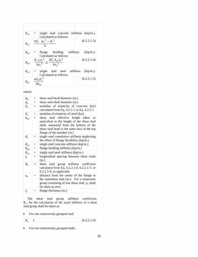
𝐾𝐾𝑐𝑐1 = single stud concrete stiffness (kip/in.). Calculated as follows:
𝐾𝐾𝑐𝑐1 =𝜋𝜋𝐸𝐸𝑐𝑐 (𝑑𝑑ℎ
2 − 𝑑𝑑𝑠𝑠2)
5
(6.2.2.1-3)
𝐾𝐾𝑝𝑝1 = flange bending stiffness (kip/in.). Calculated as follows:
𝐾𝐾𝑝𝑝1 =𝐸𝐸𝑠𝑠 𝑙𝑙𝑠𝑠𝑡𝑡𝑓𝑓3
4𝑘𝑘𝑜𝑜3≤
3𝐸𝐸𝑠𝑠 ℎ𝑒𝑒𝑓𝑓𝑡𝑡𝑓𝑓3
4𝑘𝑘𝑜𝑜3
(6.2.2.1-4)
𝐾𝐾𝑠𝑠1 = single stud steel stiffness (kip/in.). Calculated as follows:
𝐾𝐾𝑠𝑠1 =𝜋𝜋𝐸𝐸𝑠𝑠𝑑𝑑𝑠𝑠
2
4ℎ𝑒𝑒𝑓𝑓
(6.2.2.1-5)
𝑑𝑑ℎ = shear stud head diameter (in.) 𝑑𝑑𝑠𝑠 = shear stud shaft diameter (in.) 𝐸𝐸𝑐𝑐 = modulus of elasticity of concrete (ksi)
calculated from Eq. 4.2.1-1 or Eq. 4.2.2-1 𝐸𝐸𝑠𝑠 = modulus of elasticity of steel (ksi). ℎ𝑒𝑒𝑓𝑓 = shear stud effective height taken as
equivalent to the height of the shear stud shaft, measured from the bottom of the shear stud head to the outer face of the top flange of the member (in.)
𝐾𝐾1 = single stud cumulative stiffness neglecting the effect of flange flexibility (kip/in.)
𝐾𝐾𝑐𝑐1 = single stud concrete stiffness (kip/in.) 𝐾𝐾𝑝𝑝1 = flange bending stiffness (kip/in.) 𝐾𝐾𝑠𝑠1 = single stud steel stiffness (kip/in.) 𝑙𝑙𝑠𝑠 = longitudinal spacing between shear studs
(in.) 𝑅𝑅𝑐𝑐 = shear stud group stiffness coefficient
calculated from Eq. 6.2.2.1-6, 6.2.2.1-7, or 6.2.2.1-8, as applicable
𝑘𝑘0 = distance from the center of the flange to the outermost stud (in.). For a transverse group consisting of one shear stud, 𝑘𝑘0 shall be taken as zero.
𝑡𝑡𝑓𝑓 = flange thickness (in.)
𝑅𝑅𝑐𝑐 = 1 (6.2.2.1-6)

32
• For three transversely grouped shear studs:
𝑅𝑅𝑐𝑐 =2𝐾𝐾𝑝𝑝1(𝐾𝐾𝑐𝑐1 + 𝐾𝐾𝑠𝑠1)
𝐾𝐾𝑝𝑝1(𝐾𝐾𝑐𝑐1 + 𝐾𝐾𝑠𝑠1) + 𝐾𝐾𝑐𝑐1𝐾𝐾𝑠𝑠1
(6.2.2.1-7)
𝑅𝑅𝑐𝑐 =𝐾𝐾1 + 3𝐾𝐾𝑝𝑝1𝐾𝐾1 + 𝐾𝐾𝑝𝑝1
(6.2.2.1-8)
6.2.2.2−Tensile Strength of Transversely Grouped Shear Studs For composite bridges, the nominal tensile strength of a shear stud group embedded in concrete, 𝑁𝑁𝑔𝑔,𝑛𝑛, shall be calculated as the minimum of the tensile rupture strength, 𝑁𝑁𝑠𝑠𝑝𝑝, the pullout strength, 𝑁𝑁𝑝𝑝𝑛𝑛, and the concrete break-out strength, 𝑁𝑁𝑐𝑐𝑏𝑏 , or:
The tensile rupture strength of transversely grouped shear studs, 𝑁𝑁𝑠𝑠𝑝𝑝, shall be calculated as follows:
where:
The distribution factor for shear stud groups, 𝑆𝑆𝑁𝑁, for the calculation of the tensile rupture strength and the pullout strength of transversely grouped shear studs shall be taken as: • For one transversely grouped stud:
• For two transversely grouped studs:
• For three transversely grouped studs:
𝑁𝑁𝑔𝑔,𝑛𝑛 = min�𝑁𝑁𝑠𝑠𝑝𝑝 ,𝑁𝑁𝑝𝑝𝑛𝑛,𝑁𝑁𝑐𝑐𝑏𝑏� (6.2.2.2-1)
𝑁𝑁𝑠𝑠𝑝𝑝 = 𝑁𝑁𝑠𝑠 𝐷𝐷𝑠𝑠𝑒𝑒,𝑁𝑁𝑓𝑓𝑦𝑦𝑝𝑝 + 𝑆𝑆𝑁𝑁(𝑓𝑓𝑢𝑢𝑝𝑝 − 𝑓𝑓𝑦𝑦𝑝𝑝)𝐷𝐷𝑠𝑠𝑒𝑒,𝑁𝑁
(6.2.2.2-2)
𝐷𝐷𝑠𝑠𝑒𝑒,𝑁𝑁 = effective cross-sectional area of a single stud (in.2)
𝑓𝑓𝑢𝑢𝑝𝑝 = nominal ultimate strength of the stud (ksi)
𝑓𝑓𝑦𝑦𝑝𝑝 = nominal yield strength of the stud (ksi) 𝑁𝑁𝑠𝑠 = number of transversely grouped shear
studs 𝑆𝑆𝑁𝑁 = distribution factor for shear stud groups
calculated from Eq. 6.2.2.2-3, 6.2.2.2-4, or 6.2.2.2-5, as applicable
𝑆𝑆𝑁𝑁 = 1 (6.2.2.2-3)
𝑆𝑆𝑁𝑁 = 2 (6.2.2.2-4)
C6.2.2.2 The pullout strength and concrete break-out equations are based on 5% fractile calculations for the available test sample. Concrete cracking modification factors, 𝜓𝜓c,P and 𝜓𝜓c,N, are determined according to the ACI 318-14 (ACI, 2014) procedure. In the Redundancy II load combination, it is generally assumed that the bridge has been in the faulted state for some finite period of time. Therefore, regardless of cracking at service load levels, the Engineer may wish to conservatively take 𝜓𝜓c,P and 𝜓𝜓c,N as 1.0.
33
where 𝐾𝐾1 and 𝐾𝐾𝑝𝑝1 shall be taken as specified in Article 6.2.2.1. The pullout strength of transversely grouped shear studs, 𝑁𝑁𝑝𝑝𝑛𝑛, shall only be considered if the following relationship is satisfied:
in which case, 𝑁𝑁𝑝𝑝𝑛𝑛 shall be calculated as follows:
where:
The cracking modification factor for the calculation of the pullout strength of transversely grouped shear studs, 𝜓𝜓𝑐𝑐,𝑃𝑃, shall be taken as: • When cracking is not expected at service load
levels:
• When cracking is expected at service load levels:
The concrete break-out strength of transversely grouped shear studs, 𝑁𝑁𝑐𝑐𝑏𝑏 , shall be calculated as follows:
where:
𝑆𝑆𝑁𝑁 =𝐾𝐾1 + 3𝐾𝐾𝑝𝑝1𝐾𝐾1 + 𝐾𝐾𝑝𝑝1
(6.2.2.2-5)
𝜓𝜓𝑐𝑐,𝑃𝑃�8𝐷𝐷𝑏𝑏𝑏𝑏𝑔𝑔𝑓𝑓𝑐𝑐′� < 𝐷𝐷𝑠𝑠𝑒𝑒,𝑁𝑁𝑓𝑓𝑢𝑢𝑝𝑝 (6.2.2.2-6)
𝑁𝑁𝑝𝑝𝑛𝑛 = 𝑆𝑆𝑁𝑁𝜓𝜓𝑐𝑐,𝑃𝑃(8𝐷𝐷𝑏𝑏𝑏𝑏𝑔𝑔𝑓𝑓𝑐𝑐′) (6.2.2.2-7)
𝐷𝐷𝑏𝑏𝑏𝑏𝑔𝑔 = under-head cross-sectional net area of a single stud (in.2)
𝑓𝑓𝑐𝑐′ = specified 28-day compressive strength of concrete (ksi)
𝜓𝜓𝑐𝑐,𝑃𝑃 = cracking modification factor calculated
from Eq. 6.2.2.2-8 or 6.2.2.2-9, as applicable
𝜓𝜓𝑐𝑐,𝑃𝑃 = 1.4 (6.2.2.2-8)
𝜓𝜓𝑐𝑐,𝑃𝑃 = 1.0 (6.2.2.2-9)
𝑁𝑁𝑐𝑐𝑏𝑏 =2𝑙𝑙𝑠𝑠(𝑐𝑐1 + 𝑘𝑘0)𝜓𝜓𝑒𝑒𝑒𝑒 ,𝑁𝑁𝜓𝜓𝑐𝑐,𝑁𝑁𝑁𝑁𝑏𝑏
9ℎ𝑒𝑒𝑓𝑓2
≤2(𝑐𝑐1 + 𝑘𝑘0)𝜓𝜓𝑒𝑒𝑒𝑒,𝑁𝑁𝜓𝜓𝑐𝑐,𝑁𝑁𝑁𝑁𝑏𝑏
3ℎ𝑒𝑒𝑓𝑓
(6.2.2.2-10)
𝑐𝑐1 = effective edge distance calculated from Eq. 6.2.2.2-12 (in.)

34
The non-modified concrete break-out strength of a single shear stud, 𝑁𝑁𝑏𝑏, for the calculation of the concrete break-out strength of transversely grouped shear studs shall be taken as:
The effective edge distance, 𝑐𝑐1, for the calculation of the concrete break-out strength of transversely grouped shear studs shall be taken as:
where:
The edge modification factor, 𝜓𝜓𝑒𝑒𝑒𝑒,𝑁𝑁, for the calculation of the concrete break-out strength of transversely grouped shear studs shall be taken as:
ℎ𝑒𝑒𝑓𝑓 = shear stud effective height taken as equivalent to the height of the shear stud shaft, measured from the bottom of the shear stud head to the outer face of the top flange of the member (in.)
𝑙𝑙𝑠𝑠 = longitudinal spacing between shear studs (in.)
𝑁𝑁𝑏𝑏 = Non-modified concrete break-out strength of a single shear stud calculated from Eq. 6.2.2.2-11 (kip)
𝑘𝑘0 = Distance from the center of the flange to the outermost stud (in.). For a transverse group consisting of one shear stud, 𝑘𝑘0 shall be taken as zero.
𝜓𝜓𝑐𝑐,𝑁𝑁 = cracking modification factor calculated from Eq. 6.2.2.2-14 or 6.2.2.2-15, as applicable
𝜓𝜓𝑒𝑒𝑒𝑒,𝑁𝑁 = edge modification factor calculated from Eq. 6.2.2.2-13
𝑁𝑁𝑏𝑏 = 0.759(𝑓𝑓𝑐𝑐′)0.5ℎ𝑒𝑒𝑓𝑓1.5 (6.2.2.2-11)
𝑐𝑐1 = max[1.5(ℎ𝑒𝑒𝑓𝑓 − 𝑡𝑡ℎ) , 0.5𝑤𝑤ℎ − 𝑘𝑘𝑜𝑜 ] ≤ 1.5ℎ𝑒𝑒𝑓𝑓
(6.2.2.2-12)
𝑡𝑡ℎ = net haunch thickness measured from top
of top flange to underside of slab (in.) 𝑤𝑤ℎ = haunch width (in.)
𝜓𝜓𝑒𝑒𝑒𝑒,𝑁𝑁 = 0.7 + 0.3𝑐𝑐1
1.5ℎ𝑒𝑒𝑓𝑓 ≤ 1.0 (6.2.2.2-13)
35
The cracking modification factor, 𝜓𝜓𝑐𝑐,𝑁𝑁, for the calculation of the break-out strength of transversely grouped shear studs shall be taken as: • When cracking is not expected at service load
levels:
• When cracking is expected at service load levels:
𝜓𝜓𝑐𝑐,𝑁𝑁 = 1.25 (6.2.2.2-14)
𝜓𝜓𝑐𝑐,𝑁𝑁 = 1.0 (6.2.2.2-15)
6.2.2.3−Load-Displacement Relationships of Transversely Grouped Shear Studs in Tension If the governing failure mode is tensile rupture, i.e., 𝑁𝑁𝑔𝑔,𝑛𝑛 = 𝑁𝑁𝑠𝑠𝑝𝑝, the tension force as a function of axial displacement for transversely grouped shear studs, 𝑁𝑁𝑔𝑔(𝛿𝛿𝑁𝑁), shall be calculated as follows: • For 𝛿𝛿𝑁𝑁 ≤
𝑁𝑁𝑦𝑦𝑦𝑦𝐾𝐾𝑔𝑔
:
• For 𝑁𝑁𝑦𝑦𝑦𝑦
𝐾𝐾𝑔𝑔< 𝛿𝛿𝑁𝑁 ≤ 0.05ℎ𝑒𝑒𝑓𝑓:
where:
𝑁𝑁𝑔𝑔(𝛿𝛿𝑁𝑁) = 𝐾𝐾𝑔𝑔 𝛿𝛿𝑁𝑁 (6.2.2.3-1)
𝑁𝑁𝑔𝑔(𝛿𝛿𝑁𝑁) = 𝑁𝑁𝑦𝑦𝑝𝑝 + �𝛿𝛿𝑁𝑁 −
𝑁𝑁𝑦𝑦𝑝𝑝𝐾𝐾𝑔𝑔
� �𝑁𝑁𝑔𝑔,𝑛𝑛 − 𝑁𝑁𝑦𝑦𝑝𝑝�
0.05ℎ𝑒𝑒𝑓𝑓 − 𝑁𝑁𝑦𝑦𝑝𝑝𝐾𝐾𝑔𝑔
(6.2.2.3-2)
ℎ𝑒𝑒𝑓𝑓 = shear stud effective height taken as equivalent to the height of the shear stud shaft, measured from the bottom of the shear stud head to the outer face of the top flange of the member (in.)
𝐾𝐾𝑔𝑔 = axial stiffness of the shear stud group calculated from Eq. 6.2.2.1-1 (kip/in.)
𝑁𝑁𝑔𝑔,𝑛𝑛 = nominal tensile strength of the shear stud group calculated from Eq. 6.2.2.2-1 (kip)
Nsa = tensile rupture strength of transversely grouped shear studs calculated from Eq. 6.2.2.2-2 (kip)
C6.2.2.3 The behavior of transversely grouped shear studs in tension is dependent upon the governing failure mode. The tensile behavior of a shear stud group when the governing failure mode is tensile rupture of the shear stud shaft can be characterized as follows: • Initially linearly elastic behavior with a stiffness,
𝐾𝐾𝑔𝑔, until the yield strength of the shear stud group, 𝑁𝑁𝑦𝑦𝑝𝑝, is reached;
• Once 𝑁𝑁𝑦𝑦𝑝𝑝 is reached, plastic behavior with linear
hardening until the rupture strength of the shear stud shaft, 𝑁𝑁𝑠𝑠𝑝𝑝, is reached;
• Once 𝑁𝑁𝑠𝑠𝑝𝑝 is reached, the shear stud group is
assumed to fail. The axial displacement at failure is conservatively assumed to be 5% of the effective height of the shear stud, ℎ𝑒𝑒𝑓𝑓 .

36
The tensile yield strength of transversely grouped shear studs, 𝑁𝑁𝑦𝑦𝑝𝑝,.shall be taken as follows:
where:
Failure of the shear stud group shall be assumed to occur once 𝛿𝛿𝑁𝑁 reaches0.05ℎ𝑒𝑒𝑓𝑓 . If the governing failure mode is shear stud pullout, i.e., 𝑁𝑁𝑔𝑔,𝑛𝑛 = 𝑁𝑁𝑝𝑝𝑛𝑛, or concrete break-out, i.e., 𝑁𝑁𝑔𝑔,𝑛𝑛 = 𝑁𝑁𝑐𝑐𝑏𝑏 , the tension force as a function of the axial displacement for transversely grouped shear studs, 𝑁𝑁𝑔𝑔(𝛿𝛿𝑁𝑁), shall be calculated as follows: • For 𝛿𝛿𝑁𝑁 ≤
𝑁𝑁𝑔𝑔,𝑛𝑛
𝐾𝐾𝑔𝑔:
• For 𝑁𝑁𝑔𝑔,𝑛𝑛
𝐾𝐾𝑔𝑔< 𝛿𝛿𝑁𝑁 ≤ 𝛿𝛿𝑁𝑁,𝑓𝑓:
where:
The tensile displacement of a shear stud group at failure for the shear stud pullout or concrete break-out failure modes, 𝛿𝛿𝑁𝑁,𝑓𝑓, shall be taken as follows: • For on transversely grouped shear stud:
𝑁𝑁𝑦𝑦𝑝𝑝 = tensile yield strength of transversely grouped shear studs calculated from Eq. 6.2.2.3-3 (kip)
𝛿𝛿𝑁𝑁 = tensile displacement of a shear stud (in.)
𝑁𝑁𝑦𝑦𝑝𝑝 = 𝑁𝑁𝑠𝑠 𝐷𝐷𝑠𝑠𝑒𝑒,𝑁𝑁 𝑓𝑓𝑦𝑦𝑝𝑝 (6.2.2.3-3)
𝐷𝐷𝑠𝑠𝑒𝑒,𝑁𝑁 = effective cross-sectional area of a single stud (in.2)
𝑓𝑓𝑦𝑦𝑝𝑝 = specified minimum yield strength of the stud (ksi)
𝑁𝑁𝑠𝑠 = number of transversely grouped shear studs
𝑁𝑁𝑔𝑔(𝛿𝛿𝑁𝑁) = 𝐾𝐾𝑔𝑔 𝛿𝛿𝑁𝑁 (6.2.2.3-4)
𝑁𝑁𝑔𝑔(𝛿𝛿𝑁𝑁) = 𝐾𝐾𝑔𝑔 𝑁𝑁𝑔𝑔,𝑛𝑛𝛿𝛿𝑁𝑁,𝑓𝑓 − 𝛿𝛿𝑁𝑁
𝐾𝐾𝑔𝑔𝛿𝛿𝑁𝑁,𝑓𝑓 − 𝑁𝑁𝑔𝑔,𝑛𝑛
(6.2.2.3-5)
𝛿𝛿𝑁𝑁,𝑓𝑓 = tensile displacement of a shear stud group
at failure for shear stud pullout or concrete break-out failure modes calculated from Eq. 6.2.2.3-6, 6.2.2.3-7, or 6.2.2.3-8, as applicable (in.)
The tensile behavior of a shear stud group when the governing failure mode is shear stud pullout or concrete break-out can be characterized as follows: • Initially linearly elastic behavior with a stiffness,
𝐾𝐾𝑔𝑔, until the pullout strength or concrete break-out of the shear stud group, 𝑁𝑁𝑝𝑝𝑛𝑛 or 𝑁𝑁𝑐𝑐𝑏𝑏 , is reached;
• Once 𝑁𝑁𝑝𝑝𝑛𝑛 or 𝑁𝑁𝑐𝑐𝑏𝑏 is reached, linear softening until
the ductility of the shear stud assembly is exhausted.

37
• For two transversely grouped shear studs:
• For three transversely grouped shear studs:
Failure of the shear stud group shall be assumed to occur once 𝛿𝛿𝑁𝑁 reaches 𝛿𝛿𝑁𝑁,𝑓𝑓.
𝛿𝛿𝑁𝑁,𝑓𝑓 = 20𝑁𝑁𝑔𝑔,𝑛𝑛
𝐾𝐾𝑔𝑔
(6.2.2.3-6)
𝛿𝛿𝑁𝑁,𝑓𝑓 = 7.5𝑁𝑁𝑔𝑔,𝑛𝑛
𝐾𝐾𝑔𝑔
(6.2.2.3-7)
𝛿𝛿𝑁𝑁,𝑓𝑓 = 6.4𝑁𝑁𝑔𝑔,𝑛𝑛
𝐾𝐾𝑔𝑔
(6.2.2.3-8)
6.2.3−Combined Shear and Tension The combined effects of tension and shear in shear studs shall be considered if either of the following is true:
where:
𝑁𝑁𝑔𝑔(𝛿𝛿𝑁𝑁)𝑁𝑁𝑔𝑔,𝑛𝑛
> 0.2 (6.2.3-1)
𝑄𝑄𝑔𝑔�𝛿𝛿𝑄𝑄�𝑄𝑄𝑔𝑔,𝑛𝑛
> 0.2 (6.2.3-2)
𝑁𝑁𝑔𝑔,𝑛𝑛 = nominal tensile strength of the shear stud group embedded in a concrete slab calculated from Eq. 6.2.2.2-1
𝑁𝑁𝑔𝑔(𝛿𝛿𝑁𝑁) = tension force as a function of the axial displacement for a shear stud group embedded in concrete calculated as specified in Article 6.2.2.3 (kip)
𝑄𝑄𝑔𝑔,𝑛𝑛 = nominal shear resistance of a group of shear studs embedded in a concrete slab calculated from Eq. 6.2.1-2 (kip)
𝑄𝑄𝑔𝑔�𝛿𝛿𝑄𝑄� = shear as a function of the shear displacement for a shear stud group embedded in concrete calculated from Eq. 6.2.1-1 (kip)
C6.2.3 The following tension-shear interaction equation is adapted from LRFD Design Equation 6.16.4.3-1 (AASHTO, 2017) may used to combine the effects of tension and shear in shear stud groups.
where:
The application of Equation C6.2.3-1 in FEA may be complex and simplifications may be required depending on the FEA solver used. The Engineer is strongly encouraged to review Appendix A of Connor et al. (2017) for a detailed explanation of combined shear and tensile behavior of shear stud groups.
�𝑁𝑁𝑔𝑔(𝛿𝛿𝑁𝑁)𝑁𝑁𝑔𝑔,𝑛𝑛
�5 3⁄
+ �𝑄𝑄𝑔𝑔�𝛿𝛿𝑄𝑄�𝑄𝑄𝑔𝑔,𝑛𝑛
�5 3⁄
≤ 1.0 (C6.2.3-1)
𝑁𝑁𝑔𝑔,𝑛𝑛 = nominal tensile strength of the shear stud group embedded in a concrete slab calculated from Eq. 6.2.2.2-1
𝑁𝑁𝑔𝑔(𝛿𝛿𝑁𝑁) = tension force as a function of the axial displacement for a shear stud group embedded in concrete calculated as specified in Article 6.2.2.3 (kip)
𝑄𝑄𝑔𝑔,𝑛𝑛 = nominal shear resistance of a group of shear studs embedded in a concrete slab calculated from Eq. 6.2.1-2 (kip)
𝑄𝑄𝑔𝑔�𝛿𝛿𝑄𝑄� = shear as a function of the shear displacement for a shear stud group embedded in concrete calculated from Eq. 6.2.1-1 (kip)

38
6.3−Connections of Structural Steel Members Connections of structural steel members shall be modeled so that forces and moments are adequately transferred between the structural members. Whenever failure of the connection is more likely to occur than failure of the member, connection failure shall be explicitly considered in the analysis.
C6.3 When modeling the stiffness of a steel connection, it may necessary to explicitly model the geometry of the connection. In general, for a bolted connection weaker than the connected members, the behavior can be modeled by a linear-elastic perfectly-plastic relationship defined by the following: • An initial elastic stiffness which is a combination
of the axial stiffness of the plate, bearing stiffness of the plate, and the shear stiffness of the bolts. The individual stiffness values may be calculated per the provisions given in Eurocode 3 (CEN, 2007) or Henriques et al. (2014). A series sum (1/ktotal = 1/kplate + 1/kbolt + 1/kbearing) may be used to combine the individual stiffness values.
• The capacity of the connection, Rconn, may be
calculated per the provisions in the BDS. • The maximum displacement at failure may be
calculated as the largest of 2.5 times the capacity-to-stiffness ratio and 0.18 times the diameter of the bolt; i.e., umax = max(2.5·Rconn/ktotal, 0.18·db) (Sarraj, 2007).
39
7.0−Application of Loads and Boundary Conditions
7.1−Application of Loads Load application in the finite element model shall be such that inertial effects are minimized if a dynamic analysis is used. Component dead loads shall be applied as body forces to ensure proper distribution of load. Vehicular live loads shall be applied as surface tractions. Wheel footprints shall be 10 inches along the span by 20 inches across the span.
C7.1 Other loads, such as wearing surfaces or traffic signs may be included. The Engineer should avoid any source of fictitious stress concentrations or element distortion due to the application of load, as these may result in premature element failure. For example, using a point load to represent a tire footprint could result in element distortion and premature element failure. The load is applied statically or quasi-statically because any dynamic effects of the fracture event are already considered when the dynamic amplification factor, DAR, specified in Article 3.3 is applied.
7.2 Support Conditions The flexibility of the substructure and the type of support system shall be considered in the analysis. Wherever a displacement degree-of-freedom is constrained at a support location, the force-translation or/and moment-rotation behavior of the support, i.e., the substructure and associated bearing, shall be considered in the analysis. The support shall be capable of carrying the applied loads and accommodating the required displacements in the faulted state for the Redundancy I and Redundancy II load combinations specified in Article 3.4.
C7.2 The substructure needs to be capable of resisting the load and displacement demands when the redundancy of the superstructure is analyzed. Therefore, the forces and displacements computed at the support points are to be used as factored demands for checking the nominal resistance of the substructure elements. Hence, the Engineer needs to consider the flexibility of the substructure realistically. The Engineer must utilize a best estimate of the flexibility of the substructure, and should not be biased towards more rigid or softer behavior. The materials, geometry, and support conditions of the substructure components need to be considered in the flexibility calculations. Recommendations for the calculation of the nominal resistance of substructure elements can be found in Sections 10 and 11 of the BDS.

40
8.0−Performance Criteria in the Faulted State Except as specified herein, once the analysis has been performed in accordance with the provisions of Articles 3 through 7, the structure shall be evaluated in the faulted state against the strength requirements specified in Article 8.1 and the serviceability requirements specified in Article 8.2 to determine whether or not primary steel tension members are to be designated as FCMs or SRMs. If any of the attributes specified in Article 2.1 apply to the structure under evaluation, primary steel tension members in that structure shall not be designated as SRMs, except as permitted in Article 2.1.
8.1−Strength Requirements When the structure is subjected to the Redundancy I or the Redundancy II load combination specified in Article 3.4 in the faulted state, the primary steel tension members shall be designated as FCMs if one or more of the strength considerations specified in Article 8.1.1 or 8.1.2 is true. Otherwise, the primary steel tension members shall be designated as SRMs. 8.1.1−Superstructure Considerations • In a component, such as a web or a flange of a
primary steel member, the average strain is larger than five times the material yield strain.
• In a component, such as a web or a flange of a
primary steel member, the average strain is larger than 0.01.
• A strain level of 0.05 is reached anywhere in a
primary steel member. Higher strain limits are permitted when supported by experimental testing.
• The combined flexural, torsional and axial force
effects computed in primary compression members exceed the nominal compressive resistance of the member, unless these limit states are predicted by the FEA.
• The concrete slab has reached 0.003 compression
strain in a portion sufficiently large to compromise the overall system load carrying capacity.
• The system fails to support an additional 15% of the
factored live load.
C8.1 The strength requirements developed for the performance criteria are not intended to drive the design of new bridges. They were developed to establish minimum acceptable performance levels in the faulted state. Since, in this case, the evaluation is performed on the system, rather than on the member as is done in a typical bridge design, stress and strain criteria are used rather than force-effect criteria. The analyst must be conscious of the complexity of capturing the stability of individual steel components whose behavior is dominated by axial compression. Hence, steel members in compression should be analyzed in detail and their nominal resistances must be checked against the demands calculated in the redundancy evaluation. The addition of 15% more live load provides a reasonable level of additional live load that can be used to demonstrate that the load-deflection curve is still on the ascending branch. While other proportions could have been used, 15% was selected as a reasonable extension to demonstrate that the structure still has some reserve capacity based on the coefficient of variation of the HL-93 vehicular live load model beyond that provided by the Redundancy I and II load combinations. Further details pertaining to the development of these strength requirements can be found in Conner et al. (2017).
41
8.1.2−Substructure Considerations • At any support location, the reaction forces and
moments exceed the nominal resistance of a substructure element or the support system.
• The substructure fails to safely accommodate the
displacements and reactions of the superstructure in the faulted state.
C8.1.2 Transverse and longitudinal displacements at support locations should be considered in the faulted state as a member may lose support, particularly at supports that allow for expansion. Hence, it should be verified that these horizontal displacements can be accommodated by the support in the faulted state; i.e., it should be verified that the superstructure does not fall off of a support, whether that be by a bearing tipping over or a girder coming completely off of a pier or abutment.
8.2−Serviceability Requirements When the structure is subjected to the dead load portion of the Redundancy II load combination specified in Article 3.4 in the faulted state, the primary steel tension members shall be designated as FCMs if one or more of the following serviceability considerations are true. Otherwise, the primary steel tension members shall be designated as SRMs. • When considering a scenario in which failure is
assumed to occur in a longitudinal primary member, the maximum vertical deflection is larger than L/50, where L is the span length.
• When considering a scenario in which failure is
assumed to occur in a floor beam, the maximum vertical deflection of the floor beam is larger than L/50, where L is the distance between floor beams that are assumed not to have failed.
C8.2 Changes in geometry of the structure in the faulted state need to be limited to ensure traffic can safely cross the structure during the extended service period immediately following the fracture. The development of the performance criteria are discussed more fully in Connor et al. (2017). Based on a review of several case studies, it appears that substantial vertical deflections comparable to the specified limit can be tolerated by motorists without impact to the traveling public’s safety, at least in the short term. In cases where there is very little deflection, the damage may go undetected for an extended period of time. In some cases, very localized deflections in the slab may occur. However, such localized deflections are not intended to be evaluated with the L/50 limit. The deflection limit for floor beams is intended to ensure that excessive sagging does not occur between floor beams. For example, if floor beams are uniformly spaced at 20 feet along the span, L should be taken as 40 feet. Since the deflection due to dead load is of concern, the dead load portion of the Redundancy II load combination is to be used to evaluate the serviceability requirements specified herein since it does not include the effects of the dynamic amplification factor, 𝐷𝐷𝐷𝐷𝑅𝑅 , specified in Article 3.3. The Engineer may need to consider additional serviceability requirements. One particular concern is the actual detectability of the failure in a primary steel member in the faulted state, as there are multiple cases

42
of bridges in which a member designated as a FCM failed and traffic continued to pass over the structure without noticing any appreciable deflections for an extended period of time. Other potential serviceability concerns may be changes in the cross-slope of the structure and uplift beneath deck joints, in which case the Engineer should determine whether or not the occurrence of these events could potentially result in a significant loss of serviceability of the structure.

43
9.0–Detailing Requirements for New Non-Redundant Bridges Detailing of new bridges that are classified as non-redundant and contain SRMs shall conform to the requirements of Articles 9.1 and 9.2. For new non-redundant bridges, FCMs should not be used as much as practical. In cases where this cannot be achieved, the provisions of this Article should still be applied to such members and structures.
C9.0 Based on the work performed during NCHRP Project 12-87a, and experience with the performance of steel bridges over the past 60 years, current (2018) recommended steel detailing practices appear sufficient to ensure adequate system performance of new steel bridges that are classified as non-redundant. The screening criteria described in Article 2 used for excluding a bridge from system analysis can also be used to identify desired steel details for new design in such cases. Following generally accepted current design practices will also likely result in acceptable performance.
9.1–Steel Superstructure The following criteria shall apply to the steel superstructure of new bridges that are classified as non-redundant and contain SRMs: • Detailing shall satisfy the provisions of LRFD
Design Article 6.6.1.2.4 to prevent Constraint Induced Fracture (CIF).
• Details on new structures that are classified as non-
redundant should be designed for infinite fatigue life. As much as practical, the lowest fatigue category that should be used in such cases is Category C.
• Engineers should consider selecting AASHTO M
270M/M 270 (ASTM A709/A709M) HPS grades of steel due to their superior fracture toughness on new structures that are classified as non-redundant.
• Details shall be evaluated to ensure that they are not
susceptible to out-of-plane or distortion-induced fatigue cracking.
C9.1 Designing fatigue details on new bridges that are classified as non-redundant for infinite fatigue life is good practice. Category C details are highly fatigue resistant in highway bridges subjected to truck loading. In fact, a comprehensive review of cases of cracking in steel bridges revealed that there have been no documented cases of cracking to date at Category C details subjected to primary stresses in in-service bridges. The AASHTO M 270M/M 270 (ASTM A709/A709M) HPS grades of steel possess superior toughness over traditional steels. Hence, designers are encouraged to select these grades of steel for new structures that are classified as non-redundant.
9.2–Reinforced Composite Concrete Deck The following criteria shall apply when detailing the reinforced concrete deck of new bridges that are classified as non-redundant and contain SRMs: • The concrete deck shall be fully composite with
steel primary superstructure components such as the longitudinal plate girders or tub girders.
C9.2

44
• As much as practical, stringers and floor beams shall also be made composite with the deck to ensure full engagement of the floor system.
• Shear studs shall be detailed to ensure that they
extend above the bottom layer of deck reinforcement. When a significant haunch is used, the studs shall extend into the deck and be able to fully engage the slab reinforcement. Vertical steel reinforcing shall also be provided using stirrups or inverted hat bars.
Research at the University of Texas at Austin (Neuman, 2009 and Williamson et al., 2010) has shown that to fully engage the deck, it is critical that the tension resistance of the studs be fully developed. When the studs are not detailed properly, premature stud pull-out can be expected. The tension and shear resistance of the studs for a variety of configurations may be determined using the provisions developed in NCHRP Project 12-87a (Connor et al., 2017).

45
10.0−REFERENCES AASHTO. 2011. The Manual for Bridge Evaluation, 2nd ed. American Association of State Highway and Transportation Officials, ed., Washington, DC.
AASHTO, 2017. AASHTO LRFD Bridge Design Specifications, 8th ed. American Association of State Highway and Transportation Officials, ed., Washington, DC.
AASHTO/AWS. 2015. AASHTO/AWS D1.5M/D1.5: Bridge Welding Code, American Association of State Highway and Transportation Officials and American Welding Society, Washington, DC and Miami, FL.
ACI. 2014. ACI 318-14. Building Code Requirements for Structural Concrete and Commentary American Concrete Institute, ed., American Concrete Institute, Farmington Hills, MI.
CEN. 2007. EN 1993 Eurocode 3: Design of Steel Structures, European Committee for Standardisation. European Commision, ed., European Committee for Standardisation. European Commision, Brussels, Belgium.
Cha, H., Lyrenmann, L., Connor, R.J., and Varma, A.H.,. 2014. Experimental and Numerical Evaluation of the Postfracture Redundancy of a Simple Span Truss Bridge. Journal of Bridge Engineering, Volume 19 Issue 11 - November 2014, American Society of Civil Engineers, Reston, VA.
Connor, R.J., R. Dexter, and H. Mahmoud. 2005. NCHRP Synthesis 354: Inspection and Management of Bridges with Fracture-Critical Details, National Cooperative Highway Research Program, Transportation Research Board, Washington, DC.
Connor, R.J. and J.B. Lloyd. 2017. Maintenance Actions to Address Fatigue Cracking in Steel Bridge Structures. NCHRP Project 20-07/Task 387, National Cooperative Highway Research Program, Transportation Research Board, Washington, DC.
Diggelmann, L.M., R.J. Connor, and R.J. Sherman. 2012. Evaluation of Member and Load-Path Redundancy on the US-421 Bridge over the Ohio River, Purdue University, West Lafayette, IN.
FHWA. 2017. 23 CFR 350 Subpart C—National Bridge Inspection Standards, Washington, DC: Federal Highway Administration. Department of Transportion.
Goto, Y., N. Kawanishi, and I. Honda. 2011. Dynamic Stress Amplification Caused by Sudden Failure of Tension Members in Steel Truss Bridges. Journal of Structural Engineering, , American Society of Civil Engineers, Reston, VA , 137(8), pp.850–861.
Hebdon, M.H. Martin F. B.; Korkmaz, C., Connor, R.J.,. 2015. Fracture Resilience of Steel Built-Up Members Subjected to Flexure. Journal of Bridge Engineering, July 2017 Volume 22, Issue 7, American Society of Civil Engineers, Reston, VA.
Henriques, J., J.P. Jaspart, and L.S. da Silva. 2014. Ductility Requirements for the Design of Bolted Lap Shear Connections in Bearing. Advanced Steel Construction, DOI:10.18057/IJASC.2014.10.1.3, Vol 10(1), pp.33–52., Hong Kong, China.
Korkmaz, C. et al. 2017. UNDER REVIEW: Analytical Evaluation of the After-Fracture System Performance of Typical Steel Twin-Tub Girder Bridges in the State of Wisconsin, Purdue University, West Lafayette, IN.
Lee, J. and G.L. Fenves. 1998. A Plastic-Damage Concrete Model for Earthquake Analysis of Dams. Earthquake Engineering and Structural Dynamics, 27(1), pp.937–956.
46
Lubliner, J., ÜLIVER, J., ÜLLER, S., and ÜÑATE, E., 1989. A Plastic-Damage Model for Concrete. International Journal of Solids and Structures, 25(3), pp.299–326.
Lwin, M. 2012. Memorandum: Clarification of Requirements for Fracture Critical Members, Federal Highway Administration, Department of Transportation, Washington, DC.
Neuman, B.J. 2009. Evaluating the Redundancy of Steel Bridges: Full Scale Destructive Testing of a Fracture Critical Twin Box-Girder Steel Bridge, University of Texas, Austin, TX.
Nowak, A.S. 1999. NCHRP Report 368: Calibration of LRFD Bridge Design Code, National Cooperative Highway Research Program, Transportation Research Board, Washington, DC.
Ollgaard, J.G., R.G. Slutter, and J.W. Fisher. 1971. Shear Strength of Stud Connectors in Lightweight and Normal-Weight Concrete. AISC Engineering Journal, American Institute of Steel Construction, Chicago, IL, April 1971, pp.55–64. Available at: http://structureshandouts.unomaha.edu/AISC/ProgramFilesFolder/AISC/Companion/bin/pdf/ej/ollgaard1971Q1.pdf.
Parr, M.J., R.J. Connor and M. Bowman. 2010. Proposed Method for Determining the Interval for Hands-on Inspection of Steel Bridges with Fracture Critical Members. Journal of Bridge Engineering, American Society of Civil Engineers, Reston, VA, 15(4), pp.352–363.
Popovics, S. 1973. A Numerical Approach to the Complete Stress-Strain Curve of Concrete. Cement and Concrete Research, 3(5), pp.583–599.
Sarraj, M. 2007. The Behavior of Steel Fin Plate Connections in Fire. The University of Sheffield.
Simulia, 2017. Abaqus 2017 Documentation, Dassault Systemes, ed., Velizy-Villacoublay, France: Dassault Systemes.
Washer, G., Connor, R.J., Ciolko, A., Kogler, R., Fish, P., Forsth, D., 2014. NCHRP Report 782: Proposed Guideline for Reliability-Based Bridge Inspection Practices, National Cooperative Highway Research Program, Transportation Research Board, Washington, DC.
Williamson, E.B., J. Kim, and K.H. Frank. 2010. Redundancy Evaluation of Twin Steel Box-Girder Bridges Using Finite Element Analyses. American Society of Civil Engineers, ed. 2010 ASCE Structures Congress. Orlando, FL, American Society of Civil Engineers, Reston, VA, pp. 2793–2802.