RESEARCH Open Access

Analysis and forecasting of crude oil pricebased on the variable selection-LSTMintegrated modelQuanying Lu1, Shaolong Sun2, Hongbo Duan3* and Shouyang Wang1,3

From 1st Energy Informatics.Academy Conference AsiaBeijing, China . 29-30 May 2021

* Correspondence: hbduan@ucas.ac.cn3School of Economics andManagement, University of ChineseAcademy of Sciences, Beijing100190, ChinaFull list of author information isavailable at the end of the article

Abstract

In recent years, the crude oil market has entered a new period of development and thecore influence factors of crude oil have also been a change. Thus, we develop a newresearch framework for core influence factors selection and forecasting. Firstly, this paperassesses and selects core influence factors with the elastic-net regularized generalizedlinear Model (GLMNET), spike-slab lasso method, and Bayesian model average (BMA).Secondly, the new machine learning method long short-term Memory Network (LSTM)is developed for crude oil price forecasting. Then six different forecasting techniques,random walk (RW), autoregressive integrated moving average models (ARMA), elmanneural Networks (ENN), ELM Neural Networks (EL), walvet neural networks (WNN) andgeneralized regression neural network Models (GRNN) were used to forecast the price.Finally, we compare and analyze the different results with root mean squared error(RMSE), mean absolute percentage error (MAPE), directional symmetry (DS). Ourempirical results show that the variable selection-LSTM method outperforms thebenchmark methods in both level and directional forecasting accuracy.

Keywords: Crude oil price, GLMNET, BMA, Spike-slab lasso, LSTM

IntroductionSince 2014, the international crude oil price has experienced the most significant

volatility since the 2018 financial crisis. The oil market has taken on new features

that affect the development of the global economy, national strategic security, and

investor sentiment significantly. Especially as the primary alternative energy re-

sources, the US tight oil production has been significant macroeconomic effects on

the oil price (Kilian, 2017). In 2014, US shale oil producers plundered market

share, leading to a change in global crude oil supply and demand balance. Accord-

ing to EIA, US shale oil production increased from 4.96 million barrels per day in

2017 to 5.59 million barrels per day in 2022. In addition, there are geopolitical

events, trade frictions, and OPEC’s agreement have occurred in recent years,

© The Author(s). 2021 Open Access This article is licensed under a Creative Commons Attribution 4.0 International License, whichpermits use, sharing, adaptation, distribution and reproduction in any medium or format, as long as you give appropriate credit to theoriginal author(s) and the source, provide a link to the Creative Commons licence, and indicate if changes were made. The images orother third party material in this article are included in the article's Creative Commons licence, unless indicated otherwise in a creditline to the material. If material is not included in the article's Creative Commons licence and your intended use is not permitted bystatutory regulation or exceeds the permitted use, you will need to obtain permission directly from the copyright holder. To view acopy of this licence, visit http://creativecommons.org/licenses/by/4.0/.

Energy InformaticsLu et al. Energy Informatics 2021, 4(Suppl 2):47https://doi.org/10.1186/s42162-021-00166-4

causing the volatility of oil price. The internal and external environment of the oil

market is changing, and the influencing factors have become diverse and complex.

As the factors affecting international oil prices become more and more complex, it

becomes difficult to capture practical factors and predict oil prices. Many past

kinds of literature about crude oil price forecasting show that the forecasting

results are sensitive to the modeling sample data frequency and data interval selec-

tion (Yu et al., 2019; Yu et al., 2008a; Zhang et al., 2015). As a strategic resource,

crude oil plays a vital role in national energy security.

Meanwhile, with the financial properties of crude oil strengthened gradually, the volatility

of crude oil prices is bound to affect oil companies’ earnings and investor behavior. There-

fore, systematic analysis of the characteristics of complex international oil markets and ac-

curate capture of the new trend in international oil prices are critical. However, as the

linkage between the markets, the uncertainty of the world economy and energy, the influ-

ence factors of oil price have become complex. It is difficult to point out which factors have

the dominant effect on the oil price. If all possible oil price factors are added into the exist-

ing forecast model, it may lead to over-fitting problems, which will affect the forecast re-

sults. How to forecast crude oil prices in a new and effective method is one problem that

academics and practitioners are very concerned about all the time. It can provide reference

and theoretical support for the formulation of national energy security strategy and enter-

prise avoidance of market risks. To better analyze the changing trend of the crude oil mar-

ket, it is necessary to determine the main factors affecting the price, determine the impact

of each factor on price, and establish a forecasting model finally.

The research on the prediction of international oil price has always been a hot topic.

A large number of papers with theoretical and practical application value have ap-

peared. We make a simple review from two aspects of influencing factors and forecast-

ing methods as follow:

Influencing factor

Most of the research has divided the influence factors of crude oil price into supply

and demand, finance factor, technology (Hamilton, 2009a; Kilian & Murphy, 2014;

Zhang et al., 2017; Wang et al., 2015; Tang et al., 2012).

Supply and demand

As the fundamental factor, supply and demand have been the main factors affecting oil

prices. Supply and demand changes have always been the fundamental factors affecting

the long-term trend of oil prices. (Hamilton, 2009b) analyzed the drivers of oil prices

and argued that the main reason for the rise in oil prices in 2007–2008 was the global

demand for production. (Kilian, 2009) developed a structural VAR model to explain the

global crude oil price fluctuation and understand the reaction of the US economy asso-

ciated with oil price volatility. The crude oil price was decomposed into three compo-

nents: crude oil supply shock, the shocks to the global demand for all industrial

commodities, and the demand shock to the global crude oil market. However, in recent

years, with the development of alternative energy sources, the worldwide supply and

demand structure of crude oil has changed. (Kilian, 2017) reported the increased U.S.

tight oil production not only reduced demand for oil in the rest of the world and

Lu et al. Energy Informatics 2021, 4(Suppl 2):47 Page 2 of 20

lowering the Brent oil price but also caused other countries to cut back on their oil

imports, lowering global oil demand.

Global economic development

Global economic development is a manifestation of supply and demand (Doroodian &

Boyd, 2003; Sadorsky, 1999; Barsky & Kilian, 2001). (Kilian & Hicks, 2013) measured

the global demand shock directly by correcting the real gross domestic product (GDP)

growth forecast. The results showed that the forecast was associated with unexpected

growth in emerging economies during the 2003 to 2008 period. These surprises were

associated with a hump-shaped response of the real price of oil that reaches its peak

after 12–16months. The global real economic activity has always been considered to

impact the changes in oil price significantly. (Özbek & Özlale, 2010) researched the re-

lationship between global economic and oil prices with trend and cycle decomposition.

They found that economic shock has a lasting effect on oil prices, which were consid-

ered mainly to be supply-side driven.

Financial factor

In addition to commodity attributes, crude oil also has financial attributes. The long-

term trend of crude oil price is determined by the commodity attributes, which are af-

fected by the supply and demand factors generated by the real economy; the short-

term fluctuations of crude oil price are determined by the financial attributes, which

are influenced by market expectations and speculative transactions. The financial factor

mainly includes speculation factor, exchange rate and some other financial index, which

connect the stock market and monetary market with the crude oil price (Narayan et al.,

2010; Zhang, 2013; Reboredo, 2012; Cifarelli & Paladino, 2010). (Kilian & Murphy,

2014) developed a structural model to estimate the speculative component of oil price

through the inventory data and found it played an important role during earlier oil

price shock periods, including 1979, 1986 and 1990. (Sari et al., 2010) estimated the co-

movement and information transmission among oil price, exchange rate and the spot

prices of four precious metals (gold, silver, platinum, and palladium). Investors could

diversify their investment risk by investing in precious metals, oil, and euros.

Technology factor

The Crack spread is defined as the price difference between crude oil and its refined oil,

reflecting the supply and demand relationship between the crude oil market and its refined

product market (Wang et al., 2015). (Murat & Tokat, 2009) used the random walk model

(RWM) as a benchmark to compare the crack spread futures and crude oil futures and

found the crack future could forecast the movements of oil spot price as reasonable as the

crude oil futures. (Baumeister et al., 2013) selected crack spread as one of the variables to

forecast crude oil prices, and the studies suggested it was an influential prediction factor.

Forecast method

Except for the influence factors, researchers are also very concerned about the forecast

methods for improving forecast accuracy. The four main forecast method categories:

time series models, econometric models, qualitative methods and artificial intelligence

Lu et al. Energy Informatics 2021, 4(Suppl 2):47 Page 3 of 20

techniques are used in oil price modeling and forecasting (Wang et al., 2016; Charles &

Darné, 2017; Yu et al., 2015; Sun et al., 2019; Suganthi & Samuel, 2012; Zhang et al.,

2008; Valgaev et al., 2020). The autoregressive integrated moving average (ARIMA) and

exponential smoothing (ETS) are the most widely used time series forecasting model,

and they are usually used as the benchmark models (Wang et al., 2018; Chai et al.,

2018; Zhu et al., 2017). In addition, the econometric models and qualitative methods

like the generalized autoregressive conditional heteroskedastic model (GARCH), the

vector autoregression model (VAR), the state-space models and the threshold models

are also widely used (Kilian, 2010; Wang & Sun, 2017; Zhang & Wei, 2011; Ji & Fan,

2016; Drachal, 2016).

However, with the increasing of the data volume and influence factors complex, trad-

itional models failed in predicting accurately. The machine learning forecasting method

presents its superiority and mostly outperform traditional approaches when tested with

empirical results, especially in dealing with the nonlinear problem and short-term pre-

diction. Such as support vector machines (SVM), artificial neural networks (ANNs),

genetic algorithms (GA) and wavelet analysis are introduced into oil price forecasting

in recent years. For example, (Zhao et al., 2017) proposed the stacked denoising auto-

encoders model (SDAE) for oil price forecasting. Empirical results of the proposed

method proved the effectiveness and robustness statistically. (Xiong et al., 2013) devel-

oped an integrated model EMD-FNN-SBN, which is the empirical mode decomposition

(EMD) based on the feed-forward neural network (FNN) modeling framework incorp-

orating the slope-based method (SBM). The results indicate this model using the (mul-

tiple-input multiple-output) MIMO strategy is the best in prediction accuracy.

During the last decades, more and more factors and models have been introduced, esti-

mated and validated. Several different factors can address the oil price forecasting prob-

lem from the empirical and theoretical vision. Many researchers always select general

factors and models directly, regardless of which indicators are the actual core variables.

Especially with the expansion of data and quantitative indicators, variable selection

becomes more and more critical. In recent years, there are some papers begin to extract

core factors before forecasting. Even though there are some variable selection processes in

some machine learning methods, they are all nested in the forecasting and just for the ro-

bustness of the model (Drezga & Rahman, 1998; May et al., 2008; Korobilis, 2013; Huang

et al., 2014). There are fewer papers devoted to variable selection before predicting. For

example, (Chai et al., 2018) used the Bayesian model average method for influence

variable selection before establishing the oil price forecasting model. (Zhang et al., 2019)

accurately screen out the main factors affecting oil price by using an elastic network

model and LASSO shrinkage in the case of many predictive variables but relatively few

data. The main factors influencing oil price forecast are studied from the Angle of variable

selection. Secondly, the accuracy and robustness of the elastic network model and the

LASSO contraction method in predicting oil prices are comprehensively verified using a

variety of robustness tests. The results show that the LASSO contraction and elastic

network model outperforms other standard oil price forecasting models. An investor who

allocates assets based on the predictions of these two methods can achieve a more

substantial return than other oil price forecasting models.

In this paper, we develop an integrated model with a new machine learning method

for crude oil price forecasting based on core factor selection. This paper contributes to

Lu et al. Energy Informatics 2021, 4(Suppl 2):47 Page 4 of 20

the variable selection and machine learning method in oil price forecasting. In the

process of variable selection, we introduce three approaches with different advantages

for comparison analysis and forecasting, elastic-net regularized generalized linear

model, Bayesian model average and spike-slab lasso method. In addition, we combine

them with a new machine learning method long short-term memory (LSTM) model for

oil price forecasting. Finally, random walk (RW), autoregressive integrated moving aver-

age models (ARMA), elman neural Networks (ENN), ELM Neural Networks (EL), Wal-

vet Neural Networks (WNN) and generalized regression neural network (GRNN)

Models were used to forecast the price. Finally, we compare and analyze the different

results with root mean squared error (RMSE), mean absolute percentage error (MAPE),

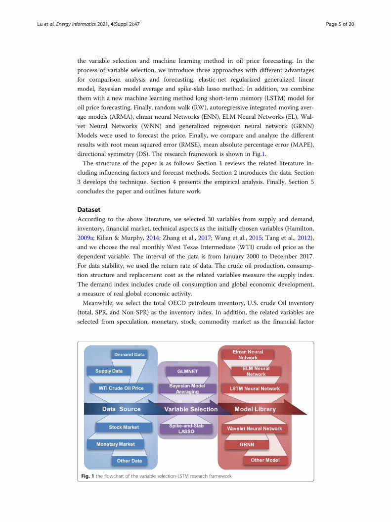
directional symmetry (DS). The research framework is shown in Fig.1.

The structure of the paper is as follows: Section 1 reviews the related literature in-

cluding influencing factors and forecast methods. Section 2 introduces the data. Section

3 develops the technique. Section 4 presents the empirical analysis. Finally, Section 5

concludes the paper and outlines future work.

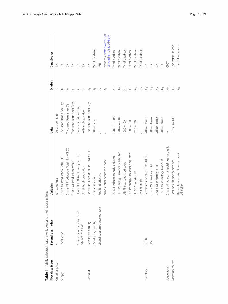
DatasetAccording to the above literature, we selected 30 variables from supply and demand,

inventory, financial market, technical aspects as the initially chosen variables (Hamilton,

2009a; Kilian & Murphy, 2014; Zhang et al., 2017; Wang et al., 2015; Tang et al., 2012),

and we choose the real monthly West Texas Intermediate (WTI) crude oil price as the

dependent variable. The interval of the data is from January 2000 to December 2017.

For data stability, we used the return rate of data. The crude oil production, consump-

tion structure and replacement cost as the related variables measure the supply index.

The demand index includes crude oil consumption and global economic development,

a measure of real global economic activity.

Meanwhile, we select the total OECD petroleum inventory, U.S. crude Oil inventory

(total, SPR, and Non-SPR) as the inventory index. In addition, the related variables are

selected from speculation, monetary, stock, commodity market as the financial factor

Fig. 1 the flowchart of the variable selection-LSTM research framework

Lu et al. Energy Informatics 2021, 4(Suppl 2):47 Page 5 of 20

index. Finally, we calculated the WTI-Brent spot price spread, actual value of the WTI

crack spread and Brent crack spread: actual value as the technical indicators. In Table 1,

we describe each variable and its corresponding data sources.

Theoretical backgroundAs the crude oil market is very complex and has various uncertain determinants, we must se-

lect the core influence factors first before establishing forecasting models. The main four vari-

able selection methods are significance test (forward and backward stepwise regression),

information criteria (AIC BIC), principal component factor analysis model, lasso regression,

ridge regression, and other punitive models (Castle et al., 2009). It is hard to tell which the

best is because each has its own strong and weak points. Thus, we introduce three different

methods to select core influence factors of crude oil price, which are elastic-net regularized

generalized linear Models (GlMNET), spike-slab lasso method (SSL) and Bayesian model

averaging (BMA). These three methods are effective variable selection methods and they are

all improvements on the existing mature models (LASSO, Ridge regression). Thus, we use

these new methods for variable selection (Zou & Hastie, 2005; Friedman et al., 2010).

Variable selection

The elastic-net regularized generalized linear Models (GLMNET)

Zou and Hastie (2005) (Zou & Hastie, 2005) proposed the elastic-net method for vari-

able selection, which is considered to be the best contraction method for handling mul-

ticollinearity and variable screening, and its loss precision is not too great. Their

simulation results showed that the elastic net outperformed the Lasso in terms of pre-

diction accuracy. Like the Lasso, the elastic net simultaneously does automatic variable

selection and continuous shrinkage, and it can select groups of correlated variables. On

the one hand, it achieves the purpose of ridge regression to select essential features; on

the other hand, it removes features that have little influence on dependent variables,

like Lasso regression, and achieves good results, especially when the sample size n is

smaller than the number of predictors. (The specific formula refers to (Zou & Hastie,

2005)) In this paper, we choose the Elastic-Net Regularization Linear Model

(GlMNET), which is a package that fits the Generalized Linear model by punishing

maximum likelihood (Friedman et al., 2010). The regularization path of the Lasso or

elastic net penalty is calculated on the value grid of the regularization parameter. The

algorithm is high-speed, can make full use of the sparsity of input matrix X, and is suit-

able for linear, logic, polynomial, poisson and Cox regression models. It can also be ap-

plied to multi-response linear regression. These algorithms can process vast datasets

and can make use of sparsity in the feature set.

minβ0;β

1N

XNi¼1

ωil yi; β0 þ βTxi� �þ λ 1−αð Þ βk k22=2þ α βk k1

� �

Wherein the values of the grid λ cover the entire range, l(yi, ηi) is the negative loga-

rithmic likelihood distribution of the contribution to the observed value i. For example,

it is 12 ðy−ηÞ2 for Gaussian. The elastic mesh penalty is controlled by α. (The specific

formula refer to Friedman et al. (2010)).

Lu et al. Energy Informatics 2021, 4(Suppl 2):47 Page 6 of 20

Table

1Initiallyselected

featurevariables

andtheirexplanations

Firstclassinde

xSe

cond

classindex

Variables

Units

Symbols

DataSo

urce

Crude

oilp

rice

/WTISpot

Price

Dollarspe

rBarrel

YEIA

Supp

lyProd

uctio

nCrude

OilProd

uctio

n,TotalO

PEC

Thou

sand

Barrelspe

rDay

X 1EIA

Crude

OilProd

uctio

n,TotalN

on-OPEC

Thou

sand

Barrelspe

rDay

X 2EIA

Crude

OilProd

uctio

n,World

Thou

sand

Barrelspe

rDay

X 3EIA

Con

sumptionstructureand

replacem

entcost

Hen

ryHub

NaturalGas

Spot

Price

Dollarspe

rMillionBtu

X 4EIA

U.S.tight

oilp

rodu

ction

millionbb

lper

day

X 5EIA

Dem

and

Develop

edcoun

try

Petroleum

Con

sumption,TotalO

ECD

Thou

sand

Barrelspe

rDay

X 6EIA

Develop

ingcoun

try

China

oilimpo

rtMilliontons

X 7Winddatabase

Globalecono

micde

velopm

ent

Fedfund

effective

/X 8

FRB

KilianGlobalecono

micinde

x/

X 9Web

site

ofhttp://www-203

person

al.umich.ed

u/lkilian/

USCPI

inde

x:season

allyadjusted

1982–84=100

X 10

Winddatabase

US:CPI:ene

rgy:season

allyadjusted

1982–84=100

X 11

Winddatabase

US:PPI:season

allyadjusted

1982

=100

X 12

Winddatabase

US:PPI:en

ergy:seasonally

adjusted

1982

=100

X 13

Winddatabase

EU28

Cou

ntries:PPI

2015

=100

X 14

Winddatabase

USPM

Iind

ex/

X 15

Winddatabase

Inventory

OEC

DPetroleum

inventory,TotalO

ECD

MillionBarrels

X 16

EIA

U.S.

Crude

Oilinventory,Total

MillionBarrels

X 17

EIA

Crude

Oilinventory,SPR

MillionBarrels

X 18

EIA

Crude

Oilinventory,Non

-SPR

MillionBarrels

X 19

EIA

Speculation

Crude

oiln

on-com

mercialne

tlong

ratio

%X 2

0CFC

T

Mon

etaryMarket

Realdo

llarinde

x:ge

neralized

197,303=100

X 21

Thefede

ralreserve

Theexchange

rate

ofeuro

against

USdo

llar

X 22

Thefede

ralreserve

Lu et al. Energy Informatics 2021, 4(Suppl 2):47 Page 7 of 20

Table

1Initiallyselected

featurevariables

andtheirexplanations

(Con

tinued)

Firstclassinde

xSe

cond

classindex

Variables

Units

Symbols

DataSo

urce

Stockmarket

S&P500inde

xX 2

3Winddatabase

Dow

Jone

sIndu

strialInd

exX 2

4Winddatabase

NASD

AQinde

xX 2

5Winddatabase

Com

mod

itymarket

COMEX:G

old:

Future

closingprice

Dollar/ou

nce

X 26

Winddatabase

LME:Cop

per:Future

closingprice

Dollar/ton

eX 2

7Winddatabase

Techno

logy

Indicators

pricespread

WTI-Brent

spot

pricespread

X 28

EIA

WTIcrackspread:actualvalue

X 29

EIA

Bren

tcrackspread:actualvalue

X 30

EIA

Lu et al. Energy Informatics 2021, 4(Suppl 2):47 Page 8 of 20

Bayesian model averaging

The basic idea of the Bayesian model averaging approach (BMA) can comprehend. Each

model is not fully accepted or not entirely negative (Leamer, 1978). The prior probability

of each model should be assumed firstly. The posterior probability can be gain by extract-

ing the dataset contains information as well as the reception of models to the dependent

variables. The excellence of the BMA approach is not only that it can sort the influence

factors according to their importance but also can calculate the posterior mean, standard

deviation and other indicators of the corresponding coefficients. With the help of the

Markov chain Monte Carlo method (MCMC), the weight distribution of the model ac-

cording to the prior information could be estimated (Godsill et al., 2001; Green, 1995).

The MCMC method can overcome the shortcoming of BIC, AIC and EM methods. (The

specific formula refer to (Leamer, 1978; Merlise, 1999; Raftery et al., 1997)).

It has the following three advantages: First, under different conditional probability

distributions, there is no need to change the algorithm. Second, the posterior distribu-

tion of the weight and variance of BMA is considered comprehensively. Third, it can

handle parameters with high BMA correlation.

Spike-slab lasso

Although model averaging can be considered a method of handling the variable selec-

tion and hypothesis testing task, only in a Bayesian context since model probabilities

are required. Recently, Ročková, V. and George, E. I. introduce a new class of self-

adaptive penalty functions that moving beyond the separable penalty framework based

on a fully Bayes spike-and-slab formulation (Ročková & George, 2018). Spike-slab Lasso

(SSL) can borrow strength across coordinates, adapt to ensemble sparsity information

and exert multiplicity adjustment by non-separable Bayes penalties. Meanwhile, it is

using a sequence of Laplace mixtures with an increasing spike penalty λ0, and keeping

λ1 fixed to a small constant. It is different from Lasso, which a sequence of single La-

place priors with an increasing penalty λ. Furthermore, it revisits deployed the EMVS

procedure (an efficient EM algorithm for Bayesian model exploration with a Gaussian

spike-and-slab mixture (Ročková & George, 2018)) for SSL priors, automatic variable

selection through thresholding, diminished bias in the estimation, and provably faster

convergence. (The specific formula refer to (Ročková & George, 2018)).

Long short-term memory network

Long short-term memory (LSTM) neural networks are a special kind of recurrent

neural network (RNN). LSTM was initially introduced by Hochreiter and Schmidhuber

(1997) (Hochreiter & Schmidhuber, 1997), and the primary objectives of LSTM were to

model long-term dependencies and determine the optimal time lag for time series is-

sues. In this subsection, the architecture of RNN and its LSTM for forecasting crude

oil prices are introduced. We start with the primary recurrent neural network and then

proceed to the LSTM neural network.

The RNN is a type of deep neural network architecture with a deep structure in the

temporal dimension. It has been widely used in time series modeling. A traditional

neural network assumes that all units of the input vectors are independent of each

other. As a result, the conventional neural network cannot make use of sequential

Lu et al. Energy Informatics 2021, 4(Suppl 2):47 Page 9 of 20

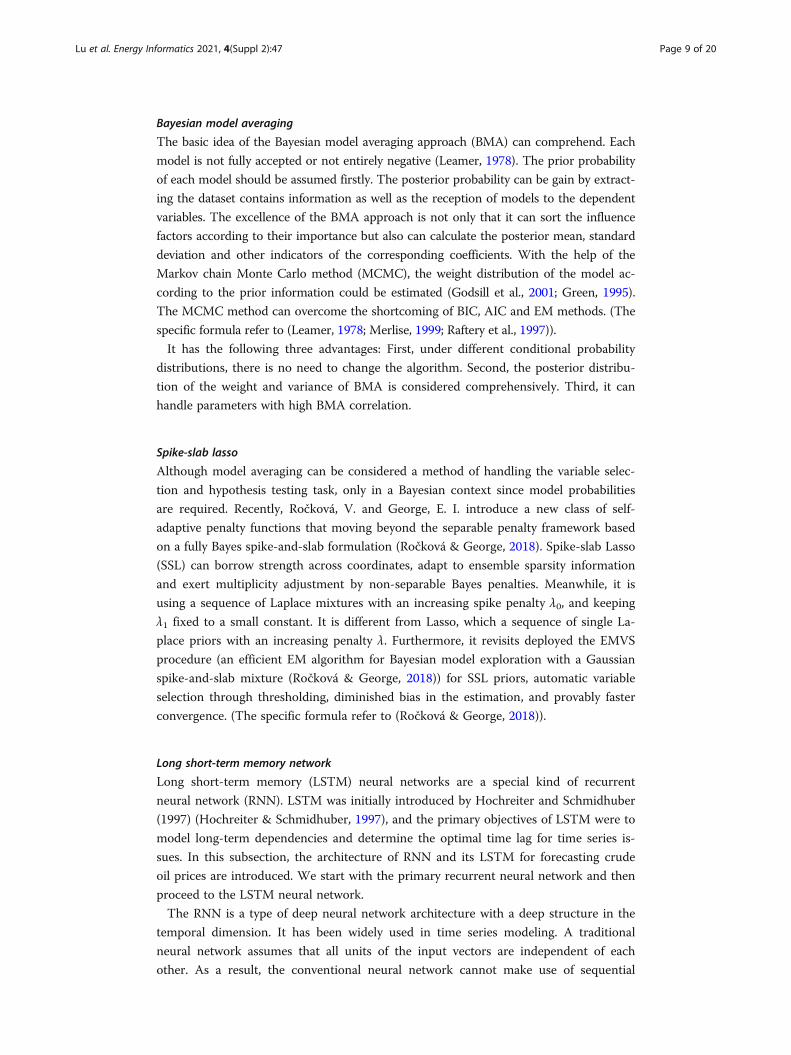
information. In contrast, the RNN model adds a hidden state generated by the sequen-

tial information of a time series, with the output dependent on the hidden state.

Figure 2 shows an RNN model being unfolded into a full network. The mathematical

symbols in Fig. 2 are as follows:

1. xt denotes the input vector at time t.

2. st denotes the hidden state at time t, which is determined relayed on the input vec-

tor xt and the previous hidden state. Then the hidden state st is determined as follows:

st ¼ f Uxt þWst−1ð Þ

Where f(·) is the activation function, it has many alternatives such as sigmoid

function and ReLU. The initial hidden state s0 is usually initialized to zero.

3. ot denotes the output vector at time t. It can be calculated by:

ot ¼ f Vstð Þ

4. U and V denote the weights of the hidden layer and the output layer respectively.

W denotes transition weights of the hidden state.

Although RNNs simulate time series data well, these are difficult to learn long-term

dependence because of the vanishing gradient issue. LSTM is an effective way to solve

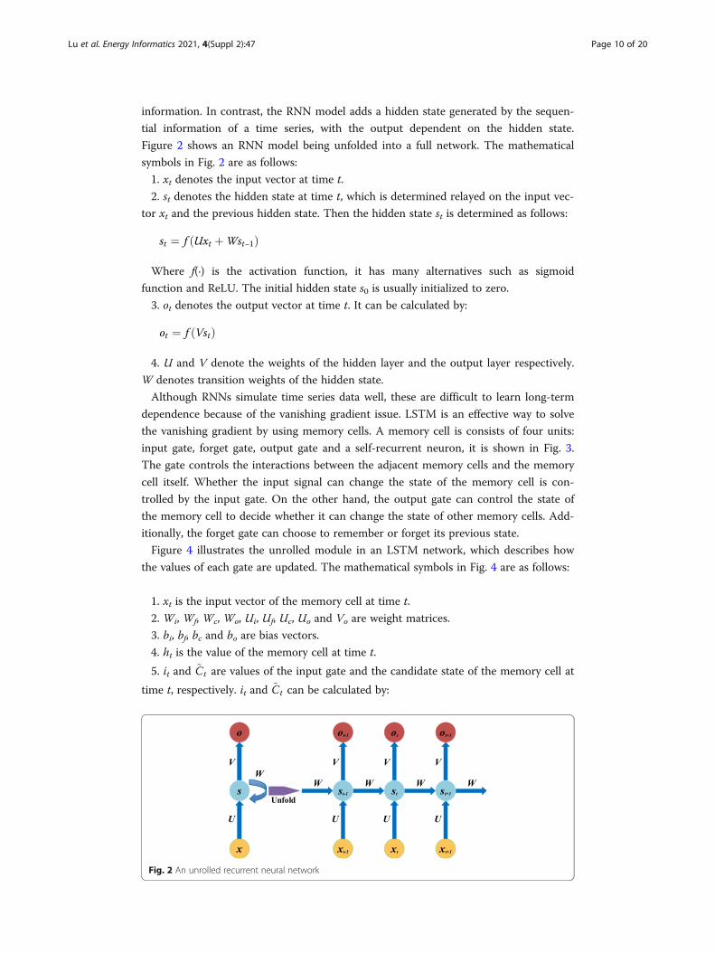
the vanishing gradient by using memory cells. A memory cell is consists of four units:

input gate, forget gate, output gate and a self-recurrent neuron, it is shown in Fig. 3.

The gate controls the interactions between the adjacent memory cells and the memory

cell itself. Whether the input signal can change the state of the memory cell is con-

trolled by the input gate. On the other hand, the output gate can control the state of

the memory cell to decide whether it can change the state of other memory cells. Add-

itionally, the forget gate can choose to remember or forget its previous state.

Figure 4 illustrates the unrolled module in an LSTM network, which describes how

the values of each gate are updated. The mathematical symbols in Fig. 4 are as follows:

1. xt is the input vector of the memory cell at time t.

2. Wi, Wf, Wc, Wo, Ui, Uf, Uc, Uo and Vo are weight matrices.

3. bi, bf, bc and bo are bias vectors.

4. ht is the value of the memory cell at time t.

5. it and ~Ct are values of the input gate and the candidate state of the memory cell at

time t, respectively. it and ~Ct can be calculated by:

Fig. 2 An unrolled recurrent neural network

Lu et al. Energy Informatics 2021, 4(Suppl 2):47 Page 10 of 20

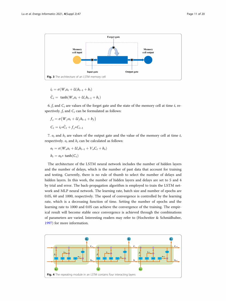
it ¼ σ Wixt þ Uiht−1 þ bið Þ~Ct ¼ tanh Wcxt þ Ucht−1 þ bcð Þ

6. ft and Ct are values of the forget gate and the state of the memory cell at time t, re-

spectively. ft and Ct can be formulated as follows:

f t ¼ σ W f xt þ U f ht−1 þ bf� �

Ct ¼ it�~Ct þ f t�Ct−1

7. ot and ht are values of the output gate and the value of the memory cell at time t,

respectively. ot and ht can be calculated as follows:

ot ¼ σ Woxt þ Uoht−1 þ VoCt þ boð Þht ¼ oh� tanh Ctð Þ

The architecture of the LSTM neural network includes the number of hidden layers

and the number of delays, which is the number of past data that account for training

and testing. Currently, there is no rule of thumb to select the number of delays and

hidden layers. In this work, the number of hidden layers and delays are set to 5 and 4

by trial and error. The back-propagation algorithm is employed to train the LSTM net-

work and MLP neural network. The learning rate, batch size and number of epochs are

0.05, 60 and 1000, respectively. The speed of convergence is controlled by the learning

rate, which is a decreasing function of time. Setting the number of epochs and the

learning rate to 1000 and 0.05 can achieve the convergence of the training. The empir-

ical result will become stable once convergence is achieved through the combinations

of parameters are varied. Interesting readers may refer to (Hochreiter & Schmidhuber,

1997) for more information.

Fig. 4 The repeating module in an LSTM contains four interacting layers

Fig. 3 The architecture of an LSTM memory cell

Lu et al. Energy Informatics 2021, 4(Suppl 2):47 Page 11 of 20

Empirical studyIn this section, we compare the variable selection-LSTM integrated learning approach

to the predictive performance of some benchmark models. First, section 4.1 analyzes

the core influencing factors for the screening of the three feature extraction methods,

and 4.2 describes the evaluation criteria and statistical tests to compare prediction ac-

curacy. Second, section 4.3 provides an input selection and reference model parameter

settings. Finally, Section 4.4 for the discussion.

Variable selection

We can see from Table 2, the elastic-net selects the most number (18 variables),

followed by the SSL method (11 variables), and the BMA method includes the least

number (8 variables). Meanwhile, the variable of the SSL method is a subset of the

BMA method, and the BMA method is a subset of the elastic-net. Non-OPEC produc-

tion, shale oil (tight oil) production, Fed Fund effective, Kilian Index, USA CPI, USA

PPI: Energy, Euro PPI, USA: PMI, OECD inventory, USA SPR inventory, USA Non-

SPR inventory, Crude oil non-commercial net long ratio, Real dollar index: generalized,

COMEX: Gold: Future closing price, LME: Copper: Future closing price, WTI-Brent

spot price spread, WTI crack spread: actual value and Brent crack spread: real value.

Firstly, we can see Non- OPEC production and tight oil production were selected from

the supply aspect. It suggested that with the reduction of OPEC production, the pro-

duction capacity of Non-OPEC countries is increasing gradually. In particular, the US

tight oil production has become an essential factor affecting the trend of oil prices in

recent years. According to the IEA report, the global oil production is expected to in-

crease by 6.4 million barrels to 107 million barrels by 2023. The US tight oil production

growth will account for 60 of the global growth. Meanwhile, in 2017, the US was the

world’s largest producer.

From the demand aspect, global economic development is still the main driver of

crude oil price. The USA PPI: energy, Euro PPI and USA: PMI factors are selected by

all three methods. Crude oil is an important raw material for industry, agriculture, and

transportation. It is also the main parent product of energy and chemical products in

the middle and lower reaches. Therefore, crude oil plays a critical role in the price of

domestic production and living materials. For example, when the oil price continued to

fall sharply, which is bound to lower the overall price level of the country. Moreover, it

will have a heavier negative effect on domestic currency fluctuations, which will shift

the currency situation from expansion to contraction.

From the inventory aspect, the OECD inventory, the USA SPR inventory and the

USA Non-SPR inventory are chosen into the elastic-net model. The inventor is an indi-

cator of the balance of the supply and demand for crude oil. Furthermore, the impact

of commercial inventory on oil prices is much more substantial. When the future price

Table 2 Selected key features by GLMNET, SSL and BMA method

Methods Selected feature ID

GLMNET X2, X5, X8, X9, X10, X13, X14, X15, X16, X18, X19, X20, X21, X26, X27, X28, X29, X30

Spike-slab Lasso X13, X14, X15, X20, X21, X27, X29, X30

Bayesian model averaging X13, X14, X15, X16, X18, X19, X20, X21, X27, X29, X30

Lu et al. Energy Informatics 2021, 4(Suppl 2):47 Page 12 of 20

is much higher than the spot price, the oil companies tend to increase the commercial

inventory, which stimulates the spot price to rise and reduces the price difference.

When the future price is lower than spot prices, oil companies tend to reduce their

commercial inventories, and spot prices fall, which will form a reasonable spread with

futures prices.

From the speculate aspect, there is a positive correlation between the non-

commercial net long ratio and oil price (Sanders et al., 2004). With the crude oil

market and the stock market relation gradually strengthened, hedging plays a more

important role in driving market trading (Coleman, 2012).

From the exchange rate market, the real dollar index: generalized was selected. The

dollar index is used to measure the degree of change in the dollar exchange rate against

a basket of currencies. If the dollar keeps falling, real revenues from oil products priced

in dollars will fall, which will lead to the crude price high.

Form the commodity market, the LME: Copper: Future closing price factor is picked

up. Copper has the function of resisting inflation, while the international crude oil price

is closely related to the inflation level. There is an interaction between them from the

long-term trend.

From the technical aspect, the WTI-Brent spread serves as an indicator of the tight-

ening in the crude oil market. As the spread widens, which suggests the global supply

and demand may be reached a tight equilibrium. The trend of price spread showed a

significant difference around 2015 because of the US shale oil revolution. US shale

production has surged substantially since 2014. However, due to the oil embargo, the

excess US crude oil could not be exported, resulting in a significant increase in US

Cushing crude oil inventories. The spread at this stage was mainly affected by the WTI

price, and the correlation between the price difference and the oil price trend was not

strong. After the United States lifted the ban on oil exports at the end of 2015, the cor-

relation between the price spread and the oil price trend increased significantly. After

the lifting of the oil export ban, the WTI oil price was no longer solely affected by the

internal supply and demand of the United States. During this period, Brent and WTI

oil prices were more consistent, resulting in a narrower spread. In addition, after 2015,

the consistency of them increased significantly.

In summary, the factors selected by all three models are USA PPI: Energy, Euro PPI,

USA: PMI (global economic development), Crude oil non-commercial net long ratio

(speculate factor), Real dollar index: generalized (exchange rate market), LME: Copper:

Future closing price (commodity market), WTI crack spread: actual value and Brent

crack spread: actual value (technology factor).

Evaluation criteria and statistic test

To compare the forecasting performance of our proposed approach with some other

benchmark models from level forecasting and directional forecasting, three main evalu-

ation criteria, i.e., root mean squared error (RMSE), mean absolute percentage error

(MAPE), directional symmetry (DS), which have been frequently used in recent years

(Chiroma et al., 2015; Mostafa & El-Masry, 2016; Yu et al., 2008b; Wang et al., 2017),

are selected to evaluate the in-sample and out-of-sample forecasting performance.

Three indicators are defined as follows:

Lu et al. Energy Informatics 2021, 4(Suppl 2):47 Page 13 of 20

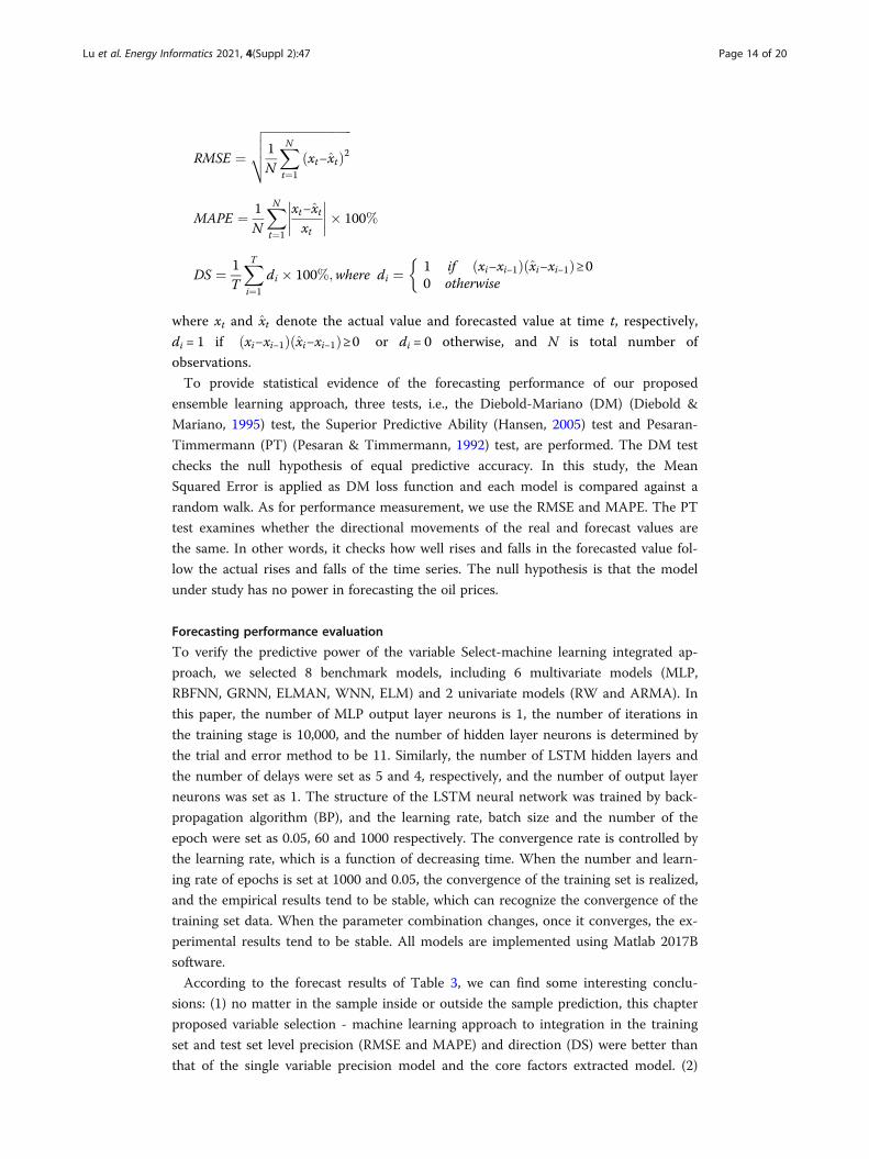
RMSE ¼ffiffiffiffiffiffiffiffiffiffiffiffiffiffiffiffiffiffiffiffiffiffiffiffiffiffiffiffiffi1N

XNt¼1

xt−x̂tð Þ2vuut

MAPE ¼ 1N

XNt¼1

xt−x̂txt

��������� 100%

DS ¼ 1T

XTi¼1

di � 100%;where di ¼ 1 if xi−xi−1ð Þ x̂i−xi−1ð Þ≥00 otherwise

�

where xt and x̂t denote the actual value and forecasted value at time t, respectively,

di = 1 if ðxi−xi−1Þðx̂i−xi−1Þ≥0 or di = 0 otherwise, and N is total number of

observations.

To provide statistical evidence of the forecasting performance of our proposed

ensemble learning approach, three tests, i.e., the Diebold-Mariano (DM) (Diebold &

Mariano, 1995) test, the Superior Predictive Ability (Hansen, 2005) test and Pesaran-

Timmermann (PT) (Pesaran & Timmermann, 1992) test, are performed. The DM test

checks the null hypothesis of equal predictive accuracy. In this study, the Mean

Squared Error is applied as DM loss function and each model is compared against a

random walk. As for performance measurement, we use the RMSE and MAPE. The PT

test examines whether the directional movements of the real and forecast values are

the same. In other words, it checks how well rises and falls in the forecasted value fol-

low the actual rises and falls of the time series. The null hypothesis is that the model

under study has no power in forecasting the oil prices.

Forecasting performance evaluation

To verify the predictive power of the variable Select-machine learning integrated ap-

proach, we selected 8 benchmark models, including 6 multivariate models (MLP,

RBFNN, GRNN, ELMAN, WNN, ELM) and 2 univariate models (RW and ARMA). In

this paper, the number of MLP output layer neurons is 1, the number of iterations in

the training stage is 10,000, and the number of hidden layer neurons is determined by

the trial and error method to be 11. Similarly, the number of LSTM hidden layers and

the number of delays were set as 5 and 4, respectively, and the number of output layer

neurons was set as 1. The structure of the LSTM neural network was trained by back-

propagation algorithm (BP), and the learning rate, batch size and the number of the

epoch were set as 0.05, 60 and 1000 respectively. The convergence rate is controlled by

the learning rate, which is a function of decreasing time. When the number and learn-

ing rate of epochs is set at 1000 and 0.05, the convergence of the training set is realized,

and the empirical results tend to be stable, which can recognize the convergence of the

training set data. When the parameter combination changes, once it converges, the ex-

perimental results tend to be stable. All models are implemented using Matlab 2017B

software.

According to the forecast results of Table 3, we can find some interesting conclu-

sions: (1) no matter in the sample inside or outside the sample prediction, this chapter

proposed variable selection - machine learning approach to integration in the training

set and test set level precision (RMSE and MAPE) and direction (DS) were better than

that of the single variable precision model and the core factors extracted model. (2)

Lu et al. Energy Informatics 2021, 4(Suppl 2):47 Page 14 of 20

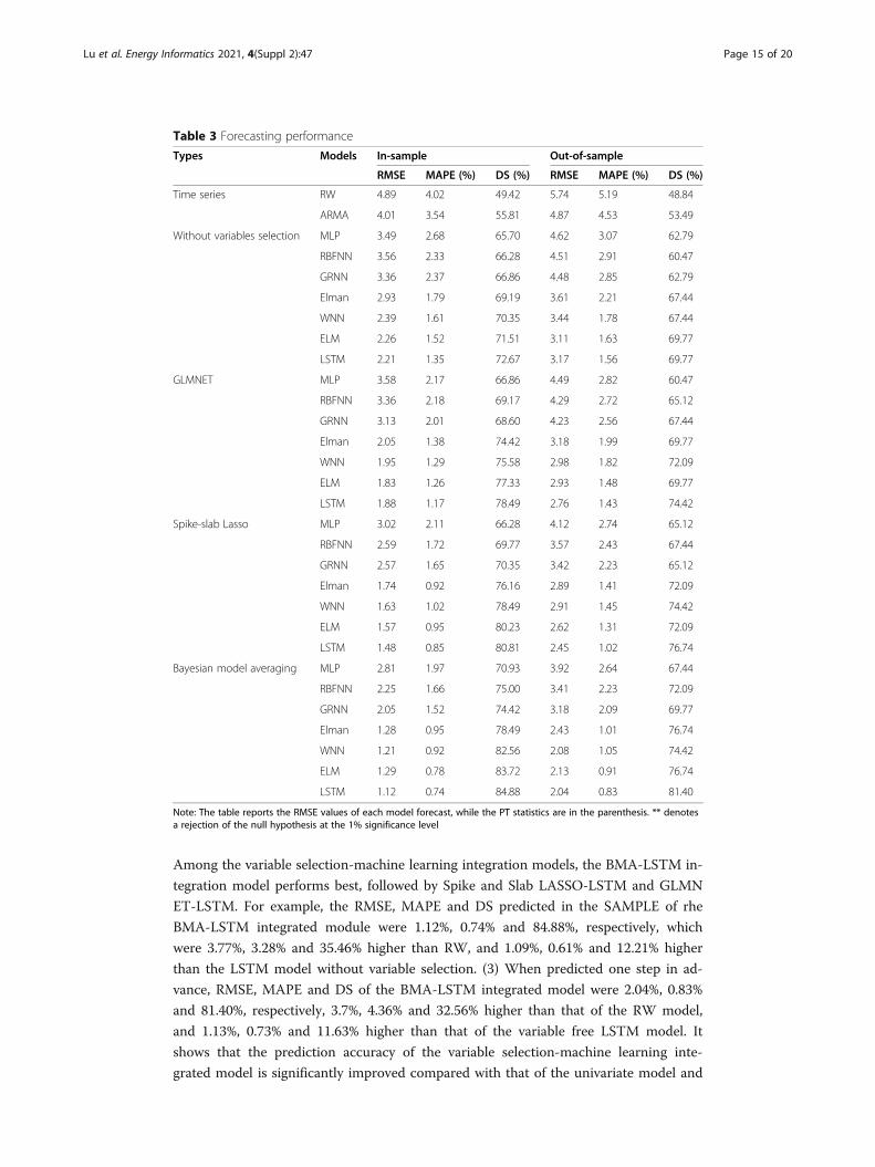
Among the variable selection-machine learning integration models, the BMA-LSTM in-

tegration model performs best, followed by Spike and Slab LASSO-LSTM and GLMN

ET-LSTM. For example, the RMSE, MAPE and DS predicted in the SAMPLE of rhe

BMA-LSTM integrated module were 1.12%, 0.74% and 84.88%, respectively, which

were 3.77%, 3.28% and 35.46% higher than RW, and 1.09%, 0.61% and 12.21% higher

than the LSTM model without variable selection. (3) When predicted one step in ad-

vance, RMSE, MAPE and DS of the BMA-LSTM integrated model were 2.04%, 0.83%

and 81.40%, respectively, 3.7%, 4.36% and 32.56% higher than that of the RW model,

and 1.13%, 0.73% and 11.63% higher than that of the variable free LSTM model. It

shows that the prediction accuracy of the variable selection-machine learning inte-

grated model is significantly improved compared with that of the univariate model and

Table 3 Forecasting performance

Types Models In-sample Out-of-sample

RMSE MAPE (%) DS (%) RMSE MAPE (%) DS (%)

Time series RW 4.89 4.02 49.42 5.74 5.19 48.84

ARMA 4.01 3.54 55.81 4.87 4.53 53.49

Without variables selection MLP 3.49 2.68 65.70 4.62 3.07 62.79

RBFNN 3.56 2.33 66.28 4.51 2.91 60.47

GRNN 3.36 2.37 66.86 4.48 2.85 62.79

Elman 2.93 1.79 69.19 3.61 2.21 67.44

WNN 2.39 1.61 70.35 3.44 1.78 67.44

ELM 2.26 1.52 71.51 3.11 1.63 69.77

LSTM 2.21 1.35 72.67 3.17 1.56 69.77

GLMNET MLP 3.58 2.17 66.86 4.49 2.82 60.47

RBFNN 3.36 2.18 69.17 4.29 2.72 65.12

GRNN 3.13 2.01 68.60 4.23 2.56 67.44

Elman 2.05 1.38 74.42 3.18 1.99 69.77

WNN 1.95 1.29 75.58 2.98 1.82 72.09

ELM 1.83 1.26 77.33 2.93 1.48 69.77

LSTM 1.88 1.17 78.49 2.76 1.43 74.42

Spike-slab Lasso MLP 3.02 2.11 66.28 4.12 2.74 65.12

RBFNN 2.59 1.72 69.77 3.57 2.43 67.44

GRNN 2.57 1.65 70.35 3.42 2.23 65.12

Elman 1.74 0.92 76.16 2.89 1.41 72.09

WNN 1.63 1.02 78.49 2.91 1.45 74.42

ELM 1.57 0.95 80.23 2.62 1.31 72.09

LSTM 1.48 0.85 80.81 2.45 1.02 76.74

Bayesian model averaging MLP 2.81 1.97 70.93 3.92 2.64 67.44

RBFNN 2.25 1.66 75.00 3.41 2.23 72.09

GRNN 2.05 1.52 74.42 3.18 2.09 69.77

Elman 1.28 0.95 78.49 2.43 1.01 76.74

WNN 1.21 0.92 82.56 2.08 1.05 74.42

ELM 1.29 0.78 83.72 2.13 0.91 76.74

LSTM 1.12 0.74 84.88 2.04 0.83 81.40

Note: The table reports the RMSE values of each model forecast, while the PT statistics are in the parenthesis. ** denotesa rejection of the null hypothesis at the 1% significance level

Lu et al. Energy Informatics 2021, 4(Suppl 2):47 Page 15 of 20

the univariate model. Secondly, the number of core variables selected by BMA is nei-

ther the most nor the least among the three variable selection models, indicating that

the number of core variables will also affect the prediction results.

Statistic tests

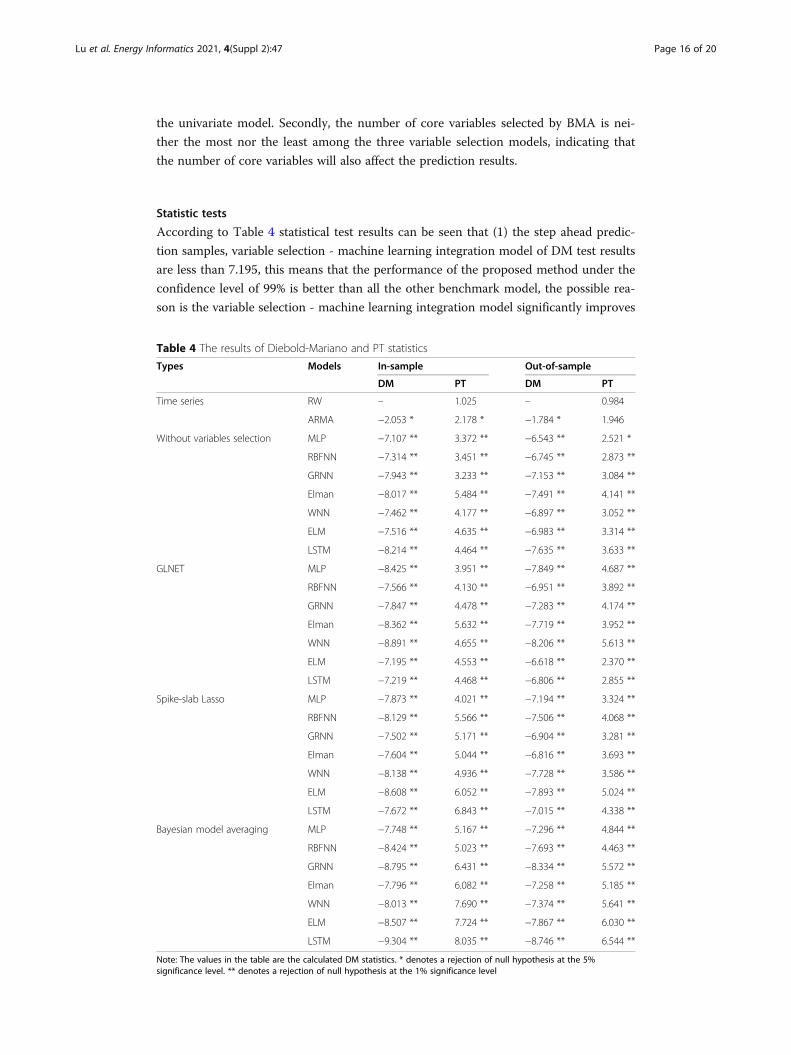
According to Table 4 statistical test results can be seen that (1) the step ahead predic-

tion samples, variable selection - machine learning integration model of DM test results

are less than 7.195, this means that the performance of the proposed method under the

confidence level of 99% is better than all the other benchmark model, the possible rea-

son is the variable selection - machine learning integration model significantly improves

Table 4 The results of Diebold-Mariano and PT statistics

Types Models In-sample Out-of-sample

DM PT DM PT

Time series RW – 1.025 – 0.984

ARMA −2.053 * 2.178 * −1.784 * 1.946

Without variables selection MLP −7.107 ** 3.372 ** −6.543 ** 2.521 *

RBFNN −7.314 ** 3.451 ** −6.745 ** 2.873 **

GRNN −7.943 ** 3.233 ** −7.153 ** 3.084 **

Elman −8.017 ** 5.484 ** −7.491 ** 4.141 **

WNN −7.462 ** 4.177 ** −6.897 ** 3.052 **

ELM −7.516 ** 4.635 ** −6.983 ** 3.314 **

LSTM −8.214 ** 4.464 ** −7.635 ** 3.633 **

GLNET MLP −8.425 ** 3.951 ** −7.849 ** 4.687 **

RBFNN −7.566 ** 4.130 ** −6.951 ** 3.892 **

GRNN −7.847 ** 4.478 ** −7.283 ** 4.174 **

Elman −8.362 ** 5.632 ** −7.719 ** 3.952 **

WNN −8.891 ** 4.655 ** −8.206 ** 5.613 **

ELM −7.195 ** 4.553 ** −6.618 ** 2.370 **

LSTM −7.219 ** 4.468 ** −6.806 ** 2.855 **

Spike-slab Lasso MLP −7.873 ** 4.021 ** −7.194 ** 3.324 **

RBFNN −8.129 ** 5.566 ** −7.506 ** 4.068 **

GRNN −7.502 ** 5.171 ** −6.904 ** 3.281 **

Elman −7.604 ** 5.044 ** −6.816 ** 3.693 **

WNN −8.138 ** 4.936 ** −7.728 ** 3.586 **

ELM −8.608 ** 6.052 ** −7.893 ** 5.024 **

LSTM −7.672 ** 6.843 ** −7.015 ** 4.338 **

Bayesian model averaging MLP −7.748 ** 5.167 ** −7.296 ** 4.844 **

RBFNN −8.424 ** 5.023 ** −7.693 ** 4.463 **

GRNN −8.795 ** 6.431 ** −8.334 ** 5.572 **

Elman −7.796 ** 6.082 ** −7.258 ** 5.185 **

WNN −8.013 ** 7.690 ** −7.374 ** 5.641 **

ELM −8.507 ** 7.724 ** −7.867 ** 6.030 **

LSTM −9.304 ** 8.035 ** −8.746 ** 6.544 **

Note: The values in the table are the calculated DM statistics. * denotes a rejection of null hypothesis at the 5%significance level. ** denotes a rejection of null hypothesis at the 1% significance level

Lu et al. Energy Informatics 2021, 4(Suppl 2):47 Page 16 of 20

the prediction performance of the model. (2) In the out-of-sample prediction 1 step in

advance, when the LR model is used as the test model, the DM test results of other test

models are far less than − 7.015, indicating that the predictive performance of the three

integrated methods and the other three single models is better than that of the machine

learning model without variable selection at the 99% confidence level. (3) samples

within 1 step ahead prediction and sample 1 step ahead prediction of the performance

of the three variables extraction method was compared, the BMA-LSTM integration

model to predict performance is the best, the next step is the Spike and slab LASSO-

LSTM and GLMNET-LSTM, suggesting that this chapter puts forward the integrated

research framework based on the variable selection-machine learning significantly im-

proves the performance of the integrated machine learning approach.

PT test results also give three interesting points: (1) In the one step forward in-

sample forecasting, the PT test results of the proposed variable selection-machine

learning integration approach are all rejected the movement direction of the actual in-

dependence assumption under 99% confidence level. This also means that the variable

selection-machine learning method is the best direction prediction performance and

also can be seen that the direction of the ARIMA predicts performance is the worst. (2)

In the out-of-sample one-step forecasting, the PT test value of the predicted results of

the integrated method is significantly greater than that of the single model, which

means that the direction prediction ability of the integrated method is better than that

of the single model, mainly because the variable selection-machine learning integration

idea significantly improves the direction prediction performance of the single model.

(3) In the prediction in and out of sample 1 step in advance, it can be seen from the

PT test results of variable Selection-machine learning integration method that the dir-

ection prediction accuracy of BMA-LSTM is the highest, followed by Spike-Slab Lasso-

LSTM, which is mainly attributed to the direction prediction ability of variable

Selection-machine learning method.

Conclusions and future workIn this paper, we proposed a variable selection and machine learning framework that

combines the variable selection (BMA) and forecasting method (LSTM) to forecast the

oil price and compared its forecasting performance with other primary and new vari-

able selection methods (elastic-net and spike and slab Lasso). Moreover, compared to

other popular benchmark forecast methods (RW, ARMA, MLP, RBFNN, GRNN,

ElMAN, WNN, ELM). Specifically, our contributions are as follow:

Introduce the variable selection before forecasting. In this process, we compare three

different methods and analyze core influencing factors based on the literature review

from supply and demand, global economic development, financial market, and technol-

ogy aspects. The results showed that the variable of the SSL method is a subset of the

BMA method, and the BMA method is a subset of the elastic-net.

Testing the performance of the proposed variable selection and machine learning

framework based on 3 variable selections and 8 individual forecasts. Comparing with

the 8 individual forecasts without variable selection, the combinations forecasting re-

duces the errors. The results showed that (1) the variable choice-machine learning inte-

gration method proposed in this chapter is superior to the univariate model and the

model without core factor extraction in both training set and test set level accuracy

Lu et al. Energy Informatics 2021, 4(Suppl 2):47 Page 17 of 20

(RMSE, MAPE) and direction symmetric (DS). (2) Among the variable selection-

machine learning integration models, The BMA-LSTM integration model performs

best, followed by Spike and Slab LASSO-LSTM and GLMNET-LSTM. It shows that

the prediction accuracy of the variable selection-machine learning integrated model is

significantly improved compared with that of the univariate model and the univariate

model. Secondly, the number of core variables selected by BMA is neither the most nor

the least among the three variable selection models, indicating that the number of core

variables will also affect the prediction results. (3) The statistical test results show that

the prediction of 1 step in advance in-sample and 1 step in advance in out of sample.

Compared with the prediction performance of the three variable extraction methods,

the directional prediction accuracy and horizontal prediction accuracy of the BMA-

LSTM integrated model are the best, followed by Spike and Slab-LASSO-LSTM and

GLMNET-LSTM. This indicates that the variable selection-based machine learning in-

tegrated research framework proposed in this chapter significantly improves the fore-

casting performance of oil prices. In future research, we may introduce more

independent variables with the help of internet search data, test our framework per-

formance. Moreover, investor sentiment can be quantified in this process. In addition,

different variable selection methods can be introduced more.

AbbreviationsANNs: artificial neural networks; ARMA: autoregressive moving average; ARIMA: autoregressive integrated movingaverage; BMA: Bayesian model averaging; DM: Diebold-Mariano; DS: directional symmetry; EMD: empirical modedecomposition; ENN: elman neural Networks; ETS: exponential smoothing; FNN: feed-forward neural network;GA: genetic algorithms; GARCH: generalized autoregressive conditional heteroskedastic model; GLMNET: elastic-netregularized generalized linear Model; GRNN: generalized regression neural network Models; LSTM: long short-termmemory; MIMO: multiple-input multiple-output; MAPE: mean absolute percentage error; MCMC: Markov chain MonteCarlo method; PT: Pesaran-Timmermann; RMSE: root mean squared error; RNN: recurrent neural network; RW: randomwalk; RWM: random walk model; SBM: slope-based method; SDAE: stacked denoising autoencoders model; SSL: Spike-slab Lasso; SVM: support vector machines; VAR: vector autoregression model; WNN: Walvet Neural Networks; WTI: WestTexas Intermediate

Supplementary InformationThe online version contains supplementary material available at https://doi.org/10.1186/s42162-021-00166-4.

Additional file 1. Neural networks training characteristics. Table A.1. Neural networks design and training characteristics

About this supplementThis article has been published as part of Energy Informatics Volume 4, Supplement 2 2021: Proceedings of theEnergy Informatics.Academy Conference Asia 2021. The full contents of the supplement are available at https://energyinformatics.springeropen.com/articles/supplements/volume-4-supplement-2.

Authors’ contributionsQ. L.: Data curation, Conceptualization, Methodology, Software, Writing - original draft, Funding acquisition; S. S.:Methodology, Writing - review& editing; H. D.: Writing - review& editing, Funding acquisition.; S. W.: Conceptualization,Supervision,Validation, Funding acquisition. All co-authors have read and approved the final manuscript.

FundingThis research is supported by the National Natural Science Foundation of China (71988101; 71874177 and72022019), China Postdoctoral Science Foundation (2020 M68719), and the University of Chinese Academy of Sciences.

Availability of data and materialsNot applicable.

Declarations

Ethics approval and consent to participateNot applicable.

Consent for publicationNot applicable.

Lu et al. Energy Informatics 2021, 4(Suppl 2):47 Page 18 of 20

Competing interestsThe authors declare that they have no competing interests.

Author details1Institute of Systems Science, Academy of Mathematics and Systems Science, Chinese Academy of Sciences, Beijing100190, China. 2 The School of Management Xi’an Jiaotong University Xi’an 710049 China . 3School ofEconomics and Management, University of Chinese Academy of Sciences, Beijing 100190, China.

Published: 24 September 2021

ReferencesBarsky RB, Kilian L (2001) Do we really know that oil caused the great stagflation? A monetary alternative. NBER Macroecon

Annu 16:137–183. https://doi.org/10.1086/654439Baumeister C, Kilian L, Zhou X (2013) Are product spreads useful for forecasting? An empirical evaluation of the verleger

hypothesis. Available at SSRN DP9572Castle JL, Qin X, Reed WR (2009) How to pick the best regression equation: a review and comparison of model selection

algorithms. Working Papers in Economics 32(5):979–986Chai J, Xing LM, Zhou XY, Zhang ZG, Li JX (2018) Forecasting the WTI crude oil price by a hybrid-refined method. Energy

Econ 71:114–127. https://doi.org/10.1016/j.eneco.2018.02.004Charles A, Darné O (2017) Forecasting crude-oil market volatility: further evidence with jumps. Energy Econ 67:508–519.

https://doi.org/10.1016/j.eneco.2017.09.002Chiroma H, Abdulkareem S, Herawan T (2015) Evolutionary neural network model for West Texas intermediate crude oil price

prediction. Appl Energy 142:266–273. https://doi.org/10.1016/j.apenergy.2014.12.045Cifarelli G, Paladino G (2010) Oil price dynamics and speculation: a multivariate financial approach. Energy Econ 32(2):363–

372. https://doi.org/10.1016/j.eneco.2009.08.014Coleman L (2012) Explaining crude oil prices using fundamental measures. Energy Policy 40:318–324. https://doi.org/10.1016/

j.enpol.2011.10.012Diebold FX, Mariano RS (1995) Comparing predictive accuracy. J Bus Econ Stat 20(1):134–144Doroodian K, Boyd R (2003) The linkage between oil price shocks and economic growth with inflation in the presence of

technological advances: a CGE model. Energy Policy 31(10):989–1006. https://doi.org/10.1016/S0301-4215(02)00141-6Drachal K (2016) Forecasting spot oil price in a dynamic model averaging framework-have the determinants changed over

time? Energy Econ 60:35–46. https://doi.org/10.1016/j.eneco.2016.09.020Drezga I, Rahman S (1998) Input variable selection for ANN-based short-term load forecasting. IEEE Transactions on Power

Systems Pwrs 13(4):1238–1244Friedman J, Hastie T, Tibshirani R (2010) Regularization paths for generalized linear models via coordinate descent. J Stat

Softw 33(1):1–22Godsill S, Doucet A, West M (2001) Maximum a posteriori sequence estimation using Monte Carlo particle filters. Ann Inst

Stat Math 53(1):82–96. https://doi.org/10.1023/A:1017968404964Green PJ (1995) Reversible jump Markov chain Monte Carlo computation and Bayesian model determination. Biometrika

82(4):711–732. https://doi.org/10.1093/biomet/82.4.711Hamilton JD (2009a) Understanding crude oil prices. Energy J 30(2):179–207Hamilton JD (2009b) Causes and consequences of the oil shock of 2007-08 (no. w15002). National Bureau of economic

researchHansen PR (2005) A test for superior predictive ability. J Bus Econ Stat 23(4):365–380. https://doi.org/10.1198/0735001

05000000063Hochreiter S, Schmidhuber J (1997) LSTM can solve hard long time lag problems. Adv Neural Inf Proces Syst:473–479Huang T, Fildes R, Soopramanien D (2014) The value of competitive information in forecasting FMCG retail product sales and

the variable selection problem. Eur J Oper Res 237(2):738–748. https://doi.org/10.1016/j.ejor.2014.02.022Ji Q, Fan Y (2016) Evolution of the world crude oil market integration: a graph theory analysis. Energy Econ 53:90–100.

https://doi.org/10.1016/j.eneco.2014.12.003Kilian L (2009) Not all oil price shocks are alike: disentangling demand and supply shocks in the crude oil market. Am Econ

Rev 99(3):1053–1069. https://doi.org/10.1257/aer.99.3.1053Kilian L (2010) Explaining fluctuations in gasoline prices: a joint model of the global crude oil market and the US retail

gasoline market. Energy J:87–112Kilian L (2017) How the tight oil boom has changed oil and gasoline markets Social Science Electronic Publishing Available

at SSRN No:6380Kilian L, Hicks B (2013) Did unexpectedly strong economic growth cause the oil price shock of 2003–2008? J Forecast 32(5):

385–394. https://doi.org/10.1002/for.2243Kilian L, Murphy DP (2014) The role of inventories and speculative trading in the global market for crude oil. J Appl Econ

29(3):454–478. https://doi.org/10.1002/jae.2322Korobilis D (2013) VAR forecasting using Bayesian variable selection. J Appl Econ 28(2):204–230. https://doi.org/10.1

002/jae.1271Leamer EE (1978) Specification searches. Wiley, New YorkMay RJ, Dandy GC, Maier HR, Nixon JB (2008) Application of partial mutual information variable selection to ANN forecasting

of water quality in water distribution systems. Environ Model Softw 23(10–11):1289–1299. https://doi.org/10.1016/j.envsoft.2008.03.008

Merlise A (1999) Bayesian model averaging and model search strategies. Bayesian Statistics 6:157Mostafa MM, El-Masry AA (2016) Oil price forecasting using gene expression programming and artificial neural networks.

Econ Model 54:40–53. https://doi.org/10.1016/j.econmod.2015.12.014Murat A, Tokat E (2009) Forecasting oil price movements with crack spread futures. Energy Econ 31(1):85–90. https://doi.org/1

0.1016/j.eneco.2008.07.008

Lu et al. Energy Informatics 2021, 4(Suppl 2):47 Page 19 of 20

Narayan PK, Narayan S, Zheng X (2010) Gold and oil futures markets: are markets efficient? Appl Energy 87(10):3299–3303.https://doi.org/10.1016/j.apenergy.2010.03.020

Özbek L, Özlale Ü (2010) Analysis of real oil prices via trend-cycle decomposition. Energy Policy 38(7):3676–3683. https://doi.org/10.1016/j.enpol.2010.02.045

Pesaran MH, Timmermann A (1992) A simple nonparametric test of predictive performance. J Bus Econ Stat 10(4):461–465Raftery AE, Madigan D, Hoeting JA (1997) Bayesian model averaging for linear regression models. J Am Stat Assoc 92(437):

179–191. https://doi.org/10.1080/01621459.1997.10473615Reboredo JC (2012) Modelling oil price and exchange rate co-movements. J Policy Model 34(3):419–440. https://doi.org/10.1

016/j.jpolmod.2011.10.005Ročková V, George EI (2018) The spike-and-slab lasso. J Am Stat Assoc 113(521):431–444. https://doi.org/10.1080/01621459.2

016.1260469Sadorsky P (1999) Oil price shocks and stock market activity. Energy Econ 21(5):449–469. https://doi.org/10.1016/S0140-9883

(99)00020-1Sanders DR, Boris K, Manfredo M (2004) Hedgers, funds, and small speculators in the energy futures markets: an analysis of

the CFTC's commitments of traders reports. Energy Econ 26(3):425–445. https://doi.org/10.1016/j.eneco.2004.04.010Sari R, Hammoudeh S, Soytas U (2010) Dynamics of oil price, precious metal prices, and exchange rate. Energy Econ 32(2):

351–362. https://doi.org/10.1016/j.eneco.2009.08.010Suganthi L, Samuel AA (2012) Energy models for demand forecasting-a review. Renew Sust Energ Rev 16(2):1223–1240.

https://doi.org/10.1016/j.rser.2011.08.014Sun S, Wei Y, Tsui KL, Wang S (2019) Forecasting tourist arrivals with machine learning and internet search index. Tour

Manag 70:1–10. https://doi.org/10.1016/j.tourman.2018.07.010Tang L, Yu L, Wang S, Li J, Wang S (2012) A novel hybrid ensemble learning paradigm for nuclear energy consumption

forecasting. Appl Energy 93:432–443. https://doi.org/10.1016/j.apenergy.2011.12.030Valgaev O, Kupzog F, Schmeck H (2020) Adequacy of neural networks for wide-scale day-ahead load forecasts on buildings

and distribution systems using smart meter data. Energy Informatics 3(1):1–17Wang J, Li X, Hong T, Wang S (2018) A semi-heterogeneous approach to combining crude oil price forecasts. Inf Sci

460:279–292Wang Q, Sun X (2017) Crude oil price: demand, supply, economic activity, economic policy uncertainty and wars–from the

perspective of structural equation modelling (SEM). Energy 133:483–490. https://doi.org/10.1016/j.energy.2017.05.147Wang Y, Liu L, Wu C (2017) Forecasting the real prices of crude oil using forecast combinations over time-varying parameter

models. Energy Econ 66:337–348. https://doi.org/10.1016/j.eneco.2017.07.007Wang Y, Wu C, Yang L (2015) Forecasting the real prices of crude oil: a dynamic model averaging approach. Available at

SSRN 2590195Wang Y, Wu C, Yang L (2016) Forecasting crude oil market volatility: a Markov switching multifractal volatility approach. Int J

Forecast 32(1):1–9. https://doi.org/10.1016/j.ijforecast.2015.02.006Xiong T, Bao Y, Hu Z (2013) Beyond one-step-ahead forecasting: evaluation of alternative multi-step-ahead forecasting

models for crude oil prices. Energy Econ 40(2):405–415. https://doi.org/10.1016/j.eneco.2013.07.028Yu L, Wang S, Lai KK (2008a) Forecasting crude oil price with an EMD-based neural network ensemble learning paradigm.

Energy Econ 30(5):2623–2635. https://doi.org/10.1016/j.eneco.2008.05.003Yu L, Wang S, Lai KK (2008b) Forecasting crude oil price with an EMD-based neural network ensemble learning paradigm.

Energy Econ 30(5):2623–2635. https://doi.org/10.1016/j.eneco.2008.05.003Yu L, Wang Z, Tang L (2015) A decomposition-ensemble model with data-characteristic-driven reconstruction for crude oil

price forecasting. Appl Energy 156:251–267. https://doi.org/10.1016/j.apenergy.2015.07.025Yu L, Zhao Y, Tang L, Yang Z (2019) Online big data-driven oil consumption forecasting with Google trends. Int J Forecast

35(1):213–223. https://doi.org/10.1016/j.ijforecast.2017.11.005Zhang JL, Zhang YJ, Zhang L (2015) A novel hybrid method for crude oil price forecasting. Energy Econ 49:649–659. https://

doi.org/10.1016/j.eneco.2015.02.018Zhang X, Lai KK, Wang SY (2008) A new approach for crude oil price analysis based on empirical mode decomposition.

Energy Econ 30(3):905–918. https://doi.org/10.1016/j.eneco.2007.02.012Zhang Y, Ma F, Wang Y (2019) Forecasting crude oil prices with a large set of predictors: can LASSO select powerful

predictors? J Empir Financ 54:97–117. https://doi.org/10.1016/j.jempfin.2019.08.007Zhang YJ (2013) Speculative trading and WTI crude oil futures price movement: an empirical analysis. Appl Energy 107:394–

402. https://doi.org/10.1016/j.apenergy.2013.02.060Zhang YJ, Chevallier J, Guesmi K (2017) “De-financialization” of commodities? Evidence from stock, crude oil and natural gas

markets. Energy Econ 68:228–239Zhang YJ, Wei YM (2011) The dynamic influence of advanced stock market risk on international crude oil returns: an

empirical analysis. Quantitative Finance 11(7):967–978. https://doi.org/10.1080/14697688.2010.538712Zhao Y, Li J, Yu L (2017) A deep learning ensemble approach for crude oil price forecasting. Energy Econ 66:9–16. https://doi.

org/10.1016/j.eneco.2017.05.023Zhu B, Han D, Wang P, Wu Z, Zhang T, Wei YM (2017) Forecasting carbon price using empirical mode decomposition and

evolutionary least squares support vector regression. Appl Energy 191:521–530. https://doi.org/10.1016/j.apenergy.2017.01.076

Zou H, Hastie T (2005) Regularization and variable selection via the elastic net. Journal of the Royal Statistical Society: Series B(Statistical Methodology) 67(2):301–320. https://doi.org/10.1111/j.1467-9868.2005.00503.x

Publisher’s NoteSpringer Nature remains neutral with regard to jurisdictional claims in published maps and institutional affiliations.

Lu et al. Energy Informatics 2021, 4(Suppl 2):47 Page 20 of 20