Atmos. Chem. Phys., 14, 9707–9725, 2014www.atmos-chem-phys.net/14/9707/2014/doi:10.5194/acp-14-9707-2014© Author(s) 2014. CC Attribution 3.0 License.

Analysing time-varying trends in stratospheric ozone time seriesusing the state space approach

M. Laine1, N. Latva-Pukkila1,2, and E. Kyrölä1

1Finnish Meteorological Institute, Earth Observation Unit, P.O. Box 503, 00101 Helsinki, Finland2Department of Mathematics and Statistics, P.O. Box (MaD), 40014 University of Jyväskylä, Jyväskylä, Finland

Correspondence to:M. Laine (marko.laine@fmi.fi)

Received: 11 July 2013 – Published in Atmos. Chem. Phys. Discuss.: 6 August 2013Revised: 4 August 2014 – Accepted: 14 August 2014 – Published: 16 September 2014

Abstract. We describe a hierarchical statistical state spacemodel for ozone profile time series. The time series are fromsatellite measurements by the Stratospheric Aerosol and GasExperiment (SAGE) II and the Global Ozone Monitoringby Occultation of Stars (GOMOS) instruments spanning theyears 1984–2011. Vertical ozone profiles were linearly inter-polated on an altitude grid with 1 km resolution covering 20–60 km. Monthly averages were calculated for each altitudelevel and 10◦ wide latitude bins between 60◦ S and 60◦ N.In the analysis, mean densities are studied separately for the25–35, 35–45, and 45–55 km layers. Model variables includethe ozone mean level, local trend, seasonal oscillations, andproxy variables for solar activity, the Quasi-Biennial Oscilla-tion (QBO), and the El Niño–Southern Oscillation (ENSO).

This is a companion paper toKyrölä et al.(2013), wherea piecewise linear model was used together with the sameproxies as in this work (excluding ENSO). The piecewiselinear trend was allowed to change at the beginning of 1997in all latitudes and altitudes. In the modelling of the presentpaper such an assumption is not needed as the linear trendis allowed to change continuously at each time step. Thisfreedom is also allowed for the seasonal oscillations whereasother regression coefficients are taken independent of time.According to our analyses, the slowly varying ozone back-ground shows roughly three general development patterns.A continuous decay for the whole period 1984–2011 is ev-ident in the southernmost latitude belt 50–60◦ S in all alti-tude regions and in 50–60◦ N in the lowest altitude region25–35 km. A second pattern, where a recovery after an ini-tial decay is followed by a further decay, is found at north-ern latitudes from the equator to 50◦ N in the lowest alti-tude region (25–35 km) and between 40◦ N and 60◦ N in the

35–45 km altitude region. Further ozone loss occurred after2007 in these regions. Everywhere else a decay is followedby a recovery. This pattern is shown at all altitudes and lati-tudes in the Southern Hemisphere (10–50◦ S) and in the 45–55 km layer in the Northern Hemisphere (from the equatorto 40◦ N). In the 45–55 km range the trend, measured as anaverage change in 10 years, has mostly turned from nega-tive to positive before the year 2000. In those regions wherethe “V” type of change of the trend is appropriate, the turn-ing point is around the years 1997–2001. To compare resultsfor the trend changes with the companion paper, we stud-ied the difference in trends between the years from 1984 to1997 and from 1997 to 2011. Overall, the two methods pro-duce very similar ozone recovery patterns with the maximumtrend change of 10 % in 35–45 km. The state space method(used in this paper) shows a somewhat faster recovery thanthe piecewise linear model. For the percent change of theozone density per decade the difference between the resultsis below three percentage units.

1 Introduction

Time series constructed from satellite remote sensing obser-vations provide important information about variability andtrends in atmospheric chemical composition. Many satel-lite time series provide global coverage of the measure-ment and some of the data sets run from the 1980s. Theanalysis of trends, both natural and anthropogenic, is com-plicated by natural variability and forcing affecting strato-spheric chemical compositions. In this study, the recov-ery of stratospheric ozone from the depletion caused by

Published by Copernicus Publications on behalf of the European Geosciences Union.

9708 M. Laine et al.: Time-varying trends in stratospheric ozone

chlorofluorocarbon (CFC) compounds is studied using a sta-tistical time series model.

Slow background changes in stratospheric ozone are eas-ily masked by both seasonal and irregular natural variabili-ties. Thus, the requirements are stringent for the stability ofozone observations. Self-calibrating occultation instrumentsare good candidates for such a task. The observations anal-ysed in this work consist of satellite measurements by theSAGE II and GOMOS instruments, operational during 1984–2005 and 2002–2012, respectively. The data set used herespans the years 1984–2011. Vertical ozone profiles were lin-early interpolated on an altitude grid with 1 km resolutioncovering 20–60 km. Monthly averages were calculated foreach altitude level and 10◦ wide latitude bins between 60◦ Sand 60◦ N. Combining the observations from different in-struments having different measurement principles is a chal-lenge.Kyrölä et al.(2013) explain the data set and its con-struction in more detail. Here the analysis is done with boththe original 1 km vertical spacing and by calculating meandensities over 10 km intervals.

There is a wealth of literature concerning the analysis ofatmospheric time series. A good reference to stratosphericozone time series regression analysis isSPARC(1998). A re-cent study that reviews the challenges and problems in trendanalysis of climatic time series was published byBates et al.(2012), and a general trend analysis reference isChandlerand Scott(2011). For state space and functional analysis ofatmospheric time series of similar type to that performedhere, seeLee and Berger(2003) andMeiring (2007).

This paper studies the feasibility and practical implemen-tation of a state space approach for atmospheric time se-ries analysis by defining a dynamic linear model (DLM) forstratospheric ozone time series. “Dynamic” means here thatthe regression coefficients can evolve in time. This makes itpossible to describe and analyse smooth changes in the aver-age background behaviour of ozone. Model variables includethe ozone mean level, local trend, seasonal oscillations, andproxy variables for solar activity, the Quasi-Biennial Oscilla-tion (QBO), and the El Niño–Southern Oscillation (ENSO).We do not claim novelty in the presented methods them-selves, but argue that they should be more extensively appliedin the analysis of climatic time series and provide a simpleframework for time series analyses that can be generalized tomore comprehensive studies. In this paper, we describe thenecessary steps for applying the methods.

A typical feature in atmospheric time series is that theyare not stationary but exhibit both slowly varying and abruptchanges in the distributional properties. These are causedby external forcing such as changes in the solar activity orvolcanic eruptions. Further, the data sampling is often non-uniform – there are data gaps, and the uncertainty of the ob-servations can vary. When observations are combined fromvarious sources there will be instrument and retrieval methodrelated biases. The differences in sampling lead to uncertain-ties, too. Straightforward linear regression analysis leaves the

model residuals correlated as not all variability can be ex-plained by a static linear structure. Usually this is compen-sated by allowing some correlation structure to the modelobservation error by using, e.g. an autoregressive model. Ifthe residual correlation is not accounted for, the model un-certainty analyses are misleading. A simple autoregressiveprocess can explain some of the unmodelled systematic vari-ations by correlated noise, again confusing the analyses. Inconclusion, much care in interpretation is needed for thosestandard classical statistical time series methods that requirestationarity, such as the ARIMA (autoregressive integratedmoving average) approach. The more general approach dis-cussed in this paper makes use of dynamic linear models andKalman filter type sequential estimation algorithms.

State space models, sometimes called hidden Markovmodels or structural time series models, are well known anddocumented in time series literature, e.g.Harvey (1990);Hamilton(1994); Migon et al.(2005). Modern computation-ally oriented references areDurbin and Koopman(2012) andPetris et al.(2009). Here, we review the basic properties rel-evant to the analysis of atmospheric ozone time series dataand explain the necessary steps to fit the model to monthlytime series observations and how to assess the uncertaintiesin the trend estimation.

The structure of this paper is the following. The data setsand the statistical model are described in Sect.2. Results ofthe statistical time series analyses are given in Sect.3 and thepaper ends with discussion and conclusions in Sect.4. Ap-pendixA contains mathematical and computational details.

2 Materials and methods

2.1 Ozone time series from satellite observations

We use a combination of two ozone data sets. The first con-sists of solar occultation measurements of ozone in the strato-sphere and lower mesosphere from the SAGE II instrument(Chu et al., 1989) operational during 1984–2005. The sec-ond is the GOMOS instrument (Bertaux et al., 2010) thatmeasured ozone in the stratosphere, mesosphere and lowerthermosphere during 2002–2012 using stellar occultations.The individual data sets have been homogenized to form acombined time series from 1984 to 2011. The stability of theSAGE II and GOMOS instruments, the construction of thecombined time series, data screening, bias correction, andother issues are discussed in more detail in the companionpaper byKyrölä et al.(2013). Four proxy time series are usedfor the solar flux, Quasi-Biennial Oscillations and ENSO.Except for ENSO, these proxies are the same as used in thecompanion paper. For ENSO we use the Multivariate ENSOIndex (MEI) from NOAA1.

1The MEI index is available fromhttp://www.esrl.noaa.gov/psd/enso/mei/.

Atmos. Chem. Phys., 14, 9707–9725, 2014 www.atmos-chem-phys.net/14/9707/2014/

M. Laine et al.: Time-varying trends in stratospheric ozone 9709

2.2 Statistical time series model

A general linear state space model with Gaussian errors canbe written with an observation equation and a state evolutionequation as

yt = Ftxt + vt , vt ∼ Np(0,Vt ), (1)

xt = Gtxt−1 + wt , wt ∼ Nq(0,Wt ), (2)

whereyt is a vector of lengthp containing the observationsandxt is a vector of lengthq of unobserved states of the sys-tem at timet . The state variables are used to describe the vari-ous components of the time series model, such as mean level,trend, seasonality and the effect of proxy variables. MatrixFt

is the observation operator mapping the unobserved states tothe observations and matrixGt is the model evolution oper-ator giving the dynamics of the states. In this basic formula-tion the uncertaintiesvt andwt are assumed to be Gaussian,with observation uncertainty covarianceVt and model errorcovarianceWt . Above,Np(0,Vt ) stands forp-dimensionalGaussian distributions, with vector of zeros as mean andVt

as thep×p covariance matrix. The time indext will go from1 toN , the length of the time series to be analysed. In the fol-lowing, the matrices defining the model will mostly be timeinvariant, i.e.Gt = G, etc., and we will usually drop the timesubscript, still retaining it in general formulas that are notspecific to this particular time series application.

In this work, we use a DLM to explain variability in theozone time series with four components: smooth locally lin-ear trend, seasonal effect, effect of forcing via proxy vari-ables, and noise that is allowed to have autoregressive cor-relation. All components are built using the state space ap-proach.

To describe the trend we start with a simple local leveland locally linear trend model that has two hidden statesxt = [µt ,αt ]

T , whereµt is the mean level andαt is thechange in the level from timet to time t + 1. In addition weneed stochastic terms for the observational error and for theallowed change in the dynamics of the trend and the level.These are defined by Gaussian “ε” terms below. The systemcan be written by equations

yt = µt + εobs, εobs∼ N(0,σ 2obs(t)), (3)

µt = µt−1 + αt−1 + εlevel, εlevel ∼ N(0,σ 2level), (4)

αt = αt−1 + εtrend, εtrend∼ N(0,σ 2trend). (5)

In terms of the state space equations (1) and (2) this becomes

Gtrend=

[1 10 1

], Ftrend=

[1 0

],

Wtrend=

[σ 2

level 00 σ 2

trend

], Vt =

[σ 2

obs(t)

]. (6)

Depending on the choice of variancesσ 2level andσ 2

trend, thiswill define a smoothly varying background level of the dataseries that is used to infer changes in atmospheric ozone.

Most atmospheric series exhibit seasonal variability. Theseasonality can be modelled using harmonic functions. If thenumber of cyclic components iss, the full seasonal modelhass/2 harmonics. For thekth harmony, withk = 1, . . . , s/2,we need to add two state variables. With monthly data wehaves = 12 and the corresponding blocks of the model andobservation matrices are

Gseas(k) =

[cos(k2π/12) sin(k2π/12)

−sin(k2π/12) cos(k2π/12)

],

Fseas(k) =[1 0

]andWseas(k) =

[σ 2

seas(k) 00 σ 2

seas(k)

]. (7)

Here the state equation matrices are independent of timeindex t and we have used subscriptk to stand for theharmonic component. The rationale behindGseas(k) isthat if we know the harmonicut,k = ak cos(k2π/12t) +

bk sin(k2π/12t) and, as an auxiliary state, its conjugateu∗

t,k = −ak sin(k2π/12t)+bk cos(k2π/12t), with some con-stantsak andbk, we can update the state with[ut+1,k

u∗

t+1,k

]= Gseas(k)

[ut,k

u∗

t,k

], (8)

whereGseas(k) is defined in Eq. (7) and does not depend ontime t (e.g.Petris et al., 2009, Sect. 3.2.3). In our case theseasonality can be adequately explained by two harmonics,e.g. by yearly and half-a-year variation (k = 1 andk = 2),which will increase the number of hidden states to be esti-mated by four. In addition we need to define the error co-variance matrixWseasfor the allowed time-wise variabilityin the seasonal components. We note that there is no need fora separate seasonal observation error matrixVseas, asVt isused only in the observation equation (1), not in the modelequation (2) where the seasonal cycle is defined.

In the previous definitions, the state operatorG, the ob-servation operatorF and the model error covarianceW havebeen time invariant. The observation uncertainty covarianceVt defined in Eq. (6) is, in our case, time dependent andit will contain the known observation uncertainties. The in-clusion of auxiliary proxy variables is done by augmentingthe observation matrixFt , making it time dependent. In thefollowing, the stratospheric ozone analysis will utilize fourproxy time series explaining parts of the natural variability:one for the solar flux, two proxy variables for QBO, and onefor ENSO. This is achieved by adding the following compo-nents into the system matrices:

www.atmos-chem-phys.net/14/9707/2014/ Atmos. Chem. Phys., 14, 9707–9725, 2014

9710 M. Laine et al.: Time-varying trends in stratospheric ozone

Gproxy =

1 0 0 00 1 0 00 0 1 00 0 0 1

,

Fproxy(t) =[z1,t z2,t z3,t z4,t

]and

Wproxy =

σ 2

z1 0 0 00 σ 2

z2 0 00 0 σ 2

z3 00 0 0 σ 2

z4

, (9)

wherez1,t , z2,t , z3,t andz4,t contain the values of the fourproxy series at timet . With positive error variancesσ 2

zi this isan extension of linear regression analysis into one with time-varying coefficients. In our analysis, for simplicity, we set allthe elements of the model error covariance matrixWproxy tozero to obtain time-invariant regression coefficients for theproxy variables.

To allow autocorrelation in the residuals we use a first-order autoregressive model (AR(1)). This is similar to theCochrane–Orcutt correction in classical multiple regression(see e.g.Hamilton, 1994) used byKyrölä et al.(2013). How-ever, in the DLM approach we can estimate the autocorre-lation coefficient and the extra variance term together withthe other model parameters, not by a separate iteration, asneeded, e.g. by the Cochrane–Orcutt method. A first-orderautoregressive model for a state componentηt can be writ-ten asηt = ρηt−1 + εAR, with εAR ∼ N(0,σ 2

AR), whereρ isthe AR coefficient andσ 2

AR is usually called the innovationvariance in classical time series literature. In DLM form, wesimply have

GAR =[ρ],FAR =

[1], andWAR =

[σ 2

AR

], (10)

and bothρ andσ 2AR can be estimated from the observations.

The next step in DLM model construction is the combina-tion of the selected individual model components into largermodel evolution and observation equations. For the modelevolution matrixG and the observation operatorFt we have

G =

Gtrend 0 0 0 0

0 Gseas(1) 0 0 00 0 Gseas(2) 0 00 0 0 Gproxy 00 0 0 0 GAR

,

Ft =[Ftrend Fseas(1) Fseas(2) Fproxy(t) FAR

], (11)

In our analyses, the state vectorxt has a total of 11 compo-nents:

xt =[µt αt ut,1 u∗

t,1 ut,2 u∗

t,2

β1 β2 β3 β4 ηt ]T , (12)

whereµt is the local mean,αt is the local trend, i.e. the localchange of the mean,ut,k andu∗

t,k are the states representing

the two seasonal harmonics, theβ are the regression coef-ficients for the four proxy variables, andηt is an extra statefor the autoregressive component that “remembers” the valueof the observation from the previous time step. In this study,the regression coefficients (β) are assumed not to depend ontime t . The full model error covariance matrixW is a diago-nal matrix with the corresponding variances at the diagonal,

diag(W) =

[0 σ 2

trend σ 2seas σ 2

seas σ 2seas σ 2

seas

0 0 0 0 σ 2AR

], (13)

where the local level variance and the proxy regression coef-ficient variances have been set to zero and the four seasonalvariances set to be all equal, to correspond to the simplifi-cation assumed in the analyses. Lastly, as already stated, theobservation error covariance matrixVt , will be a 1×1 matrixand equals the known observation uncertainty:Vt = σ 2

obs(t).Next, the analysis will proceed to the specification of thevariance parameters and other parameters in the model for-mulation (e.g. the AR coefficientρ above), and to the esti-mation of the model states by state space methods.

2.3 Model parameter estimation

We have two kinds of unknowns, the model state variablesxt , one vector for each timet , and the auxiliary parametersthat define the model error covariance matrixW and the sys-tem evolution matrixG. At first sight, this might seem to bea vastly underdetermined system, as we have several modelparameters for each single observation. However, by the se-quential nature of the equations, we can estimate the statesby standard recursive Kalman filter formulas.

Implicitly assumed in the state space equations (1) and(2) is that the state at timet is statistically conditionallyindependent of the history given the previous state at timet − 1. When the model equation matrices are known, thisMarkov property allows sequential estimation of the statesgiven the observations by famous Kalman formulas (see e.g.Rodgers, 2000). We can use a Kalman filter for one-step-ahead prediction of the state and a Kalman smoother for themarginal probability distribution of the state at timet giventhe whole time series of all observations (t = 1, . . . ,N ).Marginal means that the uncertainty of the states at all othertimes thant has been accounted for. In time series applica-tions, the Kalman filter output can be used to calculate themodel likelihood function, needed in the estimation of theauxiliary parameters, and the Kalman smoother provides anefficient algorithm to estimate the model states and to de-compose time series into parts given by the model formula-tion. Thus, this high-dimensional problem is computationallynot much more intensive than a classical static multiple lin-ear regression analysis. Furthermore, in the linear Gaussiancase, the probability distributions provided by the Kalmanformulas are exact, not approximations. Non-linear modelscan be approached by linearization of the state equations, and

Atmos. Chem. Phys., 14, 9707–9725, 2014 www.atmos-chem-phys.net/14/9707/2014/

M. Laine et al.: Time-varying trends in stratospheric ozone 9711

non-Gaussian error models by, e.g. particle filter algorithms(Doucet et al., 2001). More details on the DLM computationscan be found in AppendixA.

Next, we consider the model error covariance matrixW.If we set all model error variances to zero it will change theDLM model into an ordinary, non-dynamic, multiple linearregression model. By using non-zero variances we can fita smoothly varying mean level, and the smoothness can becontrolled by the size of the variances. A simplification donehere is that we assumeW to be diagonal, and even some ofthe diagonal elements are set to zero. In our case non-zeroelements are the variability of the trend,σ 2

trend, and the vari-ances of seasonal variation,σ 2

seas(k), i.e. we will set the vari-ance of the level and the four proxy variables to zero. Ourmotivation for excluding dynamic variation from the proxiesis to use an as simple as possible dynamic model that wouldhave similar properties as the piecewise linear model in thecompanion paper. By studying dynamic changes in the trendand seasonal variation we will then either validate the staticlinear approach or show that it is not appropriate.

A common procedure to estimate the elements of themodel error matrixW is based on the maximum likeli-hood method using the likelihood function provided by theKalman filter. After the estimation, the obtained values couldbe plugged into the system equations as known constants.However, this plug-in method neglects the uncertainty in theestimates. Instead, we will use an alternative method basedon Bayesian analysis (Gamerman, 2006; Petris et al., 2009;Särkkä, 2013) and outline it shortly below in Sect.2.4.

2.4 Markov chain Monte Carlo analysis for modelparameters

The Markov chain Monte Carlo (MCMC) method providesan algorithm to draw samples from the Bayesian posterioruncertainty distribution of model parameters given the likeli-hood function and the prior distribution (Gamerman, 2006).As the Kalman filter likelihood provides the likelihood ofthe auxiliary model parameters, marginalized over the un-known model states, we can use it to draw samples from themarginal posterior distribution of these parameters. We willuse an adaptive Metropolis algorithm ofHaario et al.(2006)for the three unknown variance parameters (σtrend, σseas, σAR)in the matrixW in Eq. (13) as well as for the autoregressiveparameterρ in the system evolution matrixG (Eq.10). Afterobtaining this sample from the posterior distribution, we usesampled parameter values, one by one, to simulate realiza-tions of the model statesx1:N using the Kalman simulationsmoother (e.g.Petris et al., 2009). This allows us to accountfor both the parameter and the model state uncertainties in thetrend analysis. Again, more computational details are givenin AppendixA.

For Bayesian analysis of the unknown model parameters,prior distributions for the parameters must be specified. Wewant the variances in the matrixW to reflect our prior knowl-

edge on the assumed variability in the processes captured bythe observations. As noted byGamerman(2006, Sect. 2.5.),dynamic linear models offer intuitive means of providingqualitative prior information in the form of the model equa-tions and quantitative information by prior distributions onvariance parameters. By the estimation procedure we aim atfinding variance parameters that are consistent with the givenobservation uncertainty, i.e. the model can predict the obser-vations within their accuracy. This means that the scaled pre-diction residuals that are used defining the likelihood func-tion should behave like an independent Gaussian randomvariable. We can assess these assumptions by different resid-ual analysis diagnostics.

As we are effectively looking for slowly varying trendsin the data, we will set prior constraints to variance param-eters to reflect this. For example, we might assume that thechange within a month in the background level is on the av-erage some percentage of the overall time series mean. Theestimation procedure will then divide the observed variabil-ity into model components (level, trend, seasonality) in pro-portions that reflect the prior choices. The standard modeldiagnostic tools, such as autocorrelation analysis and normalprobability plots, can be used to reveal possible discrepan-cies in the model assumptions that have to be considered. Asthe model residuals are calculated from one-step predictions,the diagnostics will reveal both over-fit and a lack of fit.

The model error covarianceW (Eq. 13) is time invari-ant, with nonzero diagonal terms for the trend parameter, acommon value for the four parameters defining the variabil-ity in the seasonal components, and one value for the vari-ance defining the autoregressive component. For MCMC es-timation of the variance parameters, we use log-normal priordistributions for the corresponding standard deviations. Themotivation for this is that the standard deviations are posi-tive by definition so logarithmic scale is natural and com-monly used and it allows prior specification in meaningfulunits. If a random variablex follows a log-normal distri-bution logN(µ,σ 2), then log(x) follows the standard Gaus-sian distributionN(µ,σ 2). Because of this transformation,it is more intuitive to work with a log mean parameter, asin logN(log(µ),σ 2), whereµ is now the approximate meanof the untransformedx and the scale parameter of the log-normal distributionσ can be interpreted as an approxima-tion of the relative standard deviation of the original variablein question. The prior distribution for the standard deviationof the monthly level changeσtrend was set to be log-normalwith the log mean equal to 1/12 % of the average level ofthe ozone observations and having scale parameter 1. Thisscale corresponds to a relatively wide (130 % SD)2 prior un-certainty forσtrend. All the σ parameters describe allowed

2This can be derived from the fact that ifx ∼ logN(µ,σ2) thenits mean and variance areE(x) = exp(µ + 1/2σ2) and D(x) =

exp(2µ)exp(σ2)(exp(σ2)−1), see e.g. Wikipedia entry for the log-normal distribution.

www.atmos-chem-phys.net/14/9707/2014/ Atmos. Chem. Phys., 14, 9707–9725, 2014

9712 M. Laine et al.: Time-varying trends in stratospheric ozone

0 0.005 0.01 0.015

σtrend

0 0.005 0.01 0.015

σseas

0.2 0.25 0.3 0.35

σAR

0.2 0.4 0.6 0.8 1

ρAR

mcmc chain

prior

Fig. 1. Results of MCMC analysis for the four unknown model parameter: trend change standard deviation

σtrend, seasonal change standard deviation σtrend, autoregressive standard deviation σAR, and the autoregres-

sive coefficient ρ. The histograms are estimates of the corresponding marginal posterior probability densities

obtained by MCMC analysis with 10 000 simulation steps. The parameters are for 40◦ N–50◦ N, 35–45 km as

in Fig. 2. The prior probability densities given by dashed lines are log-normal for the standard deviations and

truncated Gaussian for the AR parameter ρ. For the analysis the ozone observation have been scaled by their

observed standard deviation. This means that the values given in the x axes are also scaled so that the overall

variance of the ozone observations is one.

22

Figure 1. Results of MCMC analysis for the four unknown modelparameters: trend change standard deviationσtrend, seasonal changestandard deviationσtrend, autoregressive standard deviationσARand the autoregressive coefficientρ. The histograms are estimates ofthe corresponding marginal posterior probability densities obtainedby MCMC analysis with 10 000 simulation steps. The parametersare for 40–50◦ N, 35–45 km as in Fig.2. The prior probability densi-ties given by dashed lines are log-normal for the standard deviationsand truncated Gaussian for the AR parameterρ. For the analysis theozone observations have been scaled by their observed standard de-viation. This means that the values given on thex axes are alsoscaled so that the overall variance of the ozone observations is one.

change in one time interval of the model and data (month),i.e. the unit forσtrend is 1cm−3. For the seasonal standarddeviation,σseas, we set the log mean parameter to 1 % ofthe overall variability in the observed ozone values and thescale parameter to 2 (corresponding to 730 % SD). For thestandard deviation of the AR(1) component (Eq.10), we use30 % of the observed variability for the log mean and simi-larly 2 for the scale. For the autoregressive coefficientρ theprior was GaussianN(0.45,0.5) truncated to be in the inter-val [0,1]. Table1 collects the prior specifications. The re-sults for the trend analyses or the estimated parameter valuesthemselves are not sensitive to the chosen priors. The MCMCfor each separate fit was run using 10 000 simulation steps,and the resulted parameter samples (chains in MCMC termi-nology) were checked for convergence of the algorithm. Thehistograms of the marginal posterior samples of the parame-ters with the prior probability density functions overlaid areshown in Fig.1 for one zonal band and altitude region. Theprior for the trend variability would allow the trend to change

1985 1990 1995 2000 2005 20104.5

5

5.5

6

6.5

7

7.5x 10

11 40° N − 50° N, 35−45 km

time

aver

age

ozon

e [1

/cm

3 ]

GOMOS

SAGE II

1985 1990 1995 2000 2005 2010−0.7

−0.6

−0.5

−0.4

−0.3

−0.2

−0.1

0

0.1

0.210 year trend

% c

hang

e / y

ear

time

0 5 10 15 20−0.5

0

0.5

1

lag

acf

Estimated autocorrelation function of the DLM residuals

−3 −2 −1 0 1 2 3−4

−2

0

2

4

Theoretical Quantiles

Empi

rical

Qua

ntile

s

Normal probability plot for the residuals

Figure 2. DLM fit for average ozone at 40–50◦ N, 35–45 km. In theupper panel the dots are the observations used in the analysis, thesolid line following the observations is the DLM fit obtained by aKalman filter. The smooth solid line is the background level compo-nent of the model with 95 % probability envelope. The beginning ofGOMOS observations as well as the end of SAGE II are shown byred vertical lines. In the lower left panel an analysis of the 10-yeartrend is performed, showing the mean estimated trend and its 95 %probability envelope. The lower right panel shows model diagnos-tic analyses on the residuals by an estimated autocorrelation func-tion (ACF) and by a normal probability plot. In the autocorrelationfunction plot, dashed horizontal lines correspond to the approxima-tive region where the coefficients do not significantly (95 %) deviatefrom zero. The unit of lag is months.

Atmos. Chem. Phys., 14, 9707–9725, 2014 www.atmos-chem-phys.net/14/9707/2014/

M. Laine et al.: Time-varying trends in stratospheric ozone 9713

1

1.5

2

2.5

3x 10

12 alt: 20 km, lat: 10° S − 0° S

ozo

ne

[1

/cm

3]

GOMOS

SAGE II

−5

0

5scaled prediction residuals

GOMOS

SAGE II

−10

0

10seasonal

GOMOS

SAGE II

[%]

−10

0

10 GOMOS

SAGE II

QBOs

[%]

−202

solar

[%]

GOMOS

SAGE II

1985 1990 1995 2000 2005 2010−10−5

05

ENSO

[%]

GOMOS

SAGE II

Fig. 3. Some of the DLM model components for 10◦ S–0◦ S, 20 km. The first panel has the observations

and the level components as in Fig. 2. In addition, the piecewise linear regression model used by Kyrola

et al. (2013) is drawn with a solid green line. The second panel downwards shows model residuals, scaled by

the estimated residual standard deviation, i.e. the variability in the y axis direction should be approximately

standard Gaussian N (0,1). The other panels show means and 95% probability envelopes (the grey shading)

of the DLM components related to seasonality and to the proxy variables, solar, Quasi-Biennial Oscillation,

and ENSO, i.e. the original proxy variables multiplied by the estimated regression coefficients. For the proxy

variables, the y axis scaling is the percentage of the total ozone variability, i.e. the ozone observations were

scaled by their standard deviation, individually for each data set analysed. At 20 km we see a large number

of missing observations, some possible outliers, and a strong effect of the ENSO index. There is only a slight

difference between DLM and linear models, however, although the latter does not include ENSO.

24

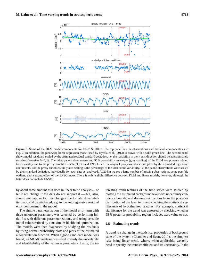
Figure 3. Some of the DLM model components for 10–0◦ S, 20 km. The top panel has the observations and the level components as inFig. 2. In addition, the piecewise linear regression model used byKyrölä et al.(2013) is drawn with a solid green line. The second panelshows model residuals, scaled by the estimated residual standard deviation, i.e. the variability in they axis direction should be approximatelystandard GaussianN(0,1). The other panels show means and 95 % probability envelopes (grey shading) of the DLM components relatedto seasonality and to the proxy variables – solar, QBO and ENSO – i.e. the original proxy variables multiplied by the estimated regressioncoefficients. For the proxy variables, they axis scaling is the percentage of the total ozone variability, i.e. the ozone observations were scaledby their standard deviation, individually for each data set analysed. At 20 km we see a large number of missing observations, some possibleoutliers, and a strong effect of the ENSO index. There is only a slight difference between DLM and linear models, however, although thelatter does not include ENSO.

by about same amount as it does in linear trend analyses – orlet it not change if the data do not support it — but, also,should not capture too fine changes due to natural variabil-ity that could be attributed, e.g. to the autoregressive residualerror component in the model.

The simple parameterization of the model error term withthree unknown parameters was selected by performing ini-tial fits with different parameterizations, and using sensibleinitial values refined by a maximum likelihood optimization.The models were then diagnosed by studying the residualsby using normal probability plots and plots of the estimatedautocorrelation function. When a good candidate model wasfound, an MCMC analysis was used to study the uncertaintyand identifiability of the variance parameters. Lastly, the in-

teresting trend features of the time series were studied byplotting the estimated background level with uncertainty con-fidence bounds, and drawing realizations from the posteriordistribution of the level term and checking the statistical sig-nificance of hypothesized features. For example, statisticalsignificance for the trend was assessed by checking whether95 % posterior probability region included zero value or not.

2.5 Estimating trends

A trend is a change in the statistical properties of backgroundstate of the system (Chandler and Scott, 2011), the simplestcase being linear trend, where, when applicable, we onlyneed to specify the trend coefficient and its uncertainty. In the

www.atmos-chem-phys.net/14/9707/2014/ Atmos. Chem. Phys., 14, 9707–9725, 2014

9714 M. Laine et al.: Time-varying trends in stratospheric ozone

1.4

1.6

1.8

2

2.2

2.4x 10

12 alt: 34 km, lat: 10° S − 0° S

ozone [1/c

m3]

GOMOS

SAGE II

−5

0

5scaled prediction residuals

GOMOS

SAGE II

−5

0

5

seasonal

GOMOS

SAGE II

[%]

−10−5

05 GOMOS

SAGE II

QBOs

[%]

0246

solar

[%]

GOMOS

SAGE II

1985 1990 1995 2000 2005 2010

−2024

ENSO

[%]

GOMOS

SAGE II

Fig. 4. Some of the DLM model components for 10◦ S–0◦ S, 34 km, see Fig. 3 for explanation. We see

noticeable difference between DLM and linear regression fits drawn with a solid green line on the top panel.

25

Figure 4. Some of the DLM model components for 10–0◦ S, 34 km, see Fig.3 for explanation. We see noticeable difference between DLMand linear regression fits drawn with a solid green line on the top panel.

Table 1. Specification of priors for auxiliary model parameters estimated by MCMC. The prior distributions for the model error standarddeviation parameters were log-normal, logN(log(µ),σ2) with values ofµ andσ given in the table. For simplicity, the same relative priorsare used in all the altitude–latitude regions. In Fig.1 the prior distributions are plotted together with MCMC chain histograms that estimatethe posterior distributions for one altitude-latitude region.

Estimated parameter Prior meanµ Prior scaleσ

Trend standard deviation,σtrend 1/12 % of O3 mean 1Seasonal standard deviation,σseas 1 % of O3 variability 2Autoregressive standard deviation,σAR 30 % of O3 variability 2

Autoregressive coefficient,ρ prior is GaussianN(0.45,0.52) truncated to[0,1]

companion paper (Kyrölä et al., 2013) the trend and a changein the trend is studied by using a piecewise linear model witha predefined change point. Natural systems evolve contin-uously in time and it is not always appropriate to approxi-mate the background evolution with a constant, or piecewiselinear, trend. Within the state space dynamic linear modelframework, the trend can be defined as the change in the es-timated background level, i.e. the change inµt defined in

Eq. (3). Posterior sampling from the background level pro-vides an efficient method for studying uncertainties in differ-ent trend estimates.

Temporal changes in the system can be studied by visu-ally inspecting the background level and its estimated uncer-tainty. We can draw samples from the posterior distributionof the levelµt to assess hypotheses about the evolution ofthe process. For example, in Sect.3 we study the change in

Atmos. Chem. Phys., 14, 9707–9725, 2014 www.atmos-chem-phys.net/14/9707/2014/

M. Laine et al.: Time-varying trends in stratospheric ozone 9715

the mean ozone level in 10-year periods. We take into ac-count the uncertainty in the model prediction and in the esti-mated variance parameters by sampling possible backgroundlevelsµt from its posterior uncertainty distribution. We willdo this consecutively and, for each sampled realization, cal-culate the 10-year change in the mean ozone for each timet as trend(t) = µt+60− µt−60 (time units in months). Thissample of trends provides us direct way to analyse trends bycalculating, for example, the mean 10-year trend with 95 %uncertainty limits. The general procedure is the following:

1. Using MCMC with the Kalman filter likelihood, pro-duce a sample from the marginal posterior probabilitydistribution of the auxiliary parameters defining the er-ror covariance matrixW and model matrixG.

2. Draw one realization of the matricesG andW using theposterior distribution provided by MCMC in the previ-ous step.

3. Simulate one realization of the model statex1:N usingthe Kalman simulation smoother assuming fixedG andW from the previous step and calculate trend-relatedstatistics of interest from this realization.

4. Repeat from step 2 to calculate summaries from the pos-terior distribution of the quantity of interest.

3 Results

The model parameters were fitted separately to each data set,i.e. to each height interval and zonal band. We performedthe analyses using vertical average profile data with both theoriginal interpolated 1 km altitude grid and by forming aver-aged ozone densities for three altitude regions: 25–35, 35–45,and 45–55 km. The 10◦ wide zonal bands start from 60◦ Sand go to 60◦ N. By considering each zonal band indepen-dently and summing several altitudes, we have tried to re-duce the model to a minimum one that still shows interestinglong-term changes and is consistent with our assumptions.Initially, a multivariate estimation was considered by fittingseveral altitudes and zonal bands together, but this compli-cated the analyses considerably and did not gain additionalinsight. In principle, we could use the observations in morerefined resolution and model several time series in one es-timation step, and even use the individual satellite retrievalsinstead of spatio-temporal averages.

Figure2 shows an example of our modelling results in thecombined altitude–latitude region, 40–50◦ N, 35–45 km. Theoriginal data are displayed together with DLM estimates andwith the estimated mean level componentµt that is used tomake statistical inference about the trend. The fits are ob-tained by a Kalman smoother (Eqs.A1–A7 in AppendixA)and the 95 % uncertainty regions by combination of a simula-tion smoother (Eqs.A8–A12) and MCMC. A separate panel(on the lower left side) displays the decadal trend obtained

from the level component using MCMC analysis to accountfor the uncertainty in the variance parameters. Looking at theobservations in a 10-year perspective, the trend has been sta-tistically significantly negative up to the year 1997, as thegrey area stays below zero. After 1997, the 10-year trenddoes not statistically differ from zero. After the DLM decom-position, the model residual term is assumed to be uncorre-lated Gaussian noise. The two lower right panels in Fig.2show residual diagnostics. These are used to look for devi-ations from the modelling assumptions. If the scaled residu-als pass the check of being independent and Gaussian withunit variance, then the fit agrees with our assumptions andmodelling results are consistent with the data. In this casethe residuals are almost perfectly uncorrelated Gaussian withunit variance. The normal probability plot compares empiri-cal quantiles (i.e. order statistics) of the residual to those ob-tained from the theoretical Gaussian distribution and in thecase of normally distributed residuals, the points should staymostly on a straight line, as they do here.

The results from MCMC analysis for the same data set asin Fig. 2, are shown in Fig.1. The figure has the prior proba-bility distributions together with marginal posterior distribu-tions as MCMC chain histograms for the estimated auxiliarymodel parameters (referred asθ in AppendixA). We see thatthe parameter posterior distributions are mostly determinedby the data and not by the prior. The standard deviation ofthe trend,σtrend, is estimated to be relatively small, whichsupports the search for smooth background variability. Thisbehaviour is typical for all the fits done. The variability in theseasonal component has more uncertainty, and it also variesmore between the fits for different altitude–latitude regions.The autoregressive parametersσAR andρ have narrow pos-terior distributions relative to the prior, i.e. these values canbe accurately obtained from the data.

Figures3 and4 show the fitted model components for twoindividual altitudes, 20 and 34 km, both at 10–0◦ S. For theseasonal cycle, we plot the sum of the observed seasonalcomponents,ut,1+ut,2 in Eq. (12); for proxies we plotβizt,i ,i.e. the proxy coefficient times the value of the proxy. Thesefits are provided by the Kalman smoother as in the case ofthe mean levelµt . At 20 km, we see a strong effect of ENSO.The total variability explained by ENSO is about 20 % (i.e.its effect is between−10 and 10 %), which is similar to theeffects of the seasonal variation and of the QBO. AlthoughENSO was not used byKyrölä et al.(2013), the fit by linearregression, shown with a solid green line in the upper panel,does agree reasonably well with the DLM level. At 34 km,there is a clear difference between the DLM fit and the piece-wise linear analysis with change point fixed at year 1997.Non-linear changes in the background level are not capturedby the two-piece linear model. Among the proxy variables,the two QBOs, combined in the figure, have the most signif-icant effect, explaining approximately 10 % of the total vari-ability in ozone at that region.

www.atmos-chem-phys.net/14/9707/2014/ Atmos. Chem. Phys., 14, 9707–9725, 2014

9716 M. Laine et al.: Time-varying trends in stratospheric ozone

−55−45−35−25−15−5 5 15 25 35 45 55202224262830323436384042444648505254565860

altitu

de

[km

]

Seasonal

0

20

40

60

80

100

−55−45−35−25−15−5 5 15 25 35 45 55202224262830323436384042444648505254565860

Solar

0

2

4

6

8

10

−55−45−35−25−15−5 5 15 25 35 45 55202224262830323436384042444648505254565860

latitude

altitu

de

[km

]

QBO

0

5

10

15

20

−55−45−35−25−15−5 5 15 25 35 45 55202224262830323436384042444648505254565860

latitude

ENSO

0

5

10

15

20

Fig. 5. The effects of seasonal variation and of the proxy index variables on the variability of ozone. Here

100% means the observed standard deviation of ozone at each latitude altitude bin. The colouring corresponds

to the range of variability during the whole observation period 1984–2011 of each model component given as

percentages with respect to the total variability in ozone. We see, e.g., that the ENSO index significantly affects

the ozone variability only at 20 km near the equator, where the effect is about 20%, also shown in the lowest

panel of Fig. 3. The maximal solar effect is always less than 10%. Note that the colour scales differ.

26

Figure 5. The effects of seasonal variation and of the proxy index variables on the variability of ozone. Here 100 % means the observedstandard deviation of ozone at each latitude altitude bin. The colouring corresponds to the range of variability during the whole observationperiod 1984–2011 of each model component given as percentages with respect to the total variability in ozone. We see, e.g. that the ENSOindex significantly affects the ozone variability only at 20 km near the equator, where the effect is about 20 %, also shown in the lowest panelof Fig. 3. The maximal solar effect is always less than 10 %. Note that the colour scales differ.

Figure5 shows the effects of the fitted variable for the sea-sonal variation and of the proxy index variables on the totalobserved variability of ozone. We calculated, using the datawith 1 km altitude spacing, the range of variability during thewhole observation period 1984–2011 of each model compo-nent given as percentages with respect to the mean ozonevalue. The ENSO index has a significant effect (about 20 %of the variability) only at 20 km near the equator. Near 60 kmand at higher latitudes, almost all of the ozone variability canbe attributed to seasonality. The maximal solar effect is al-ways less than 10 %.

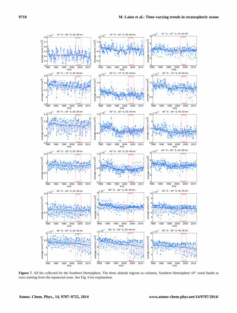
The key results of this paper can be found in Figs.6 and7where we show fits to the ozone time series for 12 latitudebelts and for three altitude regions (25–35 km, 35–45 and45–55 km). We have shown the data points from the mergedSAGE II–GOMOS time series, the DLM fit and the slowlyvarying background levelµt . Overall, it is easy to see thatthe fits usually follow very accurately the data points. Thereare a few scattered outliers, but it is difficult to find any spe-cific pattern for these deviations. As in Fig.2, the solid trendline is the estimated mean levelµt and it is shown with 95 %

uncertainty region. The results for the background curve canbe roughly divided into three classes. The simplest case, acontinuous decay of ozone during the period 1984–2011, isevident in the southernmost latitude band (50–60◦ S) in allaltitude regions. A continuous decay is also present in 50–60◦ N in the lowest altitude region (25–35 km). The secondclass, a recovery between an initial decay and a final decay,is seen from the equator to 50N in the lowest altitude re-gion (25–35 km) and at 40–60◦ N and 35–45 km. The thirdclass covering the rest of the cases shows decay and recov-ery. In the Southern Hemisphere all altitudes and latitudes(10–50◦ S) belong to this class. In the Northern Hemisphereall latitudes in 45–55 km and latitudes from the equator to40◦ N belong to this class.

In Fig. 8 the results of decadal trend analyses are collectedand plotted separately for the three altitude ranges. The cal-culations are explained in Sect.2.5and as final step 7 in Ap-pendix A. The colouring shows the trend, i.e. the averagechange in±5 years around each time axis point. Blue colourmeans a negative and red a positive trend. The change ismost visible at higher altitudes (45–55 and 35–45 km). At the

Atmos. Chem. Phys., 14, 9707–9725, 2014 www.atmos-chem-phys.net/14/9707/2014/

M. Laine et al.: Time-varying trends in stratospheric ozone 9717

1985 1990 1995 2000 2005 20101.5

2

2.5

3x 10

12 50° N − 60° N, 25−35 km

time

avera

ge o

zone [1/c

m3]

GOMOS

SAGE II

1985 1990 1995 2000 2005 20102

3

4

5

6

7

8x 10

11 50° N − 60° N, 35−45 km

time

ave

rag

e o

zo

ne

[1

/cm

3]

GOMOS

SAGE II

1985 1990 1995 2000 2005 20104

5

6

7

8

9

10x 10

10 50° N − 60° N, 45−55 km

time

ave

rag

e o

zo

ne

[1

/cm

3]

GOMOS

SAGE II

1985 1990 1995 2000 2005 20102

2.5

3

3.5x 10

12 40° N − 50° N, 25−35 km

time

ave

rag

e o

zo

ne

[1

/cm

3]

GOMOS

SAGE II

1985 1990 1995 2000 2005 20104

5

6

7

8x 10

11 40° N − 50° N, 35−45 km

time

ave

rag

e o

zo

ne

[1

/cm

3]

GOMOS

SAGE II

1985 1990 1995 2000 2005 20105

6

7

8

9x 10

10 40° N − 50° N, 45−55 km

time

ave

rag

e o

zo

ne

[1

/cm

3]

GOMOS

SAGE II

1985 1990 1995 2000 2005 20102

2.5

3

3.5x 10

12 30° N − 40° N, 25−35 km

time

ave

rag

e o

zo

ne

[1

/cm

3]

GOMOS

SAGE II

1985 1990 1995 2000 2005 20105

5.5

6

6.5

7

7.5

8x 10

11 30° N − 40° N, 35−45 km

time

ave

rag

e o

zo

ne

[1

/cm

3]

GOMOS

SAGE II

1985 1990 1995 2000 2005 20106

6.5

7

7.5

8

8.5

9x 10

10 30° N − 40° N, 45−55 km

timea

ve

rag

e o

zo

ne

[1

/cm

3]

GOMOS

SAGE II

1985 1990 1995 2000 2005 20102.5

3

3.5x 10

12 20° N − 30° N, 25−35 km

time

avera

ge o

zone [1/c

m3]

GOMOS

SAGE II

1985 1990 1995 2000 2005 20105.5

6

6.5

7

7.5x 10

11 20° N − 30° N, 35−45 km

time

avera

ge o

zone [1/c

m3]

GOMOS

SAGE II

1985 1990 1995 2000 2005 20106

6.5

7

7.5

8

8.5

9x 10

10 20° N − 30° N, 45−55 km

time

avera

ge o

zone [1/c

m3]

GOMOS

SAGE II

1985 1990 1995 2000 2005 20102.5

3

3.5

4x 10

12 10° N − 20° N, 25−35 km

time

ave

rag

e o

zo

ne

[1

/cm

3]

GOMOS

SAGE II

1985 1990 1995 2000 2005 20106

6.5

7

7.5x 10

11 10° N − 20° N, 35−45 km

time

ave

rag

e o

zo

ne

[1

/cm

3]

GOMOS

SAGE II

1985 1990 1995 2000 2005 20106

6.5

7

7.5

8

8.5

9x 10

10 10° N − 20° N, 45−55 km

time

ave

rag

e o

zo

ne

[1

/cm

3]

GOMOS

SAGE II

1985 1990 1995 2000 2005 20103

3.2

3.4

3.6

3.8x 10

12 00° S − 10° N, 25−35 km

time

ave

rag

e o

zo

ne

[1

/cm

3]

GOMOS

SAGE II

1985 1990 1995 2000 2005 20105.5

6

6.5

7

7.5x 10

11 00° S − 10° N, 35−45 km

time

ave

rag

e o

zo

ne

[1

/cm

3]

GOMOS

SAGE II

1985 1990 1995 2000 2005 20105

5.5

6

6.5

7

7.5

8x 10

10 00° S − 10° N, 45−55 km

time

ave

rag

e o

zo

ne

[1

/cm

3]

GOMOS

SAGE II

Fig. 6. All fits collected for the northern hemisphere. The three altitude regions as columns, northern hemi-

sphere 10◦ zonal bands as rows starting from the northernmost zone. The smooth solid curve shows the esti-

mated background level with 95% probability envelope. The dots are the observations used in the analysis. The

solid line following the observations is the DLM fit obtained by Kalman filter formulas.

27

Figure 6. All fits collected for the Northern Hemisphere. The three altitude regions as columns, Northern Hemisphere 10◦ zonal bands asrows starting from the northernmost zone. The smooth solid curve shows the estimated background level with 95 % probability envelope. Thedots are the observations used in the analysis. The solid line following the observations is the DLM fit obtained by Kalman filter formulas.

www.atmos-chem-phys.net/14/9707/2014/ Atmos. Chem. Phys., 14, 9707–9725, 2014

9718 M. Laine et al.: Time-varying trends in stratospheric ozone

1985 1990 1995 2000 2005 20103.2

3.3

3.4

3.5

3.6

3.7

3.8x 10

12 10° S − 00° S, 25−35 km

time

avera

ge o

zone [1/c

m3]

GOMOS

SAGE II

1985 1990 1995 2000 2005 20105

5.5

6

6.5

7

7.5

8x 10

11 10° S − 00° S, 35−45 km

time

avera

ge o

zone [1/c

m3]

GOMOS

SAGE II

1985 1990 1995 2000 2005 20105

6

7

8

9x 10

10 10° S − 00° S, 45−55 km

time

ave

rag

e o

zo

ne

[1

/cm

3]

GOMOS

SAGE II

1985 1990 1995 2000 2005 20102.8

3

3.2

3.4

3.6x 10

12 20° S − 10° S, 25−35 km

time

avera

ge o

zone [1/c

m3]

GOMOS

SAGE II

1985 1990 1995 2000 2005 20106

6.5

7

7.5

8x 10

11 20° S − 10° S, 35−45 km

time

avera

ge o

zone [1/c

m3]

GOMOS

SAGE II

1985 1990 1995 2000 2005 20106

6.5

7

7.5

8x 10

10 20° S − 10° S, 45−55 km

time

avera

ge o

zone [1/c

m3]

GOMOS

SAGE II

1985 1990 1995 2000 2005 20102.6

2.8

3

3.2

3.4x 10

12 30° S − 20° S, 25−35 km

time

avera

ge o

zone [1/c

m3]

GOMOS

SAGE II

1985 1990 1995 2000 2005 20106

6.5

7

7.5x 10

11 30° S − 20° S, 35−45 km

time

avera

ge o

zone [1/c

m3]

GOMOS

SAGE II

1985 1990 1995 2000 2005 20106.5

7

7.5

8

8.5x 10

10 30° S − 20° S, 45−55 km

timeavera

ge o

zone [1/c

m3]

GOMOS

SAGE II

1985 1990 1995 2000 2005 20102

2.5

3

3.5x 10

12 40° S − 30° S, 25−35 km

time

avera

ge o

zone [1/c

m3]

GOMOS

SAGE II

1985 1990 1995 2000 2005 20105.5

6

6.5

7

7.5x 10

11 40° S − 30° S, 35−45 km

time

avera

ge o

zone [1/c

m3]

GOMOS

SAGE II

1985 1990 1995 2000 2005 20105

6

7

8

9x 10

10 40° S − 30° S, 45−55 km

time

ave

rag

e o

zo

ne

[1

/cm

3]

GOMOS

SAGE II

1985 1990 1995 2000 2005 20102

2.5

3

3.5x 10

12 50° S − 40° S, 25−35 km

time

avera

ge o

zone [1/c

m3]

GOMOS

SAGE II

1985 1990 1995 2000 2005 20104

5

6

7

8x 10

11 50° S − 40° S, 35−45 km

time

ave

rag

e o

zo

ne

[1

/cm

3]

GOMOS

SAGE II

1985 1990 1995 2000 2005 20104

5

6

7

8

9

10x 10

10 50° S − 40° S, 45−55 km

time

ave

rag

e o

zo

ne

[1

/cm

3]

GOMOS

SAGE II

1985 1990 1995 2000 2005 20101

1.5

2

2.5

3x 10

12 60° S − 50° S, 25−35 km

time

avera

ge o

zone [1/c

m3]

GOMOS

SAGE II

1985 1990 1995 2000 2005 20103

4

5

6

7x 10

11 60° S − 50° S, 35−45 km

time

ave

rag

e o

zo

ne

[1

/cm

3]

GOMOS

SAGE II

1985 1990 1995 2000 2005 20102

4

6

8

10x 10

10 60° S − 50° S, 45−55 km

time

ave

rag

e o

zo

ne

[1

/cm

3]

GOMOS

SAGE II

Fig. 7. All fits collected for the southern hemisphere. The three altitude regions as columns, southern hemi-

sphere 10◦ zonal bands as rows starting from the equatorial zone. See Fig. 6 for explanation.

28

Figure 7. All fits collected for the Southern Hemisphere. The three altitude regions as columns, Southern Hemisphere 10◦ zonal bands asrows starting from the equatorial zone. See Fig.6 for explanation.

Atmos. Chem. Phys., 14, 9707–9725, 2014 www.atmos-chem-phys.net/14/9707/2014/

M. Laine et al.: Time-varying trends in stratospheric ozone 9719

1992 1994 1996 1998 2000 2002 2004 2006

−55−45−35−25−15−5

51525354555

time

latitu

de

Ten year trend, 45−55 km

−0.5

0

0.5

1992 1994 1996 1998 2000 2002 2004 2006

−55−45−35−25−15−5

51525354555

time

latitu

de

Ten year trend, 35−45 km

−0.5

0

0.5

1992 1994 1996 1998 2000 2002 2004 2006

−55−45−35−25−15−5

51525354555

time

latitu

de

Ten year trend, 25−35 km

−0.5

0

0.5

Fig. 8. Ten-year trend in percentage change / year from the DLM fits for each altitude region and zonal band.

One individual trend analysis is shown in the lower left panel of Fig. 2.

29

Figure 8. The 10-year trend in percentage change/ year from the DLM fits for each altitude region and zonal band. One individual trendanalysis is shown in the lower left panel of Fig.2.

−12−8

−8−

6

−6

−6

−4

−4−4−4

−4−4

−4

−2

−2 −2

−2

−2

−2

−2

−2−2

−2

0

00

0

0

0

00

0

0

00

2

22

2

2

2

2

2

2

2

444

4

4

4

44

4

4

66

6

6

666

6

8

8

88

8

8

0

0

2

2

2

1010

−2

−2

24

−2

−4

6

−2

8

6

10

0

4

6

10

8

0

−2

0

10

2

12

6

−4

02

Latitude

Altitude [km

]

Trend change 1997−2011 vs. 1984−1997

−50 −40 −30 −20 −10 0 10 20 30 40 5020

25

30

35

40

45

50

55

60

−10

−5

0

5

10

−50 −40 −30 −20 −10 0 10 20 30 40 5020

25

30

35

40

45

50

55

60

Latitude

Altitu

de

[km

]

Difference between DLM and piecewise linear model

−8

−6

−4

−2

0

2

4

6

8

Fig. 9. To compare DLM results to linear regression analysis in Kyrola et al. (2013) we reproduce its Figure 16

by using the DLM approach. The left panel shows the change in ozone trends in % per decade between the

periods 1997–2011 and 1984–1997. The shaded area indicate regions where the trend difference is non zero

with over 95% posterior probability. The right panel shows the differences (in %/decade) between the numbers

that produce the contour plot on the left panel and the corresponding one in Kyrola et al. (2013) (Fig. 16).

30

Figure 9. To compare DLM results to linear regression analysis inKyrölä et al. (2013) we reproduce its Figure 16 by using the DLMapproach. The left panel shows the change in ozone trends in % per decade between the periods 1997–2011 and 1984–1997. The shadedarea indicate regions where the trend difference is nonzero with over 95 % posterior probability. The right panel shows the differences (in% decade−1) between the numbers that produce the contour plot on the left panel and the corresponding one inKyrölä et al.(2013) (Fig. 16).

lower altitudes (25–35 km) there are some visible changes,but they are mostly masked by a larger variability and thenoise level of the satellite observations at these altitudes. Thenorthernmost (50–60◦ N) and the southernmost (60–50◦ Szones differ significantly from the other zones. Looking atthe individual plots (Figs.6 and7), we see some evidence ofinstrument-related differences and one possible explanationcomes from the different non-uniform sampling character-

istics, both temporal and spatial, of SAGE II and GOMOS(Toohey et al., 2013).

One particular feature of interest in the data is the sug-gested stratospheric ozone recovery due to the prohibitionof CFC compounds by the Montreal treaty in 1987. Sev-eral studies indicate a possible turning point around the year1997 (Newchurch et al., 2003; Jones et al., 2009; Steinbrechtet al., 2009). According to our analyses, significant changesin the average background level of ozone can be seen at

www.atmos-chem-phys.net/14/9707/2014/ Atmos. Chem. Phys., 14, 9707–9725, 2014

9720 M. Laine et al.: Time-varying trends in stratospheric ozone

1985 1990 1995 2000 2005 20103.9

4

4.1

4.2

4.3

4.4

4.5

4.6

4.7x 10

12 lat: 40° S − 30° S, alt: 26 km

timeozone [1/c

m3]

GOMOS

SAGE II

1985 1990 1995 2000 2005 20101.5

1.6

1.7

1.8

1.9

2x 10

11 lat: 30° S − 20° S, alt: 45 km

time

ozone [1/c

m3]

GOMOS

SAGE II

1985 1990 1995 2000 2005 20102.2

2.4

2.6

2.8

3

3.2x 10

12 lat: 10° S − 00° S, alt: 32 km

time

ozone [1/c

m3]

GOMOS

SAGE II

1985 1990 1995 2000 2005 20102

2.2

2.4

2.6

2.8

3

3.2x 10

12 lat: 00° S − 10° N, alt: 32 km

time

ozo

ne

[1

/cm

3]

GOMOS

SAGE II

1985 1990 1995 2000 2005 20101.7

1.8

1.9

2

2.1

2.2

2.3

2.4

2.5x 10

11 lat: 40° N − 50° N, alt: 44 km

time

ozo

ne

[1

/cm

3]

GOMOS

SAGE II

1985 1990 1995 2000 2005 20100.7

0.8

0.9

1

1.1

1.2

1.3x 10

11 lat: 50° N − 60° N, alt: 47 km

time

ozone [1/c

m3]

GOMOS

SAGE II

Fig. 10. Comparing DLM and the linear model. Six examples of DLM vs. piecewise linear model fits using data

with 1 km altitude resolution. The solid black line is the piecewise linear trend from Kyrola et al. (2013). The

smooth solid blue line is the background level component of the DLM model with 95% probability envelope.

At 40◦ N–50◦ N and 44 km the methods agree. In the other panels we see differences of various degrees.

31

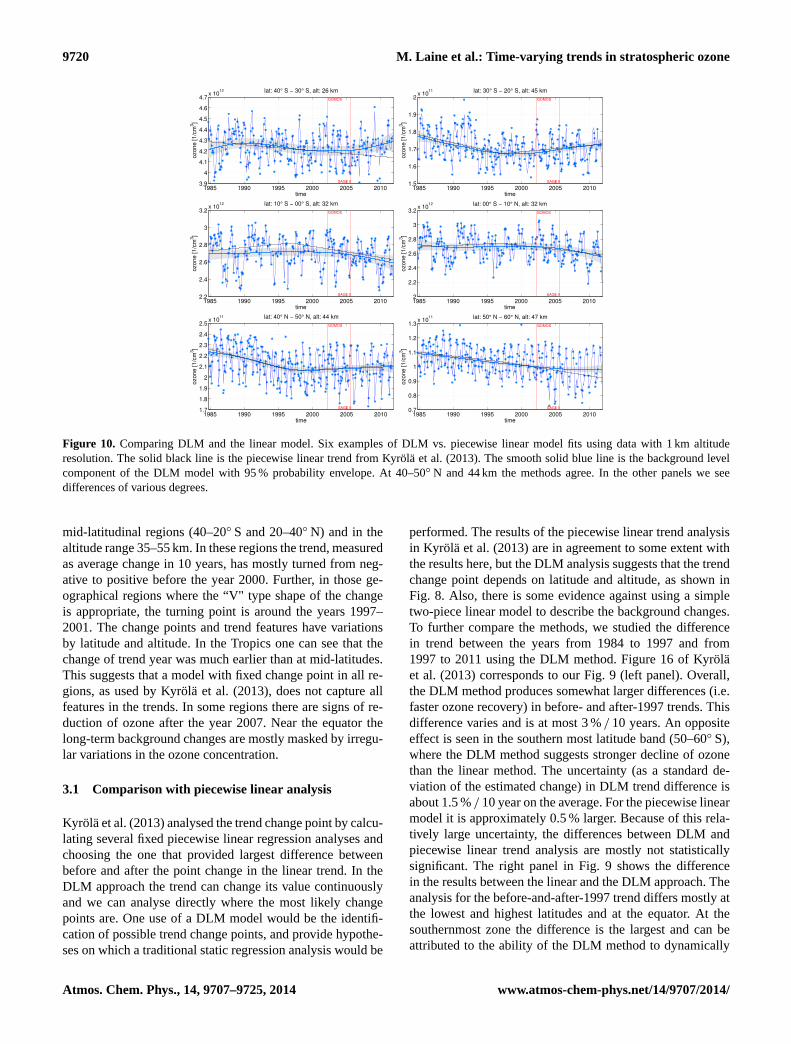
Figure 10. Comparing DLM and the linear model. Six examples of DLM vs. piecewise linear model fits using data with 1 km altituderesolution. The solid black line is the piecewise linear trend fromKyrölä et al.(2013). The smooth solid blue line is the background levelcomponent of the DLM model with 95 % probability envelope. At 40–50◦ N and 44 km the methods agree. In the other panels we seedifferences of various degrees.

mid-latitudinal regions (40–20◦ S and 20–40◦ N) and in thealtitude range 35–55 km. In these regions the trend, measuredas average change in 10 years, has mostly turned from neg-ative to positive before the year 2000. Further, in those ge-ographical regions where the “V" type shape of the changeis appropriate, the turning point is around the years 1997–2001. The change points and trend features have variationsby latitude and altitude. In the Tropics one can see that thechange of trend year was much earlier than at mid-latitudes.This suggests that a model with fixed change point in all re-gions, as used byKyrölä et al.(2013), does not capture allfeatures in the trends. In some regions there are signs of re-duction of ozone after the year 2007. Near the equator thelong-term background changes are mostly masked by irregu-lar variations in the ozone concentration.

3.1 Comparison with piecewise linear analysis

Kyrölä et al.(2013) analysed the trend change point by calcu-lating several fixed piecewise linear regression analyses andchoosing the one that provided largest difference betweenbefore and after the point change in the linear trend. In theDLM approach the trend can change its value continuouslyand we can analyse directly where the most likely changepoints are. One use of a DLM model would be the identifi-cation of possible trend change points, and provide hypothe-ses on which a traditional static regression analysis would be

performed. The results of the piecewise linear trend analysisin Kyrölä et al.(2013) are in agreement to some extent withthe results here, but the DLM analysis suggests that the trendchange point depends on latitude and altitude, as shown inFig. 8. Also, there is some evidence against using a simpletwo-piece linear model to describe the background changes.To further compare the methods, we studied the differencein trend between the years from 1984 to 1997 and from1997 to 2011 using the DLM method. Figure 16 ofKyröläet al. (2013) corresponds to our Fig.9 (left panel). Overall,the DLM method produces somewhat larger differences (i.e.faster ozone recovery) in before- and after-1997 trends. Thisdifference varies and is at most 3 %/ 10 years. An oppositeeffect is seen in the southern most latitude band (50–60◦ S),where the DLM method suggests stronger decline of ozonethan the linear method. The uncertainty (as a standard de-viation of the estimated change) in DLM trend difference isabout 1.5 %/ 10 year on the average. For the piecewise linearmodel it is approximately 0.5 % larger. Because of this rela-tively large uncertainty, the differences between DLM andpiecewise linear trend analysis are mostly not statisticallysignificant. The right panel in Fig.9 shows the differencein the results between the linear and the DLM approach. Theanalysis for the before-and-after-1997 trend differs mostly atthe lowest and highest latitudes and at the equator. At thesouthernmost zone the difference is the largest and can beattributed to the ability of the DLM method to dynamically

Atmos. Chem. Phys., 14, 9707–9725, 2014 www.atmos-chem-phys.net/14/9707/2014/

M. Laine et al.: Time-varying trends in stratospheric ozone 9721

Model componentst time index t = 1, . . . , N

yt observations at time t p vectorxt hidden model states at time t q vectorFt observation operator p × q matrixGt model operator q × q matrixVt observation error covariance matrix p × p matrixWt model error covariance matrix q × q matrixθ static parameter vector k vector

Kalman smoother recursion

p(xt | y1:N, θ ) = N(!x t , !Ct )

Simulation smoother

sample: p(x1:N | y1:N, θ)

MCMC algorithm

sample: p(θ | y1:N)

Monte Carlo sampling

sample: p(x1:N, θ | y1:N)

sample: p(x1:N | y1:N)

Posterior predictive inference of trends

sample: p(trend(x1:N)| y1:N)

Kalman filter likelihood

−2 log p(y1:N |θ) = const +N!

t=1

"(yt − Ft#xt )

T C−1y,t (yt − Ft#xt ) + log(|Cy,t |)

$

State space equations

p(yt |xt , θ) : yt = Ft xt + vt , vt ∼ Np(0, Vt )

p(x t |xt−1, θ) : xt = Gt xt−1 + wt , wt ∼ Nq(0, Wt )

Kalman filter recursion

p(xt |yt, θ) = N(x t , Ct )

p(xt |xt−1, yt−1, θ) = N(!x t , !Ct )

Step 1

Step 4

Step 2

Step 3 Step 5

Step 6

Step 7

Fig. 11. A flowchart showing the dependencies of the DLM calculations explained in Appendix A.

32

Figure 11.A flowchart showing the dependencies of the DLM calculations explained in AppendixA.

adapt to changing seasonal patterns in the observations, seeFig. 7. However, this might be caused by the different spatio-temporal sampling of the two instruments. Further analysisis beyond the scope of this paper – see the discussion in thecompanion paper (Kyrölä et al., 2013).

Figure10 shows six examples of the DLM approach vs.the piecewise linear model fits fromKyrölä et al.(2013). Infive of the cases the conclusions disagree in some respect.In these cases the DLM trend has more variability than thefixed-point model trend – the linear model may miss someimportant features in the data, and the rigidness of the piece-wise linear model may cause spurious results. In some casesthe change point is later than at the beginning of the year1997. However, at those regions where the one-change-pointmodel is valid, the conclusions are the same with both mod-elling approaches.

4 Conclusions

We have shown that a dynamic linear model (DLM) is wellsuited for modelling ozone time series. In contrast to someclassical time series analyses, DLM does not require station-arity, it allows for missing observations and takes uncertain-ties in the observations into account. By using Markov chainMonte Carlo (MCMC) simulation analysis, the uncertaintyin the structural variance parameters can be accounted for.The state space method directly includes a model error term,which makes the analysis more robust to mis-specificationof the model. The analysis allows full statistical uncertaintyquantification, and it is extendible to more refined analyses, ifthose seem necessary. Here, a relatively straightforward andconceptually simple analysis reveals interesting features and,also, validates the more ad hoc choices used in piecewiselinear global analyses, such as in the companion paper byKyrölä et al.(2013).

Trend analysis can be a delicate matter and it is alwayschallenging to give causal explanations. With a properlyset up DLM model we can detect smooth changes in the

www.atmos-chem-phys.net/14/9707/2014/ Atmos. Chem. Phys., 14, 9707–9725, 2014

9722 M. Laine et al.: Time-varying trends in stratospheric ozone

background state. By using proxy variables we can filter outthe effect of known external forcing, such as the solar effect.The DLM analysis provides a method to detect and quantifytrends, but the statistical model itself does not provide expla-nations. It can verify that the observations are consistent withthe selected model. Model diagnostics will eventually falsifywrong models and other badly selected prior specifications.

We used a local linear trend model with two harmonicfunctions for the seasonal effect and four proxy time seriesfor the solar flux, Quasi-Biennial Oscillations and ENSO.An autoregressive model component was used to account forpossible residual autocorrelation. The results show a statis-tically significant change point in the combined SAGE II–GOMOS time series approximately after year 1997 at al-titudes 35–55 km and mid-latitudes, between 50–20◦ S and20–50◦ N. This change point in time varies with latitude andaltitude. There are locations where the estimated changes areopposite to those expected and the length of the data set isstill short relative to some cycles of natural variability inthe atmospheric processes. At the southernmost zones anal-ysed here (60–50◦ S) the DLM method shows larger declineof ozone. This might be attributed to the sampling differ-ences of the two instruments, which is better handled by theDLM method. In many regions the behaviour of the meanozone concentration is too complicated to allow for a sim-ple piecewise linear description. Compared to the two-piecefixed change point linear model used in the companion pa-per, we see stronger recovery of ozone in many regions – thedifference is up to 3 %/ decade.

Atmos. Chem. Phys., 14, 9707–9725, 2014 www.atmos-chem-phys.net/14/9707/2014/

M. Laine et al.: Time-varying trends in stratospheric ozone 9723

Appendix A: Statistical computations for a DLM model

As DLM calculations are based on standard Kalman filter al-gorithms, they can be programmed by most numerical anal-ysis software such as Matlab or the statistical language R.Some additional effort is needed for the parameter estimationby MCMC. We have used Matlab and checked the resultswith the R package DLM (Petris et al., 2009). The Matlabcode we used for the DLM analyses, including the MCMCpart, is available fromhttp://helios.fmi.fi/~lainema/dlm/. Wewill briefly describe the computations here. A flowchart ofthe steps necessary in the computations is given in Fig.11. Aconcise account of the state space approach and Kalman filterbased estimation in time series trend analysis can be found inSect. 5.5 ofChandler and Scott(2011) – for even more de-tails we refer to already cited literature (Harvey, 1990; Petriset al., 2009; Durbin and Koopman, 2012).

We start with the state space equations (1–2), system ma-tricesFt , Gt , Vt , Wt , and the model statext according todefinitions in Sect.2.2. We follow the Bayesian statisticalapproach, where we are interested in the joint posterior un-certainty distribution of the model statesx1:N and the un-known parameters defining the system matrices, given theobservationsy1:N for the whole time series. We collect theextra static parameters (i.e. unknowns in addition to the statex1:N ) into vectorθ and write this probability distribution asp(x1:N ,θ |y1:N ). In the present case, this parameter vector isfour-dimensional:θ = [σtrend,σseas,σAR,ρ]

T .

Step 1

(The steps refer to the flowchart in Fig.11.) If we as-sume that the initial distributions at timet = 0 are avail-able, then the Kalman filter forward recursion (see e.g.Rodgers, 2000) can be used to calculate the distributionof the state vectorxt given the observations up to timet ,p(xt |y1:t ,θ) = N(Sxt ,SCt ), which is Gaussian for eacht =

1,2, . . . ,N . This consists of first calculating, as prior, themean and covariance matrix of one-step-ahead predictedstatesp(xt |xt−1,y1:t−1,θ) = N(xt , Ct ) and the covariancematrix of the predicted observationsCy,t as

xt = GtSxt−1 prior mean forxt , (A1)

Ct = GtSCt−1GT

t + Wt prior covariance forxt , (A2)

Cy,t = Ft CtFTt + Vt covariance for predictingyt (A3)

and then the posterior state and its covariance using theKalman gain matrixK t as

K t = CtFTt C−1

y,t Kalman gain, (A4)

vt = yt − Ft xt prediction residual, (A5)

Sxt = xt + K tvt posterior mean forxt , (A6)

SCt = Ct − K tFt Ct posterior covariance forxt . (A7)

These equations are iterated fort = 1, . . . ,N . As initial val-ues, we can useSx0 = 0 andSC0 = κI , i.e. a vector of zeros

and a diagonal matrix with some large valueκ in the diago-nal. Note that the only matrix inversion required in the aboveformulas is the one related to the observation prediction co-variance matrixCy,t , which is of size 1×1 when we analyseunivariate time series.

Step 2

The Kalman filter provides distributions of the states at eachtime t given the observations up to the current time. Aswe want to do analysis that accounts for all of the ob-servations, we need to have the distributions of the statesfor each time, given all the observationsy1:N . By the lin-earity of the model, these distributions are again Gaussian,p(xt |y1:N ,θ) = N(xt , Ct ). Using the matrices generated bythe Kalman forward recursion, the Kalman smoother back-ward recursion will give us these so-called smoothed statesfor t = N,N −1, . . . ,1 by using the following equations andsettingrN+1 andNN+1 to zero:

L t = Gt − GtK tFt auxiliary variable (A8)

r t = FTt C−1

y,tvt + LTt rt+1 -„- (A9)

Nt = FTt C−1

y,t Ft + LTt Nt+1L t -„- (A10)

xt = xt + Ct rt smoothed state mean (A11)

Ct = Ct − CtNt Ct smoothed state covariance. (A12)

Step 3

In order to study trends, we still need the full joint distri-bution of all the states given all the observations and theparameters, i.e.p(x1:N |y1:N ,θ). This distribution does nothave a closed-form solution. Instead, we can simulate real-izations from it using a so-called simulation smoother al-gorithm (Durbin and Koopman, 2012, Sect. 4.9). The statespace system equations (1) and (2) provide a direct way torecursively produce realizations of both the states and the ob-servations. However, these will be independent of the orig-inal observations.Durbin and Koopman(2012) provide asimple way to produce samples from the distributionx∗

1:N ∼

p(x1:N |y1:N ,θ). Briefly, the simulation smoother algorithmis the following. First, sample from the state space equa-tions to getx1:N andy1:N . Then, use the Kalman smootherwith the new observationsy1:N to get smoothed states˜x1:N .Lastly, add the state residual process to the original smoothedstates to obtainx∗

1:N = x1:N − ˜x1:N + x1:N . This can be re-peated and used to study possible realizations of the modelstates, for example possible mean level dynamics as done inour ozone trend studies.

Step 4

So far, the parameter vectorθ has been assumed fixed.To estimate it, we need the marginal likelihood functionp(y1:N |θ), i.e. the distribution of the observations, given the

www.atmos-chem-phys.net/14/9707/2014/ Atmos. Chem. Phys., 14, 9707–9725, 2014

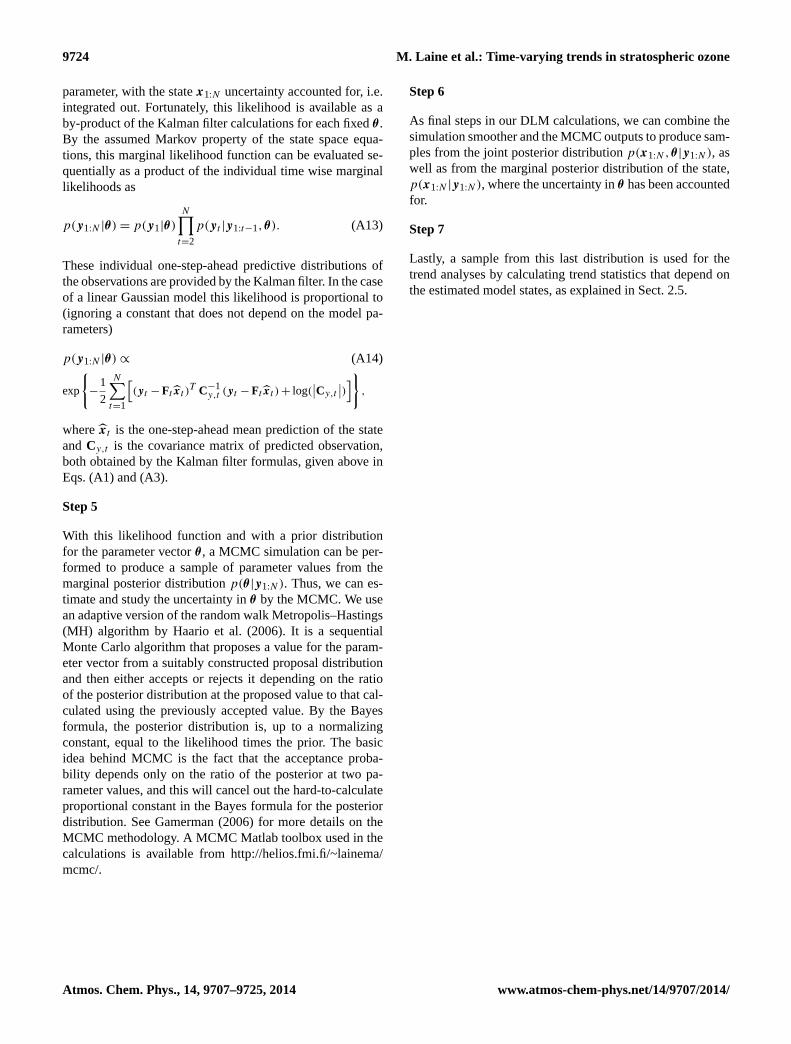
9724 M. Laine et al.: Time-varying trends in stratospheric ozone

parameter, with the statex1:N uncertainty accounted for, i.e.integrated out. Fortunately, this likelihood is available as aby-product of the Kalman filter calculations for each fixedθ .By the assumed Markov property of the state space equa-tions, this marginal likelihood function can be evaluated se-quentially as a product of the individual time wise marginallikelihoods as

p(y1:N |θ) = p(y1|θ)

N∏t=2

p(yt |y1:t−1,θ). (A13)

These individual one-step-ahead predictive distributions ofthe observations are provided by the Kalman filter. In the caseof a linear Gaussian model this likelihood is proportional to(ignoring a constant that does not depend on the model pa-rameters)

p(y1:N |θ) ∝ (A14)

exp

{−

1

2

N∑t=1

[(yt − Ft xt )

T C−1y,t (yt − Ft xt ) + log(

∣∣Cy,t

∣∣)]} ,

wherext is the one-step-ahead mean prediction of the stateandCy,t is the covariance matrix of predicted observation,both obtained by the Kalman filter formulas, given above inEqs. (A1) and (A3).

Step 5

With this likelihood function and with a prior distributionfor the parameter vectorθ , a MCMC simulation can be per-formed to produce a sample of parameter values from themarginal posterior distributionp(θ |y1:N ). Thus, we can es-timate and study the uncertainty inθ by the MCMC. We usean adaptive version of the random walk Metropolis–Hastings(MH) algorithm by Haario et al.(2006). It is a sequentialMonte Carlo algorithm that proposes a value for the param-eter vector from a suitably constructed proposal distributionand then either accepts or rejects it depending on the ratioof the posterior distribution at the proposed value to that cal-culated using the previously accepted value. By the Bayesformula, the posterior distribution is, up to a normalizingconstant, equal to the likelihood times the prior. The basicidea behind MCMC is the fact that the acceptance proba-bility depends only on the ratio of the posterior at two pa-rameter values, and this will cancel out the hard-to-calculateproportional constant in the Bayes formula for the posteriordistribution. SeeGamerman(2006) for more details on theMCMC methodology. A MCMC Matlab toolbox used in thecalculations is available fromhttp://helios.fmi.fi/~lainema/mcmc/.

Step 6

As final steps in our DLM calculations, we can combine thesimulation smoother and the MCMC outputs to produce sam-ples from the joint posterior distributionp(x1:N ,θ |y1:N ), aswell as from the marginal posterior distribution of the state,p(x1:N |y1:N ), where the uncertainty inθ has been accountedfor.

Step 7

Lastly, a sample from this last distribution is used for thetrend analyses by calculating trend statistics that depend onthe estimated model states, as explained in Sect.2.5.

Atmos. Chem. Phys., 14, 9707–9725, 2014 www.atmos-chem-phys.net/14/9707/2014/

M. Laine et al.: Time-varying trends in stratospheric ozone 9725

Acknowledgements.This research has been supported by theAcademy of Finland MIDAT and INQUIRE projects. We thank thevaluable comments given by the editor and the anonymous referees.

Edited by: J. Urban

References

Bates, B. C., Chandler, R. E., and Bowman, A. W.: Trend esti-mation and change point detection in individual climatic seriesusing flexible regression methods, J. Geophys. Res., 117, 1–9,doi:10.1029/2011JD017077, 2012.

Bertaux, J. L., Kyrölä, E., Fussen, D., Hauchecorne, A., Dalaudier,F., Sofieva, V., Tamminen, J., Vanhellemont, F., Fanton D’Andon,O., Barrot, G., Mangin, A., Blanot, L., Lebrun, J. C., Pérot,K., Fehr, T., Saavedra, L., Leppelmeier, G. W., and Fraisse, R.:Global ozone monitoring by occultation of stars: an overview ofGOMOS measurements on ENVISAT, Atmos. Chem. Phys., 10,12091–12148, doi:10.5194/acp-10-12091-2010, 2010.

Chandler, R. E. and Scott, E. M.: Statistical Methods for Trend De-tection and Analysis in the Environmental Sciences, John Wiley& Sons, 388 pp., 2011.

Chu, W. P., McCormick, M. P., Lenoble, J., Brogniez, C., and Pru-vost, P.: SAGE II inversion algorithm, J. Geophys. Res., 94,8339–8351, 1989.

Doucet, A., Freitas, N., and Gordon, N.: Sequential Monte Carlomethods in practice, Statistics for engineering and informationscience, Springer, 581 pp., 2001.

Durbin, T. and Koopman, S.: Time Series Analysis by State SpaceMethods, Oxford Statistical Science Series, Oxford UniversityPress, second edn., 346 pp., 2012.

Gamerman, D.: Markov chain Monte Carlo – Stochastic simulationfor Bayesian inference, Chapman & Hall, second edn., 344 pp.,2006.

Haario, H., Laine, M., Mira, A., and Saksman, E.: DRAM:Efficient adaptive MCMC, Stat. Comp., 16, 339–354,doi:10.1007/s11222-006-9438-0, 2006.

Hamilton, J. D.: Time Series Analysis, Princeton University Press,799 pp., 1994.

Harvey, A. C.: Forecasting, Structural Time Series Models and theKalman Filter, Cambridge University Press, 572 pp., 1990.

Jones, A., Urban, J., Murtagh, D. P., Eriksson, P., Brohede, S., Ha-ley, C., Degenstein, D., Bourassa, A., von Savigny, C., Sonkaew,T., Rozanov, A., Bovensmann, H., and Burrows, J.: Evolutionof stratospheric ozone and water vapour time series studiedwith satellite measurements, Atmos. Chem. Phys., 9, 6055–6075,doi:10.5194/acp-9-6055-2009, 2009.

Kyrölä, E., Laine, M., Sofieva, V., Tukiainen, S., Tamminen, J.,Päivärinta, S., Zawodny, J., and Thomason, L.: Combined SAGEII-GOMOS ozone profile data set for 1984–2011 and trend anal-ysis of the vertical distribution of ozone, Atmos. Chem. Phys.,13, 10645–10658, doi:10.5194/acp-13-10645-2013, 2013.

Lee, J. and Berger, J. O.: Space-time modeling of vertical ozone pro-files, Environmetrics, 14, 617–639, doi:10.1002/env.608, 2003.

Meiring, W.: Oscillations and Time Trends in Stratospheric OzoneLevels: A Functional Data Analysis Approach, J. Am. Stat. As-soc., 102, 788–802, doi:10.1198/016214506000000825, 2007.

Migon, H. S., Gamerman, D., Lopes, H. F., and Ferreira,M. A.: Handbook of Statistics, Vol. 25, Bayesian Think-ing: Mod. Comp., chap. Dynamic Models, 553–588, Elsevier,doi:10.1016/S0169-7161(05)25019-8, 2005.

Newchurch, M. J., Yang, E.-S., Cunnold, D. M., Reinsel, G. C.,Zawodny, J. M., and Russell, J. M.: Evidence for slowdownin stratospheric ozone loss: First stage of ozone recovery, J.Geophys. Res. Atmos., 108, 4507, doi:10.1029/2003JD003471,2003.

Petris, G., Petrone, S., and Campagnoli, P.: Dynamic Linear Modelswith R, Use R!, Springer, 265 pp., 2009.

Rodgers, C. D.: Inverse Methods for Atmospheric Sounding: The-ory and Practice, World Scientific, 238 pp., 2000.

Särkkä, S.: Bayesian Filtering and Smoothing, Institute of Math-ematical Statistics Textbooks, Cambridge University Press, 254pp., 2013.

SPARC: Assessment of Trends in the Vertical Distribution ofOzone, Tech. Rep. 43, World Meteorological OrganizationGlobal Ozone Research and Monitoring Project, WCRP-SPARCReport 1, 1998.

Steinbrecht, W., Claude, H., Schonenborn, F., McDermid, I. S.,Leblanc, T., Godin-Beekmann, S., Keckhut, P., Hauchecorne, A.,van Gijsel, J. A. E., Swart, D. P. J., Bodeker, G. E., Parrish, A.,Boyd, I. S., Kampfer, N., Hocke, K., Stolarski, R. S., Frith, S. M.,Thomason, L. W., Remsberg, E. E., von Savigny, C., Rozanov,A., and Burrows, J. P.: Ozone and temperature trends in the up-per stratosphere at five stations of the Network for the Detectionof Atmospheric Composition Change, Int. J. Remote Sens., 30,3875–3886, doi:10.1080/01431160902821841, 2009.

Toohey, M., Hegglin, M. I., Tegtmeier, S., Anderson, J., Añel,J. A., Bourassa, A., Brohede, S., Degenstein, D., Froidevaux,L., Fuller, R., Funke, B., Gille, J., Jones, A., Kasai, Y., Krüger,K., Kyrölä, E., Neu, J. L., Rozanov, A., Smith, L., Urban, J.,von Clarmann, T., Walker, K. A., and Wang, R. H. J.: Char-acterizing sampling biases in the trace gas climatologies of theSPARC Data Initiative, J. Geophys. Res.-Atmos., 118, 1–16,doi:10.1002/jgrd.50874, 2013.

www.atmos-chem-phys.net/14/9707/2014/ Atmos. Chem. Phys., 14, 9707–9725, 2014