staffing of time-varying queues to achieve time-stable...
TRANSCRIPT
1
Staffing of Time-Varying Queues
To Achieve Time-Stable Performance Project by: Zohar Feldman [email protected] Supervised by: Professor Avishai Mandelbaum [email protected]
Industrial Engineering and Management Technion, Haifa 32000
Israel
June 17th, 2004
Abstract: Following the ideas and infinite-server heuristics of Jennings, Mandelbaum, Massey and Whitt (2001), a simulation-based algorithm is developed for staffing time-varying queues, including abandonment. The algorithm is designed to achieve a given constant probability of delay, say α: α near 0 would lead to a Quality-Driven (QD) operation that emphasized service-quality; α near 1 would lead to an Efficiency-Driven (ED) operation, where the focus is on servers' efficiency; and α strictly between 0 and 1 results in a Quality & Efficiency Driven (QED) operation, with a careful balance between high levels of service-quality and server-efficiency. The algorithm results in a time-varying staffing function of the form ( ) ( ) ( )S t R t R tβ= + : S(t) is the recommended number of servers at time t and R(t) is the given offered load on the system; the constant β reflects service grade that depends on the desired α – the smaller the α (higher service level) the larger the β (more servers) . Under this staffing rule, other performance measures (servers' utilization, average waits, queue-lengths, tail-probabilities) turn out close to being constant as well. Moreover, the functional relation between α and β coincides with those known for stationary models. Thus, we achieve predictably constant (time-stable) performance in a time-varying environment, for operations that are ED, QD or QED. This is clearly desirable but, apriori, not so clearly feasible. Finally, we analyze convergence of our algorithm, which can be provided a theoretical backing within the framework of Markovian Service Networks (Mandelbaum, Massey and Reiman (1998)).

2
1. Introduction 1.1 Background on Services and Call Centers: Service systems (banks, insurance, hospitals, government, etc.) are central in our life, and are vital for our economic viability. Services employ about 60-80% of the workforce in Western Economies, and their importance is sharply on the rise, both within service- and manufacturing-companies. In our service-driven economy, it is estimated that over 70% of the business transactions are carried out over the phone. Most of these transactions are processed by telephone Call Centers, which have become the preferred and prevalent means for companies to communicate with their customers. Indeed, it is estimated that more than 3% of the U.S. workforce is employed in call centers – more that in agriculture! For an overview of the world of call centers and its state-of-art research, readers are referred to the recent review by Gans, Koole and Mandelbaum (2003). The modern call center is a highly complex operation that fuses advanced technology and human beings. But the economic and managerial significance of the latter clearly out-weights the former. More specifically, labor costs (agents' salaries, training, etc.) typically run as high as 70% of the total operating costs of a call center, and attrition rates in call centers reach anywhere from 30% per year (considered low) to over 200% at times. In such circumstances, perhaps the most important operational decision to be made is staffing: what is the appropriate number of telephone agents that are to be accessible for serving calls. Here, over-staffing would have a negative financial effect, while under-staffing would lead to low service-levels and over-worked agents. Figure 1: Hourly call volumes to a medium-size call center
0
500
1000
1500
2000
2500
0 1 2 3 4 5 6 7 8 9 10 11 12 13 14 15 16 17 18 19 20 21 22 23
Hour of Day
Cal
ls p
er H
our
1.2 The Staffing Problem: The staffing problem typically takes the following form: under an existing operational reality, and given a desired service grade (performance measure), one seeks the least number of agents that is required to meet a given service-level constraint. This problem, which has been given a great deal of attention over the years (see Chapter 4 in Gans et. al.), is challenging both

3
theoretically and practically, which is of no surprise. To wit, the natural theoretical settings for the staffing problem are time-varying queues, and these are notoriously difficult to analyze. The practical implication of staffing was already discussed above, and it can be further amplified by considering, for example, a bank employing 10,000 telephone agents and catering to millions of customers per day: clearly, even small gains in operational efficiency or service quality are bound to result in major payoffs. Figure 1 depicts a typical arrival-rate function to a telephone call center. Call volumes are low around midnight, starting to increase in the early hours of the morning, peaking at late morning, then dropping somewhat around 12:00 (lunch break), rising again after noon time, and dropping thereafter to midnight levels. The arrival-rate function is an average of several similar days; the actual number of arrivals, in a given hour on a given day, fluctuates randomly around this average. (As mentioned, the functional shape in Figure 1 is typical; the particular values for the arrival rates were adapted from Green, Kolesar and Soares (2001), in order to benchmark our algorithem; see Section 6.) Staffing planners are thus faced with two sources of variability: predictable variability, namely average time-variations over the day, and random (stochastic) variability around the average. Prevalent staffing algorithms are designed to cope only with stochastic variability, which is enabled by assuming out predictable variability in various ways. Then, however, significant predictable variability would result in excessively fluctuating performance (see Figure 16), which has its clear negative consequences. For example, it would indicate that some parts of the day are over- and others are under-staffed. A reformulation of the staffing problem hence naturally arises, which is the subject of the present study: given a daily performance goal, and faced with predictable and stochastic variability, find the minimal staffing levels that meet this performance goal stably over the day. 1.3 Our Solution to the Staffing Problem In this paper, we present a simulation-based Iterative Staffing Algorithm for time-varying queues. Our algorithm is based on ideas in Whitt (1992) and Jennings, Mandelbaum, Massey and Whitt (1996). (Indeed, the Infinite-Server Approximation in these papers serves as the initial phase of our algorithm, which we then refine iteratively.) Following Jennings et. al. (1996), we assume that, in principle, any number of servers can be assigned at any time; in our implementation, however, time is divided into short intervals (say 5 minutes), and we keep the number of servers fixed over an interval. The service discipline is FCFS, and servers follow an exhaustive service discipline: a server that finishes a shift in the middle of a service will complete the service and sign out only when finished. (Our results prevail also for pre-emptive service disciplines under which servers leave at end-of-shifts and their customers, if any, are moved to the front of the queue.) The contribution of our algorithm is its ability to accommodate very general queueing models, such as Gt/G/st+G queues (queues with abandonment) and more. Specifically, given a target probability of delay, we identify time-varying staffing levels under which the actual probability of delay essentially equals the given target, at all times. Other performance measures, such as the average waiting time, tail delay-probabilities and the probability of abandon, turn out constant over time as well. In fact, global performance measures were found to coincide with the performance measures of a naturally-corresponding stationary system.

4
1.4 An Illustrative Example: Moderate (Im)Patience To facilitate reading, we start with an example that is representative of what is to follow. Consider a queueing system that is faced with an arrival-rate function ( ) ( )100 20 sint tλ = + ⋅ ; service times are exponential having mean 1, and customers' (im)patience is also exponential with mean 1. Our algorithm generates staffing functions, for any given target delay probability α, as in the following three figures. (Blue is the arrival and Red the staffing function.) Figure 2: Quality-Driven (QD) Staffing Function (α=0.1)
05
101520253035404550556065707580859095
100105110115120125130135
0 1 2 3 4 5 6 7 8 9 10 11 12 13 14 15 16 17 18 19 20 21 22 23
Arrived Staffing Offered Load
Figure 3: Efficiency-Driven (ED) Staffing Function (α=0.9)
05
101520253035404550556065707580859095
100105110115120125130
0 1 2 3 4 5 6 7 8 9 10 11 12 13 14 15 16 17 18 19 20 21 22 23
Arrived Staffing Offered Load Figure 4: Quality- and Efficiency-Driven (QED) Staffing Function (α=0.5)
05
101520253035404550556065707580859095
100105110115120125130
0 1 2 3 4 5 6 7 8 9 10 11 12 13 14 15 16 17 18 19 20 21 22 23
Arrived Staffing Offered Load
5
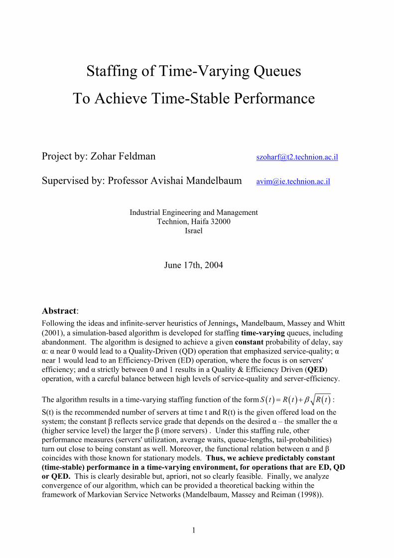
Under the staffing levels arrived at by our algorithm, the target delay probabilities are remarkably accurately (stable) at all times: Figure 5: Delay probability summary for various α's.
Delay Probability
0
0.1
0.2
0.3
0.4
0.5
0.6
0.7
0.8
0.9
1
0 1 2 3 4 5 6 7 8 9 10 11 12 13 14 15 16 17 18 19 20 21 22 23
Target Alpha=0.1 Target Alpha=0.2 Target Alpha=0.3Target Alpha=0.4 Target Alpha=0.5 Target Alpha=0.6Target Alpha=0.7 Target Alpha=0.8 Target Alpha=0.9
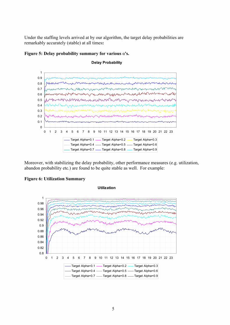
Moreover, with stabilizing the delay probability, other performance measures (e.g. utilization, abandon probability etc.) are found to be quite stable as well. For example: Figure 6: Utilization Summary
Utilization
0.8
0.82
0.84
0.86
0.88
0.9
0.92
0.94
0.96
0.98
1
0 1 2 3 4 5 6 7 8 9 10 11 12 13 14 15 16 17 18 19 20 21 22 23
Target Alpha=0.1 Target Alpha=0.2 Target Alpha=0.3Target Alpha=0.4 Target Alpha=0.5 Target Alpha=0.6Target Alpha=0.7 Target Alpha=0.8 Target Alpha=0.9
6
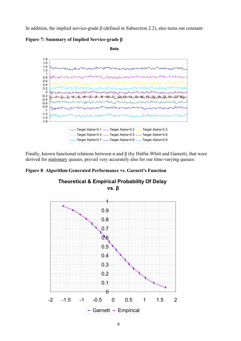
In addition, the implied service-grade β (defined in Subsection 2.2), also turns out constant: Figure 7: Summary of Implied Service-grade β
Beta
-1.6-1.4-1.2
-1-0.8-0.6-0.4-0.2
00.20.40.60.8
11.21.41.61.8
0 1 2 3 4 5 6 7 8 9 10 11 12 13 14 15 16 17 18 19 20 21 22 23
Target Alpha=0.1 Target Alpha=0.2 Target Alpha=0.3Target Alpha=0.4 Target Alpha=0.5 Target Alpha=0.6Target Alpha=0.7 Target Alpha=0.8 Target Alpha=0.9
Finally, known functional relations between α and β (by Halfin-Whitt and Garnett), that were
:varying queues-timeour also for very accuratelyprevail , queuesstationary for derived Figure 8: Algorithm-Generated Performance vs. Garnett's Function
Theoretical & Empirical Probability Of Delay vs. β
0
0.1
0.2
0.3
0.4
0.5
0.6
0.7
0.8
0.9
1
-2 -1.5 -1 -0.5 0 0.5 1 1.5 2
Garnett Empirical
7
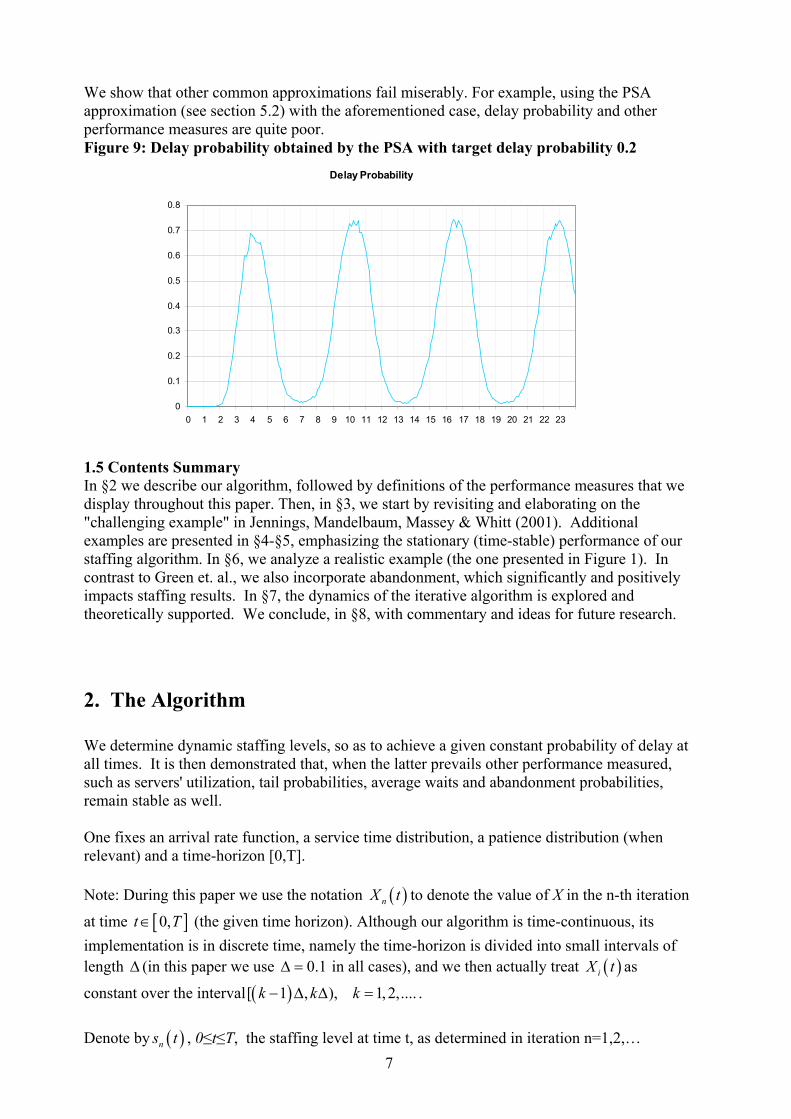
We show that other common approximations fail miserably. For example, using the PSA approximation (see section 5.2) with the aforementioned case, delay probability and other performance measures are quite poor. Figure 9: Delay probability obtained by the PSA with target delay probability 0.2
1.5 Contents Summary In §2 we describe our algorithm, followed by definitions of the performance measures that we display throughout this paper. Then, in §3, we start by revisiting and elaborating on the "challenging example" in Jennings, Mandelbaum, Massey & Whitt (2001). Additional examples are presented in §4-§5, emphasizing the stationary (time-stable) performance of our staffing algorithm. In §6, we analyze a realistic example (the one presented in Figure 1). In contrast to Green et. al., we also incorporate abandonment, which significantly and positively impacts staffing results. In §7, the dynamics of the iterative algorithm is explored and theoretically supported. We conclude, in §8, with commentary and ideas for future research. 2. The Algorithm We determine dynamic staffing levels, so as to achieve a given constant probability of delay at all times. It is then demonstrated that, when the latter prevails other performance measured, such as servers' utilization, tail probabilities, average waits and abandonment probabilities, remain stable as well. One fixes an arrival rate function, a service time distribution, a patience distribution (when relevant) and a time-horizon [0,T]. Note: During this paper we use the notation ( )nX t to denote the value of X in the n-th iteration
at time [ ]0,t T∈ (the given time horizon). Although our algorithm is time-continuous, its implementation is in discrete time, namely the time-horizon is divided into small intervals of length ∆ (in this paper we use 0.1∆ = in all cases), and we then actually treat ( )iX t as
constant over the interval ( )[ 1 , ), 1, 2,....k k k− ∆ ∆ = . Denote by ( )ns t , 0≤t≤T, the staffing level at time t, as determined in iteration n=1,2,…
Delay Probability
0
0.1
0.2
0.3
0.4
0.5
0.6
0.7
0.8
0 1 2 3 4 5 6 7 8 9 10 11 12 13 14 15 16 17 18 19 20 21 22 23
8
Under this staffing function, let ( )nL t stand for the total number in the system at time t. Our algorithm is initialized with a large enough number of servers ( ( )0s ⋅ ≡ ∞ , or ample servers). The probability of delay (i.e. all servers are busy upon arrival) is then negligible. The algorithm performs iteratively the following steps, until convergence is obtained. Here, convergence means that the staffing levels do not change after an iteration. (Practically, they are allowed to change by some threshold)
9
2.1. The Algorithm: - Evaluate the distribution of ( )iL t , for all t ≥0, using simulation;
- Determine ( )1is t+ as follows:
( ) ( ){ }{ }1 arg min : , 0i is t c P L t c t Tα+ = ∈ ≥ < ≤ ≤ ; (1.1)
- Check stopping condition: If ( ) ( )1i is s τ+ ∞
⋅ − ⋅ ≤ , then ( )1is + ⋅ is the proposed staffing level; Otherwise, advance to the next iteration. Denote by ∞ the last iteration of the algorithm (iteration of stopping). Then, the algorithm converges to a staffing function ( )s∞ ⋅ for which ( ) ( ){ }P L t s t α∞ ∞≥ ≈ , 0≤t≤T. Note: In this paper we use τ=1. 2.2. Performance Measures – throughout this paper we present several performance measures. Their definition and method of calculations will now be described. Most measures are time-varying. We define them for each time-interval t, and graph their values as function over [ ]0,t T∈ . Other measures are global. They are calculated either as total counts (e.g. fraction abandoning during [0,T]), or via time-averages. Note: We use T=24 in our simulations. Delay probability in interval t, calculated by the fraction of customers who are not served immediately upon arrival, out of all arriving customers during the t time-interval. Namely, for a single replication, it is given by:
( ){ }
{ }
1 _ _ _ _ _ _
1 _ _ _ _ _ _i
i
customer i enterd queue at interval tt
customer i enterd system at interval tα =
∑∑
(1.2)
We display ( )tα that is averaged over all replications. Average waiting time in interval t, calculated by the average waiting time of all customers arriving during the t time-interval.
( ){ }
{ }
1 _ _ _ _ _ _
1 _ _ _ _ _ _
ii
i
w customer i entered system at interval tW t
customer i entered system at interval t=∑∑
, (1.3)
where iw is the total waiting time of customer i. Again we display ( )W t as averaged over all replications. Average queue length in interval t, taken constant over the time-interval (see page 3). The queue length is averaged over all replications. Tail probability in interval t, calculated as the probability that queue size equals or exceeds 5. Specifically, the indicators ( ) ( ){ }1 5L t s t∞ ∞− ≥ are averaged over all replications.
10
Servers' Utilization in interval t, calculated as the fraction of busy-servers during a time-interval (accounting for servers who are busy only a fraction of the interval):
( )
( )
( )1
s t
ii
bt
s tρ
∞
=
∞
=⋅∆
∑ (1.4)
Where ib denotes the busy time of server i in interval t. The values are again averaged over all replications. Service grade in interval t. In addition to the above measures, we present another parameter called the service gradeβ , which arises from the following "Square-Root Safety Staffing" representation: N R Rβ= + ⋅ (1.5) In this formula, R is the offered load, measured in units of service-time that arrive to the system per unit-of-time. The "square-root" term is safety staffing against stochastic variability. In a time-varying context, the offered load clearly varies with time, and we shall denote it by R(t), 0 t T≤ ≤ . But, less obviously, it is defined in terms of an auxiliary infinite-server system, in which the arrival process and service times coincide with our original system (see Jennings et. al.). More precisely, R(t) it is defined to be the average number of customers (equivalently, average number of busy servers) at time t, for that corresponding infinite-server system. Then, the implied service grade β in all our examples was retrieved by
( ) ( ) ( )( )
s t R tt
R tβ ∞ −
= , 0 t T≤ ≤ , (1.6)
where s∞(t) and R(t) are, respectively, the staffing level arrived at by the algorithm and the offered load, both evaluated at time t (interval t).

11
3. The "Challenging Example" In this section, we explore the "challenging example" presented in Jennings, Mandelbaum, Massey & Whitt (2001). This is an Mt/M/st system, with exponential service times having mean 1, and a non-homogenous Poisson arrival process with the arrival rate function ( ) ( )30 20 sin 5t tλ = + ⋅ ⋅ . As already mentioned, our algorithm is given as input a desired (target) delay probability. In order to examine the performance of the algorithm, we applied it with target delay probabilities α = 0.1, 0.2…, 0.9. For each target α from above, we calculated the corresponding performance measures. We now show summary results graphs for all target delay probabilities Figure 9: Delay probability summary for the Challenging example
Delay Probability
0
0.1
0.2
0.3
0.4
0.5
0.6
0.7
0.8
0.9
1
0 1 2 3 4 5 6 7 8 9 10 11 12 13 14 15 16 17 18 19 20 21 22 23
Target Alpha=0.1 Target Alpha=0.2 Target Alpha=0.3Target Alpha=0.4 Target Alpha=0.5 Target Alpha=0.6Target Alpha=0.7 Target Alpha=0.8 Target Alpha=0.9

12
Figure 10: Implied service gradeβ summary for the Challenging example
Beta
-1.6-1.4-1.2
-1-0.8-0.6-0.4-0.2
00.20.40.60.8
11.21.41.61.8
2
0 1 2 3 4 5 6 7 8 9 10 11 12 13 14 15 16 17 18 19 20 21 22 23
Target Alpha=0.1 Target Alpha=0.2 Target Alpha=0.3Target Alpha=0.4 Target Alpha=0.5 Target Alpha=0.6Target Alpha=0.7 Target Alpha=0.8 Target Alpha=0.9
Figure 11: Utilization summary for the Challenging example
Utilization
0.7
0.75
0.8
0.85
0.9
0.95
1
0 1 2 3 4 5 6 7 8 9 10 11 12 13 14 15 16 17 18 19 20 21 22 23
Target Alpha=0.1 Target Alpha=0.2 Target Alpha=0.3Target Alpha=0.4 Target Alpha=0.5 Target Alpha=0.6Target Alpha=0.7 Target Alpha=0.8 Target Alpha=0.9

13
Figure 12: Tail probability summary for the Challenging example
Tail Probability
0.0
0.1
0.2
0.3
0.4
0.5
0.6
0.7
0.8
0.9
1.0
0 1 2 3 4 5 6 7 8 9 10 11 12 13 14 15 16 17 18 19 20 21 22 23
Target Alpha=0.1 Target Alpha=0.2 Target Alpha=0.3Target Alpha=0.4 Target Alpha=0.5 Target Alpha=0.6Target Alpha=0.7 Target Alpha=0.8 Target Alpha=0.9

14
We chose a set of 3 representing target α 's – 0.1, 0.5, 0.9 to demonstrate further performance behavior. (In some contexts, the set above can be associated with regimes of operation) Figure 13: Target α=0.1: (1) Staffing level, offered load and arrival function, (2) Average queue and waiting time, (3) Waiting time given wait histogram
0
5
10
15
20
25
30
35
40
45
50
55
0 1 2 3 4 5 6 7 8 9 10 11 12 13 14 15 16 17 18 19 20 21 22 23
Arrived Staffing Offered Load
0
0.1
0.2
0.3
0.4
0.5
0.6
0.7
0.8
0 1 2 3 4 5 6 7 8 9 10 11 12 13 14 15 16 17 18 19 20 21 22 230
0.005
0.01
0.015
0.02
0.025
0.03
Average Queue Average Wait
0
0.02
0.04
0.06
0.08
0.1
0.12
00.0
50.1 0.1
50.2 0.2
50.3 0.3
50.4 0.4
50.5 0.5
50.6 0.6
50.7 0.7
50.8 0.8
50.9 0.9
5 1
Wait|Wait>0 Exponential Distribution (mean=0.109)

15
Figure 14: Target α=0.5: (1) Staffing level, offered load and arrival function, (2) average queue and waiting time, (3) Waiting time given wait histogram
0
5
10
15
20
25
30
35
40
45
50
55
0 1 2 3 4 5 6 7 8 9 10 11 12 13 14 15 16 17 18 19 20 21 22 23
Arrived Staffing Offered Load
0
1
2
3
4
5
6
7
8
0 1 2 3 4 5 6 7 8 9 10 11 12 13 14 15 16 17 18 19 20 21 22 230
0.05
0.1
0.15
0.2
0.25
0.3
Average Queue Average Wait
0
0.005
0.01
0.015
0.02
0.025
0.03
0.035
0.04
0.045
00.0
50.10.150.20.2
50.30.350.40.4
5 0.50.55 0.60.6
5 0.70.75 0.80.8
5 0.90.95 1
1.051.11.1
51.21.251.31.3
51.41.451.51.5
51.61.65 1.71.7
5 1.81.85 1.91.9
5 2
Wait|Wait>0 Exponential Distribution (mean=0.301)
16
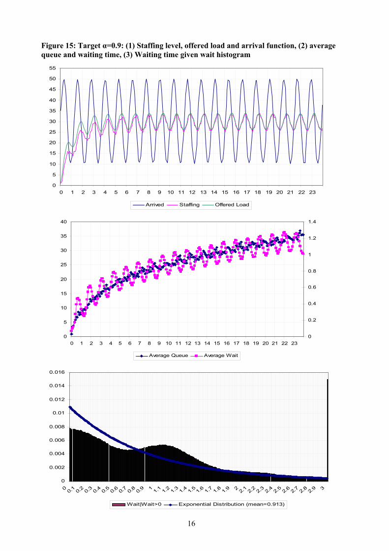
Figure 15: Target α=0.9: (1) Staffing level, offered load and arrival function, (2) average queue and waiting time, (3) Waiting time given wait histogram
0
5
10
15
20
25
30
35
40
45
50
55
0 1 2 3 4 5 6 7 8 9 10 11 12 13 14 15 16 17 18 19 20 21 22 23
Arrived Staffing Offered Load
0
5
10
15
20
25
30
35
40
0 1 2 3 4 5 6 7 8 9 10 11 12 13 14 15 16 17 18 19 20 21 22 230
0.2
0.4
0.6
0.8
1
1.2
1.4
Average Queue Average Wait
0
0.002
0.004
0.006
0.008
0.01
0.012
0.014
0.016
0 0.1 0.2 0.3 0.4 0.5 0.6 0.7 0.8 0.9 1 1.1 1.2 1.3 1.4 1.5 1.6 1.7 1.8 1.9 2 2.1 2.2 2.3 2.4 2.5 2.6 2.7 2.8 2.9 3
Wait|Wait>0 Exponential Distribution (mean=0.913)
17
In (3) of figures 5, 6, 7 we plot the empirical distribution of waiting time given wait (i.e. the waiting time of those who were in fact delayed). Recall that for the stationary M/M/s queue
| 0q qW W > is exponentially distributed. As seen above, the empirical distribution of wait given wait, in our time-varying queue and over all customers, also fits the exponential distribution rather well (the lack of similarity for the case of target α=0.9 occurs mainly due to the fact that measures were taken when system had not reached steady state) . The mean of the exponential distribution was taken to be the overall average waiting time of those who were actually delayed during [0,T].

18
For comparison, we now present performance measures under the SSA approximation. By this we mean a constant staffing level that arises in a naturally corresponding stationary system (i.e. average arrival rate). It suffices to take a representative case in order to notice the very poor and unstable performance. We show the case of target α =0.5. Figure 16: The SSA approx. (target α =0.5 ): (1) Delay probability , (2) average queue and average waiting time, (3) tail probability
0
0.1
0.2
0.3
0.4
0.5
0.6
0.7
0.8
0 1 2 3 4 5 6 7 8 9 10 11 12 13 14 15 16 17 18 19 20 21 22 23
Delay Probability
0
1
2
3
4
5
6
7
8
0 1 2 3 4 5 6 7 8 9 10 11 12 13 14 15 16 17 18 19 20 21 22 230
0.05
0.1
0.15
0.2
0.25
Average Queue Average Wait
0
0.05
0.1
0.15
0.2
0.25
0.3
0.35
0.4
0.45
0.5
0 1 2 3 4 5 6 7 8 9 10 11 12 13 14 15 16 17 18 19 20 21 22 23
Tail Probability

19
When forcing the probability of delay to be constant in time, all other performance measures tend to be stable over all times as well, including the service grade β defined previously. Thus, it seems reasonable to treat α - the probability of delay, and β - the service grade, as constants over all time. One is then lead naturally to a comparison with the Halfin-Whitt function, given by
( )( )
1
{ } 1P delayφ β
α βϕ β
−⎡ ⎤
= = + ⋅⎢ ⎥⎢ ⎥⎣ ⎦
. (2.1)
where ( )ϕ ⋅ and ( )φ ⋅ are the density function and the distribution function of the standard Normal distribution. We plotted the pairs of ( iα , iβ ) along-side the Halfin-Whitt function. We also added ( )φ ⋅ , the
function defined by 1- ( )φ ⋅ , which comes out of the pure infinite-server approximations. Here,
iα was calculated as the fraction of all the delayed customers, out of all arriving customers in [τ ,T] (starting from time τ - the time at which stability was reached); iβ was calculated as the averageβ , over all times starting in [τ ,T]. Figure 17: Comparison of empirical results with the Halfin-Whitt and Normal approx.
Theoretical & Empirical Probability Of Delay vs. β
0
0.1
0.2
0.3
0.4
0.5
0.6
0.7
0.8
0.9
1
-0.5 0 0.5 1 1.5 2
Halfin-Whitt Empirical Normal

20
The excellent match between the empirical and theoretical results implies that our staffing procedure is in fact redundant for the time-varying Erlang-C model! Indeed, one can staff this system, challenging as it may be, simply by calculating the offered load (infinite-server based) at all times, and then using the square-root safety staffing rule (1.5). Here, one chooses ( )1fβ α−= obtained via the Halfin-Whitt function, for any target delay probability α . Remark: The procedure exercised in Jennings et al. uses the Normal curve in the Figure above. Hence, the target delay was not achieved there precisely, and corrections were required. The correction suggested was the use of beta, exactly as above, and the results of our experiments perfectly justify it. The results in Jennings et al are useful in our context as well: they provide simple means for calculating or approximating the offered load. This is in contrast to simulation, which we use in the present study, and which will in fact be necessary in more complicated modes (such as models with abandonment).

21
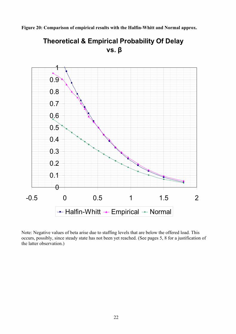
4. QED Example In this section we analyze an example similar to that in the previous section: service times are exponential having mean 1, arrivals are non-homogenous Poisson with the arrival rate function ( ) ( )100 20 sint tλ = + ⋅ . The goal of this example is to examine a larger system (around 100 servers) which, under some parameter values, operates in the QED regime. Figure 18: Delay probability summary for the QED example
Delay Probability
0
0.1
0.2
0.3
0.4
0.5
0.6
0.7
0.8
0.9
1
0 1 2 3 4 5 6 7 8 9 10 11 12 13 14 15 16 17 18 19 20 21 22 23
Target Alpha=0.1 Target Alpha=0.2 Target Alpha=0.3Target Alpha=0.4 Target Alpha=0.5 Target Alpha=0.6Target Alpha=0.7 Target Alpha=0.8 Target Alpha=0.9
Figure 19: Implied service grade β summary for the QED example
Beta
-1.6-1.4-1.2
-1-0.8-0.6-0.4-0.2
00.20.40.60.8
11.21.41.61.8
0 1 2 3 4 5 6 7 8 9 10 11 12 13 14 15 16 17 18 19 20 21 22 23
Target Alpha=0.1 Target Alpha=0.2 Target Alpha=0.3Target Alpha=0.4 Target Alpha=0.5 Target Alpha=0.6Target Alpha=0.7 Target Alpha=0.8 Target Alpha=0.9
22
Figure 20: Comparison of empirical results with the Halfin-Whitt and Normal approx.
Theoretical & Empirical Probability Of Delay vs. β
0
0.1
0.2
0.3
0.4
0.5
0.6
0.7
0.8
0.9
1
-0.5 0 0.5 1 1.5 2
Halfin-Whitt Empirical Normal
Note: Negative values of beta arise due to staffing levels that are below the offered load. This occurs, possibly, since steady state has not been yet reached. (See pages 5, 8 for a justification of the latter observation.)

23
Figure 21: Utilization summary for the QED example
Utilization
0.8
0.82
0.84
0.86
0.88
0.9
0.92
0.94
0.96
0.98
1
0 1 2 3 4 5 6 7 8 9 10 11 12 13 14 15 16 17 18 19 20 21 22 23
Target Alpha=0.1 Target Alpha=0.2 Target Alpha=0.3Target Alpha=0.4 Target Alpha=0.5 Target Alpha=0.6Target Alpha=0.7 Target Alpha=0.8 Target Alpha=0.9
Figure 22: Tail probability summary for the QED example
Tail Probability
0
0.1
0.2
0.3
0.4
0.5
0.6
0.7
0.8
0.9
1
0 1 2 3 4 5 6 7 8 9 10 11 12 13 14 15 16 17 18 19 20 21 22 23
Target Alpha=0.1 Target Alpha=0.2 Target Alpha=0.3Target Alpha=0.4 Target Alpha=0.5 Target Alpha=0.6Target Alpha=0.7 Target Alpha=0.8 Target Alpha=0.9

24
Figure 23: Target α=0.1: (1) Staffing level, offered load and arrival function, (2) average queue and waiting time, (3) Waiting time histogram of those who waited
05
101520253035404550556065707580859095
100105110115120125130135140
0 1 2 3 4 5 6 7 8 9 10 11 12 13 14 15 16 17 18 19 20 21 22 23
Arrived Staffing Offered Load
0
0.1
0.2
0.3
0.4
0.5
0.6
0.7
0.8
0.9
0 1 2 3 4 5 6 7 8 9 10 11 12 13 14 15 16 17 18 19 20 21 22 230
0.001
0.002
0.003
0.004
0.005
0.006
0.007
0.008
0.009
Average Queue Average Wait
0
0.02
0.04
0.06
0.08
0.1
0.12
0.14
0.16
00.0
5 0.1 0.15 0.2 0.2
5 0.3 0.35 0.4 0.4
5 0.5 0.55 0.6 0.6
5 0.7 0.75 0.8 0.8
5 0.9 0.95 1
Wait|Wait>0 Exponential Distribution (mean=0.0658)

25
Figure 24: Target α=0.5: (1) Staffing level, offered load and arrival function, (2) average queue and waiting time, (3) Waiting time histogram of those who waited
05
101520253035404550556065707580859095
100105110115120125130
0 1 2 3 4 5 6 7 8 9 10 11 12 13 14 15 16 17 18 19 20 21 22 23
Arrived Staffing Offered Load
0
2
4
6
8
10
12
0 1 2 3 4 5 6 7 8 9 10 11 12 13 14 15 16 17 18 19 20 21 22 230
0.02
0.04
0.06
0.08
0.1
0.12
0.14
Average Queue Average Wait
0
0.01
0.02
0.03
0.04
0.05
0.06
00.0
5 0.1 0.15 0.2 0.2
5 0.3 0.35 0.4 0.4
5 0.5 0.55 0.6 0.6
5 0.7 0.75 0.8 0.8
5 0.9 0.95 1
Wait|Wait>0 Exponential Distribution (mean=0.18)

26
Figure 25: Target α=0.9: (1) Staffing level, offered load and arrival function, (2) average queue and waiting time, (3) Waiting time histogram of those who waited
05
101520253035404550556065707580859095
100105110115120125130
0 1 2 3 4 5 6 7 8 9 10 11 12 13 14 15 16 17 18 19 20 21 22 23
Arrived Staffing Offered Load
0
10
20
30
40
50
60
70
0 1 2 3 4 5 6 7 8 9 10 11 12 13 14 15 16 17 18 19 20 21 22 230
0.1
0.2
0.3
0.4
0.5
0.6
0.7
0.8
Average Queue Average Wait
0
0.002
0.004
0.006
0.008
0.01
0.012
0.014
0.016
0.018
0 0.1 0.2 0.3 0.4 0.5 0.6 0.7 0.8 0.9 1 1.1 1.2 1.3 1.4 1.5 1.6 1.7 1.8 1.9 2 2.1 2.2 2.3 2.4 2.5 2.6 2.7 2.8 2.9 3
Wait|Wait>0 Exponential Distribution (mean=0.58)
27
5. An Mt/M/st+M Queue 5.1. In this section we add abandonment (due to exponential (im)patience. Thus, we are analyzing the time-varying Palm/Erlang-A queue. The arrival function is ( ) ( )100 20 sint tλ = + ⋅ as before, service times are exponential having mean 1, and, as in the first example, (im)patience is exponential distribution with parameter 1 (mean 1). Figure 26: Delay probability summary for the Erlang-A example
Delay Probability
0
0.1
0.2
0.3
0.4
0.5
0.6
0.7
0.8
0.9
1
0 1 2 3 4 5 6 7 8 9 10 11 12 13 14 15 16 17 18 19 20 21 22 23
Target Alpha=0.1 Target Alpha=0.2 Target Alpha=0.3Target Alpha=0.4 Target Alpha=0.5 Target Alpha=0.6Target Alpha=0.7 Target Alpha=0.8 Target Alpha=0.9
Figure 27: Implied service grade β summary for the Erlang-A example
Beta
-1.6-1.4-1.2
-1-0.8-0.6-0.4-0.2
00.20.40.60.8
11.21.41.61.8
0 1 2 3 4 5 6 7 8 9 10 11 12 13 14 15 16 17 18 19 20 21 22 23
Target Alpha=0.1 Target Alpha=0.2 Target Alpha=0.3Target Alpha=0.4 Target Alpha=0.5 Target Alpha=0.6Target Alpha=0.7 Target Alpha=0.8 Target Alpha=0.9
28
Figure 28: Abandon probability summary for the Erlang-A example
Abandon Probability
0
0.02
0.04
0.06
0.08
0.1
0.12
0.14
0.16
0.18
0 1 2 3 4 5 6 7 8 9 10 11 12 13 14 15 16 17 18 19 20 21 22 23
Taget Alpha=0.1 Taget Alpha=0.2 Taget Alpha=0.3Taget Alpha=0.4 Taget Alpha=0.5 Taget Alpha=0.6Taget Alpha=0.7 Taget Alpha=0.8 Taget Alpha=0.9
Figure 29: Utilization summary for the Erlang-A example
Utilization
0.8
0.82
0.84
0.86
0.88
0.9
0.92
0.94
0.96
0.98
1
0 1 2 3 4 5 6 7 8 9 10 11 12 13 14 15 16 17 18 19 20 21 22 23
Target Alpha=0.1 Target Alpha=0.2 Target Alpha=0.3Target Alpha=0.4 Target Alpha=0.5 Target Alpha=0.6Target Alpha=0.7 Target Alpha=0.8 Target Alpha=0.9

29
Figure 30: Tail probability summary for the Erlang_A example
Tail Probability
0
0.1
0.2
0.3
0.4
0.5
0.6
0.7
0.8
0.9
0 1 2 3 4 5 6 7 8 9 10 11 12 13 14 15 16 17 18 19 20 21 22 23
Target Alpha=0.1 Target Alpha=0.2 Target Alpha=0.3Target Alpha=0.4 Target Alpha=0.5 Target Alpha=0.6Target Alpha=0.7 Target Alpha=0.8 Target Alpha=0.9

30
Figure 31: Target α=0.1: (1) Staffing level, offered load and arrival function, (2) average queue and waiting time, (3) Waiting time histogram of those who waited
05
101520253035404550556065707580859095
100105110115120125130135
0 1 2 3 4 5 6 7 8 9 10 11 12 13 14 15 16 17 18 19 20 21 22 23
Arrived Staffing Offered Load
0
0.1
0.2
0.3
0.4
0.5
0.6
0.7
0.8
0 1 2 3 4 5 6 7 8 9 10 11 12 13 14 15 16 17 18 19 20 21 22 230
0.001
0.002
0.003
0.004
0.005
0.006
0.007
Average Queue Average Wait
0
0.05
0.1
0.15
0.2
0.25
0 0.05 0.1 0.15 0.2 0.25 0.3 0.35 0.4 0.45 0.5
Wait|Wait>0 Exponential Distribution (mean=0.047)

31
Figure 32: Target α=0.5: (1) Staffing level, offered load and arrival function, (2) average queue and waiting time, (3) Waiting time histogram of those who waited
05
101520253035404550556065707580859095
100105110115120125130
0 1 2 3 4 5 6 7 8 9 10 11 12 13 14 15 16 17 18 19 20 21 22 23
Arrived Staffing Offered Load
0
1
2
3
4
5
6
0 1 2 3 4 5 6 7 8 9 10 11 12 13 14 15 16 17 18 19 20 21 22 230
0.005
0.01
0.015
0.02
0.025
0.03
0.035
0.04
0.045
0.05
Average Queue Average Wait
0
0.02
0.04
0.06
0.08
0.1
0.12
0 0.05 0.1 0.15 0.2 0.25 0.3 0.35 0.4 0.45 0.5
Wait|Wait>0 Exponential Distribution (mean=0.084)

32
Figure 33: Target α=0.9: (1) Staffing level, offered load and arrival function, (2) average queue and waiting time, (3) Waiting time histogram of those who waited
05
101520253035404550556065707580859095
100105110115120125130
0 1 2 3 4 5 6 7 8 9 10 11 12 13 14 15 16 17 18 19 20 21 22 23
Arrived Staffing Offered Load
0
2
4
6
8
10
12
14
16
18
0 1 2 3 4 5 6 7 8 9 10 11 12 13 14 15 16 17 18 19 20 21 22 230
0.02
0.04
0.06
0.08
0.1
0.12
0.14
0.16
Average Queue Average Wait
0
0.01
0.02
0.03
0.04
0.05
0.06
0 0.1 0.2 0.3 0.4 0.5 0.6 0.7 0.8 0.9 1
Wait|Wait>0 Exponential Distribution (mean=0.174)

33
Figure 34: Comparison of empirical results with the Garnett approximation
Theoretical & Empirical Probability Of Delay vs. β
0
0.1
0.2
0.3
0.4
0.5
0.6
0.7
0.8
0.9
1
-2 -1.5 -1 -0.5 0 0.5 1 1.5 2
Garnett Empirical
Note: The above graph compares the empirical probability of delay with the corresponding delay-function that arises in Garnett et al (2003). The two functions are indeed remarkably close. In the above, we are using exponential (im)patience with mean 1.
34
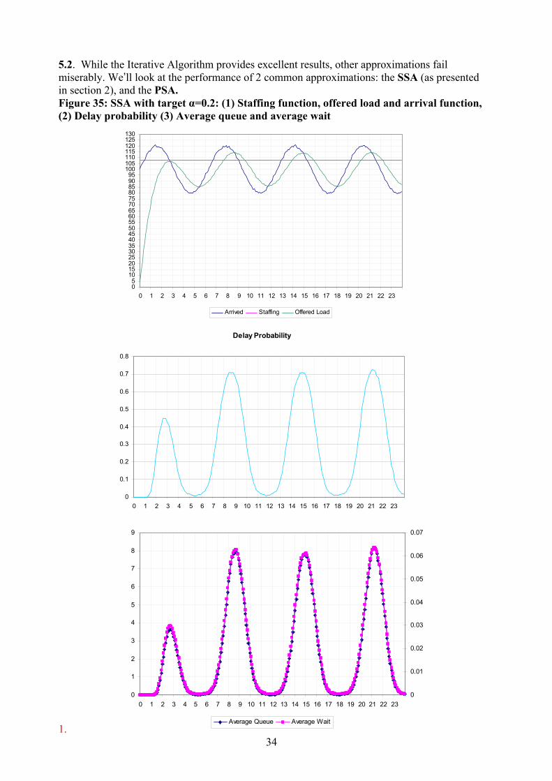
5.2. While the Iterative Algorithm provides excellent results, other approximations fail miserably. We’ll look at the performance of 2 common approximations: the SSA (as presented in section 2), and the PSA. Figure 35: SSA with target α=0.2: (1) Staffing function, offered load and arrival function, (2) Delay probability (3) Average queue and average wait
05
101520253035404550556065707580859095
100105110115120125130
0 1 2 3 4 5 6 7 8 9 10 11 12 13 14 15 16 17 18 19 20 21 22 23
Arrived Staffing Offered Load
1.
0
1
2
3
4
5
6
7
8
9
0 1 2 3 4 5 6 7 8 9 10 11 12 13 14 15 16 17 18 19 20 21 22 230
0.01
0.02
0.03
0.04
0.05
0.06
0.07
Average Queue Average Wait
Delay Probability
0
0.1
0.2
0.3
0.4
0.5
0.6
0.7
0.8
0 1 2 3 4 5 6 7 8 9 10 11 12 13 14 15 16 17 18 19 20 21 22 23

35
The PSA – Point-wise Stationary Approximation. Time-varying staffing levels, based on steady-state M/M/s, with λ= λ(t), at each time t Figure 36: PSA target α=0.2: (1) Staffing function, offered load and arrival function, (2) Delay probability (3) Average queue and average wait
05
101520253035404550556065707580859095
100105110115120125130135140
0 1 2 3 4 5 6 7 8 9 10 11 12 13 14 15 16 17 18 19 20 21 22 23
Arrived Staffing Offered Load
0
1
2
3
4
5
6
7
8
9
0 1 2 3 4 5 6 7 8 9 10 11 12 13 14 15 16 17 18 19 20 21 22 230
0.01
0.02
0.03
0.04
0.05
0.06
0.07
0.08
0.09
Average Queue Average Wait
Delay Probability
0
0.1
0.2
0.3
0.4
0.5
0.6
0.7
0.8
0 1 2 3 4 5 6 7 8 9 10 11 12 13 14 15 16 17 18 19 20 21 22 23

36
5.3. Here, we give an example of a case with very impatient customers. the arrival rate ( ) ( )100 20 sint tλ = + ⋅ , service times are exponential having mean 1, and (im)patience is
exponential with parameter 5 (mean 0.2). Figure 37: Delay probability summary for the impatient Erlang-A example
Delay Probability
0
0.1
0.2
0.3
0.4
0.5
0.6
0.7
0.8
0.9
1
0 1 2 3 4 5 6 7 8 9 10 11 12 13 14 15 16 17 18 19 20 21 22 23
Target Alpha=0.1 Target Alpha=0.2 Target Alpha=0.3Target Alpha=0.4 Target Alpha=0.5 Target Alpha=0.6Target Alpha=0.7 Target Alpha=0.8 Target Alpha=0.9
Figure 38: Implied service grade β summary for the impatient Erlang-A example
Beta
-3.2-3
-2.8-2.6-2.4-2.2
-2-1.8-1.6-1.4-1.2
-1-0.8-0.6-0.4-0.2
00.20.40.60.8
11.21.41.61.8
0 1 2 3 4 5 6 7 8 9 10 11 12 13 14 15 16 17 18 19 20 21 22 23
Target Alpha=0.1 Target Alpha=0.2 Target Alpha=0.3Target Alpha=0.4 Target Alpha=0.5 Target Alpha=0.6Target Alpha=0.7 Target Alpha=0.8 Target Alpha=0.9
37
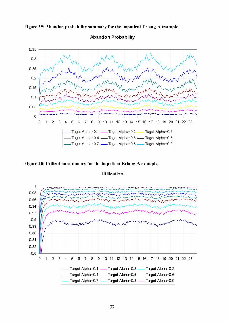
Figure 39: Abandon probability summary for the impatient Erlang-A example
Abandon Probability
0
0.05
0.1
0.15
0.2
0.25
0.3
0.35
0 1 2 3 4 5 6 7 8 9 10 11 12 13 14 15 16 17 18 19 20 21 22 23
Taget Alpha=0.1 Taget Alpha=0.2 Taget Alpha=0.3Taget Alpha=0.4 Taget Alpha=0.5 Taget Alpha=0.6Taget Alpha=0.7 Taget Alpha=0.8 Taget Alpha=0.9
Figure 40: Utilization summary for the impatient Erlang-A example
Utilization
0.8
0.82
0.84
0.86
0.88
0.9
0.92
0.94
0.96
0.98
1
0 1 2 3 4 5 6 7 8 9 10 11 12 13 14 15 16 17 18 19 20 21 22 23
Target Alpha=0.1 Target Alpha=0.2 Target Alpha=0.3Target Alpha=0.4 Target Alpha=0.5 Target Alpha=0.6Target Alpha=0.7 Target Alpha=0.8 Target Alpha=0.9
38
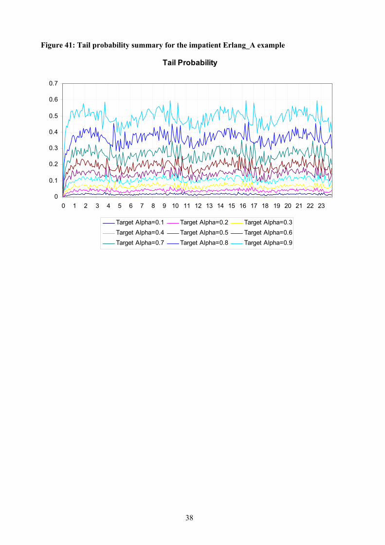
Figure 41: Tail probability summary for the impatient Erlang_A example
Tail Probability
0
0.1
0.2
0.3
0.4
0.5
0.6
0.7
0 1 2 3 4 5 6 7 8 9 10 11 12 13 14 15 16 17 18 19 20 21 22 23
Target Alpha=0.1 Target Alpha=0.2 Target Alpha=0.3Target Alpha=0.4 Target Alpha=0.5 Target Alpha=0.6Target Alpha=0.7 Target Alpha=0.8 Target Alpha=0.9

39
Figure 42: Target α=0.1: (1) Staffing level, offered load and arrival function, (2) average queue and waiting time, (3) Waiting time histogram of those who waited
05
101520253035404550556065707580859095
100105110115120125130135
0 1 2 3 4 5 6 7 8 9 10 11 12 13 14 15 16 17 18 19 20 21 22 23
Arrived Staffing Offered Load
0
0.05
0.1
0.15
0.2
0.25
0.3
0.35
0.4
0.45
0 1 2 3 4 5 6 7 8 9 10 11 12 13 14 15 16 17 18 19 20 21 22 230
0.0005
0.001
0.0015
0.002
0.0025
0.003
0.0035
0.004
Average Queue Average Wait
0
0.05
0.1
0.15
0.2
0.25
0.3
0 0.05 0.1 0.15 0.2 0.25 0.3
Wait|Wait>0 Exponential Distribution (mean=0.031)
40
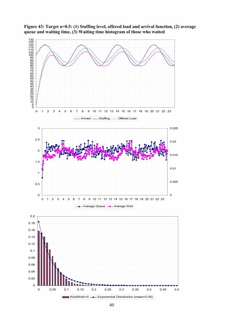
Figure 43: Target α=0.5: (1) Staffing level, offered load and arrival function, (2) average queue and waiting time, (3) Waiting time histogram of those who waited
05
101520253035404550556065707580859095
100105110115120125130
0 1 2 3 4 5 6 7 8 9 10 11 12 13 14 15 16 17 18 19 20 21 22 23
Arrived Staffing Offered Load
0
0.5
1
1.5
2
2.5
3
0 1 2 3 4 5 6 7 8 9 10 11 12 13 14 15 16 17 18 19 20 21 22 230
0.005
0.01
0.015
0.02
0.025
Average Queue Average Wait
0
0.02
0.04
0.06
0.08
0.1
0.12
0.14
0.16
0.18
0.2
0 0.05 0.1 0.15 0.2 0.25 0.3 0.35 0.4 0.45 0.5
Wait|Wait>0 Exponential Distribution (mean=0.05)

41
Figure 44: Target α=0.9: (1) Staffing level, offered load and arrival function, (2) average queue and waiting time, (3) Waiting time histogram of those who waited
05
101520253035404550556065707580859095
100105110115120125130
0 1 2 3 4 5 6 7 8 9 10 11 12 13 14 15 16 17 18 19 20 21 22 23
Arrived Staffing Offered Load
0
1
2
3
4
5
6
7
8
0 1 2 3 4 5 6 7 8 9 10 11 12 13 14 15 16 17 18 19 20 21 22 230
0.01
0.02
0.03
0.04
0.05
0.06
Average Queue Average Wait
0
0.02
0.04
0.06
0.08
0.1
0.12
0 0.1 0.2 0.3 0.4 0.5 0.6 0.7 0.8 0.9 1
Wait|Wait>0 Exponential Distribution (mean=0.096)

42
Figure 45: Comparison of empirical results with the Garnett approximation
Theoretical & Empirical Probability Of Delay vs. β
0
0.1
0.2
0.3
0.4
0.5
0.6
0.7
0.8
0.9
1
-4 -3.5
-3 -2.5
-2 -1.5
-1 -0.5
0 0.5 1 1.5 2
Garnett Empirical
In the above, we are using exponential (im)patience with mean 5.

43
The following graph demonstrate the benefit of staffing a system with consideration to abandonment in contrast to using a simple model with no abandonment. We show the difference between staffing levels for (im)patience distribution with parameters θ=0, 1, 5, 10. Figure 46: Staffing under various (im)patience parameters
Target Alpha=0.5
0
20
40
60
80
100
120
140
0 1 2 3 4 5 6 7 8 9 10 11 12 13 14 15 16 17 18 19 20 21 22 23
Arrived Staffing(θ=0) Staffing(θ=1) Staffing(θ=5) Staffing(θ=10)
Note the area between curves quantifies the savings of labor in time-units. In this case the saving in labor, had one used θ=1, is 113.3 time units, 270 time units for θ=5, and 386 time units when θ=10. The savings of labor increase as α increases.

44
6. Practical Example In this section we consider the practical case introduced in Figure 1. Arrival-rate function is as follows: Figure 47: Arrival function of the practical example
0
500
1000
1500
2000
2500
0 1 2 3 4 5 6 7 8 9 10 11 12 13 14 15 16 17 18 19 20 21 22 23
Hour of Day
Cal
ls p
er H
our
Service Times are exponential having mean 10, and (im)patience is also exponential with parameter 10. Figure 48: Delay probability summary for the practical example
Delay Probability
0
0.1
0.2
0.3
0.4
0.5
0.6
0.7
0.8
0.9
1
0 1 2 3 4 5 6 7 8 9 10 11 12 13 14 15 16 17 18 19 20 21 22 23
Target Alpha=0.1 Target Alpha=0.2 Target Alpha=0.3Target Alpha=0.4 Target Alpha=0.5 Target Alpha=0.6Target Alpha=0.7 Target Alpha=0.8 Target Alpha=0.9

45
Figure 49: Implied service grade β summary for the practical example
Figure 50: Abandon probability summary for the practical example
Abandon Probability
0
0.1
0.2
0.3
0.4
0.5
0.6
0.7
0.8
0 1 2 3 4 5 6 7 8 9 10 11 12 13 14 15 16 17 18 19 20 21 22 23
Taget Alpha=0.1 Taget Alpha=0.2 Taget Alpha=0.3Taget Alpha=0.4 Taget Alpha=0.5 Taget Alpha=0.6Taget Alpha=0.7 Taget Alpha=0.8 Taget Alpha=0.9
Beta
-1.8-1.6-1.4-1.2
-1-0.8-0.6-0.4-0.2
00.20.40.60.8
11.21.41.61.8
0 1 2 3 4 5 6 7 8 9 10 11 12 13 14 15 16 17 18 19 20 21 22 23
Target Alpha=0.1 Target Alpha=0.2 Target Alpha=0.3Target Alpha=0.4 Target Alpha=0.5 Target Alpha=0.6Target Alpha=0.7 Target Alpha=0.8 Target Alpha=0.9

46
Figure 51: Utilization summary for the practical example
Utilization
0.5
0.55
0.6
0.65
0.7
0.75
0.8
0.85
0.9
0.95
1
0 1 2 3 4 5 6 7 8 9 10 11 12 13 14 15 16 17 18 19 20 21 22 23
Target Alpha=0.1 Target Alpha=0.2 Target Alpha=0.3Target Alpha=0.4 Target Alpha=0.5 Target Alpha=0.6Target Alpha=0.7 Target Alpha=0.8 Target Alpha=0.9
47
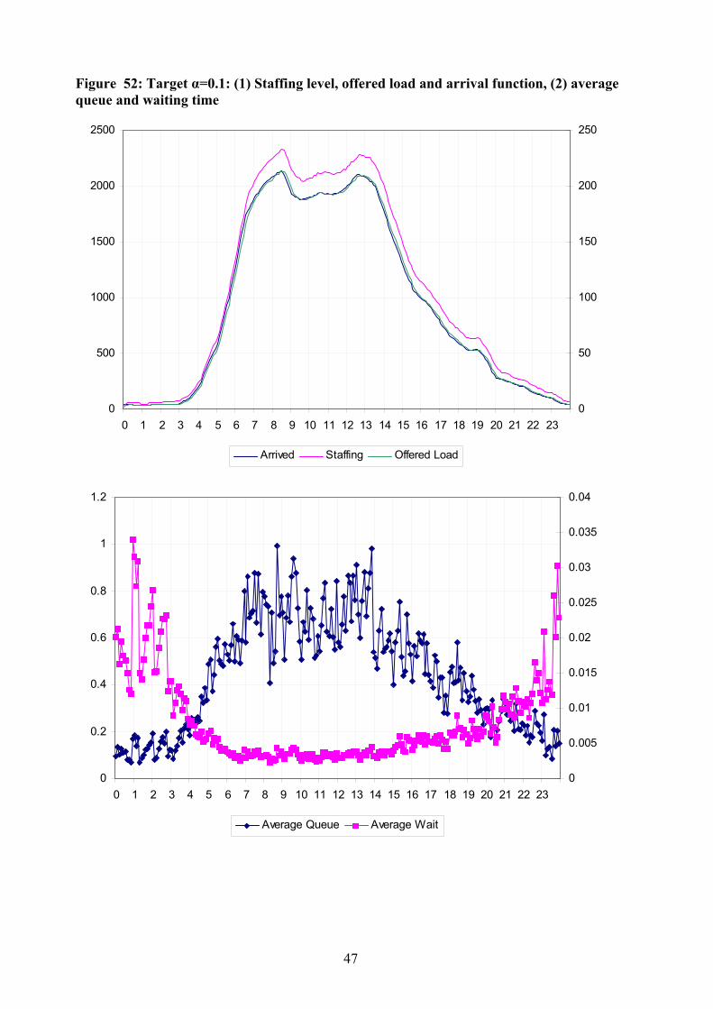
Figure 52: Target α=0.1: (1) Staffing level, offered load and arrival function, (2) average queue and waiting time
0
0.2
0.4
0.6
0.8
1
1.2
0 1 2 3 4 5 6 7 8 9 10 11 12 13 14 15 16 17 18 19 20 21 22 230
0.005
0.01
0.015
0.02
0.025
0.03
0.035
0.04
Average Queue Average Wait
0
500
1000
1500
2000
2500
0 1 2 3 4 5 6 7 8 9 10 11 12 13 14 15 16 17 18 19 20 21 22 230
50
100
150
200
250
Arrived Staffing Offered Load

48
Figure 53: Target α=0.5: (1) Staffing level, offered load and arrival function, (2) average queue and waiting time
0
1
2
3
4
5
6
7
0 1 2 3 4 5 6 7 8 9 10 11 12 13 14 15 16 17 18 19 20 21 22 230
0.02
0.04
0.06
0.08
0.1
0.12
0.14
0.16
0.18
Average Queue Average Wait
0
500
1000
1500
2000
2500
0 1 2 3 4 5 6 7 8 9 10 11 12 13 14 15 16 17 18 19 20 21 22 230
50
100
150
200
250
Arrived Staffing Offered Load

49
Figure 54: Target α=0.9: (1) Staffing level, offered load and arrival function, (2) average queue and waiting time
0
500
1000
1500
2000
2500
0 1 2 3 4 5 6 7 8 9 10 11 12 13 14 15 16 17 18 19 20 21 22 230
50
100
150
200
250
Arrived Staffing Offered Load
0
5
10
15
20
25
0 1 2 3 4 5 6 7 8 9 10 11 12 13 14 15 16 17 18 19 20 21 22 230
0.05
0.1
0.15
0.2
0.25
0.3
0.35
Average Queue Average Wait

50
Figure 55: Comparison of empirical results with the Garnett approximation
Theoretical & Empirical Probability Of Delay vs. β
0
0.1
0.2
0.3
0.4
0.5
0.6
0.7
0.8
0.9
1
-1.5 -1 -0.5 0 0.5 1 1.5
Garnett Empirical
51
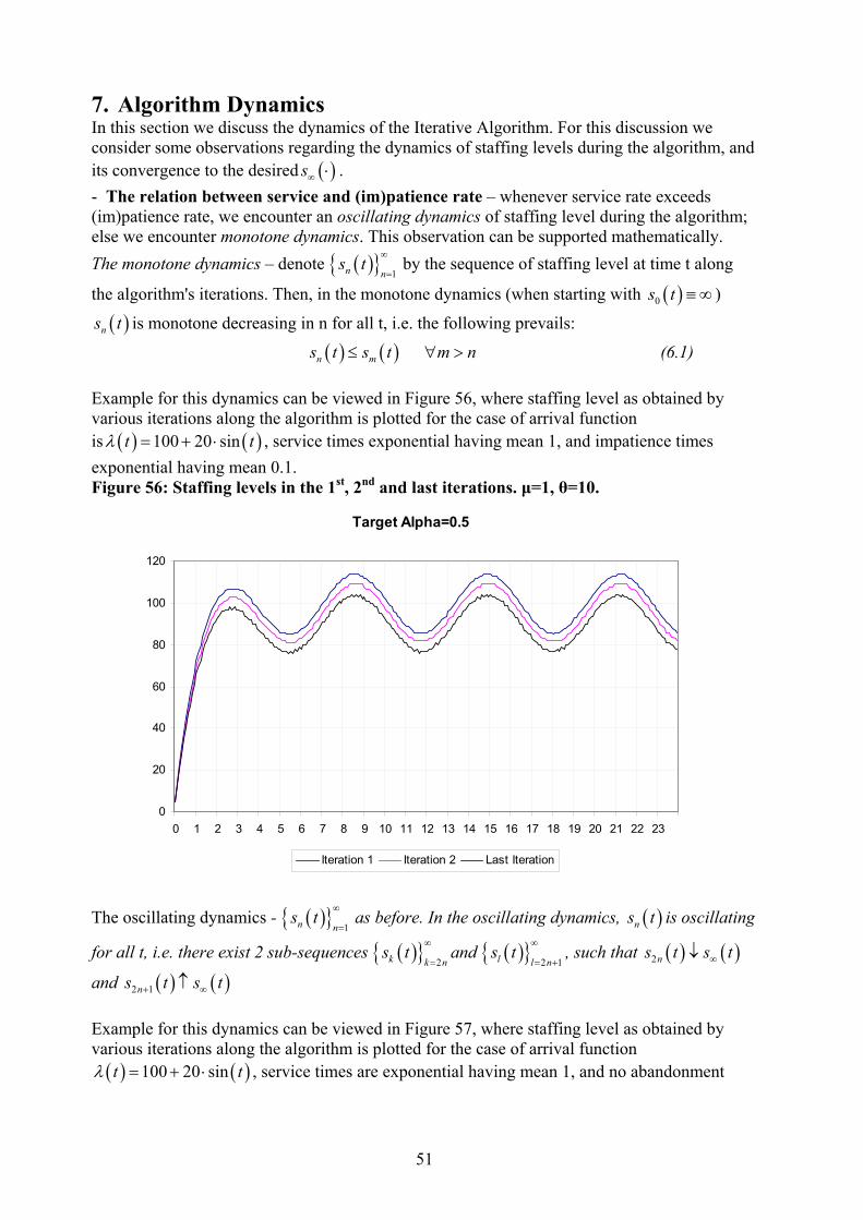
7. Algorithm Dynamics In this section we discuss the dynamics of the Iterative Algorithm. For this discussion we consider some observations regarding the dynamics of staffing levels during the algorithm, and its convergence to the desired ( )s∞ ⋅ . - The relation between service and (im)patience rate – whenever service rate exceeds (im)patience rate, we encounter an oscillating dynamics of staffing level during the algorithm; else we encounter monotone dynamics. This observation can be supported mathematically. The monotone dynamics – denote ( ){ } 1n n
s t∞
= by the sequence of staffing level at time t along
the algorithm's iterations. Then, in the monotone dynamics (when starting with ( )0s t ≡ ∞ )
( )ns t is monotone decreasing in n for all t, i.e. the following prevails:
( ) ( )n ms t s t m n≤ ∀ > (6.1)
Example for this dynamics can be viewed in Figure 56, where staffing level as obtained by various iterations along the algorithm is plotted for the case of arrival function is ( ) ( )100 20 sint tλ = + ⋅ , service times exponential having mean 1, and impatience times exponential having mean 0.1. Figure 56: Staffing levels in the 1st, 2nd and last iterations. µ=1, θ=10.
Target Alpha=0.5
0
20
40
60
80
100
120
0 1 2 3 4 5 6 7 8 9 10 11 12 13 14 15 16 17 18 19 20 21 22 23
Iteration 1 Iteration 2 Last Iteration
The oscillating dynamics - ( ){ } 1n n
s t∞
= as before. In the oscillating dynamics, ( )ns t is oscillating
for all t, i.e. there exist 2 sub-sequences ( ){ } 2k k ns t
∞
=and ( ){ } 2 1l l n
s t∞
= +, such that ( ) ( )2ns t s t∞↓
and ( ) ( )2 1ns t s t+ ∞↑ Example for this dynamics can be viewed in Figure 57, where staffing level as obtained by various iterations along the algorithm is plotted for the case of arrival function ( ) ( )100 20 sint tλ = + ⋅ , service times are exponential having mean 1, and no abandonment

52
Figure 57: Staffing levels in the 1st, 2nd and last iterations'. µ =1, θ=0.
Target Alpha=0.5
0
20
40
60
80
100
120
140
160
0 1 2 3 4 5 6 7 8 9 10 11 12 13 14 15 16 17 18 19 20 21 22 23
Iteration 1 Iteration 2 Final Iteration
- Target delay probability - the oscillating behavior and monotone behavior both tend to the extreme as target delay probability increases, i.e. the range of alternation of staff level increases as target delay probability increases, and thus convergence to ( )s∞ ⋅ requires many more iterations for large delay probabilities. For example, staffing level in the 1st and 2nd iterations, which form the range of the oscillating dynamics, are plotted for both target α=0.1 (figure ) and α=-0.5 (figure ) for the case of arrival function ( ) ( )100 20 sint tλ = + ⋅ , service times are exponential having mean 1, and no abandonment. Figure 58: Range of staffing level for target α=0.1
Target Alpha=0.1
0
20
40
60
80
100
120
140
0 1 2 3 4 5 6 7 8 9 10 11 12 13 14 15 16 17 18 19 20 21 22 23
Iteration 1 Iteration 2

53
Figure 59: Range of staffing level for target α=0.5
Target Alpha=0.5
0
20
40
60
80
100
120
140
160
0 1 2 3 4 5 6 7 8 9 10 11 12 13 14 15 16 17 18 19 20 21 22 23
Iteration 1 Iteration 2
- Time-dependent convergence – Let tI be ( ) ( ){ }inf : ,i jj s t s t i j= ∀ ≥ , then
2 1 2 1t tI I t t≥ ∀ > . An illustration can be viewed in Figure 60. Figure 60: Evolution of convergence during algorithm run-time
Target Alpha=0.5
0
20
40
60
80
100
120
140
160
0 1 2 3 4 5 6 7 8 9 10 11 12 13 14 15 16 17 18 19 20 21 22 23
Iteration 2 Iteration 10 Iteration 30 Last Iteration

54
8. Summary and Future Research An algorithm has been developed that generates staffing functions for which performance is stable in the face of time-varying loads. The results have been found to be remarkably robust, covering the ED, QD and QED operational regimes. Here are some natural "next-steps": - Explore additional queueing systems. We already have partial (successful) results for deterministic service times (for which some theory has been developed and our algorithm can be compared against) and log-normal services (for which no theory is available). More systems to analyze appear in Mandelbaum et. al. (1998), for example queues with abandonment and retrials and priority queues. - Analyze convergence of the algorithm rigorously. The monotone and oscillating convergence, displayed in Section 7, can be explained via stochastic-ordering. For example, oscillating convergence arises when the total-number-in system is stochastically decreasing in the number of servers, and there is monotone convergence if it is stochastically increasing. (Interestingly, the latter does arise naturally: consider, for example, a queue with abandonment in which average (im)patience is shorter than service time; then, more servers would lead to more customers in the system.) - Within the mathematical framework of Service Networks (in Mandelbaum et. el.), we would like to support the algorithm theoretically. Namely, one can hopefully prove that, under proper rescaling, the target probability of delay indeed converges to a time-constant, under some square-root staffing, This has been done already for the moderate-impatience case (equal average patience and service), but further understanding is still required for the general case.
55
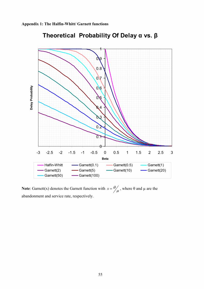
Appendix 1: The Halfin-Whitt/ Garnett functions
Theoretical Probability Of Delay α vs. β
0
0.1
0.2
0.3
0.4
0.5
0.6
0.7
0.8
0.9
1
-3 -2.5 -2 -1.5 -1 -0.5 0 0.5 1 1.5 2 2.5 3Beta
Del
ay P
roba
bilit
y
Halfin-Whitt Garnett(0.1) Garnett(0.5) Garnett(1)Garnett(2) Garnett(5) Garnett(10) Garnett(20)Garnett(50) Garnett(100)
Note: Garnett(x) denotes the Garnett function with x θ
µ= , where θ and µ are the
abandonment and service rate, respectively.

56
References: Gans, N., Koole, G., Mandelbaum, A. Telephone Call Centers: Tutorial, Review and
Research Prospects. Invited review paper by Manufacturing and Service Operations Management (M&SOM), 5 (2), 2003
Garnett O., Mandelbaum A. and Reiman M. Designing a Call Center with Impatient Customers. Manufacturing and Service Operations Management, 4(3), 208-227, 2002
Jennings O., Mandelbaum A., Massey W. and Whitt W. Server Staffing to Meet Time-Varying Demand. Management Science, 42:10 (October 1996), pp. 1383-1394
Mandelbaum A., Massey W.A. and Reiman M. Strong Approximations for Markovian Service Networks. Queueing Systems: Theory and Applications (QUESTA), 30, 149-201, November 1998
Green L., Kolesar P., Soares J. Improving the SIPP Approach For Staffing Service Systems That Have Cyclic Demand. Management Science. July-August 2001