an optimal delay management algorithm from passengers ... · an optimal delay management algorithm...

1

An Optimal Delay Management Algorithm from

Passengers’ Viewpoints considering Whole Railway Network

Satoshi KANAI, Koichi SHIINA, Shingo HARADA, Norio TOMII Chiba Institute of Technology, Department of Computer Science,

2-17-1 Narashino Tsudanuma Chiba 275-0016 Japan, e-mail: [email protected]

Abstract

We propose an algorithm for an optimal delay management. We set passengers’

dissatisfaction of all passengers in the whole railway network as a criterion and developed

an algorithm which seeks for a delay management plan which makes passengers’

dissatisfaction minimum. The algorithm is a combination of simulation and optimization.

Simulation part consists of a train traffic simulator and a passenger flow simulator which

work in parallel. The train traffic simulator forecasts future train diagram considering the

dynamic interaction between trains and passengers. The passenger flow simulator traces

behaviour of all the passengers one by one and calculates how many passengers get on/off

at each station. This information is given to the train traffic simulator and necessary dwell

times are calculated. Passengers’ dissatisfaction is also estimated from the results of the

passenger flow simulation. In the optimization part, we use the tabu search algorithm. We

will show the details of our algorithm together with numerical results using real world

data.

Keywords

Delay Management, Connection, Simulation, Optimization, Meta-heuristics

1 Introduction

In many lines of Japan, timetables in which connections between trains are well

considered are provided. But in case a delay occurs, dispatchers have to make a decision

whether to maintain the connection by making the connecting train wait or to break it so

that the connecting train can depart on time. This decision is called “delay management,”

and is quite an important task from the viewpoints of passengers’ satisfaction. If the

connection is maintained, passengers who transfer do not have to wait, which is very

convenient for them but those who on the connecting train have to wait for some time. In

addition, the train is inevitably delayed and it is quite probable that another delay

management problem would occur subsequently. On the other hand, if the connection is

broken, transferring passengers complain a lot unless there is another train they can catch

without waiting for a long time.

To keep a connection at one occasion may give an influence to the whole railway

network. It is required to make a decision about which connection should be maintained

and which connection should be broken considering the whole timetable and the railway

network. In this paper, we call a plan which consists of series of decisions about

connection for the whole railway network a delay management plan.

Our ambition is to develop an algorithm which gives an optimal delay management

plan in real time when an initial delay is given.

In order to make an optimal delay management plan from a viewpoint of the whole

2

railway network, it is necessary to forecast as exactly as possible how the train schedule

would be considering the influence of the initial delay and the operational constraints of

railways. In addition, in urban areas, it is indispensable to consider the dynamic

interaction between trains and passengers. A dynamic interaction means a phenomenon

such that if a train is delayed for some time, more passengers than usual get on at the next

station and the dwell time becomes longer than usual and the train is delayed more. This

phenomenon is repeated at the subsequent stations and the delay becomes larger and

larger like a snowball. This is because the time necessary for passengers’ getting on and

off becomes longer than the dwell time specified in the timetable. If we ignore the

dynamic interaction, we can get a very poor result of forecast which is useless.

Consideration for the dynamic interaction is especially important when we consider

connections from trains of a main line to trains of feeder lines.

From these discussions, we can conclude that in order to make an optimal delay

management plan:

- We have to focus on passengers (dis)satisfaction not only on delays.

- We have to bring the whole railway network into our eyes because a change at one

scene is quite probable to cause another problem in other places.

- We have to set up a criterion for an optimal delay management from passengers’

viewpoints considering the whole railway network.

- We have to trace behaviour of each passenger including detour or change of his/her

original travel plan. Passengers may change their original travel plan if the timetable

is changed and in order to calculate how much discomfort passengers will suffer, we

need to trace each passenger’s behaviour in detail.

In this paper, we introduce an algorithm for optimal delay management. Our algorithm

consists of a simulation part and an optimization part: the simulation part is actually a

combination of a train traffic simulator and a passenger flow simulator. The train traffic

simulator forecasts the future timetable. The simulator is designed based on PERT

(Program Evaluation and Review Technique). All the operational constraints are

expressed by directed arcs, it can always produce a result in which capacity constraints are

considered and conflicts are resolved. The passenger flow simulator calculates

passenger’s dissatisfaction by simulating behaviour of passengers one by one. These two

simulators work in parallel to simulate the dynamic interaction between trains and

passengers. In the optimization part, we use the taboo search algorithm. The aim of this

algorithm is to seek for a delay management plan which makes the passengers’

dissatisfaction minimum.

This paper is comprised as follows. In Section 2, we describe the delay management

problem together with related works. In Section 3, we introduce our algorithm in detail. In

Section 4, we present numerical results of our algorithm using real world data.

2 Delay Management Problem

2.1 Connection of Trains

There are several types of connection between trains. One is a connection between trains

which run along the same railway line. The second type is a connection between trains

which run along different lines. The third type is a connection between a main line and a

feeder line.

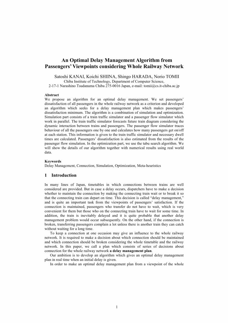
As an example of the connection of the first type, we can point out a connection

between an express train and a local train (see Figure 1). In order to offer an express

3

service, express trains which stop only at major stations are operated. Connection between

an express train and a local train is planned so that the passengers at stations where

express trains do not stop can also get an express service. Usually, connection of this type

should be “mutual.” That is, passengers can transfer both way; from Express to Local and

from Local to Express. But rather exceptionally, there might exist a one way connection;

from Express to Local or from Local to Express. From passengers’ viewpoints, mutual

connection is more desirable.

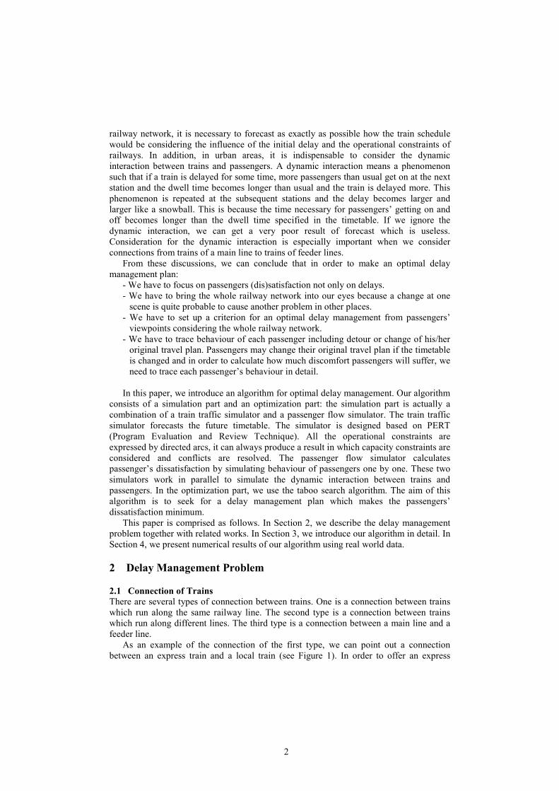
One example of the second type connection is a connection in a quadruple track line.

A good example is a connection between an express train which run along the outer track

and a local train which run along the inner track (Figure 2). Again, connection of this type

should be mutual from passengers’ point of view, but there could be a one way connection

too. Train operation in a quadruple track line is more flexible than a double track line. In a

double track line, breaking a connection of Figure 1 means to change the departing order

of trains. So, drivers must receive an order from dispatchers. On the other hand, in

quadruple track lines, trains on both track run independently and without receiving such

orders from dispatchers, a driver and a conductor can make a decision to break or to

maintain a connection.

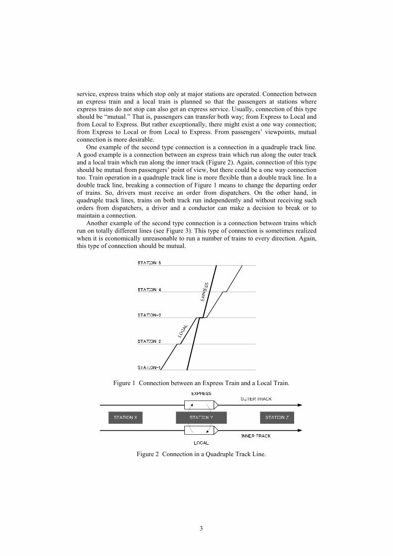
Another example of the second type connection is a connection between trains which

run on totally different lines (see Figure 3). This type of connection is sometimes realized

when it is economically unreasonable to run a number of trains to every direction. Again,

this type of connection should be mutual.

Figure 1 Connection between an Express Train and a Local Train.

Figure 2 Connection in a Quadruple Track Line.

4

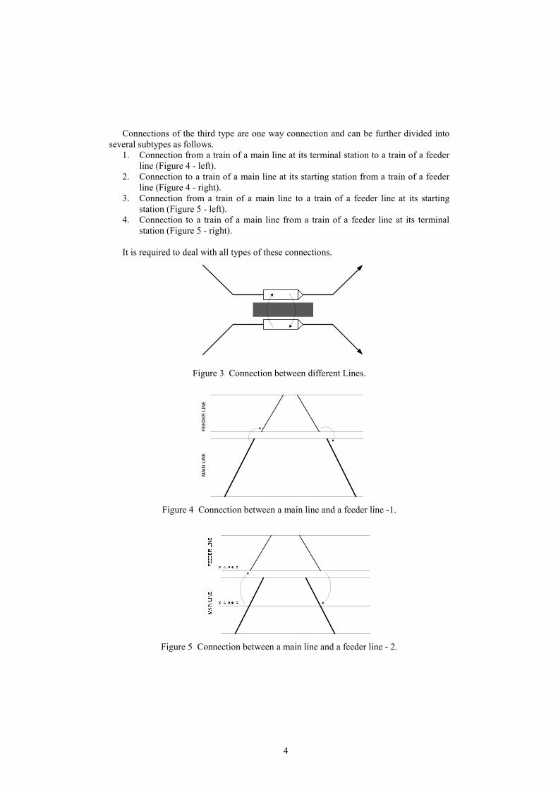
Connections of the third type are one way connection and can be further divided into

several subtypes as follows.

1. Connection from a train of a main line at its terminal station to a train of a feeder

line (Figure 4 - left).

2. Connection to a train of a main line at its starting station from a train of a feeder

line (Figure 4 - right).

3. Connection from a train of a main line to a train of a feeder line at its starting

station (Figure 5 - left).

4. Connection to a train of a main line from a train of a feeder line at its terminal

station (Figure 5 - right).

It is required to deal with all types of these connections.

Figure 3 Connection between different Lines.

Figure 4 Connection between a main line and a feeder line -1.

Figure 5 Connection between a main line and a feeder line - 2.

5

2.2 Delay Management for a Railway Network

At the moment, there are two major problems in delay management. The first one is that

delay management is done “locally.” The other one is that passengers’ dissatisfaction is

not well considered.

Dispatchers usually make a decision whether to maintain or to cancel a connection.

When dispatchers are once informed of a delay of a train, they consult with the current

timetable and decide whether the connection should be maintained or not, considering the

delay of the train and imagining how many passengers are transferring. The decision,

however, is made only considering the initial delay. Influence of the result of delay

management is not explicitly considered. For example, if a train is kept waiting because of

connection, the train is inevitably delayed and if the train has a connection in another

station, there occurs another delay management problem. It might be the case that if we

consider the second delay management problem, we should not have kept the train waiting.

Such a problem might happen all over the railway network. But at present, dispatchers do

not make a decision taking the whole railway network into account, because this problem

is too complicated and too large-sized.

The other problem of the current delay management by dispatchers is that they do not

explicitly think about passengers’ dissatisfaction. They imagine how many passengers are

on board or waiting at stations from their experience, but no one knows if they are correct

or not. Not only the number of passengers but they do not know how far the passengers

travel either, for example, long distance or short distance. Dispatchers, however, should

not be blamed. This problem occurs because there are no equipments from which they can

get information about the situation of passengers on board and at stations.

2.3 Requirements for Delay Management Algorithm

From above discussions, we have set up the following as requirements for a delay

management algorithm.

1. It is required to produce an optimal delay management plan for the whole railway

network.

2. Criteria of optimality must be one from viewpoint of passengers’ satisfaction.

3. It can deal with various kinds of criteria.

There exist various kinds of criteria. Someone may think discomfort by congestion

should be considered as well as the travelling time. Another people may insist

travelling distance should be considered. For example, there might be a difference of

an impression for the same delay time between passengers who travel for a long

distance and those who travel for a short distance. What criterion is used is decided

from managerial or commercial point of view considering the situation of the railway

line, such as frequency of trains, passenger OD and so on. Thus, it is required that the

algorithm is designed so flexible to be able to adopt various kinds of criteria.

4. Dynamic interaction between trains and passengers is implemented as stated earlier.

5. It must trace each passenger’s behaviour in order to estimate passengers’

dissatisfaction assuming passengers take reasonable behaviours.

It is reasonable to assume that passengers want to arrive at their destination as fast as

possible. But they care about congestion and convenience of transfer (it is usually the

case that passengers cannot get a seat in railway lines in urban areas of Japan.

Moreover, some trains are uncomfortably congested). When passengers arrive at a

station, they decide which train to take and where to transfer. But if there is some

change in environment, they might change their route during their trip. For example, if

they get an announcement about a disruption of train traffic, they may change their

6

route or train selections. If the train has become much more congested than they first

expected, they may change trains.

2.4 Related Works

A number of researches have been reported about delay management (see [9]). Gatto

proved that the delay management problem is NP-hard [4]. Schachtebeck proposed an

approach to combine heuristics and integer programming aiming at minimizing the sum of

all delays passengers have plus the sum of all missed connections [8]. Capacity constraints

are also considered in [8]. Dollevoet also uses an integer programming approach and

introduced consideration about re-routing of passengers [3].

But, [7] sets a rather strong assumption that all lines have common period and that all

trains are on time in the next period, which does not hold especially in lines where trains

are running densely. It is reported in [3] that it was impossible to solve a large sized

problem which is still a drawback of integer programming approach even now.

3 An Optimal Delay Management Algorithm for a Railway Network

3.1 Basic Idea - Approach

We take an approach to combine simulation and optimization. In optimization part, we

use meta-heuristics. This is because this approach has merits such as it can simulate

realistic passengers’ behaviour and estimate their dissatisfaction and it can deal with

various kinds of complicated objective functions.

The simulation part of our algorithm simulates train traffic and passenger behaviour.

Passengers’ dissatisfaction is estimated from the results of the simulation part and used as

the criterion for evaluation. The optimization part searches for an optimal delay

management plan which makes passengers’ dissatisfaction minimum for the whole

railway network based on the results of the simulation part.

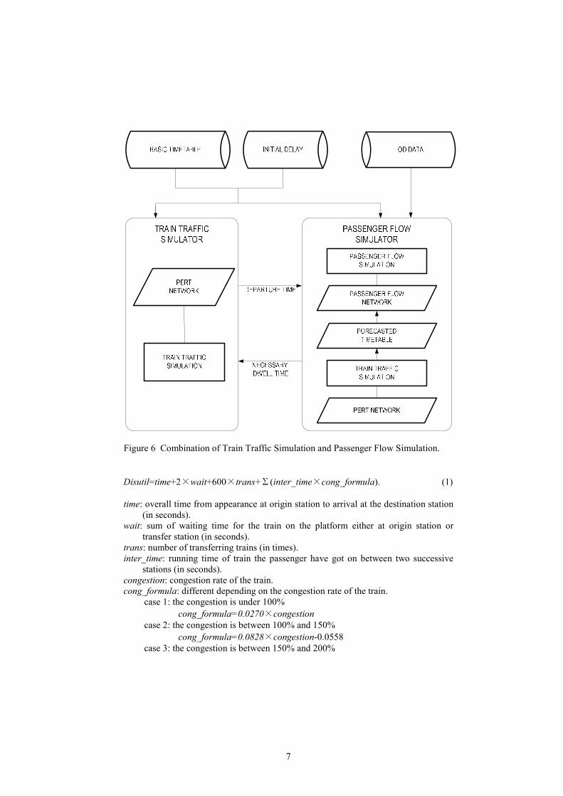
The simulation part consists of two simulators; one is a train traffic simulator and the

other is a passenger flow simulator (see Figure 6). These two simulators work in parallel.

The train traffic simulator simulates future train traffic based on the basic timetable and

the initial delay. The passenger flow simulator traces behaviour of each passenger one by

one. The numbers of passengers who get on/off at each station from each train are

calculated by the passenger flow simulator and the train traffic simulator calculates the

necessary dwell time of the train. Thus, the dynamic interaction between trains and

passengers are simulated. The passenger flow simulator also calculates dissatisfaction of

passengers from their travelling times, waiting times, discomfort from transfer and

congestion inside trains.

3.2 Objective Function for Delay Management from Passengers’ Point of View

We insist that it is important to use criteria with regard to passengers’ dissatisfaction. In

order to express passengers’ dissatisfaction, we use “passengers’ disutility [6].”

Passengers’ disutility function is composed of time needed to arrive at the destination,

experienced waiting time for trains, dwell time in the train cars, exchanging times, and

experienced train congestion, described in Formula (1). The more disutility a passenger

experiences, the more inconvenient he or she feels.

7

Figure 6 Combination of Train Traffic Simulation and Passenger Flow Simulation.

Disutil=time+2×wait+600×trans+∑(inter_time×cong_formula). (1)

time: overall time from appearance at origin station to arrival at the destination station

(in seconds).

wait: sum of waiting time for the train on the platform either at origin station or

transfer station (in seconds).

trans: number of transferring trains (in times).

inter_time: running time of train the passenger have got on between two successive

stations (in seconds).

congestion: congestion rate of the train.

cong_formula: different depending on the congestion rate of the train.

case 1: the congestion is under 100%

cong_formula=0.0270×congestion

case 2: the congestion is between 100% and 150%

cong_formula=0.0828×congestion-0.0558


8




case 5: the congestion is more than 250%


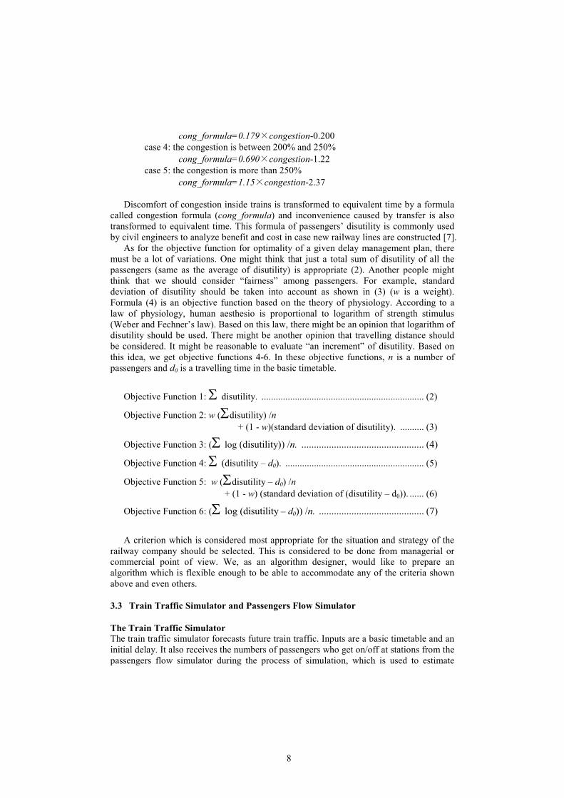
Discomfort of congestion inside trains is transformed to equivalent time by a formula

called congestion formula (cong_formula) and inconvenience caused by transfer is also

transformed to equivalent time. This formula of passengers’ disutility is commonly used

by civil engineers to analyze benefit and cost in case new railway lines are constructed [7].

As for the objective function for optimality of a given delay management plan, there

must be a lot of variations. One might think that just a total sum of disutility of all the

passengers (same as the average of disutility) is appropriate (2). Another people might

think that we should consider “fairness” among passengers. For example, standard

deviation of disutility should be taken into account as shown in (3) (w is a weight).

Formula (4) is an objective function based on the theory of physiology. According to a

law of physiology, human aesthesio is proportional to logarithm of strength stimulus

(Weber and Fechner’s law). Based on this law, there might be an opinion that logarithm of

disutility should be used. There might be another opinion that travelling distance should

be considered. It might be reasonable to evaluate “an increment” of disutility. Based on

this idea, we get objective functions 4-6. In these objective functions, n is a number of

passengers and d0 is a travelling time in the basic timetable.

Objective Function 1: Σ disutility. .................................................................... (2)

Objective Function 2: w (Σdisutility) /n

+ (1 - w)(standard deviation of disutility). .......... (3)

Objective Function 3: (Σ log (disutility)) /n. ................................................. (4)

Objective Function 4: Σ (disutility – d0). .......................................................... (5)

Objective Function 5: w (Σdisutility – d0) /n

+ (1 - w) (standard deviation of (disutility – d0)). ...... (6)

Objective Function 6: (Σ log (disutility – d0)) /n. .......................................... (7)

A criterion which is considered most appropriate for the situation and strategy of the

railway company should be selected. This is considered to be done from managerial or

commercial point of view. We, as an algorithm designer, would like to prepare an

algorithm which is flexible enough to be able to accommodate any of the criteria shown

above and even others.

3.3 Train Traffic Simulator and Passengers Flow Simulator

The Train Traffic Simulator

The train traffic simulator forecasts future train traffic. Inputs are a basic timetable and an

initial delay. It also receives the numbers of passengers who get on/off at stations from the

passengers flow simulator during the process of simulation, which is used to estimate

9

necessary dwell time.

We adopt PERT (Program Evaluation and Review Technique) based simulation

method which has a characteristic that the simulation speed is very high. This technique

was used to develop an efficient train rescheduling algorithm focusing on critical paths

[11].

Train timetable is expressed by a PERT network, in which nodes correspond to events

(arrival or departure of trains) and arcs correspond to chronological dependencies and

minimum required time between two events. There are nine types of arcs as shown in

Table 1. In urban areas of Japan, timetables are usually made with a unit of 5 seconds

(sometimes 10 seconds or 15 seconds) and weights of Table 1 is also specified with the

same time unit.

The weight given to a Train arc is a minimum running time specified in advance. This

minimum running time does not contain margin, because we assume if a train is delayed,

the train runs as fast as possible (but trains never arrive earlier than the planned arrival

time because there is a scheduled arc to the arrival node whose weight is a planned arrival

time.

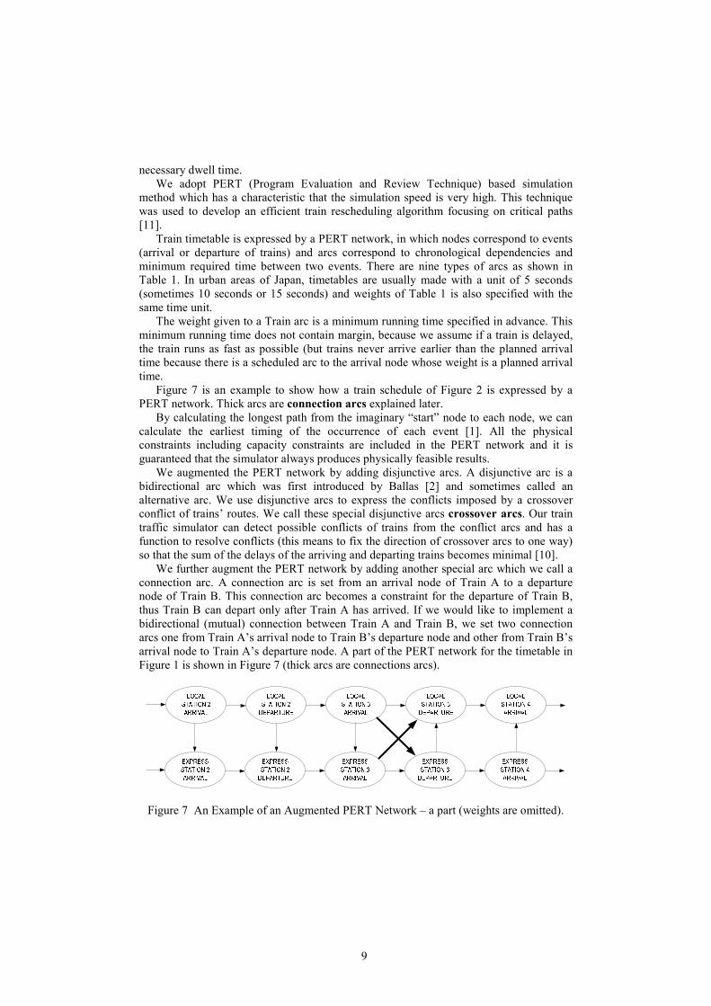
Figure 7 is an example to show how a train schedule of Figure 2 is expressed by a

PERT network. Thick arcs are connection arcs explained later.

By calculating the longest path from the imaginary “start” node to each node, we can

calculate the earliest timing of the occurrence of each event [1]. All the physical

constraints including capacity constraints are included in the PERT network and it is

guaranteed that the simulator always produces physically feasible results.

We augmented the PERT network by adding disjunctive arcs. A disjunctive arc is a

bidirectional arc which was first introduced by Ballas [2] and sometimes called an

alternative arc. We use disjunctive arcs to express the conflicts imposed by a crossover

conflict of trains’ routes. We call these special disjunctive arcs crossover arcs. Our train

traffic simulator can detect possible conflicts of trains from the conflict arcs and has a

function to resolve conflicts (this means to fix the direction of crossover arcs to one way)

so that the sum of the delays of the arriving and departing trains becomes minimal [10].

We further augment the PERT network by adding another special arc which we call a

connection arc. A connection arc is set from an arrival node of Train A to a departure

node of Train B. This connection arc becomes a constraint for the departure of Train B,

thus Train B can depart only after Train A has arrived. If we would like to implement a

bidirectional (mutual) connection between Train A and Train B, we set two connection

arcs one from Train A’s arrival node to Train B’s departure node and other from Train B’s

arrival node to Train A’s departure node. A part of the PERT network for the timetable in

Figure 1 is shown in Figure 7 (thick arcs are connections arcs).

Figure 7 An Example of an Augmented PERT Network – a part (weights are omitted).

10

The Passengers Flow Simulator

This simulator traces passengers from their arrival at their origin station to their

destination station. Thus, we assume that we can obtain OD (origin destination) data of

passengers.

In this paper, a passenger’s behaviour means which train he/she gets on and where

he/she changes trains.

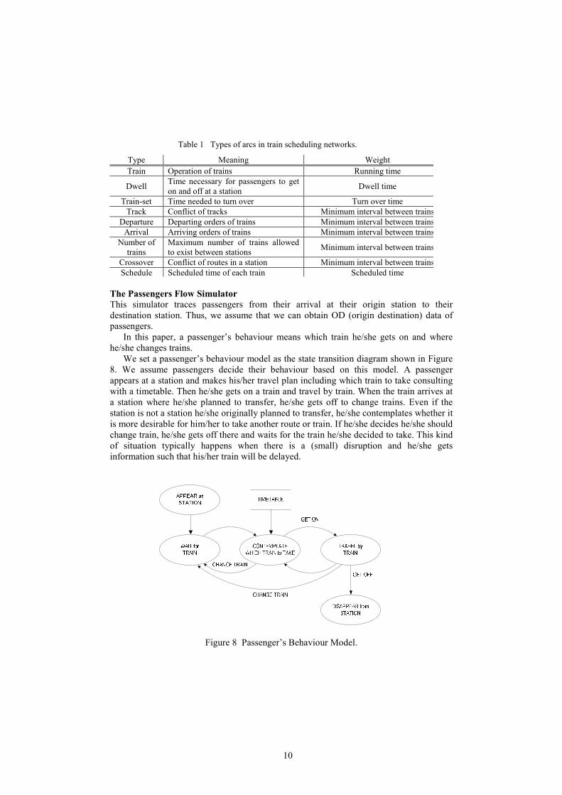
We set a passenger’s behaviour model as the state transition diagram shown in Figure

8. We assume passengers decide their behaviour based on this model. A passenger

appears at a station and makes his/her travel plan including which train to take consulting

with a timetable. Then he/she gets on a train and travel by train. When the train arrives at

a station where he/she planned to transfer, he/she gets off to change trains. Even if the

station is not a station he/she originally planned to transfer, he/she contemplates whether it

is more desirable for him/her to take another route or train. If he/she decides he/she should

change train, he/she gets off there and waits for the train he/she decided to take. This kind

of situation typically happens when there is a (small) disruption and he/she gets

information such that his/her train will be delayed.

Figure 8 Passenger’s Behaviour Model.

Table 1 Types of arcs in train scheduling networks.

Type Meaning Weight

Train Operation of trains Running time

Dwell Time necessary for passengers to get

on and off at a station Dwell time

Train-set Time needed to turn over Turn over time

Track Conflict of tracks Minimum interval between trains

Departure Departing orders of trains Minimum interval between trains

Arrival Arriving orders of trains Minimum interval between trains

Number of

trains

Maximum number of trains allowed

to exist between stations Minimum interval between trains

Crossover Conflict of routes in a station Minimum interval between trains

Schedule Scheduled time of each train Scheduled time

11

Please note that the timetable information in Figure 8 is not always the same as the

basic timetable. “Timetable” in Figure 8 is actually timetable information that each

passenger has in his/her mind. In other words, if a passenger has received announcement

about delays of trains as explained above, the timetable information is modified reflecting

the announcement. During the process of simulation, the timetable information is

modified considering what kind of information is given to passengers. One extreme is to

prepare different timetable information for each passenger, reflecting the information

he/she has received and knowledge about timetable and railway network and so on.

Modification of the timetable is conducted by calling the train traffic simulator as depicted

in Figure 6.

This behaviour model makes the following possible:

1. Passengers usually take a route they first selected when they arrive at a station,

but if there is a change of situation, they may change their route. For example, if

they get announcement of a better route in case of disruption or if a train has

become more congested than expected, passengers may change their routes.

2. It is obvious that passengers cannot take action forecasting the future. For

example, if a passenger knows in advance that a train is delayed, he/she does not

take the train. But this is not reasonable. In other words, passengers flow

simulator has to have ability to prohibit passengers to forecast the future. If there

exists only one timetable information, eg. only a rescheduled timetable is prepared

and if passengers decide their behaviour based on this timetable information, this

means that passengers can forecast the future. We have solved this problem by

switching the timetable information when necessary.

We assume that passengers decide their route (including selection of trains) so that

their disutility becomes minimum. In order to find such a route, we use the following

procedure.

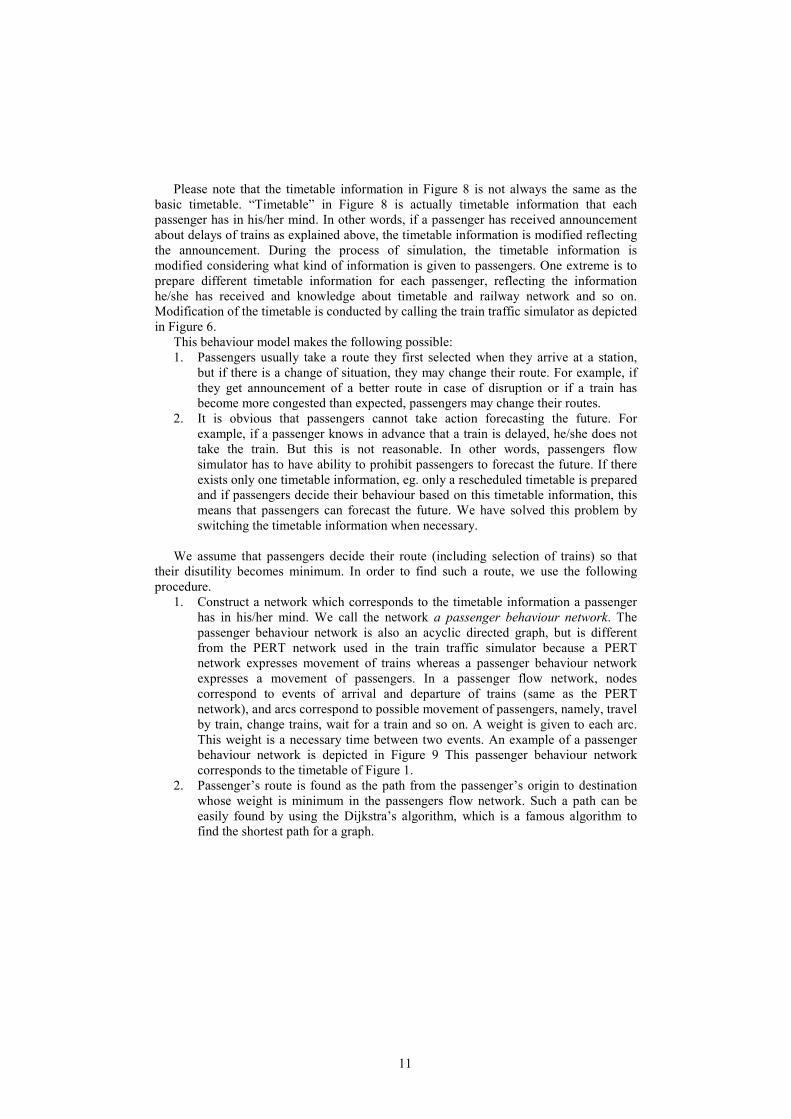
1. Construct a network which corresponds to the timetable information a passenger

has in his/her mind. We call the network a passenger behaviour network. The

passenger behaviour network is also an acyclic directed graph, but is different

from the PERT network used in the train traffic simulator because a PERT

network expresses movement of trains whereas a passenger behaviour network

expresses a movement of passengers. In a passenger flow network, nodes

correspond to events of arrival and departure of trains (same as the PERT

network), and arcs correspond to possible movement of passengers, namely, travel

by train, change trains, wait for a train and so on. A weight is given to each arc.

This weight is a necessary time between two events. An example of a passenger

behaviour network is depicted in Figure 9 This passenger behaviour network

corresponds to the timetable of Figure 1.

2. Passenger’s route is found as the path from the passenger’s origin to destination

whose weight is minimum in the passengers flow network. Such a path can be

easily found by using the Dijkstra’s algorithm, which is a famous algorithm to

find the shortest path for a graph.

12

Figure 9 An Example of a Passenger Behaviour Network – a part (weights are omitted).

Coordination between two simulators

Coordination between the train traffic simulator and the passenger flow simulator is

realized as follows.

1. A PERT network is constructed from the basic timetable and the initial delay.

2. A topological ordering [5] is done to the PERT network.

3. The longest distance of each node from the imaginary start node (this means the

earliest time the event can occur) is calculated following the topological order. If

the node is a departure node, calculation is temporarily suspended and the control

is handed to the passengers flow simulator.

4. The passengers flow simulator calculates how many passengers get on/off at the

station. This calculation is done based on estimation of each passenger’s selection

of routes, namely by finding the shortest path in the passengers flow network for

each passenger.

5. The number of passengers who get on/off at the station is given to the train traffic

simulator and the necessary dwell time is calculated by the following formula. x is

the number of passengers who get on/off at the most congested door of the train.

This formula was obtained empirically for standard commuting trains [12]. Please

note that in Japan, most of the commuting trains are mono-class and the train class

is not considered in this formula.

max(21.9 log(x) – 37.1, minimum dwell time) ............................................ (8)

3.4 Optimization by Tabu Search

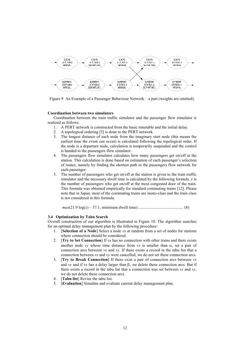
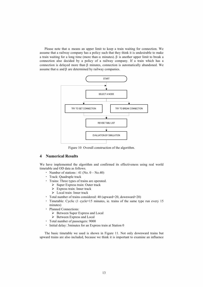
Overall construction of our algorithm is illustrated in Figure 10. The algorithm searches

for an optimal delay management plan by the following procedure:

1. [Selection of a Node] Select a node vx at random from a set of nodes for stations

where connection should be considered.

2. [Try to Set Connection] If vx has no connection with other trains and there exists

another node vy whose time distance from vx is smaller than α, set a pair of

connection arcs between vx and vy. If there exists a record in the tabu list that a

connection between vx and vy were cancelled, we do not set these connection arcs.

3. [Try to Break Connection] If there exist a pair of connection arcs between vx

and vy and if vx has a delay larger than β, we delete these connection arcs. But if

there exists a record in the tabu list that a connection was set between vx and vy,

we do not delete these connection arcs.

4. [Tabu list] Revise the tabu list.

5. [Evaluation] Simulate and evaluate current delay management plan.

13

Please note that α means an upper limit to keep a train waiting for connection. We

assume that a railway company has a policy such that they think it is undesirable to make

a train waiting for a long time (more than α minutes). β is another upper limit to break a

connection also decided by a policy of a railway company. If a train which has a

connection is delayed more than β minutes, connection is automatically abandoned. We

assume that α and β are determined by railway companies.

SELECT A NODE

START

TRY TO SET CONNECTION TRY TO BREAK CONNECTION

REVISE TABU LIST

EVALUATION BY SIMULATION

Figure 10 Overall construction of the algorithm.

4 Numerical Results

We have implemented the algorithm and confirmed its effectiveness using real world

timetable and OD data as follows.

・ Number of stations : 41 (No. 0 – No.40)

・ Track: Quadruple track

・ Trains: Three types of trains are operated.

� Super Express train: Outer track

� Express train: Inner track

� Local train: Inner track

・ Total number of trains considered: 40 (upward=20, downward=20)

・ Timetable: Cyclic (1 cycle=15 minutes, ie. trains of the same type run every 15

minutes)

・ Planned Connections:

� Between Super Express and Local

� Between Express and Local

・ Total number of passengers: 9000

・ Initial delay: 3minutes for an Express train at Station 0

The basic timetable we used is shown in Figure 11. Not only downward trains but

upward trains are also included, because we think it is important to examine an influence

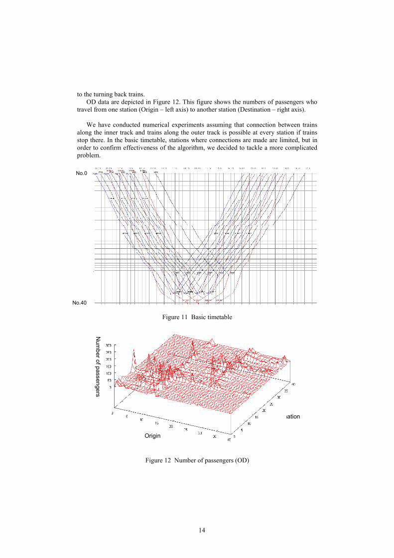
to the turning back trains.

OD data are depicted in Figure 1

travel from one station (Origin

We have conducted numerical experiments assuming that

along the inner track and trains along the outer track is possible at every station

stop there. In the basic timetable

order to confirm effectiveness of the algorithm, we decided to tackle a more complicated

problem.

Number of passengers

No.0

No.40

14

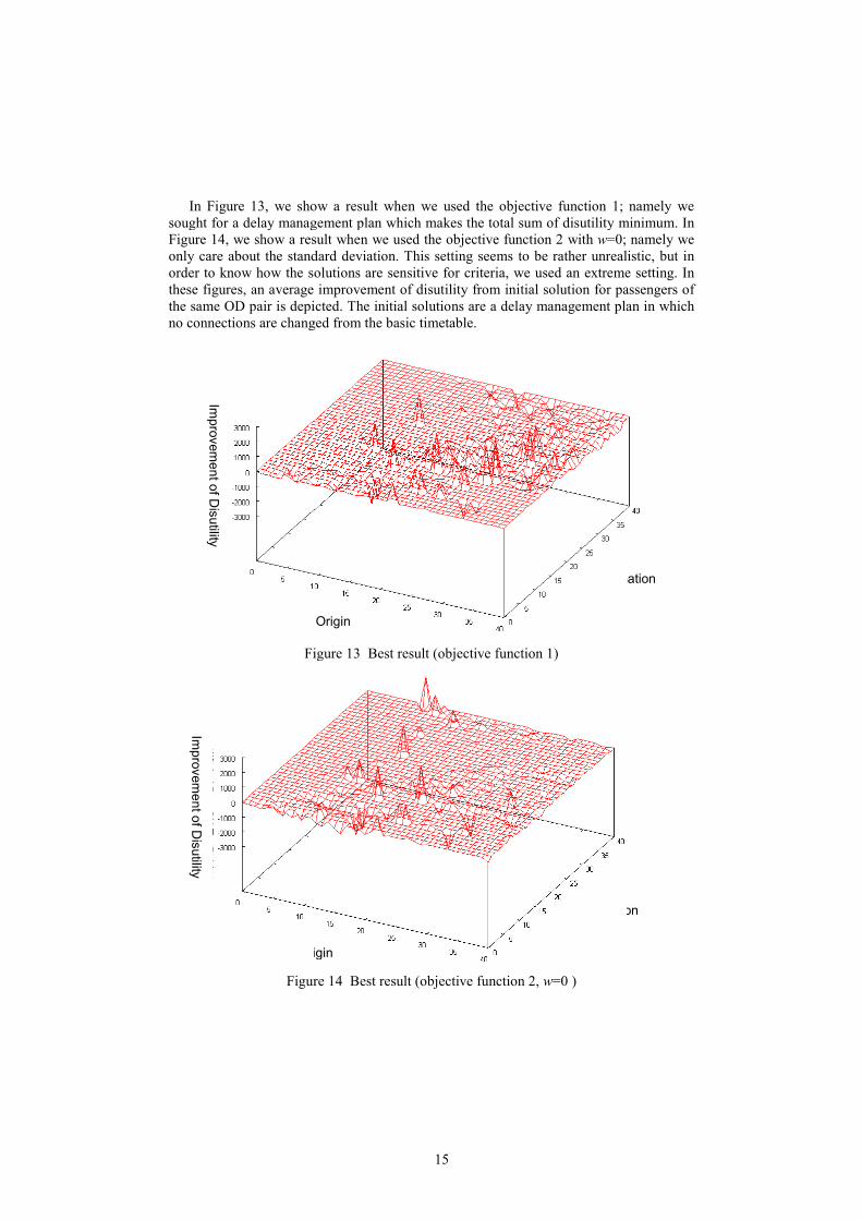
to the turning back trains.

depicted in Figure 12. This figure shows the numbers of passengers who

travel from one station (Origin – left axis) to another station (Destination – right axis).

conducted numerical experiments assuming that connection between trains

along the inner track and trains along the outer track is possible at every station

basic timetable, stations where connections are made are limited, but in


Figure 11 Basic timetable

Figure 12 Number of passengers (OD)

Destination

Origin

of passengers who

right axis).

connection between trains

along the inner track and trains along the outer track is possible at every station if trains

are limited, but in


Destination

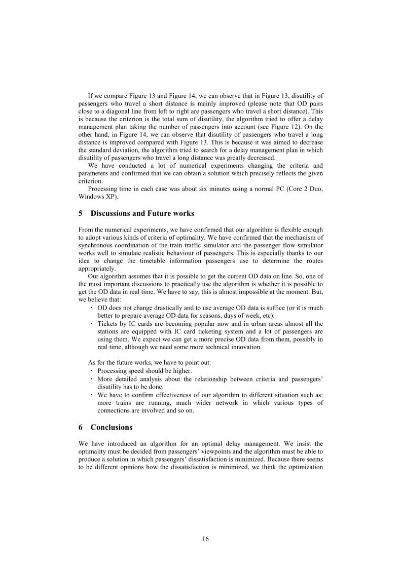
In Figure 13, we show a result when we

sought for a delay management plan which makes the

Figure 14, we show a result when we used

only care about the standard deviation.

order to know how the solutions

these figures, an average

the same OD pair is depicted. The initial solutions are

no connections are changed

Figure 1

Figure 1

Improvement of Disutility

Origin

Improvement of Disutility

15

, we show a result when we used the objective function 1;

sought for a delay management plan which makes the total sum of disutility minimum. In

, we show a result when we used the objective function 2 with w=0;

only care about the standard deviation. This setting seems to be rather unrealistic, but in

order to know how the solutions are sensitive for criteria, we used an extreme

an average improvement of disutility from initial solution for passengers of

picted. The initial solutions are a delay management plan in which

changed from the basic timetable.

Figure 13 Best result (objective function 1)

Figure 14 Best result (objective function 2, w=0 )

Destination

Origin

Destination

Origin

namely we

disutility minimum. In

namely we

rather unrealistic, but in

criteria, we used an extreme setting. In

passengers of

delay management plan in which

Destination

Destination

16

If we compare Figure 13 and Figure 14, we can observe that in Figure 13, disutility of

passengers who travel a short distance is mainly improved (please note that OD pairs

close to a diagonal line from left to right are passengers who travel a short distance). This

is because the criterion is the total sum of disutility, the algorithm tried to offer a delay

management plan taking the number of passengers into account (see Figure 12). On the

other hand, in Figure 14, we can observe that disutility of passengers who travel a long

distance is improved compared with Figure 13. This is because it was aimed to decrease

the standard deviation, the algorithm tried to search for a delay management plan in which

disutility of passengers who travel a long distance was greatly decreased.

We have conducted a lot of numerical experiments changing the criteria and

parameters and confirmed that we can obtain a solution which precisely reflects the given

criterion.

Processing time in each case was about six minutes using a normal PC (Core 2 Duo,

Windows XP).

5 Discussions and Future works

From the numerical experiments, we have confirmed that our algorithm is flexible enough

to adopt various kinds of criteria of optimality. We have confirmed that the mechanism of

synchronous coordination of the train traffic simulator and the passenger flow simulator

works well to simulate realistic behaviour of passengers. This is especially thanks to our

idea to change the timetable information passengers use to determine the routes

appropriately.

Our algorithm assumes that it is possible to get the current OD data on line. So, one of

the most important discussions to practically use the algorithm is whether it is possible to

get the OD data in real time. We have to say, this is almost impossible at the moment. But,

we believe that:

・ OD does not change drastically and to use average OD data is suffice (or it is much

better to prepare average OD data for seasons, days of week, etc).

・ Tickets by IC cards are becoming popular now and in urban areas almost all the

stations are equipped with IC card ticketing system and a lot of passengers are

using them. We expect we can get a more precise OD data from them, possibly in

real time, although we need some more technical innovation.

As for the future works, we have to point out:

・ Processing speed should be higher.

・ More detailed analysis about the relationship between criteria and passengers’

disutility has to be done.

・ We have to confirm effectiveness of our algorithm to different situation such as:

more trains are running, much wider network in which various types of

connections are involved and so on.

6 Conclusions

We have introduced an algorithm for an optimal delay management. We insist the

optimality must be decided from passengers’ viewpoints and the algorithm must be able to

produce a solution in which passengers’ dissatisfaction is minimized. Because there seems

to be different opinions how the dissatisfaction is minimized, we think the optimization

17

algorithm must be flexible enough to adopt various kinds of criteria.

Bearing these requirements in mind, we have developed an algorithm to produce an

optimal delay management plan on line. The algorithm is a combination of simulation and

optimization. Simulation part consists of a train traffic simulator and a passenger flow

simulator which work in parallel.

We have conducted numerical experiments and confirmed that our algorithm is very

promising.

This research was partially supported by the Ministry of Education, Science, Sports

and Culture, Grant-in-Aid for Scientific Research (C) 21510156.

References

[1] Abe, K. and Araya, S. : Train Traffic Simulation Algorithm using Longest Path

Method (in Japanese), Transactions of Information Processing Society of Japan,

Vol.27, No.1, 1986.

[2] Ballas, E. : Machine sequencing via disjunctive graphs: an implicit enumeration

approach, Operations Research, 17, 941-957, 1969.

[3] Dollevoet T., Huisman, D., Schmidt, M. and Shӧbel, A. : Delay Management with

Re-Routing of Passengers, ATMOS 9th Workshop on Algorithmic Approaches for

Transportation Modeling, Optimization and Systems 2009.

[4] Gatto,M., Glaus, B., Jacob, R., Peeters, L. and Widmayer, P. : Railway delay

management: Exploring its algorithmic complexity. In Proc. 9th Scand. Workshop

on Algorithm Theory (SWAT), volume 3111 of LNCS, pages 199-211, 2004.

[5] Jungnickel, D. And Schade, T. : Graphs, Networks & Algorithms, Springer, 2003.

[6] Kunimatsu, T., Hirai, C., Tomii, N. and Takaba, M. : Evaluation of timetables by

estimating passengers' personal disutility using micro-simulation, RailZurich2009 –

3rd International Seminar on Railway Operations Modelling and Analysis, Zurich,

Feb. 2009.

[7] Ministry of Land, Infrastructure, Transport and Tourism of Japan : Evaluation

manual for railway projects 2005 (in Japanese), Institution for Transport Policy

Studies of Japan, 2005.

[8] Schachtebeck, N. and Shӧbel, A.: Algorithms for Delay Management with Capacity

Constraints, ARRIVAL TR-0070, 2007.

[9] Schӧbel, A. : Integer programming approaches for solving the delay management

problem. In Algorithmic Methods for Railway Optimization, Lecture Notes in

Computer Science, Springer, 2007.

[10] Tomii, N. and Ikeda, H. : A Train Traffic Rescheduling Simulator Combining PERT

and Knowledge-Based Approach, ESS'95, European Simulation Symposium,

Elrangen, Germany, Nov. 1995.

[11] Tomii, N., Tashiro, Y., Tanabe, N., Hirai, C., Muraki, K. : Train Rescheduling

Algorithm which minimizes Passengers' Dissatisfaction, in Moonis. Ali et al. eds.,

Innovations in Applied Artificial Intelligence, Lecture Notes in Artificial Intelligence

3533, Springer, 2005.

[12] Toriumi, S., Nakamura, Y., Taguchi, A. : Delay Calculation Model of Commuter

Trains (in Japanese), Communications of Operations Research of Japan, Vol.50,

No.6, pp.409-416, June2005.

an optimal delay management algorithm from passengers ... · an optimal delay management algorithm...

Documents