an introduction to security valuation. the investment decision process determine the required rate...
TRANSCRIPT

An Introduction to Security Valuation

The Investment Decision Process
• Determine the required rate of return
• Evaluate the investment to determine if its market price is consistent with your required rate of return– Estimate the value of the security based on its
expected cash flows and your required rate of return
– Compare this intrinsic value to the market price to decide if you want to buy it
Valuation Process
• Two approaches– 1. Top-down, three-step approach– 2. Bottom-up, stock valuation, stock picking
approach
• The difference between the two approaches is the perceived importance of economic and industry influence on individual firms and stocks

Top-Down, Three-Step Approach
1. General economic influences– Decide how to allocate investment funds among
countries, and within countries to bonds, stocks, and cash
2. Industry influences– Determine which industries will prosper and which
industries will suffer on a global basis and within countries
3. Company analysis– Determine which companies in the selected industries
will prosper and which stocks are undervalued
Does the Three-Step Process Work?
• Studies indicate that most changes in an individual firm’s earnings can be attributed to changes in aggregate corporate earnings and changes in the firm’s industry

Does the Three-Step Process Work?
• Studies have found a relationship between aggregate stock prices and various economic series such as employment, income, or production

Does the Three-Step Process Work?
• An analysis of the relationship between rates of return for the aggregate stock market, alternative industries, and individual stocks showed that most of the changes in rates of return for individual stock could be explained by changes in the rates of return for the aggregate stock market and the stock’s industry

Theory of Valuation
• The value of an asset is the present value of its expected returns
• You expect an asset to provide a stream of returns while you own it

Theory of Valuation
• To convert this stream of returns to a value for the security, you must discount this stream at your required rate of return
• This requires estimates of:– The stream of expected returns, and– The required rate of return on the investment

Stream of Expected Returns
• Form of returns– Earnings– Cash flows– Dividends– Interest payments– Capital gains (increases in value)
• Time pattern and growth rate of returns
Required Rate of Return
• Determined by– 1. Economy’s risk-free rate of return, plus– 2. Expected rate of inflation during the holding
period, plus– 3. Risk premium determined by the
uncertainty of returns

Investment Decision Process: A Comparison of Estimated Values and
Market Prices
If Estimated Value > Market Price, Buy
If Estimated Value < Market Price, Don’t Buy

Valuation of Alternative Investments
• Valuation of Bonds is relatively easy because the size and time pattern of cash flows from the bond over its life are known
1. Interest payments are made usually every six months equal to one-half the coupon rate times the face value of the bond
2. The principal is repaid on the bond’s maturity date

Valuation of Bonds
• Example: in 2002, a $10,000 bond due in 2017 with 10% coupon
• Discount these payments at the investor’s required rate of return (if the risk-free rate is 9% and the investor requires a risk premium of 1%, then the required rate of return would be 10%)

Valuation of Bonds
Present value of the interest payments is an annuity for thirty periods at one-half the required rate of return:
$500 x 15.3725 = $7,686
The present value of the principal is similarly discounted:
$10,000 x .2314 = $2,314
Total value of bond at 10 percent = $10,000

Valuation of Bonds
The $10,000 valuation is the amount that an investor should be willing to pay for this bond, assuming that the required rate of return on a bond of this risk class is 10 percent

Valuation of Bonds
If the market price of the bond is above this value, the investor should not buy it because the promised yield to maturity will be less than the investor’s required rate of return

Valuation of Bonds
Alternatively, assuming an investor requires a 12 percent return on this bond, its value would be:
$500 x 13.7648 = $6,882
$10,000 x .1741 = 1,741
Total value of bond at 12 percent = $8,623
Higher rates of return lower the value!
Compare the computed value to the market price of the bond to determine whether you should buy it.

Valuation of Preferred Stock
• Owner of preferred stock receives a promise to pay a stated dividend, usually quarterly, for perpetuity
• Since payments are only made after the firm meets its bond interest payments, there is more uncertainty of returns
• Tax treatment of dividends paid to corporations (80% tax-exempt) offsets the risk premium
Valuation of Preferred Stock
pk
DividendV
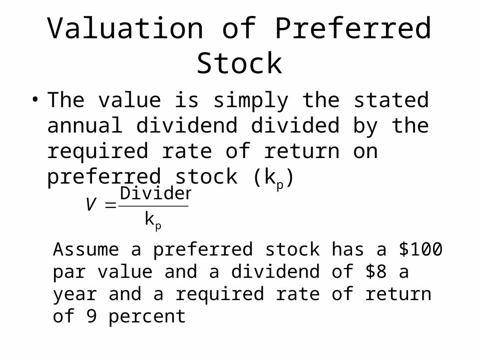
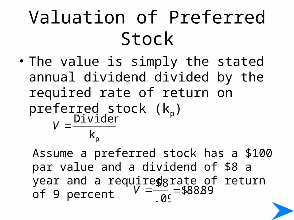
• The value is simply the stated annual dividend divided by the required rate of return on preferred stock (kp)
Assume a preferred stock has a $100 par value and a dividend of $8 a year and a required rate of return of 9 percent
Valuation of Preferred Stock
pk
DividendV
• The value is simply the stated annual dividend divided by the required rate of return on preferred stock (kp)
Assume a preferred stock has a $100 par value and a dividend of $8 a year and a required rate of return of 9 percent
.09
$8V 89.88$

Valuation of Preferred Stock
Given a market price, you can derive its promised yield
At a market price of $85, this preferred stock yield would be
Price
Dividendk p
0941.$85.00
$8k p

Approaches to the Valuation of Common Stock
Two approaches have developed1. Discounted cash-flow valuation
• Present value of some measure of cash flow, including dividends, operating cash flow, and free cash flow
2. Relative valuation technique• Value estimated based on its price relative to
significant variables, such as earnings, cash flow, book value, or sales
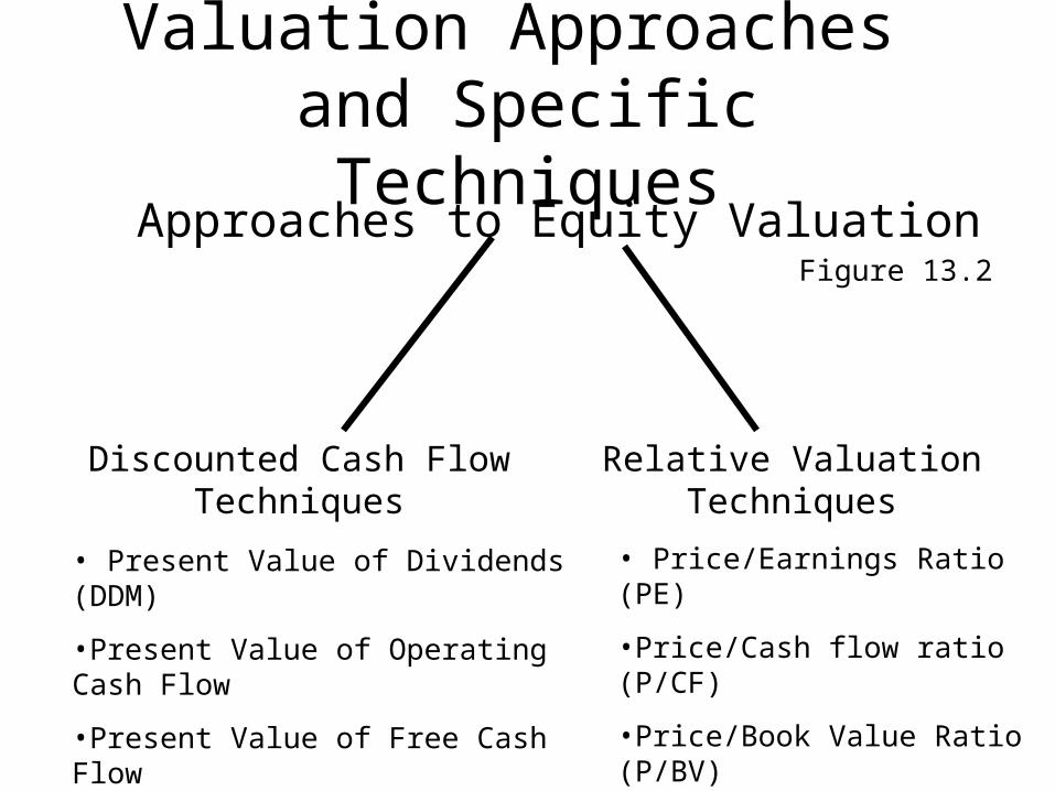
Valuation Approaches and Specific Techniques
Approaches to Equity Valuation
Discounted Cash Flow Techniques
Relative Valuation Techniques
• Present Value of Dividends (DDM)
•Present Value of Operating Cash Flow
•Present Value of Free Cash Flow
• Price/Earnings Ratio (PE)
•Price/Cash flow ratio (P/CF)
•Price/Book Value Ratio (P/BV)
•Price/Sales Ratio (P/S)
Figure 13.2

Approaches to the Valuation of Common Stock
The discounted cash flow approaches are dependent on some factors, namely:• The rate of growth and the duration of growth
of the cash flows• The estimate of the discount rate

Why and When to Use the Discounted Cash Flow Valuation
Approach• The measure of cash flow used– Dividends
• Cost of equity as the discount rate
– Operating cash flow• Weighted Average Cost of Capital (WACC)
– Free cash flow to equity• Cost of equity
• Dependent on growth rates and discount rate
Why and When to Use the Relative Valuation Techniques
• Provides information about how the market is currently valuing stocks– aggregate market– alternative industries– individual stocks within industries
• No guidance as to whether valuations are appropriate– best used when have comparable entities– aggregate market is not at a valuation extreme

Discounted Cash-Flow Valuation Techniques
nt
tt
tj k
CFV
1 )1( Where:
Vj = value of stock j
n = life of the asset
CFt = cash flow in period t
k = the discount rate that is equal to the investor’s required rate of return for asset j, which is determined by the uncertainty (risk) of the stock’s cash flows
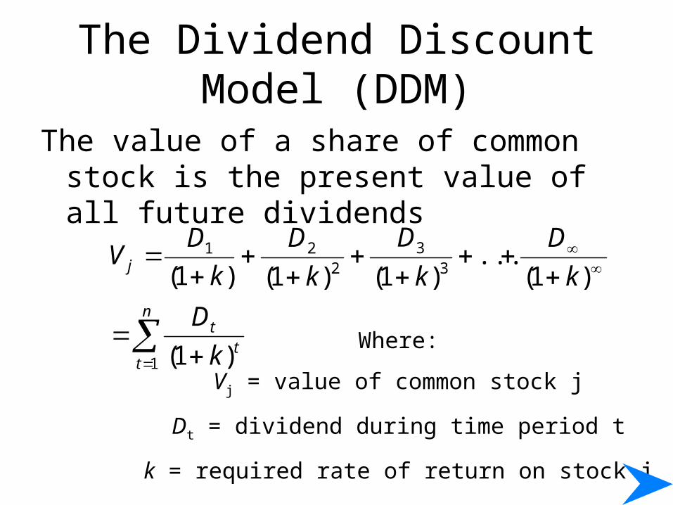
The Dividend Discount Model (DDM)
The value of a share of common stock is the present value of all future dividends
n
tt
t
j
k
D
k
D
k
D
k
D
k
DV
1
33
221
)1(
)1(...
)1()1()1(
Where:
Vj = value of common stock j
Dt = dividend during time period t
k = required rate of return on stock j

The Dividend Discount Model (DDM)
If the stock is not held for an infinite period, a sale at the end of year 2 would imply:
Selling price at the end of year two is the value of all remaining dividend payments, which is simply an extension of the original equation
2
2
221
)1()1()1( k
SP
k
D
k
DV jj

The Dividend Discount Model (DDM)
Stocks with no dividends are expected to start paying dividends at some point, say year three...
Where:
D1 = 0
D2 = 0
)1(...
)1()1()1( 33
221
k
D
k
D
k
D
k
DV j

The Dividend Discount Model (DDM)
Infinite period model assumes a constant growth rate for estimating future dividends
Where:
Vj = value of stock j
D0 = dividend payment in the current period
g = the constant growth rate of dividends
k = required rate of return on stock j
n = the number of periods, which we assume to be infinite
n
n
j k
gD
k
gD
k
gDV
)1(
)1(...
)1(
)1(
)1(
)1( 02
200

The Dividend Discount Model (DDM)
Infinite period model assumes a constant growth rate for estimating future dividends
This can be reduced to:
1. Estimate the required rate of return (k)
2. Estimate the dividend growth rate (g)
n
n
j k
gD
k
gD
k
gDV
)1(
)1(...
)1(
)1(
)1(
)1( 02
200
gk
DV j
1

Infinite Period DDM and Growth Companies
Assumptions of DDM:
1. Dividends grow at a constant rate
2. The constant growth rate will continue for an infinite period
3. The required rate of return (k) is greater than the infinite growth rate (g)

Infinite Period DDM and Growth Companies
Growth companies have opportunities to earn return on investments greater than their required rates of return
To exploit these opportunities, these firms generally retain a high percentage of earnings for reinvestment, and their earnings grow faster than those of a typical firm
This is inconsistent with the infinite period DDM assumptions

Infinite Period DDM and Growth Companies
The infinite period DDM assumes constant growth for an infinite period, but abnormally high growth usually cannot be maintained indefinitely
Risk and growth are not necessarily related
Temporary conditions of high growth cannot be valued using DDM

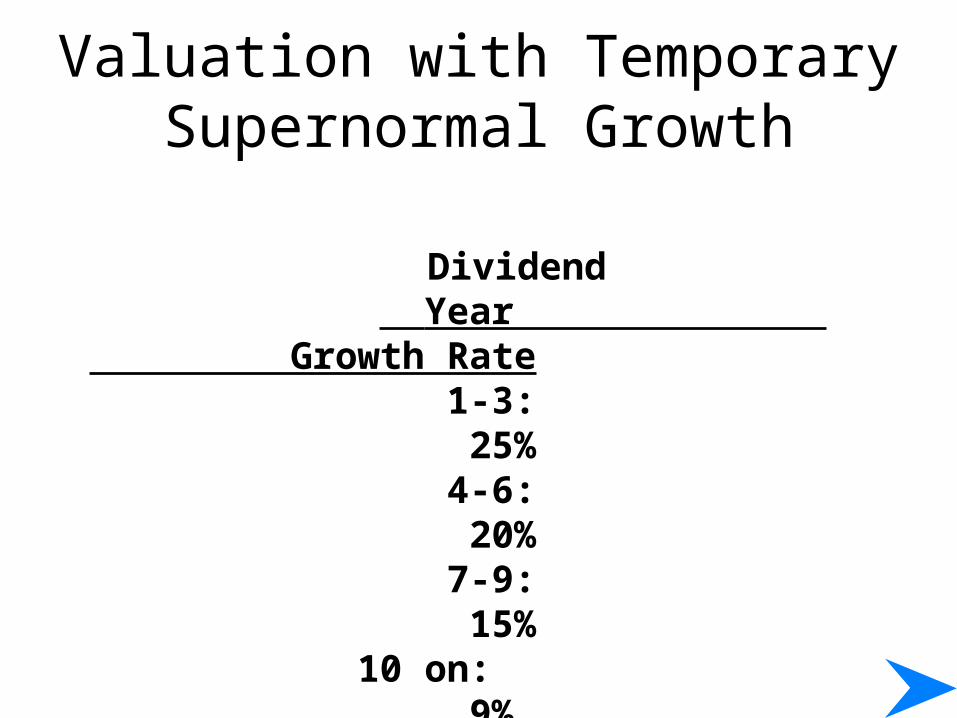
Valuation with Temporary Supernormal Growth
Combine the models to evaluate the years of supernormal growth and then use DDM to compute the remaining years at a sustainable rate
For example:
With a 14 percent required rate of return and dividend growth of:
Valuation with Temporary Supernormal Growth
Dividend Year Growth Rate 1-3: 25% 4-6: 20% 7-9: 15% 10 on: 9%

Valuation with Temporary Supernormal Growth
The value equation becomes
9
333
9
333
8
233
7
33
6
33
5
23
4
3
3
3
2
2
)14.1(
)09.14(.
)09.1()15.1()20.1()25.1(00.2
14.1
)15.1()20.1()25.1(00.2
14.1
)15.1()20.1()25.1(00.2
14.1
)15.1()20.1()25.1(00.2
14.1
)20.1()25.1(00.2
14.1
)20.1()25.1(00.2
14.1
)20.1()25.1(00.2
14.1
)25.1(00.2
14.1
)25.1(00.2
14.1
)25.1(00.2
iV

Computation of Value for Stock of Company with Temporary Supernormal Growth
Discount Present Growth
Year Dividend Factor Value Rate
1 2.50$ 0.8772 2.193$ 25%2 3.13 0.7695 2.408$ 25%3 3.91 0.6750 2.639$ 25%4 4.69 0.5921 2.777$ 20%5 5.63 0.5194 2.924$ 20%6 6.76 0.4556 3.080$ 20%7 7.77 0.3996 3.105$ 15%8 8.94 0.3506 3.134$ 15%9 10.28 0.3075 3.161$ 15%
10 11.21 9%
224.20$ a 0.3075 b 68.943$
94.365$
aValue of dividend stream for year 10 and all future dividends, that is$11.21/(0.14 - 0.09) = $224.20bThe discount factor is the ninth-year factor because the valuation of theremaining stream is made at the end of Year 9 to reflect the dividend inYear 10 and all future dividends.
Exhibit 11.3

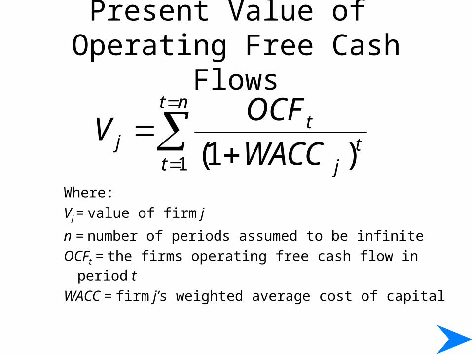
Present Value of Operating Free Cash Flows
• Derive the value of the total firm by discounting the total operating cash flows prior to the payment of interest to the debt-holders
• Then subtract the value of debt to arrive at an estimate of the value of the equity

Present Value of Operating Free Cash Flows
nt
tt
j
tj WACC
OCFV
1 )1(
Present Value of Operating Free Cash Flows
nt
tt
j
tj WACC
OCFV
1 )1(Where:
Vj = value of firm j
n = number of periods assumed to be infinite
OCFt = the firms operating free cash flow in period t
WACC = firm j’s weighted average cost of capital

Present Value of Operating Free Cash Flows
Similar to DDM, this model can be used to estimate an infinite period
Where growth has matured to a stable rate, the adaptation is
OCFjj gWACC
OCFV
1
Where:
OCF1=operating free cash flow in period 1
gOCF = long-term constant growth of operating free cash flow

Present Value of Operating Free Cash Flows
• Assuming several different rates of growth for OCF, these estimates can be divided into stages as with the supernormal dividend growth model
• Estimate the rate of growth and the duration of growth for each period

Present Value of Free Cash Flows to Equity
• “Free” cash flows to equity are derived after operating cash flows have been adjusted for debt payments (interest and principle)
• The discount rate used is the firm’s cost of equity (k) rather than WACC

Present Value of Free Cash Flows to Equity
Where:
Vj = Value of the stock of firm j
n = number of periods assumed to be infinite
FCFt = the firm’s free cash flow in period t
K j = the cost of equity
n
tt
j
tj k
FCFV
1 )1(

Relative Valuation Techniques
• Value can be determined by comparing to similar stocks based on relative ratios
• Relevant variables include earnings, cash flow, book value, and sales
• The most popular relative valuation technique is based on price to earnings

Earnings Multiplier Model
• This values the stock based on expected annual earnings
• The price earnings (P/E) ratio, or
Earnings Multiplier
EarningsMonth -Twelve Expected
PriceMarket Current

Earnings Multiplier Model
The infinite-period dividend discount model indicates the variables that should determine the value of the P/E ratio
Dividing both sides by expected earnings during the next 12 months (E1)
gk
DPi
1
gk
ED
E
Pi
11
1
/
Earnings Multiplier Model
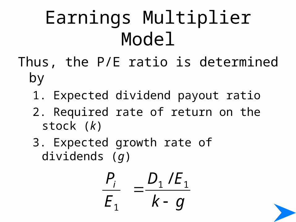
Thus, the P/E ratio is determined by1. Expected dividend payout ratio
2. Required rate of return on the stock (k)
3. Expected growth rate of dividends (g)
gk
ED
E
Pi
11
1
/

Earnings Multiplier Model
As an example, assume:– Dividend payout = 50%– Required return = 12%– Expected growth = 8%– D/E = .50; k = .12; g=.08
12.5
.50/.04
.08-.12
.50P/E

Earnings Multiplier Model
A small change in either or both k or g will have a large impact on the multiplier
gk
ED
E
Pi
11
1
/

Earnings Multiplier Model
A small change in either or both k or g will have a large impact on the multiplier
D/E = .50; k=.13; g=.08 P/E = 10
D/E = .50; k=.12; g=.09 P/E = 16.7
D/E = .50; k=.11; g=.09 P/E = 25
gk
ED
E
Pi
11
1
/

Earnings Multiplier Model
Given current earnings of $2.00 and growth of 9%
You would expect E1 to be $2.18
D/E = .50; k=.12; g=.09 P/E = 16.7
V = 16.7 x $2.18 = $36.41
Compare this estimated value to market price to decide if you should invest in it

The Price-Cash Flow Ratio
• Companies can manipulate earnings
• Cash-flow is less prone to manipulation
• Cash-flow is important for fundamental valuation and in credit analysis

The Price-Cash Flow Ratio
• Companies can manipulate earnings
• Cash-flow is less prone to manipulation
• Cash-flow is important for fundamental valuation and in credit analysis
1
/
t
ti CF
PCFP
Where:P/CFj = the price/cash flow ratio for firm jPt = the price of the stock in period tCFt+1 = expected cash low per share for firm j

The Price-Book Value Ratio
Widely used to measure bank values (most bank assets are liquid (bonds and commercial loans)

The Price-Book Value Ratio
Where:
P/BVj = the price/book value for firm j
Pt = the end of year stock price for firm j
BVt+1 = the estimated end of year book value per share for firm j
1
/
t
tj BV
PBVP

The Price-Sales Ratio
• Strong, consistent growth rate is a requirement of a growth company
• Sales is subject to less manipulation than other financial data

The Price-Sales Ratio
Where: 1
t
t
S
P
S
P
tjS
jP
jS
P
t
t
j
j
Year during firmfor shareper sales annual
firmfor pricestock year of end
firmfor ratio sales toprice
1

Estimating the Inputs: The Required Rate of Return and The Expected
Growth Rate of Valuation Variables
Valuation procedure is the same for securities around the world, but the required rate of return (k) and expected growth rate of earnings and other valuation variables (g) such as book value, cash flow, and dividends differ among countries

Required Rate of Return (k)
The investor’s required rate of return must be estimated regardless of the approach selected or technique applied
• This will be used as the discount rate and also affects relative-valuation
• This is not used for present value of free cash flow which uses the required rate of return on equity (K)
• It is also not used in present value of operating cash flow which uses WACC

Required Rate of Return (k)
Three factors influence an investor’s required rate of return:
• The economy’s real risk-free rate (RRFR)• The expected rate of inflation (I)• A risk premium (RP)

The Economy’s Real Risk-Free Rate
• Minimum rate an investor should require
• Depends on the real growth rate of the economy– (Capital invested should grow as fast as the
economy)
• Rate is affected for short periods by tightness or ease of credit markets
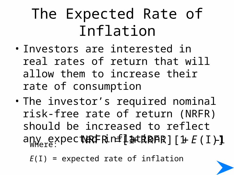
The Expected Rate of Inflation
• Investors are interested in real rates of return that will allow them to increase their rate of consumption
• The investor’s required nominal risk-free rate of return (NRFR) should be increased to reflect any expected inflation:
1-(I)]RRFR][1[1NRFR EWhere:
E(I) = expected rate of inflation

The Risk Premium
• Causes differences in required rates of return on alternative investments
• Explains the difference in expected returns among securities
• Changes over time, both in yield spread and ratios of yields

Risk Premium
• Must be derived for each investment in each country
• The five risk components vary between countries

Risk Components
• Business risk
• Financial risk
• Liquidity risk
• Exchange rate risk
• Country risk

Expected Growth Rate of Dividends• Determined by
– the growth of earnings– the proportion of earnings paid in dividends
• In the short run, dividends can grow at a different rate than earnings due to changes in the payout ratio
• Earnings growth is also affected by compounding of earnings retention
g = (Retention Rate) x (Return on Equity)
= RR x ROE