AN INTRODUCTION TO RISK AND RETURN

CONCEPTS AND EVIDENCE

by

Franco Modigliani and Gerald A. Pogue

646-73

March 1973

Q1LPr�-·I-- -·---?�---�----_I��_�� _��_ ��� �__�___���

AN INTRODUCTION TO RISK AND RETURN

CONCEPTS AND EVIDENCE

by

Franco Modigliani and Gerald A. Pogue1

Today, most students of financial management would agree that

the treatment of risk is the main element in financial decision making.

Key current questions involve how risk should be measured, and how the

required return associated with a given risk level is determined. A

large body of literature has developed in an attempt to answer these

questions.

However, risk did not always have such a prominent place.

Prior to 1952 the risk element was usually either assumed away or

treated qualitatively in the financial literature. In 1952 an event occurred

which was to revolutionize the theory of financial management. In a

path-breaking article, an economist by the name of Harry Markowitz [ 17]

suggested a powerful yet simple approach for dealing with risk. In the

two decades since, the modern theory of portfolio management has

evolved.

Portfolio theory deals with the measurement of risk, and the

relationship between risk and return. It is concerned with the impli-ca-

tions for security prices of the portfolio decisions made by investors.

If, for example, all investors select stocks to maximize expected

portfolio return for individually acceptable levels of investment risk,

what relationship would result between required returns and risk?

-1-

-�--�-I� -·- --·--- ----iL__i..�_l_��.�_�. ...

One answer to this question has been developed by Professors

Lintner [ 14, 15] and Sharpe [22], called the Capital Asset Pricing Model.

Once such a normative relationship between risk and return is obtained,

it has an obvious application as a benchmark for evaluating the performance

of managed portfolios.

The purpose of this paper is to present a nontechnical introduction

to modern portfolio theory. Our hope is to provide a wide class of

readers with an understanding of the foundations upon which risk measures

such as "beta", for example, are based. We will present the main

elements of the theory along with the results of some of the more important

empirical tests. We are not attempting to present an exhaustive survey

of the theoretical and empirical literature.

The paper is organized as follows. Section 1 develops measures

of investment return which are used in the study. Section 2 introduces

the concept of portfolio risk. We will suggest, as did H. Harkowitz in

1952, that the standard deviation of portfolio returns be used as a measure

of total portfolio risk. Section 3 deals with the impact of diversification

on portfolio risk. The concepts of systematic and unsystematic risk are

introduced here. Section 4 deals with the contribution of individual

securities to portfolio risk. The nondiversifiable or systematic risk of a

portfolio is shown to be a weighted average of the systematic risk of its

component securities. Section 5 discusses procedures for measuring

the systematic risk or "beta" factors for securities and portfolios.

Section 6 presents an intuitive justification of the capital asset pricing

model. This model provides a normative relationship between security

risk and expected return. Section 7 presents a review of empirical

tests of the model. The purpose of these tests is to see how well the

-2-

model explains the relationship between risk and return that exists in

the securities market. Finally, Section 8 discusses how we can use the

capital asset pricing model to measure the performance of institutional

investors.

-3-

~~~1_ __~~~~~~~~_1 ~ ~ ~ ~ ~ ~ --·-- 11 ~ ~ ~ ~ ~ ~ ~ ~ ~ ~ ~ ~ ~ ~ 1-1_1~~~~~~------ -----s�-----·-·-��--��.�-�-�

1. INVESTMENT RETURN

Measuring historical rates of return is a relatively straight-

forward matter. The return on our investor's portfolio during some

interval is equal to the capital gains plus any distributions received on

the portfolio. It is important that distributions, such as dividends, be

included, else the measure of return to the investor is deficient. The

return on the investor' s portfolio, designated Rp, is given by

D + AVR = p P (1)R p

Vp

where

· -~ D = dividends receivedP

A V =change in portfolio value during the

interval (Capital Gains)

V market value of the portfolio at thep

beginning of the period

The formula assumes no capital inflows during the measurement period.

Otherwise the calculation would have to be modified to reflect the

increased investment base. Further, the calculation assumes that any

distributions occur at the end of the period, or that distributions are

held in the form of cash until period end. If the distributions were

invested prior to the end of the interval, the calculation would have to

be modified to consider gains or losses on the amount reinvested.

-4-

�____ _�11�1�_1_·________1_1_�11-���

Thus, given the beginning and ending portfolio values and distri-

butions received, we can measure the investor 's return using

Equation (1). For example, if the investor's portfolio had a market

value of $100 at the beginning of June, produced $10 of dividends, and

had an end-of-month value of $95, the return for the month would be

0. 05 or 5%.

To measure the average return over a series of measurement

intervals, two calculations are commonly used: the "arithmetic average"

and the "geometric average" returns. We will describe each below. To

illustrate the calculations, consider a portfolio with successive annual

returns of -0. 084, 0.040, and 0. 143. Designate these returns as R 1, R 2 ,

and R 3.

The arithmetic return measures the average portfolio return

realized during successive 1-year periods. It is simply any unweighted

average of the three annual returns; that is, (R1 + R 2 + R 3 ) / 3. The

value for the portfolio is 3.3 percent per year.

The geometric average measures the compounded rate of growth

of the portfolio over the 3-year period. The average is obtained by taking

a "geometric" average of the three annual returns; that is,

{[(1+ R)(1 + R 2 ) (1+ 3 )] 1/- 1.0 . The resulting growth rate for

the portfolio is 2.9% per annum compounded annually, for a total 3-year

return of 8.9%3.

The geometric average measures the true rate of return while

the arithmetic average is simply an average of successive period returns.

The distinction can perhaps be made clear by an example. Consider an

asset which is purchased for $100 at the beginning of year 1. Suppose the

-5-

_____1_�1___ �__ 1___1__1111111_______ _.---_�II__� .

assets price rises to $200 at the end of the first year and then falls

back to $100 by the end of the second year. The arithmetic average

rate of return is the average of +100% and -50%, or +25%. But an asset

purchased for $100 and having a value of $100 two years later did not '

earn 25%; it clearly earned a zero return. The arithmetic average of

successive one-period returns is obviously not equal to the true rate of

return. The true rate of return is given by the geometric mean return

defined above; that is, [(2.0) (0.5)] -1.0 = 0.

In the remainder of the paper, we will refer to both types of

averages.

-6-

2. PORTFOLIO RISK

The definition of investment risk leads us into much less well

explored territory. Not everyone agrees on how to define risk, let alone

measure it. Nevertheless, there are some attributes of risk which are

reasonably well accepted.

If an investor holds a portfolio of treasury bonds, he faces no

uncertainty about monetary outcome. The value of the portfolio at

maturity of the notes will be identical with the predicted value. The

investor has borne no risk. However, if he has a portfolio composed

of common stocks, it will be impossible to exactly predict the value of

the portfolio as of any future date. The best he can do is to make a

best guess or most likely estimate, qualified by statements about the

range and likelihood of other values. In this case, the investor has

borne risk.

A measure of risk is the extent to which the future

portfolio values are likely to diverge from the expected or predicted

value. More specifically, risk for most investors is related to the

chance that future portfolio values will be less than expected. Thus,

if the investor 's portfolio has a current value of $100, 000, at an

expected value of $110, 000 at the end of the next year, he will be

concerned about the probability of achieving values less than $110, 000.

Before proceeding to the quantification of risk, it is convenient

to shift our attention from the terminal value of the portfolio to the

portfolio rate of return, Rp. Since the increase in portfolio value isp

-7-

-- .__.._____1___ 1___ _- -·-~-l__. I_.- --. _·-_- _-

directly related to Rp, this transformation results in no substantive

difference. However, it is convenient for later analysis.

A particularly useful way to quantify the uncertainty about the

portfolio return is to specify the probability associated with each of the

possible future returns. Assume, for example, that an investor has

identified five possible outcomes for his portfolio return during the

next year. Associated with each return is a subjectively determined

probability, or relative chance of occurrence. The five possible

outcomes are:

Possible 1Return Subjective Probability

50% o 0.1

30% 0.2

i0% 0.4

-10% 0.2

-30% 0. 1

1.00

Note that the probabilities sum to 1 so that the actual portfolio return is

confined to take one of the five possible values. Given this probability

distribution, we can measure the expected return and risk for the port-

folio.

The expected return is simply the weighted average of possible

outcomes, where the weights are the relative chances of occurrence.

The expected return on the portfolio is 10%, given by

-8-

5

E(Rp) = 2 Pj R

j=1

= 0.1(50.0) + 0.2(30.0) + 0.4(10.0)

+ 0.2 (-10.0) + 0.2(-30.0)

(2)

where the R.'s are the possible returns and the Pj's the associated

probabilities. (The expected terminal market value of the portfolio is

equal to M 0 (1 + .10), where M0 is the initial value.)

If risk is defined as the chance of loss or achieving returns less

than expected, it would seem to be logical to measure risk by the

dispersion of the possible returns. below the expected value. However,

risk measures based on below-the-mean variability are difficult to work

with, and furthermore are unnecessary as long as the distribution of

future return is reasonably symmetric about its expected values.

Figure 1 shows three probability distributions: the first symmetric,

the second skewed to the left, and the third skewed to the right. The

symmetrical distribution has no skewness. The dispersion of returns on

one side of the expected return is a mirror image of the dispersion on

the other side of the expected return.

Empirical studies of realized rates of return on diversified port-

volios show that skewness is not a significant problem. If the shapes of

historical distributions are indicative of the shapes of future distributions,

then it makes little difference whether we measure variability of returns

on one or both sides of the expected return. Measures of the total

variability of return will be twice as large as measures of the portfolio's

variability below the expected return if its probability distribution is

-9-

1���_11� _1111_1___��_�-- -.

symmetric. Thus, if total variability is used as a risk surrogate, the

risk rankings for a group of portfolios will be the same as when varia-

bility below the expected return is used. It is for this reason that total

variability of returns has been so widely used as a surrogate for risk.

It now remains to develop a specific measure of total variability

of returns. The measures which are most commonly used are the

variance and standard deviation of returns. Measuring risk by standard

deviation and variance is equivalent to defining risk as total variability

of returns about the expected return, or simply, variability of returns.

The variance of return is a weighted sum of the deviations from

the expected return. The variance, designated p for the portfolio in

the previous example is given by

5

P

0.1(50.0- 10.0)2 + 0.2(30.0- 10.0)2

+ 0.4(10.0- 10.0) .2 + 0.2(-10.0- 10.0)2

+ 0.1(-30.0- 10.0)2

- 484 percent squared (3)

The standard deviation is defined as the square root of the variance. It is

equal to 22%. The larger the variance or standard deviation, the greater the

possible dispersion of future realized values around the expected value,

-10-

and the larger the investor's uncertainty. As a rule of thumb, it is often

suggested 'that two-thirds of the possible returns on a portfolio will be

within one standard deviation of return either side of the expected value;

ninety-five percent will lie with plus or minus two standard deviations

of the expected return.

Figure 2 shows the historical return distributions for a diversified

portfolio. The portfolio is composed'of approximately 100 securities,

with each security having equal weight. The month-by-month returns

cover the period from January 1945 to June 1970. Note that the distri-

bution is approximately symmetric, but not exactly. The arithmetic

average return for the 306-month period is 0.91%0 per month. The

standard deviation about this average is 4.45% per month.

Figure 3 gives the same data for a single security, National

Department Stores. The arithmetic average return is 0.81% per month

over the 306-month period. The most interesting aspect, however, is

the standard deviation of month-by-month returns -- 9.02% per month,

more than double that for the diversified portfolio. This result will be

discussed. further in the next section.

Thus far our discussion of portfolio risk has been confined to a

single-period investment horizon such as the next year.. That is, the

portfolio is held unchanged and evaluated at the end of the year. An

obvious question relates to the effect of holding the portfolio for several

periods, such as the next 20 years: will the 1-year risks tend to cancel

out over time? Given the random walk nature of security prices, the

answer to this question is no. If the risk level (standard deviation) is

maintained during each year, the portfolio risk for longer horizons will

-11-

increase with the horizon length. The standard deviation of possible

terminal portfolio values after N years is equal to ;N times the

standard deviation after 1 year. Thus, the investor cannot rely on the

"long run" to reduce his risk of loss.

A final remark before leaving portfolio risk measures. We have

implicitly assumed that investors are risk averse, i.e., they seek to

minimize risk for a given level of return. This assumption appears to

be valid for most investors in most situations. The entire theory of

portfolio selection and capital asset pricing. is based on the belief that

investors on the average are risk averse.

-12-

_______1_1 _ _ _ _ _~~~_-- _-l.- . __-- - - - .- I-- --_-- l__i -------_-_ -

3. DIVERSIFICATION

When the distribution of historical returns for the 100-stock

portfolio (Figure 2) is compared with the distribution for National Depart-

ment Stores (Figure 3), a curious relationship is discovered. While the

standard deviation of returns for the security is doublt that of the port-

folio, its average return is less. Is the market so imperfect that over

a long period of time (25 years) it rewarded substantially higher risk with

lower average return?

No so. Much of the total risk (standard deviation of return) of

National Department Stores is diversifiable. That is, when combined

with other securities, a portion of the variation of its returns is smoothed

or cancelled by complementary variation in the other securities. Since

much of the total risk could be eliminated simply by holding the stock in

a portfolio, there was no economic requirement for the return earned to

be in line with the total risk. Instead, we should expect realized returns

to be related to that portion of security risk which cannot be eliminated

by portfolio combination (more on risk-return relationships later). The

same portfolio diversification effect accounts for the low standard deviation

of return for the 100-stock portfolio. In fact, the portfolio standard

deviation is less than that of the-typical security in the portfolio. Much of

the total risk of the component securities has been eliminated by diversifi-

cation.

Diversification results from combining securities which have less

than perfect correlation (dependence) among their returns in order to

reduce portfolio risk without sacrificing portfolio return. In general, the

-13-

lower the correlation among security returns, the greater the impact of

diversification. This is true regardless of how risky the securities of

the portfolio when considered in isolation.

Ideally, if we could find sufficient securities with uncorrelated

returns, we could completely eliminate portfolio risk. However, this

situation is not typical of real securities markets in which securities'

returns are positively correlated to a considerable degree. Thus, while

portfolio risk can be substantially reduced by diversification, it cannot be

entirely eliminated. This can be demonstrated very clearly by measuring

the standard deviations of randomly selected portfolios containing various

numbers of securities.

In a study of the impact of portfolio diversification on risk, Wagner

and Lau [24] divided a sample of 200 NYSE stocks into six subgroups

based on the Standard and Poors Stock Quality Ratings as of June 1960.

The highest quality ratings (A+) formed the first group, the second highest

ratings (A) the next group, and so on. Randomly selected portfolios were

then formed from each of the subgroups, containing from 1 to 20 securities.

The month-by-month portfolio returns for the 10-year period through

May 1970 were then computed for each portfolio (portfolio composition

remaining unchanged). The exercise was repeated ten times to reduce

the dependence on single samples. The values for the ten trials were

then averaged.

Table 1 shows the average return and standard deviation for port-

folios from the first subgroup (A+ quality stocks). The average return is

unrelated to the number of issues in the portfolio. On the other hand, the

standard deviation of return declines as the number of holdings increases.

On the average, approximately 40% of the single security risk is eliminated

-14-

by forming randomly selected portfolios of 20 stocks. However, it is

also evident that additional diversification yields rapidly diminishing

reduction in risk. The improvement is slight when the number of

securities held is increased beyond, say, 10. Figure 4 shows the results

for all six quality groups. The figure shows the rapid decline in total

portfolio risk as the -portfolios are expanded from 1 to 10

stocks.

Returning to Table 1, we note from the second last column in the table

that the return on a diversified portfolio "follows the market" very closely

The degree of association is measured by the correlation (R) of each

portfolio with an unweighted index of all NYSE stocks. The 20-security

portfolio has a correlation of 0.89 with the market (perfect positive

correlation results in a correlation of 1.0). The implication is thithe risk

remaining in the 20-stock portfolio is predominantly a reflection of

uncertainty about the performance of the stock market in general.

Figure 5 shows the results for the six quality groups. Correlation in

Figure 5 is given by the correlation coefficient squared, designated R

(possible values range from 0 to 1.0).

The R-squared coefficient has a useful interpretation. It measures

the proportion of variation in portfolio return which is attributable to

variation in market returns. The remaining variation is risk which is

unique to the portfolio and, as we saw in Figure 4, can be eliminated by

proper diversification of the portfolio. Thus, R measures the degree

of portfolio diversification. A poorly diversified portfolio will have a small

R-squared (0.30 - 0.40). A well diversified portfolio will have a much

higher R squared (0.85 - 0.95). A perfectly diversified portfolio will have

-15-

an R-squared of 1.0; that is, all of the portfolio risk is a reflection of

market risk. Figure 5 shows the rapid gain in diversification as the

portfolio is expanded from one security to two securities and up to ten

securities. Beyond ten securities the gains tend to be smaller. Note

that the highest quality A+ issues tend to be less efficient at achieving

diversification for a given number of issues. Apparently the companies

which comprise this group are more homogeneous than the companies

grouped under the other quality codes.

The results show that some risks can be eliminated via diversifi-

cation, others cannot. Thus we are led to the distinction between a port-

folio's unsystematic risk, which can be eliminated by diversification, and

its systematic risk which cannot. The situation is depicted in Figure 6.

The figure shows total portfolio risk declining with increasing numbers of

holdings. The total risk of the portfolio is made up to two parts:

systematic or nondiversifiable risk and unsystematic risk. Unsystematic

risk is gradually eliminated with increased numbers of holdings until

portfolio risk is entirely systematic, i.e., market related. The systematic

risk is due to the fact that the return on nearly every security depends to

some degree on the overall performance of the stock market. Investors

are thus exposed to "market uncertainty" no matter how many stocks

they hold. Consequently, the return on diversified portfolios is highly

correlated with the market.

-16-

4. THE RISK OF INDIVIDUAL SECURITIES

Let 's summarize the message of the previous section. Portfolio

risk can be divided into two parts: systematic and unsystematic risk.

Unsystematic risk can be eliminated by portfolio diversification,

systematic risk cannot. When unsystematic risk has been completely

eliminated, portfolio return is perfectly correlated with the market.

Portfolio risk is then merely a reflection of the uncertainty about the

performance of the market.

The systematic risk of a portfolio is made up from the systematic

risks of its component securities. The systematic risk of an individual

security is that portion of its total risk (standard deviation of return)

which cannot be eliminated by placing it in a well-diversified portfolio.

We now need a way of quantifying the systematic risk of a security and

evaluating the systematic risk of a portfolio from its component

securities.

The nature of security risk can be better understood by dividing

security return into two parts: one dependent (i.e., perfectly correlated),

and a second independent (i.e., uncorrelated) of market return. The

first component of return is usually referred to as "systematic", the

second as "unsystematic" return. Thus,

Security Return Systematic Return

+ Unsystematic Return

(4)

-17-

Since the systematic return is perfectly correlated with the

market return, it can be expressed as a factor, designated beta (JI),

times the market return, R m . The "beta" factor is a "market sensi-

tivity index", indicating how sensitive the security return is to changes

in the market level. The unsystematic return, which is independent of

market returns, is usually represented by a factor epsilon (E). Thus,

the return on a security, R, may be expressed as

R = ORm + E (5)

For example, if a security had a factor of 2.0 (e.g., an airline

stock), then a 10% market return would generate a systematic return for

the stock of 20%. The security return for the period would be the 20%

plus the unsystematic component. The unsystematic return depends on

factors unique to the company, such as labor difficulties, higher-than-

expected sales, etc.

The security returns model given by Equation (5) is usually written

in a way such that the average value of the residual term, E, is zero.

This is accomplished by adding a factor, alpha (), to the model to

represent the average value of the unsystematic returns over time. That

is,

R = a+ R m + (6)

where the average E over time is equal to zero.

The model for security returns given by Equation (6) is usually

referred to as the "market model". Graphically, the model can be

depicted as a line fitted to a plot of security returns against rates of

-18-

return on the market index. This is shown in Figure 7 for a hypothetical

security.

The beta factor can be thought of as the slope of the line. It gives

the expected increase in security return for a 1% increase in market

return. In Figure 7, the security has a beta of 1.0. Thus, a 10% market

return will result, on the average, in a 10% gain in security price. The

market weighted average beta for all stocks is 1.0 by definition.

The alpha factor is represented by the intercept of the line on the

vertical security return axis. It is equal to the average value overtime

of the unsystematic returns on the stock. For most stocks, the alpha

factor tends to be small and unstable.

Using the definition of security return given by the market model,

the specification of systematic and unsystematic risk is straightforward --10/

they are simply the standard deviations of the two return components.

The systematic risk of a security is equal to times the standard

deviation of the market return.

Systematic Risk = /(rm (7)

The unsystematic risk equals the standard deviation of the residual

return factor E.

Unsystematic Risk = rE (8)

Given measures of security systematic risk, we can now compute

the systematic risk of a portfolio. It is equal to the beta factor for the

portfolio, p, times the risk of the market index, m'

Portfolio Systematic Risk = p m (9)

-19-

The portfolio beta factor in turn can be shown to be simply an

average of the individual security betas, weighted by the proportion of each

security in the portfolio, or

N

(10)p = Xj j (10)

j=1

where

X = the proportion of portfolio market value

represented by security j

N = the number of securities

Thus, the systematic risk of the portfolio is simply a weighted

average of the systematic risk of the individual securities. If the portfolio

is composed of an equal dollar investment in each stock (as was the case

for the 100-security portfolio of Figure 2), the p is simply an unweighted

average of the component security betas.

The unsystematic risk of the portfolio is also a function of the

unsystematic security risks, but the form is more complete. With

increasing diversification, this risk can be eliminated

With these results for portfolio risk, it is useful to return to

Figure 4. The figure shows the decline in portfolio risk with increasing

diversification for each of the six quality groups. However, the portfolio

standard deviations for each of the six groups are approaching different

limits. We should expect these limits to differ because the average

risks () of the groups differ.

Table 2 shows a comparison of the standard deviations for the

20-stock portfolios with the predicted lower limits based on average

security systematic risks. The lower limit is equal to the average beta

-20-

____1�1_1_____�1�___�_______�____�_ 1____11____1___�_.___�·__�·

for the quality group ( times the standard deviation of the market

return (a m ) . The standard deviations in all cases are close to the

predicted values. These results support the contention that portfolio

systematic risk equals the average systematic risks of the component

securities.

Before moving on, let 's summarize the results of this section.

First, as seen from Figure 4, roughly 40 to 50%0 of total security risk

can be eliminated by diversification. Second, the remaining systematic

risk is equal to the security times market risk. Thirdly, portfolio

systematic risk is a weighted average of security systematic risks.

The implications of these results are substantial. First, we would

expect realized rates of return over substantial periods of time to be

related to the systematic as opposed to total risk of securities. Since

the unsystematic risk is relatively easily eliminated, we should not expect

the market to pay a "risk premium" for bearing it.

Second, since security systematic risk is equal to the security

beta times m (which is common to all securities), beta can be

considered as a relative risk measure. The gives the systematic risk

of a security (or portfolio) relative to the risk of the market index. It is

more convenient to speak of systematic risk in terms of the beta factor,

rather than beta times am.

-21-

5. MEASUREMENT OF SECURITY

AND PORTFOLIO BETA VALUES

The basic data for estimating betas are past rates of return earned

over a series of relatively short intervals -- usually days, weeks, or

months. For example, in Tables 3 and 4 we present calculations based

on month-by-month rates of returns for the periods January 1945 to

June 1970 (security betas) and January 1960 to December 1971 (mutual

fund betas). The returns are calculated in the manner described in

Section 1 (see Equation (1)).

It is customary to convert the observed rates of returns to

"risk premiums". Risk premiums are obtained by subtracting the rates

of return that could have been achieved by investing in short-maturity

risk-free assets, such as treasury bills or prime commercial paper.

This removes a source of "noise" from the data. The noise stems from

the fact that observed returns may be higher in some years simply

because risk-free rates of interest are higher. Thus, an observed rate

of return of 8% might be regarded as satisfactory if it occurred in 1960,

but as a relatively low rate of return when interest rates were at all-time

highes in 1969. Rates of return expressed as risk premiums will be12/

denoted by small r 's.

Beta for a security is calculated by fitting a straight line to the plot

of observed returns r versus observed returns on the market, denoted by

rm. The equation of the fitted line is

r = a + r m + (11)m

-22-

/�I _ �.-�11�111�1�

~A o /%~~~~

where is the intercept of the fitted line and represents the stock's

systematic risk. The term represents variation about the line

resulting from the unsystematic component of return. We have put hats ()

over the C0, i and E terms to indicate that these are estimated values. It is

important to remember that these estimated values may differ substantially

from the true values because of statistical measurement difficulties.

However, the extent of possible error can be measured, and we can indicate

a range within which the true value is almost certain to lie.

Figure 8 shows a rate-of-return plot and fitted line for National

Department Stores. The market is represented by a market weighted

index of all NYSE securities. The plot is based on monthly data during

the period January 1945 to June 1970.

The estimated beta is 1.26 indicating above-average systematic

risk. The estimated alpha is -0. 05% per month, indicating that the non-

market-related component of return averaged -0. 60% per year over the

25-year period. The correlation coefficient is 0. 52; thus, 27% of the

variance of security returns resulted from market movements. The

remainder was due to factors unique to the company.

Our interpretation of the estimated alpha and beta values must

be conditioned by the degree of possible statistical measurement error.

The measurement error is estimated by "standard error" coefficients

associated with alpha and beta.

For example, the standard error of beta is 0.12. Thus, the proba-

bility is about 66% that the true beta will lie between 1.26 + 0. 12, and

about 95% between 1.26 ± 0.24 (i.e., plus or minus two times the

standard error). Thus, we can say with high confidence that National

-23-

^11_1___�_____ ___1�_1��1� ��__1��_�_�

Department Stores has above-average systematic risk (the average

stock has beta = 1.0).

The standard error for alpha is 0.45, which is large compared

with the estimated value of -0. 05. Thus, we cannot conclude that the

true alpha is different from zero, since zero lies well within the range

of estimated alpha plus or minus one standard error (i.e., -0.05 + 0.45).

The process of line fitting used to estimate the coefficients is called

"Regression Analysis". Table 4 presents the same type of regression13/

results for a random collection of 30 NYSE stocks. The table contains the

following items. Column (1) gives the number of monthly observations,

columns (2) and (3) the estimated alpha (a) and its standard error, columns

(4) and (5) the estimated beta () and its standard error, column (6) the

unsystematic risk (r (designated SE R in table), column (7) the R -squared

in percentage terms, columns (8) and (9) the arithmetic average of monthly

riak premiums () and the standard deviation, column (10) the geometric

mean risk premium (g). The results are ranked in terms of descending

values of estimated beta. The table includes summary results for the NYSE

market index and the prime commercial paper "risk-free rate". The

last two rows of the table give average values and standard deviations for

the sample. The average beta, for example, is 1. 05, slightly higher than

the average of all NYSE stocks. The average alpha is 0.13% per month,

indicating a slightly positive average unsystematic return.

The beta value for a portfolio can be estimated in two ways. One

method is to computer the beta of all portfolio holdings and weight the

results by portfolio representation. This method has the disadvantage of

requiring beta calculations for each individual portfolio asset. The second

-24-

____II_�· 1 ___�11_1_1_1__1______�-�

method is to use the same computation procedures used for stocks, but

applied to the portfolio returns. In this way we can obtain estimates of

portfolio betas without explicit consideration of the portfolio securities.

We have used this approach to compute portfolio and mutual fund beta

values.

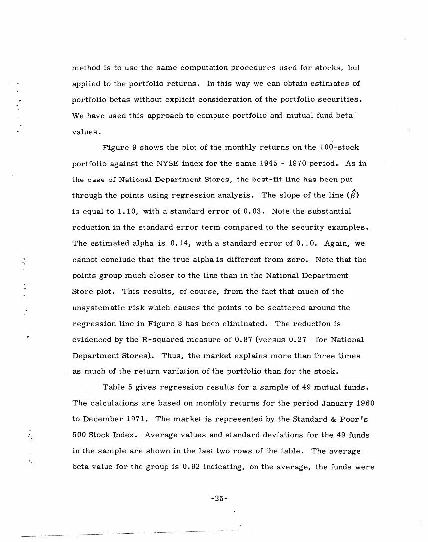
Figure 9 shows the plot of the monthly returns on the 100-stock

portfolio against the NYSE index for the same 1945 - 1970 period. As in

the case of National Department Stores, the best-fit line has been put

through the points using regression analysis. The slope of the line (j)

is equal to 1.10, with a standard error of 0. 03. Note the substantial

reduction in the standard error term compared to the security examples.

The estimated alpha is 0.14, with a standard error of 0.10. Again, we

cannot conclude that the true alpha is different from zero. Note that the

points group much closer to the line than in the National Department

Store plot. This results, of course, from the fact that much of the

unsystematic risk which causes the points to be scattered around the

regression line in Figure 8 has been eliminated. The reduction is

evidenced by the R-squared measure of 0.87 (versus 0.27 for National

Department Stores). Thus, the market explains more than three times

as much of the return variation of the portfolio than for the stock.

Table 5 gives regression results for a sample of 49 mutual funds.

The calculations are based on monthly returns for the period January 1960

to December 1971. The market is represented by the Standard & Poor's

500 Stock Index. Average values and standard deviations for the 49 funds

in the sample are shown in the last two rows of the table. The average

beta value for the group is 0.92 indicating, on the average, the funds were

-25-

less risky than the market index. Note the relatively low beta values of

the balanced and bond funds, in particular, the keystone B1, B2, and

B4 bond funds. This result is due to the low correlation between bond

and stock returns.

Up to this point we have shown that it is a relatively easy matter

to estimate beta values for stocks, portfolios, and mutual funds. Now,

if the beta values are to be useful for investment decision making, they

must be predictable. That is, beta values based on historical data

should provide considerable information about future beta values if past

measures are to be useful. The question can be asked at three levels.

How predictable are the betas estimated for stocks, portfolios of stocks,

and mutual funds? Fortunately, we have empirical evidence at each

level.

Robert A. Levy [ 13] has conducted tests of the short-run predicta-

bility (also referred to as stationarity) of beta coefficients for securities

and unmanaged portfolios of securities. Levy's results are based on

weekly returns for 500 NYSE stocks for the period December 30, 1960

through December 18, 1970 (520 weeks). Betas were developed for each

security for ten non-overlapping 52-week periods. To measure stationarity,

Levy correlated the 500 security betas from each 52-week period (the historical

historical betas) with the 52-week betas in the following period (the future

betas). Thus, nine correlation studies were performed for the ten

periods.

To compare the stationarity of security and portfolio betas, Levy

constructed portfolios of 5, 10, 25, and 50 securities and repeated the

same correlation analysis for the historical portfolio betas and future beta

-26-

_�_�__ _1_11 ��I_���___

values for the same portfolios in the subsequent period. The portfolios

were constructed by ranking security betas in each period and partitioning

the list into portfolios containing 5, 10, 25, and 50 securities. Each

portfolio contained an equal investment in each security.

The results of Levy s 52-week correlation studies are presented

in Table 5. The average values of the correlation coefficients from

the nine trials were 0.486, 0. 769, 0.853, 0. 939, and 0. 972 for port-

folios of 1, 5, 10, 25, and 50 stocks, respectively. Correspondingly,

the average percentages of the variation in future betas explained by

the historical betas are 23.6, 59. 1, 72.8, 88.2, and 94.5.

The results show the beta coefficients to be very predictable

for large portfolios, and of progressively declining predictability for

smaller portfolios and individual securities. These conclusions are

not affected by changes in market performance. Of the nine corre-

lation studies, five covered forecast periods during which the market

performance was the reverse of the preceding period (61-62, 62-63,

65-66, 66-67, and 68-69). Notably, the betas were approximately as

predictable over these five reversal periods as over the remaining15/

four intervals.

The question of the stability of mutual fund beta values is more

complicated. Even if, as seen above, the betas of large unmanaged port-

folios are very predictable, there is no a priori need for mutual fund

betas to be comparatively stable. Indeed, mutual fund portfolios are

managed, and as such, the betas may change substantially over time

by design. For example, a portfolio manager would tend to reduce the

-27-

�___I_��__�__�_____��___llsl__l___�_*_IL�il�.�--l--.--.�� ..�- --... �.---. ��-^�-�--111��111-�^��I·�_�_ l____��_n.._l����- I-

risk exposure of his fund prior to an expected market decline and raise

it prior to an expected market upswing. However, the range of possible

values for beta will tend to be restricted, at least in the longer run, by

the fund's investment objective. Thus, while we do not expect the same

standard of predictability as for large unmanaged portfolios, it is of

interest to examine the extent to which fund betas are predictable.

Pogue and Conway [ 20] have conducted preliminary tests for a

sample of 90 mutual funds. The beta values for the period January 1969

through May 1970 were correlated with values from the subsequent period

from June 1970 through October 1971. To test the sensitivity of the

results to changes in the return measurement interval, the betas for each

sub-period were measured for daily, weekly, and monthly returns. The

betas were thus based on very different numbers of observations, namely

357, 74, and 17, respectively. The resulting correlation coefficients

were 0.915, 0.895, and 0.703 for daily, weekly, and monthly betas,

respectively. Correspondingly, the average percentages of variation in

second-period betas explained by first-period values are 84, 81, and 49,

respectively. The results support the contention that historical betas

contain useful information about future values. However, the degree of

predictability depends on the extent to which measurement errors have

been eliminated from beta estimates. In the Pogue-Conway study, the

shift from monthly to daily returns reduced the average standard error

of the estimated beta values from 0. 11 to 0. 03, a 75% reduction. The

more accurate daily estimates resulted in a much higher degree of beta

predictability, the correlation between sub-period betas increasing from0.703 to 0.915.6

0.703 to 0.915.

-28-

-...... __

Figure 10 shows a plot of the Pogue-Conway first-period versus

second-period betas based on daily returns. The figure illustrates the

high degree of correlation between first- and second-period betas.

In summary, we can conclude that estimated security betas are

not highly predictable. Levy's tests indicated that an average on 24% of

the variation in second-period betas is explained by historical values.

The betas of his portfolios, however, were much more predictable, the

degree of predictability increasing with portfolio diversification. The

results of the Pogue and Conway study (among others, see footnote 16)

show that fund betas are not as stable as those for unmanaged portfolios.

On the average, two-thirds to three-quarters of the variation in fund

betas can be explained by historical values.

Further, it should be remembered that a significant portion of

the measured changes in estimated beta values may not be due to changes

in the true values, but rather the result of measurement errors. This

observation is particularly applicable to individual security betas where

the standard errors tend to be large.

-29-

· W_�_I________I____)_11___1____1

6. THE RELATIONSHIP BETWEEN

EXPECTED RETURN AND RISK

We have now developed two measures of risk and described how

they can be measured from historical data. One is a measure of total

risk (standard deviation), the other a relative index of systematic or

nondiversifiable risk (beta). We have stated our belief that the beta

measure is more relevant for the pricing of securities. Returns

expected by investors should logically be related to systematic as

opposed to total risk. Securities with higher systematic risk should have

higher expected returns.

The question of interest now is the form of the relationship

between risk and return. In this section we describe a relationship

called the "Capital Asset Pricing Model" (CAPM), which is based on

elementary logic and simple economic principles. The basic postulate

underlying the model is that assets with the same risk should have the

same expected rate of return. That is, the prices of assets in the

capital markets should adjust until equivalent risk assets have identical

expected returns. At this point, we say that the market is in an

"equilibrium" condition.

To see the implications of this postulate, consider an investor18/

who holds a portfolio with the same risk as the market portfolio (beta

equal to 1.0). What return should he expect? Logically, he should

expect the same return as that of the market portfolio.

-30-

_�___^�

Consider another investor who holds a riskless portfolio (beta

equal to zero). The investor in this case should expect to earn the rate

of return on riskless assets such as treasury bills. By taking no risk,

he earns the riskless rate of return.

Now consider the case of an investor who holds a mixture of these

two portfolios. Assume he invests a proportion X of his money in the

risky portfolio and (1 - X) in the riskless portfolio. What risk does he

bear and what return should he expect? The risk of the composite port-

folio is easily computed. Recall that the beta of a portfolio is simply a

weighted average of the component security betas, where the weights are

the portfolio proportions. Thus, the portfolio beta, Bp, is a weighted

average of the market and risk-free rate betas, that is, an average of

zero and one. Thus

p = (1 - X) 0 + X 1

= x (12)

Thus, p is equal to the fraction of his money invested in the risky

portfolio. If 100% or less of the investor 's funds are invested in the

risky portfolio, his portfolio beta will be between zero and 1. 0. If he

borrows at the risk-free rate and invests the proceeds in the risky port-

folio, his portfolio beta will be greater than 1.0.

The expected return of the composite portfolio is also a weighted

average of the expected returns on the two-component portfolios; that is,

E(Rp) = (1 - X) RF + X' E(R ) (13)

-31-

· 1 _ _ _ 1 _~~~·1 _ ~ ~ ~1_11_~ ~ ~I----.. ~ ~ ~ ^1_^.___~~.~~__ ·__. ·_____1______~~~~~_~___1·~~~~~__ ~ ~ ._ ..__~~~__1__--_-11-- -------- -

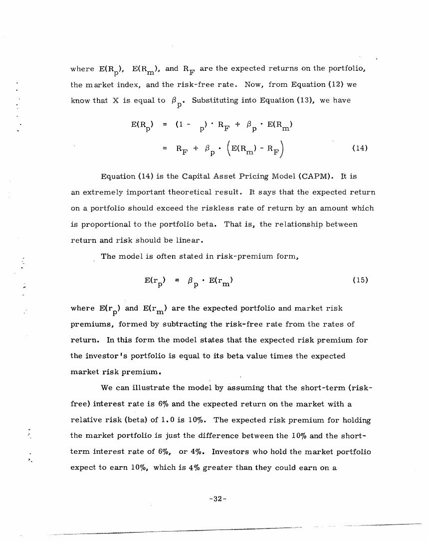
where E(Rp), E(Rm), and R F are the expected returns on the portfolio,

the market index, and the risk-free rate. Now, from Equation (12) we

know that X is equal to p. Substituting into Equation (13), we have

E(Rp) = (1- p) R F + Up E(R m )

RF + fp* (E(R m ) RF) (14)

Equation (14) is the Capital Asset Pricing Model (CAPM). It is

an extremely important theoretical result. It says that the expected return

on a portfolio should exceed the riskless rate of return by an amount which

is proportional to the portfolio beta. That is, the relationship between

return and risk should be linear.

The model is often stated in risk-premium form,

E(rp) = p E(r m ) (15)

where E(rp) and E(rm) are the expected portfolio and market risk

premiums, formed by subtracting the risk-free rate from the rates of

return. In this form the model states that the expected risk premium for

the investor I's portfolio is equal to its beta value times the expected

market risk premium.

We can illustrate the model by assuming that the short-term (risk-

free) interest rate is 6% and the expected return on the market with a

relative risk (beta) of 1.0 is 10%. The expected risk premium for holding

the market portfolio is just the difference between the 10% and the short-

term interest rate of 6%, or 4%. Investors who hold the market portfolio

expect to earn 10%, which is 4% greater than they could earn on a

-32-

_�__��_����---�� ----·---I-- "-�

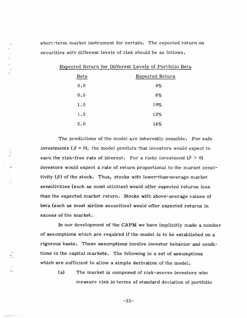
short-term market instrument for certain. The expected return on

securities with different levels of risk should be as follows.

Expected Return for Different Levels of Portfolio Beta

Beta Expected Return

0.0 6%

0.5 8%

1.0 1 0%

1.5 12%

2.0 14%

The predictions of the model are inherently sensible. For safe

investments (f = 0), the model predicts that investors would expect to

earn the risk-free rate of interest. For a risky investment ( > 0)

investors would expect a rate of return proportional to the market sensi-

tivity () of the stock. Thus, stocks with lower-than-average market

sensitivities (such as most utilities) would offer expected returns less

than the expected market return. Stocks with above-average values of

beta (such as most airline securities) would offer expected returns in

excess of the market.

In our development of the CAPM we have implicitly made a number

of assumptions which are required if the model is to be established on a

rigorous basis. These assumptions involve investor behavior and condi-

tions in the capital markets. The following is a set of assumptions

which are sufficient to allow a simple derivation of the model.

(a) The market is composed of risk-averse investors who

measure risk in terms of standard deviation of portfolio

-33-

return. This assumption provides a basis for the use of

beta-type risk measures.

(b) All investors have a common ti e horizon for investment

decision making (e.g., 1 month, 1 year, etc.). This

assumption allows us to measure investor expectations

over some common interval, thus making comparisons

meaningful.

(c) All investors are assumed to have the same expectations

about future security returns and risks. Without this

assumption, investors would disagree on expected return

and risks, resulting in a more complex situation.

(d) Capital markets are perfect in the sense that all assets are

completely divisible, there are no transactions costs or

differential taxes, and borrowing and lending rates are

equal to each other and the same for all investors. Without

these conditions, frictional barriers would exist to the

equilibrium conditions on which the model is based.

While these assumptions are sufficient to derive the model, it is not

clear that all are necessary in their current form. It may well be that

several of the assumptions can be substantially relaxed without major change

in the form of the model. A good deal of research is currently being

conducted toward this end.

While the CAPM is indeed simple and elegant, these qualities do not

in themselves make it useful in explaining observed risk-return patterns.

We now proceed to the empirical literature on attempts to verify the model.

-34-

__��1_��11�1_ � _I�___

7. TESTS OF THE CAPITAL ASSET

121PRICING MODEL

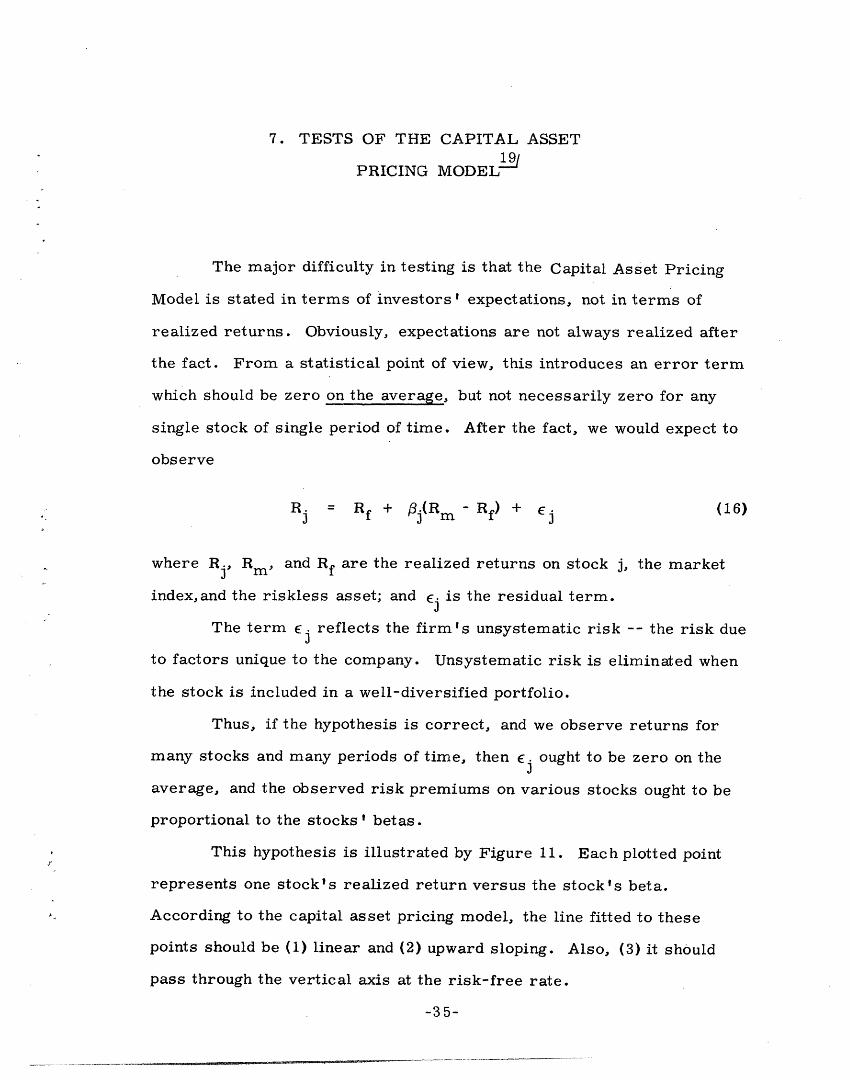
The major difficulty in testing is that the Capital Asset Pricing

Model is stated in terms of investors ' expectations, not in terms of

realized returns. Obviously, expectations are not always realized after

the fact. From a statistical point of view, this introduces an error term

which should be zero on the average, but not necessarily zero for any

single stock of single period of time. After the fact, we would expect to

observe

Rj = Rf + j(R -Rf) + Ej (16)

where Rj, Rm, and Rf are the realized returns on stock j, the market

index,and the riskless asset; and j is the residual term.

The term Ej reflects the firm's unsystematic risk -- the risk due

to factors unique to the company. Unsystematic risk is eliminated when

the stock is included in a well-diversified portfolio.

Thus, if the hypothesis is correct, and we observe returns for

many stocks and many periods of time, then Ej ought to be zero on the

average, and the observed risk premiums on various stocks ought to be

proportional to the stocks' betas.

This hypothesis is illustrated by Figure 11. Each plotted point

represents one stock's realized return versus the stock's beta.

According to the capital asset pricing model, the line fitted to these

points should be (1) linear and (2) upward sloping. Also, (3) it should

pass through the vertical axis at the risk-free rate.

-35-

_ _ ---- ----- -I I -- ~ -

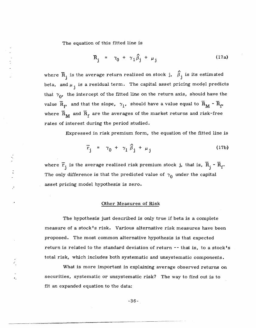
The equation of this fitted line is

j = + 77 0 j + Pi (17 a)

where Rj is the average return realized on stock j, j is its estimated

beta, and j is a residual term. The capital asset pricing model predicts

that o, the intercept of the fitted line on the return axis, should have the

value Rf, and that the slope, y 1, should have a value equal to RM - Rf*

where RM and Rf are the averages of the market returns and risk-free

rates of interest during the period studied.

Expressed in risk premium form, the equation of the fitted line is

= 70 + -1 j + pj (17b)

where rj is the average realized risk premium stock j, that is, Rj - Rf.

The only difference is that the predicted value of 70 under the capital

asset pricing model hypothesis is zero.

Other Measures of Risk

The hypothesis just described is only true if beta is a complete

measure of a stock's risk. Various alternative risk measures have been

proposed. The most common alternative hypothesis is that expected

return is related to the standard deviation of return -- that is, to a stock's

total risk, which includes both systematic and unsystematic components.

What is more important in explaining average observed returns on

securities, systematic or unsystematic risk? The way to find out is to

fit an expanded equation to the data:

-36-

--- I�_��

A A

Rj = o + 1 j + 2(SE) + j (18)

~A ~ ~ ~hAHere j is a measure of systematic risk and SE. a measure of unsystem-

20/atic risk. Of course, if the capital asset pricing model is exactly true,

then 2 will be zero -- that is, SEj will contribute nothing to the explana-

tion of observed security returns.

Empirical Tests of the Capital Asset Pricing Model

If the capital asset pricing model is right, the empirical tests

whould show the following:

1. On the average, and over long periods of time, the

securities with high systematic risk should have high

rates of return.

2. On the average, there should be a linear relationship

between systematic risk and return.

3. Unsystematic risk, as measured by SEj, should play

no significant role in explaining differences in

security returns.

These predictions have been tested in several recent statistical studies.

We will review some of the more important of these. Readers wishing

to skip the details may proceed to the summary at the end of this section.

We will begin by summarizing results from studies based on

individual securities. Then we will turn to portfolio results.

-3 7-

__ ------

Results for Tests Based on Securities

We will review two studies, one by Professor N. L. Jacob [9],

and a second by Professor M. H. Miller and M. S. Scholes [19].

The Jacob Study

This study deals with the 593 New York Stock Exchange stocks for

which there is complete data from 1946 to 1965. Regression analyses were

performed for the 1946-55 and 1956-65 periods, using both monthly and

annual security returns. The relationship of mean security returns and

beta values is shown in Table 6. The last two columns of the table give

the theoretical values for the coefficients, as predicted by the capital

asset pricing model.

The results sow a significant positive relationship between

realized return and risk during each of the 10-year periods. For example,

in 1956-65 there was a 6.7 percent per year increase in average return

for a one-unit increase in beta. Although the relationships shown in Table 6

are all positive, they are weaker than predicted by the capital asset pricing

model. In each period 1 is less than the theoretical value.

The Miller-Scholes Study

The Miller-Scholes research deals with annual returns for 631 stocks

during the 1954-63 period. The results of three of their tests are reported

in Table 7. The tests are (1) mean return versus beta, (2) mean return

^2versus unsystematic risk, (SEj) , and (3) mean return versus both beta

and unsystematic risk.

-38-

.. .. . . _ _.

The results for the first test show a significant positive relationship

between mean return and beta. A one-unit increase in beta is associated

with a 7.1 percent increase in mean return.

The results for the second test do not agree with the capital asset

pricing model' s predictions. That is, high unsystematic risk is apparently

associated with higher realized returns. However, Miller and Scholes

show that this correlation may be largely spurious (i.e., it may be due to

statistical sampling problems). For example, a substantial positive corre-

lation exists between beta and (SEj). Thus, even though unsystematic risk

may be unimportant to the pricing of securities, it will appear to be

significant in tests from which beta has been omitted. This sort of

statistical correlation need not imply a causal link between the variables.

Test number (3) includes both beta and (SEj)2 in the regression

equation. Both are found to be significantly positively related to mean

return. The inclusion of (Sj) has somewhat weakened the relationship

of return and beta, however. A one-unit increase in beta is now associated

with only a 4.2 percent increase in mean return.

The interpretation of these results is again complicated by the strongA2

positive correlation between beta and (SE.) , and by other sampling

problems. A significant portion of the correlation between mean return

and (SEj) may well be a spurious result. In any case, the results do show

that stocks with high systematic risk tend to have higher rates of return.

Results for Tests Based on Portfolio Returns

The security tests clearly show the significant positive correlation

between return and systematic risk. Tests based directly on securities,

-39-

�'-------"^----"�I----�II�----��-

however, are not the most efficient method of obtaining estimates of the

magnitude of the risk-return tradeoff. Tests based on securities are

inefficient for two reasons.

The first problem is well known to economists. It is called

"errors in variables bias" and results from the fact that beta, the

independent variable in the test, is typically measured with some error.

These errors are random in their effect -- that is, some stocks' betas

are overestimated and some are underestimated. Nevertheless, when

these estimated beta values are used in the test, the measurement errors

tend to attenuate the relationship between mean return and risk.

By carefully grouping the securities into portfolios, much of this

measurement error problem can be eliminated. The errors in individual

stocks ' betas cancel out so that the portfolio beta can be measured with

much greater precision. This in turn means that tests based on portfolio

returns will be more efficient than tests based on security returns.

The second problem relates to the obscuring effect of residual

variation. Realized security returns have a large random component,

which typically accounts for about 70 percent of the variation of return.

(This is the diversifiable or unsystematic risk of the stock.) By grouping

securities into portfolios, we can eliminate much of this "noise", and

thereby get a much clearer view of the relationship between return and

systematic risk.

It should be noted that grouping does not distort the underlying

risk-return relationship. The relationship that exists for individual

securities is exactly the same for portfolios of securities.

-40-

��_____�I� � l____·__�I___Y______1_1_1�1_1__11_��____ -

We will review the results from four studies based on portfolios --

two by Professors M. Blume and I. Friend [3] [8], a third by Professors

F. Black, M. Jensen, and M. Scholes [ 1], and a fourth by E. Fama and

J. MacBeth [6].

Blume and Friend's Study

Professors Blume and Friend have conducted two inter-related

risk-return studies. The first examines the relationship between long-run

rates of return and various risk measures. The second is a direct test of

the capital asset pricing model.

In the first study [8], the authors constructed portfolios of NYSE

common stocks at the beginning of three different holding periods. The

periods began at the ends of 1929, 1948, and 1956. All stocks for which

monthly rate-of-return data could be obtained for at least 4 years

preceding the test period were divided into 10 equal portfolios. The

securities were assigned on the basis of their betas during the preceding

4 years -- the 10 percent of securities with the lowest betas to the first

portfolio, the group with the next lowest betas to the second portfolio,

and so on.

After the start of the test periods, the securities were reassigned

annually. That is, each stock's estimated beta was recomputed at the end

of each successive year, the stocks were ranked again on the basis of

their betas, and new portfolios were formed. This procedure kept the

portfolio betas reasonably stable over time.

The performance of these portfolios is summarized in Table 8.

The table gives the arithmetic mean monthly returns and average beta

values for each of the 10 portfolios and for each test period.

___�� i�CI�II_-_-

For the 1929-69 period, the results indicate a strong positive

association between return and beta. For the 1948-69 period, while

higher beta portfolios had higher returns than portfolios with lower betas,

there was little difference in return among portfolios with betas greater

than 1.0. The 1956-69 period results do not show a clear relationship

between beta and return.

On the basis of these and other tests, the authors conclude that

NYSE stocks with above-average risk have higher returns than those with

below-average risk, but that there is little payoff for assuming additional

risk within the group of stocks with above-average betas.

In their second study [3], Blume and Friend used monthly portfolio

returns during the 1955-68 period to test the capital asset pricing model.

Their tests involved fitting the coefficients of Equation (17a) for three

sequential periods: 1955-59, 1960-64, and 1965-68. The authors also

added a factor to the regression equation to test for the linearity of the22/

risk return relationship.

Blume and Friend conclude that "the comparisons as a whole

suggest that a linear model is a tenable approximation of the empirical

relationship between return and risk for NYSE stocks over the three231

periods covered.

The values obtained for /0 and 1 are not in line with the capital

asset pricing models predictions, however. In the first two periods, 0

is substantially larger than the theoretical value. In the third period, the

reverse situation exists, with 0 substantially less than predicted. These

results imply that yl, the slope of the fitted line, is less than predicted

in the first two periods and greater in the third.

-42 -

__�___I_�__� _ ___ �__1�_____�______11�___� �1_ _____�

Black, Jensen, and Scholes

This study [1] is a careful attempt to reduce measurement errors

that would bias the regression results. For each year from 1931 to 1965,

the authors grouped all NYSE stocks into 10 portfolios. The number of

securities in each portfolio increased over the 35-year period from a low

of 58 securities per portfolio in 1931 to a high of 110 in 1965.

Month-by-month returns for the portfolios were computed from

January 1931 to December 1965. Average portfolio returns and portfolio

betas were computed for the 35-year period and for a variety of sub-

periods.

The results for the complete period are shown in Table 9. The

average monthly portfolio returns and beta values for the 10 portfolios

are plotted in Figure 12.

The results indicate that over the complete 35-year period,

average return increased by approximately 1.08 percent per month (13

percent per year) for a one-unit increase in beta. This is about three-

quarters of the amount predicted by the capital asset pricing model. As

Figure 12 shows, there appears to be little reason to question the

linearity of the relationship over the 35-year period.

Black, Jensen, and Scholes also estimated the risk-return tradeoff2 5j

for a number of subperiods. The slopes of the regression lines tend in

most periods to understate the theoretical values, but are generally of the

correct sign. Also, the subperiod relationships appear to be linear.

This paper provides substantial support for the hypothesis that

realized returns are a linear function of systematic risk values. Also, it

shows that the relationship is significantly positive over long periods of

time.

-43-

1-11�1�---1-_ 11·�1_� ---�1�����11__ _1._____���

Fama and MacBeth

Fama and MacBeth [ 6] have extended the Black-Jensen-Scholes

tests to include two additional factors. The first is an average of the

/32 for all individual securities in portfolio p, designated 2 The

second is a similar average of the residual standard deviations (SEX) forA

all stocks in portfolio p, designated SEp·. The first term tests for

nonlinearities in the risk-return relationship, the second for the impact

of residual variation.

The equation of the fitted line for the Fama-MacBeth study is

given by

- _ ^2 A 73SE Rp -T O0 +71p + 2/ 3pp SE p + fp p (19)

(19)

where, according to the CAPM, we should expect ' 2 and '3 to have zero

values .

The results of the Fama-MacBeth tests show that while estimated

values of 2 and Y3 are not equal to zero for each interval

examined, their average values tend to be insignificantly different from

zero. Fama and MacBeth also confirm the Black-Jensen-Scholes result

that the realized values of y0 are not equal to Rf, as predicted by the

capital asset pricing model.

Summary of Test Results

We will briefly summarize the major results of the empirical

tests.

-44-

-�----

1. The evidence shows a significant positive relstionship

between realized returns and systematic risk. However,

the relationship is not always as strong as predicted by

the capital asset pricing model.

2. The relationship between risk and return appears to be

linear. The studies give no evidence of significant

curvature in the risk-return relationship.

3. Tests which attempt to discriminate between the effects

of systematic and unsystematic risk do not yield

definitive results. Both kinds of risk appear to be

positively related to security returns. However, we

believe that the relationship between return and unsystematic

risk is at least partly spurious -- that is, partly reflecting

statistical problems rather than the true nature of capital

markets.

Obviously, we cannot claim that the capital asset pricing model is

absolutely right. On the other hand, the empirical tests do support the

view that beta is a useful risk measure and that investors in high beta

stocks expect correspondingly high rates of return.

-45-

______�1_____��__�1_I_

8. MEASUREMENT OF INVESTMENT PERFORMANCE

The basic concept underlying investment performance measure-

ment follows directly from the risk-return theory. The return on managed

portfolios, such as mutual funds, can be judged relative to the returns on

unmanaged portfolios at the same degree of investment risk. If the

return exceeds the standard, the portfolio manager has performed in a

superior way, and vice versa.

Given this, it remains to selectaa set of "benchmark" portfolios

against which managed portfolio performance can be evaluated. The

Capital Asset Pricing Model (CAPM) provides a convenient and familiar

set of portfolios; however, as discussed below, these are not the only

portfolios which could be used. The CAPM benchmark portfolios are

simply combinations of the riskless rate and market index. The return

standard for a managed portfolio with average beta equal to Up is equal

to the risk-free rate plus 3p times the average realized risk premium

on the market. The performance measure, ap, is equal to the difference

in the average returns between the portfolio and the standard; that is,

p p RF + p(RM - RF) (20)

where Rp, RM, and RF are the average returns for the portfolio,

market index, and riskless bond during the test period.A

Estimated values of alphs () and beta ( ) are determinedP P

as discussed in Section 5 by regressing the portfolio risk premiums on

the market risk premiums. Positive values of ap are indications of

superior performance, negative values of inferior performance.

-46-

__��I_ �� _________ls____llll_111_1_ -- �-����-�

The interpretation of the estimated alpha,, holwever, ,18nl8s ake

into consideration possible statistical measurement errors. As discussed

in Section 5, the standard error of alpha (SELL) is a measure of the extent

of the possible measurement error. The larger the standard error, the

less certain we can be that the measured alpha is a close approximation26/

to the true value.

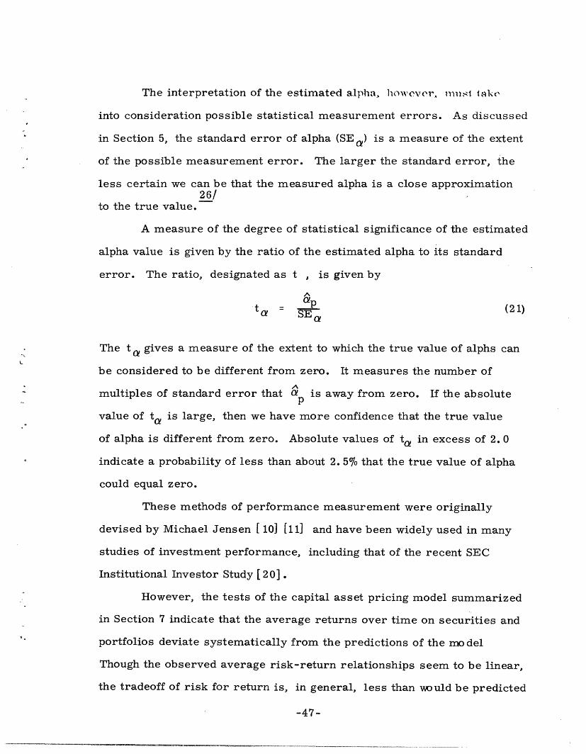
A measure of the degree of statistical significance of the estimated

alpha value is given by the ratio of the estimated alpha to its standard

error. The ratio, designated as t , is given by

oaptc = p (21)

The t gives a measure of the extent to which the true value of alphs can

be considered to be different from zero. It measures the number of

multiples of standard error that Op is away from zero. If the absolute

value of t is large, then we have more confidence that the true value

of alpha is different from zero. Absolute values of t in excess of 2. 0

indicate a probability of less than about 2. 5% that the true value of alpha

could equal zero.

These methods of performance measurement were originally

devised by Michael Jensen [ 10] [11] and have been widely used in many

studies of investment performance, including that of the recent SEC

Institutional Investor Study [ 20].

However, the tests of the capital asset pricing model summarized

in Section 7 indicate that the average returns over time on securities and

portfolios deviate systematically from the predictions of the rno del

Though the observed average risk-return relationships seem to be linear,

the tradeoff of risk for return is, in general, less than would be predicted

-47-

n r a~~~ CIQ" ~~~~~I ~~·- 1__-___ _'_____~___~__ --- _'_-------

from the CAPM. In short, the evidence suggests that the CAPM does not

provide the best benchmarks for the average return-risk tradeoffs

available in the market from naively selected portfolios.

These results do not prohibit our attempts to measure performance.

They indicate that benchmark portfolios other than those prescribed by

the CAPM would be more appropriate; but given such alternative naively

selected portfolios, the analysis could proceed in exactly the same manner

as described above. The work of Black, Jensen, and Scholes [ I ] shows

the average return from naively selected portfolios, when plotted against

risk, tends to lie along a straight line with slope somewhat less than

implied by the CAPM. These "empirical risk return" lines would seem to

be a natural alternative to the market line implied by the capital asset

pricing model. Performance would then be measured relative to the

empirical line, as opposed to the market line. A comparison of those two

standards is illustrated in Figure 13. The market line performance

measure (designated as a in Figure 13) is equal to the vertical distance

from the portfolio to the market line. The empirical line measure

(designated a 2 ) is the vertical distance from the portfolio to the empirical

line.

Since the market index ideally is composed of all assets, both

the empirical and market lines would be expected to pass through the

market index coordinates (point O in Figure 13). The intercepts on the

return axis, however, are different. The market line intercept, by

definition, is equal to the risk-free rate. The empirical line intercept

equals the average return on a portfolio with "zero beta", designated R Z .

-48-

;�,�,,II��-'^-------------·-------�-----

The existence of long-run rates of return on the cT(Io l(et:i portfolih

different from the riskless rate is a clear violation of the predictions of

the CAPM. As of this time, there is no clear theoretical understanding

as to the nature of this difference.

To summarize, empirically based performance standards would

seem to be the natural alternative to those of the capital asset pricing

model. This follows mainly because the empirical standards reflect the

actual performance of naively selected portfolios. However, the design

of appropriate empirical standards requires further research. In the

interim, the familiar market line benchmarks can provide useful informa-

tion regarding relative performance, but care must be exercised to avoid

drawing fine distinctions among portfolio results.

-49-

9. CONCLUDING REMARKS

Our task is finally completed. We have presented a brief but

hopefully comprehensive introduction to the foundations and tests of

modern portfolio theory. Our aim was to provide the reader with a first

view of the subject in hopes that his interest will be whetted for further27

study.

The major topics dealt with were the specification and measure-

ment of security and portfolio risk, the development of a hypothesis for

the relationship between expected return and risk, and the use of the

resulting model to measure the performance of institutional investors.

We have not provided a set of final answers to questions in these areas

because none currently exist. The theory and empirical evidence are in

a state of rapid evolution, and our knowledge has increased markedly in

the recent past and will surely continue to do so in the future.

-50-

__

LIST OF FIGURES

Possible Shapes for Probability Distributions

Rate of Return Distribution for Portfolio of100 Securities ..............

Rate of Return Distribution for NationalDepartment Stores ............

Standard Deviation versus Number of Issuesin Portfolio ...............

Correlation versus Number of Issuesin Portfolio ...............

Systematic and Unsystematic Risk .

The Market Model for Security Returns. ..

Returns on National Department Stores versusNYSE Index ...............

Returns on 100-Stock Portfolio versus NYSEIndex . . . . . . . . . . . .. .

Interperiod Beta Comparison: Daily Datafor 90 Mutual Funds ...........

Relationship Between Average Return (R.)and Security Risk (j) ..........

Results of Black, Jensen, and Scholes Study,1931-1965 . . . . . . . . . .

Measurement of Investment Performance:Market Line versus Empirical Standard. .

Page

52

53

.... 54

.. . . 55

.... 56

. . . 57

... 58

. . * . 59

.... 60

. . . . 61

.... 62

.... 63

. . . 64

-51-

Figure

1

2

3

4

5

6

7

8

9

10

11

12

13

X__I�II __I__�_ _I�___

. . .

Figure 1

POSSIBLE SHAPES FOR PROBABILITY DISTRIBUTIONS

1. Symmetric Probability Distribution

RE

2. Probability Distribution Skewed to Left

p 4:-

R

E

3. Probability Distribution Skewed to Right

p0a

R

E

-52-

- -·I L_ !

-~~~_

^'CII1---�---� �-_.�____I__II�---�II__.·�·�1 ..�.11_ �_ ______ --·--- _1__1·_�_�__

a---

I C.lL)

I Lt1

I.

I .

I ·I.

lLOIC.

IC-I.t

I CI.X s I ·-4 ~~~~I.¢~~~~ I ·l

10; < ~~I · NY I C

I ·I .I L'I.I ·:

I .

I CI'

I -

C·EI,.--4 I ~~~L,~]~ I~~~~~~~

Q2

* *9 * $.'4'4'

4.

..' 4' 4'4,'4* * 4 000c

-I CN (N V Co

4'4'.'.k

'

4'

$'4'4'-'*'

·

* 4·$* * $

*·$

N *k ***l tlc

K k * $ *

· * .* . $ -'4.~ .! *K $4 $

$ * - .* * *i4'$M 4 - '4 I

* '4' * .$ N* * 4' 4$4'4' $' * 4'

.* *k -' ' 4 *·4 $4 - . *

· * - . $ $ 4c

· * -* · $l * t~ * $-· N t' .k4-' ' 4'4' Ic -

$...N t *X *' .* 4*4''4 * *4'4* * * 4

* .* ,* k -4 - * 4' ,c 4' $ * $ * -* ** *M k $' * , , - *

· '* * .* $ ' , * * * * * * ' . * *l .*

tl ,k . .N -M .M ,k ~ .N .! ,K t M.4''4 O0 '4 'O,4.' M O0-) .I , O4

4' ' ' ' ' ' ''': 4.,o ~o rl 0 .'. C ,]v4.,- 4'4--I 4'".,I4'4 4"'p" L~I~l~ -tt

UL) 0 ml CU! 0 UO L L C L O C1 O Ln C L. CC. (c r ,--. O LO ! , r-I o0 L ( C, -I L(0 C) ,- .. LO C, o --I 0 ,-- 0 LAO ;1 C ) LO C (0 -I (0 r- r-. N ,. N

t ' L , 00 L n I 0 _ O N 0 C)' m .DO C I- 0 '

. . . . . . . . . . . . . . . . . . .rn 0 C) I( L 1 I I I I I I L 00 .C) ( II 'I0 L C LAO L OLC LAO LC OLC LA C L. C Lrv-I 0 0 ( 0 tb - 0 0 ( 0 I A v- C o ( C ) -> ( 0 C u- -s G( 00,I tOI rt-- L, C C c LW O-10 - , C- l-

( 0 l- I A C U r- -I 0 I I I I Ir-. r- = .I I I

,'' N1 , LtL I" CO Cr) 0 0 -'l v-I ! ,I , 1. LA I% 00 0'1 CDu -- v - v - r 4 v - v - -I - v - v -I ( N

I II II II I

I II I

I II II II II I

I II I

ilI II

I II II II I

II II II II II II II II II I

t II II II II II II II II II II II II I

I II II II II II II II II II II I

I II lI II I

I I

I I

II II II I I

1(.21Ic II LL.II I

I -- I

I (I II I* .II II II I

U)E--

C)F7O000

-40

0

~~~~~- - iH0

ofzl4H

I

0a 4 P

XO

0

O Oa) o0

04 L 11

- *4 ( 1II, ,,4 0

o= cdO -- I

11 0 * a.

a) U -

P o

h r Q

l C H

¢. Mcd

Ez0

0

E-a

_ x E

.)

_=

Cn

0

rzEplr

Pc<I:4

I -) -

I L I

a ** I

I*

I · I· IIL · I· I*

'CI * II · II · I

* I* I

0 I

I Ia * aQ) I . I

a I * I

) I ·*a *a

cs I *a

a LL

a aa Ia I

a a

.k

4'4'4'4c

4kI

4 k

. .** I* *4

C *

*.t .!4'4'·k ,,ic

4'

·* -I*

4cc * , · kk .ic· S4 -k4c'

·I *, *

9c ic .4(4'4(4'

oo o0c cO 00C c~ cO4(*4*'4(4'* 4(* 4'

* (4*'* ' * o~~~~~~~~~~~44

o: c oo o c4(4'o

CO

u-4 O C r--! r; -.

c- (. 0

C:) CO L.

r-I3 COI C4 C4

a1 atNN Cn N C

t0 Lun Lu U ULnI.0 r-t (to - CDLn o LD (. -

Co r--I r- oI

I I I I

4'.'.'*

.k-'*4k.k4k

,,k4'4'4'

*4'

*

4k.k.'4'

4'

4k

I4'4'*

k4'

4'4'4'4'

,I

,I4'4'I.'

4'4'

4'.k.k

· I· I

* ·k* ·

k .k·4'

Ic .k

·k .k4(

* I

·k .k· 4.· 4.· 4,

·*4'· 4.

·4'.9c4

oOOO

'4'4'4'4'

'

'4'4''k

CO4'4'4'4'4'(

Co

4 *

4 *

* 4

C *,'4k

4 '

o 0

4'

4o4't

4'

V -1 U) r-. L f CO Ln r T'. Cr- r r-^ _-r -- V " " r-4 r-

t-4-C)

L C

I I

PI% T-JC)!~ L I T'-

Ct cIo r Lo r-i OI In LD L rL L 00I

* . ) . . . .C N- I- rc- o U)

C14 C ' -c c- c-I a aI I I I I

rn n P_Ln LA Ln00 r oo

= rn Un

C, Ntl LrnJM t s)-r~ L) LI 00

00 C) CD

IN O OI

CT 00 00

Or-4. --

CO r O

tr-*; *~ 1'I 0

Ln

00

r-c--f

N))

Is

(-

rl

--_ Us r- G-C r-I r --I r -I -D -

I

I. aI I

I aI aI I

a II iI II aI II aa II iI II aI aI II II II Ia aI II Ia aI aa II II aI II aa II II II II aI II a

I aI II I

4' L I as to rs I I

·4 I I·OG I I

I I I I· ~ cI I

rs O oC Qooo a I I

CC N a^ a Z ox c . c" I.I I* II II I

.00CC0 I I

D oC CO I IC) (.0 L I aI CI I

I'. U C I Ir , -. c I ,, I

* * a aa aICI1sc eo a

rI c I J'-" Ii (..'

II : ILt3(.0o al U- aoo c o I I CIH -(. 3 I ~ I·- N~ a < I

oo Io I,!-r-~ I

a I

-54-

.c0

oCoO'3

co ! 0)c* ,,t -

Ia C

CoZa) Cs

C ,.0 .

r

Figure 4

STANDARD DEVIATION VERSUS

NUMBER OF ISSUES IN PORTFOLIO

STANDARDDEVIATION.-,

10 15 20 K

Source: Wagner and Lau [24], Exhibit 1.

-55-

A 4 4

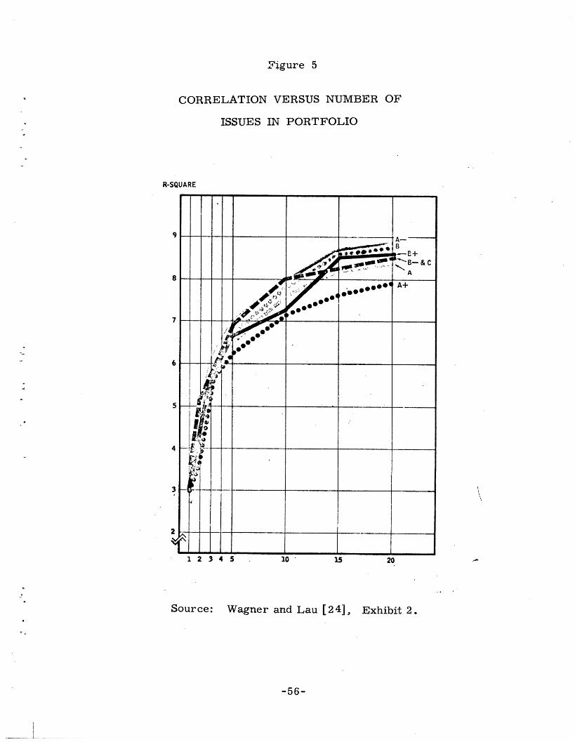
Figure 5

CORRELATION VERSUS NUMBER OF

ISSUES IN PORTFOLIO

R-SQUARE

1 2 3 4 5 10 - 15 20

Source: Wagner and Lau [24], Exhibit 2.

-56-

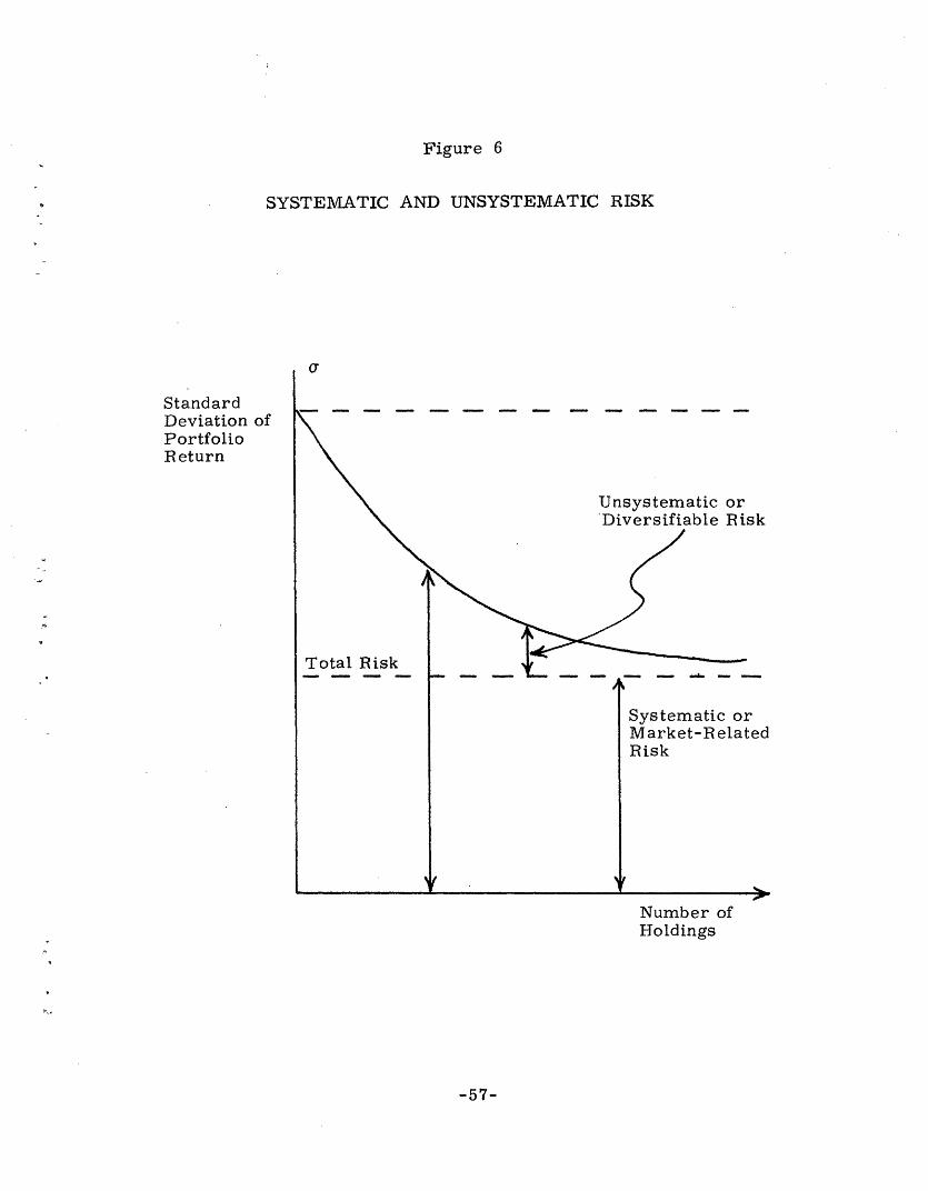
Figure 6

SYSTEMATIC AND UNSYSTEMATIC RISK

StandardDeviation ofPortfolioR eturn

Unsystematic or'Diversifiable Risk

Total Risk

Systematic orMarket-RelatedRisk

Number ofHoldings

-57-

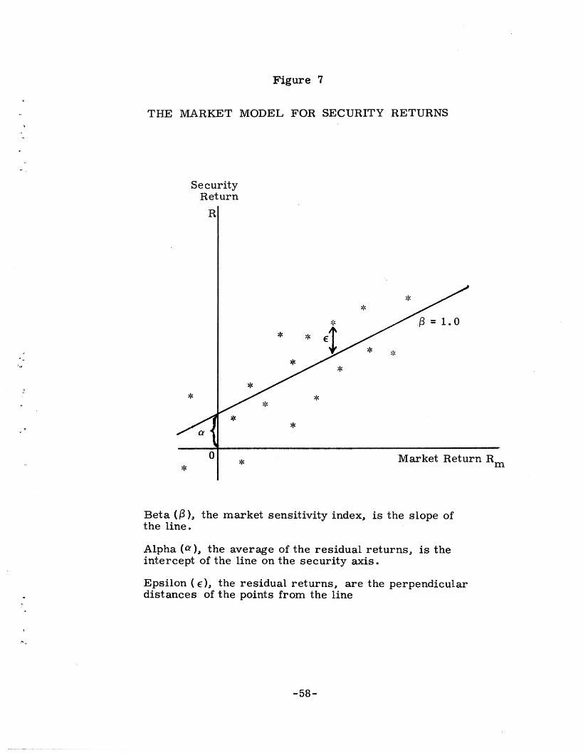
Figure 7

THE MARKET MODEL FOR SECURITY RETURNS

SecurityReturn

*

Beta (3),the line.

j. = 1.0* *

*

**

*

*

*

the market sensitivity index, is the slope of

Alpha (a), the average of the residual returns, is theintercept of the line on the security axis.

Epsilon (), the residual returns, are the perpendiculardistances of the points from the line

-58-

*

n*,

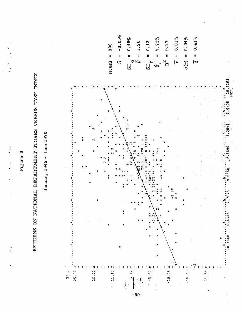
LO e- - eS e e-0 LO CD C CO t- -4 -

CO * 14 C1-4 - 0c 0 Odo 0 * * * * *CO I O ' O O o c ) o

II II II II II ii II II II II

t<(Ca WCW < P4

co

0z1 ;4

-

b

I I I >: t II I>I It I I X I I I I X I >I I I I I I I I X .1

: *'

\ * * e-4 4'

* CO co+ 44 4*

C\ CC *

I4C'44 * * * 00*( * ·I, oc o0 * *

* C; , N 4

4 ' * C C4 ' * * 4'

*~~053 * WN4' 07'

4 C t 4 1 tfr hi CO 4' N O*

4' co C O it00 ''

4' 4' * *

* r^* . GO* *s C CC

4 C Oi

C4c4 * * * 4

4'4

* *' 4'

* i C~ C 4'

* *

> I I I < I I I I > I I I I X t I I I x I I I I X I I I I I I

I?~~~~~'u-a I-.-l l_

i '- t ta

r 3 59-59-

C) cc

o Co

r-4I C-iI z

I~~~~~~~~

:,

co

U,',tr

fI

I Itx I I I I

rN,

LNc14

bD

4'4'

o

'-

0)',(DI

Cd03

9

4'4'

xw

QCa

z

VIC a

Ca fiCfHzrn

z00 E-

0a)

zH

PPw

<11

P.,w

E--q1 4:1C74

X

+I

·*

.

+

4'

4'

*'

00

'CI-E

a *

*G0

* L

'* C,*'

* u*:.0

.00* 0

* 0

* ..

:: Na

* 0·.

* I. C?

* I

* C

*

* -4* C,

.C.CI

a :

0 -

~I

00Co

C' *'

4'

*'

4'

* C

C-4COf

LIN

Co-4

I .,

4 0 -4 C) d4 t Co Vo r-4 O I o Co CO m 1 CO

0 .C O O O O O 0

It II II II 11 II II II II

(n

0zJ

it c Q 0 N

w w W 9M Vt (b

I I b

-, I I >:,,, I :,,,, > - ,,, > :, I., I i, X I,, I X g I

000

- a)~'a opq

U1 0

b13 H0

z-0HWFC

x

3-1

wrnz(/2(/2

0

a,

:

LrI

ca

Dzr

cd

'k*

49 49 49'K

49*

*K

'KC -C

.99'K

'K

49 t*. * CC* v--

N oc Nt\- : C -

c' 49 -* C*., C 't r; > tt -cl t cCi t a

; f4 .'K C 4 t' Z* t ca t -1 ,

4, rc * a C C4

* * (N Cw0 ,-

* *

* 4149494

C: c. ,1C-iC , '.

* C'K '

C :

to_

X< I I I I >: I I I I x I I I I 9 I I I I ;' I I I I X I I I I X I I I I X

L7 t > C. 0 03LC. 5= C., C) co

N . . . C

I I I 9s

_ 0 0- ' ! 1

4

* 4e

C (Nte' * C,

; C"'

k\, C.

qK

.s

to

*0 I.-

.9,

.

I .. o. No~ ~ ~ ~ ~ ~ ~ ~~ ~~ ~~~~~~~~~~~~~~~~~~~~~~~~~~~·'

'P:;~~~~~~~~~~~~~~~~~~~~~~~~~~~~~~~~~~~~~~~~~~~~~~~~~~~~~~~~~~~~'co

o~~~~~~~~~~~~~~~~~~~~~~~~~~~~~~~~~~~~~~c* 9*.

*3U.

* cN

* (N.

*0. C

* C:* C.

·cei

.o

.9

Lr?.9

* 0* C* 0

.9. I_* N

* 0

C _

'K

t,'**C4*

(N'~

*

*NJ

'K 'K

' *''K \K

+ a

.*CoC'4

'K

. C

', -t '-

I I I I

*

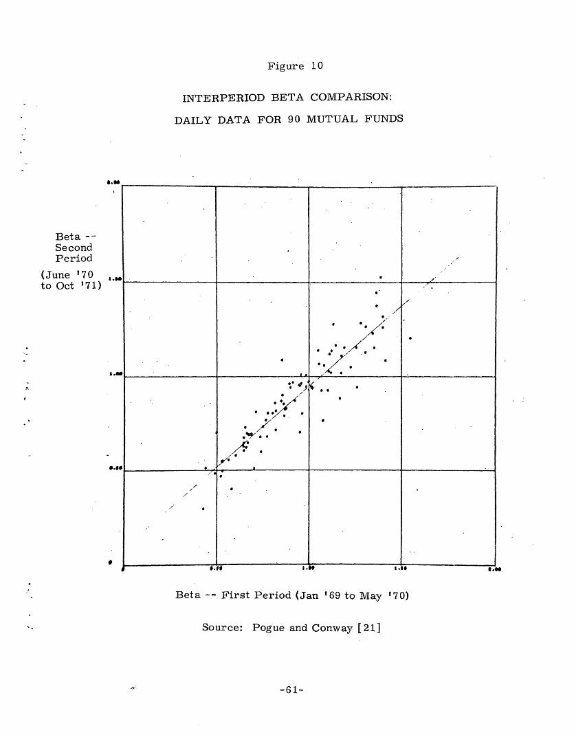
Figure 10

INTERPERIOD BETA COMPARISON:

DAILY DATA FOR 90 MUTUAL FUNDS

Beta --SecondPeriod

(June '70 ° .oto Oct '71)

S .

*.No

Beta -- First Period (Jan '69 to May '70)

Source: Pogue and Conway [21]

-61-

a

a

a

,~~~~4 r~~~~~ a

*· a

ji.~~~a .tv ..~~~~~~~

c~~~~~~~~~~

r ~ ~ ~ ~~~ r~~~~~~

r ~ ~ ~ *

a. Ht.

0

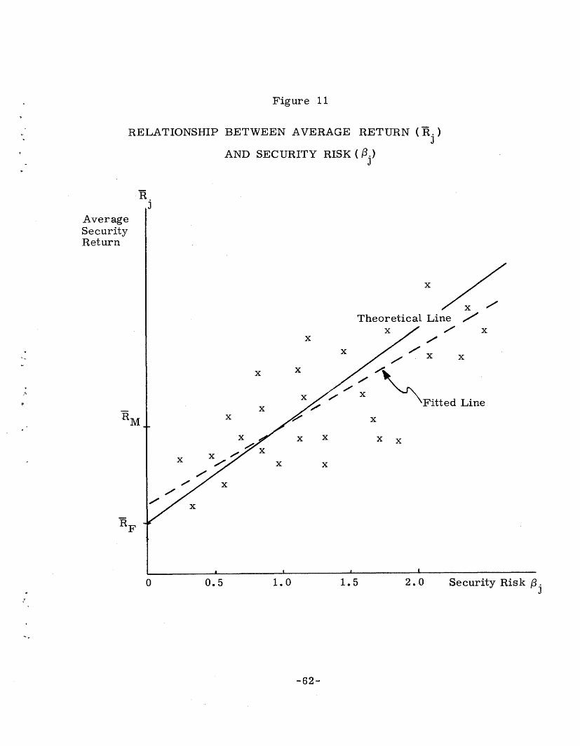
Figure 11

RELATIONSHIP BETWEEN AVERAGE

AND SECURITY

RETURN (Rj)

RISK ( j)

AverageSecurityReturn

RM

x

Theoretical Li

xx

x

x

xx

x

ne /I-/ x

x x

x

x W Fitted Linex

x x xx

x xX x

x

x

x

x

0 0.5 1.0 1.5 2.0 Security Risk 1j

-62-

I

Figure 12

RESULTS OF BLACK, JENSEN AND SCHOLES STUDY

1931 - 1965

.11-

.10

.03-

.02-

0.0 0. S 1.6SYSTEMATIC RISK

1.5 2.0

Average monthly returns versus systematicrisk for the 35-year period 1931-1965 forten portfolios and the market portfolio.

Source: Black, Jensen, and Scholes [ 1],Figure 7.

-63-

ItNTEPUPT F 0. O 19STD.EPR. El . .A:53

S.OPE = O. ia tI5TD.ERA. ER . O.Se

(,

c-

,-

I-:

_ _I_ l_ _

..C - 1 - --- 1 -.

-----·------�-�-I���

.-.I

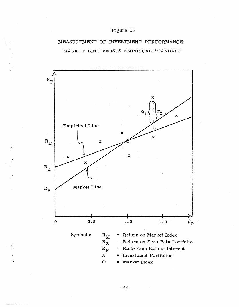
Figure 13

MEASUREMENT OF INVESTMENT PERFORMANCE:

MARKET LINE VERSUS EMPIRICAL STANDARD

0 0.5 1.0 1.5 ,p

Symbols: RM

RzRFX

O

= Return on Market Index

= Return on Zero Beta Portfolio

= Risk-Free Rate of Interest

= Investment Portfolios

= Market Index

-64-

R z

LIST OF TABLES

Table

1

Page

Risk versus Diversification for Randomly SelectedPortfolios of A+ Quality Securities . .. .. 66

Standard Deviations of 20-Stock Portfolios andPredicted Lower Limits. ............... 67

Regression Statistics for 30 Randomly SelectedSecurities . ...... . .... 68

Regression Statistics for 49 Mutual Funds. ..... . 69

Stationarity of 52-Week Betas for Portfoliosof N Securities . . . . . . . .. . . . . . . . 70

Results of Jacob's Study .... ... . . . . .. 71

Results of the Miller and Scholes Study . . . . . ... 72

Resu Its of Friend-Blume Study . . . . . . . . . . . 73

Results of Black-Jensen-Scholes Study ........ 74

-65-

Table 1

RISK VERSUS DIVERSIFICATION FOR

RANDOMLY SELECTED PORTFOLIOS

OF A+ QUALITY SECURITIES

June 1960 - May 1970

Source: Wagner and Lau [24], Table C.

-66-

Number of Average Std. Deviation Correlation with MarketSecurities in Return of Return 2Portfolio (%/month) (% /month) R R

1 0.88 7.0 0.54 0.29

2 0.69 5.0 0.63 0.40 ,

3 0.74 4.8 0.75 0.56

4 0.65 4.6 0.77 0.59

5 0.71 4.6 0.79 - 0.62

10 0.68 4.2 0.85 0.72

15 0.69 4.0 0.88 0.77

20 0.67 3.9 0.89 0.80

,

Table 2

STANDARD DEVIATIONS OF 20-STOCK PORTFOLIOS

AND PREDICTED LOWER LIMITS

(2)June 1960 - May 1970

(3)

Stock Standard Deviation Average Beta Lowerof 20-Stock Value for Limit

Qroup Portfolios Quality Group 0 * amGroup%/mo %/mo

A+ 3.94 0. 74 3.51

A 4.17 0.80 3.80

A- 4.52 0.89 4.22

B+ 4.45 0.87 4.13

B 6.27 1.24 5.89

B- & C 6.32 1.23 5.84

* am = 4.75% per month.m

Source: Wagner and Lau [24], page 6.

(4)

-67-

(1)

t

1-1 -.3 C O rn

- o o00

o C C1 ,-4 LAIIAn O O .t 00

0 0 o * 0 *

o o , C CC

0o r. iL o) C n lU ,A l_ C;.o

* 0 0 0 0 0 0 * * 0 0

o CD 0 CO 0 0 0 0 0 roooo,;,:;~:;o,:Uw wO W t 00 o -4 I0 .?r-4 "

0 C0 0 0 C l O , * * rl

00000000000

c a o c ao w.. I 0 C4

' 0 * 0

- () r-40w-I r-

(D rtn n n* 0 0 * 0

;Oo 0M r- C r4 -1~ 0 r, Loon O "ooo c r.W,-iw X ,-i - o m Ln t t b L re .ir O oo r.. o " r, w q0* * * 0 * * 0 * 0 0 * * 0 0 0 * 0 0 0 0 0 0 * *

co - C4 L o t--. Ot - r-to a00 ooD L 0 L - L ; 0 : t0 Or-4 r-4

_ - a)00co 0 _ < -4 0

C r4 03

roc1 t; oo

r P U _r, I,- o"1 0o

0000

, t. ,c Cn4C4 t N

w to to .: m C-

CO WL * - * . *- 0( a 0000 (D

tl m cl oO OO

_- 0 0 0 0 0

. m<i- r

'vd4 LI. * 0

.-I 0-I o L-

0 Lu o m- 0 0 0 0

oo - C oO Cn r (C" cn LC oo C4 0) C( ao o O

0 0 0 O 0 0 0 0 0

M-I co

C rF -W--C14 4

, 'IC O C) to

m - 0 mmI a' to -ILAto o t

in uLn tt c n)O tn

0 0 * c r o

,: ;l Co* C CO t_ W-OV V OO O -

00 LA - W w inr- O Lw . 4n 4 4n 4 N N C" r4 r* * 0 * * 0 0 * * 0

P C'400 torn n Ln

0 0 00 0 0 *

= 0 00

.. j ·0- < 0000

I I

() o

0

O

CD

Z:z

I-

rA-C.n t-

CDOO

o to oCD OOA tn m

-J

I-

C,,

U-

(4

.. Ln _:. o i.-(o t -t oD No* 0 * 0 * 0

Co C Cl Co C C

Cl LAn uD

0 0 0 C

C OO O

CO CO00 t00 Ct(N r

n ZC) C-)

<x z<

(> LU 0

C) 0 0C L.C C- J <c 0

O Z - L, X

(0

LO

I

C C0000

to to O) CO CO CDO OO

I CDOO

!I-- Z

z

- a

Z= J

0 <I-I--

F-*.00

. o Coo r- 00 c-o

* 0 0 * * 0

C) C C 0 O TC0000 -4 00

L ,I" n t -' i

UL 0 C ;000CI4 r- w- 04 tn r

LU C4(, 000 - 00,-t 4 C a , CO

O, C4 n

oo0'o oo oo ...-IC -looF-.00-! 00 Io r-l-Ir 0-I -IOCooooCoC)T- ro ) ;ooo ( C

- C4 r-I co

rn c0 * 0r-I r- v-I4 v-0I

CNO 0)0)0

to P C4 C4

00000

Ln -I ,- LI

030 000 * .* 0 0

o to o o O OC O C r; ,NON g*O*OO*O

a_ -J

o _

OCn -

--

- -- 04J > ¢ m:

c-n rH -

r-4 O c co o o o) c)

0 0 0 v-4 -4 00 C

r- m m Lr -r -t M ooI Ln . I CD LA on * 0 * * 0 * * 0 0

00000 -i 000

0 00 0 -40 O : 1_0) O tD r O -f t_ 0

c4 o4 o r- r--I -rI*~ ~ ~~~~~~~~ * J, _, ,:O~C~ IN~ ~.-' ~ -,mt H~

m0 C . wtO %Ln o-4 O 1-- r- m - MO O

U U 0 0M 0 0 0 0Ln L W (DL Ln _ALO C

00 00 O0 00

ooo) C

00 00 F .- -I 000 C-I o

00; c00 0

Lrn - t o r -t *o) 0COr- r- wLo J :oj

C 0000000000

I Ce4 c-s C totO 0f LA -t to (4

!0 0 0 0; 0 0t000000

to oC a o n r o

* * * * 0 0

000000 000Ln OC CJ

0 00 00 0 . oo G 0 00 0 0 OC "'I C O ,- I Co t -I O C' O C ,, OC O rl i l.O

I I I I

oc O

toDO (C; ,J,rn % O

O ZJ: U _

000 00000000000

to to tD tO to00 000Cl C) r )C

0O ,J0 -1

Q, O--

O- _ -

«-i 0 < U= ""="-ic.J C-)> : - I-- , O o,)

-. Iz cx c n z <

,c-- ,: oZ -Z LwI-- HJ -0O LL

- -t -wo

r I VI - v- v-I (-4

Z:z J

' 0< Li

-< -

WW cZ)--

O

v- cI ro 1-L.4 (L4I I '

* 0 0

000totoO

OC

U.

LA('4

0O0000

LD tD

totot

< I >- 0 =C

0

_ < -- *C)ZI 0 z

u z

- 3 -

C LL Z

(' C> C- F(4

000

C-)-oo

C

LLz cc- i-

C.op fMLL IWr

Wto

G O

C 00

V r-I,44O4,'-'

,O O,: r;

D C

-4o

c; ;

ttr-I lO O00

o CO

0 C

C,,--n 00

"- I--'. CO ouO 0

z

"W-

V -

c

z z

u v

-68 -

Lt C4

0 *

00 C

00 r-

,* .:

OL'-

,--

r.)WF4H

00

0C)HE-C

0rn

;in

P;-

LO

0)dq

Kt

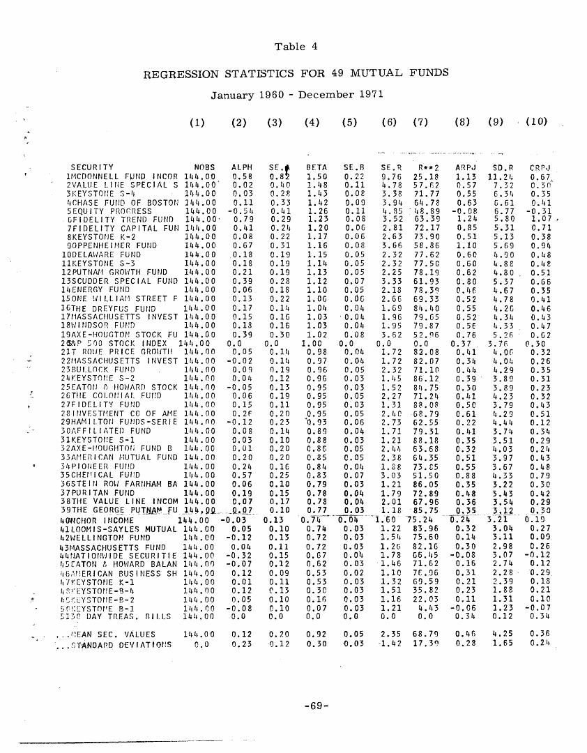
Table 4

REGRESSION STATISTICS FOR 49 MUTUAL FUNDS

January 1960 - December 1971

(2) (3) (4) (5) (6) (7) (8) (9) (10)

SECURITY1MCDONNELL FND INCOR2VALUE LINE SPECIAL S3 KEYSTO'NE S -t4CHASE FUND OF BOSTON5EQUITY PROCRESSGFIDELITY TREND FUND7FIDELITY CAPITAL FUN8KEYSTONE K-29OPPENHEIMER FUND

10DELAWARE FUND11KEYSTONE S-312PUTNAH GROCWTH FUND13SCUDDER SPECIAL FUND14ENERGY FUND15ONE WILLIA1M STREET F16THE DREYFUS FUlND17t1ASSACHUSETTS INVEST18WINDSOR FUN!D19AXE-HOUGTON STOCK FU2(:&P 500 STOCK INDEX21T ROWE PRICE GROWTH22MASSACHUSETTS INVEST23BUI LnCK FUIJID24KEYSTnONE S-225EATON & HOWARD STOCK2GTHE COLONIAL FUN!D27FIDELITY FUND28INVESTMENT CO OF AHE29HAMII TON FUJNDS-SERIE30AFFILIATEI) FUND31KEYSTONE S-132AXE-HOUGHTONl FUND B33AMERICAN fMtUTUAL FUND34 PIOIJEER FUI!D35CHE1ICAL FUND36STEIN ROW FARNHAM BA37PURITAN FUND38THE VALUE LINE INCOM39THE GEORGE PUTNAM FU49NCHOR INCOME :41 LOOMIS-SAYLES MUTUAL42WELLINGTON FUND43MASSACHUSETTS FUND44NATION!WIDE SECURITIE45 EATON & HOWARD BALAN46fiA!ERICAN BUSINESS SHi 7 EYSTONE K-14 ! 'EYSTOtNE-B-4' I Ft EYSTONE-B- 25!: EYSTOIt,!E B-I5130 DAY TREAS. BI.LLS

NOBS ALPH144.00 0.58144.00' 0.02144.00 0.03144.00 0.11144.00 -0.54144.0 0 0.79144.00 0.41144.00 0.08144.00 0.67144.00 0.18144.00 0.18144.00 0.21144.00 0.39144.00 0.06144.00 0.13144.00 0.17144 I.00 0.15144.00 0.18144.00 0.39

144;.00 0.0144.00 0.05144.00 -0.02144.00 0.09144.00 0.0;144.00 -0.05141 4.00 0.06144.00 0.15144.00 0.2F144.n00 -0.12144.00 0.08144.00 0.03144.00 0.01144.00 0.201144.00 0.24144.00 0.57144.00 0.06144.00 0.19144.00 0.0714 4 .0.Q _ Q.07144.00 -0.03144.00144.00144. 00144.00144.00144.00144.00144.00

0.05-0.120.04

-0.32-0.070.120.010.12

144.00 0.05144.00 -0.08144.00 0.0

SE .

0. 400.280.330.410.290. 24;0. 2 20.220.310.190.190.190.280.180.220.140.160.160.30

0.00. 110.140. 190.120.130.190.110.200.230.140.100.200.200.160.250.100.150.170.10

0.130.100.130.110.150.120.090.110.130.100.100.0

BETA1.501.481. 431.421.261.231.201.171.161.151.141.131.121.101.061.041.031.031.02

1.000.980.970.960.960.950.950.950.950.930.890.880.860.850.8 I0.830.790.780.780.77

0.740.740.720.720.670.620.530.530.30 0.160.070.0

SE.B SE.R R**20.22 9.76 25.180.11 4.78 57.620.08 3.38 71.770.09 3.94 64.780.11 4.85 48.890.08 3.52 63.390.06 2.81 72.170.06 2.63 73.900.08 3.66 58.860.05 2.32 77.620.05 2.32 77.500.05 2.25 78.190.07 3.33 61.930.05 2.18 78.390.06 2.66 69.330.04 1.69 84.40'0.04 1.96 79.650.01 1.95 79.870.08 3.62 52.96

0.0 0.0 0.00.04 1.72 82.080.04 1.72 82.070.05 2.32 71.100.03 1.45 86.120.03 1.52 84.750.05 2.27 71.240.03 1.31 88.080.05 2.4 0 68.790.06 2.73 62.550.04 1.71 79.310.03 1.21 88.180.05 2.44 63.680.05 2.38 64.350.04 1.88 73.850.07 3.03 51.500.03 1.21 86.050.04 1.79 72.890.04 2.01 67.960.03 1.18 85.75

0.04 .60' 75.240.03 1.220.03 1.540.03 1.260.04 1.780.03 1. 460.02 1.100.03 1.320.03 1.510.03 1.160.03 1.210.0 0.0

83.9675.6082.1666.4571.6276.9669.5935.8222.034.430.0

ARPJ SD. R1.13 11.240.57 7.320.55 C.340.63 6.61

-0.08 6.771.24 5.800.85 5.310.51 5.131.10 5.690.60 4.900.60 4.880.62 4.800.80 5.370.4;6 4.670.52 4.780.55 4.260.52 4.340.56 4.330.76 5.26

0.37 3.760.41 4.060.34 4.040.44 4.290.39 3.890.30 3.890.4/1 4.230.50 3.790.61 I4.290.22 4.440. 41 3.740.35 3.510.32 4.030.51 3.970.55 3.670.88 4.330.35 3.220.48 3.430.36 3.540.35 3.12

0.24 3.210.32 3.040.14 3.110.30 2.98

-0.08 3.070.16 2.740.31 2.280.21 2.390.23 1.880.11 1.31

-0.06 1.230.34t 0.12

,I . IEAN SEC. VALUES.,.STANDARD DEVIATIONfS

144.00 0.12 0.20 0.92 0.05 2.35 68.790.0 0.23 -0.12 0.30 0.03 -1.42 17.39

0.46 4.25 0.360.28 1.65 0.24

-69-

(1)

CRPJ0.67,0.3 0.350. 1

-0.311.07 ,0.710.380.940.480.480.510.660.350.410.460.430.470.62

0.300.320.260.350.310.230.320.430.510.120.340.290.240.430.480.790.300.420.290.30

0.190.270.090.26

-0.120.120.290.180.210.10

-0.070.34

_ � ___CIII__II__LI____a_____ll--1_ -���--

Table 5

CORRELATION OF 52-WEEK BETA FORECASTS WITH

MEASURED VALUES FOR PORTFOLIOS OF N SECURITIES

1962 - 1970

Source: Robert A. Levy [13], Table 2.

-70-

Forecast for Product Moment Correlations : N -52 WeeksEnded 1 5 10 25 50

12/28/ 62 .385 .711 .803 .933 .988

12/27/63 .492 .806 .866 .931 .963

12/25/64 .430 .715 .825 .945 .970

12/24/65 .451 .730 .809 .936 .977

12/23/66 .548 .803 .869 .952 .974

12/22/67 .474 .759 .830 .900 .940

12/20/68 .455 .732 .857 .945 .977

12/19/69 .556 .844 .922 .965 .973

12/18/70 .551 .804 .888 .943 .985

Mean dratic .486 .769 .853 .939 .972Mean

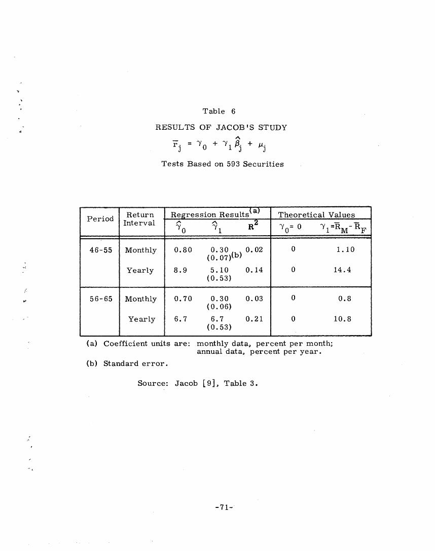
Table 6

RESULTS OF JACOB'S STUDY

rjA

= 0 + 'Yj + Pj

Tests Based on 593 Securities

Return Regression Resultsa Theoretical ValuesInterval 2 = Y

'y 0 ' 1 ' 0 1R M- R F

46-55 Monthly 0.80 0.30 0 02 0 1.10( 0 0 7 )(b)

Yearly 8.9 5.10 0.14 0 14.4(0.53)

56-65 Monthly 0.70 0.30 0.03 0 0.8(0.06)

Yearly 6.7 6.7 0.21 0 10.8(0.53)

(a) Coefficient units are: monthly data, percent per month;annual data, percent per year.

(b) Standard error.

Source: Jacob [9], Table 3.

-71-

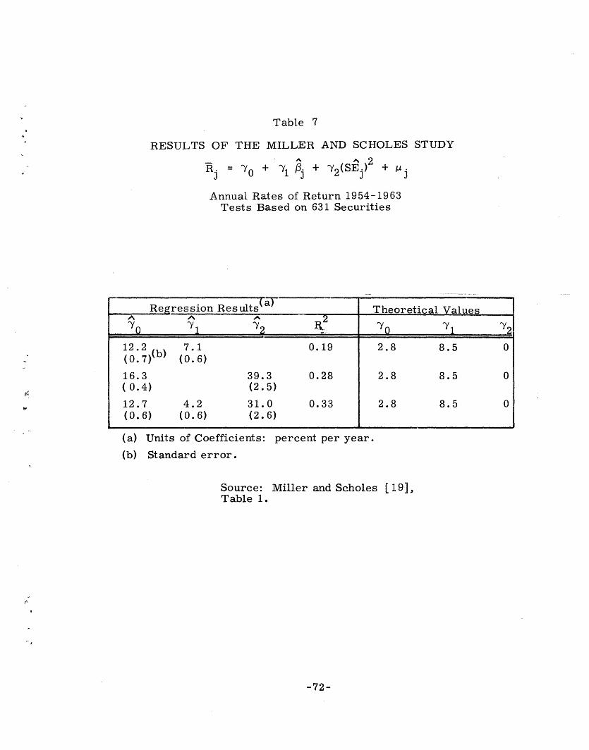
Table 7

RESULTS OF THE MILLER AND SCHOLES STUDY

Rj = 'Y + 1 j +2 (SEj) 2 + j

Annual Rates of Return 1954-1963Tests Based on 631 Securities

Regression Res ults (a ) Theoretical Values, .7 l -2

;_ )'° yY1 Y2 t o Y1 2

12.2 7.1 0.19 2.8 8.5 0( 0 . 7 ) (0.6)

16.3 39.3 0.28 2.8 8.5 0(0.4) (2.5)

12.7 4.2 31.0 0.33 2.8 8.5 0(0.6) (0.6) (2.6)

(a) Units of Coefficients: percent per year.

(b) Standard error.

Source:Table 1.

Miller and Scholes [ 19],

-72-

Table 8

RESULTS OF FRIEND-BLUME STUDY

Returns from a yearly revision policy forstocks classified by beta for various periods

Monthly arithmetic mean returns

Source: Friend and Blume [8], Table 4.

-73-

Holding Period

Port- 1929-1969 1948-1969 1956-1969

folio Mean Mean MeanNumber Return Return Return

Beta Beta Beta

1 0.19 0.79 0.45 0.99 0.28 0.95

2 0.49 1.00 0.64 1.01 0.51 0.98

3 0.67 1.10 0.76 1.25 0.66 1.12

4 0.81 1.28 0.85 1.30 0.80 1.18

5 0.92 1.26 0.94 1.35 0.91 1.17

6 1.02 1.34 1.03 1.37 1.03 1.14

7 1.15 1.42 1.12 1.32 1.16 1.10

8 1.29 1.53 1.23 1.33 1.30 1.18

9 1.49 1.55 1.36 1.39 1.48 1.15

10 2.02 1.59 1.67 1.36 1.92 1.10

,,................... _-

�� �---^--"-----~111------I-i--�

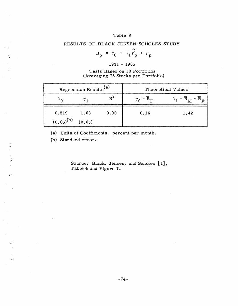
Table 9

RESULTS OF BLACK-JENSEN-SCHOLES STUDY

Rp =0 + 01p + PUp

1931 - 1965

Tests Based on 10 Portfolios(Averaging 75 Stocks per Portfolio)

Regression Results(a) Theoretical Values.Y0 R2

'0 )X1 2 /0 = RF '1 = RM - RF

0.519 1.08 0.90 0.16 1.42

(0. 0 5 )(b) (0.05)

(a) Units of Coefficients: percent per month.

(b) Standard error.

Source: Black, Jensen, and Scholes [1],Table 4 and Figure 7.

-74-

FOOTNOTES

1. Respectively Professor and Associate Professor of Finance,

Sloan School of Management, MIT. This paper was originally

prepared by us as Part I of "A Study of Investment Company

Incentive Fee Arrangements". The research was supported by

a grant from the Investment Company Institute, Washington, D.C.

2. The general expression for the arithmetic mean return for a series

of N periods is given by

- _1 RR N 2 R t

t=1

where Rt is the investment return during period t, as measured

by Equation (1).

3. The general expression for the geometric or compounded rate of

return over a series of N periods is given by

1/N= [(1 + R 1) (1 + R 2 ) ... (1 + RN)] - 1

N 1IN= [ 7 (1 +Rt)] - 1

t=1

The total return for the period is given by (1 + )N - 1.

4. The relationship between the geometric and arithmetic mean

returns is such that the arithmetic mean is always equal to or

greater than the geometric average. The difference increases

as the dispersion of the returns increases. The following

equation developed by Young and Trent [25] shows the nature

of the difference.

R= [G + a 2 (R)]1/2

-75-

I_�·_____________I�____��____��____����

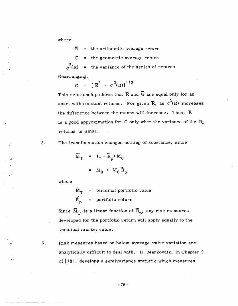
where

R = the arithmetic average return

= the geometric average return

2a (R) = the variance of the series of returns

Rearranging,

G = [/R2 - 2(R)1/2

This relationship shows that R and G are equal only for an

asset with constant returns. For given R, as (R) increases,

the difference between the means will increase. Thus, R

is a good approximation for G only when the variance of the R t

returns is small.

5. The transformation changes nothing of substance, since

M -MT = (1 + Rp) M 0

= M + M 0 Rp

where

MT = terminal portfolio value

Rp = portfolio returnp

Since MT is a linear function of Rp, any risk measures

developed for the portfolio return will apply equally to the

terminal market value.

6. Risk measures based on below-average-value variation are

analytically difficult to deal with. H. Markowitz, in Chapter 9

of [ 18], develops a semivariance statistic which measures

-76-

variability below the mean and compares it with the more

commonly used variance calculation.

7. See for example M. E. Blume [2].

8. This result follows easily for continuously compounded rates of

return. The return for N periods, Rp, is simply the sum of the

N one-period returns; that is,

Rp R 1 + R 2 + .. + R N

Now, if the one-period returns are independently and identically2

distributed with variance , then the variance of Rp will equal

No , the standard deviation fNa. The key assumption of

independence of portfolio returns over time is realistic, since

security returns appear to follow a random walk through time.

9. Two securities with perfectly correlated return patterns will

have a correlation coefficient of 1.0. Conversely, if the return

patterns are perfectly negative correlated, the correlation

coefficient will equal -1. Two securities with uncorrelated

(i.e., statistically unrelated) returns will have a correlation

coefficient of zero. The average correlation coefficient

between securities on the NYSE is approximately 0.7.

10. The reader may wish to verify that total risk (as measured by

variance) really does equal the sum of systematic and unsystematic

i-4 - risks (also measured by variance). The relationship between the

risk components is given by

-77-

2 2 2 2U =PU + E (5a)

This follows directly from Equation (5) and the assumption of

independence of Rm and E.

The R-squared term previously discussed is the ratio of systematic

to total risk (both measured in terms of variance).

,2 a2

R-squared =2

Note also that the R-squared is the square of the correlation

coefficient between security and market returns. Thus, the

correlation coefficient is equal to the ratio of 3 am to a.

11. Assuming the unsystematic returns (j) of securities to be uncorre-

lated (reasonably true in practice), the unsystematic portfolio risk

is given byN

2(p) X 2 2(Ej

j=l

2where (Ej) is the unsystematic risk for stock j. Assume the

portfolio is made up of equal investment in each security and 2 (E)

is the average value of the a (Ej). Then, Xj.= /N and

2( -2 1 2(( Up) N2 · E I (E)

(N2 ()

-78-

__�___· �_l·_·_L� _II�

which obviously approaches zero as the number of issues in the

portfolio increases.

12. That is, the risk premium for month t, rt, is given by

rt = R t - RF t

where

R t = security return in month t

RFt = risk-free ree return in month t

The conversion to risk premiums results in no substantive change

but is consistent with theoretical developments discussed in

Section 6.

13. The sample was picked to give the broadest possible range of

security beta values. This was accomplished by ranking al NYSE

securities with complete data from 1945-70 by their estimated

beta values during this period. We then selected every twenty-

fivth stock from the ordered list. The data was obtained from the

University of Chicago CRSP (Center for Research in Security

Prices) tape.

14. The commercial paper results in Table 3 are rates of return,

not risk premiums. The risk premiums would equal zero by

definition.

15. Correlation studies of this type tend to produce a conservative

picture of the degree of beta coefficient stationarity. This results

-79-

from the fact that it is not possible to correlate the true beta values

but only estimates which contain varying degrees of measurement

error. Measurement error would reduce the correlation

coefficient even though the underlying beta values were unchanged

from period to period.

16. These results are consistent with those found by N. Mains in a

later and more extensive study [ 16]. Mains correlated adjacent

calendar year betas for a sample of 99 funds for the period 1960

through 1971. The betas were based on weekly returns. The

average correlation coefficient for the 11 tests was 0. 788, with

individual values ranging from a low of 0. 614 to a high of 0. 871.

17. From this point on, "systematic risk" will be referred to simply

as risk. "Total risk" will be referred to as total risk.

18. We use the term portfolio in a general sense, including the case

where the investor holds only one security. Since portfolio return

and (systematic) risk are simply weighted averages of security

values, risk-return relationships which hold for securities must

also be true for portfolios, and vice versa.

19. The material in Section 7 was also prepared as an appendix to

testimony to be delivered before the Federal Communications

Commission by S. C. Myers and G. A. Pogue.

-80-

�_�___�1_1

A

20. SEj is an estimate of the standard error of the residual term in

Equation (16). Thus, it is the estimated value for (Ej), the

the unsystematic risk term defined in Equation (8). See column (6)

of Tables 3 and 4 for typical values for securities and mutual funds.

21. For example, skewness in the distributions of stock returns can

lead to spurious correlations between mean return and SEj. See

Miller and Scholes [19] , pp. 66, 71.

22. Their expanded test equation is

Rj 0 + + 72(j

where, according to the capital asset pricing model, the expected

value of 2 is zero.

23. Blume and Friend [3] , p. 16.

24. Table , p. 15, of Blume and Friend [3] presents period-by-period

regression results.

25- Figure 6 of Black, Jensen and Scholes [ 1] shows average monthly

returns versus systematic risk for 17 non-overlapping two-year

periods from 1932 to 1965.

26. See columns 2 and 3 of Table 4 for typical mutual fund and SEa

values.

27. There are a number of excellent references for further study of

portfolio theory. Among these we would recommend books by

Richard A. Brealey [ 4], Jack Clark Francis [ 7] , and William F.

Sharpe [23] . For a more technical survey of the theoretical and

empirical literature, see Jensen [ 12]

-81-

REFERENCES

1. Black, F., M. Jensen, and M. Scholes, "The Capital Asset

Pricing Model: Some Empirical Tests", published in Studies in

the Theory of Capital Markets, Edited by Michael Jensen.

(New York: Praeger, 1972), pp. 79, 121.

2. Blume, Marshall E., "Portfolio Theory: A Step Toward Its

Practical Application," Journal of Business, April 1970, pp. 152-173.

3. Blume, Marshall E., and Irwin Friend, "A New Look at the

Capital Asset Pricing Model", Working Paper No. 1-71, Wharton

School of Finance and Commerce, Rodney L. White Center for

Financial Research.

4. Brealey, Richard A., An Introduction to Risk and Return from

Common Stocks. (Cambridge, Mass.: MIT Press, 1969.)

5. Fama, Eugene F., "Components of Investment Performance",

The Journal of Finance, June 1972, pp. 551, 567.

6. Fama, Eugene F., and James D. MacBeth, "Risk Return and

Equilibrium: Empirical Tests", Unpublished Working Paper

No. 7237, University of Chicago, Graduate School of Business,

August 1972.

7. Francis, Jack C., Investment Analysis and Management.

(New York: McGraw-Hill, 1972.)

8. Friend, I., and M. Blume, "Risk and the Long Run Rate of

Return on NYSE Common Stocks", Working Paper No. 18-72,

Wharton School of Commerce and Finance, Rodney L. White

Center for Financial Research.

9. Jacob, N., "The Measurement of Systematic Risk for Securities

and Portfolios: Some Empirical Results", Journal of Financial and

Quantitative Analysis, VI, March 1971, pp. 815-834.

-82-

10. Jensen, Michael C., "The Performance of Mutual Funds in the

Period 1945-1964", Journal of Finance, XXIII, May 1968,

pp. 389-416.

11. Jensen, Michael C., "Risk, the Pricing of Capital Assets,

and the Evaluation of Investment Portfolios", Journal of

Business, Vol. 42, April 1969, pp. 167-247.

12. Jensen, Michael C., "Capital Markets: Theory and Evidence",

The Bell Journal of Economics and Management Science,

Autumn 1972, pp. 357-398.

13. Levy, Robert A., "On the Short Term Stationarity of Beta

Coefficients", Financial Analysts Journal, November-Decemb er1971, pp. 55-62.

14. Lintner, John, "The Valuation of Risk Assets and the Selection

of Risky Investments in Stock Portfolios and Capital Budgets",

Review of Economics and Statistics, XLVII, February 1965,

pp. 13-37.

15. Lintner, John, "Security Prices, Risk, and Maximal Gains from

Diversification", Journal of Finance, XX, December 1965,

pp. 587-616.

16. Mains, Norman E., "Are Mutual Fund Beta Coefficients

Stationary", Unpublished Working Paper, Investment Company

Institute, Washington, D.C., October 1972.

17. Markowitz, Harry M., "Portfolio Selection'', Journal of

Finance, VII, March 1952, pp. 77-91.

18. Markowitz, Harry M., Portfolio Selection: Efficient Diversification

of Investments. (New York: John Wiley and Sons, 1959.)

19. Miller, M. H., and M. S. Scholes, "Rates of Returns - in Relation

to Risk: A Reexamination of Recent Findings, " published in

Studies in the Theory of Capital Markets (see Reference 1 above),

pp. 47, 78.

-83-

_ _�___1 I � ____1�1�1_ 1��_

20. Pogue, G. A., Institutional Investor Study Report of the

Securities and Exchange Commission, Vol. 2, House Document

No. 92-64, Part 2, Chapter 4, pp. 325-347.

21. Pogue, Gerald A., and Walter Conway, "On the Stability of Mutual

Fund Beta Values", Unpublished Working Paper, MIT Sloan School

of Management, June 1972.

22. Sharpe, William F., "Capital Asset Prices: A Theory of Market

Equilibrium under Conditions of Risk", Journal of Finance, XIX,

September 1964, pp. 425-442.

23. Sharpe, William F., Portfolio Theory and Capital Markets.

(New York: McGraw-Hill, 1970.)

24. Wagner, W. H., and S. C. Lau, "The Effect of Diversification

on Risk", Financial Analysts Journal, November-December 1971,

pp. 2-7.

25. Young, William E., and Robert H. Trent, "Geometric Mean

Approximations of Individual Securities and Portfolio

Performance", Journal of Finance and Quantitative Analysis,

June 1969, pp. 179-199.

-84-

��__ II_ _�I�