an introduction to random graphs, dependence graphs, and p*
TRANSCRIPT
An Introduction to Random Graphs, Dependence Graphs, and p*
Wasserman, S. and Robins, G.
PAD 777, Xiao Liang
Definition: ERGMs
• “Exponential random graph models (ERGMs), sometimes called p* models,
- are a family of statistical models for social networks
- that permit inference about prominent patterns in the data,
- given the presence of other network structures”. (Garry Robins 2011 pp485)
Definition: ERGMs cont.
- “Each class of ERGM involves different assumptions of dependence among network ties
- Dependence is crucial and
- different assumptions of dependence are the theoretical ground for different models”
(Garry Robins 2011 pp485)
Definition: ERGMs-dependence assumption
- “The presence of some ties will encourage other ties to come into existence, to be maintained, or to be destroyed” (Garry Robins 2011 pp485).
- “The dependence assumption is thereby a theory about the basis of tie-formation processes. (Garry Robins 2011 pp485)”
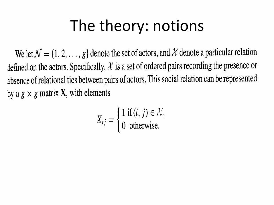
The theory: notions
The theory-dependence graph
• An observed single relational network may be regarded as a realization x=[xij] of a
• random two-way binary array X=[Xij]
The theory – dependence graph
• We specify a dependence structure for the random variables {Xij}
Since
• The entries of X cannot be assumed to be independent

The theory – dependence graph
• Thus, we introduce a dependence graph D
to help us determining the dependence structure of random variables {Xij}
The we have
D is a graph whose nodes are elements of the index set for the random variables in X
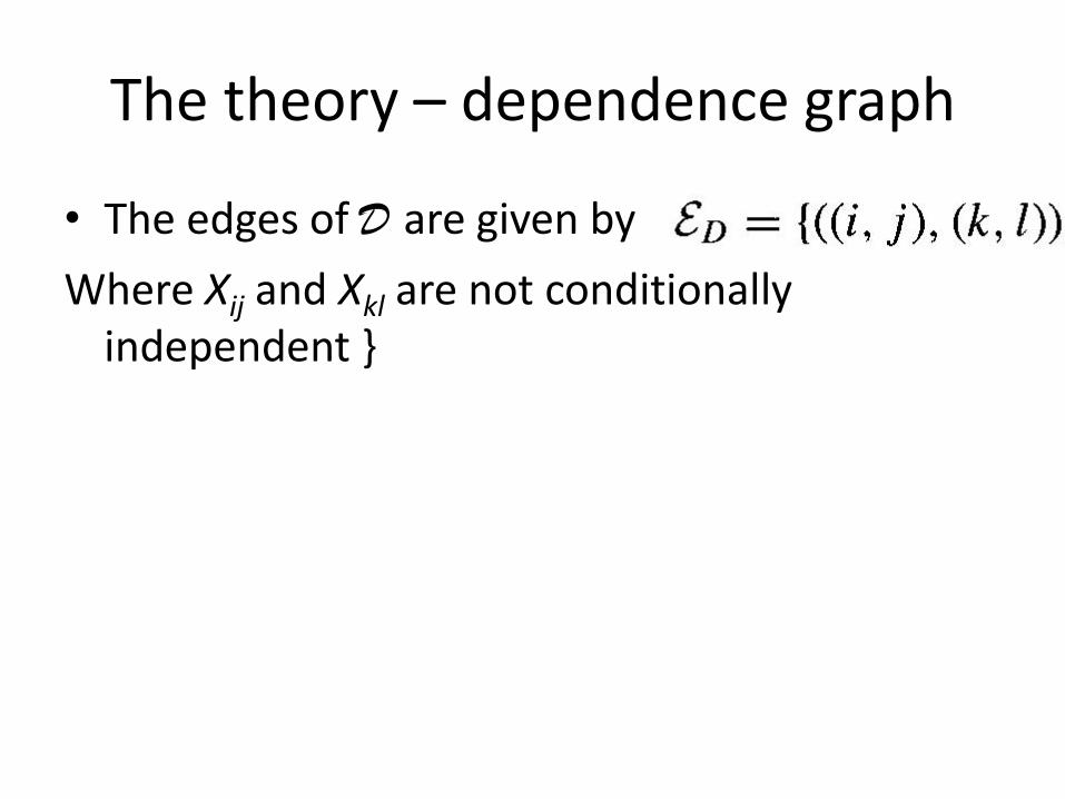
The theory – dependence graph
• The edges of D are given by
Where Xij and Xkl are not conditionally independent }
Applications –Uniform random (di)graph1 distribution
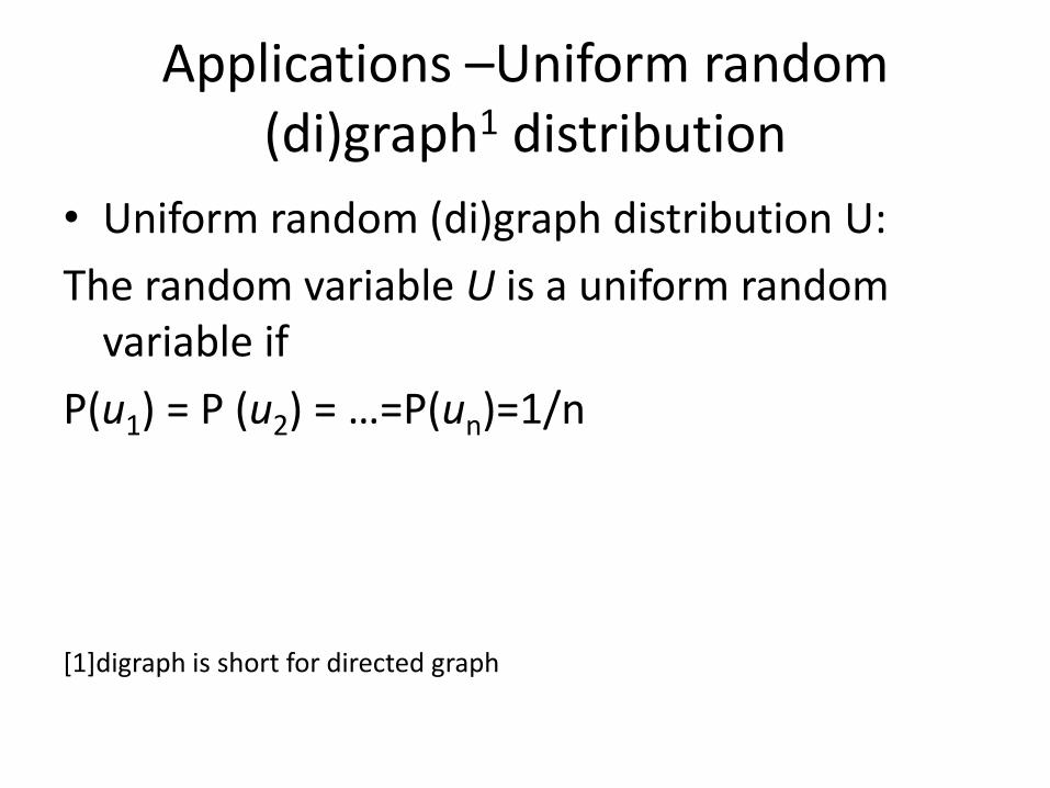
• Uniform random (di)graph distribution U:
The random variable U is a uniform random variable if
P(u1) = P (u2) = …=P(un)=1/n
[1]digraph is short for directed graph
Applications – Bernoulli Distribution Graphs
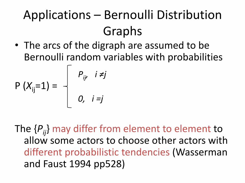
• The arcs of the digraph are assumed to be Bernoulli random variables with probabilities
P (Xij=1) =
The {Pij} may differ from element to element to allow some actors to choose other actors with different probabilistic tendencies (Wasserman and Faust 1994 pp528)
Pij, i ≠j
0, i =j
Applications – Bernoulli Distribution Graphs
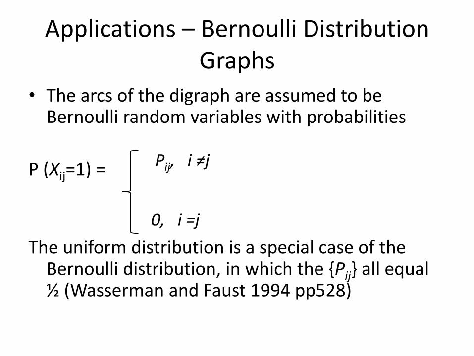
• The arcs of the digraph are assumed to be Bernoulli random variables with probabilities
P (Xij=1) =
The uniform distribution is a special case of the Bernoulli distribution, in which the {Pij} all equal ½ (Wasserman and Faust 1994 pp528)
Pij, i ≠j
0, i =j
Applications: conditional dependence U|L and U/M A N
• U|L is the uniform distribution statistically conditions on the number L of edges in the graph (pp151)
- All digraphs with L=l lines (arcs) are equally likely
• U|M A N distribution: conditions on the number M A N of dyads in the graph
(M: mutual dyads, A: asymmetric dyads, N: null dyads)
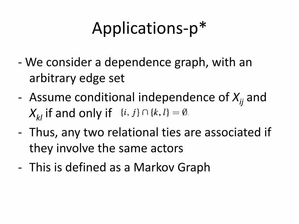
Applications-p*
- We consider a dependence graph, with an arbitrary edge set
- Assume conditional independence of Xij and Xkl if and only if
- Thus, any two relational ties are associated if they involve the same actors
- This is defined as a Markov Graph
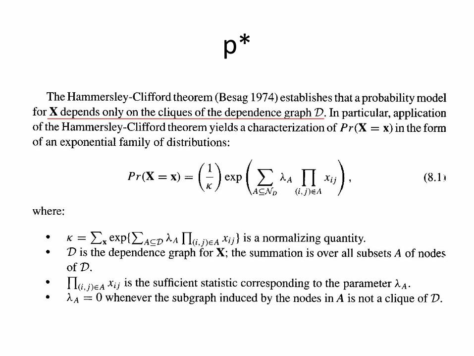
p*
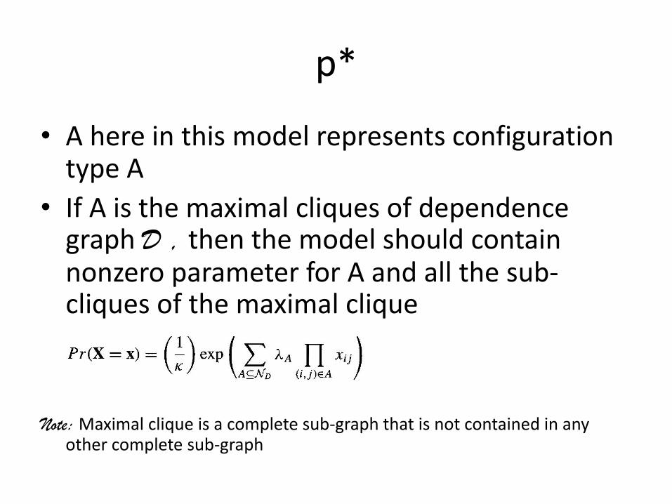
p*
• A here in this model represents configuration type A
• If A is the maximal cliques of dependence graph D , then the model should contain nonzero parameter for A and all the sub-cliques of the maximal clique
Note: Maximal clique is a complete sub-graph that is not contained in any other complete sub-graph
p*-to limit numbers of parameters
• In order to simplify the model, we do not need that overwhelmingly many parameters in the model
- Postulate a simple dependence graph D
- Make assumptions
. Usually homogeneous assumption
. in which parameters of isomorphic configurations of nodes are equated
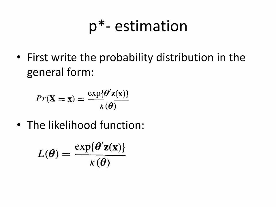
p*- estimation
• First write the probability distribution in the general form:
• The likelihood function:
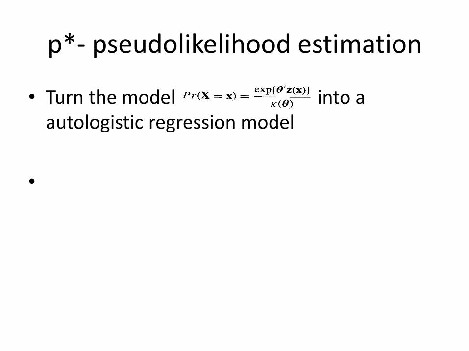
p*- pseudolikelihood estimation
• Turn the model into a autologistic regression model
•
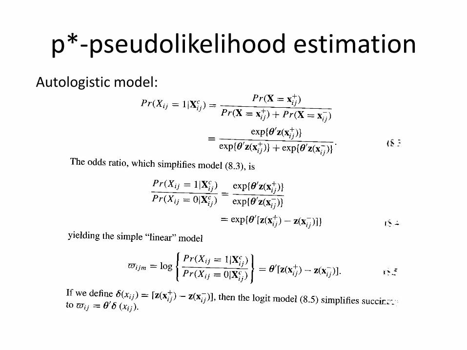
p*-pseudolikelihood estimation Autologistic model:
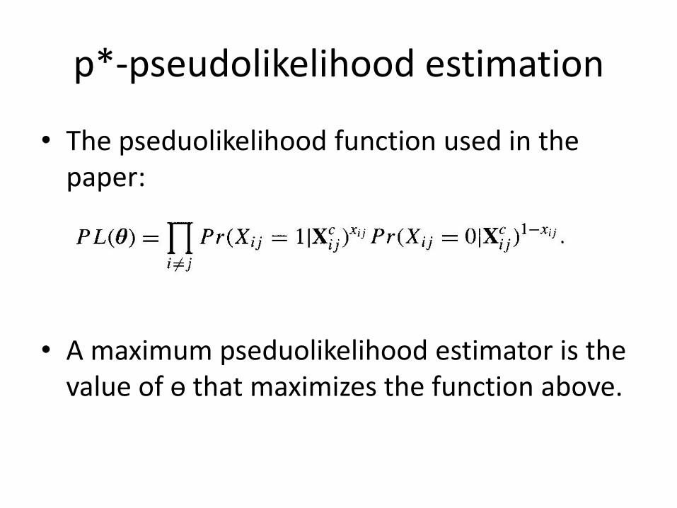
p*-pseudolikelihood estimation
• The pseduolikelihood function used in the paper:
• A maximum pseduolikelihood estimator is the value of ѳ that maximizes the function above.
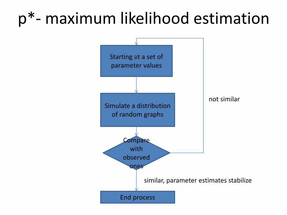
p*- maximum likelihood estimation
Starting at a set of parameter values
Simulate a distribution of random graphs
Compare
with observed
ones
not similar
End process
similar, parameter estimates stabilize
p*- maximum likelihood estimation
• Near-degeneracy
- For certain parameter values, only a handful of graphs have nonzero probability
- More often these graphs are often full or empty graphs

p*- maximum likelihood estimation
• More information of degeneracy see “Recent developments in exponential random graph
(p*) models for social networks”
Reference
• Robins, G. (2011). Exponential Radom Graph Models for social networks. In J. Scott and P. J. Carrington (eds.). The SAGE Handbook of Social Network Analysis pp484-500. Thousand Oaks, CA: SAGE.
• Wasserman, S. & Faust, K. (1994). Social Network Analysis: Methods and Applications. New York, NY: Cambridge University Press.
Recent Developments in Exponential Random Graph (p*) Models for
Social Networks
Robins et al. (2007)
PAD777 Xiao Liang
Objective of this paper
• This article reviews the new specifications for ERGM proposed by Snijders et al. (2006)
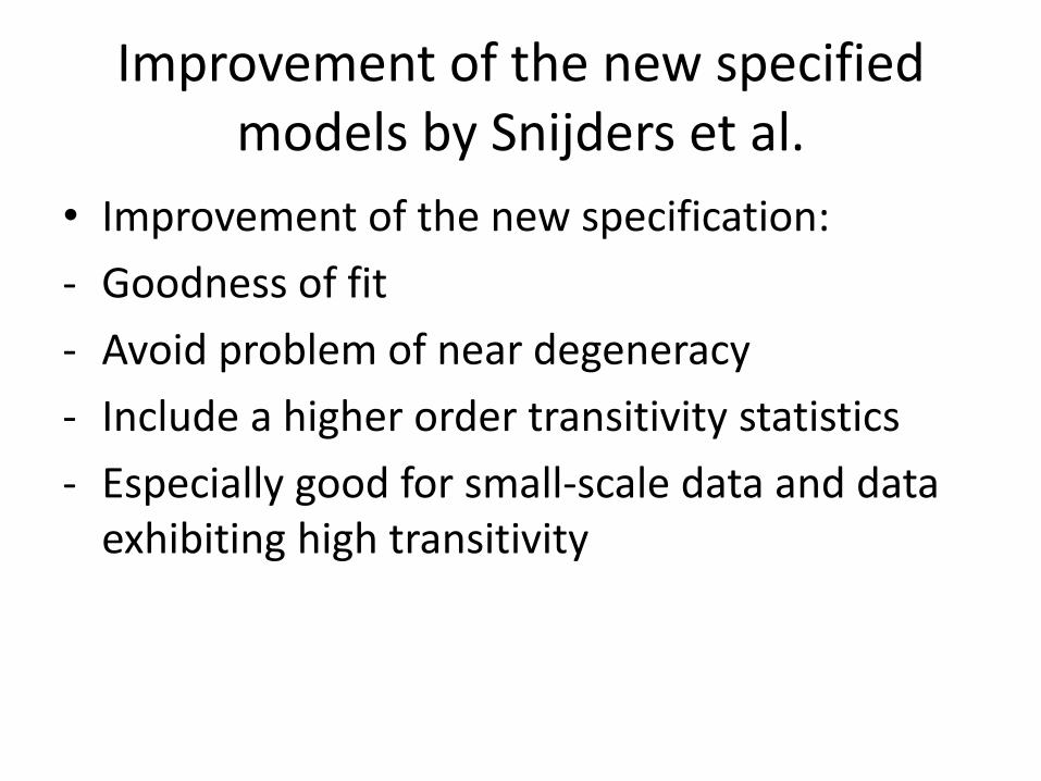
Improvement of the new specified models by Snijders et al.
• Improvement of the new specification:
- Goodness of fit
- Avoid problem of near degeneracy
- Include a higher order transitivity statistics
- Especially good for small-scale data and data exhibiting high transitivity
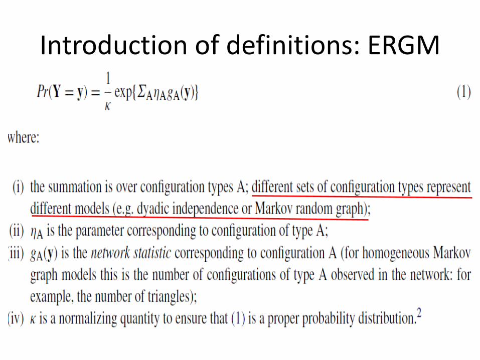
Introduction of definitions: ERGM
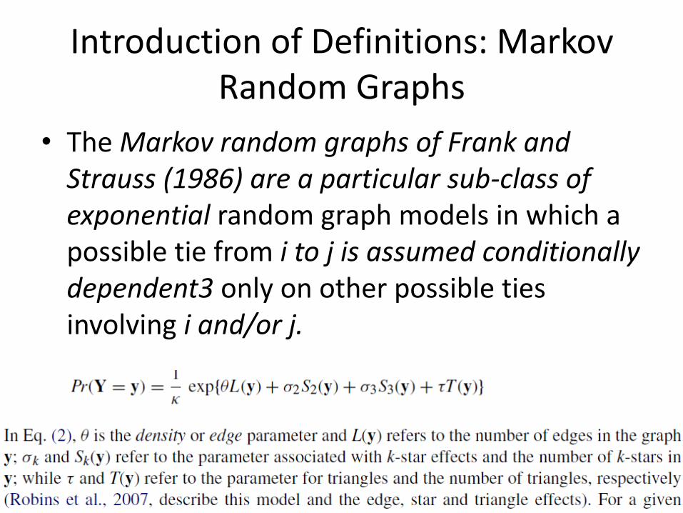
Introduction of Definitions: Markov Random Graphs
• The Markov random graphs of Frank and Strauss (1986) are a particular sub-class of exponential random graph models in which a possible tie from i to j is assumed conditionally dependent3 only on other possible ties involving i and/or j.
The Problems of old model: near degeneracy
• A graph distribution is termed near degenerate if it implies only a very few (possibly only one or two) distinct graphs with substantial non-zero probabilities (Handcock, 2003a,b)
The Problems of old model: near degeneracy
• For certain parameter values, Markov random graph distributions exhibit this (near degeneracy) property, with only nearly empty or complete graphs likely under the distribution
The Problems of old model: near degeneracy
• A softened version of near degeneracy
- a bimodal shape to the distribution:
two separate subsets of graphs, one of low density and one of density close to 1, with negligible probability for intermediate density graphs
Problems: near degeneracy
• Both version of near degeneracy are
- often observed when attempting to fit Markov models to networks where
- for instance, transitivity is in the medium to high range, as is usual for social networks
Problems: near degeneracy
• Example:
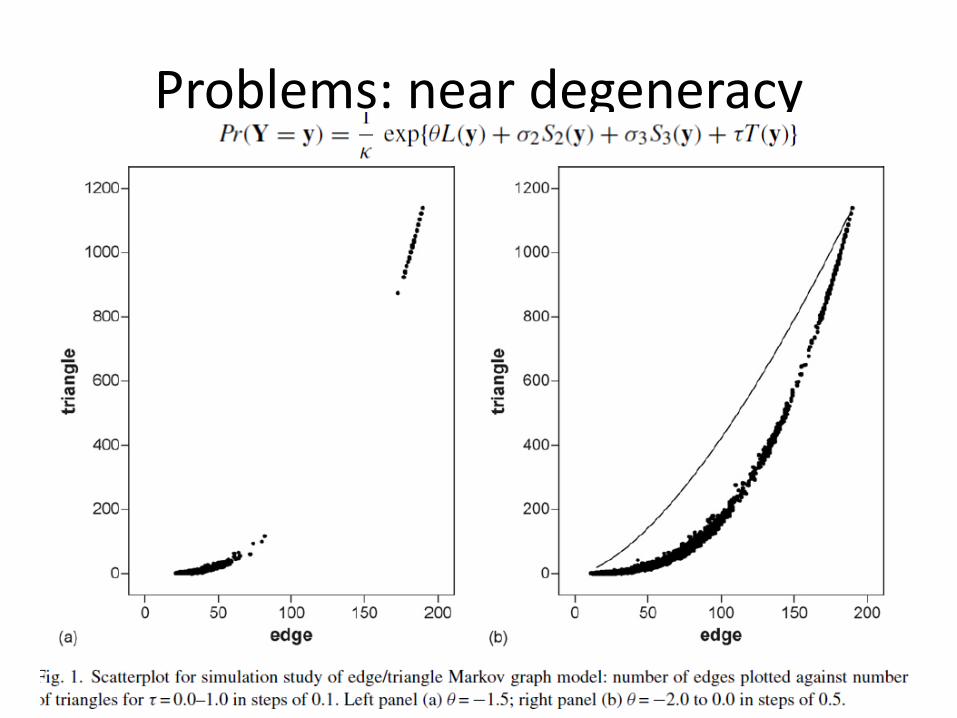
Problems: near degeneracy
• The problem of figure 1:
- Because observed social networks so frequently have triangulation much greater than Bernoulli graphs, we expect most networks of interest to lie above the lower curve (panel b)
- In other words, the simulation does not reflect the reality very well
- When we set star effects as 0, the model is inadequate for the observed network
New specifications
• Three new statistics that can be included in the model in order to avoid near degeneracy
- Alternating k-stars
- Alternating k-triangles
- Alternating independent two-paths
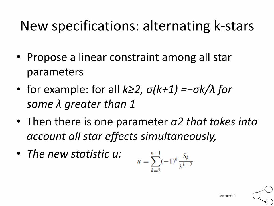
New specifications: alternating k-stars
• Propose a linear constraint among all star parameters
• for example: for all k≥2, σ(k+1) =−σk/λ for some λ greater than 1
• Then there is one parameter σ2 that takes into account all star effects simultaneously,
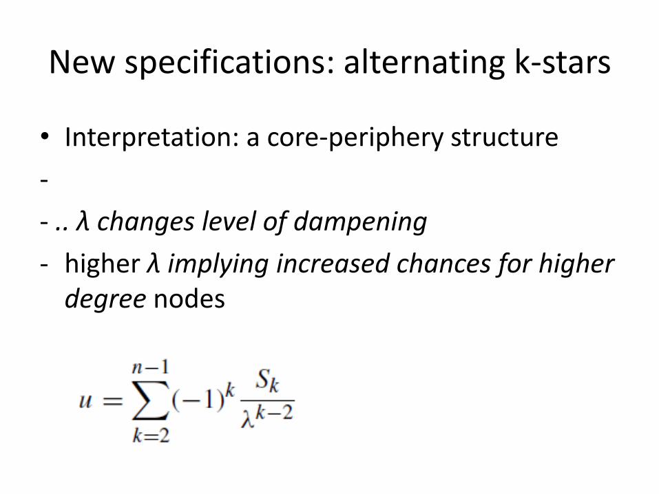
• The new statistic u:
New specifications: alternating k-stars
• for λ greater than 1, the impact of higher order stars is reduced for higher k (that is, for higher order stars) and they have alternating signs

New specifications: alternating k-stars
• Decide the value of λ
- We have used 2
- A better approach is to estimate a λ, see
Hunter, D., 2007. Curved exponential family models for social networks. Social
Networks 29, 216–230.
And see also
Hunter, D., Handcock, M., 2006. Inference in curved exponential family models for networks. Journal of Computational and Graphical Statistics 15, 565–583.
New specifications: alternating k-stars
• Interpretation:
- If the alternating k-star parameter is positive, then highly probable networks are likely to contain some higher degree nodes (“hubs”),
New specifications: alternating k-stars
• Interpretation:
- whereas a negative parameter suggests that networks with high degree nodes are improbable, so that nodes tend not to be hubs, with a smaller variance between the degrees.
New specifications: alternating k-stars
• Interpretation: a core-periphery structure
- a positive alternating k-star parameter (together with a negative density parameter) implied graphs that exhibit preference for connections between a larger number of low degree nodes and a smaller number of higher degree nodes
- akin to a core–periphery structure.
New specifications: alternating k-stars
• Interpretation: a core-periphery structure
- But once a node reaches a certain degree, the attainment of additional degrees adds little to its “popularity”.
New specifications: alternating k-stars
• Interpretation: a core-periphery structure
-
- .. λ changes level of dampening
- higher λ implying increased chances for higher degree nodes
New specifications: alternating k-stars
• Vantage of this statistic:
- Deal with some outliers – with extremely high degree nodes
- Provide a balance between positive and negative star parameters
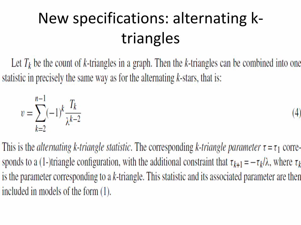
New specifications: alternating k-triangles
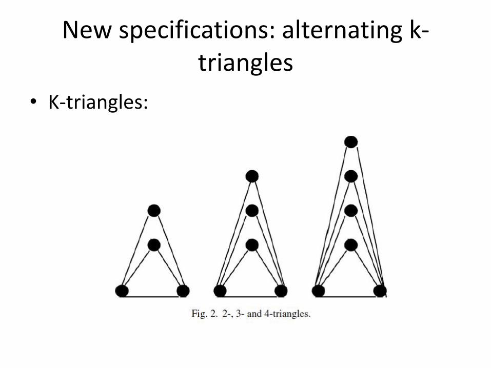
• K-triangles:
New specifications: alternating k-triangles
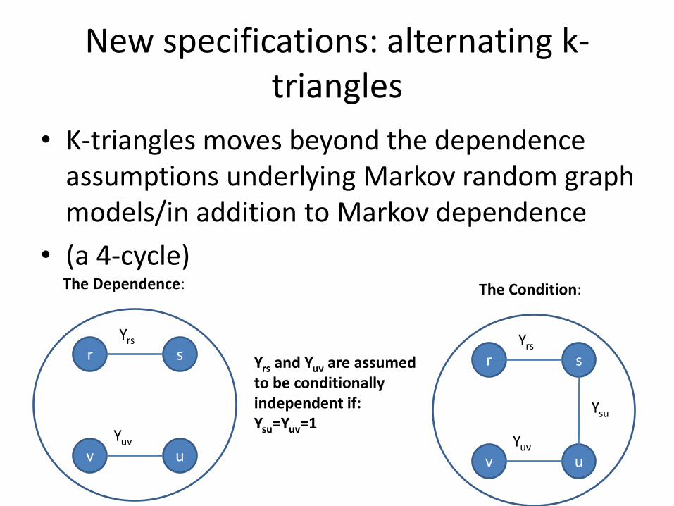
• K-triangles moves beyond the dependence assumptions underlying Markov random graph models/in addition to Markov dependence
• (a 4-cycle)
r
v u
s Yrs
Yuv
r
v u
s Yrs
Yuv
Ysu
Yrs and Yuv are assumed to be conditionally independent if: Ysu=Yuv=1
The Condition: The Dependence:
New specifications: alternating k-triangles
• k-triangles also Include Markov dependence:
- Yrs and Ysv (and so on) are also assumed to be dependent (Markov dependence)
- Hence the k-triangles configuration are more complex than simple triangles
New specifications: alternating k-triangles
• K-triangles are new higher order transitivity structures (Note: triangle is transitivity structure)
• A k-triangle is a combination of k individual triangles that all share one edge (the common base of the k triangles)
New specifications: alternating k-triangles
• K-triangles two edge variables are conditionally dependent
only if either
the Markov configuration (a common node)
or
the social circuit configuration (creation of a 4-cycle) applies
New specifications: alternating k-triangles
New specifications: alternating k-triangles
• Interpretation:
- Represent the triangulation
- A measure of the extent to which triangles themselves group together in a larger higher order “clumps”
- A positive k-triangle parameter can be interpreted as evidence for transitivity effects in the network

New specifications: alternating k-triangles
• Interpretation: the core-periphery structure
- a positive k-triangle parameter suggests elements of a core–periphery structure (dependent on other effects in the model), but in this case due to triangulation effects
- Here, a core of “core-periphery structure” is built from overlapping triangulations
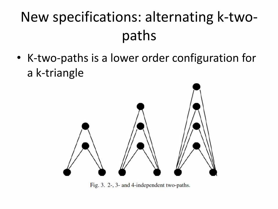
New specifications: alternating k-two-paths
• K-two-paths is a lower order configuration for a k-triangle

New specifications: alternating k-two-paths
• The motivation:
When used in conjunction with k-triangles
- K-two-paths enable researchers to
- distinguish between tendencies to
. form edges at the base of k-triangle
or
. form edges at the sides of k-triangle
New specifications: Alternative equivalent parameterizations
• The parameterizations is used to enhance interpretation and add mathematical elegance to the model
• Three types of parameterization:
- The geometrically weighted degree parameter
- The edge-wise shared partner (or ESP)
- The dyad-wise shared partner (or DSP) Reference: Hunter, D., 2007. Curved exponential family models for social
networks. Social Networks 29, 216–230.
New specifications: New specifications for directed graphs
• See
Snijders, T.A.B., Pattison, P., Robins, G.L., Handcock, M., 2006. Newspecifications for exponential random graph models. Sociological Methodology
Model Estimation
• Method: - Monte Carlo Markov chain maximum (MCMC) likelihood
estimation
• Programs for Monte Carlo maximum likelihood estimation
- SIENA
- Pnet
- Statnet is able to deal with larger data set in a relatively short time frame
Model Estimation
• Estimation statistics: (SIENA and Pnet)
- Standard errors (reliable)
- convergence t-ratio:
. how well that estimate has converged
. A small value close to zero suggests good convergent (absolute value less than or close to 0.1)
Model Estimation
• Estimation statistics (SIENA and PNet):
- t-ratio:
. If any of the t-ratios are large, this might indicate that
a. the convergence is not yet satisfactory
or
b. the model is degenerate and incapable of fitting the data
Model Estimation
• SIENA website (http://stat.gamma.rug.nl/ siena.html) and the StOCNET homepage (http://stat.gamma.rug.nl/stocnet/).
• pnet (http://www.sna.unimelb.edu.au/).
• Statnet (http://csde.washington.edu/statnet)
Models with combinations of parameters
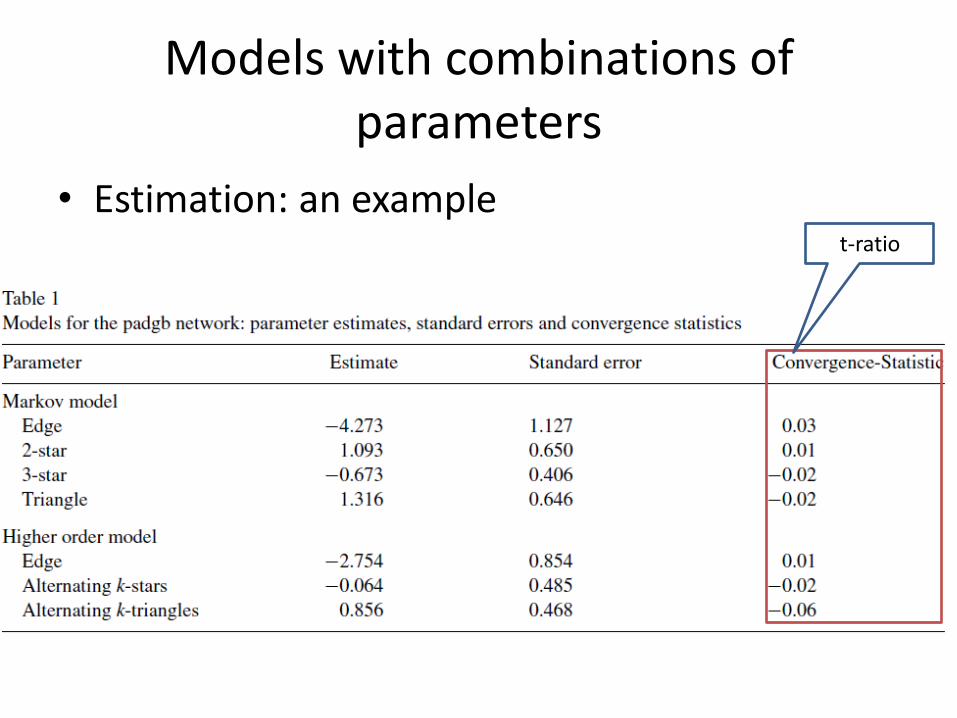
• Estimation: an example
t-ratio
Models with combinations of parameters
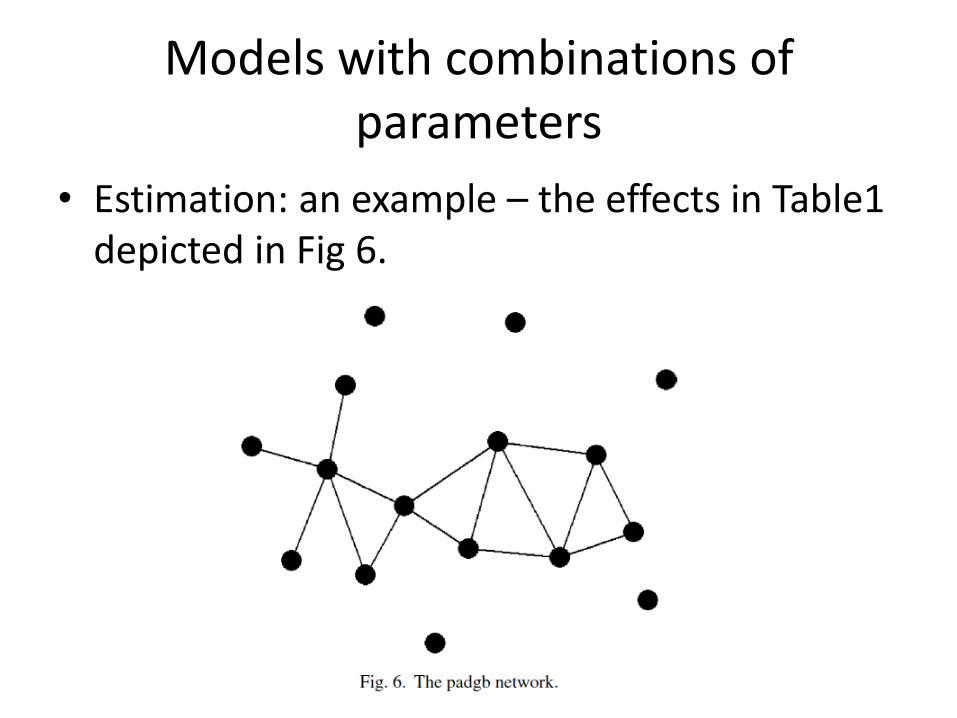
• Estimation: an example – the effects in Table1 depicted in Fig 6.
Models with combinations of parameters
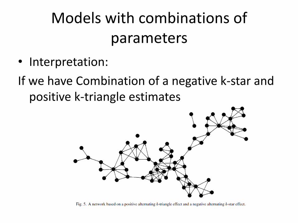
• Interpretation:
If we have Combination of a negative k-star and positive k-triangle estimates
Models with combinations of parameters
• Interpretation:
If we have Combination of a negative k-star and positive k-triangle estimates
- The network shows a triangulated core-periphery structure
- But not a degree-based core-periphery structure (hardly hubs in the network)
Models with combinations of parameters
• Interpretation:
Combination of a negative k-star and positive k-triangle estimates indicates
- So a range of models with a fixed positive k-triangle parameter, but with k-star parameters ranging from 0 to increasingly negative values, sees a move from centralization to segmentation in the network
Models with combinations of parameters
• Goodness of fit:
- to simulate the resulting distribution of graphs after the parameters have been estimated
Models with combinations of parameters
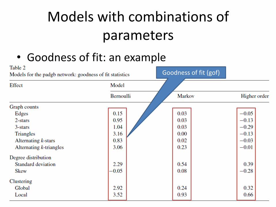
• Goodness of fit (gof statistic)
- gof statistic is the difference between the measures for the observed graph and the simulated mean, scaled by the standard deviation
- a small gof statistic indicates that the model explains this particular feature of the network well
Models with combinations of parameters
• Goodness of fit: an example Goodness of fit (gof)
Markov chain Monte Carlo estimation of exponential random graph models
Snijders, Tom A. B. (2002)
Overview
• What is this paper about?
– Discuss and propose solutions to solve problems in estimating the parameters of the p* model using Markov chain Monte Carlo (MCMC) methods
• Problems (Not useful MCMC algorithms):
– Bi- or multimodality
– Long sojourn times within regions
• Ideal (A useful MCMC algorithm):
– One region or relatively short transition times

Background
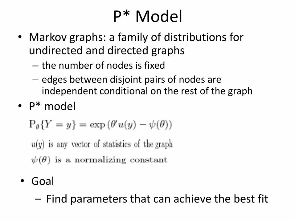
P* Model • Markov graphs: a family of distributions for
undirected and directed graphs – the number of nodes is fixed
– edges between disjoint pairs of nodes are independent conditional on the rest of the graph
• P* model
• Goal
– Find parameters that can achieve the best fit
Markov chain Monte Carlo (MCMC) Methods
• A class of algorithms for sampling from probability distributions based on constructing a Markov chain that has the desired distribution as its equilibrium distribution
• Random walk algorithms: Move around the equilibrium distribution in relatively small steps
• A good chain will have rapid mixing—the stationary distribution is reached quickly starting from an arbitrary position
•Retrieved from http://en.wikipedia.org/wiki/Markov_chain_Monte_Carlo
Markov chain Monte Carlo (MCMC) Methods used in SNA
• A simulation based method for estimating the parameters of the Markov graph distribution – Random walk algorithms:
• Gibbs sampling: Requires that all the conditional distributions of the target distribution can be sampled exactly
• Metropolis–Hastings algorithm: Generates a random walk using a proposal density and a method for rejecting proposed moves
– Compare with the equilibrium distribution • Robbins-Monro algorithm for approximating a solution to
the likelihood equation
Problems
Instability of the simulation algorithm
• Gibbs sampling procedure – For some p* models, it takes extremely long
before the Gibbs sampler seems to converge to a stable distribution
• Example 1: A directed graph with two effects – For some parameter values, the Gibbs sampler will remain
in low-density digraphs and will leave this state after some time
– For some other parameter values, the Gibbs sampler will practically permanently remain in a low-density state
– For still other values, it will practically permanently remain in a high-density state
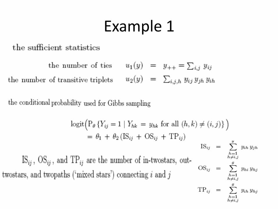
Example 1
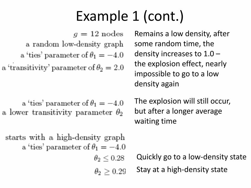
Example 1 (cont.) Remains a low density, after some random time, the density increases to 1.0 – the explosion effect, nearly impossible to go to a low density again
The explosion will still occur, but after a longer average waiting time
Quickly go to a low-density state
Stay at a high-density state
Misleading information about the expected graph statistics values
• Gibbs sampling procedure
– In some p* models, for different parameter values the Gibbs sampler switches evenly between the low-density and the high-density regime, bimodal shape. Simulation results are in practice determined by the initial state.
– Example 2: The reciprocity and twostar p* model
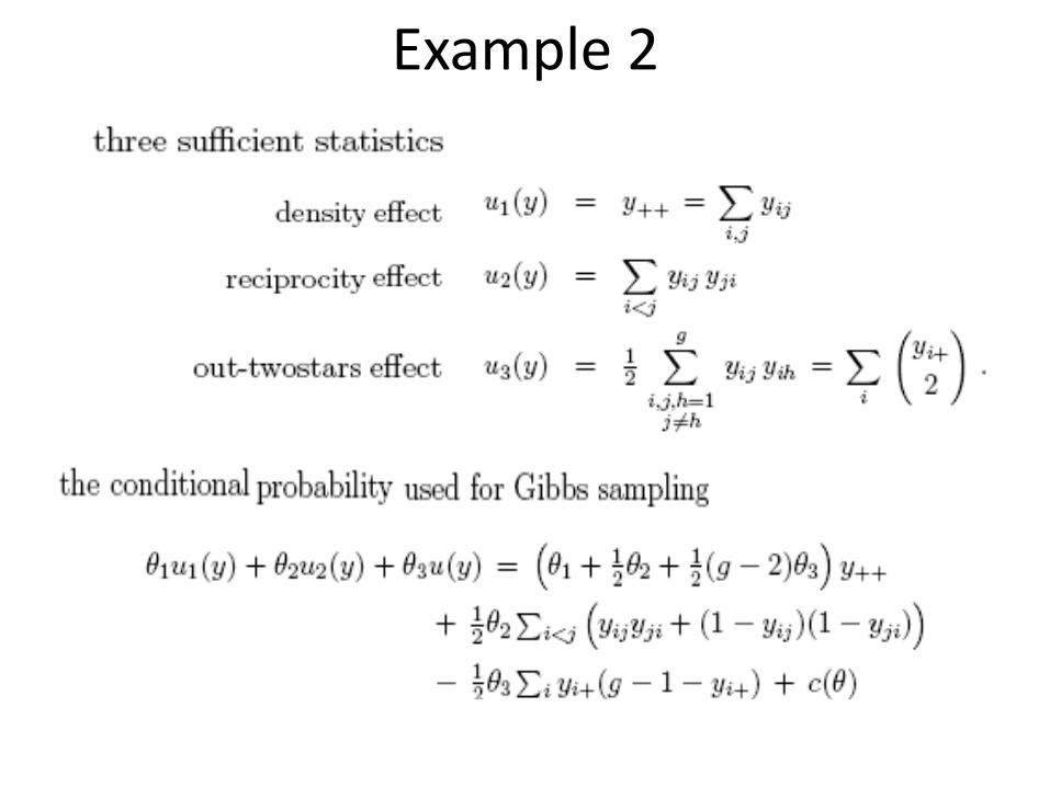
Example 2

Example 2(cont.)
Three problems
• 1) A bimodal distribution: very undesirable for modeling a single observation of a social network
• 2) A too slow convergence to the target distribution: unsuitable for generating a random draw from the distribution
• 3)Expected values of the sufficient statistics are extremely sensitive to the parameter values: cause instability of algorithms for parameter estimation
Solution
• The first problem:
– Specifying the model in such a way that the observed data set is fitted by a unimodal distribution (how? Is it possible?)
• The last two problems:
– Perhaps can be solved by an appropriate construction of algorithms
Proposals
• Augment small-step MCMC
• Algorithms by occasionally changing the graph to its complement (`inversion steps'), using probabilities that still guarantee asymptotic convergence to the desired graph distribution
Results
• For some model specifications and some data sets, this solves the convergence problems posed by bimodal distributions
• For other data sets, it fails to find an estimate that solves the moment equation to a satisfactory degree of precision
Political Connections: Assessing the
Determinants of Social Structure in Policy
Networks Hyun Hee Park
R. Karl Rethemeyer

Hyun Hee Park PhD
R. Karl Rethemeyer, PhD
Overview
This paper looks at the role of resource dependence in explaining the social structure of policy networks while controlling for the effects of microstructure.
This analysis utilizes ERGM techniques to control for the effects of network substructures like reciprocity and transitivity
Resource Dependency Theory
This analysis will demonstrate that decreased resource availability can cause network segmentation that can change the composition and nature of the relationships among network members.
Examines the balancing operations undertaken by resource holders and seekers.

Background
Policy Networks: An arena where policy deliberation and policy making occur outside the recognized parameters of public administration
Examples? “ Three Men in a Room?”
Resource Dependency Theory
A theoretical framework to understand policy networks (Hatmaker and Rethemeyer 2008, Rethemeyer 2007, 2007) This framework focuses on the necessity of resource seeking/gathering as the bonding factor that holds policy networks together. Proposes that hierarchal elements of networks and coalition formation result from attempts to mitigate dependence.

Analysis Questions
What role does resource dependence play in explaining the relational structure of a policy network and the behavior of public and private organizations in terms of their relative choice in it?
What does this tell us about network management, a task public managers increasingly undertake?

Part I. Policy Network Framework
Underlying questions are:
How is policy made?
How does the public think policy is made?

Policy Networks
Policy networks are the products of networks that span the public and private sector. Actors include: public agencies, legislative offices, interest groups, corporations, and non-profits that have a stake in public decisions within a certain policy area.
The decisions in question effect all members of a network and their ability to function

Policy Networks Cont’d
Why do organizations participate in policy networks?

Two Kinds of Resources
Material Institutional Resources (MIRs): a set of financial, political, human, informational, and institutional resources that are leveraged to support preferred policy objectives.
Social Structural Resources (SSRs): resources that arise from patterns of interaction between three or more social actors in a network. This assumes that patterns of communication and resource transfer are not random.

MIRs and SSRs
In equilibrium, MIRs and SSRs reinforce one another.
Emerson, 1962 suggested that SSRs can be accumulated in four ways.

Accumulating SSRs
Power Network Extension---seeking new sources of resource suply
Withdrawal---seeking to reduce the need for scarce resources
Coalition Formation---seeking to work with others in coalitions
Emergence of Status---seeking to collectively grant status by elevating a dominant player

Why is all of this important?
Relations in policy networks are not a mirror reflection of dependence
This is evinced by the lack of hub and spoke arrangements
So how can we examine resource dependence and the generic social pressures that impact network functioning?
Beyond Resource Dependence
Local interactions and microprocesses impact the global network structure (Johnson, 1986; Pattison and Robbins 2002)
Triadic closure: Focal actors stance is affirmed and reinforced by two other actors who agree with the focal actor and each other
Reciprocity

ERGM: A New Tool
So Resource Dependence Theory may not explain all the connections and factor in policy network functioning.
ERGMs offer a unique way to study these generic social pressures and their impact on policy networks

Research Questions
What role does resource dependence play in fostering connections? How does that role play out in different resource environments?
What factors help to promote or discourage connections between policy network members?

Research Questions
What role do broad network properties and substructures play in explaining connections in policy networks?
How do participants on a policy network manage dependencies in a resource scarce environment?
What do our findings suggest regarding the relational environment of public management?

Case Study and Research Methods
Two waves of data collected in 1998 and 2005
Information was collected for two measures of potential power on the nature of financial flows and regulation.
The model uses network variables such as reciprocity preference for higher out degree nodes, preference for higher in degree nodes, alternating k-triangles, etc.

Methods
Other basic organizational data was also gathered and used to construct variables for total budget, geographic proximity to the capital city, sector membership, and type of organization.
Measuring Influence
This study examines the direction of resource and information flows.
Three attribute related parameters for each dependence variable are included in the model: ego, alter and same.
Attribute Values
A positive value for an attribute ego paramter suggests that actors with higher values on the attribute in question make more ties (higher out degree
A positive value for an attribute alter paramter are likely to receive more ties (higher in-degree)
A positive value for an attribute same is indicative of actors preferring similar attributes (homophily)

ERGM Brief Review
After parameters are generated, t-rations for each are calculated to assess the degree of fit ◦ A good model has little or no divergence from the actual data. This means we are looking for t-ratios that are as close to zero as possible. Tables 2 and 3 have t-rations of less than .1
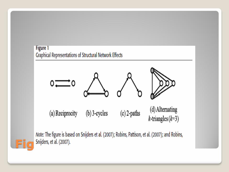
Figure 1
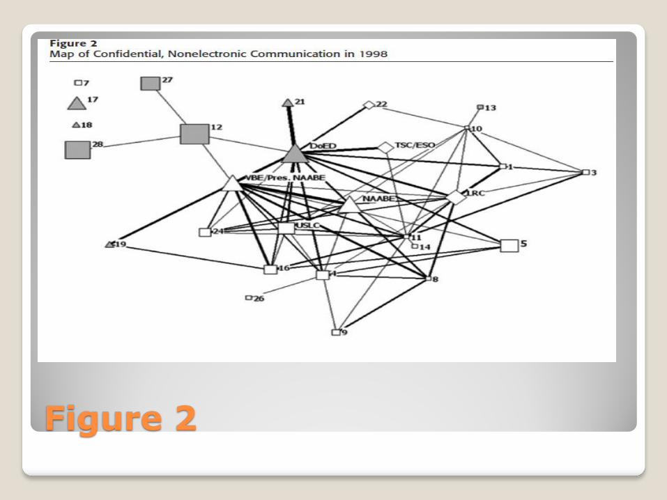
Figure 2
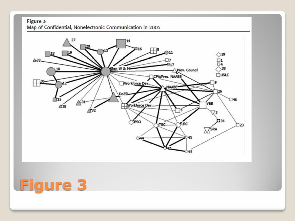
Figure 3
Goodness of fit is examined using SIENA. Tables 2 and 3 were significant at 1% level which indicates that the models fit these particular policy networks very well
Each parameter is assessed as to whether or not the variable has explanatory power in the model. A series of goodness of fit tests with one degree of freedom are run for each parameter. The threshold of significance is the standard 5% or 10% levels. Variables are then repeatedly added or removed in the model selection process
This process demonstrates that some effects are so prevalent of strong that they could not have been generated randomly or by chance in this policy network.

Longitudinal Data Adult Basic Education Findings
Recall that the ABE network data was collected before and after a dramatic change in environment
Four Complementary Explanations
The ABE network was impacted by dramatic budget cuts that would have effectively stopped provider operations
As a result the industry association coordinated a response
The network changed under the influence of this massive resource crisis.
A group of technical assistance organizations became major player in the network between data collections
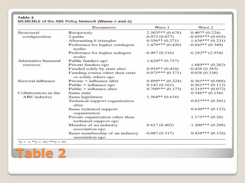
Table 2
Table 2
Table 2 reports the final models that resulted from this analysis. It is a reduced set of variables with a significant coefficients in at least one model
This suggests a shift from a core periphery structure base don reciprocity to a segmented structure base don transitive closure

Table 3

Table 3
Table 3 shows that financial resources were influential in shaping communications patterns. The distinction between the first and second wave show a dearth of private funding in wave one, and a significant presence in wave 2.
What else does table 3 show?

Table 3
Reports confidential communications that occur between network members 2-3 times a month or more. Thicker lines indicate higher levels of communication. A similar pattern existed in the first wave data as well/
Three Findings
Competition facilitates local concentration but runs contrary to centralization.
Getting in to a network is more difficult when available resources decrease
Trust is a big issue

Resources in a Crisis
Actor efforts to secure resources fall into two types of actions:
1.) Finding alternative sources of MIRs directly (private sector), 0r
2.) Using SSRs to get MIRs from the state (effective lobbying)
Propositions about Policy Network Structure and Evolution
1.) Change in dependence configurations change network structures
1a.)Dependence coupled with power imbalances causes network segmentation, particularly sectoral and sub sectoral relational polarization
2.) Influence and sector are not independent drivers of relational structure but interat with one another

Propositions
3.) Crisis sweeps away the weaker less connected players
4.) Broad social pressures, such as reciprocity and transitivity affect inter-organizational resource dependence.
5.) Material resources affect relational structure but more through resource seeking and preservation strategies than direct transfer potential