Modeling high-dimensional dependence with directedacyclic graphs

Maochao Xu

Department of MathematicsIllinois State University

mxu2@ilstu.edu

Directed acyclic graph

A directed acyclic graph (DAG), is a directed graph with no directed cycles. It has beenwidely used in many areas such as computer science, engineering, medical diagnosis,and crime risk factors analysis etc.

Example: Medical diagnosis

Example: Car insurance

Directed acyclic graphLet us consider n random variables X1, . . . ,Xn, a directed acyclic graph with nnumbered nodes, and suppose node j (1 ≤ j ≤ n) of the graph is associated to the Xjvariable. Then the graph is a Bayesian network, representing the variables X1, . . . ,Xn,if:

P(X1, . . . ,Xn) =n∏

j=1

P(Xj | parents(Xj )

),

or

f (x1, . . . , xn) =n∏

j=1

f(xj | parents(xj )

),

where parents(Xj ) denotes the set of all variables Xi , such that there is an arc fromnode i to node j in the graph.Example:

f (x1, x2, x3, x4) = f1(x1)f2|1(x2|x1)f3|1(x3|x1)f4|23(x4|x2, x3).

Any joint probability distribution may be represented by a Bayesian network.

Multivariate distribution

Multivariate real-valued distributions are of paramount importance in a variety of fieldsranging from computational biology and neuro-science to economics to climatology.Choosing and estimating a useful form for the marginal distribution of each variable inthe domain is often a straightforward task. In contrast, aside from the normalrepresentation, few univariate distributions have a convenient multivariategeneralization. Indeed, modeling and estimation of flexible (skewed, multi-modal,heavy tailed) high-dimensional distributions is still a formidable challenge.

In the literature, standard references on the theory of graphical models are mainlylimited to the assumption of joint normality as far as continuous variables areconcerned. At the same time, it is well known from the literature on statistical modelsfor financial markets that the assumption of joint normality may lead to severeunderestimation of certain risks and, in a more general sense, fails to yield suitablemodels in many applications, see, for instance, McNeil et al. (2005).

How to model high dimensional non-normal (or non-Gaussian) dependence?

Copula

Assume that (X1, . . . ,Xn) is a set of real-valued continuous random variables. Then,the joint distribution function is

F (x1, . . . , xn) = P(X1 ≤ x1, . . . ,Xn ≤ xn).

Then, by Sklar Theorem, there exist a unique Copula function C such that

F (x1, . . . , xn) = C(F1(x1), . . . ,Fn(xn)).

For the joint density function, we have,

f (x1, . . . , xn) = c(F1(x1), . . . ,Fn(xn))n∏

i=1

fi (xi ),

where c is the copula probability density function. Or

C(u1, . . . , un) = F(

F−11 (u1), . . . ,F−1

n (un)),

and

c(u1, . . . , un) =f(

F−11 (u1), . . . ,F−1

n (un))

∏ni=1 fi

(F−1

i (ui ))

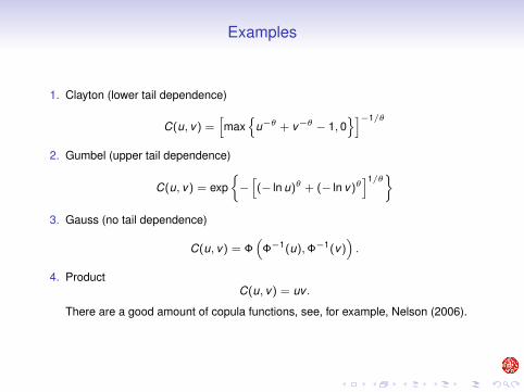
Examples

1. Clayton (lower tail dependence)

C(u, v) =[max

{u−θ + v−θ − 1, 0

}]−1/θ

2. Gumbel (upper tail dependence)

C(u, v) = exp{−[(− ln u)θ + (− ln v)θ

]1/θ}

3. Gauss (no tail dependence)

C(u, v) = Φ(

Φ−1(u),Φ−1(v)).

4. ProductC(u, v) = uv .

There are a good amount of copula functions, see, for example, Nelson (2006).

Copula

Copula-the emperor’s new clothes?THOMAS MIKOSCH (Extreme, 2005)

• There is no particular advantage of using copulas when dealing with multivariatedistributions. Instead one can and should use any multivariate distribution which issuited to the problem at hand and which can be treated by statistical techniques.

• The marginal distributions and the copula of a multivariate distribution areinextricably linked. The main selling point of the copula technology -separation ofthe copula (dependence function) from the marginal distributions -leads to abiased view of stochastic dependence, in particular when one fits a model to thedata.

• Various copula models (Archimedean, t-, Gaussian, elliptical, extreme value) aremostly chosen because they are mathematically convenient; the rationale for theirapplications is murky.

• Copulas are considered as an alternative to Gaussian models in a non-Gaussianworld. Since copulas generate any distribution the class is too big to beunderstood and to be useful. There is little statistical theory for copulas.Sensitivity studies of estimation procedures and goodness-of-fit tests for copulasare unknown. It is unclear whether a good fit of the copula of the data yields agood fit to the distribution of the data.

• Copulas do not contribute to a better understanding of multivariate extremes.• Copulas do not fit into the existing framework of stochastic processes and time

series analysis; they are essentially static models and are not useful for modelingdependence through time.

No! At least the Emperor wears socks!

A note from Paul Embrechts-Journal of Risk and Insurance, 2009

Thomas Mikosch compared the copula craze with Hans Christian Andersen’s fairy tale“The Emperor’s new clothes" where the child says “But he hasn’t got anything on!". In arecent publication, Kluppelberg and Resnick (2009), the authors end with “ReligiousCopularians have unshakable faith in the value of transforming a multivariatedistribution to its copula. For the sceptics who believe the Emperor wears no clothes(Mikosch ,2005), perhaps use of the Pareto copula convinces some of these theEmperor at least wears socks." It is my personal belief that over the years to come,research will be able to put further garments on the poor man so that eventually inHans Christian Andersen’s words we can truly say “Goodness! How well they suit yourMajesty! What a wonderful fit! What a cut! What colors! What sumptuous robes!".

Genest and Remillard-Extremes, 2006

Regretfully, he has chosen to produce a pamphlet which, written as it is in a lively butdistinctly unscientific style, clearly does a disservice to the community by “throwing thebaby out with the bathwater." While we respect his right to “ask some naive questions,"we can hardly accept that either through ignorance or malice, he depicts copula theoryas an unsubstantiated fad that leads to “a biased view of stochastic dependence."

Direct Decomposition

Based on

f (x1, . . . , xn) =n∏

j=1

f(xj | parents(xj )

),

and

f (x1, . . . , xn) = c(F1(x1), . . . ,Fn(xn))n∏

i=1

fi (xi ),

we can construct the following Bayesian model based on copulas:

f (x1, . . . , xn) =n∏

j=1

c(Fj (xj ),Fparents(j)(parents(xj )))∫c(Fj (xj ),Fparents(j)(parents(xj )))fj (xj )dxj

.

Pair Decomposition

While there is a plethora of literature on bivariate copula families (also calledpair-copula families), the range of higher-variate copula families is rather limited, seeJoe (1997, Chapter 4). Many popular bivariate copulas have no straightforwardmultivariate extension.

Based on work of Joe (1996), Bedford and Cooke (2002, The Annals of Statistics)therefore proposed a flexible way of constructing multivariate copulas that uses(conditional) pair copulas as building blocks only. The core of their approach is agraphical representation called a regular vine that consists of a sequence of trees,each edge of which is associated with a certain pair copula. This idea was furtherdeveloped by Aas et al. (2009, Insurance: Mathematics and Economics), and others.

Based on similar idea, Bauer, et al. (2011) developed the pair composition for Bayesiannetwork.

Pair-copula constructions for Bayesian network

D = (V ,E) is a DAG with vertex set V and edge set E , and define

pa(v ; w) := {u ∈ pa(v)|u < w ,w ∈ pa(v)}.

For example, for V = {1, 2, 3, 4}, we have:

pa(1; ∅) = ∅, pa(2; 1) = ∅, pa(3; 1) = ∅, pa(4; 2) = ∅

pa(4; 3) = {2}.

For the Bayesian network with continuous distributions:

f (x1, . . . , xn) =n∏

i=1

fi (xi )∏

w∈pa(v)

cvw(Fv|pa(v ;w)(xv |xpa(v ;w)),Fw|pa(v ;w)(xw |xpa(v ;w))|xpa(v ;w)

).

In our example,

f (x1, x2, x3, x4) =4∏

i=1

fi (xi ) · c21(F2(x2),F1(x1))c31(F3(x3),F1(x1))c42(F4(x4),F2(x2))

× c43|2(F4|2(x4|x2),F3|2(x3|x2)|x2)

MLE estimation

How can we derive the conditional copula, say, c43|2? In practice, we just assume thatthey are unconditional. This assumption reduces model complexity while stillencompassing a rich class of DAG copulas and has become common practice inlikelihood inference for PCCs, see Aas et al. (2009) and Haff, et al. (2010).

The log-likelihood function in our example is

log(L) =4∑

i=1

log(fi (xi )) + log(c21(F2(x2),F1(x1))) + log(c31(F3(x3),F1(x1)))

+ log(c42(F4(x4),F2(x2))) + log(c43|2(F4|2(x4|x2),F3|2(x3|x2)))

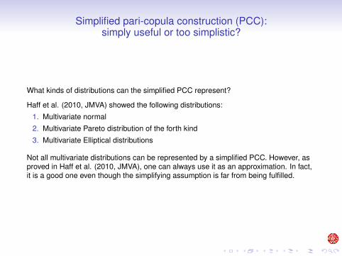
Simplified pari-copula construction (PCC):simply useful or too simplistic?

What kinds of distributions can the simplified PCC represent?

Haff et al. (2010, JMVA) showed the following distributions:

1. Multivariate normal

2. Multivariate Pareto distribution of the forth kind

3. Multivariate Elliptical distributions

Not all multivariate distributions can be represented by a simplified PCC. However, asproved in Haff et al. (2010, JMVA), one can always use it as an approximation. In fact,it is a good one even though the simplifying assumption is far from being fulfilled.

Estimation

1. Marginal distributions1.1 Joe and Xu (1996): Inference functions for marginals (IFM)1.2 Genest et al. (1995): Transform univariate marginals to uniforms

2. Estimate parameters of Copulas

After we estimate the marginal distributions, we select proper copulas to estimatetheir parameters. Note we estimate the parameters of each copula independentlyof the others.

3. Model selection

BIC or AIC

Application: Financial returns

Purpose: Modeling dependence structure of daily log-returns of DJI, DJCB, DAX,RDAX.

DJI=Down Jones Industrial AverageDJCB=Dow Jones Corporate Bond IndexDAX=German stock indexRDAX=the corresponding German corporate bond index

Data: April 3rd, 2007 to Sep. 30, 2010.

Based on the economic consideration that the German stock index is driven by its UScounterpart and that within the US and Germany corporate bond indices are driven bythe respective national stock indices. That is1=DJI2=DJCB3=DAX4=RDAX

Choose proper copulas

Aas, K. and Czado, C. and Frigessi, A. and Bakken, H. (2009) Pair-copulaconstructions of multiple dependence. Insurance: Mathematics and Economics 44,182-198.

Bedford, T. and R. M. Cooke (2002). Vines - a new graphical model for dependentrandom variables. Annals of Statistics 30(4), 1031-1068.

A. Bauer, C. Czado and T. Klein, Pair-copula construction for non-Gaussian DAGmodels (2011).