An Introduction toMicrowaves

AN INTRODUCTION TOMICROWAVES

Other Books of Interest

BP254 From Atoms to AmperesBP293 An Introduction to Radio Wave Propagation

AN INTRODUCTION TOMICROWAVES

by

F. A. WILSON

BERNARD BABANI (publishing) LTDTHE GRAMPIANS

SHEPHERDS BUSH ROADLONDON W6 7NF

ENGLAND

Please Note

Although every care has been taken with the production of thisbook to ensure that any projects, designs, modifications and/orprograms etc. contained herewith, operate in a correct and safemanner and also that any components specified are normallyavailable in Great Britain, the Publishers do not accept respon-sibility in any way for the failure, including fault in design, ofany project, design, modification or program to work correctlyor to cause damage to any other equipment that it may beconnected to or used in conjunction with, or in respect of anyother damage or injury that may be so caused, nor do thePublishers accept responsibility in any way for the failure toobtain specified components.

Notice is also given that if equipment that is still underwarranty is modified in any way or used or connected withhome -built equipment then that warranty may be void.

© 1992 BERNARD BABANI (publishing) LTD

First Published - January 1992

British Library Cataloguing in Publication DataWilson, F. A. (Frederick Arthur)An introduction to microwaves.I. Title621.3813

ISBN 0 85934 257 3

Printed and bound in Great Britain by Cox & Wyman Ltd, Reading

Preface

Read not to contradict and confute, nor to believe andtake for granted, nor to find talk and discourse, but toweigh and consider.

Francis Bacon, Of Studies

Although microwaves had been around for some time, it wasnot until 1947 that their use for cooking was introduced.Since then slowly but surely the term has become a householdword but how many households have the faintest idea of whata microwave really is? Naturally we of the electronics faithknow all about them - or do we? Just in case we are unsurehow to answer this question, this book has been written. Itsmain purpose is to ensure that microwaves are no longershrouded in mystery for we can no longer afford to beindifferent to their accomplishments since many facets of oursociety would collapse without them. For example, multitudesof telephone calls travel by microwave, the waves carry ourtelevision over land or by satellite, aircraft land safely and evenwars are won with their help.

This book is not for the expert but neither is it for thecompletely uninitiated. It is assumed that the reader hassome basic knowledge of electronics, including semiconduc-tors. There is some additional help in the Appendices forreaders who have yet to become involved in the field ofcommunications.

Although electronics is often explained with the aid ofmathematical equations for they are a concise and accurateway of expressing ideas, they tend to dishearten many would-be enthusiasts. Accordingly the temptation to indulge indetailed discussions has been avoided with long-windedmathematical reasoning giving way to a mention of the finaloutcome only.

To those of us brought up on wired -in components, thestudy of microwaves expands our way of thinking into wavetheory and the idea of electromagnetic waves propagatingthrough space instead. The use of microwaves grows inexor-ably, thus creating an ever increasing need for at least some

basic understanding of their nature.Nature may be wonderful, she controls our lives but not

man's ingenuity. We read this while surrounded by a pro-fusion of man-made radio waves, unseen and unheard until adevice fabricated from the very earth on which we live picksout the one we require. Such is radio, truly a fascinatinginvention but who can really appreciate, yet alone understand,an electromagnetic wave reversing its direction more than onethousand million times in only one second! Nevertheless asShakespeare's soothsayer said:

In Nature's infinite book of secrecyA little I can read.

Read on and for us may the little become a little more.

F. A. Wilson

Contents

PageChapter 1 - INTRODUCTION 1

1.1 Charge 1

1.2 Waves 21.3 The Electromagnetic Wave 3

1.4 Electromagnetic Radiation 5

1.5 The Electromagnetic Wave Spectrum 7

1.6 Microwaves 9

1.7 Managing Microwaves 11

Chapter 2 - MOVING MICROWAVES AROUND 132.1 Transmission Lines 13

2.1.1 Characteristic Impedance 152.1.2 Reflection and Standing Waves 172.1.3 Matching 202.1.4 Resonant Cavities 21

2.2 Coaxial Cables 232.3 Waveguides 26

2.3.1 Guiding the Wave 262.3.2 Propagation Modes 27

2.4 Antennas 292.4.1 Dipoles 292.4.2 The Focused Wave 31

2.5 Ferrites 332.5.1 Isolators 362.5.2 Circulators 362.5.3 Filters 37

Chapter 3 - MICROWAVE GENERATIONAND PROCESSING 39

3.1 Grid -Controlled Microwave Tubes 393.2 Linear Beam Microwave Tubes 41

3.2.1 Klystron 433.2.2 Travelling -Wave Tube 453.2.3 Backward -Wave Oscillator 48

3.3 Crossed -Field Microwave Devices 503.3.1 Magnetron 533.3.2 Crossed -Field Amplifiers 55

Page

Chapter 3 (Continued)3.4 Semiconductor Devices 57

3.4.1 Diodes 583.4.2 Bipolar Transistors 633.4.3 Field -Effect Transistors 643.4.4 Parametric Amplifiers 67

3.5 Mixers 70

Chapter 4 - MEASUREMENT 734.1 Frequency 734.2 Power 75

4.2.1 Barretters 764.2.2 Thermocouples 76

4.3 Attenuation 79

Chapter 5 - THE MAGIC OF MICROWAVES -COMMUNICATION SYSTEMS 81

5.1 Propagation 815.1.1 The Ground Wave 815.1.2 The Sky Wave 82

5.2 Point -to -Point Microwave Communication . . 835.2.1 Assembling the Package 855.2.2 Modulating a Microwave Carrier 865.2.3 Transmission 885.2.4 Mobile Communication 89

5.2.4.1 Frequency Considerations . . 905.2.4.2 The Cellular System 915.2.4.3 Reducing Signal Fluctuations 93

5.3 Broadcast Communication 955.3.1 Television (Terrestrial) 955.3.2 Television (Satellite) 96

Chapter 6 - THE MAGIC OF MICROWAVES - RADAR 996.1 Reflection of Radio Waves 996.2 The Radar Range Equation 1006.3 Elements of a Radar System 1056.4 Navigation and Electronic Warfare 106

Page

Chapter 7 - THE MAGIC OF MICROWAVES -HEATING 111

7.1 Charge Displacement 1127.2 Polarization 1127.3 Microwave Heating Frequencies 1147.4 A Typical Microwave Heating System 1157.5 Microwave Diathermy 117

Appendix 1 - DECIBELS 119

Appendix 2 - SIGNAL-TO-NOISE RATIO 123

Appendix 3 - MODULATION 127

Index 129

Chapter 1

INTRODUCTION

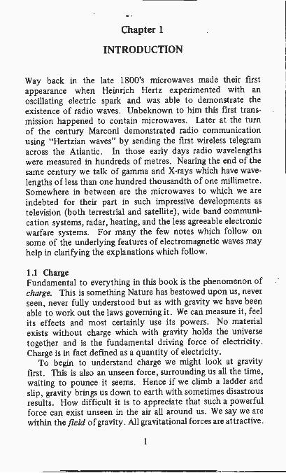
Way back in the late 1800's microwaves made their firstappearance when Heinrich Hertz experimented with anoscillating electric spark and was able to demonstrate theexistence of radio waves. Unbeknown to him this first trans-mission happened to contain microwaves. Later at the turnof the century Marconi demonstrated radio communicationusing "Hertzian waves" by sending the first wireless telegramacross the Atlantic. In those early days radio wavelengthswere measured in hundreds of metres. Nearing the end of thesame century we talk of gamma and X-rays which have wave-lengths of less than one hundred thousandth of one millimetre.Somewhere in between are the microwaves to which we areindebted for their part in such impressive developments astelevision (both terrestrial and satellite), wide band communi-cation systems, radar, heating, and the less agreeable electronicwarfare systems. For many the few notes which follow onsome of the underlying features of electromagnetic waves mayhelp in clarifying the explanations which follow.

1.1 ChargeFundamental to everything in this book is the phenomenon ofcharge. This is something Nature has bestowed upon us, neverseen, never fully understood but as with gravity we have beenable to work out the laws governing it. We can measure it, feelits effects and most certainly use its powers. No materialexists without charge which with gravity holds the universetogether and is the fundamental driving force of electricity.Charge is in fact defined as a quantity of electricity.

To begin to understand charge we might look at gravityfirst. This is also an unseen force, surrounding us all the time,waiting to pounce it seems. Hence if we climb a ladder andslip, gravity brings us down to earth with sometimes disastrousresults. How difficult it is to appreciate that such a powerfulforce can exist unseen in the air all around us. We say we arewithin the field of gravity. All gravitational forces are attractive.

1

Charges on the other hand are of two different kinds.Within an atom the protons which reside in the nucleus aresaid to have a positive charge, the electrons orbiting aroundthe nucleus carry (or perhaps are) a negative charge. Thegolden rule is:

"like charges repel, unlike attract"

so the unlike charges of protons and electrons in an atomattract each other and are responsible for keeping the atomtogether. They balance exactly, hence a complete atomexhibits no net charge. That unending power is exerted whenmany fundamental particles such as electrons get togetherbecomes evident when we pause to consider that it is theircharges which provide the force to drive the many tonnes ofan electric train.

Of interest is the fact that we measure charge in coulombs(after Charles Augustin de Coulomb, a French engineer andphysicist). If 6.242 x 1018 elementary charges (e.g. electrons)congregate together, the total charge is equal to one coulomb.The charge of a single electron is therefore 1/(6.242 x 1018)= 1.602 x 10-19 coulombs. If one coulomb of charge passesa given point in one second, one ampere of current is said toflow.

1.2 WavesThrow a pebble into a pond and the particles of water dis-placed by the pebble rise in a ring, this has to be for there isnowhere else for them to go. Then gravity pulls them down sodisplacing some of the water outside of the ring which in itsturn is compelled to rise, again to be pulled down by gravity.So the circle of waves goes on widening, driven by the energygiven up by the stone. Although the waves travel outwards itis important to note that a cork on the surface of the waterbobs up and down but does not travel with the waves, henceshowing that there is no advance of the particles of themedium in the wave direction.

A waveform is a curve showing the shape of the wave at anygiven time as plotted on graph paper or by an oscilloscope.

2

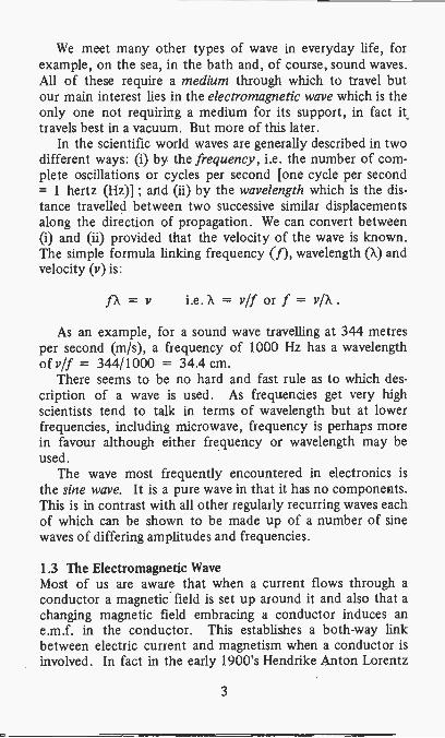
We meet many other types of wave in everyday life, forexample, on the sea, in the bath and, of course, sound waves.All of these require a medium through which to travel butour main interest lies in the electromagnetic wave which is theonly one not requiring a medium for its support, in fact ittravels best in a vacuum. But more of this later.

In the scientific world waves are generally described in twodifferent ways: (i) by the frequency, i.e. the number of com-plete oscillations or cycles per second [one cycle per second= 1 hertz (Hz)] ; and (ii) by the wavelength which is the dis-tance travelled between two successive similar displacementsalong the direction of propagation. We can convert between(i) and (ii) provided that the velocity of the wave is known.The simple formula linking frequency (f), wavelength (X) andvelocity (v) is:

fX = v i.e. X = v/f or f = v/X

As an example, for a sound wave travelling at 344 metresper second (m/s), a frequency of 1000 Hz has a wavelengthof v/f = 344/1000 = 34.4 cm.

There seems to be no hard and fast rule as to which des-cription of a wave is used. As frequencies get very highscientists tend to talk in terms of wavelength but at lowerfrequencies, including microwave, frequency is perhaps morein favour although either frequency or wavelength may beused.

The wave most frequently encountered in electronics isthe sine wave. It is a pure wave in that it has no components.This is in contrast with all other regularly recurring waves eachof which can be shown to be made up of a number of sinewaves of differing amplitudes and frequencies.

1.3 The Electromagnetic WaveMost of us are aware that when a current flows through aconductor a magnetic field is set up around it and also that achanging magnetic field embracing a conductor induces ane.m.f. in the conductor. This establishes a both -way linkbetween electric current and magnetism when a conductor isinvolved. In fact in the early 1900's Hendrike Anton Lorentz

3

changing magneticfield of

electron current

4-,c 44.a) 4 \;,.

c "or:

metal plates

- 14I-trsy.

-%%." displacement

current

changing magneticfield of

displacementcurrent

(i) a displacement current produces its own magnetic field

lines representingthe magnetic

field

II11III I 1 1 1 A

1 1 1 1 I IIIII1 1 1 1

1 1 I I

11111 1 1 1IIIII

1 4 4 4 4 1 1

A

1

(ii) simple representation of fieldslines representingelectric field at

a particularinstant

FIG. 1.1 THE ELECTROMAGNETIC FIELD

4

was able to show that both current flow and magnetism aresimply different aspects of the forces arising from charges inmotion. We need to go one stage further however to under-stand that a changing electric field can give rise to a displace-ment current in an empty space where no conductor is present.In Figure 1.1(i) are two metal plates to which an alternatingpotential is applied, hence a changing electric field arisesbetween them. James Clerk Maxwell in the 1860's was thefirst to suggest that a changing electric field could producewhat he called a displacement current even in empty spaceand as shown in the figure, that this is just as capable ofproducing a magnetic field as the current in a conductor. Toavoid some heavy -going mathematics, we must accept thatdisplacement current arises from the fact that an appliedelectric field creates an electric flux through any dielectric,even space and that the current is given by the rate of changeof flux with respect to time. It can also be shown to be pro-portional to the rate of change of the electric field strength sohere is a kind of Ohm's Law relationship but referring tochanging quantities only.

Using our most convenient way of representing a field, i.e.by arrowed lines, (i) of the figure can be shown as in (ii). Thetwo fields are at right angles.

As the generator in (i) reverses polarity so the arrows on thefield lines in (ii) reverse in direction. When the combination ofelectric and magnetic fields is forced to move outwards we willsee from the next section that an electromagnetic wave isproduced.

1.4 Electromagnetic RadiationElectromagnetic radiation occurs when a charge is made tooscillate quickly in anything but we use as an example anantenna wire. A changing electric field ensues which as shownin Section 1.3 sets up a changing magnetic field at right anglesto it. In turn the magnetic field creates another changingelectric field at right angles but in the opposite direction to theoriginal one. This second electric field produces a furthermagnetic field and so on. Thus the two fields are linked andthey reinforce in such a way as to keep one another going.Perhaps the simplest way of looking at the process is to

5

consider the energy transferred from the oscillatory current tothe fields. As the fields collapse this energy would normallybe returned to the wire. However, if the charge polarity hasreversed before the fields have fully collapsed, all of the fieldenergy cannot be returned because new and opposite fields arein the way. The original fields are therefore forced away fromthe wire and together they form a train of waves travellingoutwards from the antenna at a speed determined by thesurrounding medium. For any medium the velocity is given by:

v = ue) metres per second

where I/ is the permeability and e the permittivity of themedium.

For free space (i.e. a vacuum containing no nearby objects),the permeability is 4ir x 10-7 and the permittivity 8.854 x10' so using c for the free space velocity, this works out to:

c = 2.998 x 108 or very nearly 3 x 108 m/s

which is the figure used generally.For other media v is lower because both permeability and

permittivity are greater than 1. For air, however, the valuesare so close to 1 that the velocity is almost identical with c.

We need to be able to quote the directions of the fields ofa particular electromagnetic wave, i.e. to state the wavepolarization. It is only necessary to specify one of the fieldssince the pair are at right angles. It has generally been agreedto use the electric field for this purpose so a horizontallypolarized wave has its electric field lines horizontal (magneticvertical) and vice versa. Accordingly the wave shown inFigure 1.1(ii) is a horizontal one. The arrows reverse directionat each half -cycle of the wave. A wave may not be trulyvertical or horizontal, many things can happen to it in itstravels or it may be deliberately radiated at some other angle.Another much used polarization in microwave transmission iscircular. In this case the electric and magentic fields remain atright angles to each other but now the pair continually rotate.We may need to know which way round they are going so ifwe look towards an oncoming wave, then a clockwise rotation

6

is described as positive or right-handed and anticlockwise asnegative or left-handed.

The plane of polarization is the plane which contains boththe direction of the electric field and the direction ofpropagation.

Mode is a term which describes the form in which anelectromagnetic wave is propagated, more specifically itrelates to the electric and magnetic field patterns existing in awaveguide. Many of the patterns are distinguished by codenames, these are discussed in greater detail in Section 2.3.

When the fields as shown in Figure 1.1(ii) vibrate at rightangles to the direction of propagation, the wave is describedas transverse. Electromagnetic waves in free space and air arenormally transverse and are called TEM waves (transverseelectric and magnetic).

1.5 The Electromagnetic Wave SpectrumIn Section 1 is an indication that the range of wavelengthsseems to be never-ending, this range is generally called theelectromagnetic spectrum, running from the longest wavesof radio to the tiny wavelengths of gamma and cosmic rays.Within the spectrum are shorter ranges which are classifiedby their usage. A comparatively short but absolutely essentialrange is near the centre, these wavelengths give us light, i.e.they are capable of stimulating the light receptors of the eye.Figure 1.2(i) shows at the top the full wave spectrum but itmust be appreciated that there are no clear-cut divisionsbetween the various ranges or bands, they merge into oneanother. Moreover there is little general agreement on theband limits except for the internationally agreed radio -frequency bands shown near the bottom of (i). These are:

Band Frequency Frequency Letter MetricNo. Range Description Designation Subdivision

4 3-30kHz Very Low VLF MyriametricWaves

5 30-300kHz Low LF KilometricWaves

6 300kHz-3MHz Medium MF HectometricWaves

7

1cm

11

1mm

wav

elen

gth

410

-410

-610

-810

-10

10-1

2(m

etre

s)10

102

1lo

-2

10-1

41

freq

uenc

y104

(her

tz)

1

10K

Hz

1 114

long

T

1

-

I8

101

i s

1MH

z

108

I10

10

1GH

z

1012

1014

infr

a-re

d

II

1016

1018

x-ra

ys

f10

2010

22

gam

ma

cosm

icra

ys

ultr

ash

ort w

aves

shor

t

UH

F S

HF

EH

F

visi

ble

spec

trum

ultr

avio

let

rays

..."

med

iumok

N, .-

I"br

oadc

ast

radi

o w

aves

VH

F

VLF

I LF

IMF

IH

FIIII mic

row

aves

(i)th

e co

mpl

ete

spec

trum

I

(ii)

the

mic

row

ave

rang

e3m

1.33

m30

cm3c

m3m

m

1

100M

Hz

225M

Hz

1GH

z10

GH

z10

0GH

zV

HF

UH

FS

HF

EH

FF

IG. 1

.2E

LEC

TR

OM

AG

NE

TIC

WA

VE

SP

EC

TR

UM

Band Frequency Frequency Letter MetricNo. Range Description Designation Subdivision

7 3-30MHz High HF DecametricWaves

8 30-300MHz Very High VHF Metric Waves

9 300MHz-3GHz Ultra High UHF DecimetricWaves

10 3-30GHz Super High SHF CentimetricWaves

11 30-300GHz Extremely EHF MillimetricHigh Waves

[1 MHz = 10' Hz, 1 GHz (gigahertz) = 109 Hz]

1.6 MicrowavesThe prefix micro is not used as elsewhere in electronics toindicate one millionth; coming from the Greek mikros itsimply means small, hence microwaves are those of relativelysmall (short) wavelength. They are certainly short whencompared with long waves of between 1000 and 2000 metres.It is obvious from Figure 1.2(i) that waves considerablysmaller exist but microwaves were so named when the poten-tial utilization of wavelengths less than about one metre wasonly just beginning. At the very bottom of (i) of Figure 1.2is shown the position of the microwave band and this isamplified in (ii). This is a commonly used one but otherranges than this are to be found and there is appreciablevariation. The one shown extends from 1.33 metres down to3 mm (225 MHz -> 100 GHz). As an indication of the degreeof variation, here are a few examples taken from modernpublications:

50 cm -> 1 mm, 100 cm -> 1 mm, 30 cm -> 0.03 mm,less than 3 m, less than 20 cm, less than 1 cm.

The band we have chosen is subdivided with letter designa-tions as follows:

9

P band 1.33 m - 76.9 cmL band 76.9m - 19.3 cmS band 19.3 m -> 5.77 cmX band 5.77 m -+ 2.75 cmK band 2.75 cm -> 8.34 mmQ band 8.34 cm -). 6.52 mmV band 6.52 cm - 5.36 mmW band 5.36 cm -+ 3.00 mm

There is also a C band running from 7.69 cm to 4.84 cm.These bands are again subdivided and are frequently quoted

in radar and satellite technology although again, there is con-siderable variation, especially with the latter.

Some major developments in microwave technology havebeen:

(i) the discovery that above about 1.5 GHz microwavesbehave in many respects as do light waves. Hence thesemicrowaves can be reflected as can those of light;

(ii) by such reflections, when the wavelength is sufficientlyshort the wave can be transmitted in a hollow metaltube or waveguide. The wave can be pictured as bounc-ing from wall to wall along the guide;

(iii) the development in the late 1930's of the klystron, adevice capable of generating a continuous supply ofmicrowaves. This development advanced microwavetechnology considerably;

(iv) at very short wavelengths microwaves exhibit proper-ties similar to those of infra -red radiation which asFigure 1.2 shows is next door in the spectrum. Infra -redrays are those which produce heat so it was found thatmicrowaves could also be used for heating.

Also it is clear that microwaves have the great advantageover waves of lower frequency in the width of frequencyspectrum they offer for communication purposes. From therange shown in Figure 1.2, if we take, say 30 cm to 3mm asan example, some 99 GHz bandwidth is there, i.e. 99 timesthat already provided by all of the lower broadcast frequenciestogether which because of the many requirements thrust uponthem are very crowded indeed (bandwidth is considered in

10

more detail in Appendix 3). Another, perhaps naive way oflooking at this is to consider that if the modulation frequenciesoccupy the same percentage of the carrier frequency in allcases (hardly true but useful for demonstrating the point),then the bandwidth which can be carried at 10 GHz is 100times that at 100 MHz. The question immediately arises as towhy not go still higher in frequency, i.e. into the infra -redregion, but then losses when propagating through the atmo-sphere become excessive (we know only too well what happensto light in a mist or fog). So for broadcast and for point-to-point communication, microwaves have much to offer.

It would have been gratifying to have included in microwaveachievements their use in medical electronics. Unfortunatelya cursory examination of present techniques shows that atpresent ultrasonics (sound frequencies above about 20 kHz),X-rays and nuclear rays are in the greatest demand, uses formicrowaves are few, one of interest however is mentioned inSection 7.5.

1.7 Managing MicrowavesCircuit techniques used for equipment working at frequenciesbelow the microwave range are unlikely to be successful withmicrowaves for several reasons, one obvious one being that ofregeneration causing instability. Adjacent wires of conven-tional wiring having only a single picofarad of capacitancebetween them are in fact coupled by a capacitive reactance aslow as 16 ohms at 10 GHz, unwanted energy is thereforeeasily transferred. Also wire and component inductancesdevelop large unwanted voltages which similarly create havoc.In addition all electric circuits carrying an alternating currentradiate energy with a radiated field strength which variesdirectly as the frequency. At normal broadcast wavelengthsthis is low enough to be of little consequence but at micro-wave frequencies radiation from metal parts such as wires andcomponents is appreciable. Such losses cannot normally betolerated within equipments hence foi microwaves differenttechniques have been, and still are being developed.

Much use is made in microwave technology of transmissionlines, coaxial cables and waveguides. Short-circuited lengths oftransmission line are also used to provide reactances. With the

11

drive for miniaturization microstrip transmission lines ofwidth 4 mm or less have come into use. For such a smallcomponent a relationship with the open -wire transmission lineor coaxial cable may seem tenuous but at such short wave-lengths this is the order of dimension required. We might sumthis up by saying that for microwaves the lumped constantapproach generally effective for circuit analysis at the lowerfrequencies is replaced by electromagnetic wave _theory inwhich transmission lines play a major part.

Advanced semiconductor technology now forms the basisof many microwave devices although magnetrons, klystronsand travelling -wave tubes still hold considerable sway; theseare considered in detail in Chapter 3.

An interesting microwave device is the ferrite which, totake a single example, when biased by a suitable magnetic fieldis capable of phase -shifting a microwave and hence can be usedas an isolator in that the wave travels in one direction througha device but not in the reverse direction.

These few examples of devices and techniques show thatnot only are we capable of handling the very high frequenciesof microwaves but that much of the experience gained isleading to the development of devices for special applicationshitherto unheard of.

12

Chapter 2

MOVING MICROWAVES AROUND

Any attempt to get to grips with microwave generation andtransmission must come to naught unless we have someappreciation of transmission lines and waveguides. Both ofthese are subjects on their own and as might be expected, fullanalysis becomes highly mathematical and is therefore not forus here. All we need is to become acquainted with just a fewof the elementary principles so that we can form pictures inthe mind of how energy travels along lines as waves and thento realize that at microwave frequencies just any transmissionline will not do, it has to be related to the length of the wave.We will also find that for waveguides the normal losses due toconductor resistance, insulation losses and radiation areinsignificant.

2.1 Transmission LinesFirstly when does a circuit become a transmission line? Figure2.1 shows at (i) a generator with its nearby load - no prob-lems here because Ohm's Law is effective with no stringsattached. At (ii) the generator and load are separated, it maybe over a distance of many kilometres or at very high fre-quencies a few millimetres. Electrical energy moves betweengenerator and load in a form of wave motion and it wouldseem that both the time it takes to reach the load and thedistance the load is from the generator are involved. We canget some proof of this by accepting the mathematical formulafor the voltage V1 developed across the line at a distance 1from the generator. Suppose that the generator applies avoltage V to the line, then:

= V cos w(t + )3l/w)

where t is the time of travel, w = 2irf and 13 =Looking more closely at the term (31/co, this can be reduced

to 1/v where v is the velocity of signal propagation, hence it isclear that length besides time and velocity control the value of

13

m:

load,R

L

(i) generator with nearby load

transmissionline

6

/

(ii) generator with a remote load

FIG. 2.1 CONNECTING A GENERATOR TO A LOAD

V1. It is perhaps possible now to appreciate the main differ-ences between "normal" circuit design and that for micro-waves. With the normal circuit it does not matter electricallyhow large or small a resistor is provided that its characteristicsare those required, similarly with capacitors and inductors.On the other hand, because as we have seen in Section 1.7that conventional techniques cannot be used with microwaves,it is clear that at these frequencies dimensions become impor-tant and must often be related to the wavelength. Thisfrequently happens to be a useful feature for at such shortwavelengths even transmission lines may be small enough to betreated as discrete components.

14

For those whose transmission line theory has seen betterdays, the next two sections contain some useful reminders.

2.1.1 Characteristic ImpedanceFirst let us imagine a line consisting of two conductors dis-appearing off to infinity. Application of a signal to theconductors (or transmission line) would result in a wavetravelling along the line and going on for ever, the line simplyacting as a resistance because it can continuously absorbpower. This in fact defines the characteristic impedance of atransmission line, i.e. the impedance looking into an infmitelength of a line. It is normally designated by Zo . Figure 2.2shows at (i) that Zo is determined straightforwardly from thevalues of V and I.

Next suppose that a short length is cut off at the near -endof the line as in (ii) so creating terminals 3 - 6. Lookingdown the line from terminals 5 and 6 the impedance is stillZo because the infinite nature of the line is unaffected, there-fore by connecting an impedance Zo to terminals 3 and 4 asin (iii) the impedance looking into terminals 1 and 2 is identicalwith that in (i), that is, the short length of transmission line in(iii) behaves as though it were infinitely long. This makessome sense except that we could not have had an infinite lineon which to measure Zo in the first place, it can however beshown that certain measurements can be made on a shortlength of line by which Zo can be determined.

Looking more closely at a short length of the line, it can beseen to have four primary coefficients (i) the resistance of theconductors (R), (ii) inductance (L - even a straight wire hasinductance), (iii) capacitance between the two conductors (C)and (iv) there is a loss due to the conductance of the insulatingmaterial between the conductors, the coefficient is known asthe shunt conductance (G). Usually these four values arequoted per metre of line length. Standard transmission linetheory arrives at the conclusion that:

Zo =G + jo)C

15

near

-end

1

(i)m

easu

rem

ent

0o

2

tran

smis

sion

line

0

shor

t len

gth

cut o

ff

13

50

ob

24

zo-1

"o-

-0o

(ii)

shor

t len

gth

cut o

ff at

nea

r -e

nd6

Z0

13

(iii)

shor

t len

gth

term

inat

ed in

Zo

- fa

r-en

d

to in

finity

to in

finity

FIG

. 2.2

CH

AR

AC

TE

RIS

TIC

IMP

ED

AN

CE

where w = 2rf and f is the frequency under consideration. j isthe standard "operator" used in circuit analysis to indicate aphase difference of 90°.

In practical microwave circuits it is frequently possible toassume that a line is lossless, i.e. that R and G are both zerowhereupon Z0 is more simply expressed as NAL/C).

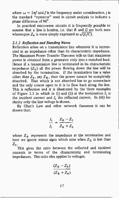
2.1.2 Reflection and Standing WavesReflection arises on a transmission line whenever it is termin-ated in an impedance other than its characteristic impedance.The Maximum Power Transfer Theorem tells us that maximumpower is obtained from a generator only into a matched load.Hence if a transmission line is terminated in its characteristicimpedance (Z0) all the power flowing down the line will beabsorbed by the termination. If the termination has a valueother than Z0, say ZR, then the power cannot be completelyabsorbed. That which is not absorbed has to go somewhereand the only course open to it is to flow back along the line.This is reflection and it is illustrated by the three examplesof Figure 2.3 in which in (i) and (ii) at the termination 4 isthe incident current and 4 the reflected current. In (iii) forclarity only the line voltage is shown.

By Ohm's Law and other network theorems it can beshown that:

4 ZR - zo

ZR Zo

where ZR represents the impedance at the termination andhere we ignore minus signs which arise when ZR is less thanZ0 .

This gives the ratio between the reflected and incidentcurrents in terms of the characteristic and terminatingimpedances. The ratio also applies to voltages.

(ZR - zo)

(ZR + zo)

17

transmissionline`

A/4 X/4 X/4 X/4 a/4 irZo) 4. J. .4.

/. (

\'

I /

I '1 \ I. 1max

I I %

-1.

I\ = /. + /r1

1 I

I I \ I...

ZR

I I/ I

(i) mismatched line (Z R*Zo)

voltageantinode

T

/ = /. -/m n r

A/4 /r (= /i)I I 14-.4

. short -IV/

I 0 i-circuit1,ax

I /m = 2/:

/min = °

(ii) short-circuited line (ZR = 0)

A/2 Vr(= Vi)

I oI 0

\ I/ VmaxI / = 2 Vi

0node VmIn =

(iii) open -circuited line (ZR =cc)

open--circuit

FIG. 2.3STANDING WAVES ON A TRANSMISSION LINE

18

is called the reflection coefficient (symbol r, but p may alsobe used).

The graphs in the figure show line voltages and currents andas in all cases of mismatch, the current and voltage maximaand minima occur at the same points along the line. Thewaves shown are known as standing waves, having points ofminimum voltage with maximum current and vice versa. Thepoints of zero voltage are known as nodes, of maximum volt-age they are called antinodes. The nodes are exactly half awavelength apart as are the antinodes. To us this is a mostinteresting feature of a mismatched transmission line forirrespective of the power sent down the line, when thedistant end is short-circuited or open -circuited, there arepoints half a wavelength apart where no voltage (or current)can be measured even though both incident and reflectedwaves are travelling past. We can see also from the figure thatthe impedance of the line varies from zero when the voltage iszero but the current is maximum to infinite when the oppo-site applies with appropriate values in between. This isextremely useful for it allows us to cut short lengths oftransmission line to load or transform impedances, with dueregard to frequency of course (see Sect.2.1.3).

The ratio of maximum to minimum voltage on a trans-mission line carrying a standing wave is known as the standingwave ratio. We usually refer to the voltage and call it thevoltage standing wave ratio (vswr). The maximum value(Vmax) of a standing wave in terms of the reflectioncoefficient (r) follows from:

Vmax = Vr = Vi(1 r) since r = VrIVi

also the minimum value:

Vmin = V, -Vr = V,(1 - r)

hence:Vmax 1 +rvswr = -=Knin 1 -r

19

from which:

reflection coefficient, r -vswr - 1

vswr + 1

The vswr is an extremely useful parameter for use in theanalysis of microwave circuits, especially in that once itsvalue is known many other transmission line relationships canbe calculated from it.

2.1.3 MatchingFrequently it is found that a transmission line load does nothave an impedance equal to the characteristic impedance ofthe line itself, a typical example of this is an antenna whichhas an appreciable reactance and is connected to a main feederof resistive characteristic impedance. It is important to reduceor eliminate resulting reflections and therefore high vswr's onthe feeder. For these and many other mismatched conditionsit is possible to add or interpose a transmission line section tomatch the two impedances or perhaps merely to neutralize or"tune out" antenna reactance. This is the process of matchingto appreciate which we must first look more closely at how theinput impedance of a mismatched transmission line varieswith line length.

Figure 2.3 shows how the voltage and current along a lineare dependent solely on the load impedance and it is thiswhich determines their values at the point of connection. Atany point on the line therefore the impedance is simply V//but note that there is a phase difference between them. Thishighlights one of the important features of mismatched trans-mission lines which is that the impedance conditions for thewhole line are determined at the far -end of the line and thatthe impedance across the line is repeated along the line at half -wavelength (X/2) intervals. The input impedance of a line anexact number of half -wavelengths long is therefore alwaysequal to the load impedance irrespective of the line character-istic impedance. However, this repetitive condition is clearlyfrequency dependent for it can only occur at those frequenciesat which a particular length of line is an exact number of half -wavelengths long.

20

Moreover, it can be shown that because of the phasedifferences between V and I, quarter -wavelength sections ofline have capacitive or inductive reactances depending onwhether they are open or short-circuited at the far -end.

All the features of the mismatched transmission line abovehave considerable usage in microwave technology for at suchfrequencies, wavelengths are short enough for transmissionlines with mismatched terminations to be practicable. As anexample, at a medium wave broadcast wavelength of 500 ma quarter -wavelength line is 125 metres long, whereas at, say,1 cm it is a mere 2.5 mm. Both have the same electricalcharacteristics at their chosen frequencies but there is littledoubt as to which is the more functional. Again we see howspecial techniques are available with microwaves.

2.1.4 Resonant CavitiesStanding waves are also the basis of 'cavity resonators. If awaveguide which is one half of a wavelength long is closed atboth ends it then becomes a closed structure bounded byconducting walls. If a signal at the appropriate frequency isinjected into it, a standing wave pattern is generated and infact the cavity can then be considered as the microwaveequivalent of a high -Q parallel resonant circuit. For lumpedconstant resonant circuits (i.e. inductor and capacitor)reactance is required but resistance is not because it createspower losses. The quality factor or Q is the ratio betweenthem. At microwave frequencies, however, it is better toconsider Q as the ratio of the energy stored in a device to theenergy dissipated over a specified time interval (e.g. one cycleof oscillation). In practical resonators the energy dissipatedper cycle is small compared with the energy stored andtypically Q may be many thousands when the cavity is unload-ed but when couplings are added (see Sect.2.3.2), the Q fallsto a few hundreds. It is lower if a dielectric other than air isused but increases as the conductivity of the metal wallsincreases. The simplest of cavities is a cylinder with itsdiameter equal to the length so that a single half -wave patternis set up in each of the three directions.

If the length of transmission line (coaxial or waveguide) is1, then resonance of the cavity occurs when:

21

(i) type in common use

outerconductor

outerconductor

innerconductor

length ofmean path2rT(R + r)

2(II) path of non-TEM modes

FIG. 2.4 COAXIAL CABLE

22

I= nx Xg/2

where n is an integer. Ag is the wavelength in the resonator,not the wavelength in free space. It can be calculated from thefree space wavelength, A, the cut-off wavelength, ko and therelative permittivity of the dielectric (if not air).

Many other resonator shapes and modes are employed as isseen later.

2.2 Coaxial CablesAn extremely useful type of transmission line for use withmicrowaves is the coaxial cable. The type in general use hasone conductor shielding the other as sketched in Figure 2.4(i),the outer conductor being woven copper braid with the centreconductor kept in place, for example by polyethylene discs.Cable size naturally depends on its power handling capacity.

The characteristic impedance can be calculated by substitu-tion for L and C in the approximate formula Zo = NAL/C) andthis results in:

Z0 138 logio(R1r)

in which R is the inside radius of the outer conductor, r isthe radius of the inner conductor and it is assumed that thepermittivity of the dielectric (mostly dry air) = 1. See (ii)of Figure 2.4. Generally values for Zo range between 50and 100 ohms non -reactive.

It is important to avoid transmitting at a wavelength whichallows additional unwanted modes to propagate. We canimagine from Figure 2.3 that a length of transmission lineone wavelength long turned around on itself so that the endis connected to the beginning (i.e. in a circle) is in fact anopen -circuited line and therefore is capable of sustainingstanding waves, if provided with a small amount of energyfrom the main wave. This is a condition which can arise with-in the dielectric of a coaxial tube, the length of the unwantedtransmission line being equal to the mean of the circumferencesof the inner and outer conductors as shown in (ii) of thefigure, i.e. 2ir x (R + r)/2. Not only can this condition arisefor a path length of A, but also for multiples of it.

23

couplingflange

(for boltingsections:ogether)

0. I 0r

(77z7rz zzzzt

path ofwave

Oi = angle of incidence

Or = angle of reflection

ei = 9r

guide

rectangular waveguide

metal wallsof guide

dry air

(ii) zig-zag path of wave in a guide

FIG. 2.5 WAVEGUIDES continued

24

X/2

..1

I II I I

%

I I-, I__.../

I I

I

I I

II

iI

f-_, Ii r*--

1

t I,_ i

1 )----I

1

II

I I

,

I I

I I

I I

I

1

I

i

/--I ""

I

iI I I I I I I

1 1 r V I qr t I A Ai A 4 A A A1 V J

continued

l'ItX/2

lines of electric field

lines of magnetic field

(iii) fields in a TE io mode

25

Accordingly a TEM wave (Sect.1.4) being transmitted alonga coaxial cable will encounter interference and suffer loss ifsuch parasitic non-TEM modes are set up in the dielectric,generally therefore cables are operated below the frequency atwhich:

7r(R + r)Xc -

n

where X, is the cut-off wavelength and n = 1, 2, 3, . . . Thislimits the use of coaxial cable to around 3 GHz (10 cm) abovewhich waveguides take over.

2.3 WaveguidesOmitting the centre conductor of a coaxial cable gives thecircular waveguide. This is a tubular metal guide in which theelectromagnetic wave is confined rather than propagating free-ly in space. Usually the dielectric is dry air. However, wave -guides are more frequently found with rectangular cross-section, an example is shown in Figure 2.5(i).

2.3.1 Guiding the WaveJames Clerk Maxwell first developed the electromagnetictheory of light which then led directly to the discovery ofradio waves. Some of his work relates to the boundaryconditions which are present when electric and magnetic fieldstravel through one material bounded by another. This may bebetter appreciated if we recall the principles of optical reflec-tion from our schooldays, remembering that light and micro-waves are both electromagnetic waves differing only inwavelength, hence they observe the same laws of reflection atsuitable conducting surfaces. Briefly, when light enters amore dense medium its velocity falls resulting in a change ofangle of the wavefront at the surface (except at 90°). This isrefraction and as the angle of incidence (with the normal) ofthe wave increases, there is a point at which the wave cannotbe refracted but undergoes total internal reflection, so forexample, with glass the surface behaves as a perfect mirror.

26

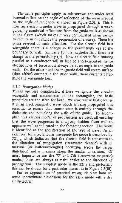
The same principles apply to microwaves and under totalinternal reflection the angle of reflection of the wave is equalto the angle of incidence as shown in Figure 2.5(4 This ishow an electromagnetic wave is propagated through a wave-

guide, by continual reflections from the guide walls as shownin the figure (which makes it very complicated when we tryto picture in our minds the progression of a wave). There is aphase reversal at each reflection. For the electric field in awaveguide there is a change in the permittivity (e) at theboundary or wall. Similarly for the magnetic field there is achange in the permeability (µ). Now an electric field runningparallel to a conductor will in fact be short-circuited, henceelectric lines of force must always be at an angle to the guidewalls. On the other hand the magnetic field will create surface(skin effect) currents in the guide walls, these currents deter-mine the waveguide loss.

2.3.2 Propagation ModesThings are less complicated if here we ignore the circularwaveguide and concentrate on the rectangular, the basicprinciples are the same for both. We now realize that becauseit is an electromagnetic wave which is being propagated it isessential to ensure that transmission is entirely through thedielectric and not along the walls of the guide. To accom-plish this various modes of propagation are used, all ensuringthat the wave progresses in a zig-zag fashion from wall toopposite wall as indicated in the foregoing section. The modeis identified in the specification of the type of wave. As anexample, for a rectangular waveguide the mode is described byTEmn which indicates that the electric field is transverse tothe direction of propagation (transverse electric) with mmaxima (or half -wavelengths) occurring across the largerdimension and n maxima along the smaller dimension. Ofmost importance are the TE and TM (transverse magnetic)modes, these are always at right angles to the direction ofpropagation. The simplest mode is the TEio and pictoriallythis can be shown for a particular instant as in Figure 2.5(iii).

For an appreciation of practical waveguide sizes here aresome approximate dimensions for the TE10 mode with a dryair dielectric:

27

to carry 3 GHz (X = 10 cm)to carry 12 GHz (X = 2.5 cm)to carry 100 GHz (X = 3 mm)

7.5 cm x 4 cm2.2 cm x 1.2 cm4.0 mm x 2.5 mm.

Each transmission mode has a lower limit to the frequencywhich can be propagated. For any transmission line there is apropagation coefficient which expresses the rate at which thecurrent falls as the wave progresses along the line or in thiscase, along the waveguide. Clearly this is a complex quantityand for a lossless transmission line the propagation coefficientmust be purely imaginary for there to be no attenuation, onlychanges in phase. This is not practicable for as we see inSection 2.3.1 there must be some loss. Nevertheless for theTE10 mode, working from the formula for the propagationcoefficient, it can be shown that the frequency of cut-off forany particular rectangular waveguide of internal dimensionsx (larger) and y (smaller):

/Co = -2 f(m/x)2 (nlY)

where c is the velocity of electromagnetic waves in space.This is for an air dielectric, for any other the formula

becomes more complicated because the permittivity andpermeability must also be taken into account. For the TE10mode m = 1, n = 0, therefore with air dielectric, theoretically:

"'co = c12x xec. = 2x

and in practical rectangular guides this is found to be approxi-mately so but remember this is for the TER, mode only.

An electromagnetic wave can be inserted into a waveguideusing either a voltage driven probe (e.g. by extending thecentre conductor of a coaxial cable into the end of the guide)or by a current carrying coil. The desired mode of trans-mission depends on the alignment of the probe or coil withinthe guide. A wave is extracted from a waveguide by a similararrangement. Certain microwave oscillators may be coupledto a waveguide by a special design of mount so that energy istransferred and in the correct mode.

28

2.4 AntennasWhen transmitted by coaxial cable or waveguide the microwavesignal may be regarded as captive and it is destined to emergeat the end of the line only. More generally transmission is viaa radio path in the atmosphere or space in which the wave is

. less constrained or may even be broadcast. For radio trans-mission there are the inevitable antennas (aerials), one fortransmitting into the radio path and one or more for receivingfrom it. There is a multitude of different antenna systemseach depending on frequency, requirement and the inventive-ness of the designer. Even for microwaves the subject is wide-ranging and includes such types as pyramidal horn, spiral andslotted. However, we can usefully reduce the range to twotypes only, both of which are more easily understood and infact are those most commonly used. These are the dipole,confined mainly to the UHF band (Fig.1.2) and the parabolicwhich takes over at frequencies above this. Generally theseantennas are reciprocal in that their basic properties are similaron both transmit and receive, also they can be designed to behighly directional.

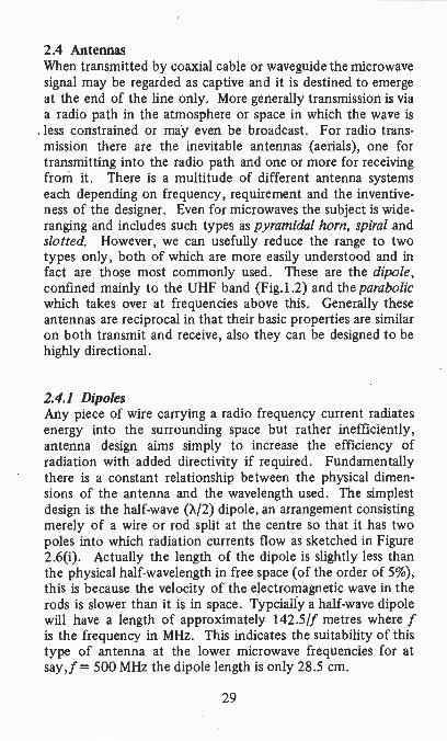
2.4.1 DipolesAny piece of wire carrying a radio frequency current radiatesenergy into the surrounding space but rather inefficiently,antenna design aims simply to increase the efficiency ofradiation with added directivity if required. Fundamentallythere is a constant relationship between the physical dimen-sions of the antenna and the wavelength used. The simplestdesign is the half -wave (X/2) dipole, an arrangement consistingmerely of a wire or rod split at the centre so that it has twopoles into which radiation currents flow as sketched in Figure2.6(i). Actually the length of the dipole is slightly less thanthe physical half -wavelength in free space (of the order of 5%),this is because the velocity of the electromagnetic wave in therods is slower than it is in space. Typcially a half -wave dipolewill have a length of approximately 142.5/f metres where fis the frequency in MHz. This indicates the suitability of thistype of antenna at the lower microwave frequencies for atsay, f = 500 MHz the dipole length is only 28.5 cm.

29

0

appr

oxX

/2

cond

uctin

gfo

lded

rod

dipo

le

(rot

ated

thro

ugh

90°

it be

com

es a

horiz

onta

l dip

ole)

coax

ial

cabl

e

(i)ve

rtic

al d

ipol

e

elec

tron

flow

tran

smitt

er

refle

ctor

coax

ial

dow

n-le

adsu

ppor

ting

mas

tinco

min

gw

ave

dire

ctor

s

(iii)

a 4-

elem

ent Y

agi r

ecei

ving

ant

enna

\\

II

I1

elec

tron

II

I'

flow

: \\ \

\1

II

I\\1

ili

t t t

1t

--31

,../

///

Ilin

es o

fIr

......

..,,,.

.,,,

elec

tric

flux

II

I

/ //

1

II

I,

,

radi

ore

ceiv

er

(ii)

radi

o tr

ansm

issi

on u

sing

dip

ole

ante

nnas

FIG

. 2.6

DIP

OLE

AN

TE

NN

AS

II

I

Recalling that the lines of an electric field are arrowedaccording to the direction in which a free positive chargewould move, (ii) of the figure shows pictorially the sequenceof events between a transmitter and receiver at a particularinstant. Only the electric field is shown, for clarity themagnetic part of the electromagnetic wave is omitted.

Much can be done to enhance the performance of theelementary receiving dipole especially by the Yagi system(after two Japanese engineers, H. Yagi and S. Uda) whichincreases the gain and improves directivity. Yagi antennashave proliferated on our roofs since UHF television trans-missions began and one has only to look at them to seewhether the electromagnetic wave for the particular area ishorizontally or vertically polarized. Figure 2.6(iii) shows a4 -element array with one reflector and two directors (manymore are frequently used). These extra rods are excited bythe oncoming wave and their spacings from the dipole aresuch that they re -radiate energy to arrive at the dipole in thedesired phase. A folded dipole is shown, this has the effectof increasing the bandwidth and raising the antennaimpedance.

For transmitters, dipole systems may also be used, usuallyseveral dipoles are connected together in parallel in a stackedarray, spaced and fed so that their outputs are all in phase.

2.4.2 The Focused WaveWe are reminded in Section 1.6 that frequencies in the SHFrange have wavelengths so short that in many respects theycan be handled as for light waves. Just as a searchlight canfocus a powerful light at its centre into a narrow parallelbeam so equally a parabolic antenna focuses a microwavesignal into a narrow beam. Practically all of the power isconcentrated in the beam and none is lost elsewhere. At thereceiving end a similar parabolic antenna receives the beamand focuses it onto a central waveguide. This is illustrated inFigure 2.7(i) with (ii) reminding us of the basic features of theparabola. The shape is that seen when a cone is sliced parallelto its side and we ought to be conversant with the generationof a parabolic curve because it features so prominently inmicrowave radio systems.

31

metal parabol creflector

from transmitter

y

vertex 0

-2

narrowmicrowave

beamI

to receiver

unidirectional point-to-point microwaveradio transmission

tangent at P

incomingAAAmicrowave

O

\ normalat P

principal axisF 4 6 8 10 x

for all parabolas y = -± 2 FT( (here ais chosen as 2).

(ii) essential features of the parabola

FIG. 2.7 THE PARABOLIC ANTENNA

32

Referring to (ii) of the figure, it can be shown that for anyelectromagnetic wave arriving parallel to the principal axis, aswith light reflected by a mirror, the angle of incidence withthe normal is equal to the angle of reflection (0 in the draw-ing). By repeating the construction shown as P moves aroundthe curve it can be demonstrated that all parts of the wave arereflected towards the focus F. F is chosen in the design pro-cess and is situated on the principal axis at a distance a fromthe vertex. Equally a wave generated at F will be reflectedalong a path parallel to the axis. However, not all microwavedish -type antennas are of the true parabolic shape. A practicaldifficulty with the parabolic is that the horn -like device whichmust be located at the focus for delivering the electromagneticwave in the case of a transmitting antenna or for collecting thewave on a receiving antenna, is itself within the path of thefree wave and therefore to some extent reduces the effectivearea of the dish. Accordingly designs are available in whicheither the wave is focused to a lower point so that the deviceis no longer in the way or a second reflector is added to guidethe wave to the centre of the main dish. In fact now thatsatellite television is well established, designs of all shapes andsizes can be seen.

2.5 FerritesHere our interest lies in the fact that ferrites are devicesthrough which an electromagnetic wave can propagate but indoing so the wave polarization is rotated. There are manyinstances in microwave transmission where such a device iscalled for. Ferrites are based on ceramic (pottery -like)materials.

An electron spins rather like a top and behaves as a tinymagnet. In atoms containing paired electrons with the spin ofone balanced by the spin of its partner there is no net spinhence the atom exhibits no overall magnetization. On theother hand, in metals such as iron, nickel and chromium eachatom has a single unpaired electron so the atom itself is equiva-lent to a small magnetic dipole (i.e. has N and S poles). If in amaterial all the magnetic dipoles are aligned into the samedirection, that material exhibits strong magnetism. Conversely

33

the dipoles may be aligned in opposite directions but becausethey may not all be of the same magnetic strength, there isoverall a weak magnetism. The material is said to be ferri-magnetic and ferrites are of this type.

For microwave applications certain oxides are preferred forthe manufacture of ferrites, especially yttrium iron garnet(YIG), each molecule of which contains 5 iron atoms (yttriumis one of the lesser known elements). Yttrium oxide is mixedwith ferric oxide to produce YIG, after processing the materialis pressed into the required shape and then feed as withpottery.

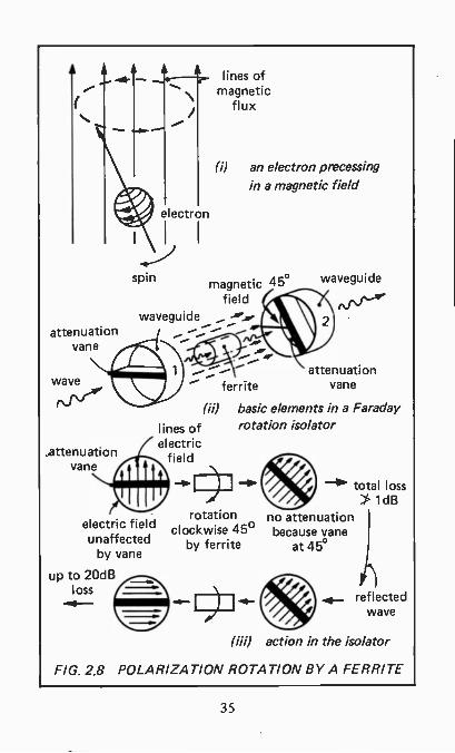
Looking further into electrons and their spins we fmd thatif a d.c. magnetic field is applied to an electron, the latterprecesses, in fact it acts like a gyroscope - see Figure 2.8(i).Precession is the slow movement of the axis of a spinningbody but we leave it at that for study of the peculiarities ofthe gyroscope might lead to many sleepless nights. Theelectron precesses at a rotational frequency which is depend-ent on the strength of the applied magnetic field. Interactionbetween an incoming microwave and the ferrite electrons ismaximum when the microwave frequency is at the precessionfrequency, known more technically as the gyromatic reson-ance frequency. We will not delve into this interaction, it issufficient here to note that wave polarization (Sect.1.4) canbe changed.

When a circularly polarized wave meets precessing electrons,it is found that there is interaction only when the waverotation is in the same direction as the electron spin. Now itcan be shown that linear polarization is made up of two equalcircular polarizations rotating in opposite directions. Hencelooking this way at a linearly polarized wave (e.g. TEM -Sect.1.4) when it is travelling through a ferrite in the samedirection as the static magnetic field, the two circularlypolarized waves representing it interact differently since oneaids precession of the spinning electrons whereas the otheropposes it. Accordingly their phase shifts are not equal andthe polarization is rotated. This rather sketchy explanationis illustrated in a practical way in the next two sections.

34

A

electron

lines ofmagnetic

flux

(i) an electron precessing

in a magnetic field

spin magnetic 45°field

waveguideattenuation

vane

wave

N

attenuationvane

electric fie dunaffected

by vane

up to 20dBloss

lines ofelectric

field

attenuation

waveguide

rdr-4r

ferrite vane

(ii) basic elements in a Faradayrotation isolator

rotationclockwise 45°

by ferrite

total loss> ldB

no attenuationbecause vane

at 45°

reflectedwave

(iii) action in the isolator

FIG. 2.8 POLARIZATION ROTATION BY A FERRITE

35

2.5.1 IsolatorsIt was Faraday himself who first saw the light (or did not asthe case may be). He discovered that a linearly polarized lightwave experienced rotation when transmitted through certainmaterials in a direction parallel to that of an applied magneticflux. Microwaves as we noted in Section 1.6, are not farremoved from light waves so we might reasonably expect thesame effect with microwaves and this is so. A sketch of thebasic elements of a Faraday rotation isolator is given in Figure2.8(H). In (iii) the rotation is further illustrated. When theelectric field lines of the microwave are at right angles to theattenuation vanes there is little attenuation but this steadilyincreases as the angle decreases from 90° down to 0°. Accord-ingly we see from (iii) that because the attenuation vane of thesecond waveguide is placed at 45° to that of waveguide 1, amicrowave travelling through 1 and 2 in that order sufferslittle attenuation. Conversely in the opposite direction theferrite rotates the wave polarization so that the electric linesrun parallel to the attenuation vane and the wave thereforeexperiences a high loss. Thus any reflections from the far -end

from Section 2.1.2 create undesirablestanding waves) are effectively removed.

There are many other configurations of isolators based onferrites. One in common use is a resonance type and here theresonance is of the precessing frequency. Interaction isstrong or negligible depending on the direction of propagationof the wave.

2.5.2 CirculatorsThe non -reciprocal phase -shifting characteristics of ferrites areagain used to advantage in circulators. Perhaps the mostfrequently used component is the 3 -port or Y circulator assketched in Figure 2.9. The device is effectively three isolatorsas described above built into one. Microwave power enteringport 1 is received at 2 only, that entering at 2 is received at 3only and that entering at 3 is received at 1. Typical uses areindicated on the diagram, i.e.:

(i) a transmitter at 1 feeds an antenna at 2. Power receivedfrom the antenna is fed to its receiver at 3;

36

transmitter(or amplifier)

ferrite

antenna(or load)

receiver (magnetic flux(or matched downwards

load) into paper)

FIG. 2.9 3-PORT CIRCULATOR

(ii) an amplifier output connected to 1 is coupled to theload at 2. Any reflected power from a mismatched loadre-enters the circulator at 2 and is dissipated in a loadconnected to 3.

Above are two examples only, circulators with more portsthan 3 are in use and as microwave requirements grow, ferntetechnology expands to satisfy them. Certainly ferrites havefound their place in satellite television in which the electro-magnetic wave transmitted down to us from the satellite maybe either vertically or horizontally polarized (Sect.! .4) and theunwanted polarization must be rejected to prevent interfer-ence (see Sect.5.3). The ferrite polarizes is mounted on thereceiving antenna (the "dish") and it can be remotely switchedto allow only the required polarization to pass to the receivingequipment. Practically all antennas are mounted in the openso the fact that the device is robust and is itself waterproof isan indication of its superiority over many alternative systems.

2.5.3 FiltersFerrites, especially of the yttrium iron garnet type are special-ly adaptable as band -stop and band-pass filters of narrowwidth. For this a single crystal of YIG is grown from a solution,

37

it then goes through a tumbling process with a fine abrasivepowder until a highly polished sphere is obtained. In use ther.f. magnetic field of the wave to be filtered is coupled to thecrystal by a loop at right angles to the d.c. magnetic fieldwhich controls the gyromagnetic (precession) resonancefrequency. At this frequency, because the YIG is a singlecrystal the energy of the r.f. wave becomes tightly coupledto the gyromagnetic resonance and is absorbed by it. Thisproduces a band -stop filter which is tunable over a widefrequency range by adjustment of the d.c. magnetic field.

A band-pass filter using the same type of YIG crystalsphere is slightly more complicated in that there are twoloops, one carrying the input r.f. wave, the second (output)close to it but at right angles. Because normally there is nocoupling between the input and output loops, the deviceattenuates the r.f. signal. However, at the gyromagneticresonance frequency (adjusted by the d.c. magnetic field)the two loops become coupled energy -wise within the crystaland the filter passes the wave but only over a narrow fre-quency band. An example of the use of a YIG band-passfilter is given in Section 4.1.

38

Chapter 3

MICROWAVE GENERATION AND PROCESSING

Although the transistor has rather indecently dismissed thevacuum tube (or electronic valve) in many electrcalics fields,it cannot do so yet for microwaves. Several different types ofvacuum tube still hold sway when large powers are required,especially at the highest frequencies. At present solid statedevices are mainly used at powers less than some 100 wattsfor frequencies up to 1 GHz, falling to a fraction of a watt at100 GHz. On the other hand a vacuum tube device such as aklystron can handle as much as 1000 kW although only overa narrow frequency range. Such powers of course are seldomrequired.

We might conveniently divide the whole range of generatorsand amplifiers as in the sections below.

3.1 Grid -Controlled Microwave TubesThis type assumes a vacuum chamber through which a streamof electrons flows. All rely on thermionic emission ofelectrons from a cathode, i.e. the emission of electrons fromthe surface of a material when it is heated. At room temper-ature few free electrons have sufficient energy for escapefrom the surface. They are then prevented from movingaway altogether by the space charge which they themselvescreate and by the fact that the atoms from which they haveescaped now exhibit a positive charge. Heating the materialprovides more electrons with the energy they need for escapebut accordingly the space charge increases. The restrainingeffect of the space charge is countered by surrounding thecathode by an anode which is charged positively. This positivecharge attracts electrons from the space charge and providedthat they have somewhere to go and can be replaced there is aflow of electrons from cathode to anode. Heat is provided bya heater element as sketched in Figure 3.1(i) which in factillustrates a conventional diode electronic valve.

A fine -wire mesh grid inserted between cathode and anodeas in (ii) enables us to control the electron stream, e.g. if a

39

evacuatedenvelope heating(metal or filament

glass)

cathode

cylindricalanode

(cut away toshow cathode)

cathode

connectingpins

(i) diode electronic valve

cathodesupport

heater

anode

grid

(ii) the addition of a grid forms a triode

yr-

anode (withcooling

arrangementsif required)

grid

gridmount

cathode

heater

(iii) electrode assembly of a planar triode

FIG. 3.1 GRID-CONTROLLED TUBES

40

negative potential exists on the grid, electrons are repelled butif the potential is positive electrons are encouraged to cross thegap. This arrangement constitutes the well-known triode valvewhich is basically of a tubular shape. When it comes to micro-waves, however, the tubular triode has its problems for nowthe relationship between electrode dimensions and wavelengthbegins to show. The later developed planar triodes are betterin this respect and the elements of such a device are shown in(iii) of the figure. They are especially useful in microwavegeneration where a crystal -controlled oscillator drives a multi-stage planar amplifier.

Summing up, the tubular and planar triodes function byspace charge control in which the density of an electroncurrent is varied. The performance tends to fall with fre-quency mainly because of the effects of electron transit timeand interelectrode capacitances. Tubes which suffer less fromthese disadvantages function by modulating the velocity ofthe electron stream rather than its density as discussed next.

3.2 Linear Beam Microwave TubesThese of a high -velocitypencil -like beam of electrons. Each tube requires a generatorof this type of beam, known as an electron gun. Such a deviceis not rare for it is from one of these that the picture on atelevision tube is ultimately derived. We might define anelectron gun as an assembly of electrodes for the productionof a concentrated beam of electrons moving at very highspeed (many millions of miles or kilometres per hour) andtherefore abounding with kinetic energy (k.e. = Y2mv2 wherem is the mass and v the velocity).

In the gun thermionic emission from a specially coatedcathode provides the supply of free electrons, they are thenaccelerated towards the positive field of an anode as sketchedin a simplified form in Figure 3.2. The cathode emittingsurface is of considerably greater area than the cross-sectionalarea of the beam since the current density required in thebeam is high. The focusing electrode is at cathode potential(or more negative) and serves to concentrate the beam asshown. The anode which is a metal plate with a circular holein the centre is at several kilovolts positive relative to the

41

vacuum

heater

focusingelectrode

root'

cathode

anode

concentratedstream ofelectrons

emittingsurface

highvoltagesupply

1

C3

FIG. 3.2 SIMPLIFIED ELECTRON GUN FOR LINEARBEAM TUBE

cathode. It is at earth potential so that output and input portsconnected to the device supplied by the gun may also be atearth potential. Careful shaping of all the electrodes producesa convergence of the electrons so that they pass through theanode as a high -velocity narrow beam. The electron beamcurrent (I) is given approximately by the relationship:

I = kV 3"2

where V is the anode -cathode voltage and k is a constant forthe particular electrode structure.

Needless to say, practical guns are more complex than thatshown in the figure and many variations are used dependingon the particular device for which the gun is designed.

42

The beam is useless unless it can be modified or modulatedin some way. This can be done based on the fact that eachelectron in the beam possesses kinetic energy because of itsmotion and if it enters an accelerating (positive) field it gainsenergy from the field and its velocity therefore increases. Onthe other hand, if it enters a retarding field the electrongives up energy to the field and its velocity decreases (here itis not essential for us to get involved with the minute correc-tions arising from Einstein and his relativity theory). Thus aradio frequency (r.f.) signal can be applied to an electron beamto alternately speed up and then slow down the passingelectrons. This is appropriately known as velocity modulation.The practical outcome is the basis of operation of theklystron, travelling -wave tube and backward -wave oscillator.

3.2.1 KlystronKlystrons come in all shapes and sizes, from the smallestsome 10 cm long, to a large one of length about 2 metres.They can be used as microwave oscillators or perhaps morelikely as amplifiers. The simplest klystron is a two cavitydevice (Sect.2.1.4), meaning that two resonant cavities arerequired, one to velocity modulate an electron beam, theother as the output system. These are known as buncherand catcher as shown in Figure 3.3. Between the two cavitiesis a length of tunnel known as the drift space or drift tube.Operation of the klystron follows from the electron gun andbasic idea of velocity modulation given in the precedingsection.

At one end of the evacuated tube is the electron gun, itsbeam passing first through the grids of the buncher cavity.The space between the grids is known as the interaction spaceand electrons passing through have their velocities changedaccording to the instantaneous r.f. potential existing acrossthe cavity. As the electrons leave the interaction space there-fore, some are travelling faster, some more slowly while othersare unaffected. They are now traversing the drift space inwhich slowed electrons are overtaken by the faster ones hencecreating bunches of electrons of density according to themagnitude of the input r.f. signal when the electrons werepassing through the buncher.

43

4 -

inpu

t

inte

ract

ion

spac

e

outp

utbu

nche

rca

tche

rca

vity

cavi

ty

drift

spac

e

elec

tron

reso

nant

elec

tron

gun

cavi

tybu

nch

grid

s

FIG

. 3.3

TW

O-C

AV

ITY

KLY

ST

RO

N A

MP

LIF

IER

evac

uate

dm

etal

vess

elco

llect

or

The catcher cavity is tuned to the same frequency as thebuncher. It is located along the tube at the point where theelectron bunching is maximum. Consider the two grids of thecavity, labelled g1 and g2 in the figure. If for example, due toan alternating field across the cavity g1 is positive to g2 ,then the bunches of electrons passing through will be slowed,hence as we have seen above, they deliver energy to the fieldwhich accordingly increases. In fact the phase relationship ofthe r.f. oscillation in the cavity relative to the arriving electronbunches adjusts so that the bunches are retarded because theoscillation amplitude cannot build up unless energy is extrac-ted from the beam. The power output is related to thedifference in average kinetic energy of the electrons as theypass from g1 to g2 . Following the catcher cavity is the collec-tor, simply a positive anode which removes the beam.

This is how a klystron amplifies: by arranging feedbackfrom the output cavity to the input cavity in correct ampli-tude and phase the device becomes a microwave oscillator.Alternatively a special design of tube known as a reflex klystronmay be used as a low power oscillator. This has only onecavity which serves as both buncher and catcher. The velocitymodulated beam is returned to the cavity by a reflectorelectrode.

When high power is required, a klystron may have morethan two resonant cavities, generally four but possibly more.Klystrons are sometimes used in telecommunications satellitesbut because as amplifiers they have a rather restricted band-width, travelling -wave tubes (see next section) are generallypreferred.

3.2.2 Travelling -Wave TubeThis type differs from the klystron in that the r.f. input wavetravels with the electron beam over almost its whole lengthand thereby is enabled to interact with it continuously insteadof only in a short (buncher) cavity. As might be expected,therefore, as amplifiers they are capable of higher gain andbecause no resonant cavities are involved, considerably greaterbandwidth is available.

Amplification by a travelling -wave tube (t.w.t.) arises fromvelocity modulation of an electron beam (Sect.3.2) by the r.f.

45

CN

CN

elec

tron

gun

evac

uate

dtu

beel

ectr

onbe

am

4 I

(ff

1

ffg-

c=fy

-e

atte

nuat

orhe

lixco

llect

or

inpu

tt

alba

sic

cons

truc

tion

axia

l com

pone

ntof

r.f.

fiel

d1.

slow

-wav

e st

ruct

ure

alon

g sl

ow-w

ave

''' --

.,..

.*-

.....

, ..4

.- ..

..-, -

01i-

...,:

stru

ctur

e \

.A.:,

...II

.- -

- ...

.Z. ,

.-1-

.* -

- ...

...'

\I.

><

-4.

-

outp

ut

Ns,

41-

/ /\

ail

ampl

ifica

tion

"1"-

elec

tron

sel

ectr

ons

acce

lera

ted

dece

lera

ted

-.4-

5.

- -ac

cele

rate

dw

ithbu

nchi

ng7

.t.,7

7r,p

r!..7

.7.

:77

r.7.

:*7.

7r:7

.,7.

elec

tron

beam

5)(

N"7

/ \-*

" //

\

elec

tron

-0.

elec

tron

leflo

wbu

nch

FIG

. 3.4

TR

AV

ELL

ING

-WA

VE

TU

BE

bunc

hde

cele

rate

dth

eref

ore

give

s up

ener

gy to

r.f.

field

input wave which is followed by electron deceleration to passenergy back to the wave. A sketch of the basic arrangement isgiven in Figure 3.4(i). An electron gun (Sect.3.2 again) pro-vides a narrow beam of electrons travelling lengthwise throughthe tube to a collector at the end remote from the gun. Ametal helix surrounds the beam as shown. This helix carriesthe input r.f. and although the wave travels around the helixwire at a speed approaching that of light, its velocity along thetube axis is considerably slower depending on the pitch andangle of the helix. In fact the helix is known as the slow -wavestructure. It is essential that the axial velocity is approximate-ly equal to that of the electron beam and when this is so thereis interaction between the beam and the r.f. wave.

The electron stream has a tendency to spread out due tothe mutual repulsion between the electrons. To maintainthem in a straight line an external longitudinal magnetic fieldis applied to repel the wanderers back into the stream; thefield is usually provided by a permanent magnet but a coil mayalso be used (not shown in the figure).

Needless to say the action is quite complex but we can getsome idea of how it all happens from Figure 3.4(ii), remem-bering that although the r.f. wave travels around the helix,it has an axial component which can react with the beamelectrons. In the drawing this component and the electronbeam are shown separated for clarity, the beam travels slightlyfaster. Electrons in the beam are alternately accelerated anddecelerated, i.e. they are velocity modulated, therefore creat-ing bunches. As a bunch progresses further along it is deceler-ated and so gives up energy to the field, resulting in an inducedr.f. current in the helix. Provided that this is in the correctphase, the r.f. signal is increased and is now able to produce adenser electric charge in the beam (bunch). The effect iscumulative and the wave builds up until the average velocityof the electrons in the beam is reduced to that of the travellingfield. As an amplifier the tube gain varies directly as theeffective length of the slow -wave structure. Power gains of60 dB are common.

We may be surprised to see of all things an attenuator in thecentre of the slow -wave structure. It is a device which allowsthe electron beam with its bunches to travel through unopposed

47

whereas the r.f. wave is reduced to almost zero. The techniqueprevents unwanted waves reflected from input mismatchesfrom being propagated to the tube input and therefore causinginstability. The amplified signal is removed from the helix bythe output coupling. Note that the energy employed inamplifying the r.f. signal is provided entirely by the electronbeam which can be looked upon as a d.c. source.

Alternative slow -wave structures may be employed or evena series of cavities, the basic method of operation however isthe same. Travelling -wave tubes are extensively used asamplifiers in television broadcasting (both terrestrial andsatellite), in microwave communication systems and in radarand military weapon systems.

3.2.3 Backward -Wave OscillatorTo have successfully coped with the operation of the travelling -wave tube (t.w.t.) may in fact make things a little difficultwhen trying to get to grips with the backward-wave oscillator.It seems to be a t.w.t. all over again yet the direction of energyflow in the slow -wave structure is in the opposite direction tothat of the electrons in the beam. Figure 3.4(i) applies exceptthat there is no attenuator, the electron beam has a hollowcross-section, the slow -wave structure consists of a flat metaltape and there is a single output coupling only at the electrongun end.

Visualizing the interaction process is not exactly child'splay and the unadorned statement that the phase and groupvelocities of the r.f. circuit are 180° apart may be of littlehelp. Nevertheless, from this it follows that the direction ofenergy flow (the group velocity) is directly opposite to thedirection of electron motion. This shows that a wave ispropagated backwards. We can look a little more closely intothe process by considering a section of the slow-wave structureas in Figure 3.5. As with other oscillators, noise voltages (e.g.from the electron beam) induced in the slow-wave structureare sufficient to start a build-up of oscillations.

In the figure the electric field existing across adjacent helixturns is shown. As mentioned in Section 2.3.1, an electricfield cannot exist parallel and close to a conducting surface,accordingly under each turn of the helix the field is zero with

48

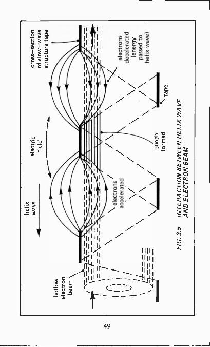
hollo

wel

ectr

onbe

am

\

helix

wav

eel

ectr

icfie

ldcr

oss-

sect

ion

of s

low

-wav

est

ruct

ure

tape

111.

1

esm

°°11

°

Nt4

irpiO

goa0

1el

ectr

ons

a(ac

cele

rate

ds

/\

\em

m/

bunc

hfo

rmed

\ tape

FIG

. 3.5

INT

ER

AC

TIO

N B

ET

WE

EN

HE

LIX

WA

VE

AN

D E

LEC

TR

ON

BE

AM

elec

tron

sde

cele

rate

d(e

nerg

ypa

ssed

tohe

lix w

ave)

a maximum midway between the turns as shown. As with thet.w.t. the electrons in the beam are alternately accelerated anddecelerated. In a way this transfer of energy can be lookedupon as a feedback system between mid -points of adjacenthelix gaps and provided that phase relationships are correctlymaintained by adjustment of beam velocity, the generatedwave flows backwards and the system can be made to oscil-late. It is also necessary to ensure that each group of electronsis affected by an electric field of the same phase as it passesalong the slow -wave structure so that one group is continuallyaccelerated while the following group is decelerated. Thebackward helix wave builds up and flows in a directionopposite to that of the electron beam and is extracted througha coupling at the gun end of the tube.

Low -power backward -wave oscillators are those havingpower outputs ranging from 10 to about 100 mW with operat-ing frequencies extending over the whole of the microwaveband. Power backward -wave oscillators are more likely toemploy mutually coupled cavities instead of a metal tapehelix. Output powers range from about 1 mW to 40 W overa frequency range from some 20 to 300 GHz.

3.3 Crossed -Field Microwave DevicesAs its name suggests, a linear beam tube is based on anundeviating stream of electrons. A magnetic field is involvedbut this is merely to keep the beam in order. The crossed -field type also employs a magnetic field but its purpose isnow more fundamental, not to keep the electrons from stray-ing from a straight and narrow path but in fact to encouragethem to do so. Perhaps we should first refresh our memorieson what a field can do to an electron.

In Figure 3.6(i) suppose an electron of charge e is travellingalong the line from A to B at a velocity v through the twofields at right angles, one electric, the other magnetic (thecrossed fields) as illustrated. The magnetic field is horizontal,has a flux density B and is in the direction shown by thearrows on the flux lines. The electric field is vertical and theflux lines have been omitted because shown conventionallythey would be arrowed downwards which may be confusing.

50

D4-_...,

4-

4.it ..'"--."

4 . , -*"C 4. ' -...-

F

I

ir EB 1 90°...._h magnetic

(charge = e)electron I v ,,,-(2 flux lines

\ \ X\\ \I \ \ R.A '<.0 . . . .

R \\ \ \ \ \ ... >\ \ R \ \ I

......-F\ F ...--\ M \5' '

10.", ....'(i) forces on an electron

travelling in crossed fields Emagnetic fluxdownwardsinto paper

Anode)

#Jr'

/ ba 1

...-- 4' - --c

-.. ...--

FE

I /It, N /v ir V -

4

FM

cathode

-$1

(ii) some electron paths

O

FIG. 3.6 ELECTRONS IN CROSSED FIELDS

51

It is sufficient to postulate that along the line CD is a positivecharge. Using a right-hand rule (i.e. with fingers extended asoriginally suggested by Fleming - this is electron flow, notconventional current), there is a force FM acting downwardson the electron due to the magnetic field such that with0 =90° :

FM = evB

and we note that the force varies with the velocity of theelectron. If 0 is other than 90° then the formula for FMbecomes evB sin 9. In the opposite direction the electric fieldexerts a force FE upwards on the electron such that FE = eEwhere E is the electric field strength.

If we wish our electron to continue its journey undisturbedthen:

hence:eE = evB

v = E/B.

When this condition does not apply the electron is deflec-ted from its straight path. From this we now may begin tosee the basis on which a crossed -field device works. Theelectric field is at microwave frequency and the magneticfield is provided (usually) by a permanent magnet. Thecombination of the electric and magnetic fields is used tomake electrons deviate in many curvaceous ways. Here isjust one simple example, illustrated by Figure 3.600. In thiscase we must imagine the magnetic flux as being downwardsinto the paper. The line CD in (i) of the figure is now ananode and AB is a cathode. With zero magnetic field theelectrons follow the path (a). As the magnetic field isincreased, electrons move in a curved path (b). A furtherincrease in the field prevents electrons from reaching theanode and they return to the cathode. We will see that manyother gyrations are possible which may seem pointless untilwe recall that accelerating electrons take energy on boardwhereas when decelerating, they give it up.

52

3.3.1 MagnetronThis is perhaps the best known of all crossed -field devices,mainly because of its early development for use in radarsystems. It has now entered the home as the power behind(or in) the microwave cooker. Many types of magnetronexist, one which is in common use and lends itself to(moderately) simple explanation is the 8 -cavity magnetronoscillator as illustrated in part in Figure 3.7. The anode is acircular block of metal (usually copper) in which are cut 8holes and slots as shown in (i). The holes are in fact cavitiesall resonating at the same frequency and to one is coupled awaveguide as the output port. The cathode is fixed in thecentre of the block, leaving an interaction cavity between itand the inner surface of the anode as shown in (ii). A perman-ent magnet is usually employed to create the magnetic field,the "lines" of which are downwards into the paper in thisparticular drawing.

Some random effect sets up weak oscillations in the cavityresonators and these give rise to electric fields crossing theslots and extending into the interaction space as shown in thesketch for a particular instant. In this arrangement alternateslots support fields in opposite directions, the magnetron isthen said to operate in the v -mode.

Magnetron operation is highly complex so the simplifiedexplanation which follows can only serve to furnish anappreciation of the ingenuity on which it is founded. Wecannot expect to understand it in detail; even the mechanicaland electronic methods adopted for tuning the cavity structurewould require many chapters on their own.

Let us consider the path of an electron liberated from thecathode. From Section 3.3 it clearly does not move in astraight line directly to the positive anode because the (d.c.)magnetic flux causes it to curve to the right (the right-handrule again). Our electron enters the r.f. electric field of cavity1 which is in the direction shown. The direction is such as toretard the electron which therefore transfers energy to thefield. The electron slows towards point a but is again acceler-ated by the d.c. field. Now it comes under the influence ofthe r.f. field of cavity 2 but note that while the electron hastravelled to a, the r.f. field has changed by 180° Or radians)

53

hole(resonantcavity)

r.f. electricfield

\\

1

magneticflux

cathode

interactioncavity

path ofelectron

(i)

Nslot

part ofcopperanode

single resonant cavityin anode structure

resonantcavities

(ii) part of 8-cavity magnetron

FIG. 3.7 MAGNETRON

54

and is therefore in the opposite direction to that shown in (ii)of the figure. The process which we observed under cavity 1is now repeated under cavity 2 and electron energy is againtransferred to the field as the electron moves on to b. Atcavity 3 the r.f. field has passed through 360° so is as shownand the same interaction continues. As energy is given up,gradually the electron moves closer to the anode and is finallyseized by it, although this may be after many orbits aroundthe cathode. Other electrons may not be so useful as agentsin the energy transfer process. Some are soon collected bythe anode, some revert to the cathode. Those which findthemselves in an unfavourable position for energy provisionbecause they are in the alternate phase of the r.f. field absorbenergy are therefore accelerated and move back towards thecathode. Nevertheless, the whole process can be considered asa cloud of electrons rotating round the cathode in synchron-ism with the r.f. field and delivering energy to it.

Commercial magnetrons are available with mean outputpowers of between 10 and 100 kW at 1 GHz but down to afraction of 1 kW at 100 GHz. Peak output powers howevermay be several hundred times greater.

3.3.2 Crossed -Field AmplifiersOf the many varieties of crossed -field amplifier which exist,one which is commonly used is in fact quite similar to themagnetron. Actually the crossed -field amplifier is a logicalextension of the magnetron (an oscillator) into an amplifier.As an amplifier there must of course be both input andoutput ports. Figure 3.8 is an imaginary crossed -fieldamplifier drawn to show the main basic operating features,practical devices may look very different.

Conversion of an 8 -cavity magnetron into a crossed -fieldamplifier requires special conducting straps connected asshown to reduce the build-up of unwanted modes (Sect.2.3.2).The straps are not simply electrical connections (the anodeblock is usually solid copper anyway) but are recessed intothe anode structure as shown in the cross-sectional view. Fora n -mode device as described in the preceding section, thestraps join segments which are at the same r.f. voltage asshown. Each strap has inductance and also forms a capacitance

55

r.f. input

energyflow

resonantcavity

straps

strapconnected

anode

cross-sectionalview

r.f. output

anode

interactionspace

//strap running

betweensegmentson eachside (not

connected)

FIG. 3.8 CROSSED-FIELD AMPLIFIER

56

coupled to the segment in which it is recessed. The capaci-tance is effectively in parallel with the resonator hence reducesslightly the resonance frequency of the it -mode. However,for other lower modes it can be shown that there is an increasein the resonance frequency and so the separation between thewanted and unwanted modes is increased.

Note the increased interaction space (the drift space)between the input and output ports. Its purpose is to mini-mize feedback from output to input which would cause thedevice to fail as an amplifier because of oscillation. In passingthrough this space electron bunches in the rotating cloud ofelectrons travelling past the output port have time to dispersebefore they reach the input port.

Peak output power levels of the various crossed -fieldamplifiers available are surprisingly high. They vary over awide range from between 100 kW and 5 MW at 1 GHz to100 kW at 16 GHz. Gain of a single unit is of the order of15 dB.

3.4 Semiconductor DevicesNaturally the development of semiconductor devices for use atmicrowave frequencies has made rapid strides. The maindifficulty is perhaps obvious, semiconductor junctions havecapacitance which at the higher frequencies is ruinous.Accordingly the earliest attempts to enlist semiconductortechnology revolved around the point -contact diode whichuses a metal whisker in contact with a semiconducting materialand therefore has comparatively low junction capacitance.More recently special semiconductor components have beendeveloped for microwaves. This cannot be an exhaustivesurvey of the whole field but a few examples may be usefulhere to demonstrate the underlying techniques.

Transistors we recall are broadly divided into two types:(i) bipolar which depend for their action on the flow of bothmajority and minority carriers with their terminals labelledemitter, base and collector; and (ii) field-effect, also known asunipolar, and which depend on the flow of majority carriersonly. Their terminals are labelled source, gate and drain. Wewill see that much development for microwave use has centred

57

around special constructions of the field-effect transistor(f.e.t.).

3.4.1 DiodesCertain diodes are capable of amplification or sustaining oscil-lation if they have a negative resistance characteristic over thefrequency range required. This needs some explanation sofirst we refresh our memories with the basic p -n junctioncurrent/voltage characteristic extending into the avalanchebreakdown region as shown in Figure 3.9(i). When the d.c.voltage (Vdc) applied exceeds the breakdown voltage,avalanche multiplication generates an additional supply ofelectrons and holes and these flow in the depletion regionwhich increases in width on the n -side of the junction accord-ing to the magnitude of the voltage applied.

Consider a diode maintained in the avalanche condition bya voltage Vdc and with an r.f. voltage v sin wt acting as shownin (ii) of the figure. The supply of charge carriers generatedwill vary as the net voltage applied but not in phase with itbecause a negative resistance condition exists where the

the voltage increases. In effect the maxi-mum rate of supply of charge carriers occurs at over 90° afterthe applied voltage maximum. Following this the electronsdrift across the depletion region and while doing so theyconstitute a current in the external resonant circuit. Thus thetotal delay of avalanche plus drift time ensures that thecurrent is flowing and therefore energy is being delivered tothe external circuit even while the applied r.f. voltage is in itsnegative half -cycle - see (ii) of the figure (don't be misled bythe standard use of the term "drift", the total delay time at10 GHz might be a mere 40 picoseconds). Most of the energyis provided by the circuit power supply.

Three diodes currently in use as microwave amplifiersand/or oscillators which are worthy of mention here are:

1. tunnel diode: this type is constructed with heavy doping onboth sides of the junction resulting in a very narrow poten-tial barrier. Accordingly charge carriers can "tunnel" acrossthe depletion layer even when no potential difference isapplied. Put in other words, electrons which normally

58

(i)ju

nctio

n di

ode

char

acte

ristic

aval

anch

epo

int

forw

ard

reve

rse

rate

rate

of

aval

anch

evo

ltage

app

lied

gene

ratio

ncu

rren

tto

dio

deof

cha

rge

(Vdc

+ v

sin

wt)

carr

iers

..--.

.....

- ...

,.\

/s.

curr

ent

/.

1/ f

low

//

\11

\/\

//tim

e, t

--..

\//

....

,...

.-

(ii)

even

ts in

a c

ycle

in a

dio

de u

nder

ava

lanc

he b

reak

dow

n

FIG

. 3.9

AV

ALA

NC

HE

DIO

DE

S

Vdc

would not have sufficient kinetic energy for overcoming thepotential barrier, now have no need of it, the energies theypossess as valence electrons are sufficient for them to leavehome and jump the barrier as conduction electrons. Withforward bias a negative resistance region develops which isvoltage controlled. Tunnel diodes are sufficiently fastacting to be useful for microwave amplification (but atvery low power) and for microwave oscillators.

2. IMPATT diode: the acronym IMPATT is derived fromIMPact ionization Avalanche Transit Time which is intend-ed to define how the device works. Its main use is in thegeneration of microwave power and operation is basedmainly on the principles outlined above, i.e. as a diodereverse -biased into avalanche breakdown; typically Vdcis around 100 V. In use the diode is mounted in a resonantcavity with impedance matching. Typically an IMPATTamplifier might have a maximum power output of about100 W at 10 GHz with a gain of 10 - 12 dB. Efficienciesare fairly low at 10 - 20%. As an oscillator output powersapproaching 100 W are possible at up to 10 GHz but gener-ally lower than this at higher frequencies.

3. Transferred Electron (Gunn) Device: in this the specialeffect arises in a single semiconductor material (i.e. there isno p -n junction) usually of gallium arsenide or indiumphosphide. The basic mechanism is different from that in"normal" diodes and it was first reported by J. B. Gunn in1963 hence it is also known as a Gunn device or Gunndiode.

Gunn discovered that a d.c. voltage applied to a bar of n -type gallium arsenide or indium phosphide at first produced acurrent increasing linearly with the voltage but above a certainthreshold voltage the current oscillated. The threshold voltageis around 300 kV/m which seems exceedingly high until werealize that practical devices may have an effective length assmall as 0.1 mm, hence requiring a voltage of about 30 up-wards. Gunn found that the current oscillations were closelyrelated to the transit time of the electrons along the slice. As

60

an example, for gallium arsenide the maximum election driftvelocity (v) is about 105 m/s so for a 0..1 mm length (1) theoscillation period (t) ^ //v = 10-9 seconds and the frequency= lit, i.e. about 1 GHz. The necessary negative resistancefeature is shown by the current density/electric field character-istic shown in Figure 3.10(i) which we can interpret for agiven specimen as a current/voltage characteristic, the negativeresistance is evident above about V = 300 kV/m.

The basic mechanism is complex and is usually explained interms of electron energy levels but it may be possible tovisualize it in a rather simplified fashion through considerationof the space charge (Sect.3.1). Picture a small slice of galliumarsenide connected to a d.c. voltage supply which exceeds thethreshold voltage. At the negative contact (the cathode) aspace charge builds up with a consequent increase in itselectric field. As it does so the voltage across it increaseshence the voltage across the remaining region towards thepositive contact (the anode) falls below the threshold value.The accumulation of space charge is known as a maturedomain. Now this is taking place as part of a moving electronstream and in a way we can imagine the domain as being sweptalong with the current increasing and then decreasing andfinally flowing out at the anode, hence the name transferredelectron device. The process continually repeats at microwavefrequency.

In the practical device the active region as shown in (ii) ofthe figure is an n -layer whereas the "contacts" are n -regions,highly doped for good conductivity (marked n.). Oscillatorsof this type may have continuous wave outputs of up to 1 Wat 10 GHz falling to around 100 mW at 40 GHz. Noise gener-ated is low compared with most other types of microwaveoscillators. Practical amplifiers may have gains of 10 - 30dB over the range 10 - 50 GHz, depending on the numberof stages.

Demodulation or detection is the process through whichinformation impressed on a carrier wave is regained. Foramplitude modulation systems the basis of most detectors isthe non-linear characteristic of a diode. For frequencymodulation systems (e.g. microwave telephony and satellite)the circuit is known as a frequency discriminator and is more

61

currentdensity

f

negativeresistance

0 300 600 900electric field, kV/m

(i) current density/electric field characteristic forgallium arsenide

metalcontact

contact layer(low resistance)

substrate(low -esistance)

metalcontact

(ii) typical construction

FIG. 3.10 TRANSFERRED ELECTRON DEVICE

62

complicated but is still likely to be based partly on diodes.Two suitable types of diode are mentioned below:

4. Schottky diodes: microwave p -n diodes are limited at thehigher frequencies because of the relatively long lifetimesof the minority carriers. Lifetime is the mean time intervalbetween generation and recombination of the chargecarriers and in the diode this means that it will not respondsufficiently quickly hence in a detector resulting in reducedefficiency. The Schottky diode relies for its rectifyingaction on a barrier formed at the junction between a metaland a semiconductor, e.g. aluminium or nickel -chromiumwith n -type silicon. With such a junction the current flowis mainly by majority carriers, hence minority carrier dif-fusion is small and less of an embarrassment at the highermicrowave frequencies. Special mesh constructions allowoperation up to about 40 GHz, with gallium arsenide it ispossible to exceed 100 GHz.

5. Backward diodes are similar to tunnel diodes (see 1) exceptthat the doping levels are slightly lower. The current/voltage characteristic is such that at low reverse bias(almost zero) the diode breaks down. In the forwarddirection at low voltages the characteristic is very non-linear and it is this which makes the diode suitable for useas a detector. Being a majority carrier device the diode hasa high speed of response and is usable up to at least 20GHz.

3.4.2 Bipolar TransistorsCompared with the semiconductor diode the additionalelectrode gives more control. Arranging for microwavepurposes mainly involves keeping reactances (mostly capaci-tive) and parasitic resistances as low as possible. Accordinglymicrowave bipolar transistors are manufactured using planartechnology and are of extremely small dimensions, e.g. withactive surfaces of less than one thousandth of a square milli-metre. Needless to say, except for power transistors thepower handling capacity of such a tiny device is small. One

63

advantage of the microwave bipolar transistor is its low cost.Operation of silicon types extends up to some 6 GHz for bothamplifiers and oscillators.

3.4.3 Field -Effect TransistorsThese as normally used have little more to offer than thebipolar. However, specially constructed field-effect transistors(f.e.t.'s) are capable of operation up to 100 GHz althoughuseful amplifier gains are limited to around 10 GHz. Thespecial construction results in the device being known as aMESFET which is an acronym derived from metal -semiconductor f.e.t. The simplicity of a MESFET can bejudged from the diagrammatic sketch of Figure 3.11. Theconstruction is similar to that of a conventional f.e.t exceptthat the p -n junction at the gate electrode is changed to ametal -semiconductor junction, in this case aluminium (Al) ton -type gallium arsenide (GaAs).

We need not delve too deeply into the significance ofFermi levels, it is sufficient here to say that this is the particu-lar level of energy for a material at or just below whichelectrons contribute most to the conductivity. The Fermilevel of gallium arsenide is greater than that of aluminium,accordingly there are more available free electrons in theGaAs. At the area of contact the Fermi levels must be equalhence the higher energy electrons of the GaAs flow into thealuminium so leaving a positive charge in the semiconductorand a negative charge in the metal at the junction. A junctionbarrier potential equal to the initial Fermi level differencearises and a depletion region is formed in the semiconductorowing to the loss of charge carriers.

If now a potential is applied between source and gate thecharge pattern is modified. The depth of the depletion regionmust also change since its volume depends on the junctionbarrier potential. Majority carrier flow (electrons) is fromsource to drain and since the depletion region restricts thechannel available for electron flow the drain current is simi-larly modified. Thus r.f. potentials applied to the gate appearamplified in the load. Note that since the d.c. potential alongthe bar rises positively from source to drain, the depletionlayer is not of constant depth but varies as suggested in the

64

Ji

r.f.

inpu

tso

urce

cont

act

depl

etio

nre

gion

alum

iniu

mga

te

junc

tion

drai

nco

ntac

t

/el

ectr

on(1

.n-

type

flow

((-0

chan

nel

GaA

s

sem

i-ins

ulat

ing

GaA

s su

bstr

ate

I

FIG

. 3.1

1C

ON

ST

RU

CT

ION

OF

A M

ES

FE

T

drai

n cu

rren

t(e

lect

rons

)

load

drawing.These devices can be made very small, hence electron

transit time is short. In addition, electron mobility in GaAs is3 to 4 times that in silicon. Electron transit time and electronmobility are key factors in determining the high frequencyresponse of a semiconductor device (or in fact, any device).When a high frequency wave initiates action (usually a flow ofelectrons) within a device, this must be completed as far aspossible before the wave polarity reverses. Election velocitythrough a semiconductor device increases with electronmobility as might be expected. High velocities (some 105m/s for GaAs) result in shorter transit times. GaAs is superiorto silicon in this respect hence the GaAs MESFET has betterperformance at microwave frequencies compared with thenormal silicon f.e.t.

These MESFET's being basically transistors are usable in avariety of applications, especially in low -noise integratedcircuit (IC) amplifiers and oscillators. For IC's the generalclassification MMIC (monolithic microwave integrated circuit)may be used. Power MESFET's can be connected in Class Bfor higher efficiencies. Their low cost and good performancemake them replacements for other devices such as diodes andeven the travelling -wave tube.

Research into GaAs microwave integrated circuits (GaAsMMIC's) continues apace and complete circuits on a chip areavailable working at frequencies in excess of 20 GHz. Thepacking density can be very high, for example a 6 GHz chipcontaining microwave filters, amplifiers, output amplifier androuting switches (some 40 f.e.t.'s + 150 components) can berealized on a chip of area less than 10 mm2. Before MMIC'scame along "breadboard" designing allowed the insertion ofadjustable tuners, capacitors, potentiometers, etc., so thatcircuit action could be varied to maximize performance.Naturally MMIC's are not likely to permit such arrangements,hence their design is more complex and computer aid is usual-ly required. In addition, it perhaps goes without saying thatowing to the extremely small size of microwave devices,circuit analysis and testing present many difficulties.

66

3.4.4 Parametric Amplifiers"Parametric" implies that at least one parameter in the systemis non-linear or varies with time. On this basis microwaveamplifiers are designed around the variation in capacitance of avaractor diode. This small, specially constructed semiconduc-tor diode is located in a suitable microwave resonant cavityand the energy source for amplification is derived from a highfrequency wave (the pump frequency) instead of from a d.c.supply as with most other systems. We revise our understand-ing of the varactor diode first. The varactor diode (or justplain varactor - from variable reactor) is well known for itsuse as an electronically controlled tuning capacitor in a radioor television receiver. Its capacitance is small but this is not anembarrassment in microwave applications.

In any reverse -biased semiconductor diode the depletionlayer contains very few charge carriers so the layer has a highresistance (e.g. > 10 MS2) and is effectively a dielectricbetween two conducting plates, the n- and p -type regions. Thevaractor therefore acts as a parallel plate capacitor. What isimportant is that the width of the depletion layer varies withthe applied reverse voltage, hence the device can be used as avoltage controlled capacitor, the capacitance falling as thereverse voltage is increased. At microwave frequencies only apicofarad or so may be required with a variation perhaps inexcess of half a picofarad for a 4 - 6 V change; there is awide variation however, so much depends on the method offabrication. Certainly gallium arsenide is preferred as thesemiconductor for it has a higher frequency response com-pared with silicon because of its higher electron mobility. Italso has a lower series resistance (i.e. the resistance throughthe semiconducting materials to the depletion layer) whichincreases the efficiency since very approximately:

1

Q27rfrsC

where f is the frequency of operation, r3 is the series resistanceand C the capacitance.

The parametric amplifier was developed in the USA and itcunningly exploits the fact that with any variable capacitor

67

inductancecapacitance of resonantof varactor vt cavity

C -r1(i) parallel LC circuit

varactorcapacitance

normal \-cu

I I I/7Cas

I /I

minto

11t2t3

V \ I

pump voltageapplied tovaractor

t41 t5 time

I #'-. gain inI

/ voltage

time

voltageacross

LC circuit

(ii) showing how V increases when the varactorcapacitance falls

FIG. 3.12 PARAMETRIC AMPLIFICATION

68

(such as a varactor), if at any instant the capacitance changes,then the voltage (V) across it must also change since nothinghas happened to the charge (q) and V = q/C.

The explanation which follows is simplified so that thebasic technology can be revealed. Practical parametric ampli-fiers need several additional components to make it all happen.Consider a parallel tuned circuit as representing the capaci-tance of a varactor diode within a microwave resonant cavityas shown in Figure 3.12(i). A frequency at twice that of theoutput is applied to the varactor, this is the pump frequency.Suppose the varactor capacitance is "normal" at times to , t2,t4 , etc., but falls to a certain minimum at t1, t3, t5, etc. Fromto to ti the voltage, V across the LC circuit rises but note thatby t1 the varactor capacitance has decreased, hence fromV = q/C, V rises. The signal frequency therefore experiencesa voltage gain, the energy for this being supplied by the pumpfrequency. Note that the upper pair of curves in (ii) of thefigure assume a linear relationship between reverse voltageapplied to a varactor and the junction capacitance. This iscertainly not the case but the assumption is made for clarity.

At t2 the pump voltage is minimum so that the capacitancerestores to its normal value and this is exactly when the signalvoltage passes through zero, hence it is unaffected. At t3 thepump voltage is maximum with the capacitance falling, henceV gains another increase as shown. There is no change at t4but this is followed by another increase at t5. It is evidentthat the pump voltage must be applied in the correct phaseotherwise such gains will not be realized and the LC circuitoscillation will be damped.

Practical circuits involve more stages than the aboveexplanation would seem to indicate, especially in that theinput and amplified output signals must be kept separateand for this a circulator (Sect.2.5) is employed. For basicamplifiers we have seen that the capacitance changes mustoccur at exactly the right times so to ensure this a secondresonant (idler) circuit may be employed. However, in spiteof what has been said, there are other systems in which thepump frequency differs from twice the signal frequency.

There is a maximum frequency of operation, it is greatlyaffected by the varactor series resistance (rs). The formula

69

is simply:1

2Irrs Cb

where ft is the frequency of cut-off and Cb the capacitance atbreakdown. We compare two practical diodes, both havingCb = 0.11 pF but A has rs = 48 n whereas for B, rs = 5.3 fl.Then for A, fc = 30 GHz but for B, ft = 273 GHz showingthat for a high signal frequency the varactor must be con-structed with rs as low as possible.

The parametric amplifier is noted for its low noise per-formance, it is even better if the device is cooled. A 20 dBgain amplifier might have a bandwidth of around 2% of theoperating frequency, wider bandwidths can be achieved withlower gains.

3.5 MixersCommunication by microwave radio invariably employs somesort of frequency -changing or conversion, e.g. a complex wavecarried by a frequency f1 may be centred on a new frequencyf2 with none of the information contained in f1 changed inany way. Reasonably the device or circuit employed is knownas a frequency changer but because it involves the mixing oftwo frequencies it is perhaps more commonly known as amixer. This term is not fully descriptive of the action formerely adding two waves together does not produce the effectrequired unless they are mixed non -linearly. To be moreprecise, mixing is defined as the conversion of a signal of lowpower from one frequency to another by combining it with asignal at higher power in a non-linear device. The higherpowered signal (fo) is generated by a local oscillator.

Mixing produces a whole host of sum and differencefrequencies but the one usually picked out is the straight-forward difference between the two being mixed, i.e.:

f2 = fo -Microwave semiconductor diodes (Sect.3.4.1) are well

suited for microwave mixing and a rectifier bridge circuit in

70

common use is that of the double -balanced mixer which wellsuppresses in the output both fo and fi and certain harmonics,thereby reducing the complexity of subsequent filtering. Themain elements of such a circuit are shown in Figure 3.13.

Baluns are employed at the inputs of fo and f1. The term is anacronym from balanced -to -unbalanced (or vice versa), indicat-ing a type of transformer used to couple a balanced impedance(as is the double -balanced mixer), to an unbalanced inputsuch as a coaxial cable. As an example, a simple balun mayconsist of a short-circuited quarter -wave section of a trans-mission line attached to the outer braiding of the cable. Thisis arranged to present a very high impedance (Sect.2.1.3) toany wave arriving via the cable outer conductor, in otherwords, effectively disconnecting its coupling to earth.

71

Very briefly, it can be seen from Figure 3.13 that the largevoltage of fo alternately switches D1 and D2 then D3 and D4"on" and "off" thereby "chopping" fl at the frequency fo.The circuit also shows clearly that neither fo nor f1 is trans-mitted to the output terminals (f2).

Mixing is part of the superheterodyne principle which isthe backbone of radio receivers generally, f1 is the incomingsignal frequency and the mixer output (which we havedesignated h) is known as the intermediate frequency (seealso Sect.4.1). Although the above explanation is centred onsuitable microwave diodes, other types of mixers are worthyof mention. Certain transistors can be used with mixing takingplace across the base -emitter junction so that h is subsequent-ly amplified by transistor action. Compared with diodeshowever, the transistor is likely to have an inferior noiseperformance. Of interest too is the parametric converter,similar to the parametric amplifier (Sect.3.4.4) but adapted forfrequency conversion. Varactor diodes are semiconductordiodes which behave as voltage -dependent capacitors and thesemay be employed as with the amplifier with their capacitancesvaried on a time basis by the local oscillator (the pump).

72

Chapter 4

MEASUREMENT

Little can be achieved in research and development withoutmeasurement for we then neither know how things are norwhat we have done. Most of the measurement techniquesnowadays employed have been specially developed for micro-waves because of the limitations of standard (lower frequency)equipment. A particular example of this is given by thecathode-ray oscilloscope (c.r.o.) which is unable to displaymicrowave voltage waveforms above a few GHz. In thissection we look at just three types of measurement whichare essential for most systems. It must be emphasized thatwhat follows is far from complete, we are only scratching thesurface of measurement, the intention is mainly to illustratethe differences between "standard" measurement practicesand those used for microwaves.

4.1 FrequencyThis is probably the most fundamental parameter needed fordescription of a wave. As mentioned above the standard c.r.o.cannot cope but fortunately recourse may be made to severalother methods, for example cavity resonators (Sect.2.1.4)and transmission line resonators (Sect.2.1.2). These resonateat certain known frequencies which can be adjusted byplungers and are capable of good accuracy.

More modern is a system based on the digital counter, suchan instrument normally has microprocessor control. Typicallya digital counter may employ a Schmitt trigger to convert anincoming continuous wave into a corresponding train of pulsesas shown in Figure 4.1(i). The counter section then counts therate of arrival of the pulses and displays the result. To bringthe input frequency down to a value at which the counter canoperate, the superheterodyne principle is employed as shownin Figure 4.1(h). For the benefit of some readers we perhapsfirst need to recall the superheterodyne technique which isthat when a local oscillator frequency (fosc) is mixed with a

73

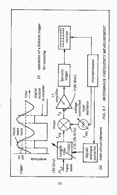
ontr

igge

rof

f

V 4-,

E cc

(10

GH

z)

inpu

tw

ave

form

- -

-

.

mix

er

time

digi

tal

outp

utto

cou

nter

i.f.

ampl

ifier

(i)op

erat

ion

of a

Sch

mitt

trig

ger

for

coun

ting

r\i

tuna

ble

sig

Sch

mitt

1111

0ME

NN

O

inpu

tfil

ter

trig

ger

coun

ter

wav

e/(

YIG

)(1

0.12

5 G

Hz)

volta

ge(1

25 M

Hz)

cont

rolle

dlo

cal

digi

tal/

osc

osci

llato

ran

alog

uem

icro

proc

esso

rco

nver

ter

(ii)

mai

n ci

rcu'

t ele

men

tsF

IG. 4

.1M

ICR

OW

AV

E F

RE

QU

EN

CY

ME

AS

UR

EM

EN

T

signal frequency (fsIG) in a non-linear device, sum and differ-ence frequencies (foss + fsiG) and (foss -fsiG) are generatedand one of these (usually the latter) is filtered off as theintermediate frequency (fIF) so that:

fiF = (fosc -fsiG)

for example as shown in the diagram in brackets, when a localoscillator frequency of 10.125 GHz is mixed with a signalfrequency of 10 GHz, the outcome is an intermediate fre-quency of 0.125 GHz (125 MHz).

The microprocessor adjusts the tunable band-pass filter(Sect.2.5.3) to select the wave to be measured while rejectingharmonics and other unwanted frequencies. The input wave-form and that of a local oscillator controlled by the micro-processor are mixed so that the intermediate frequency isgenerated as confirmed by the counter. The local oscillatoris voltage controlled (e.g. varactor tuned - Sect.3.4.4) so itsfrequency is known to the microprocessor from the magni-tude of the voltage which has to be applied. The micro-processor therefore is able to calculate and display the inputwave frequency on the counter. Clearly accurate calibrationof the local oscillator is essential and this is subsequentlymaintained by a crystal controlled reference oscillator (notshown). This is simply the basic system, many other refine-ments are built in when truly precise frequency measurementsare required.

It is worth noting that in frequency we have one parameterof a wave which, unless it meets deliberate frequency changingon its way, is not changed even minutely as it travels through asystem. This is more than can be said for most other para-meters such as voltage, current, power, attenuation, etc.

4.2 PowerAt frequencies lower than microwave we are used to measuringelectrical power in terms of voltage, current and resistance.We can appreciate that these quantities are not easily measur-able for microwaves when we consider not only the frequenciesencountered but also the fact that transmission is often by

75

waveguide where "terminals" tend to lose their meaning. Atmicrowave frequencies therefore power is frequently measuredvia the change in resistance of a thermally sensitive element.

4.2.1 BarrettersA bolometer is defined as an electrical instrument for measur-ing heat radiation, hence in microwave engineering the term isgenerally used to describe a resistive, temperature -sensitiveelement which undergoes a resistance change when it absorbselectromagnetic radiation. One type of microwave bolometeris the barretter which is especially useful for the measurementof low and medium powers. This in essence may be a plati-num wire of only around one -thousandth of one millimeter indiameter but capable of absorbing microwaves. A thin metalfilm on a substrate of glass or mica may also be used. Thewave or film has a positive temperature coefficient (resistanceincreases with temperature). Because the wire for example isso fine its resistance change is measurable even with powers aslow as 0.01 µW. Changes of some 4 - 10 S2 per milliwatt ofapplied r.f. power are typical. The resistance is normallymeasured by a Wheatstone bridge circuit as shown in Figure4.2(i). For a wire barretter a cartridge mounting is usuallyemployed not unlike that of a small fuse.

4.2.2 ThermocouplesA thermocouple comprises two dissimilar metals (usuallywires) joined at their ends and generating an e.m.f. propor-tional to the temperature difference between the twojunctions [the thermoelectric (Seebeck) effect] . If a loop oftwo dissimilar metals A and B is set up as in Figure 4.2(u)then if for example, the extra energy required by the electronsfor escape from the surface of metal A is greater than that forB (the work functions), then when in contact more electronspass from B to A than in the opposite direction. With bothjunctions at the same temperature the e.m.f.'s of the twojunctions are in opposition and therefore cancel out. If onejunction only is heated, cancellation is incomplete and the nete.m.f. increases with the difference in temperature betweenthe two junctions. In a practical thermocouple therefore the"cold" junction is part of the measuring system while the

76

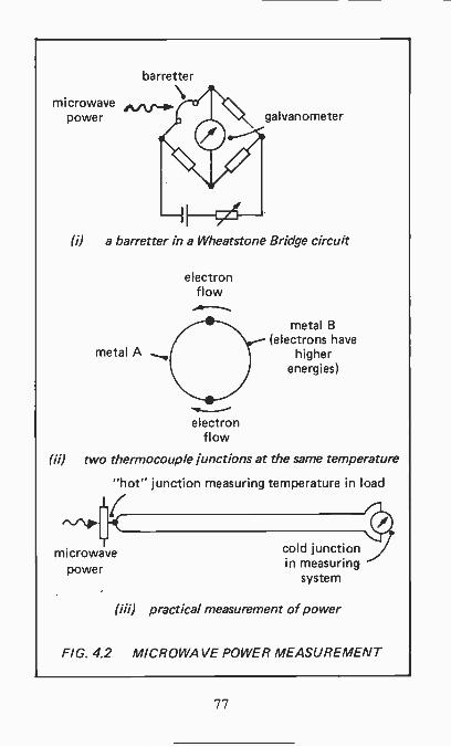
microwavepower galvanometer

(i) a barretter in a Wheatstone Bridge circuit

metal A

electronflow

electronflow

metal B(electrons have

higherenergies)

(ii) two thermocouple junctions at the same temperature

"hot" junction measuring temperature in load

.1(

T41(

microwavepower

cold junctionin measuring

system

(iii) practical measurement of power

FIG. 4.2 MICROWAVE POWER MEASUREMENT

77

00

(i)at

tenu

atio

n m

easu

rem

ent

0

netw

ork

unde

rm

icro

wav

ete

stge

nera

tor

e.g.

kly

stro

nm

odul

ator

lkH

z sq

uare

-wav

eos

cilla

tor

One

twor

kun

der

test

0

a/

mat

ched

mea

sure

men

tlo

ad-4

--w

ithou

tne

twor

k

load as

abov

e

dete

ctor

I.f.

atte

nuat

or

netw

ork

inse

rted

I.f. a

mpl

ifier au

dio

met

er

(ii)

esse

ntia

l fea

ture

s of

a m

easu

ring

syst

em

FIG

. 4.3

MIC

RO

WA

VE

AT

TE

NU

AT

ION

ME

AS

UR

EM

EN

T

"hot" junction senses the temperature of a load in whichthe microwave power is dissipated [see (iii) of the figure] .The "cold" junction temperature must of course be keptconstant. The heating takes time to settle down, hencethermocouple microwave power meters have slow responsetimes, e.g. from a few tenths of a second up to several seconds.However, they have good sensitivity.

4.3 AttenuationIn general attenuation is the reduction in magnitude of signalpower as it travels over a transmission path. It is solely due tothe resistance present and can be expressed as the ratiobetween the output power of a network and that at the input.Measurement of the attenuation of a network is usuallyaccomplished by measuring the power (P1) from a signalsource then measuring a second time (P2) with the networkinserted as shown in Figure 4.3(i). The signal source and itsload are matched. The network attenuation is then calculatedfrom 10 log (Pi /P2) decibels.

The bare bones of a practical system are shown in (ii) ofthe figure. This uses the above substitution method but forconvenience of measurement first modulates the microwavesignal by, for example, a 1 kHz square wave, thereafter theequipment works at this lower frequency. The signal beingused to determine the network attenuation is therefore a seriesof bursts of microwave power at the test frequency occurring1000 times a second and it will be seen that with a detector ofthe barretter type, the measurement at the end of the chaincan be at an audio frequency.

This is a circuit in all simplicity, a complete system provid-ing high accuracy also involves isolators, tuners and standing -wave indicators with a microwave frequency measurementsystem also built in.

79

Chapter 5

THE MAGIC OF MICROWAVES -COMMUNICATION SYSTEMS

Communication they tell us is the science and practice oftransmitting information, all very straightforward when we aretogether, but when apart, especially a long way, then weexpect telephone calls to be cheap and plentiful, televisionlikewise and we even need to learn of the problems of theworld "live by satellite". Microwaves play an important partin all of this. But how do we get from A to B by microwavewhen A and B are a long way apart? Certainly not by wave -guide as a glance at Figure 2.5 will show, cost and complexityare too great. Circular waveguides may have been used forlong distance telephony not so long ago, but these are noweclipsed by the optical fibre. Coaxial cables are less costlybut as Section 2.2 shows they give up at frequencies aboveabout 3 GHz.

There is only one transmission medium left and fortunatelyit is the least expensive of all - the space around us. Hencemost microwave communication is by radio. However,although true space does not attenuate a radio wave, theearth's atmosphere and the earth itself do, so we find that howa microwave travels depends greatly on these two factors andaccording to the wave frequency.

5.1 PropagationRadio transmission of microwaves is accomplished basically intwo different ways. We can see this for ourselves from thetelevision antennas, those for UHF stations (Fig.1.2) point toa local television transmitter, the others for SHF transmissionspoint up into the sky to a far distant satellite. To appreciatethe difference we might usefully start at the lower frequenciesand work upwards.

5.1.1 The Ground WaveThe energy radiated by most broadcast radio transmitters (thisdoes not include satellites) consists mainly of a ground wave

81

which travels over the earth's surface and a sky wave whichtravels via the atmosphere. The earth is an electrical conduc-tor and as the ground wave moves over it, charges are inducedin the ground and these charges travel with the wave. Amoving charge is an electrical current, hence power is dissi-pated and this power can only come from the wave whichtherefore is attenuated. How far away from the transmittera useful radio signal can be picked up depends mainly on thetransmitting antenna power output, its directional propertiesand in a rather complicated way on the frequency, the higherthis is, the greater the rate of attenuation of the wave.

Above about 1 - 2 MHz the ground wave is attenuated sorapidly that it is of little use except over short distances. Thisis why at the lower microwave frequencies (say UHF) tele-vision distributed by ground wave has a small service area andmany transmitting stations are required to cover even a smallcountry (e.g. over 600 for the UK). There are, of course,many other services which employ short distance ground wavecommunication, especially mobile ones. So we might con-clude (with tongue in cheek) that the UHF band (300 MHz -3 GHz; Sect.1.5) is usable for ground wave propagation butbecause of ground losses, the SHF band (3 - 30 GHz) is not.

5.1.2 The Sky WaveBelow the microwave range, say up to about 70 MHz, radiocommunication is possible by using a wave projected upwardsby the transmitting antenna into the ionosphere and reflectedback to earth. In this way the wave effectively skips over theground instead of travelling in contact with it. The ionospherewhich is a layer of ionized atmosphere some 50 to a few thou-sand kilometres high causes refraction of electromagneticwaves and effectively bends them back to earth. The effectvaries with wave frequency and many other factors. It doesnot really concern microwaves for their frequencies aresufficiently high that the waves pass straight through theionosphere with little refraction, this is just one of the reasonswhy satellite transmission is in the SHF range (see also Sect.5.3.2).

There is also tropospheric propagation (up to 10 km high)and this does extend into the microwave band, up to some

82

30 GHz. It is such a volatile transmission path however thatit is not a serious contender for normal microwave communi-cation systems.

5.2 Point -to -Point Microwave CommunicationWhat is generally referred to as a telephone network carriesmuch more than ordinary telephone conversations, the net-work also conveys telegraph, computer, facsimile and otherdigital data, radio and television baseband signals (basebandrefers to the range of frequencies initially generated, e.g. theoutput of a microphone or television camera). It is theavowed intention of the information technology people thatthese auxiliary services will increase abundantly so perhapsthe overall title "telephone network" is not so appropriatenowadays. However, to replace it is not easy. The termpoint-to-point encompasses all the services mentioned, so itis used for the title of this section. This is not to say thatother systems such as radar and electronic warfare do nothave their point-to-point features but for convenience weagree that here the term refers to whatever happens on atelephone network.

Point-to-point microwave transmission is seen in many largecities in the shape of a very tall tower fitted with microwaveantennas. Such for example is the Telecom Tower in London,this houses the microwave transmitters with waveguide feedsto the antennas which are on the outside, each pointing to itspartner antenna up or down country. As with light, nothingmust block the beam, so the tower is of sufficient height toclear all buildings and other obstacles. The maximumdistance tolerable between a microwave transmitter and itsreceiver is limited by the curvature of the earth as illustratedin Figure 5.1(i) and there is a further limitation caused bymist and rain. At microwave frequencies the wavelength maybe of the same order as the diameter of droplets, hence thereis some absorption and scattering so allowance must be madefor the worst atmospheric conditions. Although point-to-point microwave systems have carried telephony and tele-vision channels successfully for many years, high maintenancecosts of the antennas and the advent of better technology

83

00

Nar

ease

rved

stra

ight

-line

radi

o be

amB

A c

an c

omm

unic

ate

with

B b

ut n

ot w

ith C

beca

use

the

eart

h ge

ts in

the

way

(i)

surf

ace

ofth

e ea

rth

dist

ance

lim

itatio

n du

e to

cur

vatu

re o

f ear

th's

sur

face

mic

row

ave

links

(ii)

mic

row

ave

path

s in

tele

visi

on b

y sa

telli

te

FIG

. 5.1

CO

MM

UN

ICA

TIO

N B

Y M

ICR

OW

AV

E

broa

dcas

tsa

telli

te

(e.g. optical fibre transmission) are likely to lead to theirreplacement as time progresses.

Satellite transmission follows the general principles outlinedabove. Figure 5.100 shows the basic system. It is trulypoint-to-point on the way up but for television a slightlydivergent beam is used when the satellite transmits the signalback to earth in order to cover a certain area, e.g. a smallcountry. There is nothing in pure space to attenuate the wave,but there is some loss through the earth's atmosphere.

5.2.1 Assembling the PackageIf calling whatever is to be transmitted by microwaves apackage, be it analogue or digital and for telephony, television,data, etc., then for transmission over a microwave link it isperhaps obvious that the package can occupy a wide frequencyband, even up to some 100 MHz. A band like this can trans-port over 20,000 telephone conversations at the same time!A single telephone channel needs no more than 4 kHz band-width and a colour television signal some 6-7 MHz (band-width is considered in Appendix 3) so it is obvious that manycircuits can be assembled together to form a single package fortransmission over a microwave link. This might operate forexample through two pairs of dish antennas on the groundas in Figure 2.7(i) or over a satellite link as in Figure 5.1(ii)in which case the down link is also point-to-point.

We touched on the principle of "mixing" two frequenciesto provide a third, their sum or difference in Section 3.5. Onthis technique is based the method of assembling individualchannels to form a complete package to be carried on a micro-wave link. How single telephone channels find their way intoa microwave package is explained in essence below. A 4 kHzspeech channel mixed with a 104 kHz oscillation will produceamongst others a range of frequencies running from 100 to104 kHz. A similar speech channel mixed with 108 kHzresults in a band 104 to 108 kHz. These two higher frequencychannels can be combined and provided that there is no non -linearity, they will not intrude one upon the other just asbroadcast radio transmissions do not normally interfere. Agroup of 12 speech channels raised to a band 60 - 108 kHzmay further be frequency converted with other groups to

85

higher frequencies still and so on until a package of therequired size is formed. The system is known as frequencydivision multiplex.

Digital signals from computers, facsimile machines or fromspeech which has been converted into digital form are treateddifferently. Then time division multiplex is used in whicheach channel is allocated a different time interval for its trans-mission. All channels are examined in rotation and at eachinstant of time the signal from only one channel is transmitted.

Summing up, a package may contain a mixture of analogueand digital signals, each occupying its own individual fre-quency band of the width required. The whole package canthen be carried by a microwave radio signal.

5.2.2 Modulating a Microwave CarrierCommunication by radio invariably embraces modulation (seealso Appendix 3) which is the way we impress informationonto a carrier wave. Here the carrier wave is usually a sinewave at microwave frequency whereas the modulating wave isat a considerably lower frequency and may be extremelycomplex, consisting of speech, pulse, television waveforms or amixture of all.

Of the several different ways of impressing a signal onto acarrier wave, frequency modulation (f.m.) is almost invariablyused for microwave systems. It has several advantages over itsforerunner, amplitude modulation (a.m.) especially in that itis less affected by radio path noise. However, for the sameinput signal a wider carrier bandwidth is required. Happilysufficient bandwidth for large multiplex systems is availablein the microwave range.

With frequency modulation the carrier wave (in this casethe microwave) is of constant amplitude and its frequency isvaried about the mean value in accordance with the amplitudeof the modulating wave while the rate of variation is at thefrequency of the modulating wave itself. Of the many typesof modulator in use, the simplest to understand is that of anoscillator circuit tuned by an inductance -capacitance (LC)network with the frequency variation arising from changes inthe tuned circuit capacitance. Such capacitance variationsmay be developed by the connection of a varactor (variable

86

-I input,modulatinc

voltage

output

frequencydetermining

network(tuned circuit)

varactor

(i) a Hartley oscillator with added varactor

inputmodulating

voltage

output

(ii) voltage control of a multivibrator

FIG. 5.2 FREQUENCY MODULATORS FORMICROWAVES

87

capacitance diode) in parallel with the tuned circuit as shownfor a Hartley oscillator in Figure 5.2(i). The modulatingvoltage is applied to the varactor, hence the net tuned circuitcapacitance and therefore the oscillator frequency vary insympathy.

Slightly more complicated is the multivibrator circuitshown in outline in (ii) of the figure. The levels at which thetransistors switch are controlled by the input modulatingvoltage, hence the output frequency changes accordingly. Thecircuit may not be designed at microwave frequency but at alower one, stepped up as required by a frequency multiplier.When integrated circuits are involved, an operational amplifiermay be used to replace the multivibrator.

5.2.3 TransmissionThe modulated carrier, raised suitably in level by a poweramplifier is fed via a waveguide to a parabolic antenna forlaunching into the atmosphere. Over a ground link there isthe restriction on path length as illustrated by Figure 5.1(i)and also as mentioned in Section 5.2 there is a signal losscaused by mist and rain. Generally, therefore, "one hop"path lengths do not exceed about 60 km. For systemlengths greater than this (and many are), repeater stationsare used, usually evident as a tall mast with receiving dishes onone side and transmitting dishes opposite. These receive theweak modulated microwave signal, amplify it and then by useof a mixer (Sect.3.5), change the carrier frequency to oneslightly different from the received one. The new carrier isamplified and then transmitted onwards. Typically a 4 GHzincoming signal may be re -transmitted on 4.2 GHz. Thechange in frequency is required because some of the high-leveloutput signal may find its way back to mix with the low-levelinput signal. If both are at the same frequency, instability islikely to occur. The change in frequency greatly reduces therisk of instability. There may be many repeater stations enroute and at each successive one the frequency shift is reversed.

When the microwave signal finally arrives at its destinationit is collected over the area of a parabolic receiving dish andreflected into a waveguide. Filtering and mixing produce anintermediate frequency (say, 70 MHz) for further amplification

88

and limiting. Limiting cuts off all wave excursions above apredetermined level so that variations in amplitude are mostlyremoved, hence reducing noise. This can be done with fre-quency modulation systems because the amplitude of thesignal carries no information. The signal is then demodulatedso that the original band of modulating frequencies is regained.With a frequency modulated wave a frequency discriminator isrequired. A circuit commonly used firstly expresses thefrequency deviation of the frequency modulated signal as aphase -shift, then as an amplitude variation, i.e. the circuitoperates as an f.m. to a.m. converter. A conventional a.m.detector then produces an output at the modulation frequency(see also Sect.3.4.1). After amplification the demodulationproduct (which is a copy of the original package) is divideddown by the use of band-pass filters into its componentcircuits for transmission to the various destinations.

This is for one direction only, e.g. A to B. Many circuitssuch as those carrying television baseband data are trans-mitted in one direction only, others, for example, speechcircuits are two-way, hence a return circuit (B to A) is alsorequired. With such a system as described above, B to A isidentical with A to B and usually exists side -by -side with it.Thus the last repeater station in the A to B direction is alsothe first in the B to A direction.

5.2.4 Mobile CommunicationsWith point-to-point communication, when one station is

mobile a whole host of additional problems arises. No longeris the stability of a pair of wires (or channel in a fibre -opticsystem) from the telephone exchange to the user's telephoneavailable but instead a radio path. The radio signal has toenter buildings, go up and down hills, fmd its way throughstreets, avoid trees and generally cope with the fact that thereceiving antenna is low down, could be anywhere in the areaand even on the move on a vehicle. Given all this and everyone of these conditions has to be met, are microwaves of anyuse and if so, what range is suitable? We can make somerough estimates.

89

5.2.4.1 Frequency ConsiderationsA frequency modulation system is preferred and this in factrequires a greater bandwidth per channel compared with anamplitude modulation system, something approaching 30 kHzis needed, i.e. the channels need to be spaced at least 30 kHzapart (Appendix 3). Each radio channel must be duplex sothat conversation in both directions at the same time ispossible. Needing perhaps over 600 duplex channels on asystem so that most users can be accommodated when they allcall or are called together leads to a frequency bandwidthrequirement of, say, 40 MHz. The indications are that onlymicrowaves can provide bandwidths of this order, especially ifseveral radio carriers are needed to cover a large area.

Returning now to basic theory, it can be shown that whentransmitter and receiver antennas are dipoles, the powerdelivered to the receiver varies inversely as f2 where f is thefrequency, for example if f rises from 100 MHz to 1 GHz thereceived power is reduced by 20 dB (more on decibels inAppendix 1). However, it can also be shown that antenna gainvaries directly as f 2, hence these two frequency conditionstend to balance out. From this it appears that the highermicrowave frequencies with their abundance of bandwidthcan be employed - but there are overriding factors, twowhich perhaps place the greatest limitations are:

(i) buildings and trees - the signal has to find its way insidea building. Experimental work on the attenuationsuffered by an electromagnetic wave when passingthrough a brick wall shows that it may be a few decibelsat frequencies at low megahertz but can be as much as40 dB at 3 GHz, clearly at this latter frequency gettingthrough a wall is difficult, at even higher frequenciesalmost impossible. We have more evidence of this in thefact that at the higher still frequencies of light it is mani-festly impossible. Tree losses also increase with fre-quency and above 1 GHz dense trees are a majorobstruction to a wave.rainfall - we can guess from the effects of rainfall onlight that microwaves, although of somewhat lowerfrequencies will also be affected. It has been estimated

90

that in heavy rain an attenuation of 0.01 dB/km at 2GHz rises to around 10 dB/km at 20 GHz. Even moder-ate rainfall attenuates a 20 GHz wave at a rate of 3dB/km.

Putting (i) and (ii) together indicates that the higher micro-wave frequencies are unsuitable for mobile communications, acompromise between the conflicting requirements appears tolimit the use of the microwave spectrum to the UHF band, i.e.to frequencies below about 3 GHz.

5.2.4.2 The Cellular SystemWe have seen from Section 5.1.1 that microwaves at the lowergigahertz frequencies are capable of serving no more than arelatively small area unless very high transmitter powers areused. In open areas things are not so bad but in heavily built-up urban areas the received signal can be as much as 60 dBlower. Accordingly the cellular system has been developedwith considerable success, but it must be admitted that thisdepends heavily on microprocessors and large-scale integration,in fact until these came along the service could never have gotoff the ground. An idea of the method can be gained fromFigure 5.3. The service area is divided up into a number ofcells (hence the description of the system), cells of the samenumber all working on the same group of microwave fre-quencies. The drawing shows the cells to be of similar areabut of course in practice they may differ widely in size. Thenumber of different cells is shown as 7 but the actual numberemployed depends on the type of area to be served. Theconnections are shown between non -mobile and mobilesubscribers, this of course does not rule out connectionsbetween two mobile subscribers. It must be emphasized thatthis is the basic idea only, many variants exist and manymore will be developed.

Each cell contains fixed transmitting and receivingantennas, the transmitter radiating sufficient power (severalwatts) for the complete single cell and supplying all cells ofthe same number as shown. Interference between cells work-ing at the same frequency is minimized because of the rapidattenuation of the wave with distance. Throughout each cell a

91

to remainingcells numbered

61I

voice andcontrol

channels

to allcells

numbered

1 2 3 4 5

I I I I I

I I II i

7

mobile telephoneswitchinc centre

Avoice

0 circuitsIf

main telephonesystem

switching centre

5

st2

6

area ofland

selectedas one

cell

servicearea

non-mobilesubscribers

I microwavedirectional

antenna

FIG. 5.3 TYPICAL CELLULAR SYSTEM LAYOUT

92

satisfactory service should be available. However, when avehicle moves across the boundary from one cell to an adjoin-ing one its own transmitter and receiver are automaticallyrealigned to the frequencies of the new cell. This of courseis no mean feat. Firstly the controlling computer must knowthe location of each mobile telephone. It is the signal-to-noiseratio (Appendix 2) on the radio path which is the main deter-minant of the intelligibility of the signal it carries, this musttherefore also be checked, with the system able to switch themobile receiver frequency to the new one as quickly aspossible, say within less than 40 ms. All this requires a separ-ate data link with the mobile system, the same link is alsoused for setting up and terminating calls.

5.2.4.3 Reducing Signal FluctuationsIf we consider a vehicle moving along a street dominated bybuildings, it is clear that a microwave signal being received ortransmitted will suffer uncommonly large amplitude vari-ations including short -duration fades. Signal variations ofgreater than 20 dB may be expected. Fortunately the major-

to almost a complete loss of signal are of veryshort duration, the actual duration decreasing with the speedof the vehicle for example, fades of 10 - 20 ms at 4 mphfalling to only a few milliseconds at 20 mph. Even thoughthese times seem short, overall such variations must result inan unsatisfactory signal-to-noise ratio, hence without correc-tion the degradation in voice transmission could be serious,for data transmission, disastrous.

A considerable improvement is obtained by using adiversity system. This employs two or more cell antennas forboth transmit and receive with directional characteristics asrequired. It is possible then for the receiving equipment ineither direction to switch to the antenna providing the highestsignal-to-noise ratio or alternatively the outputs of theantennas can be combined on the assumption that, eventhough spaced only a wavelength or more apart, they areunlikely to experience signal fades at the same instant.

Voice processing might also be employed. Telephonemicrophones vary in their sensitivities, talkers vary far morein their voice levels and how far away from the mouth the

93

handset is held. The system therefore has to accept lowelectrical speech levels from weak voices at large speakingdistances to high levels from loud voices close to the micro-phone - this could easily be a range of up to 60 decibels.Such a range would create difficulties in the modulation ofthe frequency modulation carriers, low voice signals resultingin a reduction in channel clarity, high ones experiencingclipping.

Much can be done to improve the signal-to-noise ratio andhence ensure good overall transmission quality, especially by:

(i) pre -emphasis and de -emphasis - by this method the highvoice frequencies are raised in level before modulation inthe transmitter (pre -emphasis), then reduced in thereceiver by the same amount (de -emphasis) so that over-all a flat response is obtained. By increasing the higherfrequencies during pre -emphasis the signal-to-noise ratioover the channel is improved and this is maintainedduring de -emphasis because the reduction in noise is thesame as that of the signal.

(ii) companding - is another system for improvement of thesignal-to-noise ratio over a channel. The voice frequen-cies generated by a talker firstly meet a volume compres-sor which provides more gain for low amplitude signalsthan for high amplitude ones. Low-level signals aretherefore less affected by noise on the channel becauseof their increased amplitudes. At the receiving end avolume expander restores the voice signal to its originalrange of amplitudes.

Both (i) and (u) may be used together with the result thatmuch of the variability of the microwave link is ironed outand users experience satisfactory transmission quality. Thesefew notes which are mainly restricted to how it is possible totalk over a mobile system are only sufficient to give us aninkling of the complexities involved. The control system alsois indeed a frightening collection of integrated circuits for itmust at least (i) know where every vehicle is, (ii) determinewhether it is available to receive a call, (ii) transmit that call,(iv) respond to a mobile originated call, (v) switch to a differ-ent transmitter when a vehicle moves across a cell boundary,

94

(vi) handle the transfer of calls to and from the main telephonesystem.

5.3 Broadcast CommunicationBroadcast as opposed to point-to-point simply implies a widedissemination of information. As far as microwaves are con-cerned television reigns supreme in the broadcast field. Herewe consider only the two types of television broadcast systemsgenerally entitled "terrestrial" (the wave travels over theground) and "satellite" (the wave travels down from a high-flying satellite).

5.3.1 Television (Terrestrial)Section 5.1.1 shows how a ground wave is attenuated andsuggests that at frequencies higher than UHF the ground wavehas little to offer. Accordingly some terrestrial television isbroadcast in the VHF band (30 - 300 MHz) but most is at ahigher frequency at the lower end of the UHF band (300 MHz- 3 GHz). However, there is some help from experimentalwork which has shown that wave energy lost to the grounddecreases with height above the ground to the extent that atheights of several wavelengths the wave suffers very little. Infact the strength of the ground wave transmitted from a half -wavelength dipole varies directly with ht x h, where ht is theheight of the transmitting antenna and h, that of the receivingantenna. Thus some improvement in the received signal isobtained from siting television antennas high on roofs. Neverthe-less because of other obstacles such as hills and buildings andthe fact that as frequency rises smaller objects such as treesand leaves create absorptions, we can sum up with the conclu-sion that in terms of the microwave range terrestrial televisionis limited to the lower end [see Fig.1.2(ii)] .

At the transmitter the power amplifier is most likely to be aklystron (Sect.3.2.1) with its output fed to the antenna by awaveguide (Sect.2.3). The main type of antenna used forreceiving is well known and easily recognized as a Yagi (Sect.2.4.1) with a coaxial lead to the television receiver. Indoor orset -top receiving antennas may also be used in strong signalareas.

95

5.3.2 Television (Satellite)Without microwaves there would be no satellite television atall so perhaps our first consideration should be the fact thatmicrowaves can reach up to satellites whereas waves of lowerfrequency cannot. This involves looking a little more closelyinto the effect the ionosphere has on waves of different fre-quencies. The ionosphere (first mentioned in Sect.5.1.2) arisesfrom the ionizing influences of solar radiation. This acts onparticles in the atmosphere and supplies energy to electronsenabling them to escape from their parent atoms which arethen left positively charged and known as positive ions. Afree electron may subsequently combine with a neutral atomor molecule to form a negative ion. The concentration of ionsin the ionosphere is extremely variable, changing with dayand night, season, height and sun -spot activity. Satellite tele-vision is in the SHF band (3 - 30 GHz) and what is so helpfulabout the ionosphere is that it does not refract these fre-quencies and return them to earth as it does certain lowerfrequencies.

Surely none of us has escaped the standard school physicsexperiment of dipping a stick into water and finding that itappears bent. This is because the velocity of a wave in thedenser of the two media (air and water) is lower and it iseasily shown that this results in the wave being deflected or,as we say, refracted. We assess this by the refractive index(.4) which is simply the ratio of the wave velocities in thetwo adjacent media. When p. = 1 there is nb refraction.

Ionization changes within the ionosphere can be consider-ed as adjacent media of different densities, hence as a waveprogresses through the ionosphere it can experience continualrefraction and under certain circumstances be deflected backto earth. This is the opposite of what is required for satellitetransmission for it is essential that the wave gets through tothe space beyond where there is nothing to interfere with itsprogress no matter how long the journey. The mathematicalformula which sorts this out is more than a little complex butby making several assumptions (e.g. that there is no magneticfield present and there are no particle collisions) it is possibleto indicate what happens as frequency rises. Clearly µ mustbe as near to 1 as possible for the waves to go straight through:

96

Refractive Index, µ = N/1 - (cNniax/f 2)

where f is the frequency under consideration and Nmax isthe maximum electron density. Clearly from this, as fincreases, 12 approaches unity and any refraction of the waveis reduced. Of course there are so many variables around(especially Nm) that the formula can only be taken as aguide yet it is sufficient to indicate how microwaves are usablefor satellite television whereas lower frequencies are not.Generally in Europe the frequencies employed are around12 GHz.

To see how microwaves function in satellite television letus follow them on their journey from camera to television set.The baseband frequencies from the camera and microphoneoccupy a bandwidth from 0 to 6 - 8 MHz. This band fre-quency modulates the microwave carrier (say around 12 GHz)resulting in a microwave signal of up to some 27 MHz band-width centred on the carrier frequency. The increase in band-width follows from the need to accommodate sufficient of theharmonics produced in the modulation process. After modestpower amplification (a few kilowatts) by a klystron or travel-ling wave tube, the signal is conducted by waveguide to thetransmitting antenna. The antenna will be basically of para-bolic shape [Fig.2.7(ii)] aimed at the satellite. On its journeythrough the earth's atmosphere the microwave signal sufferssome absorption, refraction and scattering but the transmitterpower is such that a signal of ample strength arrives up there.

Most satellites are in geostationary orbits (stationary withrespect to earth), positioned at nearly 36,000 km verticallyabove the equator and travelling at just over 11,0001cm/hour.At this height and speed the satellite completes one orbit inexactly the same time as the earth rotates once, hence to anobserver on earth the satellite appears to be stationary. Thesignal is received on a parabolic dish, amplified and frequencychanged so that up and down microwave frequencies differslightly to avoid instability. The signal is then power ampli-fied by a travelling wave tube and fed to the transmittingantenna by waveguide. This antenna is usually a single para-bolic or several working together, but for certain purposes ahorn antenna may be used, a type which can be likened to a

97

waveguide opened up into a horn shape, it of course does nothave the same high directivity of the parabolic.

Satellites are powered by the sun so the transmitter outputpower is limited, generally to no more than 200 watts. Thewave polarization will be vertical, horizontal or circular (Sect.1.4). On the journey down to earth there may be diffusionand absorption by rain, mist and clouds in the lower layers ofthe atmosphere which could account for a loss of severaldecibels. The strength of the signal picked up by a groundantenna (usually parabolic) varies with its size and dishes offrom some 30 cm up to 1.6 m are common, the larger sizesbeing required for reception from more distant or less power-ful satellites. Microwave signals received by the dish aredirected into a feed horn coupled to a low noise blockconverter (LNB). This device is a microwave frequencychanger which accepts the incoming band (or block) of signalsand changes them to a similar band but centralized on a lowerfrequency so that coaxial cable can be employed between theantenna and the satellite receiver instead of a waveguide (thecost of such an ungainly contraption would be prohibitive).The feed horn and LNB must be adjusted to match theincoming wave polarization and the output is likely to bebetween 1 and 2 GHz, which is still in the microwave range.However, a second frequency changing stage in the satellitereceiver results in a carrier of, say, 70 MHz, so at this pointthe microwave story ends. The 70 MHz signal is demodulatedto regain the baseband frequencies which then control thetelevision receiver.

98

Chapter 6

THE MAGIC OF MICROWAVES - RADAR

We might consider radar (an acronym from RAdio DetectionAnd Ranging) to have first seen the light of day in February1935 when Sir Robert Watson -Watt produced a notablememorandum entitled "Detection and Location of Aircraftby Radio Methods". The basic principle on which this wasfounded is the same today, that is if an aircraft or otherobject is irradiated with electromagnetic energy, a smallamount is re -radiated and can be detected. Furthermore, ifthe energy were to be transmitted in short high -power pulsesthen by measuring the time elapsing between transmittingthe outgoing pulse and receiving the reflected one, thedistance away of the reflecting object could be calculated.Very many refinements have been added to this basic idea asthe years have passed, perhaps the most fundamental onebeing the use of highly directional antennas so that not onlycan the distance away of the object be measured but also itsbearing.

Although the earliest experiments were conducted at about12 MHz, microwave technology has taken over since its veryshort wavelengths allow the use of small antennas and reflec-tions are more sharply defined. It is also found that signalsmay be returned from other than metal objects. Generallyradars operate at frequencies from 600 MHz to 40 GHz (50cm to 7.5 mm).

6.1 Reflection of Radio WavesSection 2.1.2 considers the reflection of electromagneticwaves, albeit in a much simplified fashion. We normally thinkof transmission lines as lengths of metallic conductors alongwhich a wave progresses. Now we must expand our thinkingto consider the atmosphere also as a transmission line for it isin fact a medium through which an electromagnetic wave istransmitted. It has its own characteristic impedance (Z0) andother constants. For the more technically inclined the

99

characteristic impedance of free space is given by V(µ0/e0)where pto is the magnetic constant of free space (4ir x 10-7H/m) and eo is the electric constant (8.854 x 10-12 F/m).This gives the value of Zo as 376.7 ohms. The atmosphere hasits own characteristic impedances not greatly different fromthis but varying with its make-up.

When radio wave energy therefore meets a discontinuity inthe atmosphere (i.e. anything which has not the same charac-teristic impedance as the atmosphere), some energy is reflectedback along the transmission line, in other words it is returnedto the transmitter. The likelihood of any solid mass in theatmosphere having the same characteristic impedance as theatmosphere itself is practically zero, hence radar relies on theprinciple that an object will reflect some of the wave whichhits it.

6.2 The Radar Range EquationAlthough much of what is considered in this section may tosome be obvious, this interesting equation is developed toprovide useful reminders of the difficulties with which theradar designer has to grapple. That so much success has beenachieved is demonstrated by the fact that nowadays a missilecan use its radar to catch up with another one. The theory isat its best only a guide because so many of the factors affect-ing the distance over which a particular radar system canoperate are exceedingly variable. The concept of the isotropicantenna may seem to some a little strange so we take this firststep by step.

The isotrophic antenna is a purely theoretical idea develop-ed for assessing the usefulness of -practical antennas. Theisotropic is considered to be a point source radiating equallyin all directions, hence if, for example, a transmitting antennaradiates an electromagnetic wave power of Pt watts then atany distance R metres away this power can be considered asbeing spread over the surface of an imaginary sphere of radiusR. Hence the power flux density (p.f.d.) R metres away isPt/4rrR2 watts per square metre (W/m2) as developed inFigure 6.1. The gain of any practical transmitting antenna in agiven direction is then given (usually in decibels) by:

100

Power radiated =Pt watts

Area =1 squaremetre

Sphere of Area of surface =

Rrmetradius 4trR2 square metres

es

Isotropic Antenna(point source which

radiates equallyin all

directions)

Power over 1 square metre =

Pt4TrR2

i.e. power flux density at surface ofsphere

pfd - watts per square metre (W/m2)47TR2

FIG. 6.1 RADIATION FROM AN ISOTROPIC ANTENNA

Gt =power radiated by the antenna

power radiated by an isotropic antenna suppliedwith the same transmitting power

Equally the gain of a receiving antenna, Gr, is measured as:

Gr =signal power delivered by the antenna

signal power delivered by an isotropic antennafor the same transmitted power

Consider a target at a range R in free space. As shownabove the p.f.d. at R will be

Pt

4irR2

101

for an isotropic antenna but

Pt Gt

47rR2

for a practical antenna of gain Gt.Now suppose that the target intercepts this power over an

effective area of a square metres and re -radiates it back overthe same distance R to the receiving antenna:

PiGttotal power re -radiated (reflected) = x a .

477R 2

The p.f.d. at the receiving antenna is derived by assuming thatthe target is now a transmitter, hence:

PtGtap.f.d. at receiving antenna = W/m2(47rR 2 )2

Suppose that the effective area of the receiving antenna isA, and that its gain relative to the isotropic is Gr, then:

signal power output, Pt of receiving antenna

PtGta

(4nR 2 )2x Ar watts .

Ar is related to the gain by the basic antenna formula:

Ar47r

PtGtaGrX2i.e. Pr = x watts

(47r/2 2 )2 47r

GrX2

and if, as is most likely to be the case, the same antenna is

102

used for both transmission and reception, Gt = Gr (= G),hence:

Pr -(47)a R4

ptG2ax2watts .

There will be a minimum value for Pr for the receivingsignal to be usable, say, .(min), hence by rearranging:

PtG2aX2R=

(4703 Pr(min)

Note the variables:

1/4

metres.

(i) the formula assumes free space, atmospheric path loss isnot included;

(ii) Pronin) is controlled by system noise which is notoriousfor its variability;

(iii) a is perhaps the most variable quantity of all as wemight expect. For a large jet aircraft head on a mightbe around 10 but side on as much as 100 times greater.Small aircraft show an even greater variation.

Many other variables are also present so we must concludethat accurate calculation from this simple formula is notpossible, but it is useful as a guide. Nevertheless two impor-tant features the formula does bring to notice are that:

(i) R varies as the fourth power of the transmitter, hencelarge increases in Pt are required to increase R evenmoderately, e.g. doubling Pt increases R by less than20%.

(ii) Technically R increases as the square root of the wave-length. It would appear therefore that the range isincreased by lowering the frequency, perhaps belowmicrowave. However, changes in A have a considerableeffect on the size and design of the antenna so a com-promise has to be adopted.

103

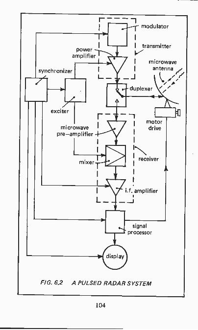
poweramplifier

synchronizer

exciter

microwavepre-amplifier

L

mcdulator

I transmitter

microwaveantenna

-J /r/\.-duplexer

r- -motordrive

receiver

i.f.amplifier

mixer

signalprocessor

FIG. 6.2 A PULSED RADAR SYSTEM

104

6.3 Elements of a Radar SystemRadar might be defined in a few words as a system for ascer-taining simply the presence or more likely the direction andrange of objects such as aircraft, ships and buildings. A

typical basic pulsed radar system capable of satisfying theserequirements is illustrated in Figure 6.2. Many moderntechniques such as are used in navigation, weather prediction,astronomy, early warning air and sea surveillance and evenmissile destruction may all be highly sophisticated systems yetthey are merely extensions based on this moderately simplearrangement. Needless to say, computer technology aboundsin plenty. The system shown in the figure is, of course,static, when it is built into a moving object such as an aircraftor a missile then things really do get complicated.

It all starts with the synchronizer, the function of which isto control the timing of the whole system. To sand out aradar pulse the synchronizer causes the transmitter modulatorto send out a high voltage pulse to the power amplifier whichmay be a klystron (Sect.3.2.1) or for the higher powers, amagnetron (Sect.3.3.1) or sometimes a travelling -wave tube(Sect.3.2.2). At the same time the synchronizer triggers theexciter into applying a microwave drive signal to the poweramplifier, the net result being a high power microwave pulsefed from the power amplifier to the duplexer via a waveguide.

The duplexer is basically a send/receive switch, essentialwhen a single antenna is employed for both transmission andreception. It also has the function of protecting the receiverfrom the high power of the transmitter. It must operatewithin the time between transmission of the outgoing pulseand reception of the echo. The one shown in Figure 6.2 isdepicted as a mechanical switch but it is obvious that theswitching speeds required are beyond the capabilities of amechanical device. Several different types of duplexer are inuse, a ferrite circulator as discussed in Section 2.5.2 is perhapsan obvious choice, such devices can handle the very hightransmitted power levels and provide some 20 - 30 dB attenu-ation between transmit and receive. A type also commonlyused is the gas -tube which is inserted within the waveguidesystem. On receiving the low powered signal passes throughthe tube unattenuated but the high power of the transmitter

105

causes the gas to ionize and its resultant low resistance short-circuits the r.f. energy and prevents it from affecting thereceiver. Two gas -tubes in a hybrid arrangement are requiredfor a complete balanced duplexer. More recently high powermicrowave diodes are coming into favour as replacements forgas -tubes. Via the duplexer therefore a single pulse of micro-wave energy is radiated. In the drawing the antenna is shownas being steered by a motor drive, equally a stationary antennamay be used with the beam steered electrically.

The reflected signal is received by the antenna, it is directedto the receiver via the duplexer. It is first amplified by a low -noise microwave preamplifier and then, using the superhetero-dyne principle converted to an intermediate frequency (Sect.3.5) for transmission to the signal processor. The localoscillation for the mixer is supplied at the correct time by theexciter. This is the ideal situation but usually many otherweak signals and noise (clutter) also arrive from the antenna sothe main purpose of the signal processor is to discriminateagainst the unwanted signals, obviously a complex computeroperation. The output is then fed to the display system, in itssimplest form a cathode-ray tube which gives a range -onlypresentation as sketched in Figure 6.3(i) but is more likelyto be of PPI (plan -position -indication) form indicating bothrange and bearing as shown in (ii), here the time base con-tinually rotates to correspond with the position of the antennaat any instant. Clearly the repetition frequency and length ofthe pulses must be such that the echo does not return afterthe following transmitter pulse for on a display as in Figure6.3(i) it might get lost in the transmitted pulse display or ifarriving later still may be mistaken for a short range echo ofthe second cycle.

6.4 Navigation and Electronic WarfareWe put these two sub -titles together because in general theyare both based on an extension of the radar principle so thatit applies to moving objects, i.e. either the observer or thetarget or both are in motion. Two examples only are: (i) thecontrol of aircraft from the ground; and (ii) one missile seek-ing out another. To do no more than examine the basic

106

signalstrength

transmittedpulse

(i) simple oscilloscopedisplay

270°

0°

90°

(ii) PPI display 180°

FIG. 6.3 RADAR DISPLAYS

107

principle is as far as we dare go, otherwise things become toocomplicated and lengthy. However, what follows should beenough for an appreciation of how the Doppler effect is usedwith microwave technology to measure speeds of distantobjects.

The Doppler effect is noticed as the apparent change inpitch of a sound wave from a moving body as it passes by(first considered by Christian Doppler, an Austrian physicist).The effect is not, however, limited to sound waves but occurssimilarly with electromagnetic waves including those of lightwhere slight changes in colour arise.

Consider the system in its simplest form as that of a radartransmitter of frequency ft radiating continuous waves (i.e.the pulse technique of Sect.6.3 is not used). The echo isdetected and mixed with a low-level sample of ft. It is perhapsobvious that if both the transmitting station and the target arestationary the echo will be at the same frequency as ft. How-ever, if one or both of these is moving the echo will have adifferent speed imposed upon it and there will be a differencein frequency between the transmitted and received signals (theDoppler shift). From the basic physics equation the radar onefollows:

Doppler shift, fd = ft+v)

1

(c - v)

where c is the speed of propagation of the transmitted wave(ft) and v is the radial velocity of the target. The formula canbe adjusted to account for movement of both transmitter andthe target.

Through a little juggling and approximation a very simpleformula arises:

2vfd ' -X

where X is the wavelength.Let us take for example an aircraft approaching a radar

station at a speed of 200 m/s (approximately 450 m.p.h.) andassume that in air c = 3 x 108 m/s. For a transmitted frequency

108

at 1 GHz, fd is calculated from both formulae to the nearestwhole number as 1333 Hz, so clearly the shdrtened foirilula Issufficient as a guide. Since in the practical case fd is easilymeasurable, v can simply be derived from (fdX)/2.

Many radar techniques are in use based on the general radarprinciples outlined in the preceding sections together with theDoppler shift technique so that radar technology has nowreached the point where practically any civil or militaryrequirement can be met.

109

Chapter 7

THE MAGIC OF MICROWAVES - HEATING

That microwaves are used for heating is known to all, especi-ally the cooks among us. In trying to understand theprocess, however, we ought first to understand somethingabout heat but when we do inevitably the term energy con-fronts us. Both terms abound in everyday conversation yetwe understand so little about what these two quantities reallyare. Certainly we have no real knowledge of what energy isand the dictionary gives little help for it explains energy awayas "the ability of matter or radiation to do work", i.e. interms of what it can do rather than what it is. Trying toexplain heat is also difficult for generally we find that heatis described as a form of energy.

Held in the hand a cricket or golf ball is no threat, but ifwe get in the way of one while it is in flight, it can do nastythings to us. What has changed? Nothing except that it hasbeen given a copious supply of Nature's mysterious quantity,the energy of motion - kinetic energy.

Atoms and molecules in all matter are continually in astate of vibration. They therefore possess kinetic energy. Ifheat is added the motion is increased so the kinetic energyincreases also. On the other hand if heat is removed themotion is reduced. Thus one way of describing heat is that inmatter it can be perceived as the kinetic energy of atomic andmolecular motion. Temperature is a measure of the average ofthis energy. Put simply, temperature does not measure theamount of heat in an object, it measures its hotness.

An electromagnetic wave has energy which can be trans-ferred to the vibrating particles in matter (atoms, electrons,molecules) through interaction with its electric and magneticfields. The energy is kinetic hence the vibrations increase andfrom our explanation above, heat is "generated". Infra -redradiation has long been used in this respect but now thenext -of -kin, the microwave does the job more efficiently.We examine the production of heat in a dielectric in moredetail in the following sections.

111

7.1 Charge DisplacementWe whose initiation included Ohm's Law and the subsequentformulae for power (E2 /R, I2R) may be excused for thinkingabout electrical heating in terms of a resistance wire glowinghot. But microwave heating has added another dimension, itactually heats a dielectric which from our knowledge ofcapacitors should never occur to any great extent. After all,the definition of a perfect dielectric is a material which acceptsno energy from an applied electric field and therefore it musthave infinite resistance and cannot heat up. Practical capacitordielectrics do have some charge carriers although in most cases,very few. An applied voltage therefore results in such a smallcurrent that electrical resistance heating is negligible.

Now we meet a different form of heating altogether, nolonger relying on the Ohm's Law type of free charge carriermovement but in fact operating on all the atoms or moleculesor both (for convenience let us call these particles) of thewhole material. Very briefly, when a suitable dielectric isplaced in an electrical field, charges within the particles aredisplaced and when the applied field is alternating the dis-placement follows the field polarity changes. To do thisenergy must be absorbed from the field and it is then dissi-pated as heat. When charges within a particle are displaced,the particle is said to be polarized. Different kinds of polariza-tion can arise but fortunately heat seems to be generatedwhatever happens. We look at the least complicated formonly, it will be sufficient to gain a good understanding ofmicrowave heating.

7.2 PolarizationWhen a dielectric is subjected to an electric field, the particles(atoms or molecules) become elongated in the direction of thefield, the electrons being pulled one way, the nuclei in theopposite direction as sketched in Figure 7.1(i). The chargeswithin each particle are now unbalanced to the extent that theends of it are oppositely charged - the particle is said to bepoled, it is called a dipole, the process being known aspolarization. Furthermore, each particle may be aligned in thedirection of the field, hence giving rise to a redistribution of

112

electron

\I I atom

nucleus

nucleus pulledthis way

electron orbitspulled

this way

4 -4 - ---/ \

- = - -+ atom -polarities

(i) creating an atomic dipole

strong electric fieldno electric field

(ii) dipoles responding to an applied electric field

FIG. 7.1 DIELECTRIC POLARIZATION

charge within the material as shown diagrammatically in (ii).Losses, appearing as heat occur in the dielectric because energyis absorbed from the electric field in aligning the particles. Ifthe electric field is reversed, the dipoles reform in the oppositedirection and if the field alternates at some high frequency,

113

the dipoles continually readjust, the energy dissipation result-ing in a continuous generation of heat - from within thematerial. The magnetic field of the electromagnetic wave hasan insignificant effect because there is nothing in mostdielectrics it can work on.

Even for this simplified explanation, the mathematics canget out of hand so we take the key dielectric heating equationonly. From this the important features can be seen:

power generated within a dielectric = 27rfE2c0watts per unit volume

where E is the voltage applied at a frequency f, co is theelectric constant (permittivity of free space) and 5 is theeffective loss factor. This latter term is not an easy one toget to grips with unless one has studied dielectrics in depth,it is technically the product of the power factor and therelative permittivity of a dielectric. For a given electric fieldthe heat generated is proportional to the power factor.However, its name gives us a clue for clearly the greater theoverall loss within a dielectric, the more the power which willbe absorbed from an electromagnetic wave. It is a summationof the various different losses and is both frequency andtemperature dependent.

7.3 Microwave Heating FrequenciesMost importantly the formula shows that the heating effect(power generated) varies with the frequency and with thesquare of the applied voltage. Considering now the practicalcondition, it is evident from the formula that too high avoltage is likely to lead to breakdown, better therefore to relyon a high value for f and this puts its value in the microwaveregion. Overall control is needed nationally since high powersat microwave frequencies are in danger of propagating electro-magnetic radiation which may interfere with television,medical or other scientific equipment. A list of microwaveheating frequencies has therefore been agreed.

It is clear from the formula that the product f x 5 is thefactor determining the wave voltage required for a given

114

degree of heating. As an example, most foods contain waterwhich it so happens has the highest value for 5 (about 16 at15°C at 3 GHz - for most dry materials 5 is less than 0.5),this most often leads to the choice of 2450 MHz (2.45 GHz)for domestic ovens, 896 MHz is also used although lessfrequently.

7.4 A Typical Microwave Heating SystemBecause most readers have experience of domestic microwavecookers it is propitious that this is the type we examine, safein the knowledge that basically industrial types are littledifferent. The microwave energy is radiated from an antennasystem into the free space within a closed cabinet whereuponit is absorbed by materials (dielectrics) having a high lossfactor, in the case of the domestic oven such a material ismainly the water contained within food. A typical domesticcooker closed cabinet might have the dimensions shown inFigure 7.2(i) with the general construction as sketched in(ii).

The closed cabinet is constructed of a conducting materialsuch as aluminium or stainless steel. These metals have almostzero loss factors so absorb no power, in fact practically all ofthe microwave reaching them is re -radiated. The cabinet maybe considered as a rectangular waveguide closed at both ends.Microwave energy fed in is continually reflected by the metalwalls in all directions and standing waves are set up with theirnodes and antinodes (Sect.2.1.2).

In the majority of microwave cookers the microwave poweris provided by a fan -cooled magnetron (Sect.3.3.1) and it isfed into the cavity via a short length of waveguide. The stand-ing wave patterns would normally cause uneven heating, thisis minimized by the mode stirring fan which consists of slowlyrotating blades which project the microwave energy in differ-ent directions to vary the field patterns. The item to beheated is placed on a motor -driven turntable, again to distri-bute the heat evenly. The door and its locks are so designedthat power is disconnected from the magnetron when the dooris opened. Door sealing is such that energy radiation into theopen air is prevented. The whole cooker may be rated at some

115

door

metalcabinet

typical cabinet dimensions

waveguide

-4-AzAP frommagnetron

mode (1:)stirrer

food orother

material

(ii) typical construction

turntable

FIG. 7.2 A MICROWAVE COOKER

1250 watts for an electromagnetic wave power of 650 watts.In industry the same principles may apply but the ovens are

naturally of larger dimensions, e.g. for defrosting food in bulk.

116

Tunnel ovens are employed in which the material moves alongthe tunnel on a conveyor belt (e.g. for curing rubber extru-sions, drying leather). Small but powerful ovens are used forheating resins and other chemicals.

7.5 Microwave DiathermyNever having considered ourselves to be dielectrics it maycome as a surprise to find that microwave diathermy (fromGreek, through heat) operates on the principles outlinedabove for microwave cookers. In this medical treatmentmicrowave energy is transmitted into the skin from a distanceof a few centimetres. The aim is to heat deeply placed muscle,not of course to cook it, hence precautions are built in sothat over -exposure to the microwaves is impossible. Bothpatient and physiotherapist wear wire -mesh goggles to excluderadiation from the eyes.

117

Appendix 1

DECIBELS

It may have had its origin in the era when scientists werebeginning to measure the intensity and other characteristicsof sound waves. It was then discovered that homo sapiensseemed to have logarithmic ears for the intensity of soundhad to be increased many times before it was considered tobe only twice as loud. A logarithmic system of measurementseemed to be the answer and it was soon found that usinglogarithmic units to express power, current or voltage ratioshas two distinct advantages: (i) large numbers are reduced andso become more manageable; and (ii) in a complex systemwith a large number of circuits, each contributing a gain orloss, calculation of the overall power, etc., ratio by multiplica-tion is unwieldy. By expressing each ratio in a logarithmicunit, addition takes the place of multiplication, a moremanageable process altogether. Hence the bel came on thescene (after Alexander Graham Bell, the Scottish -Americaninventor) which is simply the common logarithm (to the base10) of the power ratio. This gives rather low figures so anoffshoot soon appeared, the decibel (symbol dB) which isone -tenth of one bel. If the power, current or voltage inputto a circuit is given by P1, II or V1 respectively and thepower output by P2 12 or V2 then the attenuation (or gain):

P2 122 X Zn = 10 log -= 10 log = 20 log - dB

P1 /12 x Z 11

but note that Ii and 12 must be measured in the same termin-ating impedance, Z. Similarly:

V2n = 201og - dB

V1

and again the voltages must be measured in the sameimpedance. (Note however that we often deliberately go

119

astray when .quoting the voltage gain of an amplifier by usingthe above formula while ignoring differing input and outputamplifier impedances. No problem if we realize what we aredoing and tell others.)

If gains and attenuations are being considered together,then signs become necessary. If P2 is greater than P1, thereis amplification and n is positive, conversely if P1 is thegreater, there is a loss and n is negative. Suppose P1 = 1 mWand P2 = 0.5 mW, obviously there is a power loss so n shouldwork out to be negative:

attenuation in dB (n) = 10 log (P2/P1 ) = 10 log 0.5

= 10(-0.3010) = -3.01 .

Absolute values can be quoted in decibel notation providedthat a reference or zero level is stated or known. As anexample, the reference level of a quantity such as signal poweror sound pressure is chosen and this is given the decibel valueof 0. The reference level is usually indicated by an addedletter to the symbol. One commonly used in electronics isone milliwatt for which the symbol now becomes dBm. Thusa power level of 100 mW may be expressed as +20 dBmbecause a power gain of 20 dB on 1 mW results in 100 mW.No reference level need be quoted because it is indicated bythe "m". Equally -30 dBm is the same as 1µW. Anothercommonly used reference level is one volt foi which thesymbol used is dBV and there are several used for sound andnoise levels [e.g. dB(A)] .

Note that the practice of quoting noise levels directly indecibels used by the general public is technically wrong, butit works.

Three conversions worth remembering are:

a power ratio of 1.25 : 1 is equivalent to 1 dB (approx.)a power ratio of 2 : 1 is equivalent to 3 dB (approx.)a power ratio of 10 : 1 is equivalent to 10 dB.

These can often be used to avoid switching on the calculator,for example:

120

27dB = 10 dB+ 10 dB+3 dB+3 dB+1 dB,

representing a power ratio of 10 x 10 x 2 x 2 x 1.25 = 500,(the exact answer is 501.2 showing that the quick methodsuffers very little from loss of accuracy).

121

Appendix 2

SIGNAL-TO-NOISE RATIO

This is a most important measure of the capacity of a tele-communications channel to carry information. Noise is

inevitable, it is the uninvited and generally unwanted guest.It is defined as any spurious electrical disturbance occurringwithin the effective frequency band of a circuit. Noise isof many forms, here is a reminder:

(i) thermal noise is always present due to the randommovements of free electrons within a conductor. Theeffect increases with temperature;

(ii) semiconductor noise arises from the random fluctuationsin all of the currents especially by the random arrivaland departure of charge carriers moving across a junction;

(iii) crosstalk occurs in line systems, it is the unwanted volt-age induced in one channel due to signals in anotherchannel;

(iv) radio interference noise arises when signals are receivedfrom a carrier having a frequency close to that of thewanted signal;

(v) electrical apparatus interference injects noise into asystem through rapid changes in current or from spark-ing, so generating harmonics;

(vi) natural noise from the earth's atmosphere or from thegalaxy affects radio systems.

The signal-to-noise ratio (s/n) is the ratio of the wantedsignal power to the noise power accompany it, i.e.:

s/n =wanted signal power

noise power

or if to be quoted in decibels (Appendix 1):

wanted signal powers/n = 10 logo dB

noise power

123

For any particular system the signal-to-noise ratio requireddepends on the type of signal and its use. A high qualitymusic circuit may require a signal-to-noise ratio of some 60dB whereas an ordinary telephone call may be consideredsatisfactory with a ratio of only 15 - 20 dB.

A graphical demonstration of the importance of the signal-to-noise ratio is given in Figure A2.1 which shows how in atransmission channel carrying digital information, the signal-to-noise ratio must be reasonably greater than 1 to avoiderrors, i.e. a pulse not being recognized or alternatively a noisespike being mistaken for a pulse. It will be seen that the pulseat A has little chance of being detected above the generalnoise level whereas the one at B is better off because equip-ment can be arranged to accept only voltages significantlyabove the maximum noise level. It is evident therefore thatwhat matters most is the degree by which the signal exceedsthe noise and this is given by the signal-to-noise ratio.

Further proof of how noise can degrade transmissionquality has been demonstrated by C. E. Shannon (an Ameri-can mathematician). His well published formula is:

C = W loge (1 + s/n)

124

where C is the information capacity of a channel of bandwidthW, showing clearly that the amount of information a channelcan successfully carry (C) improves as the signal-to-noise ratioincreases.

125

Appendix 3

MODULATION

Taking it for granted that we can generate a high frequencywave and project it into the surrounding atmosphere with thehelp of an antenna, the question arises as to how it can carryinformation with it. By information is meant such things asthe electrical waveforms of speech, music, data, facsimile,television and the like. Clearly on its own the high frequencywave has nothing to offer for the only information which canbe gained from it is whether it is on or off. We make it carryinformation by changing its form in some way at the fre-quency and amplitude of the originating information, knownas the baseband. The wave is then appropriate known as acarrier wave and the process of imprinting the baseband on itis called modulation.

Almost invariably the carrier starts off as a sine wave(Sect.1.2) and it is a golden rule that when a sine wave isaltered in any way, then frequencies other than that of thewave are generated. Modulation therefore results in a band offrequencies usually centred on the carrier. The width of thisband is important for it determines how many radio trans-missions can be packed into a given range of radio frequencies.We examine the two most widely used ways in which a carrierwave is modulated so that the particular choice for micro-wave working can be appreciated.

Amplitude modulation (a.m.) has the amplitude varied inexact proportion to that of the baseband so that effectivelythe tips of the carrier wave trace out the shape of the base -band waveform. The band of frequencies produced byamplitude modulation has a width twice that of the highestmodulation frequency, e.g. if the highest modulating fre-quency in the baseband is 5 kHz and it modulates a 1000 kHzcarrier, the result is a band of frequencies extending from 995to 1005 kHz. Theoretically a second transmission carrying asimilar baseband would have to be on a carrier of 990 or 1010kHz to avoid overlap with its consequent interference - inpractice a little more spacing is allowed to make sure.

127

Frequency modulation (f.m.) is the important one herefor as Section 5.2.2 shows, f.m. is the method preferred formost microwave systems. Technically, compared with a.m.it is a more complex system. Instead of changing the ampli-tude of the carrier on modulation, its frequency is varied. Therate of frequency variation is according to that of the modu-lating frequency while the degree of variation is proportionalto the amplitude of the modulation.

In practice to conserve bandwidth a limit is set on themaximum frequency deviation (Af(max)) and if we considera single modulating frequency fm then the mathematicsapplicable to such an operation show that:

maximum bandwidth requirement for f.m. wave

= 2(a.f(nax) +fm(max))

which for high quality f.m. radio broadcasting with fm (max)of 15 kHz and Af(mmo set at 75 kHz results in a bandwidthrequirement of 180 kHz, much greater than that for an a.m.system of (2 x 15) = 30 kHz.

Bandwidths of 180 kHz cannot be accommodated on themedium wave broadcast band (5 stations would fill the wholeband) hence f.m. broadcasting is usually on carrier frequenciesupwards of 30 MHz.

In all broadcasting the signal-to-noise ratio (Appendix 2)is especially important for if it is poor the silent backgroundessential in sound and music broadcasting is lost, televisiondevelops white spots and graininess and digital transmissionsproduce errors. This is where f.m. scores over a.m. Mostinterference signals produce amplitude modulated waves, ana.m. system naturally reproduces these, an f.m. system doesnot. The price to be paid, however, is in the greater band-width requirement. Bandwidth is less of a problem at micro-wave frequencies, hence although more complicated, f.m. isgenerally preferred mainly because of its superior signal-to-noise ratios and its requirement of lower transmitter powers.

128

AAerialAmplifier, parametricAmplitude modulation

AntennaAntenna, dipole

hornisotropicparabolicpyramidal hornslottedspiralYagi

AntinodeAttenuationAvalanche breakdown

Index

2967

61,86,127

292997

10029,31,97

292929

31,95197958

BBackward diodeBackward -wave oscillatorBalunBand-pass filterBand -stop filterBandwidthBarretterBasebandBelBolometerBoundary conditionsBuncher

6343, 48

713838

10, 86, 9076

83, 97, 127119

762643

CCarrier waveCatcherCavity resonatorCellular systemCharacteristic impedanceChargeCircular polarizationCirculatorClippingClutterCoaxial cableCompandingCoulombCrossed -field amplifierCrossed -field devicesCut-off wavelength

DDecibel

86, 12743219115

1

636,69,105

94106

2394

2555026

119

De -emphasisDemodulationDepletion regionDetectionDiathermyDielectricDielectric (waveguide)Diodes (semiconductor)Dipole antennaDipole (particle)Dish antennaDisplacement currentDiversity systemDoppler shiftDouble -balanced mixerDrift spaceDrift timeDuplexer

9461

58,6461

117112

265829

11285

593

10871

43,5758

105

EElectric constant 100, 114Electric field 5Electromagnetic radiation 5Electron gun 41Electronic warfare 106Electron mobility 66Electron transit time 66Energy 111Energy, kinetic 41, 43, 111Exciter 105

FFaraday rotation isolatorFeed hornFermi levelFerrimagnetic materialsFerriteFerrite polarizerField-effect transistorsField of gravityFilterFleming's RuleFocusFolded dipoleFree spaceFrequencyFrequency band numbers 7Frequency changer 70Frequency discriminator 61, 89Frequency division multiplex 86Frequency measurement 73Frequency modulation 61, 86, 90,

97, 128

36986434

12, 333764

1

37523331

100, 1033

129

GGas -tubeGeostationary orbitGravityGridGrid -controlled tubeGround waveGroup velocityGunn diodeGyromatic resonance

frequency

HHalf -wave dipoleHartley oscillatorHeatingHorn antenna

IdlerIMPATT diodeInformationInstabilityInteraction spaceIntermediate frequency

IonosphereIsolatorIsotropic antenna

2988

11197

6960

1271143

72,88,106

82,9636

100

KKinetic energy 41, 43, 111Klystron 10, 39, 43,

95, 97, 105Klystron, reflex 45

LLifetimeLightLimitingLinear beam tubeLocal oscillatorLoss factorLow noise block converter

(LNB)

MMagnetic constantMagnetic dipoleMagnetic fieldMagnetronMajority carrierMatchingMature domain

637

894170

114

98

10033

5,2753,105,115

642061

Maximum power transfertheorem

MESFET105

971

3939814860

1764

Microprocessor 75Microwave frequency bands 9Mixer 70, 88Mixer, double -balanced 71Mobile communication 89Mode (propagation) 7, 27Mode stirrer 115

34 Modulation 86, 127Monolithic microwave integrated

circuit (MMIC) 66Multivibrator 88

NNavigationNegative resistanceNodeNoise

1065819

123

0Operational amplifier 88

PParabolaParabolic antennaParametric amplifierParametric converterPermeabilityPermittivityPi -mode (r -mode)Planar technologyPlanar triodePlane of polarizationPlan position indicationPolarization (particle)Polarization (wave)PowerPower factorPower flux densityPrecessionPre -emphasisPrimary coefficientsPropagation coefficientPropagation modePump frequencyPyramidal horn antenna

3329, 31, 97

6772

6, 276, 23, 27

53, 55, 576341

7(PPI) 106

1126, 98

75114

100, 1013494152827

67, 6929

0Quality factor (Q) 21

RRadar 99

130

Radar range equationRainfallReflectionReflection coefficientReflex klystronRefractionRefractive indexRepeater station

SSatellite televisionSatellite transmissionSchmitt triggerSchottky diodeSeebeck effectShunt conductanceSignal processorSignal-to-noise ratioSine waveSky waveSlotted antennaSlow -wave structureSpace chargeSpiral antennaStacked arrayStanding waveStanding wave ratioSun spotSuperheterodyneSynchronizer

100 Transistor, bipolar 5790 Transistor, field-effect 57

17, 99 Transmission line 11, 13, 9919 Transverse electric mode (TE) 2745 Transverse magnetic mode (TM)27

26, 96 Travelling -wave tube 43, 45, 97,96 10588 Triode valve 41

Tropospheric propagation 82Tunnel diode 58

968573637615

10693,123,128

3822947

39,612931

17,19,1151996

73,106105

TTargetTelevision (satellite)Television (terrestrial)TEM wavesThermocoupleTotal internal reflectionTransferred electron device

1019695

7, 26762660

UUltrasonicsUnipolar transistor

VVaractor diodeVelocity (electromagnetic

waves)Velocity modulationVoice processingVoltage standing wave

ratio (VSWR)Volume compressorVolume expander

WaveformWaveguideWavelengthWavelength, cut-offWheatstone bridgeWork function

1157

67

64393

199494

210, 26, 95

3267676

VYagi antenna 31, 95Yttrium iron garnet

(YIG) 34

131

Notes

132

Notes

133

Notes

134

BERNARD BABAVIIP312

An Introduction toMicrowaves

II Take away microwaves and much of modern society collapses -what would we do without our colour television for example? Anincentive therefore for those of us so minded to understand thesubject perhaps a little better than we already do. This is anintroductory book and no background in microwave technology isneeded, although some elementary electronics experience isassumed. The mathematics required are little more than ordinaryalgebra.

Organization of the book is straightforward. Brief reminders andtechnical explanations of those facets of electronics important for anappreciation of microwaves are followed by chapters on microwavegenerators and amplifiers. This leads on to the practical uses ofmicrowaves in communications generally, mobile communication andtelevision. Finally we look at radar and heating, of course notforgetting to include some notes on the domestic microwave cooker.

A book, not for the expert, but for all others who are interested inectronics and feel there is more to microwaves than just cooking.

£3.95

ISBN 0-85934-257-3

0 03 9 5

9 78085 9 3425(