an introduction to biological nmr spectroscopy# dominique marion

An introduction to biological NMR spectroscopy / page 1

!

An introduction to biological NMR spectroscopy#

Dominique Marion * Institut de Biologie Structurale Jean-Pierre Ebel

UMR 5075 CNRS-CEA-UJF

41, rue Jules Horowitz, 38027 Grenoble Cedex 1

!!

(Revised version)

Running title: an introduction to biological NMR spectroscopy

Abbreviations

1D, 2D, 3D NMR: one-, two-, three-dimensional NMR, CSA: chemical shift

anisotropy, FT: Fourier transform, HSQC: heteronuclear single quantum correlation

spectroscopy, IDP: intrinsically disordered protein, ITC: isothermal titration calorimetry, nOe:

nuclear Overhauser effect, NOESY: nuclear Overhauser effect correlation spectroscopy, PRE:

paramagnetic relaxation enhancement, RDC: residual dipolar coupling, r.f. : radio-frequency.

!!!!!!!!!!!!!!!!!!!!!!!!!!!!!!!!!!!!!!!!!!!!!!!!!!!!!!!!#!!This Tutorial is part of the International Proteomics Tutorial Programme (IPTP 16 MCP).!* e-mail: [email protected]

MCP Papers in Press. Published on July 6, 2013 as Manuscript O113.030239

Copyright 2013 by The American Society for Biochemistry and Molecular Biology, Inc.


!

Summary NMR spectroscopy is a powerful tool for biologists interested in the structure,

dynamics and interactions of biological macromolecules. This review aims at presenting in an accessible manner the requirements and limitations of this technique. As an introduction, the history of NMR will highlight how the method evolved from physics to chemistry and finally to biology over several decades. We then introduce the NMR spectral parameters used in structural biology, namely the chemical shift, the J-coupling, nuclear Overhauser effects and residual dipolar couplings. Resonance assignment, the required step for any further NMR study, bears a resemblance to jigsaw puzzle strategy. The NMR spectral parameters are then converted into angle and distances and used as input using restrained molecular dynamics to compute a bundle of structures. When interpreting a NMR-derived structure, the biologist has to judge its quality on the basis of the statistics provided. When the 3D structure is a priori known by other means, the molecular interaction with a partner can be mapped by NMR: information on the binding interface as well as on kinetic and thermodynamic constants can be gathered. NMR is suitable to monitor, over a wide range of frequencies, protein fluctuations that play a crucial role in their biological function. In the last section of this review, intrinsically disordered proteins, which have escaped the attention of classical structural biology, are discussed in the perspective of NMR, one of the rare available techniques able to describe structural ensembles. This Tutorial is part of the International Proteomics Tutorial Programme (IPTP 16 MCP).


!

Historical perspective

Nuclear magnetic resonance (NMR) is nowadays an established method in a variety of scientific fields such as physics, chemistry, biology and medicine. However, it took more than 60 years to reach this interdisciplinary status. The discovery of nuclear magnetic resonance was made independently by two groups of prominent scientists, Felix Bloch et al (1) and Edward Purcell et al (2) at the end of World War II. The 1952 Nobel Prize in Physics was awarded jointly to them "for their development of new methods for nuclear magnetic precision measurements and discoveries in connection therewith".

Only a few years after the initial discovery, NMR entered the field of chemistry when Proctor and Yu (3) accidentally discovered that the two nitrogens in NH4NO3 gave rise to two different signals. This first observation of the chemical shift was confirmed one year later by the detection of 3 lines in the spectrum of ethanol. In 1952 the first commercial Varian NMR spectrometer operating at 30 MHz for 1H was produced. In 1953, Overhauser (4) observed that the saturation of electrons in metals led to an increase of the nuclear polarization: this effect known later of the "nuclear Overhauser effect" was the first evidence that spins (nuclei or electrons) could communicate through some spin-spin interactions. These double resonance methods were also used to detect spin-spin coupling, the other types of interaction between nuclei and in 1961, Freeman and Whiffen (5) analyzed the spin-spin coupling network in 2-furoic acid.

In these early years, NMR was a rather insensitive method: for instance, pure liquids were required to detect 13C NMR spectra. Stronger electromagnets were designed to reach 100 MHz for the 1H frequency until the emergence of superconducting magnets in the early 60’s. The first 200 MHz spectrum of ethanol (6) was published in 1964 after solving a great deal of technical challenges such as magnet homogeneity and stability. A further gain in sensitivity was provided by the introduction of Fourier transformed (FT) NMR (7) in 1966 by Ernst and Anderson, both working at Varian. The ability to excite simultaneously and then unravel all signals was a methodological breakthrough that opens the door to the development of numerous pulse sequences.

In 1957, exploratory studies were undertaken on small biological molecules such as common amino-acids and the first spectrum of bovine pancreatic ribonuclease (8) was recorded at 40 MHz. After failing to observe a spectrum in H2O, these authors reported a 1H spectrum in D2O that exhibited four lines corresponding to the various types of protons (aromatic and aliphatic). Most of the research in the 60’s was carried out on synthetic or natural peptides and on some paramagnetic proteins such as cytochrome c and myoglobin, where some resonances fall outside of the standard range of chemical shift. The greatest


!

hurdle was the suppression of the water signal that is several orders of magnitude larger than the signal of interest.

The next step was the introduction of two-dimensional (2D) NMR by R. Ernst et al. in 1976 following a clever idea of J. Jeener, a Belgian physicist. The introduction of an additional frequency axis led to correlation maps (9) between spins (either via J-coupling or nOe) and to powerful tools for resonance assignment. Today, NMR is very unique in the versatility of the multidimensional experiments that can be implemented. In 1991, the Nobel Prize in Chemistry was awarded to Richard Ernst "for his contributions to the development of the methodology of high resolution nuclear magnetic resonance (NMR) spectroscopy".

2D NMR was quickly transferred to the field of biomolecules by the group of K. Wüthrich. Its feasibility was demonstrated on a 10mM sample of BPTI, a 58 amino acid protein, despite the then-available limited computational facilities. The very high protein concentration, that drastically limited the use of this new method at that time, has been greatly reduced over the years as a result of numerous technical improvements. In 1985, the first structure of a small globular protein was published (10) but for the well-established community of X-ray crystallographers, the reaction was disbelief, claiming that the obtained structure had been modeled using other previously crystallized proteins. The credibility of NMR as structural tool for proteins was strengthened over the years as its performance increased: 3D NMR was introduced first on unlabelled proteins followed quickly by a new set of triple resonance experiments (11) using 15N and 13C labeled samples. In 2002, The Nobel Prize in Chemistry was awarded to Kurt Wüthrich "for his development of nuclear magnetic resonance spectroscopy for determining the three-dimensional structure of biological macromolecules in solution".

NMR spectrometers devoted to structural biology benefit from several recent technological achievements: (i) higher magnetic field (> 950 MHz) can be reached using new superconducting material, (ii) cryoprobes, where the transmit/receive coil are maintained at low temperature to reduce the noise, have become standard equipment (iii) the design of the spectrometer electronics leads to superb experimental long-term stability and (iv) alternate processing methods are possible with the increased power of computers. Fig. 1 shows a recent NMR spectrometer at intermediate field (600 MHz): most biological studies can be carried out on this midrange model and could be completed by getting access to a large-scale facility (> 950 MHz).

In recent years, biological NMR has evolved towards more diverse applications. As depicted in Fig. 2, the number of published structures solved by NMR is stagnating since a few years in comparison with the X-rays structure. This trend can easily be explained by the fact that solving a protein structure by X-rays can be quite fast once suitable crystals have been obtained. However, NMR can provide other types of information that is hardly amenable


!

by crystallography: dynamics can be investigated by NMR over a wide range of time scales (12), from slow exchange where the two interconverting species are visible to fast motion using relaxation measurements. In the field of drug discovery (13), chemical shift mapping provides information on which part of the protein is interacting with the ligand and NMR is very powerful at screening or optimizing hits. In conclusion, the ecological niche of NMR is nowadays not restricted to protein structure determination but covers a wider range of relevant information.

NMR parameters A NMR spectrum can only be observed for nuclei that possess a net spin. In this

respect, the most abundant nucleus in protein, hydrogen, is well suited as its most abundant isotope (1H) has spin ½. In contrast, carbon, nitrogen and oxygen are not easily visible by NMR, at least for their most abundant isotope (12C, 14N and 16O). We will discuss later in this review how to enrich the protein with isotopes (“isotope-labeling”) such as 13C and 15N. While these strategies were very expensive two decades ago, uniform or selective labeling is now cost-effective.

NMR experiments are carried out in a static magnetic field B0 (several Tesla) aligned conventionally along the +z axis. As a result of this field, the space is no longer isotropic and all interactions experienced by the spins will depend upon the orientation of the molecule with respect to the magnetic field B0. In mathematical terms, the anisotropic NMR interactions are described by second-rank tensors or 3×3 matrices. However, in liquid state NMR, the molecule under investigation is rotating freely with a correlation time τc (1-50 ns) much smaller than the acquisition time: if this rotation is isotropic, all interactions will average out and only the isotropic component will be observed. This explains the sharpness of resonance typically seen in solution NMR spectra as compared to solid-state spectra.

Chemical shift The atomic-resolution power of NMR is intrinsically linked to the occurrence of

chemical shift. In a NMR spectrum, the magnitude or intensity of the resonance is displayed along a single frequency axis (in the case of 1D NMR) or several axes (for multidimensional NMR). Chemical shift is usually expressed not in Hz but in ppm relative to a standard:

€

δ(ppm) =106 ⋅ ν −ν0ν0

[1]

where ν is the signal frequency in Hz and ν0 that of a reference compound. Thus, chemical shifts in ppm can be compared between data sets recorded at different field strength. Several calibration standards are available: tetramethylsilane (TMS) is used in organic solvents but


!

due to its poor solubility in water, it is replaced by 2,2-dimethyl-2-silapentane-5-sulfonic acid (DSS) for protein NMR (IUPAC recommendation). However, to avoid any additional compound that might interfere with the protein, most spectroscopists use, as a calibration intermediate, the water line although its position is temperature- and pH-dependent.

Measuring chemical shift value is the most amenable task of NMR spectroscopy. The wealth of information provided by chemical shift data depends upon the availability of the individual resonance assignments. If the chemical shifts of compound A change when compound B is added to the sample, we already know that A and B are interacting. If the resonances of A have been assigned (see below), then these changes can be interpreted at the atomic level. Through such an experiment applied to a protein-ligand interaction (13), we can learn what parts of the small molecule are interacting and to which part of the macromolecular target the small molecule is bound.

Chemical shift is by essence an anisotropic interaction but we only observe the isotropic part in solution. At high field, chemical shift anisotropy (CSA) can broaden NMR signals for some nuclei (CO in proteins for example) but it can be safely disregarded otherwise. The external magnetic field B0 induces currents in the electronic clouds in the protein; in turn, these circulating currents generate a local induced field Bind. As a result, the different spins sense the vector sum of the two fields:

€

B loc =

B 0 + B ind

and will thus not resonate at the same frequency. Chemical shifts are extremely sensitive to steric and electronic effects and thus in the case of proteins, to secondary and tertiary structure. Unlike nOe and J-coupling, chemical shift does not depend on a single pairwise interaction between well-identified partners: its prediction or quantitative interpretation is thus more complex. Let us consider the chemical shifts of backbone 15N in proteins: the standard chemical shift range for this nucleus runs from about 100 to 135 ppm, but outliers at 77.1 and 142.81 ppm have been reported. In one of the largest (723 residues) assigned proteins, Malate Synthase G, 71 alanines have been assigned : 4 Ala 15N exhibit a shift above 130 ppm and 4 below 118 ppm. This clearly shows that a signal cannot be assigned on the basis of the covalent structure of the protein.

As the number of assigned proteins is increasing, greater insights have been gained into the contribution to chemical shift of torsion angles, aromatic rings (cf. Fig. 3), solvent accessibility, temperature, pH and ionic strength. Several databases are available over the internet as chemical shift repositories: the largest one is the BioMag-ResBank (http://www.bmrb.wisc.edu) which contains 7800 entries (as of 2012). Smaller curated databases, where the data found in the BioMagResBank have been selected and corrected, have also been generated such as TALOS or TALOS+ (14) for more specific purposes.


!

For each type of amino-acid, chemical shifts can be interpreted in terms of secondary structure by subtracting reference values for random coil structures. Data obtained in the 70’s on 1H shifts on small peptides Gly-Gly-Xaa-Ala (15) have been recently supplemented by 13C and 15N data in various aqueous and organic solvent conditions (16) and are available at the BioMagResBank. These random coil values can be further improved by integrating nearest-neighbour effects.

Beside random coil values, reference values for α-helices and β-sheet (17) have been assembled from NMR data for each residue type in experimentally observed secondary structure. For the 15N shift in Ala, a reference value of 121.4 is found in α-helices, 124.5 in β-sheet and 123.6 in random coils. As far as carbons are concerned, the Cα and CO move to higher chemical shifts in α-helices and to lower shifts in β-strands but the trend is reversed for the Cβ resonances. This observation is the basis of the Chemical Shift Index (CSI) (1819), a method that uses chemical shifts to identify the type and location of protein secondary structures along a protein chain. As compared to circular dichroism (CD) spectra that are used to determine the global protein secondary structure content, the CSI method provides information at the residue level. Without resource to nOe measurements (see below) and structure computation, the secondary structure of proteins can be obtained from chemical shifts.

Along the same lines, the chemical shifts can also be used to directly derive torsion angles. The backbone conformation is defined by two dihedral angles (φ and ψ) for each amino-acid as well as several angles for the side-chain (χ1, χ2…). TALOS uses a database of protein sequences, chemical shifts and dihedral angles to predict backbone dihedral angles, but fails to make any prediction only for roughly 30% of the residues. The success of the TALOS (20) methods (and its improved version TALOS+) is clearly illustrated by the high number of citations of the original paper (> 2000 citations).

Ongoing research is currently aimed at computing protein structures using only chemical shift information: the goal of this strategy, which can immediatly follow the resonance assignment, is to evade the lengthy process of nOe assignment (see below). This approach makes use of the Rosetta algorithm for de novo protein modeling. This algorithm builds a large number of models for the protein on the basis of fragments from the PDB database that share some sequence similarity: only the models that are compact and energetically favorable are retained. In the CS-Rosetta approach (21), backbone chemical shifts are used to select suitable fragments: with this additional information, the convergence of this Monte-Carlo algorithm requires a smaller number of models and thus smaller amounts of computing time, at least for proteins of relatively simple topology.


!

Scalar coupling Scalar coupling (or J-coupling) is a through-bond interaction between two nuclei (A

and X) with a non-zero spin. It is an indirect interaction between the two spins which is mediated by the electrons: one spin perturbs the spins of the shared electrons which in turn will perturb the second spin. Only the isotropic part of the anisotropic interaction is detected in liquid-state NMR. Reported in Hz, it is field-independent and causes NMR signals to be split in multiple peaks: if two spins ½ are scalar coupled, the spectrum of each will be a doublet (see Fig. 4) and the separation between the two lines is the coupling constant JAX. The presence of two lines can be understood as two distinct populations of spin A: the spins A, which have a neighbor X in the "up" spin state (↑) (i.e. aligned along the magnetic field +z), will resonate at δ + ½JAX while the spins A, which have a neighbor X is in the "down" spin state (↓), resonate at δ – ½JAX.

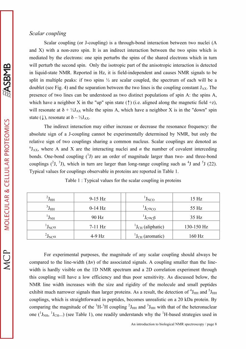
The indirect interaction may either increase or decrease the resonance frequency: the absolute sign of a J-coupling cannot be experimentally determined by NMR, but only the relative sign of two couplings sharing a common nucleus. Scalar couplings are denoted as nJAX, where A and X are the interacting nuclei and n the number of covalent interceding bonds. One-bond coupling (1J) are an order of magnitude larger than two- and three-bond couplings (2J, 3J), which in turn are larger than long-range coupling such as 4J and 5J (22). Typical values for couplings observable in proteins are reported in Table 1.

Table 1 : Typical values for the scalar coupling in proteins

2JHH 9-15 Hz 1JNCO 15 Hz 3JHH 0-14 Hz 1JCαCO 55 Hz 1JNH 90 Hz 1JCαCβ 35 Hz

1JNCα 7-11 Hz 1JCH (aliphatic) 130-150 Hz 2JNCα 4-9 Hz 1JCH (aromatic) 160 Hz

For experimental purposes, the magnitude of any scalar coupling should always be compared to the line-width (Δν) of the associated signals. A coupling smaller than the line-width is hardly visible on the 1D NMR spectrum and a 2D correlation experiment through this coupling will have a low efficiency and thus poor sensitivity. As discussed below, the NMR line width increases with the size and rigidity of the molecule and small peptides exhibit much narrower signals than larger proteins. As a result, the detection of 4JHH and 5JHH couplings, which is straightforward in peptides, becomes unrealistic on a 20 kDa protein. By comparing the magnitude of the 1H-1H coupling 2JHH and 3JHH with that of the heteronuclear one (1JNH, 1JCH...) (see Table 1), one readily understands why the 1H-based strategies used in


!

the 70's for protein resonance assignment have been superseded by the triple-resonance approach (see below) relying on much larger heteronuclear couplings.

As scalar couplings stem from the bond orbitals, they all contain structural information. One-bond couplings show little variation for a type of spin pairs: however, 1JCH

for aliphatic carbons (sp3) are smaller than for aromatic carbons (sp2) and for each hybridisation, a rough correlation with the 13C chemical shift has been reported (23). Bax and coworkers (24) have analyzed the variation of the 1JCαHα in proteins [135 Hz -150 Hz] and reported a empirical correlation with the backbone dihedral angles (φ and ψ) of the residue. With this limited variation of the 1J, heteronuclear corrrelation experiments (such as HSQC or HMQC) could be designed to yield 1H-X cross-peaks of homogeneous amplitude.

Similarly, 2J couplings (2JCαN, 2JHNCα...) show empirical correlations with φ and ψ angle but the difficulty lies in the interpretation of the simultaneous dependences on more than a single torsion angle (25). By far, the most valuable structural information is derived from three-bond mediated vicinal couplings (3J): in the early 60's Martin Karplus (26) established a relationship between the dihedral (torsion) angle (Φ) between protons (H–C–C–H) and vicinal coupling 3J. The general form of the Karplus relationship is:

3J(θ) = A cos2 (Φ) + B cos(Φ) + C [2]

and the coefficients A, B and C are parameterized for each combination of nuclei.

In proteins, the 3JHNHα coupling provides information on the φ backbone angle while the 3JHαHβ does on the side-chain χ1 angle (22). In α-helices (φ = –64º ± 7º), a small 3JHNHα is observed (< 4 Hz) while for β-sheets (φ = –120º ± 10º) larger couplings are present (> 4 Hz). Unfortunately, no 3JHH coupling is linked to the other backbone angle ψ, which can be obtained in a 15N labelled peptide using the much smaller 3JHαN.

The β-methylene moiety found in most amino-acids is a prochiral center, i.e. it could become a chiral center by replacing one of the two protons by another group (a deuterium for instance). As a result, the pro-R and the pro-S protons have different chemical shifts. Their stereospecific assignment is achieved by combining several vicinal coupling constants (3JHαHβ1 , 3JHαHβ2 , 3JNHβ1 , 3JC'Hβ1...) and several distance measurements based on nOe information (see below). Similarly, the two CH3 in Leu and Val isopropyl groups need to be stereospecifically assigned. It has been shown that the availability of stereospectific assignment for these prochiral centers improves the accuracy and the precision of the derived NMR structures (27).

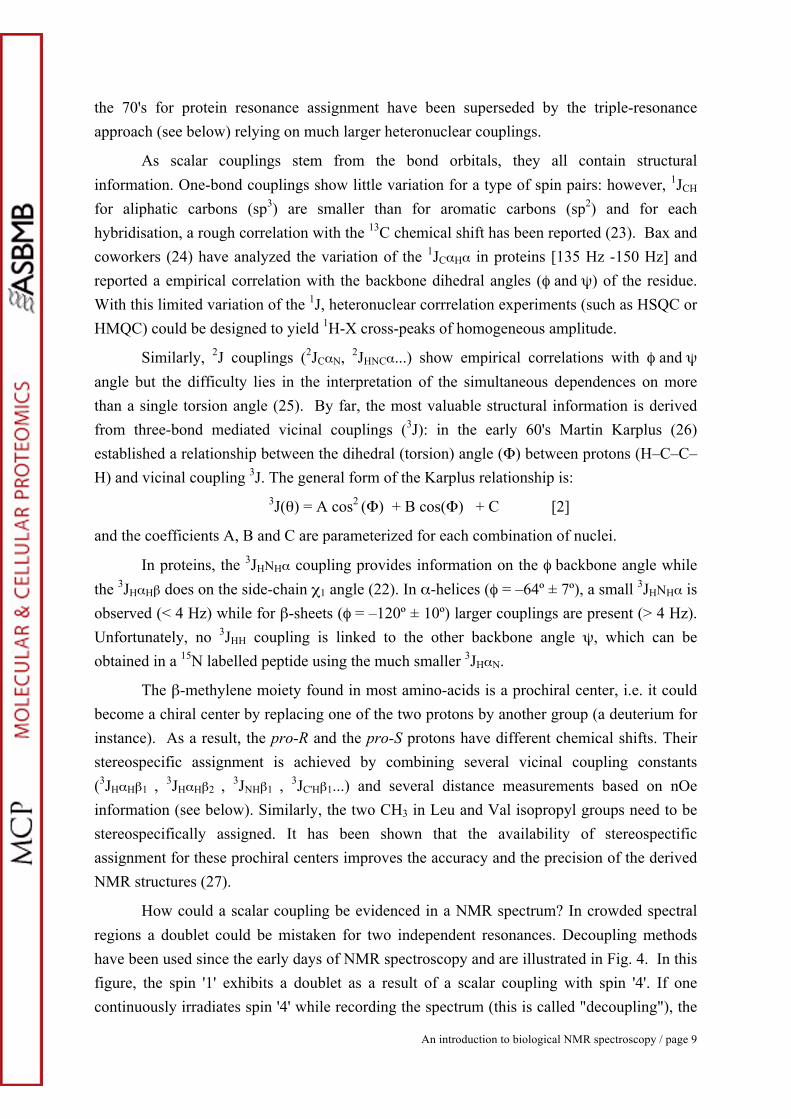
How could a scalar coupling be evidenced in a NMR spectrum? In crowded spectral regions a doublet could be mistaken for two independent resonances. Decoupling methods have been used since the early days of NMR spectroscopy and are illustrated in Fig. 4. In this figure, the spin '1' exhibits a doublet as a result of a scalar coupling with spin '4'. If one continuously irradiates spin '4' while recording the spectrum (this is called "decoupling"), the


!

two lines of '1' will collapse. In presence of decoupling, one can no longer consider two distinct populations of '1' spins (the one next to '1↑' and the other next to '1↓'): their fast interconversion between the two lead to an average resonance frequency for 'a'. Nowadays, these double-irradiation techniques are no longer used and the proof that two spins are scalar coupled can be obtained more conveniently from 2D correlation experiments (COSY or DQF-COSY (28)).

Nuclear Overhauser effect The second kind of anisotropic spin interaction is the dipolar coupling. Though much

larger than the scalar coupling (DNH > 22 kHz), it is not directly visible in liquid-state NMR spectra. All we have to keep in mind at this stage is the fact that the dipolar interaction between A and X depends on the internuclear distance (rAX) and on the orientation of the vector with respect to the magnetic field.

Due to the isotropic tumbling of the molecules in solution, the dipolar coupling averages to zero during the time needed to record the spectrum. It can be detected either in solid-state NMR or when the environment in liquid is no longer isotropic. This later circumstance is encountered when lipid bicelles or bacteriophages are introduced in the sample to induce partial alignment (29) (see section on residual dipolar couplings).

So far we assume that the molecule tumble isotropically in solution. The dipolar interaction acts on the spin system via relaxation mechanisms. Relaxation is the process by which nuclei regain their thermal equilibrium after being perturbed by radiofrequencies. Without relaxation, no NMR experiment could ever be repeated! NMR experiments are carried out in solution where proteins undergo two types of motion as a result of collisions with other proteins and solvent molecules: an erratic random global movement, called Brownian motion, and internal fluctuations at the level of residues, secondary structure elements or domains. All these motions modulate the orientation of the vector with respect to the magnetic field and thus the AX dipolar interaction. This modulation generates radiofrequency (r.f.) fluctuations that contribute to bring the magnetization back to its equilibrium. The spins have been coherently moved away from equilibrium by r.f. pulses and return to this state incoherently by means of motion-induced r.f. fluctuations.

The nuclear Overhauser effect (nOe) (4) was introduced in the historical section as the intensity variation of a metal ion spectrum when their electrons were irradiated. In peptides or proteins, nOe refers to intensity alteration of a spin resonance when other nuclei are irradiated (30). An example is given in Fig. 4: in the lower spectrum, the resonance of spin 'c' is saturated leading to an increase of the amplitude of spin 'a' as compared with the reference spectrum. This effect, also called cross-relaxation, is the evidence of a dipolar interaction between spins 'a' and 'c'. Note that in contrast with the J-decoupling experiment, the


!

multiplicity of 'a' is not altered. As electrons are not mediating the interaction as for J-coupling, nOe is a short range through-space interaction (there is an 1/rAX

6 dependence on distance). This property is pivotal for the application of NMR to structural biology (31): interstrand nOe can be detected in β-sheets, providing not only the nature of the β-sheet (parallel or antiparallel) but also the register of the strands.

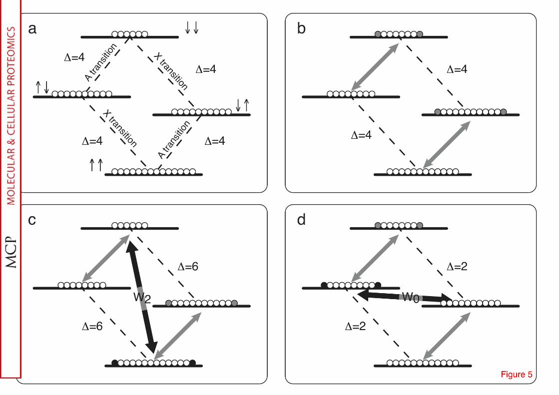
The nOe dependence upon dynamics is depicted in Fig. 5 (see caption for details). In a protein with non uniform flexibility, nOe can only be qualitatively converted into distances. Another annoyance is the phenomenon known as spin diffusion, i.e. the spreading of the nOe along a chain of nuclei. In fact, the magnetization can move to another nucleus by cross-relaxation with a much faster and efficient rate than it decays by auto-relaxation. An analogy in thermodynamics is the heat transfer from an object to a chain of neighbors which occurs much faster than the thermal dissipation. After numerous studies in the 80's to investigate the pitfalls in the conversion of nOe into distances, the following strategies has been established: the identification of a large number of qualitative nOes should be preferred to a small set of accurate distance.

Since the introduction of two-dimensional NMR in the 80's, nOe correlations are no longer obtained by double-irradiation methods (one spin is irradiated and the others are monitored). NOESY experiments (32) provide the same type of information in a more compact manner. It is of interest to notice that the NOESY pulse sequence was designed to investigate any type of exchange process by NMR: a chemical exchange of a species A interconverting into a species B or magnetization transfer between two spins in the same molecule ( A ↔ X ). The two-dimensional approach is handier to use because all neighbors are identified in a single experiment: however, the spin diffusion issue mentioned earlier remains a severe penalty for deriving accurate distances from NOESY spectra (33).

Residual dipolar coupling. In the previous section, we have reported that, in solution, the dipolar coupling is

generally averaged to zero by isotropic motion (see Fig. 6a) and can only be indirectly detected through relaxation effects. In 1995, Tolman et al (34) showed that some small residual dipolar coupling could be observed in cyanometmyoglobin because of the presence of a paramagnetic ion in this protein. The anisotropic magnetic susceptibility of this protein gives rise to a weak alignment and residual dipolar couplings (RDC) were proportional to the square of the static field. Bax and coworkers (35) were able to reproduce similar results on a diamagnetic protein but the observed effects were too weak to have any practical use (1DHN < 0.2Hz).

Various options for increasing the degree of molecular alignment have been searched for. Proteins are generally non-spherically symmetric molecules and when dissolved in a


!

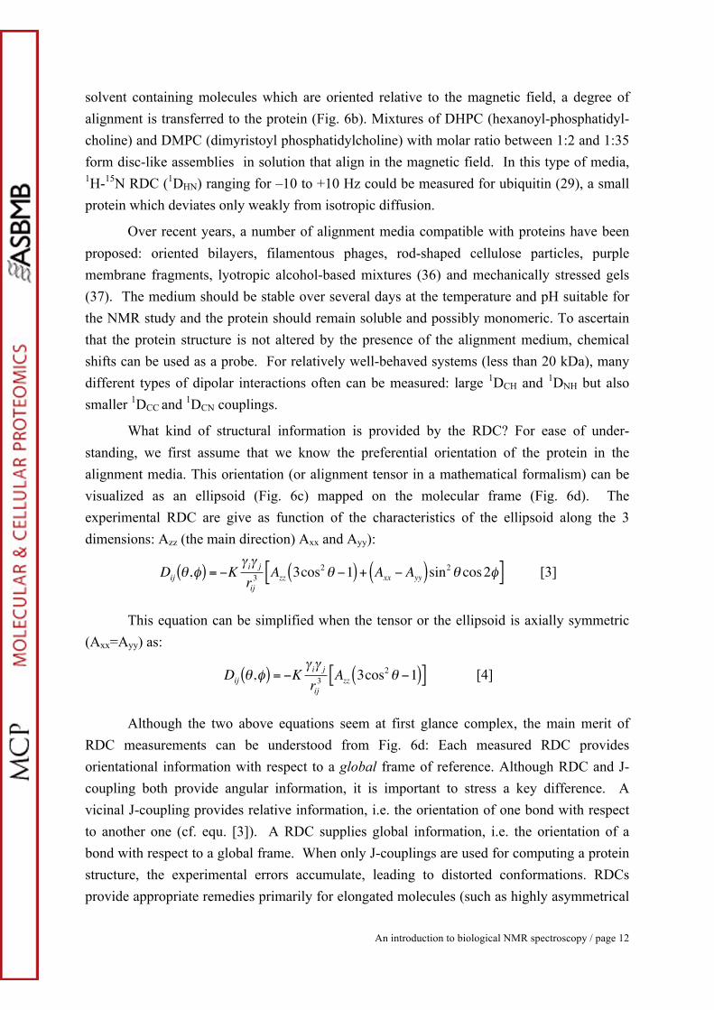
solvent containing molecules which are oriented relative to the magnetic field, a degree of alignment is transferred to the protein (Fig. 6b). Mixtures of DHPC (hexanoyl-phosphatidyl-choline) and DMPC (dimyristoyl phosphatidylcholine) with molar ratio between 1:2 and 1:35 form disc-like assemblies in solution that align in the magnetic field. In this type of media, 1H-15N RDC (1DHN) ranging for –10 to +10 Hz could be measured for ubiquitin (29), a small protein which deviates only weakly from isotropic diffusion.

Over recent years, a number of alignment media compatible with proteins have been proposed: oriented bilayers, filamentous phages, rod-shaped cellulose particles, purple membrane fragments, lyotropic alcohol-based mixtures (36) and mechanically stressed gels (37). The medium should be stable over several days at the temperature and pH suitable for the NMR study and the protein should remain soluble and possibly monomeric. To ascertain that the protein structure is not altered by the presence of the alignment medium, chemical shifts can be used as a probe. For relatively well-behaved systems (less than 20 kDa), many different types of dipolar interactions often can be measured: large 1DCH and 1DNH but also smaller 1DCC and 1DCN couplings.

What kind of structural information is provided by the RDC? For ease of under-standing, we first assume that we know the preferential orientation of the protein in the alignment media. This orientation (or alignment tensor in a mathematical formalism) can be visualized as an ellipsoid (Fig. 6c) mapped on the molecular frame (Fig. 6d). The experimental RDC are give as function of the characteristics of the ellipsoid along the 3 dimensions: Azz (the main direction) Axx and Ayy):

€

Dij θ,φ( ) = −Kγ iγ jrij3 Azz 3cos

2θ −1( ) + Axx − Ayy( )sin2θ cos2φ[ ] [3]

This equation can be simplified when the tensor or the ellipsoid is axially symmetric (Axx=Ayy) as:

€

Dij θ,φ( ) = −Kγ iγ jrij3 Azz 3cos

2θ −1( )[ ] [4]

Although the two above equations seem at first glance complex, the main merit of RDC measurements can be understood from Fig. 6d: Each measured RDC provides orientational information with respect to a global frame of reference. Although RDC and J-coupling both provide angular information, it is important to stress a key difference. A vicinal J-coupling provides relative information, i.e. the orientation of one bond with respect to another one (cf. equ. [3]). A RDC supplies global information, i.e. the orientation of a bond with respect to a global frame. When only J-couplings are used for computing a protein structure, the experimental errors accumulate, leading to distorted conformations. RDCs provide appropriate remedies primarily for elongated molecules (such as highly asymmetrical


!

RNA or DNA) or for multi-domain proteins. RDC provide fast answers to specific structural questions such as conformation changes due to local mutation or ligand binding. Similarly RDC can determine very accurately the relative orientation of domains of known structure or that of interacting partners (38, 39).

Despite the richness of information contained in RDC, several bottlenecks should be mentioned for their measurement and interpretation. Finding suitable alignment media for a given protein may require numerous attempts. Most new media have been first described on test proteins such as ubiquitin, known to be highly well-behaved and stable over long periods of time. The accurate measurement of numerous RDC is a time-consuming task requiring spectrometer time and manual interpretation. The alignment tensor has to be deduced and oriented with respect to the protein using global fitting of all measured RDC in one media: once this orientation is known, a large number of potential solutions for the orientation of each inter-dipolar vector correspond to each measured RDC value. The orientational degeneracy continuum for a single RDC can be lifted by measuring multiple couplings and by using several media leading to differing alignment properties (40).

Two-dimensional NMR and beyond The wealth of information that can be obtained by NMR relies on multi-dimensional

NMR. Any structural investigation starts with the recording of a standard one-dimensional NMR spectrum. This spectrum bears resemblance with spectra obtained with any optical spectroscopy (Infrared, visible, UV): absorption is plotted as function of a frequency or wave-length. For each nucleus, the NMR spectrum displays a signal at a given resonance frequency. We have described earlier that the absolute frequency scale is more conveniently replaced by a scale in ppm to permit comparison between spectra recorded at different fields. In practice, the 1D NMR spectrum is not recorded by sweeping through the entire frequency spectrum: spins are collectively excited by a strong radiofrequency (r.f.) pulse and the resulting signal is then sampled. Its Fourier transform leads to the standard spectrum, i.e. absorption vs frequency. An enormous gain in sensitivity is afforded by this method.

In the early 70's, two-dimensional NMR (9,32) was introduced following a visionary lecture by Jean Jeener: it has been widely used since to correlate the resonance frequencies of several nuclei. In contrast to optical spectroscopy, the information content of a NMR frequency is rather low while a correlation experiment mediated by an interaction (J-coupling or nOe) provides the nature of the partners as well as the interaction strength.


!

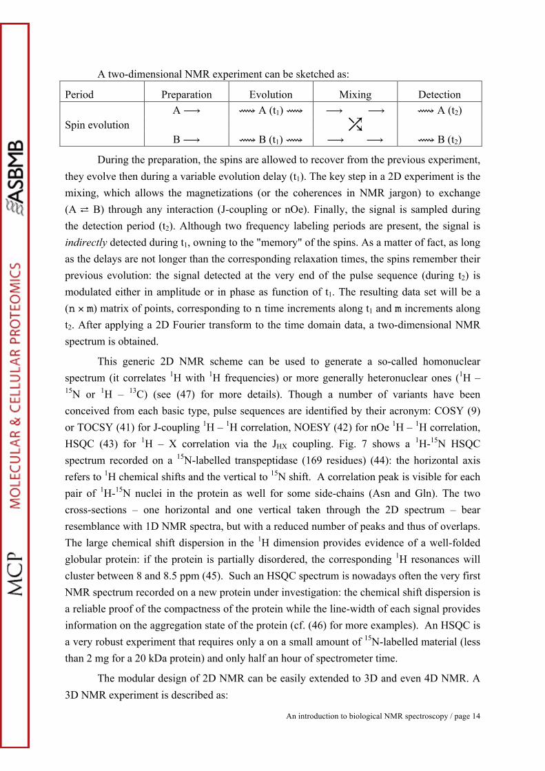
A two-dimensional NMR experiment can be sketched as:

Period Preparation Evolution Mixing Detection A ⟶ ⟿ A (t1) ⟿ ⟶ ⟶ ⟿ A (t2) Spin evolution ⤮ B ⟶ ⟿ B (t1) ⟿ ⟶ ⟶ ⟿ B (t2)

During the preparation, the spins are allowed to recover from the previous experiment, they evolve then during a variable evolution delay (t1). The key step in a 2D experiment is the mixing, which allows the magnetizations (or the coherences in NMR jargon) to exchange (A ⇄ B) through any interaction (J-coupling or nOe). Finally, the signal is sampled during the detection period (t2). Although two frequency labeling periods are present, the signal is indirectly detected during t1, owning to the "memory" of the spins. As a matter of fact, as long as the delays are not longer than the corresponding relaxation times, the spins remember their previous evolution: the signal detected at the very end of the pulse sequence (during t2) is modulated either in amplitude or in phase as function of t1. The resulting data set will be a (n × m) matrix of points, corresponding to n time increments along t1 and m increments along t2. After applying a 2D Fourier transform to the time domain data, a two-dimensional NMR spectrum is obtained.

This generic 2D NMR scheme can be used to generate a so-called homonuclear spectrum (it correlates 1H with 1H frequencies) or more generally heteronuclear ones (1H – 15N or 1H – 13C) (see (47) for more details). Though a number of variants have been conceived from each basic type, pulse sequences are identified by their acronym: COSY (9) or TOCSY (41) for J-coupling 1H – 1H correlation, NOESY (42) for nOe 1H – 1H correlation, HSQC (43) for 1H – X correlation via the JHX coupling. Fig. 7 shows a 1H-15N HSQC spectrum recorded on a 15N-labelled transpeptidase (169 residues) (44): the horizontal axis refers to 1H chemical shifts and the vertical to 15N shift. A correlation peak is visible for each pair of 1H-15N nuclei in the protein as well for some side-chains (Asn and Gln). The two cross-sections – one horizontal and one vertical taken through the 2D spectrum – bear resemblance with 1D NMR spectra, but with a reduced number of peaks and thus of overlaps. The large chemical shift dispersion in the 1H dimension provides evidence of a well-folded globular protein: if the protein is partially disordered, the corresponding 1H resonances will cluster between 8 and 8.5 ppm (45). Such an HSQC spectrum is nowadays often the very first NMR spectrum recorded on a new protein under investigation: the chemical shift dispersion is a reliable proof of the compactness of the protein while the line-width of each signal provides information on the aggregation state of the protein (cf. (46) for more examples). An HSQC is a very robust experiment that requires only a on a small amount of 15N-labelled material (less than 2 mg for a 20 kDa protein) and only half an hour of spectrometer time.

The modular design of 2D NMR can be easily extended to 3D and even 4D NMR. A 3D NMR experiment is described as:


!

Preparation – Evolution (t1) – Mixing#1 – Evolution (t2) – Mixing#2 – Detection (t3)

The resulting spectrum is a three-dimensional spectrum, with 3 frequency axes (F1, F2, and F3), which correlates three different nuclei (11). A 3D pulse sequence can be envisioned as a chemical synthesis with 2 steps (the mixing building blocks): the nature of the reactants, intermediate and final products is identified during the periods t1, t2 and t3 respectively. As for chemical reactions, the overall sensitivity of a 3D NMR relies on the efficiency of the individual transfers and the most sensitive experiments uses exclusively large 1J couplings (cf. Table 1). This observation has led to the design of the triple resonance experiments that will be discussed in the next section.

NMR resonance assignment. NMR resonance assignment is a prerequisite for studies where one aims at deriving

information at the atomic level. Although changes in the spectrum can be monitored even without assignment, the wealth of information is greatly enhanced for assigned signals. Let us consider a titration experiment where an unlabelled protein B is added to a 15N-labelled protein A: if the spectrum of B varies as function of the concentration of A (some signal shifts or get broader), one can already conclude that A and B interact. Note that several biophysical methods (such as fluorescence, fluorescence resonance energy transfer, surface plasmon resonance...) may provide the same information at a much lower cost than NMR.

We mentioned earlier the unique value of NMR, i.e. distinct signals can be resolved even for chemically identical groups which are located in different environments in a protein. Consequently, for well-resolved spectra (narrow lines and optimal digital resolution), one expects to discern one signal for each active spin (1H, 13C or 15N). Before any data can be obtained from spectral parameters, the resonances should be assigned, i.e. a one-to-one correspondence between a nucleus in the molecule and a resonance in the spectrum should be established.

Biologists, who intend to collaborate with an NMR spectroscopist, frequently raise the following question: the structure of a homologous protein has been resolved by X-ray crystallography, does this ease the resonance assignment of my protein? The answer is unfortunately negative. Numerous effects control the NMR chemical shifts and thus, even for a protein with a known structure, it is nearly impossible to predict them. In other terms, the only way to assign resonances is experimental by means of suitable correlation experiments. For lack of being able to directly link a resonance to a nucleus, one will attempt to connect each signal with another, with the ultimate goal of revealing a resonance network with the same topology as the spin network. Accidental resonance overlaps make assignment more challenging: signal discrimination is limited by the spectral resolution (i.e. the linewidth of each signal) and the digital resolution (i.e. the number of experimental points per Hz). The


!

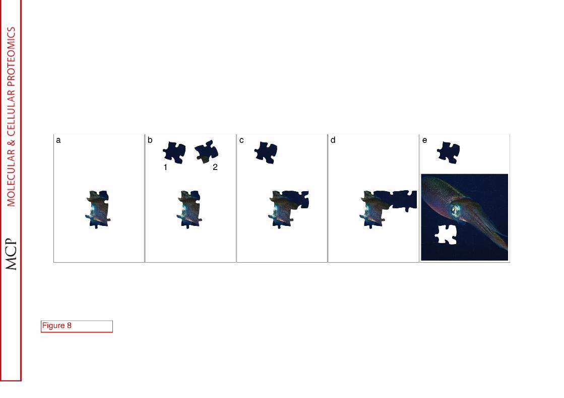
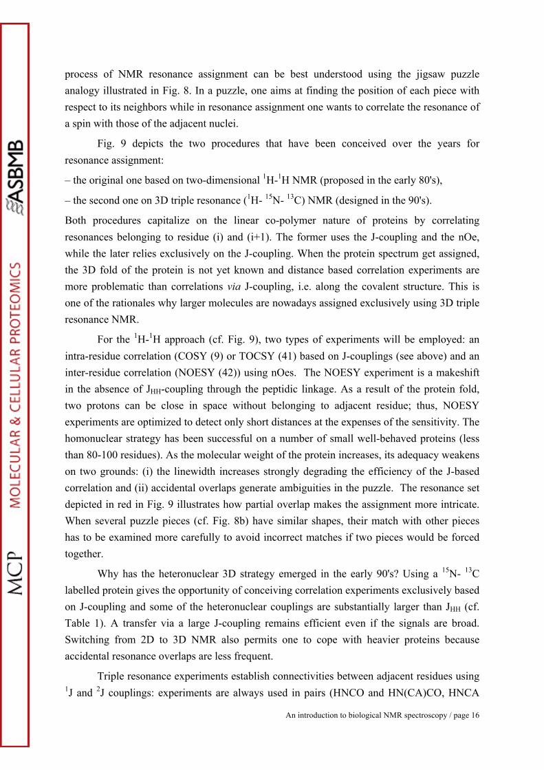
process of NMR resonance assignment can be best understood using the jigsaw puzzle analogy illustrated in Fig. 8. In a puzzle, one aims at finding the position of each piece with respect to its neighbors while in resonance assignment one wants to correlate the resonance of a spin with those of the adjacent nuclei.

Fig. 9 depicts the two procedures that have been conceived over the years for resonance assignment:

– the original one based on two-dimensional 1H-1H NMR (proposed in the early 80's),

– the second one on 3D triple resonance (1H- 15N- 13C) NMR (designed in the 90's).

Both procedures capitalize on the linear co-polymer nature of proteins by correlating resonances belonging to residue (i) and (i+1). The former uses the J-coupling and the nOe, while the later relies exclusively on the J-coupling. When the protein spectrum get assigned, the 3D fold of the protein is not yet known and distance based correlation experiments are more problematic than correlations via J-coupling, i.e. along the covalent structure. This is one of the rationales why larger molecules are nowadays assigned exclusively using 3D triple resonance NMR.

For the 1H-1H approach (cf. Fig. 9), two types of experiments will be employed: an intra-residue correlation (COSY (9) or TOCSY (41) based on J-couplings (see above) and an inter-residue correlation (NOESY (42)) using nOes. The NOESY experiment is a makeshift in the absence of JHH-coupling through the peptidic linkage. As a result of the protein fold, two protons can be close in space without belonging to adjacent residue; thus, NOESY experiments are optimized to detect only short distances at the expenses of the sensitivity. The homonuclear strategy has been successful on a number of small well-behaved proteins (less than 80-100 residues). As the molecular weight of the protein increases, its adequacy weakens on two grounds: (i) the linewidth increases strongly degrading the efficiency of the J-based correlation and (ii) accidental overlaps generate ambiguities in the puzzle. The resonance set depicted in red in Fig. 9 illustrates how partial overlap makes the assignment more intricate. When several puzzle pieces (cf. Fig. 8b) have similar shapes, their match with other pieces has to be examined more carefully to avoid incorrect matches if two pieces would be forced together.

Why has the heteronuclear 3D strategy emerged in the early 90's? Using a 15N- 13C labelled protein gives the opportunity of conceiving correlation experiments exclusively based on J-coupling and some of the heteronuclear couplings are substantially larger than JHH (cf. Table 1). A transfer via a large J-coupling remains efficient even if the signals are broad. Switching from 2D to 3D NMR also permits one to cope with heavier proteins because accidental resonance overlaps are less frequent.

Triple resonance experiments establish connectivities between adjacent residues using 1J and 2J couplings: experiments are always used in pairs (HNCO and HN(CA)CO, HNCA


!

and HN(CO)CA...) to connect residue (i) with residue (i+1). The acronyms used refer to the correlated nuclei and a nucleus denoted with parentheses is used as a relay but not identified (see (47, 48) for a review). Fig. 9 features the combined use of HN(CO)CA and HNCA (49) experiments. In the optimal case, one can thus track the entire polypeptide chain (with the exception of Pro), but supplementary evidence from other experiment pairs is required in practice for heavy peak overlaps. The intrinsic sensitivity of these triple resonance experiments depends upon the nature of the correlated spins (and the coherence pathways between them) and also on the resonance line-width. Thus, it is always difficult to anticipate how laborious a resonance assignment will be: molecular aggregation or internal flexibility will broaden locally the resonances and lead to missing or weak correlation peaks.

With this set of triple resonance experiments (48), the backbone resonance (usually up to the Cβ) can be assigned. Extending the assignment to the entire side-chain is a more tedious and time-consuming task. Do we need to completely assign the side-chains? Yes, if one want to determine the complete 3D structure of the protein. In a number of cases, where the X-ray structure is already available, a NMR study is initiated not to confirm the conformation but to answer questions that could not be addressed by other means. With only the backbone assignment, valuable information can already be obtained: the location of the secondary structure elements (α-helices and β-sheets), the flexibility of the backbone over several time scales (ns, ms...), the affinity and binding site of a ligand. To identify the side-chain resonance, a combination of several 3D experiments are employed, some based on J-coupling transfer (HCCH-TOCSY experiments (50)), some based on nOe effects (13C edited NOESY). Because spectral overlap is more severe than for backbone nuclei, side-chains are generally less completely assigned, an issue that can impact the precision of the derived structures. The stereospecific assignment of the prochiral centers complicates even more the issue: in most amino-acids (with the exception of glycine) the α-carbon is a chiral atom and thus the β-carbon is a prochiral center. As a result of the steric hindrance, the two Hβ exhibit different chemical shifts, as do the two CH3 groups in valine and leucine. Their stereospecific assignment is generally obtained by combining J-coupling values and nOe distances (51), but conformation and dynamics of the side-chains may prevent from gathering this information.

Molecular interactions by NMR

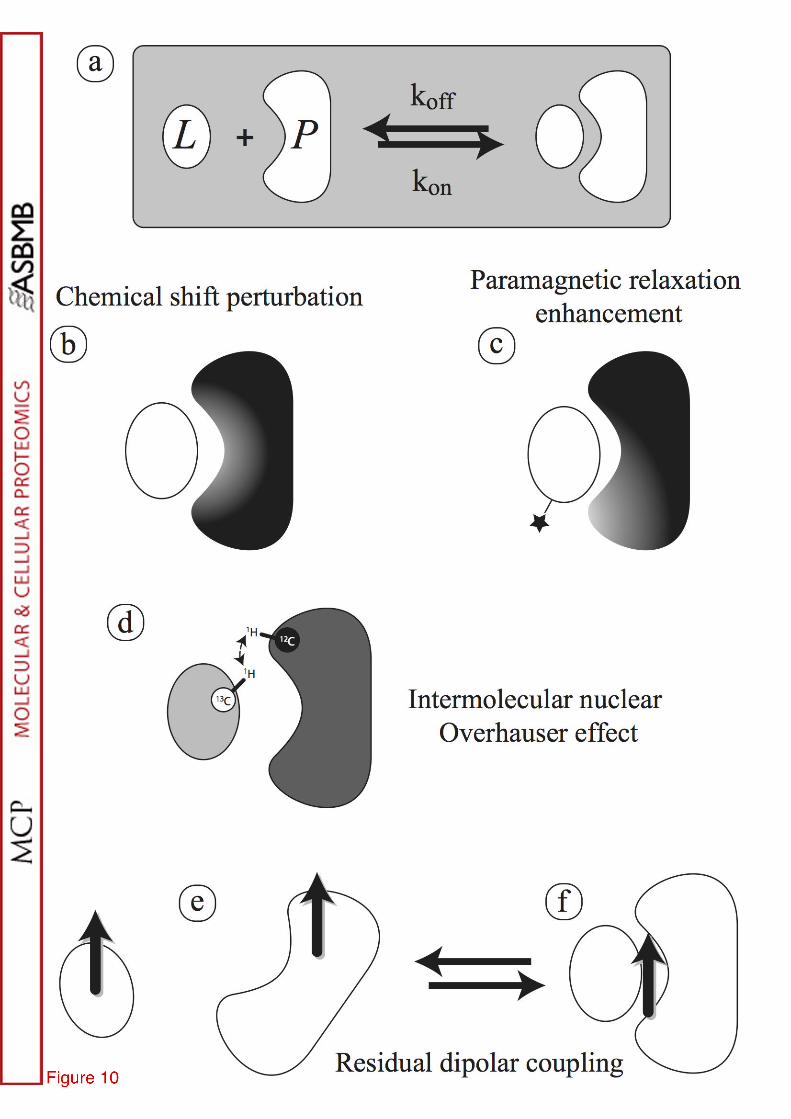
Protein-protein interactions play a key role in numerous cellular processes. Even when two partners have been structurally characterized, co-crystallization of the complex may be difficult due to the low affinity or some local disorder. NMR can complement these studies primarily for weak interactions (Kd > 100 µM). Fig. 10 summarizes various NMR tools for complex studies: chemical shift perturbation, paramagnetic relaxation enhancement, inter-molecular nOe, H/D exchange rates and residual dipolar couplings (52). A prerequisite is the


!

resonance assignment of one of the partners, at least for the backbone. The proteins are expressed and purified separately and, by selective isotopic labeling methods (13C vs 12C or 15N vs 14N), the spectrum of either partner can be hidden.

Widely used, the chemical shift perturbation (CSP) method has been introduced in the early 90's (53, 54) and is based on the observation of the spectrum of one molecule (a 15N-1H HSQC spectrum for instance) with increasing concentration of the partner. When the complex is formed, the two molecules are in equilibrium between their free and bound states. This equilibrium is described by the dissociation constant Kd. During the titration experiment, three exchange regimes can be observed depending on the exchange rate of the complex formation and the chemical shift difference between the free and bound states. In the slow exchange regime, two sets of signals are detected for the two states and their integral can be used to monitor their population. From a practical point of view, this regime is less convenient than the fast one because the complexed signals have to be reassigned de novo. When the exchange between the bound and free forms is fast as compared to the chemical shift differences, the HSQC correlation peaks move in a continuous manner and no new resonance assignment is needed. Analysis of the perturbation reveals which aminoacids are located at the interaction interface (see Fig 10b). Note however that some residues at the far end of the protein may also be slightly perturbed if its global fold is affected. The intermediate regime gives rise to detrimental peak broadening that may prevent the signal observation: one possible work-around is a change in the experimental temperature.

Using CSP, Das et al (55) have studied an antitermination complex involved in prokaryotic transcription regulation: while protein NusB is able to bind individually to a RNA fragment, its affinity is increased by the presence of another factor NusE. The CSP method allowed the authors to investigate not only binary complexes (NusB bound to NusE) but also ternary complexes (NusB / NusE / boxA RNA). Without having to solve the complete 3D structure of this large complex, they were able to identify a loop in NusB that is affected by the other factor NusE in the ternary complex but not in the binary complex. Note that CSP can also be applied to interactions involving intrinsically disordered proteins (56), which are not likely to co-crystallize due to their flexibility.

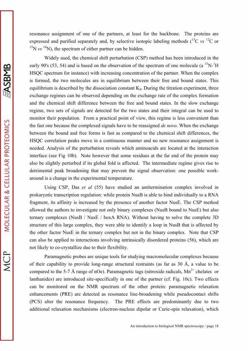
Paramagnetic probes are unique tools for studying macromolecular complexes because of their capability to provide long-range structural restraints (as far as 30 Å, a value to be compared to the 5-7 Å range of nOe). Paramagnetic tags (nitroxide radicals, Mn2+ chelates or lanthanides) are introduced site-specifically in one of the partner (cf. Fig. 10c). Two effects can be monitored on the NMR spectrum of the other protein: paramagnetic relaxation enhancements (PRE) are detected as resonance line-broadening while pseudocontact shifts (PCS) alter the resonance frequency. The PRE effects are predominantly due to two additional relaxation mechanisms (electron-nucleus dipolar or Curie-spin relaxation), which


!

share the same dependence upon the distance from the paramagnetic center (1/r6). The paramagnetic species should be chosen with care to induce moderate broadening without washing out too many signals. Some nuclei such as Gd3+ give large PRE but also no shifts, while others combine the two influences (57). Most lanthanides are introduced using tags covalently bound to a thiol group in the protein, which should engineered by site-directed mutagenesis to contain a single Cys residue. The sketch in Fig. 10c highlights the critical choice the tag position: it should not interfere with the interaction interface but should be close enough to the partner protein.

PRE has been employed to characterize a component of the type III secretion system in Salmonella (58): it contains about 120 copies of a needle protein PrgI (80 residues) and a protein SipD (342 residues) that sits at the tip of the needle. The single native Cys of SipD was mutated to Ser and 14 cysteine mutants were prepared for PRE measurements on the smaller PrgI protein. From this extensive data set, the authors have identified two major sites where PrgI interacts with SipD and correlated these results with invasion assays on mutants.

Short distances are detected by means of nOe inside proteins and this is also applicable to protein complexes. The separate expression and purification of the interaction partner offer the unique opportunity of using isotope labeling to discriminate between intra- and inter-molecular contacts (one protein is 13C-labelled in Fig. 10d). 13C-filtered NMR experiments (59) select spectroscopically intersubunit nOes. Note that for homodimeric structures, this is the only available means to characterize the dimer interface. This approach is best suited for high-affinity complexes (Kd < ~ 50 nM) where the two proteins remain in contact for a longer period of time. For lower affinity, less internuclear nOes can be detected due to line broadening. For example, the recognition of ubiquitin by the third SH3 domain of the yeast Sla1 protein (Kd = ~ 40 nM) has been structurally described by NMR (60): a 15N,13C labelled SH3 domain was titrated with unlabelled ubiquitin and conversely, 15N,13C labelled ubiquitin with unlabelled SH3 domain. While more than 1500 and 1700 intramolecular nOes have been collected for the SH3 domain and ubiquitin in a 1:1 complex, respectively, only 128 intermolecular nOe were identified. The authors have computed NMR-based structure for the complex and concluded that the SH3 domain binds to the canonical binding site for Pro-Rich ligands.

The CSP, PRE and intermolecular nOe data can be used to map the interaction interface and model the complex starting from the known structure of the individual partners obtained independently by X-ray diffraction or NMR. Once the various evidences of the intermolecular interaction have been collected, they can be entered into docking software that will predict the preferred orientation of one molecule to the other. HADDOCK developed by A. Bonvin and colleagues (61) performs data-driven docking using ambiguous interaction restraints (AIR). For any residue in molecule A that exhibits a CSP larger than a given


!

threshold (called an "active" residue), an ambiguous intermolecular distance between this residue and any residue of molecule B is generated. The docking protocol involves a number of optimization steps including the global positioning of the two molecules and the local refinement of the side-chain at the interface. Note that the HADDOCK protocol can use any type of information on the interaction such as site-directed mutagenesis results.

Macromolecular structure by NMR spectroscopy

Over the last decades, NMR has emerged as a technique able to provide structural information on biological molecules and has thus been frequently compared with X-ray crystallography. Let us briefly summarize how a structure is obtained by crystallography: the beam of X-rays strikes the protein crystal producing scattered beams. The measured diffraction pattern is converted into an electron-density map, provided that the phase problem has been solved. The atomic model of the protein is obtained by fitting the protein into this electron-density map. The two bottlenecks of X-ray crystallography are the growth of suitable crystals and the resolution of the phase problem by various means such as molecular replacement or heavy atom methods. The electron-density map is an image of the protein which could be locally blurred as a result of local disorder. In contrast, it is important to remember that the NMR derived 3D representation of the protein is not an image of the real structure (as for X-ray) but a model of that structure that is compatible with the experimental data. In addition, the positional uncertainty in the molecular coordinates is given by the precision and the accuracy of the model, two concepts that are clearly differentiated (62). To clarify these issues, we will start with an overview of the process of protein structure determination by NMR.

With the resonance assignments in hand, one can move to the next step, the structural characterization of the protein. It involves collecting the largest possible number of spectral parameters (primarily nOes, but also J-couplings and residual dipolar couplings): each piece of information entails an amplitude and an assignment. Let us pinpoint this in the case of 1H-1H nOe: each visible cross-peak in a NOESY spectrum leads to an entry containing a peak amplitude and a pair of assigned protons. Conceptually, nOe assignment is different from resonance assignment discussed earlier, though both processes are intertwined. If two nuclei A and B have almost the same chemical shift (νA – νB ≪ δνA or δνB , where δν is the linewidth), this results in an ambiguous nOe assignment: is C close to A or to B? In the absence of additional information, this nOe cannot be unequivocally unravelled. The observed peak may also arise from the sum of two distinct interactions, C–A and C–B. Furthermore, if all resonances have not been assigned, an observed nOe can potentially involve an unassigned partner (D–X) and be inappropriately assigned to another nuclei (D–A). When examining an


!

NMR based-structure, it is important to keep in mind the two bottlenecks: some distance restraints may be either hidden due to overlaps or misinterpreted by the spectroscopist.

In the early days of NMR, the quantification of the nOe cross-peaks and their conversion into distances was extensively debated: could multi-spin effects (or spin-diffusion) strongly corrupt the evaluation of distance restraints (63). It is now recognized that a qualitative assessment of distances is sufficient: strong cross-peaks are interpreted as a short distance (d < 3.5 Å) and weak peaks as longer distance (d < 5-6 Å). In terms of precision and accuracy of resulting structure, it is advisable to invest more effort in a large set of qualitative distances than in a smaller set of precise distances. The occurrence of a nOe cross-peak is interpreted as an upper bound restraint (d < 5-6 Å) but its absence is seldom included as an lower bound restraint (d > 7 Å): a peak might not be visible for many reasons such as overlap or broadening due to conformational flexibility. As a result, only attractive experimental distance restraints that promote a compact folded structure are included.

This complicated and repetitive procedure, which involves a substantial book-keeping effort, has been recently automated. The resonance assignments are used to generate tentative assignments for nOe peaks in a computer program that converts them into distances and generates a first bundle of structures. The software uses this first set to discard tentative assignments that are conflicting with the majority of these structures and to extend the resonance assignment list. A new set of structures is then computed and the cycle is repeated. This strategy is implemented in several packages: ARIA2 (64), CYANA (65), UNIO (ATNOS/CANDID) (66)... The challenge for such software is to be able to cope with three issues: (i) incomplete or incorrect resonance assignment (primarily for side-chains), (ii) incorrect peak-picking and (iii) nOe cross-peaks that cannot be yet assigned unambiguously (67, 68). Automated procedures perform well if the chemical shifts (including side-chains) have been assigned above 90% completeness. Although their reliability in identifying peaks is lower than a spectroscopist who visually inspects the spectra, these algorithms easily compensate by the information redundancy.

To compute a 3D structure from NMR restraints, most software use a similar strategy, namely restrained molecular dynamics (rMD) simulation or simulated annealing. The qualifying term "restrained" indicates that the simplified force field based on the protein covalent structure (van des Waals interaction and peptide plane planarity) is complemented by a pseudo force field combining all NMR-derived conformational restraints. The conformational landscape of a protein contains numerous local minima, in which optimization algorithms could be trapped. Annealing (heating and controlled cooling) is used in metallurgy to relieve internal stresses and defects in metals and optimize their mechanical properties. To overcome energy barriers and converge towards a global minimum, the rMD simulation is first carried out at higher temperature (the atoms have high kinetic energy) and with a


!

simplified force field to speed up the calculation. The process is repeated from several random initial structures to sample more extensively the conformational landscape. There are fundamental differences between standard MD simulations and rMD simulations in the context of NMR: due to the experimental restraints, the trajectory bears no resemblance to a 'real-life' simulation and is only used as a tool to compute a physically meaningful structure that satisfies the experimental data. At the end of the protocol, the molecule is cooled down, a MD simulation with a complete force field (Lennard–Jones and electrostatic interactions) in a box filled with explicit water molecules is performed.

The computed structures can be envisioned as models that represent our experimental data. It is then necessary to define the quality of the proposed structures: as the true structure is not known, evaluating the accuracy is not realizable. How well the models agree with the NMR restraints can be assessed more easily as well as its conformity to standard features (bond length, bond angle). Along with the bundle of structures deposited in the protein data bank (see Fig. 11), the authors will provide NMR and structure statistics (44): the number of distance and dihedral constraints, the violation of these constraints in terms of mean and standard deviation, the deviation from idealized geometry (bond length and angles) and pairwise rmsd for the heavy atoms and the backbone. Recently a suite of programs, CING (69), was presented to validate the structural NMR ensembles at the residue level: it reports potential issues and directs the attention of the spectroscopist to specific residues that deserves extensive manual verification.

The NMR rmsd can be compared with the B-factors reported for X-ray structures, which give an estimate of anisotropic displacement of each atom about its mean position. However, in contrast with B-factors, rmsd are only a measure for the precision of the data. It has been reported (70) that it overestimates the accuracy of the NMR structure ensemble because the structure calculation procedures underestimate the conformation freedom in proteins.

Proteins that contain disordered domain are usually difficult (if not impossible) to crystallize and can thus be good candidates for a NMR study. A number of proteins are made of several independent globular domains connected by flexible linkers. The linker flexibility, essential for the biological function of the protein, may prevent the growth of crystals for X-ray diffraction. This capacity of NMR has been recently illustrated by Gronenborn and coworkers (71) who have reported the solution structure of a lectin in which a LysM domain is inserted between individual repeats of a single CVNH domain. Two flexible linkers of 7 residues connect the domains but no fixed orientation between them is derived from the NMR data (due to lack of any nOe between the linker and either of the domains). In such a case, NMR is able to derive the structure of each of the domains with high precision (rmsd < 0.25


!

Å on the backbone) while it is likely that false interdomain contacts would have been detected by X-ray crystallography (due to crystal packing) if some crystals could have been produced.

Protein dynamics by NMR The biological function of a protein is intricately linked to its structure but also to its

dynamics. Time-dependent fluctuations in the conformation occur during enzymatic activities, protein folding, regulation... NMR is sensitive to fluctuations in many distinct time windows ranging from ps to sec and can generally be complemented (only for fast motions) by in silico protein dynamics simulations. The first repercussion of dynamics on a NMR spectrum is the resonance line-width: a small molecule exhibits narrow lines while large proteins have broad signals. This line-broadening primarily arises from the slow tumbling of large proteins but is mitigated by protein flexibility: fast internal fluctuations (> ns) narrow the signals while slower motions (ms range) act in the opposite direction. Besides the line-width effect, an array of NMR experiments provides more detailed information on both the global and internal dynamic in proteins (72).

Real-time NMR involves recording a series of NMR spectra after initiating the process under investigation (protein folding, amide proton exchange, pH jump, ligand binding...) using a rapid-mixing apparatus. Despite of the low sensitivity of NMR as compared to fluorescence or absorbance, the time resolution can range from 1 to 10 s. Historically limited to 1D NMR, real-time NMR has gained spectral resolution with the introduction of fast-pulsing 2D NMR (73), where the interscan delay is reduced in combination with selective excitation pulses. With these tools, Schanda et al (74) have studied the folding of α-lactalbumin (starting from a molten-globule state) and the amide hydrogen exchange kinetics during ubiquitin unfolding.

Another NMR experiment becomes more adapted for slower processes (10 ms to 5 s): the exchange spectroscopy method or EXSY (32). Although the pulse sequence is identical to NOESY, the spins but not only the magnetizations are transferred in the present case. The process (A ⇄ B) should be in the slow exchange regime, i.e. kex≪| νA–νB |, with two distinct signals visible for A and B. The 2D cross-peak intensities (A→B and B→A) are quantified for different values of the exchange time T, with an upper limit set to the T1 relaxation time of the resonances. For example, the interaction of the SH3 domain (~60 aa) from the Fyn tyrosine kinase with proline-rich peptides was studied using EXSY(75): dissociation rate constants (koff) as well as thermodynamic parameters were derived from the NMR data combined with Isothermal Titration Calorimetry (ITC). If the exchange process is no longer in the slow exchange regime, the two lines start broadening and then merge. Note that the spectral appearance depends upon the kinetic parameters and not directly upon the binding affinity, though tighter binding yields generally longer-lived bound states.


!

The broadening due to µs-ms molecular motion can be exploited in the CPMG relaxation dispersion experiment. By applying a variable number of 180º refocusing pulses, the dephasing due to the A to B magnetization jumps can be suppressed: the transverse relaxation rate R2

obs (which is the inverse of the line-width) decreases with more 180º pulses. For a two-site exchange model (A ⇄ B), the dispersion profiles are governed by the rate of the exchange process, the chemical shift difference and the relative population pA and pB. This experiment remains operative in cases with strongly skewed populations (pA≪ pB), where the minor species is nearly invisible in the NMR spectrum (76). This methodology can detect low-populated excited states associated with local unfolding events in proteins: the chemical shifts of the intermediate state extracted indirectly from CPMG experiments allow its conformation to be characterized. CPMG relaxation has been used to investigate mutated proteins, where the replacement of a single residue slightly destabilizes the global fold (76) or to protein-peptide complexes with a small (~ 10%) mole fraction of bound peptide (77). Excited invisible states are present along the folding/refolding pathways and in conformational changes during catalysis or ligand binding.

The rate at which the magnetizations relax to equilibrium after excitation is governed by the global and internal dynamics of proteins: the overall rotational diffusion occurs in the ns time scale and the internal fluctuations on the ps time scale. Studies of motions of N–H bonds from amide groups provide site-specific probes for all protein residues (except Pro). Two mechanisms contribute to the relaxation in the 15N-1H pair, the 15N chemical shift anisotropy and the 15N-1H dipolar interaction discussed earlier. Three relaxation parameters for the 15N-1H pair (longitudinal relaxation R1, transverse relaxation R2 and {1H}-15N nOe) (78) are combined to obtain the timescale (correlation time, τm) and the amplitude (order parameter, S2) of the internal motion. Such a separation of the internal and global motions is possible only if they are not correlated (79), an assumption supported by their frequency difference. Note that, in contrast to chemical exchange, NMR relaxation cannot see internal fluctuations that are slower than the global rotation of the protein. The backbone dynamics can be complemented by relaxation studies using side-chain probes (2H relaxation in CD3 groups of aliphatic side-chains) (80). When proteins are comprised of multiple domains separated by flexible linkers, their location can be identified by 15N relaxation as shown for HscB, a 20 kDa cochaperone protein involved in the iron-sulfur cluster biogenesis (81): the linker between the two domains is revealed in the NMR study by low {1H}-15N nOes and R2/R1 ratios and in the crystal state by high backbone B-factors.

Modern NMR spectroscopy offers a rich assortment of techniques to study protein dynamics. Some biologists have expressed criticism of NMR-derived protein dynamics because some time scales are either extremely fast or slow as compared to the biological process. One should concede that ps backbone fluctuations are loosely correlated with enzymatic reactions in the ms range and that real-time NMR can mainly visualize artificially


!

slow biological events. With these limits in mind, NMR remains the only experimental technique to report protein dynamics at atomic resolution over such a wide range of time scale.

NMR of intrinsically disordered proteins For many years NMR has followed the footsteps of X-ray crystallography and focused

on globular proteins composed on regular secondary structure elements. The aim of a protein NMR study was the 3D structure determination and disordered regions (linkers, loops or sequence termini) were overlooked. From eukaryotic genome sequencing, it has been established that more than 30% of the proteins are comprised of disordered regions of more that 50 residues, while carrying out important biological functions (82). The amino-acid composition of intrinsically disordered proteins (IDP) is makedly different from globular counterparts with an increased content of Ala, Arg, Gly, Gln, Ser, Glu, and Lys and Pro. Because of their intrinsic disorder, IDPs cannot be crystallized and thus NMR (83) and small-angle X-ray scattering (SAXS) have contributed most to their studies.

The resonance assignment of IDP NMR spectra follows the same rules as for globular proteins but with two major differences acting in opposite directions: IDPs exhibit a comparatively restricted HN chemical shift dispersion but a more favorable line-width because of the flexibility of the polypeptide chain. Triple resonance experiments can thus be tailored for IDPs in two ways: a better digital resolution can be achieved by sampling all directions for longer time (non-uniform sampling (84)) and the resonance can be spread in additional dimensions in experiments with higher dimensionality (85). This strategy has been successfully applied to a challenging molecule, the 441-residue Tau protein: using 5D to 7D correlation experiments, this disordered protein involved in Alzheimer disease has been automatically assigned (85).

Once the resonances have been assigned, it becomes possible to measure NMR parameters, keeping in mind that they are both ensemble- and time-averaged. Chemical shifts, residual dipolar coupling, nOe and PRE provide access to information at atomic resolution. Although thought as globally disordered, IDPs deviate locally and globally from the "random coil" state and exhibit local structural propensity as well as transient long-range contacts. An NMR investigation aims at identifying these deviations from a random state, either for the free protein or upon interaction with other cellular components.

For globular proteins, we have seen that chemical shifts (in particular 13C shifts) report on the local physico-chemical environment: the covalent structure, the type of amino-acid, and finally on the secondary structure elements. These latter elements are typically transient, confined to short fragments (5-10 residues) and sparsely populated. To reliably interpret these small secondary shifts, it is necessary to used improved references for random coil values


!

(nearest neighbor contribution (86)), to look at shifts from several nuclei and to combine them. The local structural propensity could also be characterized using J-couplings or short range nOes, but this approach has not been much pursued owing to the complexity of the averaging processes. In contrast, residual dipolar couplings (RDC) are more promising tools as they sample an angular dependence with respect to a common frame of reference. Let us consider the RDC associated with a 1H-15N pair: due to the orientation of the NH vector, this coupling will change sign in a transient helical element as compared to an unfolded chain (87).

In the absence of preferred long-range interactions as in globular proteins, long-range contacts are inherently transient and multiple. If intramolecular contacts occur, the hydrodynamic radius of the protein as measured by analytical centrifugation or SAXS is expected to decrease. As far as NMR is concerned, nOe are not suited to detect long-range contacts: their range is rather limited (5-7Å) and their build-up is much slower (>50 ms) than the life time of the contacts. In an earlier section, we have seen that the dipolar interaction involving a paramagnetic center has a much longer range (30-35 Å): chelating groups can be introduced at various locations of the sequence and the PRE effect is measured on the protein signals. One first assumes that the polypeptide chain is an idealized random coil and computes the average distance and the PRE broadening expected for each signal. Any deviation from this theoretical profile is evidence of one or several long-range contacts. Sung and Eliezer (88) have compared the PRE profiles for α-synuclein and homologuous β- and γ-synuclein: less extensive transient long-range contacts are observed in the β- and γ-synuclein, that also have been reported to exhibit less aggregation in vitro. Such differences, which may have some implications in Parkinson's disease, can hardly be obtained by any other experimental technique.

Conclusion

NMR is nowadays an established tool in the field of structural biology. Recent developments in isotopic labeling, magnet technology, electronics and spectroscopy have pushed the boundaries of biomolecular NMR. NMR spectral parameters (J-coupling, nOe, RDC and to a lesser extent chemical shift) provide conformational information at the atomic level on proteins. Once the NMR spectra have been assigned, these angular or distance data are primary sources of information for structure computation. Molecular interactions (with a small co-factor, a RNA fragment or another proteins) can be mapped using the same spectral parameters. In recent years, NMR has become a major tool in the field of intrinsically disordered proteins that are unlikely to crystallize. The dynamics of proteins over a wide range of time scale is investigated using real-time NMR, exchange spectroscopy or relaxation measurements. The major limitation of NMR remains the size of the proteins although


!

proteins up to 1 MDa have been partially studied. Slowly, the NMR field is moving from the development stage to the information-gathering stage. Solid-state NMR has not been discussed in this review but is becoming a complementary tool especially for large soluble multimeric proteins or membrane bound macromolecules. Another emerging field of research is in-cell NMR spectroscopy to delineate the role of complex and crowded cellular environments on protein structure and function. In terms of the number of proteins studied, NMR spectroscopy cannot compete with other high-throughput methods in the proteomics area but provides an alternate view on many systems of biological interest.

Acknowledgments: The authors would like to thanks Dr. Adrien Favier and Dr Michael Caffrey (Univ. of

Illinois at Chicago) for critically reading the manuscript, Dr. Catherine Bougault for providing NMR data, Dr. Rainer Kümmerle (Bruker Fällanden-CH) for providing the NMR spectrometer picture.


!

References: !

!!!!!!!!!!!!!!!!!!!!!!!!!!!!!!!!!!!!!!!!!!!!!!!!!!!!!!!!1 Bloch, F., Hansen, W.W. and Packard, M. (1946) The nuclear induction experiment. Phys. Rev. 70, 474–485. 2 Purcell, E.M., Torrey, H.C., and Pound, R.V. (1946) Resonance absorption by nuclear magnetic moments in a solid. Phys. Rev. 69, 37–38 3 Proctor, W.G. and Yu., FC. (1950) The dependence of a nuclear magnetic resonance frequency upon chemical compound. Phys. Rev. 77, 717-717. 4 Overhauser, A.W. (1953) Polarization of nuclei in metals Phys. Rev. 92, 411–415 5 Freeman, R. and Whiffen, D.H. (1961) Determination of the relative signs of proton spin coupling constants by double irradiation Mol. Phys. 4, 321–325. 6 Nelson, F.A and Weaver, H.E. (1964) Nuclear magnetic resonance spectroscopy in super-conducting magnetic fields. Science 146, 223–32. 7 Ernst, R.R and Anderson, W.A. (1966) Application of Fourier transformed spectroscopy to magnetic resonance. Rev. Sci. Instrum. 37, 93–102. 8 Saunders, M., Wishnia, A. and Kirkwood, J.G., (1957) The nuclear magnetic resonance spectrum of ribonuclease, J. Am. Chem. Soc. 79, 3289–3290 9 Aue, W.P., Bartholdi, E., and Ernst, R.R., (1976) Two-dimensional spectroscopy. Application to nuclear magnetic resonance, J. Chem. Phys. 64, 2229–2246 10 Williamson, M.P., Havel, T.F. and Wüthrich, K. (1985) Solution conformation of proteinase inhibitor IIA from bull seminal plasma by 1H nuclear magnetic resonance and distance geometry. J Mol Biol. 182, 295–315. 11 Bax, A. (1994) Multidimensional nuclear magnetic resonance methods for protein studies. Curr Opin Struc Biol 4, 738–44. 12 Mittermaier, A.K. and Kay, L.E. (2009) Observing biological dynamics at atomic resolution using NMR. Trends Biochem Sci 34, 601–11. 13 Pellecchia, M., Bertini, I., Cowburn, D., Dalvit, C., Giralt, E., Jahnke, W., James, T.L., Homans, S.W., Kessler, H., and Luchinat, C. (2008) Perspectives on NMR in drug discovery: a technique comes of age. Nature Reviews Drug Discovery 7, 738–45. 14 Shen, Y., Delaglio, F., Cornilescu, G. and Bax, A., (2009) TALOS+: a hybrid method for predicting protein backbone torsion angles from NMR chemical shifts, J. Biomol. NMR 44, 213–223. 15 Bundi, A. and Wüthrich, K. (1979) 1H-NMR parameters of the common amino acid residues measured in aqueous solutions of the linear tetrapeptides H-Gly-Gly-X-L-Ala-OH," Biopolymers 18, 285–297 16 Wishart, D.S. (2011) Interpreting protein chemical shift data. Prog Nucl Mag Res Sp 58, 62–87. 17 Zhang, H., Neal, S. and Wishart, D.S., (2003) RefDB: a database of uniformly referenced protein chemical shifts, J. Biomol. NMR 25, 173–195. 18 Wishart, D.S., Sykes, B.D., and Richards, F.M. (1992) The chemical shift index: a fast and simple method for the assignment of protein secondary structure through NMR spectroscopy. Biochemistry 31, 1647–1651 19 Wishart, D.S. and Sykes, B.D. (1994) The 13C chemical-shift index: a simple method for the identification of protein secondary structure using 13C chemical-shift data. J. Biomol. NMR 4, 171–80.


!

!!!!!!!!!!!!!!!!!!!!!!!!!!!!!!!!!!!!!!!!!!!!!!!!!!!!!!!!!!!!!!!!!!!!!!!!!!!!!!!!!!!!!!!!!!!!!!!!!!!!!!!!!!!!!!!!!!!!!!!!!!!!!!!!!!!!!!!!!!!!!!!!!!!!!!!!!!!!!!!!!!!!!!!!!!!!!20 Cornilescu, G., Delaglio, F. and Bax, A. (1999) Protein backbone angle restraints from searching a database for chemical shift and sequence homology, J. Biomol. NMR 13, 289–302. 21 Shen, Y., Lange, O., Delaglio, F., Rossi, P., Aramini, J.M., Liu, G., Eletsky, A., Wu, Y., Singarapu, K.K., Lemak, A., Ignatchenko, A., Arrowsmith, C.H., Szyperski, T., Montelione, G.T., Baker, D. and Bax, A. (2008) Consistent blind protein structure generation from NMR chemical shift data. P Natl Acad Sci Usa 105, 4685–90. 22 Bystrov, V.F. (1976) Spin-spin coupling and the conformational states of peptides systems. Prog Nucl Mag Res Sp 10, 41–81. 23 Zwahlen, C., Legault, P., Vincent, S.J.F., Greenblatt, J., Konrat, R. and Kay, L.E. (1997) Methods for measurement of intermolecular NOEs by multinuclear NMR spectroscopy: application to a bacteriophage λ N-peptide/boxB RNA complex. J. Am. Chem. Soc. 119, 6711–21. 24 Vuister, G.W., Delaglio, F. and Bax, A. (1992) An empirical correlation between 1JCαHα and protein backbone conformation. J. Am. Chem. Soc. 114, 9674–9675.! 25 Schmidt, J.M., Hua, Y. and Löhr, F. (2010) Correlation of 2J couplings with protein secondary structure. Proteins 78, 1544–62. 26 Karplus, M. (1963) Vicinal proton coupling in nuclear magnetic resonance. J. Am. Chem. Soc. 85, 2870–2871 27 Güntert, P., Braun, W., Billeter, M. and Wüthrich, K. (1989) Automated stereospecific proton NMR assignments and their impact on the precision of protein structure determinations in solution. J. Am. Chem. Soc. 111, 3997–4004. 28 Piantini, U., Sorensen, O.W. and Ernst, R.R. (1982) Multiple quantum filters for elucida-ting NMR coupling networks. J. Am. Chem. Soc. 104, 6800–6801 29 Tjandra, N. and Bax, A. (1997) Direct measurement of distances and angles in biomolecules by NMR in a dilute liquid crystalline medium. Science 278, 1111–1114 30 Neuhaus, D. and Willamson, M.P. (1989) The nuclear Overhauser effect in structural an conformational analysis. VCH publishers, Inc New York 31 Williamson, M.P. (2009). Applications of the NOE in Molecular Biology. Annu. Rep. NMR Spectrosc. 65, 77–109 32 Jeener, J., Meier, B.H., Bachmann, P. and Ernst, R.R. (1979) Investigation of exchange processes by 2-Dimensional NMR-spectroscopy. J. Chem. Phys. 71, 4546–4553 33 Keepers, J.W. and James, T.L. (1984) A theoretical study of distance determinations from NMR. Two-dimensional nuclear overhauser effect spectra, J. Magn. Reson. 57, 404–426. 34 Tolman, J.R., Flanagan, J.M., Kennedy, M.A. and Prestegard, J.H. (1995) Nuclear magnetic dipole interactions in field-oriented proteins: information for structure determination in solution Proc. Natl. Acad. Sci. U.S.A. 92, 9279–9283 35 Tjandra, N., Grzesiek, S. and Bax, A. (1996) Magnetic field dependence of nitrogen-proton J splittings in 15N-enriched human ubiquitin resulting from relaxation interference and residual dipolar coupling. J. Am. Chem. Soc. 118, 6264–72. 36 Rückert, M. and Otting, G. (2000) Alignment of biological macromolecules in novel nonionic liquid crystalline media for NMR experiments J. Am. Chem. Soc. 122 , 7793–7797. 37 Tycko, R., Blanco, F. and Ishii, Y. (2000) Alignment of biopolymers in strained gels: A new way to create detectable dipole-dipole couplings in high-resolution biomolecular NMR J. Am. Chem. Soc. 122, 9340–9341


!

!!!!!!!!!!!!!!!!!!!!!!!!!!!!!!!!!!!!!!!!!!!!!!!!!!!!!!!!!!!!!!!!!!!!!!!!!!!!!!!!!!!!!!!!!!!!!!!!!!!!!!!!!!!!!!!!!!!!!!!!!!!!!!!!!!!!!!!!!!!!!!!!!!!!!!!!!!!!!!!!!!!!!!!!!!!!!38 Bolon, P.J., Al-Hashimi, H.M. and Prestegard, J.H. (1999) Residual dipolar coupling derived orientational constraints on ligand geometry in a 53 kDa protein-ligand complex. J. Mol. Biol. 293, 107–115 39 Bax, A. and Grishaev, A. (2005) Weak alignment NMR: a hawk-eyed view of biomolecular structure. Curr Opin Struc Biol 15, 563–70. 40 Hus, J.C., Peti, W., Griesinger, C. and Brüschweiler, R. (2003) Self-consistency analysis of dipolar couplings in multiple alignments of Ubiquitin J. Am. Chem. Soc. 125, 5596–5597 41 Davis, D.G. and Bax, A. (1985) Assignment of complex 1H NMR spectra via two-dimensional homonuclear Hartmann-Hahn spectroscopy J. Am. Chem. Soc. 107, 2820–2821 42 Kumar, A., Ernst, R.R. and Wüthrich, K. (1980) A two-dimensional nuclear Overhauser enhancement (2D NOE) experiment for the elucidation of complete proton-proton cross-relaxation networks in biological macromolecules Biochem. Biophys. Res. Commun. 95, 1–6 43 Bodenhausen, G. and Ruben, D.J. (1980) Natural abundance nitrogen-15 NMR by enhanced heteronuclear spectroscopy. Chem Phys Lett 69, 185–189 44 Lecoq, L., Bougault, C., Hugonnet, J.-E., Veckerlé, C., Pessey, O., Arthur, M. and Simorre J.-P. (2012) Dynamics induced by β-lactam antibiotics in the active site of Bacillus subtilis L,D-Transpeptidase. Struct. Fold. Des. 20, 850–61. 45 Marion, D., Tarbouriech, N., Ruigrok, R.W., Burmeister, W.P. and Blanchard, L. (2001) Letter to the Editor: Assignment of the 1H, 15N and 13C resonances of the nucleocapsid-binding domain of the Sendai virus Phosphoprotein. J. Biomol. NMR 21, 75–6. 46 Kwan, A.H., Mobli, M., Gooley, P.R., King, G.F. and Mackay J.P. (2011) Macro-molecular NMR spectroscopy for the non-spectroscopist. FEBS Journal 278, 687–703. 47 Cavanagh, J., Fairbrother, W.J., Palmer, A.G. and Skelton, N.J. (1996) Protein NMR Spectroscopy: Principles and practice; Academic Press: San Diego, CA. 48 Sattler, M., Schleucher, J. and Griesinger, C. (1999) Heteronuclear multidimensional NMR experiments for the structure determination of proteins in solution employing pulsed field gradients Prog Nucl Mag Res Sp 34, 93–158 49 Grzesiek, S. and Bax, A. (1992) Improved 3D triple-resonance NMR techniques applied to a 31 kDa protein. J. Magn. Reson. 96, 432–40. 50 Bax, A., Clore, G.M., Driscoll, P.C., Gronenborn, A.M., Ikura, M. and Kay, LE. (1990) Practical aspects of proton-carbon-carbon-proton 3-dimensional correlation spectroscopy of 13C-labeled proteins J. Magn. Reson. 87, 620–627 51 Constantine, K.L., Friedrichs, M.S. and Mueller, L. (1994) Simple approaches for estimating vicinal 1H-1H coupling-constants and for obtaining stereospecific resonance assignments in leucine side chains. J. Magn. Reson. Ser B 104, 62–8. 52 O'Connell, M.R., Gamsjaeger R. and Mackay J.P. (2009) The structural analysis of protein-protein interactions by NMR spectroscopy. Proteomics 9, 5224–32. 53 Chen, Y., Reizer, J., Saier, M.H., Fairbrother, W.J., and Wright, P.E. 1993. Mapping of the binding interfaces of the proteins of the bacterial phosphotransferase system, HPr and IIAglc. Biochemistry 32: 32–7. 54 Foster, M.P., Wuttke, D.S., Clemens, K. R., Jahnke, W., Radhakrishnan, I., Tennant, L., Reymond, M., Chung, J., and Wright, P.E. (1998) Chemical shift as a probe of molecular interfaces: NMR studies of DNA binding by the three amino-terminal zinc finger domains from transcription factor IIIA. J Biomol NMR 12, 51–71.


!

!!!!!!!!!!!!!!!!!!!!!!!!!!!!!!!!!!!!!!!!!!!!!!!!!!!!!!!!!!!!!!!!!!!!!!!!!!!!!!!!!!!!!!!!!!!!!!!!!!!!!!!!!!!!!!!!!!!!!!!!!!!!!!!!!!!!!!!!!!!!!!!!!!!!!!!!!!!!!!!!!!!!!!!!!!!!!55 Das, R., Loss, S., Li J., Waugh, D.S., Tarasov, S., Wingfield, P.T., Byrd, R.A. and Altieri, A.S. (2008) Structural Biophysics of the NusB:NusE Antitermination Complex. J Mol Biol 376, 705–20. 56 Feuerstein, S., Solyom, Z., Aladag, A., Favier, A., Schwarten, M., Hoffmann, S., Willbold, D. and Brutscher, B. (2012). Transient structure and SH3 interaction sites in an intrinsically disordered fragment of the Hepatitis C virus protein NS5A. J Mol Biol 420, 310–23. 57 Otting, G. (2008) Prospects for lanthanides in structural biology by NMR. J. Biomol. NMR 42, 1–9. 58 Rathinavelan, T., Tang, C. and De Guzman, R.N. (2011) Characterization of the interaction between the Salmonella type III secretion system tip protein SipD and the needle protein PrgI by paramagnetic relaxation enhancement. J. Biol. Chem. 286: 4922–30. 59 Otting, G. and Wüthrich, K. (1990) Heteronuclear filters in 2-dimensional 1H-1H NMR-spectroscopy - combined use with isotope labeling for studies of macromolecular confor-mation and intermolecular interactions. Q Rev Biophys 23, 39–96 60 He, Y., Hicke, L. and Radhakrishnan, I. (2007) Structural Basis for Ubiquitin Recognition by SH3 Domains. J Mol Biol 373, 190–6. 61 Dominguez, C., Boelens, R., and Bonvin, A.M.J.J. (2003) HADDOCK: A Protein−Protein Docking Approach Based on Biochemical or Biophysical Information. J Am Chem Soc 125, 1731–1737 62 Spronk, C.A.E.M., Nabuurs S.B., Krieger, E., Vriend, G. and Vuister, G.W. (2004) Validation of protein structures derived by NMR spectroscopy. Prog Nucl Mag Res Sp 45, 315–37. 63 Clore, G.M. and Gronenborn, A.M. (1985) Assessment of errors involved in the determination of interproton distance ratios and distances by means of one-and two-dimensional nOe measurements. J. Magn. Reson. 61, 158–64. 64 Rieping, W., Habeck, M., Bardiaux, B., Bernard, A., Malliavin, T.E. and Nilges, M. (2007) ARIA2: automated NOE assignment and data integration in NMR structure calculation. Bioinformatics 23, 381–382 65 Güntert, P. (2004) Automated NMR protein structure calculation with CYANA. Meth. Mol. Biol. 278, 353-378. 66 Guerry, P. and Herrmann, T. (2012) Automated protein structure determination methods. NMR of biomolecules: Towards mechanistic systems biology. Bertini I., McGreevy K., Parigi G. (eds.) John Wiley & Sons Ltd., pp 537–548. 67 Linge, J.P., O'Donoghue, S.I. and Nilges, M. (2001) Automated assignment of ambiguous nuclear overhauser effects with ARIA. Meth Enzymol 339, 71–90. 68 Güntert, P. (2008) Automated structure determination from NMR spectra. Eur Biophys J 38, 129–43. 69 Doreleijers, J.F., Sousa da Silva, A.W., Krieger, E., Nabuurs, S.B., Spronk, C.A.E.M., Stevens, T.J., Vranken, W.F., Vriend, G., and Vuister, G.W. (2012) CING: an integrated residue-based structure validation program suite. J Biomol NMR 54, 267–83. 70 Spronk, C.A.E.M., Nabuurs, S.B., Bonvin, A.M.J.J., Krieger, E., Vuister, G.W. and Vriend, G. (2003) The precision of NMR structure ensembles revisited. J. Biomol. NMR 25, 225–34. 71 Koharudin, L.M.I., Viscomi, A.R., Montanini, B., Kershaw, M.J., Talbot, N.J., Ottonello, S. and Gronenborn, A.M. (2011) Structure-function analysis of a CVNH-LysM lectin


!

!!!!!!!!!!!!!!!!!!!!!!!!!!!!!!!!!!!!!!!!!!!!!!!!!!!!!!!!!!!!!!!!!!!!!!!!!!!!!!!!!!!!!!!!!!!!!!!!!!!!!!!!!!!!!!!!!!!!!!!!!!!!!!!!!!!!!!!!!!!!!!!!!!!!!!!!!!!!!!!!!!!!!!!!!!!!!expressed during plant infection by the rice blast fungus Magnaporthe oryzae. Struct. Fold. Des. 19, 662–74. 72 Kleckner, I.R. and Foster, M.P. (2011) An introduction to NMR-based approaches for measuring protein dynamics. BBA - Proteins and Proteomics 1814, 942–68. 73 Schanda, P. and Brutscher, B. (2005) Very fast two-dimensional NMR spectroscopy for real-time investigation of dynamic events in proteins on the time scale of seconds. J. Am. Chem. Soc. 127, 8014–5. 74 Schanda, P., Forge, V. and Brutscher, B. (2007) Protein folding and unfolding studied at atomic resolution by fast two-dimensional NMR spectroscopy. Proc. Natl. Acad. Sci. U.S.A. 104, 11257–62. 75 Demers, J.-P. and Mittermaier, A.K. (2009) Binding Mechanism of an SH3 Domain Studied by NMR and ITC. J. Am. Chem. Soc. 131, 4355–67. 76 Skrynnikov, N.R., Dahlquist, F.W. and Kay, L.E. (2002) Reconstructing NMR spectra of “invisible” excited protein states using HSQC and HMQC experiments. J. Am. Chem. Soc. 124, 12352–60. 77 Hansen, D.F., Vallurupalli, P., Lundström, P., Neudecker, P. and Kay, L.E. (2008) probing chemical shifts of invisible states of proteins with relaxation dispersion NMR spectroscopy: How well can we do? J. Am. Chem. Soc. 130, 2667–75. 78 Kay, L.E., Torchia, D.A. and Bax, A. (1989) Backbone dynamics of proteins as studied by 15N inverse detected heteronuclear NMR spectroscopy: application to staphylococcal nuclease. Biochemistry. 28, 8972–8979. 79 Lipari, G. and Szabo, A. (1982) Model-free approach to the interpretation of nuclear magnetic relaxation in macromolecules: 1. Theory and range of validity. J. Am. Chem. Soc. 104, 4546–4559 80 Choy, W.Y., Shortle, D., and Kay, L.E. (2003) Side chain dynamics in unfolded protein states: an NMR based 2H spin relaxation study of D131D. J. Am. Chem. Soc. 125, 1748–1758. 81 Füzéry, A.K., Tonelli, M., Ta, D.T., Cornilescu, G., Vickery, L.E., and Markley, J.L. (2008) Solution structure of the iron−sulfur cluster cochaperone HscB and its binding surface for the iron−sulfur assembly scaffold protein IscU. Biochemistry 47, 9394–404. 82 Dunker, A.K., Silman, I., Uversky, V.N. and Sussman, J.L. (2008) Function and structure of inherently disordered proteins. Curr. Opin. Struct. Biol. 18, 756–764 83 Dyson, H.J. and Wright, P.E. (2004) Unfolded proteins and protein folding studied by NMR. Chem. Rev. 104, 3607–3622 84 Pannetier, N., Houben, K., Blanchard, L. and Marion, D. (2007) Optimized 3D-NMR sam-pling for resonance assignment of partially unfolded proteins. J. Magn. Reson. 186, 142–9. 85 Narayanan, R.L., Dürr, U.H.N., Bibow, S., Biernat, J., Mandelkow, E., and Zweckstetter, M. (2010) Automatic assignment of the intrinsically disordered protein Tau with 441-residues. J. Am. Chem. Soc. 132, 11906–7. 86 Tamiola, K., Acar, B. and Mulder, F.A.A. (2010) Sequence-specific random coil chemical shifts of intrinsically disordered proteins. J. Am. Chem. Soc. 132, 18000–3. 87 Schneider, R., Huang, J.-R., Yao, M., Communie, G., Mollica, L., Salmon, L., Jensen, M.R., and Blackledge, M. (2011) Towards a robust description of intrinsic protein disorder using nuclear magnetic resonance spectroscopy. Mol. BioSyst. 8, 58. 88 Sung, Y.-H. and Eliezer, D. (2007) Residual structure, backbone dynamics, and inter-actions within the Synuclein Family. J Mol Biol 372, 689–707.


!

Figure captions

Figure 1: Picture of a mid-range NMR spectrometer (Courtesy of Bruker-Fällanden). It is composed of a cryomagnet (center), an electronic console (right) and the user console (left). The strength of the magnet is graded according to the frequency of the 1H NMR signals (here 1H=600 MHz or B0=14T). The magnet dewar contains the superconducting coil (not visible) at liquid helium temperature and a detection probe, which is also cooled at 15–20K to minimize the thermal noise (cryoprobe). The sample is inserted from the top of the bore by means of a pneumatic lift. The r.f. pulse and pulsed field gradients enter the probe from the bottom of the magnet bore and two insulated pipes provide the cooling for the cryoprobe and the temperature regulation of the sample (–20 to 80ºC). Most recent magnets are actively shielded, i.e. the stray field outside the magnet itself is minimized. The electronic console contains a pulse programmer that generates and amplifies r.f. and pulse field gradient pulses sent to the probe and trigger the data acquisition: modern spectrometer are equipped with 4 channels (usually 1H, 13C, 15N and 2H for the frequency-field lock) with independent frequency synthesis and amplification. Although the list price of NMR spectrometers has considerably dropped over the years, it does not depend linearly with the magnetic field. The price ratio for 600, 800 and 950 MHz is roughly 1: 2: 6.

Figure 2: Number of structures deposited to the RCSB protein data bank (http://www.rcsb.org/pdb/) over the years. The number of structures solved by X-ray crystallography is steadily increasing while the NMR-based ones have hit a plateau. In the inset, the data for the early years of crystallography are displayed with an extended vertical scale for clarity. For the former method, the crystallization step remains a major bottleneck but once suitable diffraction data are available, the structure can be obtained rather quickly. NMR is primarily hampered by the limitation in protein size that can be studied: despite that resonance assignment and nOe interpretation have been automated, it still requires more human input during these processes.

Figure 3: Without chemical shifts, NMR structural parameters could not be measured and interpreted at atomic level resolution. In fact, the magnetic field at the nucleus is generally different from the applied field B0: this additional contribution (or screening) arises from the interaction of the surrounding electrons with the applied field. The electron density around each nucleus varies according to its chemical properties (nature, bonds...): in a protein, the amide protons resonate between 6 and 9 ppm while the CH3 groups of aliphatic residues are between 0 and 2 ppm. In aromatic moieties (as found in Tyr, Phe, His and Trp), a ring current is induced by the delocalized π-electrons: this current generates a small magnetic field that adds to the applied field B0. A proton located in the plane of the aromatic ring (Ha) experiences a stronger field while another facing the ring (Hb) perceives a weaker field. Ha is


!

said to be downfield shifted while Hb is upfield shifted. These expressions date back to the early days of continuous wave NMR spectroscopy where spectrometers were operating at constant frequency: to observe proton Ha at a constant frequency, a weaker applied B0 was necessary.

Figure 4: Detection of J-coupling and nuclear Overhauser effects in 1D NMR spectra. The reference spectrum (inset a) contains 4 signals labelled '1' to '4' in this spectra region. Two signals ('2' and '3') are singlets and two are multiplets ('1' and '4'). This multiplicity indicates the number of J-coupled neighbors but not their assignment. In inset b, the signal of '4' has been continuously irradiated during the recording of the spectrum (J-decoupling). The '4' signal is completely bleached out and the two lines of the '1' signal collapse: '1' has been decoupled from '4'. This experiment indicates that spin '1' and '4' are J-coupled, i.e. covalent neighbors in the molecule. In inset c, the signal of '3' has been saturated before the recording of the spectrum (1D nOe experiment). '3' disappears and the intensity of '1' is altered while the fine structure remains unchanged. This experiment evidences a dipolar interaction or a nuclear Overhauser effect between 'c' and 'a': these two nuclei are spatial neighbors (< 5-7 Å): the absence of J-coupling between them indicates that they are separated by more than 5 chemical bonds. The same effect could be detected if spins '1' and '3' would belong to two different but interacting molecules.

Figure 5: Nuclear Overhauser effect in a homonuclear (1H) two-spin system (A and X). The four energy levels (↑↑ , ↑↓ , ↓↑, ↓↓ ) are populated according to a Boltzman distribution (inset a). In the unperturbed case, the population difference is the same for all transitions (Δ = 4). If the A-spin transitions are saturated, the associated populations are equalized (inset b). Then the cross-relaxation mechanisms will attempt to reequilibrate the populations towards the equilibrium shown in inset a. The way this reequilibration will occur, depends on the frequencies generated by the molecular fluctuations: If they are fast (as in a small peptide), the double-quantum transition W2 (between ↑↑ and ↓↓ ) at ωA+ωX will be most efficient (inset c). In contrast, a large protein will emit mainly low frequency fluctuations, which correspond to the zero-quantum transition W0 (↓↑ to ↑↓ ) at ωA–ωX (inset d). The outcome of the reequilibration process will thus be opposite: an intensity increase of the X-spin transition (Δ = 6, positive nOe) is observed for small molecules and a decrease (Δ = 2, negative nOe) for the larger proteins.

Figure 6: In an isotropic medium (such as an aqueous buffer), a diamagnetic protein tumbles nearly isotropically, i.e. all orientations have the same probability (inset a). As a result, the dipolar interaction between two spins goes to zero and is only visible through relaxation parameters. When a weak alignment medium is introduced (inset b), the protein acquires a small preferential orientation: the incomplete averaging of the dipolar interaction leads to residual dipolar couplings (RDC). Between the protein and the alignment medium,


!

the interaction is generally steric but in non-neutral media, long-range electrostatic interactions are dominant. The preferential orientational averaging of the molecule can be described by an alignment tensor with eigenvalues Axx, Ayy and Azz (inset c) in the molecular frame. The measured RDC between two spins depends upon the orientation of the internuclear vector with respect to the alignment tensor (inset d) described by the polar coordinates (φ and θ). Note that several degenerate orientations are compatible with data recorded in a single alignment medium, a degeneracy that can be lifted using media with different steric and electrostatic properties.

Figure 7: 1H-15N heteronuclear single quantum correlation spectrum (HSQC) of B. subtilis L,D-transpeptidase LdtBs (169 residues, concentration 0.7 mM, pH 6.5) recorded at 600 MHz (44). The horizontal axis corresponds to the 1H frequency and the vertical one to the 15N frequency. A correlation peak is observed for each backbone 1H-15N pair (all residues except the N-terminus and Pro) as well as for the side-chain NH2 in Asn and Gln residues. For the side-chains (see 15N = [110, 114 ppm], 1H = [6.5, 8.0 ppm]) two cross-peaks at the same 15N frequency are detected as the two 1Hs are not magnetically equivalent. Two 1D slices taken at the position of the dotted arrows are shown: in the vertical slice are visible all amide 15N which bear a 1H at 7.5 ppm. This illustrates how the introduction of an additional dimension (15N) resolves spectral overlaps in the other one (1H). Note that side-chain 15N resonances can also be observed for Arg, His and Trp.

Figure 8: The jigsaw puzzle analogy for NMR resonance assignment. Within such a puzzle, the global placement of any individual piece cannot be inferred just by its shape and the picture depicted on it. However, its position relative to other pieces can be determined by evaluating the match of the edge profile and the picture. As several candidates can be a priori considered, they are ranked according to a penalty function that accounts for the complementary match of protuberances and pictures. The manufacturing of the pieces is imperfect, leading to some looseness and thus a threshold is defined for the penalty function. In panel (a), two pieces have been already successfully matched. Two possible candidates as neighbors on the right hand side are shown in panel (b): although their shape on the left hand side fits roughly the profile of the already matched pair, only one of the two could be anchored effortlessly in panel (c). This conservative strategy is essential to complete the puzzle because any piece that is forced at an incorrect place will be missing somewhere else. The choice made in panel (c) is confirmed in panel (d) as the edge of the puzzle is reached. Once the complete puzzle is solved (panel (e)), it becomes evident that the piece that was not chosen in panel (c) fits somewhere else. The time required to complete a jigsaw puzzle depends upon 3 factors: the number of pieces, their dissimilitude and the looseness of the match. Similarly, an NMR assignment will be more difficult for a larger protein with moderate chemical shift dispersion if the spectra exhibit poor spectral and digital resolution.


!

Fig. 9: Strategies for sequential resonance assignment in proteins. As proteins are linear co-polymers, these strategies aim at correlating the resonance frequencies of one residue with those of the following one. 2D-1H-1H correlation experiments can be employed on unlabelled proteins and 3D triple resonance experiments are better suited for 15N-13C uniformly labelled molecules. The first approach utilizes two correlations experiments: one using 1H-1H J-couplings (COSY or TOCSY) and one using 1H-1H nOe (NOESY). One has to resort to nOe to link two adjacent residues as no 3JHH coupling is available for this purpose: note that nOe is a through-space effect and that nuclei close in space but not belonging to an adjacent residue may lead to fallacious correlations. This issue is resolved in the 3D triple resonance strategy, which relies exclusively on J-couplings. Triple resonance experiments always works in pairs as illustrated here: HN(CO)CA that correlates the HN and the N of residue (i+1) with the Cα of residue (i) and HNCA that correlates the HN and the N of residue (i+1) with both the Cα of residue (i) and that of residue (i+1). In the HN(CO)CA, the carbonyl 13C act as a relay but its frequency is not detected. The experimental combination links each (HN, N) pairs with the preceding and following Cα's and reciprocally each Cα's with the adjacent (HN, N) pairs.

Fig. 10: NMR detection of molecular interactions. A protein (P) is interacting with a ligand (L) (another protein, a small molecule, a RNA fragment...) with an association constant Ka (inset a). This thermodynamic constant is related to two kinetic constants, the on-rate constant kon and the off-rate constant koff. Ka = kon/koff = [PL] / [P].[L]. The affinity between the two molecules and structural information on the complex can be obtained using several NMR parameters. An unlabelled binding partner is added to a 15N labelled protein: this causes changes in the environment of the protein and therefore the chemical shifts of nuclei at the binding interface (inset b). A paramagnetic tag is added to the ligand (inset c): resonances in the protein that are close to the tag are broadened (or even disappear) while others remains unaffected. Paramagnetic relaxation enhancement (PRE) provides structural restraints up to 30 Å. Short internuclear distances can be detected between nuclei belonging to both partners using intermolecular nOes (inset d): discrimination between intra- and intermolecular nOe can be simplified by specific isotope labeling of a single partner. Residual dipolar couplings provide information of the orientation of internuclear vector with respect to the molecular frame of alignement. If the protein and its ligand align in a different manner when free or bound (inset e), RDCs provide powerful long-range restraints for their relative orientation in the complex when bound.

Fig. 11: NMR-based structure of B. subtilis L,D-transpeptidase LdtBs (169 residues) (44). The antibiotic resistance found in some bacterial strains for some β-lactam antibiotics has been assigned to the presence of this transpeptidase able to form unusual peptidoglycan crosslinks. The 1H-15N HSQC spectrum of this protein is shown in Fig. 7. 20 structures have been computed using 3191 nOe restraints, 286 dihedral restraints (J-coupling) and 169


!

residual dipolar couplings. The pairwise RMSD is 0.70 Å for all heavy atoms and 0.39 Å for the backbone. In the upper part of the figure, the best fit superposition of the backbone of the 20 conformers is shown: some parts of the protein have been precisely characterized (α-helices and β-sheets) while others are less well defined (loops and N- and C-termini). The disorder observed for some residues is very likely due to local flexibility. However, it may also be an experimental artefact due to the fortuitous lack of restraints in this area (incompletely assigned residues, resonance overlaps, few neighbors within a 5 Å range...). To confirm the local flexibility, NMR relaxation measurements can be carried out, keeping in mind that they are only sensitive to specific time scale motions. In the lower part of the figure, another depiction of the transpeptidase as a ribbon representation shows the overall organisation of the molecule from the same point of view.

Dominique Marion

Dominique Marion

Dominique Marion

Dominique Marion

Figure 1

Dominique Marion

Dominique Marion

Dominique Marion

Dominique Marion

Figure 2

Dominique Marion

Dominique Marion

Figure 3

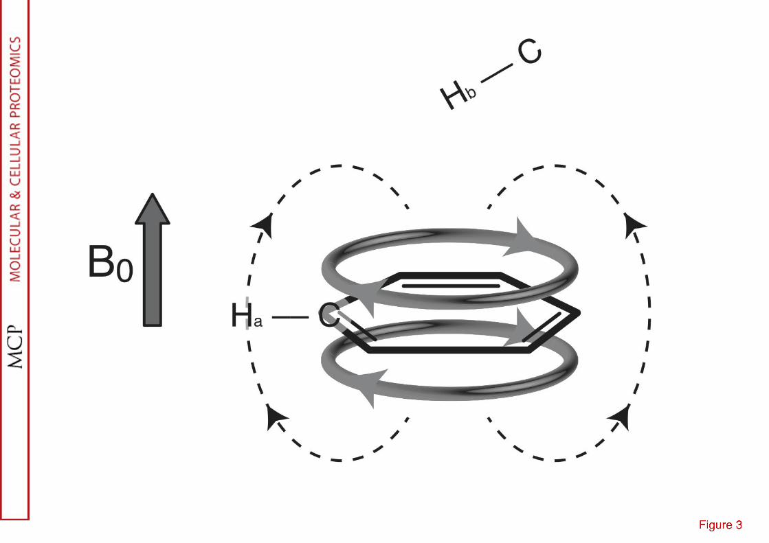
a

b

c

Reference

J-decoupling

Nuclear Overhauser effect

Am

plitu

de

Frequency

Am

plitu

deA

mpl

itude

on qp

Dominique Marion

Figure 4

Dominique Marion

Dominique Marion

Dominique Marion

Dominique Marion

Figure 5

Dominique Marion

Dominique Marion

Figure 6

Dominique Marion

Dominique Marion

Figure 7

Dominique

Figure 8

Dominique Marion

Figure 9

Dominique Marion

Figure 10

Dominique Marion

Figure 11

an introduction to biological nmr spectroscopy# dominique marion

Documents